


1 Introduction
Reactive flow and transport processes in porous media have a wide range of applications such as oil recovery, groundwater remediation and in biomedical contexts. Recently, the investigation of such processes in altering porous structures found an increased interest.
However, due to the physical complexity of the situation, it is not surprising that many analytical results are restricted to very specific situations, e.g. in which no degeneration occurs (up to clogging): In [Reference Agosti, Formaggia and Scotti1] the numerical analysis of a reactive flow problem with non-degenerating, but space-dependent permeability and net dissolution reactions is conducted. In [Reference Dawson and Aizinger9], an advection–diffusion equation with strictly positive porosity, but positive semi-definite diffusion tensor is analysed. In [Reference van Noorden and Muntean29], the existence of global weak solutions of transport and flow in a porous medium with circular inclusions of low permeability is proven. Hereby the porosity, the diffusion and flow profile are prescribed as time-independent non-degenerating $L^\infty$
-functions.In [Reference Gahn, Neuss-Radu and Pop12, Reference Peter20], two-scale convergence of a transport problem and consequently the existence of solutions to the limit problem is proven mapping the evolving geometry to a reference configuration.
$L^\infty$
-functions.In [Reference Gahn, Neuss-Radu and Pop12, Reference Peter20], two-scale convergence of a transport problem and consequently the existence of solutions to the limit problem is proven mapping the evolving geometry to a reference configuration.
The structural alteration and finally clogging of the pore space, which is relevant in many porous media applications, can, however, lead to the degeneration of macroscale parameters namely porosity, permeability and effective diffusion tensor. This poses additional requirements to a thorough analytical treatment: In [Reference Arbogast and Taicher3] two-phase mixtures, e.g. partially melted materials, are considered. The corresponding linear elliptic equations describing the flow at the Darcy scale are derived from mantle dynamics and contain a stabilising pressure term. The key idea in this research to manage the degeneracies arising is to consider an appropriate scaling of the unknowns, more precisely to perform a porosity-weighted transformation of the variables or equivalently to deal with porosity-weighted function spaces. The existence and uniqueness of a solution to the flow problem over the entire domain are then shown using the respective stabilised variational formulation.
Likewise in [Reference Schulz25], the porous medium’s porosity was assumed to be a given time-dependent function, where the degenerate case was of particular interest and thus explicitly admissible. The degeneracy was handled and analytical results were obtained by introducing appropriate weighted function spaces and including the degenerate parameters as weights. In more detail, the non-vanishing parts of the coefficients were proposed that belong to the Muckenhoupt class $A_2$
. Recently, the analysis of degenerating equations of an effective, nonlinear diffusion–precipitation model due to vanishing unknown porosity was conducted in [Reference Schulz26]. There the underlying system was coupled to an evolution equation for the change of porosity. Similar scaling arguments have also been applied to fractured porous media in the case of closing fractures [Reference Boon, Nordbotten and Yotov6], where the vanishing scaling parameter represented the square root of the cross-sectional length of lower-dimensional subdomains.
$A_2$
. Recently, the analysis of degenerating equations of an effective, nonlinear diffusion–precipitation model due to vanishing unknown porosity was conducted in [Reference Schulz26]. There the underlying system was coupled to an evolution equation for the change of porosity. Similar scaling arguments have also been applied to fractured porous media in the case of closing fractures [Reference Boon, Nordbotten and Yotov6], where the vanishing scaling parameter represented the square root of the cross-sectional length of lower-dimensional subdomains.
In this research, we build upon the cited literature, in particular [Reference Arbogast and Taicher3] and extend the results obtained therein. More precisely, we investigate a combined flow and transport model with degenerating porosity, permeability and diffusion. As in [Reference Arbogast and Taicher3, Reference Schulz25], we assume that the change of porosity is prescribed, i.e. there is no evolution equation for the porosity included into the model. Additionally, reasonable linear/power law relations between porosity and diffusion/permeability are used. Finally, we include stabilising terms as used in [Reference Arbogast and Taicher3] for the flow equations, but now also for the transport equations to keep the model consistent. Since the flow and transport model are only one-sided coupled, i.e. there is no back-coupling from the transport to the flow problem, the results from [Reference Arbogast and Taicher3] can be used directly. However, an improved regularity result must be proven for the velocity field to further analyse the transport model. For its analysis, first suitable (uniform) energy estimates equipped with appropriate weights are proven for a regularisation of the degenerating model. With these weighted estimates, we can ultimately pass to the limit and conclude on the existence of weak solutions of the limit problem. The main result is stated in Theorem 3.7.
Finally, we remark that in contrast to our research the investigation of degenerate parabolic equations is usually based on vanishing second ordered terms due to the unknown, cf. [Reference DiBenedetto10]. In porous media applications, such degenerating problems were addressed using Kirchhoff’s transformation, among others, in the context of Richards’ equation [Reference Alt and Luckhaus2, Reference Pop and Schweizer21, Reference Radu, Pop and Knabner23]. Beside the terms of second order, there the time derivative also approaches to 0. For numerical analysis of degenerate reactive transport in the unsaturated regime, we likewise refer to [Reference Eymard, Hilhorst and Vohralk11, Reference Radu, Pop and Attinger22]. However, transport equations can also degenerate due to vanishing porosity which is caused by clogging pores. Although the time derivative and the second-ordered terms are again involved, the mathematical structure is different and thus these degeneracies have up to now barely been analysed.
Outline: In Section 2, we introduce the model under consideration based on the model stated in [Reference Arbogast and Taicher3]. Thereafter, in Section 3, we perform the analysis of the model. More precisely, we recall the analysis of the degenerating flow model from [Reference Arbogast and Taicher3] and discuss the regularity of the velocity field in Section 3.1. Building upon these results as well as on a regularisation of the degenerating transport model, we prove the unique, weak solvability of the degenerating transport model in Section 3.2. Finally, we end with concluding remarks in Section 4.
2 Mathematical model
Let $\Omega\subset\mathbb{R}^3$
be an open and bounded three-dimensional domain with Lipschitz boundary and for
$\Omega\subset\mathbb{R}^3$
be an open and bounded three-dimensional domain with Lipschitz boundary and for $T>0$
we set
$T>0$
we set $\Omega_T:=\Omega\times(0,T)$
. We investigate a fully saturated porous medium and state the macroscopic flow and transport model under consideration, cf. Model 1 and 2: First, for the fluid flow, we consider Darcy’s law for velocity u and pressure p with permeability
$\Omega_T:=\Omega\times(0,T)$
. We investigate a fully saturated porous medium and state the macroscopic flow and transport model under consideration, cf. Model 1 and 2: First, for the fluid flow, we consider Darcy’s law for velocity u and pressure p with permeability $\mathbb{K}(\theta)$
, porosity
$\mathbb{K}(\theta)$
, porosity $\theta$
and stabilising term
$\theta$
and stabilising term $\theta p$
[Reference Arbogast and Taicher3]:
$\theta p$
[Reference Arbogast and Taicher3]:
Model 1 (Flow model)
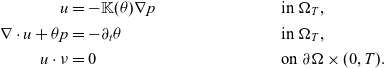 \begin{align} u &= -\mathbb{K}(\theta)\nabla p && \text{in }\Omega_T ,\notag\\ \nabla\cdot u + \theta p &= -\partial_t \theta && \text{in }\Omega_T ,\notag\\ u\cdot \nu &= 0 && \text{on } \partial\Omega\times (0,T) .\end{align}
Second, we consider the transport equation for a concentration c.
Model 2 (Transport model)
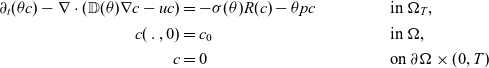 \begin{align} \partial_t(\theta c) - \nabla\cdot(\mathbb{D}(\theta)\nabla c - uc) &= - \sigma(\theta)R(c) - \theta pc && \text{in }\Omega_T ,\notag\\ c(\,.\,,0) &= c_0 && \text{in } \Omega ,\notag\\ c &= 0 && \text{on } \partial\Omega\times (0,T)\end{align}
with diffusion $\mathbb{D}(\theta)$
and reaction rate
$\mathbb{D}(\theta)$
and reaction rate $\sigma(\theta)R(c)$
.
$\sigma(\theta)R(c)$
.
In the underlying coupled model (2.1)–(2.2), we are seeking for a tuple of solution functions (c, u, p) for given porosity $\theta$
and initial data
$\theta$
and initial data $c_0$
. We apply homogeneous Dirichlet boundary conditions for the concentration field and homogeneous Neumann boundary condition for the flow problem. However, also further boundary conditions may be used as already discussed in [Reference Arbogast and Taicher3] in the context of degenerating fluid flow.
$c_0$
. We apply homogeneous Dirichlet boundary conditions for the concentration field and homogeneous Neumann boundary condition for the flow problem. However, also further boundary conditions may be used as already discussed in [Reference Arbogast and Taicher3] in the context of degenerating fluid flow.
Remark 1 The stabilising pressure term $\theta p$
in the flow equation (2.1) naturally arises in models related to mantle dynamics from the pressure differences between fluid and matrix phase which is the driving force for compaction, cf. [Reference Arbogast and Taicher3, Reference Katz15] and references cited therein. Note that in case of vanishing porosity this term is essential for the model’s analysis as performed in [Reference Arbogast and Taicher3], where a stabilised variational formulation was used to control the
$\theta p$
in the flow equation (2.1) naturally arises in models related to mantle dynamics from the pressure differences between fluid and matrix phase which is the driving force for compaction, cf. [Reference Arbogast and Taicher3, Reference Katz15] and references cited therein. Note that in case of vanishing porosity this term is essential for the model’s analysis as performed in [Reference Arbogast and Taicher3], where a stabilised variational formulation was used to control the $L^2$
-norm of
$L^2$
-norm of $\theta^{\frac{1}{2}}p$
and hence to prove existence of a solution to the flow problem, cf. Theorem 3.1 below. To balance all terms occurring in (2.1) also in the transport equation and to conduct its analysis, it is necessary to likewise include the term
$\theta^{\frac{1}{2}}p$
and hence to prove existence of a solution to the flow problem, cf. Theorem 3.1 below. To balance all terms occurring in (2.1) also in the transport equation and to conduct its analysis, it is necessary to likewise include the term $\theta p c$
into the transport equation (2.2). However, the term
$\theta p c$
into the transport equation (2.2). However, the term $\theta p$
in (2.1) (and likewise its balancing term in the transport equation) can be scaled with a small parameter to suppress its physical impact. In this way, the models applicability can be extended to further applications beyond mantle dynamics.
$\theta p$
in (2.1) (and likewise its balancing term in the transport equation) can be scaled with a small parameter to suppress its physical impact. In this way, the models applicability can be extended to further applications beyond mantle dynamics.
In Models 1 and 2, the effective permeability $\mathbb{K}$
and diffusivity
$\mathbb{K}$
and diffusivity $\mathbb{D}$
are the essential model inputs since they characterise the underlying porous medium. Although they can be computed by means of auxiliary cell problems in the context of homogenisation, it remains challenging to characterise the full effective tensors in (evolving, natural) porous media. They are consequently often assumed to be represented by scalars and linear/power laws (or Kozeny–Carman type equations) in terms of the porosity are frequently used [Reference Hommel, Coltman and Class13, Reference Ray, Rupp, Schulz and Knabner24, Reference Schulz, Ray, Zech, Rupp and Knabner27]. In this work, we rely on the following
$\mathbb{D}$
are the essential model inputs since they characterise the underlying porous medium. Although they can be computed by means of auxiliary cell problems in the context of homogenisation, it remains challenging to characterise the full effective tensors in (evolving, natural) porous media. They are consequently often assumed to be represented by scalars and linear/power laws (or Kozeny–Carman type equations) in terms of the porosity are frequently used [Reference Hommel, Coltman and Class13, Reference Ray, Rupp, Schulz and Knabner24, Reference Schulz, Ray, Zech, Rupp and Knabner27]. In this work, we rely on the following
Assumption 1 The parameters $\mathbb{K},\mathbb{D}:[0,1]\to[0,\infty)$
are assumed to be scalar-valued maps depending on the porosity
$\mathbb{K},\mathbb{D}:[0,1]\to[0,\infty)$
are assumed to be scalar-valued maps depending on the porosity $\theta$
, such that
$\theta$
, such that $\mathbb{K}(\theta)>0,\mathbb{D}(\theta)>0$
for
$\mathbb{K}(\theta)>0,\mathbb{D}(\theta)>0$
for $\theta\neq 0$
and degenerate in the sense that
$\theta\neq 0$
and degenerate in the sense that $\mathbb{K}(\theta)=\mathbb{D}(\theta)=0$
for
$\mathbb{K}(\theta)=\mathbb{D}(\theta)=0$
for $\theta=0$
. Moreover, we assume that the diffusivity satisfies the constitutive law
$\theta=0$
. Moreover, we assume that the diffusivity satisfies the constitutive law $\mathbb{D}(\theta)=\theta^d$
and likewise the permeability satisfies
$\mathbb{D}(\theta)=\theta^d$
and likewise the permeability satisfies $\mathbb{K}(\theta)=\theta^k $
. In the following we assume
$\mathbb{K}(\theta)=\theta^k $
. In the following we assume $d=1$
, i.e.
$d=1$
, i.e. $\mathbb{D}(\theta)=\theta$
, and
$\mathbb{D}(\theta)=\theta$
, and $k\geq 3$
.
$k\geq 3$
.
Remark 2 It is often assumed that the diffusivity satisfies the constitutive law $\mathbb{D}(\theta)=\alpha\theta^d$
[Reference Currie8, Reference Ray, Rupp, Schulz and Knabner24]. For instance Penman suggests
$\mathbb{D}(\theta)=\alpha\theta^d$
[Reference Currie8, Reference Ray, Rupp, Schulz and Knabner24]. For instance Penman suggests $d=1$
and
$d=1$
and $\alpha=0.66$
[Reference Penman19], while with
$\alpha=0.66$
[Reference Penman19], while with $\alpha=1$
Buckingham proposes
$\alpha=1$
Buckingham proposes $d=2$
[Reference Buckingham7], Marshall
$d=2$
[Reference Buckingham7], Marshall $d=\frac{3}{2}$
[Reference Marshall17] and Millington
$d=\frac{3}{2}$
[Reference Marshall17] and Millington $d=4/3$
[Reference Millington18]. The case
$d=4/3$
[Reference Millington18]. The case $d<1$
is on the contrary not of interest for applications since there exist the following analytically derived bounds: the Voigt–Reiss bound
$d<1$
is on the contrary not of interest for applications since there exist the following analytically derived bounds: the Voigt–Reiss bound $\mathbb{D}(\theta)\lesssim \theta$
and the n-dimensional Hashin–Shtrikman bound
$\mathbb{D}(\theta)\lesssim \theta$
and the n-dimensional Hashin–Shtrikman bound $\mathbb{D}(\theta)\lesssim \frac{n-1}{n-\theta}\theta$
for the effective diffusion, cf. [Reference Jikov, Kozlov and Oleinik14, Reference Ray, Rupp, Schulz and Knabner24]. In particular, for small porosities the three-dimensional upper Hashin–Shtrikman bound
$\mathbb{D}(\theta)\lesssim \frac{n-1}{n-\theta}\theta$
for the effective diffusion, cf. [Reference Jikov, Kozlov and Oleinik14, Reference Ray, Rupp, Schulz and Knabner24]. In particular, for small porosities the three-dimensional upper Hashin–Shtrikman bound $\frac{2}{3-\theta}\theta$
is approximated linearly by
$\frac{2}{3-\theta}\theta$
is approximated linearly by $\frac{2}{3}\theta\approx 0.66\theta$
, which is exactly the relation proposed by Penman. Hence the specific choice of
$\frac{2}{3}\theta\approx 0.66\theta$
, which is exactly the relation proposed by Penman. Hence the specific choice of $d=1$
provides a reasonable relation for small porosities. This is exactly the focus of our research since in the limit of clogging, the porosity
$d=1$
provides a reasonable relation for small porosities. This is exactly the focus of our research since in the limit of clogging, the porosity $\theta$
vanishes.
$\theta$
vanishes.
Remark 3 Well-established functional relations between the permeability and the porosity are power law relations $\mathbb{K}(\theta)\sim\theta^k $
(Verma–Pruess) and the Kozeny–Carman equation
$\mathbb{K}(\theta)\sim\theta^k $
(Verma–Pruess) and the Kozeny–Carman equation $\mathbb{K}(\theta)\sim\frac{\theta^3}{(1-\theta)^2}$
[Reference Hommel, Coltman and Class13, Reference Schulz, Ray, Zech, Rupp and Knabner27]. Since the denominator is negligible for small porosities, the Kozeny–Carman equation reduces to a power law with exponent
$\mathbb{K}(\theta)\sim\frac{\theta^3}{(1-\theta)^2}$
[Reference Hommel, Coltman and Class13, Reference Schulz, Ray, Zech, Rupp and Knabner27]. Since the denominator is negligible for small porosities, the Kozeny–Carman equation reduces to a power law with exponent $k=3$
. However, even much higher exponents are given in the literature based on experimental findings for different processes (e.g.
$k=3$
. However, even much higher exponents are given in the literature based on experimental findings for different processes (e.g. $k\geq 10$
for chemical alteration,
$k\geq 10$
for chemical alteration, $k\geq 20$
for mineral dissolution). Especially, a plenty of dissolution experiment data justify very high exponents up to an extreme value of
$k\geq 20$
for mineral dissolution). Especially, a plenty of dissolution experiment data justify very high exponents up to an extreme value of $k=431$
, cf. [Reference Bernabé, Mok and Evans5, Reference Hommel, Coltman and Class13]. Thereby large exponents correspond with increasingly heterogeneous dissolution structures such as fingering patterns. Consequently, we focus on the case
$k=431$
, cf. [Reference Bernabé, Mok and Evans5, Reference Hommel, Coltman and Class13]. Thereby large exponents correspond with increasingly heterogeneous dissolution structures such as fingering patterns. Consequently, we focus on the case $\mathbb{K}=\theta^k$
with
$\mathbb{K}=\theta^k$
with $k\geq 3$
. From an analytical point of view, the assumption
$k\geq 3$
. From an analytical point of view, the assumption $k\geq 3$
seems also to be necessary if
$k\geq 3$
seems also to be necessary if $d= 1$
. Then the advective term
$d= 1$
. Then the advective term $\nabla\cdot(uc)$
of the transport equation (2.2) can be handled and an appropriate energy estimate for space dimension three can be derived. In this sense, the Kozeny–Carman exponent
$\nabla\cdot(uc)$
of the transport equation (2.2) can be handled and an appropriate energy estimate for space dimension three can be derived. In this sense, the Kozeny–Carman exponent $k=3$
may represent a lower bound such that analytical results can be established.
$k=3$
may represent a lower bound such that analytical results can be established.
Additional assumptions are placed on the reaction term on the right hand side of (2):
Assumption 2 We assume that $\sigma:[0,1]\to[0,\infty)$
is a scalar-valued map depending on the porosity, such that
$\sigma:[0,1]\to[0,\infty)$
is a scalar-valued map depending on the porosity, such that $\theta^{-(1+\rho_1)}\sigma(\theta)\in L^2(0,T;L^\infty(\Omega))$
for some arbitrary small
$\theta^{-(1+\rho_1)}\sigma(\theta)\in L^2(0,T;L^\infty(\Omega))$
for some arbitrary small $\rho_1>0$
holds. Furthermore, let
$\rho_1>0$
holds. Furthermore, let $R:\mathbb{R}\to\mathbb{R}$
be a Lipschitz continuous map with Lipschitz constant
$R:\mathbb{R}\to\mathbb{R}$
be a Lipschitz continuous map with Lipschitz constant $L_R>0$
and the property
$L_R>0$
and the property $R(0)=0$
. Moreover, we assume
$R(0)=0$
. Moreover, we assume $R(c)c_-\leq C_R|c_-|^2$
with negative part
$R(c)c_-\leq C_R|c_-|^2$
with negative part $c_-=\min(0,c)$
.
$c_-=\min(0,c)$
.
Remark 4 The product structure of the reaction rate $f(\theta,c)=\sigma(\theta)R(c)$
is evident from upscaling theory [Reference van Noorden28] where
$f(\theta,c)=\sigma(\theta)R(c)$
is evident from upscaling theory [Reference van Noorden28] where $\sigma(\theta)$
denotes the specific surface and rates to what extend a heterogeneous (surface) reaction R(c) can take place. It is inherently related to the porosity and can analytically be determined for specific geometric situations such as circles, squares, or tubes [Reference Schulz, Ray, Zech, Rupp and Knabner27]. The conditions for the reaction rate are, for instance, fulfilled by (sub-)linear functions
$\sigma(\theta)$
denotes the specific surface and rates to what extend a heterogeneous (surface) reaction R(c) can take place. It is inherently related to the porosity and can analytically be determined for specific geometric situations such as circles, squares, or tubes [Reference Schulz, Ray, Zech, Rupp and Knabner27]. The conditions for the reaction rate are, for instance, fulfilled by (sub-)linear functions $R(c)\leq k_{\text{Reaction}}c$
. Likewise, the Langmuir type adsorption/Monod kinetic
$R(c)\leq k_{\text{Reaction}}c$
. Likewise, the Langmuir type adsorption/Monod kinetic $\frac{c}{1+c}$
does satisfy the assumptions, whereas Freundlich type adsorptions are excluded.
$\frac{c}{1+c}$
does satisfy the assumptions, whereas Freundlich type adsorptions are excluded.
In contrast to the non-degenerating problem, boundedness of solutions to Model 2 cannot be expected for vanishing porosity in general, cf. Remark 8 below. In order to prove analytical results nevertheless, the prescribed porosity field $\theta(t,x)$
must be subjected to stronger restrictions than in the non-degenerating situation, compare also the assumptions in [Reference Arbogast and Taicher3]:
$\theta(t,x)$
must be subjected to stronger restrictions than in the non-degenerating situation, compare also the assumptions in [Reference Arbogast and Taicher3]:
Assumption 3 We assume that the porosity $\theta:\Omega_T\to[0,1]$
is a given function which decreases in time and describes the process of diminishing pores, i.e. the sign condition
$\theta:\Omega_T\to[0,1]$
is a given function which decreases in time and describes the process of diminishing pores, i.e. the sign condition
 \begin{align*} \partial_t \theta\leq 0,\end{align*}
holds. Moreover, we assume that the porosity field and related quantities satisfy the following restrictions
-
a) $\theta^{\frac{k-3}{2}}\nabla\theta \in L^\infty(\Omega_T)$
and
$\theta^{-\frac{1}{2}}\partial_t\theta\in L^\infty(0,T;L^2(\Omega))$
$\theta^{\frac{k-3}{2}}\nabla\theta \in L^\infty(\Omega_T)$
and
$\theta^{-\frac{1}{2}}\partial_t\theta\in L^\infty(0,T;L^2(\Omega))$
-
b)
$\theta^{\frac{k-1}{2}}\partial_t\theta \in L^\infty(\Omega_T)$
-
c)
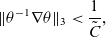
$\theta^{-1}\nabla\theta \in L^\infty(0,T;L^3(\Omega))$
fulfilling the smallness condition
$\|\theta^{-1}\nabla\theta\|_{L^\infty(L^3)}<\frac{1}{\tilde{C}}$
with an appropriate constant
$\tilde{C}>0$
, see Section 3.2.4 below -
d)
$\theta^{-1}\partial_t\theta \in L^\infty(0,T;L^3(\Omega))$


Remark 5 In order to solve the flow problem and to prove a useful integrability property of the solution Assumption a) and b) are necessary, see Theorem 3.2 and Lemma 1 below. Nevertheless, the additional conditions c)–d) are needed for the mathematical analysis of the transport model, i.e. to manage the diffusive term with $d=1$
and hence to ensure a weak solution to the transport model. In fact, the above conditions, particularly c) and d), are quite restrictive. However, the restrictions on the porosity which must be satisfied according to Assumption 3, do not intersect in an empty set. Obviously, the classical non-degenerating problem is integrated in our model by assuming non-vanishing porosity
$d=1$
and hence to ensure a weak solution to the transport model. In fact, the above conditions, particularly c) and d), are quite restrictive. However, the restrictions on the porosity which must be satisfied according to Assumption 3, do not intersect in an empty set. Obviously, the classical non-degenerating problem is integrated in our model by assuming non-vanishing porosity $\theta$
. A further more interesting example is given by
$\theta$
. A further more interesting example is given by $\theta(x,t):=e^{c\ln^{\frac{1}{3}}(|x|)}$
within the domain
$\theta(x,t):=e^{c\ln^{\frac{1}{3}}(|x|)}$
within the domain $\Omega_T=B\times(0,\frac{1}{2})$
,
$\Omega_T=B\times(0,\frac{1}{2})$
, $B:=\{y\in\mathbb{R}^3:|y|\leq \frac{1}{2}\}$
, which vanishes for
$B:=\{y\in\mathbb{R}^3:|y|\leq \frac{1}{2}\}$
, which vanishes for $x\to 0$
. Then,
$x\to 0$
. Then, $\theta$
fulfills
$\theta$
fulfills $\|\theta^{-1}\nabla\theta\|_3<\infty$
since
$\|\theta^{-1}\nabla\theta\|_3<\infty$
since
 \begin{equation*}(\theta^{-1}\nabla\theta)(x,t)=\frac{c}{3|x|\ln^{\frac{2}{3}}(|x|)}\cdot \frac{x}{|x|} \quad\text{and hence }\quad \|\theta^{-1}\nabla\theta\|_3^3=\frac{c^3}{27}\int_0^{\frac{1}{2}}\frac{dr}{r\ln^2(r)} <\infty.\end{equation*}
Although not even the gradient $\nabla\theta$
itself is bounded, the singularity is still sufficiently integrable when we multiply it with the weight
$\nabla\theta$
itself is bounded, the singularity is still sufficiently integrable when we multiply it with the weight $\theta^{-1}$
. Thereby, the smallness condition in c) can be ensured by an appropriate choice of
$\theta^{-1}$
. Thereby, the smallness condition in c) can be ensured by an appropriate choice of $c>0$
. Since
$c>0$
. Since $\theta$
does not depend on time Assumption d) is trivially fulfilled.
$\theta$
does not depend on time Assumption d) is trivially fulfilled.
3 Analysis for model
In this section, we introduce transformed variables following [Reference Arbogast and Taicher3] and proof the existence of unique, non-negative, weak solutions to Model 1 and 2.
3.1 Analysis for Darcy’s law
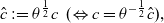
For Darcy’s law as stated in (2.1), the theory developed in [Reference Arbogast and Taicher3] directly applies. Along these lines, we consider the transformations
 \begin{equation} \hat{u}:=\mathbb{K}(\theta)^{-\frac{1}{2}}u \ \ (\Leftrightarrow u=\mathbb{K}(\theta)^{\frac{1}{2}}\hat{u})\quad \text{ and }\quad \hat{p} := \theta^{\frac{1}{2}}p \ \ (\Leftrightarrow p = \theta^{-\frac{1}{2}}\hat{p}).\end{equation}
This leads to the following scaled Darcy law including the transformed stabilising term $\theta^{\frac{1}{2}}\hat{p}$
Model 3 (Transformed flow model)
 \begin{align} \hat{u} &= -\mathbb{K}(\theta)^{\frac{1}{2}}\nabla (\theta^{-\frac{1}{2}}\hat{p}) && \text{in }\Omega_T,\end{align}
 \begin{align} \nabla\cdot(\mathbb{K}(\theta)^{\frac{1}{2}}\hat{u}) + \theta^{\frac{1}{2}}\hat{p} &= -\partial_t\theta && \text{in }\Omega_T,\end{align}
 \begin{align} \mathbb{K}(\theta)^{\frac{1}{2}}\hat{u}\cdot \nu &= 0 && \text{on } \partial\Omega\times (0,T).\end{align}
In order to define weak solutions to (3.2), we introduce the Hilbert spaces [Reference Arbogast and Taicher3]
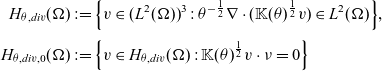 \begin{align*}H_{\theta,div}(\Omega) & := \Big\{v\in (L^2(\Omega))^{3}:\theta^{-\frac{1}{2}}\nabla\cdot(\mathbb{K}(\theta)^{\frac{1}{2}}v)\in L^2(\Omega)\Big\},\\[3pt] H_{\theta,div,0}(\Omega) & := \Big\{v\in H_{\theta,div}(\Omega): \mathbb{K}(\theta)^{\frac{1}{2}}v\cdot\nu=0 \Big\}\end{align*}
equipped with the inner product
 \begin{equation*}(u,v)_{H_{\theta,div}} = (u,v)_2 + \left(\theta^{-\frac{1}{2}}\nabla\cdot(\mathbb{K}(\theta)^{\frac{1}{2}}u)\,,\, \theta^{-\frac{1}{2}}\nabla\cdot(\mathbb{K}(\theta)^{\frac{1}{2}}v)\right)_2 ,\end{equation*}
where $(\,.\,,\,.\,)_2$
denotes the standard inner product of
$(\,.\,,\,.\,)_2$
denotes the standard inner product of $L^2(\Omega)$
. The boundary condition
$L^2(\Omega)$
. The boundary condition $\mathbb{K}(\theta)^{\frac{1}{2}}v\cdot\nu=0$
is actually given via a well-defined
$\mathbb{K}(\theta)^{\frac{1}{2}}v\cdot\nu=0$
is actually given via a well-defined $\theta$
-weighted trace operator
$\theta$
-weighted trace operator $\gamma_\theta:H_{\theta,div}(\Omega)\to H^{-\frac{1}{2}}(\partial\Omega)$
, which is defined similarly to [Reference Arbogast and Taicher3, (3.6)].
$\gamma_\theta:H_{\theta,div}(\Omega)\to H^{-\frac{1}{2}}(\partial\Omega)$
, which is defined similarly to [Reference Arbogast and Taicher3, (3.6)].
Definition 3.1 We call a pair of functions $(\hat{u},\hat{p})\in H_{\theta,div,0}(\Omega)\times L^2(\Omega)$
a weak solution to Model 3 if its weak formulation
$(\hat{u},\hat{p})\in H_{\theta,div,0}(\Omega)\times L^2(\Omega)$
a weak solution to Model 3 if its weak formulation
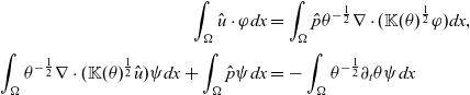 \begin{align*} \int_\Omega \hat{u} \cdot\varphi dx &= \int_\Omega \hat{p} \theta^{-\frac{1}{2}}\nabla\cdot(\mathbb{K}(\theta)^{\frac{1}{2}} \varphi) dx ,\\[3pt] \int_\Omega \theta^{-\frac{1}{2}}\nabla\cdot (\mathbb{K}(\theta)^{\frac{1}{2}}\hat{u})\psi dx + \int_\Omega\hat{p}\psi dx&= -\int_\Omega\theta^{-\frac{1}{2}}\partial_t \theta \psi dx\end{align*}
is fulfilled for test functions $\varphi\in H_{\theta,div,0}(\Omega)$
,
$\varphi\in H_{\theta,div,0}(\Omega)$
, $\psi\in L^2(\Omega)$
.
$\psi\in L^2(\Omega)$
.
Then, the following theorem holds [Reference Arbogast and Taicher3]:
Theorem 3.2 (Existence flow problem)Let Assumption 3, a) be satisfied. Then there exists a unique weak solution $(\hat{u},\hat{p})\in H_{\theta,div,0}(\Omega)\times L^2(\Omega)$
to the flow problem (3.2) and the following energy estimates holds for some
$(\hat{u},\hat{p})\in H_{\theta,div,0}(\Omega)\times L^2(\Omega)$
to the flow problem (3.2) and the following energy estimates holds for some $C>0$
:
$C>0$
:
 \begin{align} \|\hat{u}\|_2 + \|\hat{p}\|_2 + \|\theta^{-\frac{1}{2}}\nabla\cdot(\mathbb{K}(\theta)^{\frac{1}{2}}\hat{u})\|_2 \leq C \|\theta^{-\frac{1}{2}}\partial_t\theta\|_2 . \end{align}
The transformation (3.1) is necessary since the problem (3.2) can then be considered with respect to the appropriately weighted Hilbert space $H_{\theta,div}(\Omega)$
. Then, elliptic theory yields the existence of a weak solution, cf. [Reference Arbogast and Taicher3]. Nevertheless, in the transport problem, we always work with the non-transformed velocity and pressure field for the sake of readability. Backtransformation of (3.4) leads to the following energy estimate for the original unknowns (u, p):
$H_{\theta,div}(\Omega)$
. Then, elliptic theory yields the existence of a weak solution, cf. [Reference Arbogast and Taicher3]. Nevertheless, in the transport problem, we always work with the non-transformed velocity and pressure field for the sake of readability. Backtransformation of (3.4) leads to the following energy estimate for the original unknowns (u, p):
 \begin{align} \|\mathbb{K}(\theta)^{-\frac{1}{2}} u\|_2 + \|\theta^{\frac{1}{2}} p\|_2 + \|\theta^{-\frac{1}{2}}\nabla\cdot u \|_2 \leq C\|\theta^{-\frac{1}{2}}\partial_t \theta\|_2 .\end{align}
Remark 6 We note that for clogging pores the fluid flow vanishes. Contrarily, the pressure itself may be unbounded, but does not blow up worse than $\theta^{-\frac{1}{2}}$
.
$\theta^{-\frac{1}{2}}$
.
3.1.1 Integrability of u
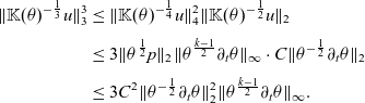
Investigating the transport equation in Section 3.2 below, we need more regularity for u. Therefore, we prove
Lemma 1 ( $\textbf{\textit{L}}^{\textbf{4}}$
-Integrability of the velocity)Let Assumption 3, b) be satisfied, then weak solutions of the flow problem (Model 1) fulfill
$\textbf{\textit{L}}^{\textbf{4}}$
-Integrability of the velocity)Let Assumption 3, b) be satisfied, then weak solutions of the flow problem (Model 1) fulfill
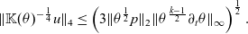 \begin{equation}\|\mathbb{K}(\theta)^{-\frac{1}{4}}u\|_4\leq\left(3\|\theta^{\frac{1}{2}}p\|_2\|\theta^{\frac{k-1}{2}}\partial_t\theta\|_\infty\right)^{\frac{1}{2}} .\end{equation}
Proof. We consider the weak formulation
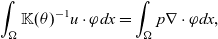 \begin{align} \int_\Omega \mathbb{K}(\theta)^{-1} u \cdot\varphi dx &= \int_\Omega p \nabla\cdot\varphi dx , \end{align}
 \begin{align} \int_\Omega \nabla\cdot u\psi dx + \int_\Omega\theta p\psi dx &= -\int_\Omega\partial_t \theta \psi dx \end{align}
of the non-transformed flow problem (Model 1). We test (3.7a) with $|u|^{2}u$
. This directly proves the lemma’s statement since
$|u|^{2}u$
. This directly proves the lemma’s statement since
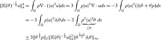 \begin{align*}\|\mathbb{K}(\theta)^{-\frac{1}{4}}u\|_4^4&=\int_\Omega p\nabla\cdot(|u|^2u) dx= 3\int_\Omega p|u|^2\nabla\cdot u dx= -3\int_\Omega p|u|^2(\partial_t\theta+\theta p)dx\\[3pt]&=-3\int_\Omega p|u|^2\partial_t\theta dx - 3\int_\Omega \underbrace{ p^2|u|^2\theta}_{\geq0}dx\\[3pt]&\leq 3\|\theta^{\frac{1}{2}}p\|_2\|\mathbb{K}(\theta)^{-\frac{1}{4}}u\|_4^2\|\theta^{\frac{k-1}{2}}\partial_t\theta\|_\infty .\end{align*}
Here, we used (3.7b), $\mathbb{K}(\theta)=\theta^k$
, cf. Assumption 1, and the regularity of p according to (3.5) (Theorem 3.2).
$\mathbb{K}(\theta)=\theta^k$
, cf. Assumption 1, and the regularity of p according to (3.5) (Theorem 3.2).
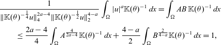
Theorem 3.3 (Integrability of the velocity)Let the conditions of Theorem 3.5 and Lemma 1 be satisfied. Then there holds for each $a\in(2,4)$
the weighted estimate
$a\in(2,4)$
the weighted estimate
 \begin{equation}\|\mathbb{K}(\theta)^{-\frac{1}{a}}u\|_a^a\leq \|\mathbb{K}(\theta)^{-\frac{1}{4}}u\|_4^{2a-4}\|\mathbb{K}(\theta)^{-\frac{1}{2}}u\|_2^{4-a} <\infty .\end{equation}
Proof. We combine Lemma 1 with the non-transformed energy estimate (3.5) to prove the boundedness of $\|\mathbb{K}(\theta)^{-\frac{1}{a}}u\|_a$
with
$\|\mathbb{K}(\theta)^{-\frac{1}{a}}u\|_a$
with $a\in(2,4)$
via a weighted estimate of Lyapunov type: To this end, we define
$a\in(2,4)$
via a weighted estimate of Lyapunov type: To this end, we define
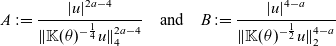 \begin{equation*}A:=\frac{|u|^{2a-4}}{\|\mathbb{K}(\theta)^{-\frac{1}{4}}u\|_4^{2a-4}}\quad\text{and}\quad B:=\frac{|u|^{4-a}}{\|\mathbb{K}(\theta)^{-\frac{1}{2}}u\|_2^{4-a}}\end{equation*}
and apply Young’s inequality (with $\frac{2a-4}{4}+\frac{4-a}{2}=1$
) to obtain
$\frac{2a-4}{4}+\frac{4-a}{2}=1$
) to obtain $AB\leq \frac{2a-4}{4}A^{\frac{4}{2a-4}}+\frac{4-a}{2}B^{\frac{2}{4-a}}$
. Multiplying AB with
$AB\leq \frac{2a-4}{4}A^{\frac{4}{2a-4}}+\frac{4-a}{2}B^{\frac{2}{4-a}}$
. Multiplying AB with $\mathbb{K}(\theta)^{-1}$
and integrating actually leads to
$\mathbb{K}(\theta)^{-1}$
and integrating actually leads to
 \begin{align*}&\frac{1}{\|\mathbb{K}(\theta)^{-\frac{1}{4}}u\|_4^{2a-4}\|\mathbb{K}(\theta)^{-\frac{1}{2}}u\|_2^{4-a}}\int_\Omega |u|^a\mathbb{K}(\theta)^{-1}\,dx =\int_\Omega AB\,\mathbb{K}(\theta)^{-1}\,dx\\[3pt]&\qquad \leq \frac{2a-4}{4}\int_\Omega A^{\frac{4}{2a-4}}\mathbb{K}(\theta)^{-1}\,dx+\frac{4-a}{2}\int_\Omega B^{\frac{2}{4-a}}\mathbb{K}(\theta)^{-1}\,dx=1 ,\end{align*}
which directly implies the assertion.
In particular, we are interested in an estimate choosing $a=3$
in (3.8) and hence consider in this special situation the upper bound in more detail. Thereby we obtain with (3.5) and (3.6)
$a=3$
in (3.8) and hence consider in this special situation the upper bound in more detail. Thereby we obtain with (3.5) and (3.6)
 \begin{align}\|\mathbb{K}(\theta)^{-\frac{1}{3}}u\|_3^3 &\leq \|\mathbb{K}(\theta)^{-\frac{1}{4}}u\|_4^2\|\mathbb{K}(\theta)^{-\frac{1}{2}}u\|_2\notag\\[3pt]&\leq 3\|\theta^{\frac{1}{2}}p\|_2\|\theta^{\frac{k-1}{2}}\partial_t\theta\|_\infty\cdot C\|\theta^{-\frac{1}{2}}\partial_t \theta\|_2\notag\\[3pt]&\leq 3C^2\|\theta^{-\frac{1}{2}}\partial_t \theta\|_2^2\|\theta^{\frac{k-1}{2}}\partial_t\theta\|_\infty .\end{align}
Since we investigated an elliptic equation during this section, we dropped the time-dependence of $\theta$
and hence of the solution
$\theta$
and hence of the solution $(\hat{u},\hat{p})$
. The flow model in (2.1) is of stationary type and depends on time only due to
$(\hat{u},\hat{p})$
. The flow model in (2.1) is of stationary type and depends on time only due to $\theta$
, i.e. the integrability of
$\theta$
, i.e. the integrability of $(\hat{u},\hat{p})$
with respect to time is inherited fromAssumption 3:
$(\hat{u},\hat{p})$
with respect to time is inherited fromAssumption 3:
 \begin{equation*}\hat{u}\in L^\infty(0,T;H_{\theta,div,0}(\Omega)) \quad{and}\quad \hat{p}\in L^\infty(0,T;L^2(\Omega)) .\end{equation*}
For the same reason we have $\mathbb{K}(\theta)^{-\frac{1}{a}}u\in L^\infty(0,T;L^a(\Omega))$
for all
$\mathbb{K}(\theta)^{-\frac{1}{a}}u\in L^\infty(0,T;L^a(\Omega))$
for all $a\in[2,4]$
.
$a\in[2,4]$
.
3.2 Analysis for the transport equation
3.2.1 Transformation and function spaces for the transport equation
In this section, we analyse the transport problem, cf. Model 2. Similar to the transformation of the velocity and pressure given in Section 3.1, we define the transformation of the concentration field
 \begin{align*}\hat{c}:=\theta^{\frac{1}{2}}c \ \ (\Leftrightarrow c = \theta^{-\frac{1}{2}}\hat{c}) ,\end{align*}
such that we are again able to analytically handle the corresponding problem by the introduction of an appropriate weighted function space.
The scaled transport equation reads
 \begin{align} \partial_t(\theta^{\frac{1}{2}} \hat{c}) - \nabla\cdot(\mathbb{D}\nabla (\theta^{-\frac{1}{2}}\hat{c}) -\theta^{-\frac{1}{2}}u\hat{c}) &= -\sigma(\theta)\hat{R}(\hat{c}) - \theta^{\frac{1}{2}}p\hat{c} && \text{in }\Omega_T ,\end{align}
 \begin{align} \hat{c}&=0 && \text{on }\partial\Omega \times (0,T) ,\end{align}
 \begin{align} \hat{c}(\,.\,,0)&=\hat{c}_0 && \text{in } \Omega ,\end{align}
where $\hat{R}(\hat{c}):=R(\theta^{-\frac{1}{2}}\hat{c})=R(c)$
for the given porosity function
$\hat{R}(\hat{c}):=R(\theta^{-\frac{1}{2}}\hat{c})=R(c)$
for the given porosity function $\theta$
and
$\theta$
and $\hat{c}_0:=\theta(\,.\,,0)^{\frac{1}{2}}c_0$
. Due to the Lipschitz continuity of R and
$\hat{c}_0:=\theta(\,.\,,0)^{\frac{1}{2}}c_0$
. Due to the Lipschitz continuity of R and $R(0)=0$
, the transformed reaction rate function
$R(0)=0$
, the transformed reaction rate function $\hat{R}$
satisfies the condition
$\hat{R}$
satisfies the condition
 \begin{equation}\hat{R}(\hat{c})\leq L_R\theta^{-\frac{1}{2}}|\hat{c}| .\end{equation}
Inspired by the energy estimate, cf. Theorem 3.3, and [Reference Arbogast and Taicher3], we consider the function space
 \begin{align*} V_0(\Omega):=\Big\{\zeta\in L^2(\Omega): \mathbb{D}(\theta)^{\frac{1}{2}}\nabla (\theta^{-\frac{1}{2}}\zeta)\in (L^2(\Omega))^{3}\ \text{and}\ \zeta=0\ \text{on }\partial\Omega\Big\} .\end{align*}
We remark that due to $\theta$
the function space
$\theta$
the function space $V_0(\Omega)$
is time-dependent although it describes the spatial dependence of an unknown. The corresponding inner product is given by
$V_0(\Omega)$
is time-dependent although it describes the spatial dependence of an unknown. The corresponding inner product is given by
 \begin{align}(\zeta,\eta)_{V_0}:= (\zeta,\eta)_2 + \left( \mathbb{D}(\theta)^{\frac{1}{2}}\nabla (\theta^{-\frac{1}{2}}\zeta)\,,\, \mathbb{D}(\theta)^{\frac{1}{2}}\nabla (\theta^{-\frac{1}{2}}\eta)\right)_2 ,\end{align}
cf. [Reference Arbogast and Taicher3] and we conclude
Lemma 2 Let the condition of Assumption 3, c) on $\theta$
be satisfied. Then, the space
$\theta$
be satisfied. Then, the space $V_0(\Omega)$
equipped with the inner product
$V_0(\Omega)$
equipped with the inner product $(\,.\,,\,.\,)_{V_0}$
defined in (3.12) is a Hilbert space.
$(\,.\,,\,.\,)_{V_0}$
defined in (3.12) is a Hilbert space.
Proof. Since this is a special case of the situation discussed in [Reference Arbogast and Taicher3], we follow the proof of [Reference Arbogast and Taicher3, Lemma 3.1] and it suffices to verify the completeness of $V_0(\Omega)$
. Thus, let
$V_0(\Omega)$
. Thus, let $(u_k)_{k\in\mathbb{N}}\subset V_0(\Omega)$
be a Cauchy sequence, i.e.
$(u_k)_{k\in\mathbb{N}}\subset V_0(\Omega)$
be a Cauchy sequence, i.e.
 \begin{equation*}\|u_k-u_n\|_{V_0}^2=\|u_k-u_n\|_2^2+\|\mathbb{D}(\theta)^{\frac{1}{2}}\nabla(\theta^{-\frac{1}{2}}(u_k-u_n))\|_2^2\ \stackrel{k,n\to\infty}{\longrightarrow}\ 0 .\end{equation*}
The completeness of $L^2(\Omega)$
implies the convergence of the sequences
$L^2(\Omega)$
implies the convergence of the sequences $(u_k)_{k\in\mathbb{N}}$
and
$(u_k)_{k\in\mathbb{N}}$
and $(\mathbb{D}(\theta)^{\frac{1}{2}}\nabla (\theta^{-\frac{1}{2}} u_k))_{k\in\mathbb{N}}$
in
$(\mathbb{D}(\theta)^{\frac{1}{2}}\nabla (\theta^{-\frac{1}{2}} u_k))_{k\in\mathbb{N}}$
in $L^2(\Omega)$
, i.e.
$L^2(\Omega)$
, i.e. $u_k\rightarrow u\in L^2(\Omega)$
and
$u_k\rightarrow u\in L^2(\Omega)$
and $\mathbb{D}(\theta)^{\frac{1}{2}}\nabla (\theta^{-\frac{1}{2}} u_k)\rightarrow\psi\in L^2(\Omega)$
as
$\mathbb{D}(\theta)^{\frac{1}{2}}\nabla (\theta^{-\frac{1}{2}} u_k)\rightarrow\psi\in L^2(\Omega)$
as $k\to\infty$
. Testing the sequence
$k\to\infty$
. Testing the sequence $(\mathbb{D}(\theta)^{\frac{1}{2}}\nabla (\theta^{-\frac{1}{2}}u_k))_{k\in\mathbb{N}}$
with a smooth function
$(\mathbb{D}(\theta)^{\frac{1}{2}}\nabla (\theta^{-\frac{1}{2}}u_k))_{k\in\mathbb{N}}$
with a smooth function $\phi\in C_0^\infty(\Omega)$
yields
$\phi\in C_0^\infty(\Omega)$
yields
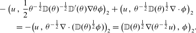
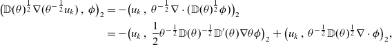 \begin{align*}\big(\mathbb{D}(\theta)^{\frac{1}{2}}\nabla (\theta^{-\frac{1}{2}} u_k)\,,\,\phi\big)_2 &= -\big(u_k\,,\,\theta^{-\frac{1}{2}}\nabla\cdot(\mathbb{D}(\theta)^{\frac{1}{2}}\phi)\big)_2\\&= -\big(u_k\,,\,\frac{1}{2}\theta^{-\frac{1}{2}}\mathbb{D}(\theta)^{-\frac{1}{2}}\mathbb{D}'(\theta)\nabla\theta\phi\big)_2+\big(u_k\,,\,\theta^{-\frac{1}{2}}\mathbb{D}(\theta)^{\frac{1}{2}}\nabla\cdot\phi\big)_2 ,\end{align*}
where $\mathbb{D}(\theta)=\theta$
, cf. Assumption 1, and the condition
$\mathbb{D}(\theta)=\theta$
, cf. Assumption 1, and the condition $\theta^{-1}\nabla\theta\in L^2(\Omega)$
, cf. Assumption 3, ensures that
$\theta^{-1}\nabla\theta\in L^2(\Omega)$
, cf. Assumption 3, ensures that $\theta^{-\frac{1}{2}}\mathbb{D}(\theta)^{-\frac{1}{2}}\mathbb{D}'(\theta)\nabla\theta$
belongs to
$\theta^{-\frac{1}{2}}\mathbb{D}(\theta)^{-\frac{1}{2}}\mathbb{D}'(\theta)\nabla\theta$
belongs to $L^2(\Omega)$
. Due to the
$L^2(\Omega)$
. Due to the $L^2$
-convergence of
$L^2$
-convergence of $(u_k)_{k\in\mathbb{N}}$
the right-hand side converges to
$(u_k)_{k\in\mathbb{N}}$
the right-hand side converges to
 \begin{align*}&-\big(u\,,\,\frac{1}{2}\theta^{-\frac{1}{2}}\mathbb{D}(\theta)^{-\frac{1}{2}}\mathbb{D}'(\theta)\nabla\theta\phi\big)_2 + \big(u\,,\,\theta^{-\frac{1}{2}}\mathbb{D}(\theta)^{\frac{1}{2}}\nabla\cdot\phi\big)_2\\&\qquad =-\big(u\,,\,\theta^{-\frac{1}{2}}\nabla\cdot(\mathbb{D}(\theta)^{\frac{1}{2}}\phi)\big)_2=\big(\mathbb{D}(\theta)^{\frac{1}{2}}\nabla (\theta^{-\frac{1}{2}}u)\,,\,\phi\big)_2 .\end{align*}
Finally, we conclude $\psi=\mathbb{D}(\theta)^{\frac{1}{2}}\nabla (\theta^{-\frac{1}{2}} u)$
which completes the proof.
$\psi=\mathbb{D}(\theta)^{\frac{1}{2}}\nabla (\theta^{-\frac{1}{2}} u)$
which completes the proof.
3.2.2 Weak formulation
In this section, we introduce the weak formulation to the transformed transport equation (3.10) and consider relations between weighted and standard function spaces.
Definition 3.4 We call
 \begin{equation}\hat{c}\in \mathcal{X}_\theta:=\Big\{\zeta \in L^2(0,T;H_0^1(\Omega))\,|\,\theta^{-\frac{1}{2}}\partial_t (\theta^{\frac{1}{2}}\zeta)\in L^2(0,T;H^{-1}(\Omega))\Big\} ,\end{equation}
a weak solution to (3.10) if the scaled transport equation is fulfilled in the weak sense, i.e.
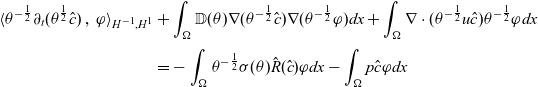 \begin{align}\langle \theta^{-\frac{1}{2}}\partial_t (\theta^{\frac{1}{2}}\hat{c})\,,\,\varphi\rangle_{H^{-1},H^1}&+ \int_\Omega\mathbb{D}(\theta)\nabla (\theta^{-\frac{1}{2}}\hat{c})\nabla(\theta^{-\frac{1}{2}}\varphi) dx+ \int_\Omega\nabla\cdot(\theta^{-\frac{1}{2}}u\hat{c})\theta^{-\frac{1}{2}}\varphi dx \notag \\[3pt]&= -\int_\Omega\theta^{-\frac{1}{2}}\sigma(\theta)\hat{R}(\hat{c})\varphi dx - \int_\Omega p\hat{c}\varphi dx\end{align}
holds for given porosity function $\theta$
, (u,p) from Section 3.1, and test functions
$\theta$
, (u,p) from Section 3.1, and test functions $\varphi\in H_0^1(\Omega)$
for a.e.
$\varphi\in H_0^1(\Omega)$
for a.e. $t\in(0,T)$
. Here
$t\in(0,T)$
. Here $\langle \,.\,,\,.\,\rangle_{H^{-1},H^1}$
denotes the standard dual product of
$\langle \,.\,,\,.\,\rangle_{H^{-1},H^1}$
denotes the standard dual product of $H^{-1}(\Omega)$
and
$H^{-1}(\Omega)$
and $H_0^1(\Omega)$
. Moreover the initial value
$H_0^1(\Omega)$
. Moreover the initial value $\hat{c}_0\in L^2(\Omega)$
is taken in the following sense
$\hat{c}_0\in L^2(\Omega)$
is taken in the following sense
 \begin{equation*}(\hat{c}(t)-\hat{c}_0,\psi)_{2}\stackrel{t\to0}{\longrightarrow}0\qquad \text{for all }\psi\in L^2(\Omega) .\end{equation*}
We now further investigate the relation between the weighted function spaces $V_0(\Omega)$
,
$V_0(\Omega)$
, $\mathcal{X}_\theta$
defined above and the standard function spaces for general
$\mathcal{X}_\theta$
defined above and the standard function spaces for general $\mathbb{D}(\theta)=\theta^d$
,
$\mathbb{D}(\theta)=\theta^d$
, $d\geq 0$
:
$d\geq 0$
:
Lemma 3 For $\mathbb{D}(\theta)^{\frac{1}{2}}\theta^{-\frac{3}{2}}\nabla\theta\in L^3(\Omega)$
, the following embeddings hold:
$\mathbb{D}(\theta)^{\frac{1}{2}}\theta^{-\frac{3}{2}}\nabla\theta\in L^3(\Omega)$
, the following embeddings hold:
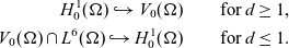 \begin{align*}H_0^1(\Omega) \hookrightarrow V_0(\Omega)\qquad & \text{for }d\geq 1 ,\\V_0(\Omega)\cap L^6(\Omega) \hookrightarrow H_0^1(\Omega)\qquad & \text{for }d\leq 1 .\end{align*}
Consequently, with Assumptions 1 and 3, c) we have the isomorphism
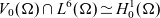 \begin{align*} V_0(\Omega)\cap L^6(\Omega)\simeq H_0^1(\Omega)\end{align*}
for a.e. $t\in(0,T)$
.
$t\in(0,T)$
.
If additionally Assumption 3, d) holds, the solution space $\mathcal{X}_\theta$
is isomorph to the standard parabolic solution space, i.e.
$\mathcal{X}_\theta$
is isomorph to the standard parabolic solution space, i.e.
 \begin{equation*}\mathcal{X}_\theta\simeq\mathcal{X}:=\Big\{\zeta\in L^2(0,T;H_0^1(\Omega))\,|\,\partial_t\zeta\in L^2(0,T;H^{-1}(\Omega))\Big\} .\end{equation*}
Proof. By the product rule, it holds for an arbitrary function $\xi:\Omega\to\mathbb{R}$
 \begin{equation} \mathbb{D}(\theta)^{\frac{1}{2}}\nabla(\theta^{-\frac{1}{2}}\xi) = \mathbb{D}(\theta)^{\frac{1}{2}}\theta^{-\frac{1}{2}}\nabla \xi -\frac{1}{2}\mathbb{D}(\theta)^{\frac{1}{2}}\theta^{-\frac{3}{2}}(\nabla \theta) \xi .\end{equation}
Assuming $\xi\in H_0^1(\Omega)$
and applying the Sobolev embedding
$\xi\in H_0^1(\Omega)$
and applying the Sobolev embedding $H^1(\Omega)\hookrightarrow L^6(\Omega)$
, it suffices that
$H^1(\Omega)\hookrightarrow L^6(\Omega)$
, it suffices that $\mathbb{D}(\theta)^{\frac{1}{2}}\theta^{-\frac{3}{2}}\nabla \theta$
belongs to
$\mathbb{D}(\theta)^{\frac{1}{2}}\theta^{-\frac{3}{2}}\nabla \theta$
belongs to $L^3(\Omega)$
and that
$L^3(\Omega)$
and that $d\geq 1$
to have the left-hand side in
$d\geq 1$
to have the left-hand side in $L^2(\Omega)$
, i.e.
$L^2(\Omega)$
, i.e. $H_0^1(\Omega)\hookrightarrow V_0(\Omega)$
. On the contrary, the embedding
$H_0^1(\Omega)\hookrightarrow V_0(\Omega)$
. On the contrary, the embedding $V_0(\Omega)\cap L^6(\Omega)\hookrightarrow H_0^1(\Omega)$
holds for
$V_0(\Omega)\cap L^6(\Omega)\hookrightarrow H_0^1(\Omega)$
holds for $d\leq1$
again due to
$d\leq1$
again due to $\mathbb{D}(\theta)^{\frac{1}{2}}\theta^{-\frac{3}{2}}\nabla \theta\in L^3(\Omega)$
.
$\mathbb{D}(\theta)^{\frac{1}{2}}\theta^{-\frac{3}{2}}\nabla \theta\in L^3(\Omega)$
.
For $\zeta\in L^2(0,T;H_0^1(\Omega))$
, we similarly have
$\zeta\in L^2(0,T;H_0^1(\Omega))$
, we similarly have
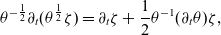 \begin{equation*}\theta^{-\frac{1}{2}}\partial_t(\theta^{\frac{1}{2}}\zeta)=\partial_t\zeta+\frac{1}{2}\theta^{-1}(\partial_t\theta)\zeta ,\end{equation*}
i.e. with $\theta^{-1}(\partial_t\theta)\in L^\infty(0,T;L^{3}(\Omega))$
the term
$\theta^{-1}(\partial_t\theta)\in L^\infty(0,T;L^{3}(\Omega))$
the term $\theta^{-1}(\partial_t)\zeta$
belongs to
$\theta^{-1}(\partial_t)\zeta$
belongs to $L^2(\Omega_T)\hookrightarrow L^2(0,T;H^{-1}(\Omega))$
and hence the following equivalence holds:
$L^2(\Omega_T)\hookrightarrow L^2(0,T;H^{-1}(\Omega))$
and hence the following equivalence holds:
 \begin{align*}\theta^{-\frac{1}{2}}\partial_t(\theta^{\frac{1}{2}}\zeta)\in L^2(0,T;H^{-1}(\Omega))\quad\Leftrightarrow\quad \partial_t\zeta\in L^2(0,T;H^{-1}(\Omega)) .\\[-40pt]\end{align*}
Remark 7 Although the transformed function spaces are isomorph to standard function spaces under specific preconditions on the coefficients and assumptions on the regularity of the given porosity field, we emphasise that all these statements refer to the transformed concentration $\hat{c}$
. These isomorphisms allow considering the problem in the time-independent spatial function space
$\hat{c}$
. These isomorphisms allow considering the problem in the time-independent spatial function space $H^1_0(\Omega)$
instead of
$H^1_0(\Omega)$
instead of $V_0(\Omega)$
. Moreover, necessary standard embeddings can be applied for the solution
$V_0(\Omega)$
. Moreover, necessary standard embeddings can be applied for the solution $\hat{c}$
. However, estimates must also be interpreted for the non-transformed concentration c in order to understand the physical complexity of the degenerating problem, compare also Remark 8.
$\hat{c}$
. However, estimates must also be interpreted for the non-transformed concentration c in order to understand the physical complexity of the degenerating problem, compare also Remark 8.
3.2.3 Regularisation
In order to prove existence of weak solutions to the degenerating model (3.10) in the sense of Definition 3.4, we consider for a regularisation parameter $\varepsilon>0$
the following non-degenerating regularisation of the transport problem
$\varepsilon>0$
the following non-degenerating regularisation of the transport problem
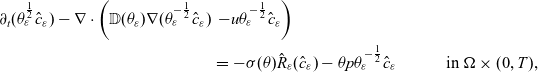 \begin{align}\partial_t (\theta_\varepsilon^{\frac{1}{2}} \hat{c}_\varepsilon) - \nabla\cdot\left(\mathbb{D}(\theta_\varepsilon)\nabla (\theta_\varepsilon^{-\frac{1}{2}} \hat{c}_\varepsilon) \right.&\left.- u \theta_\varepsilon^{-\frac{1}{2}}\hat{c}_\varepsilon\right)\notag\\&= -\sigma(\theta)\hat{R}_\varepsilon(\hat{c}_\varepsilon) - \theta p \theta_\varepsilon^{-\frac{1}{2}}\hat{c}_\varepsilon && \text{in }\Omega\times (0,T) ,\end{align}
 \begin{align} \hat{c}_\varepsilon&=0 && \text{on }\partial\Omega \times (0,T) ,\end{align}
 \begin{align} \hat{c}_\varepsilon(\,.\,,0)&=\hat{c}_0 && \text{in } \Omega\end{align}
with $\hat{R}_\varepsilon(\hat{c}_\varepsilon):=R(\theta_\varepsilon^{-\frac{1}{2}}\hat{c}_\varepsilon)$
. Moreover, the given porosity
$\hat{R}_\varepsilon(\hat{c}_\varepsilon):=R(\theta_\varepsilon^{-\frac{1}{2}}\hat{c}_\varepsilon)$
. Moreover, the given porosity $\theta$
is replaced by
$\theta$
is replaced by
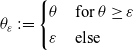 \begin{equation}\theta_\varepsilon:=\begin{cases}\theta & \text{for }\theta\geq\varepsilon\\\varepsilon & \text{else}\end{cases}\end{equation}
avoiding the porosity to fall below $\varepsilon>0$
.
$\varepsilon>0$
.
In (3.16) the weak solution (u, p) of the degenerating flow model (2.1) is defined as before, i.e. no regularisation is undertaken for these quantities. Furthermore, the argument of $\sigma(\theta)$
is not replaced by
$\sigma(\theta)$
is not replaced by $\theta_\varepsilon$
in (3.16) and the stabilisation term is specifically split to ensure the applicability of (3.7b) later on.
$\theta_\varepsilon$
in (3.16) and the stabilisation term is specifically split to ensure the applicability of (3.7b) later on.
Obviously, this system does not degenerate and hence standard parabolic theory [Reference Ladyženskaja, Solonnikov and Ural’ceva16, Chap. III] can be applied with respect to the usual function space $\mathcal{X}$
. Therefore, for each
$\mathcal{X}$
. Therefore, for each $\varepsilon>0$
we obtain a solution
$\varepsilon>0$
we obtain a solution $\hat{c}_\varepsilon\in \mathcal{X}$
.
$\hat{c}_\varepsilon\in \mathcal{X}$
.
3.2.4 Regularisation – uniform energy estimates
In this section, we derive energy estimates for solutions to the regularised model (3.16) for $\mathbb{D}(\theta)=\theta$
and the parameter choice
$\mathbb{D}(\theta)=\theta$
and the parameter choice $k\geq 3$
, cf. Assumption 1. As a consequence of (3.15) and the homogeneous Dirichlet boundary condition, the Sobolev embedding
$k\geq 3$
, cf. Assumption 1. As a consequence of (3.15) and the homogeneous Dirichlet boundary condition, the Sobolev embedding $H_0^1(\Omega)\hookrightarrow L^6(\Omega)$
(
$H_0^1(\Omega)\hookrightarrow L^6(\Omega)$
( $C_S>0$
) and the Poincare’s inequality (
$C_S>0$
) and the Poincare’s inequality ( $C_P>0$
) yield for a solution
$C_P>0$
) yield for a solution $\hat{c}_\varepsilon$
to (3.16)
$\hat{c}_\varepsilon$
to (3.16)
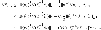 \begin{align*}\|\nabla \hat{c}_\varepsilon\|_2 & \leq \|\mathbb{D}(\theta_\varepsilon)^{\frac{1}{2}}\nabla(\theta_\varepsilon^{-\frac{1}{2}}\hat{c}_\varepsilon)\|_2+\frac{1}{2}\|\theta_\varepsilon^{-1}\nabla\theta_\varepsilon\|_3\|\hat{c}_\varepsilon\|_6\notag\\[2pt]& \leq \|\mathbb{D}(\theta_\varepsilon)^{\frac{1}{2}}\nabla(\theta_\varepsilon^{-\frac{1}{2}}\hat{c}_\varepsilon)\|_2+C_S\frac{1}{2}\|\theta_\varepsilon^{-1}\nabla\theta_\varepsilon\|_3\|\hat{c}_\varepsilon\|_{H^1}\notag\\[2pt]& \leq \|\mathbb{D}(\theta_\varepsilon)^{\frac{1}{2}}\nabla(\theta_\varepsilon^{-\frac{1}{2}}\hat{c}_\varepsilon)\|_2+C_SC_P\|\theta_\varepsilon^{-1}\nabla\theta_\varepsilon\|_3\|\nabla \hat{c}_\varepsilon\|_{2} .\end{align*}
Let us mention that due to the definition of $\theta_\varepsilon$
there holds
$\theta_\varepsilon$
there holds $\|\theta_\varepsilon^{-1}\nabla\theta_\varepsilon\|_3 \leq \|\theta^{-1}\nabla\theta\|_3$
for all
$\|\theta_\varepsilon^{-1}\nabla\theta_\varepsilon\|_3 \leq \|\theta^{-1}\nabla\theta\|_3$
for all $\varepsilon>0$
. Therefore, in case that the smallness condition
$\varepsilon>0$
. Therefore, in case that the smallness condition
 \begin{equation*} \|\theta^{-1}\nabla\theta\|_3<\frac{1}{\tilde{C}},\end{equation*}
is satisfied with $\tilde{C}:=C_SC_P$
, cf. Assumption 3 c), the gradient
$\tilde{C}:=C_SC_P$
, cf. Assumption 3 c), the gradient $\nabla\hat{c}_\varepsilon$
can be estimated uniformly by the weighted gradient
$\nabla\hat{c}_\varepsilon$
can be estimated uniformly by the weighted gradient $\mathbb{D}(\theta_\varepsilon)^{\frac{1}{2}}\nabla(\theta_\varepsilon^{-\frac{1}{2}}\hat{c}_\varepsilon)$
as follows:
$\mathbb{D}(\theta_\varepsilon)^{\frac{1}{2}}\nabla(\theta_\varepsilon^{-\frac{1}{2}}\hat{c}_\varepsilon)$
as follows:
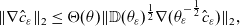 \begin{equation} \|\nabla \hat{c}_\varepsilon\|_2 \leq \Theta(\theta)\|\mathbb{D}(\theta_\varepsilon)^{\frac{1}{2}}\nabla(\theta_\varepsilon^{-\frac{1}{2}}\hat{c}_\varepsilon)\|_2, \end{equation}
with $\Theta(\theta):= \frac{1}{1-\tilde{C}\|\theta^{-1}\nabla\theta\|_{L^\infty(L^3)}}\in (1,\infty)$
.
$\Theta(\theta):= \frac{1}{1-\tilde{C}\|\theta^{-1}\nabla\theta\|_{L^\infty(L^3)}}\in (1,\infty)$
.
Since in the limit $\varepsilon\rightarrow 0$
a degenerating system is considered, it is necessary to derive uniformly bounded estimates in adequately
$\varepsilon\rightarrow 0$
a degenerating system is considered, it is necessary to derive uniformly bounded estimates in adequately $\theta$
-weighted norms:
$\theta$
-weighted norms:
Theorem 3.5 Under the Assumptions 1, 2 and 3, the condition $\hat{c}_0\in L^2(\Omega)$
, and the additional smallness assumption
$\hat{c}_0\in L^2(\Omega)$
, and the additional smallness assumption
 \begin{equation}2\tilde{C} \Theta(\theta)\|\mathbb{K}(\theta)^{-\frac{1}{3}}u\|_3\leq 2\tilde{C}\Theta(\theta)\left(3C^2\|\theta^{-\frac{1}{2}}\partial_t \theta\|_2^2\|\theta\partial_t\theta\|_\infty\right)^{\frac{1}{3}} < 1,\end{equation}
for a.e. $t\in(0,T)$
if
$t\in(0,T)$
if $k=3$
, the following uniform energy estimate holds for solutions
$k=3$
, the following uniform energy estimate holds for solutions $\hat{c}_\varepsilon$
to the regularised problem (3.16):
$\hat{c}_\varepsilon$
to the regularised problem (3.16):
 \begin{align*}\|\hat{c}_\varepsilon\|^2_{L^\infty(L^2)} + \|\mathbb{D}(\theta_\varepsilon)^{\frac{1}{2}}\nabla (\theta^{-\frac{1}{2}}_\varepsilon \hat{c}_\varepsilon)\|^2_{L^2(L^2)} + \|\theta^{-\frac{1}{2}}_\varepsilon\partial_t(\theta^{\frac{1}{2}}_\varepsilon \hat{c}_\varepsilon)\|_{L^2(H^{-1})}^2 <\infty .\end{align*}
Proof. We test equation (3.16) with $\theta_\varepsilon^{-\frac{1}{2}}\hat{c}_\varepsilon$
and apply (3.7b) as well as (3.11) to obtain the energy estimate:
$\theta_\varepsilon^{-\frac{1}{2}}\hat{c}_\varepsilon$
and apply (3.7b) as well as (3.11) to obtain the energy estimate:
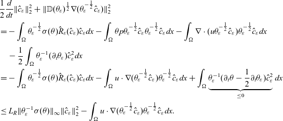 \begin{align*} &\frac{1}{2}\frac{d}{dt}\|\hat{c}_\varepsilon\|^2_2 + \|\mathbb{D}(\theta_\varepsilon)^{\frac{1}{2}}\nabla (\theta_\varepsilon^{-\frac{1}{2}}\hat{c}_\varepsilon)\|^2_2 \\[2pt] &=- \int_\Omega \theta_\varepsilon^{-\frac{1}{2}}\sigma(\theta)\hat{R}_\varepsilon(\hat{c}_\varepsilon)\hat{c}_\varepsilon dx -\int_\Omega \theta p\theta_\varepsilon^{-\frac{1}{2}}\hat{c}_\varepsilon\theta_\varepsilon^{-\frac{1}{2}}\hat{c}_\varepsilon dx - \int_\Omega \nabla\cdot(u\theta_\varepsilon^{-\frac{1}{2}}\hat{c}_\varepsilon)\theta_\varepsilon^{-\frac{1}{2}}\hat{c}_\varepsilon dx\\[3pt] &\quad - \frac{1}{2}\int_\Omega\theta_\varepsilon^{-1}(\partial_t\theta_\varepsilon) \hat{c}_\varepsilon^2 dx\\ &=- \int_\Omega \theta_\varepsilon^{-\frac{1}{2}}\sigma(\theta)\hat{R}_\varepsilon(\hat{c}_\varepsilon)\hat{c}_\varepsilon dx - \int_\Omega u\cdot\nabla (\theta_\varepsilon^{-\frac{1}{2}}\hat{c}_\varepsilon)\theta_\varepsilon^{-\frac{1}{2}}\hat{c}_\varepsilon dx + \int_\Omega \underbrace{\theta_\varepsilon^{-1}(\partial_t\theta-\frac{1}{2}\partial_t\theta_\varepsilon) \hat{c}_\varepsilon^2}_{\leq0} dx\\& \leq L_R \|\theta_\varepsilon^{-1}\sigma(\theta)\|_\infty\|\hat{c}_\varepsilon\|_2^2 - \int_\Omega u\cdot\nabla (\theta_\varepsilon^{-\frac{1}{2}}\hat{c}_\varepsilon)\theta_\varepsilon^{-\frac{1}{2}}\hat{c}_\varepsilon dx . \end{align*}
For the last estimate, we used the fact that $\partial_t\theta-\frac{1}{2}\partial_t\theta_\varepsilon\leq0$
due to the definition of
$\partial_t\theta-\frac{1}{2}\partial_t\theta_\varepsilon\leq0$
due to the definition of $\theta_\varepsilon$
, cf. (3.17) and Assumption 3. The last term on the right-hand side must be absorbed into the weighted diffusive term, which is possible due to the integrability of the velocity, see Section 3.1.1. More precisely, to manage the integral
$\theta_\varepsilon$
, cf. (3.17) and Assumption 3. The last term on the right-hand side must be absorbed into the weighted diffusive term, which is possible due to the integrability of the velocity, see Section 3.1.1. More precisely, to manage the integral
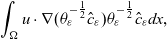 \begin{equation}\int_\Omega u\cdot\nabla (\theta_\varepsilon^{-\frac{1}{2}}\hat{c}_\varepsilon)\theta_\varepsilon^{-\frac{1}{2}}\hat{c}_\varepsilon dx,\end{equation}
it is necessary to distinguish the two cases $k>3$
and
$k>3$
and $k=3$
:
$k=3$
:
-
(1) If
$k>3$
, we set
$\kappa:=\min\{k,4\}$
and apply Young’s inequality to obtain with (3.8) and
$\frac{1}{\kappa}+\frac{1}{\kappa'}=\frac{1}{2}$
(i.e.
$\kappa'<6$
) With the assumptions
\begin{align*}\int_\Omega u\cdot\nabla (\theta_\varepsilon^{-\frac{1}{2}}\hat{c}_\varepsilon)\theta_\varepsilon^{-\frac{1}{2}}\hat{c}_\varepsilon dx &= \int_\Omega \theta_\varepsilon^{-\frac{1}{2}}\mathbb{D}(\theta_\varepsilon)^{-\frac{1}{2}}\mathbb{K}(\theta)^{\frac{1}{\kappa}} \mathbb{K}(\theta)^{-\frac{1}{\kappa}}u \hat{c}_\varepsilon \cdot \mathbb{D}(\theta_\varepsilon)^{\frac{1}{2}}\nabla (\theta_\varepsilon^{-\frac{1}{2}}\hat{c}_\varepsilon)dx\\ &\leq \delta\|\mathbb{D}(\theta_\varepsilon)^{\frac{1}{2}}\nabla (\theta_\varepsilon^{-\frac{1}{2}}\hat{c}_\varepsilon)\|_2^2\\[3pt] &\quad + C_\delta \|\theta_\varepsilon^{-\frac{1}{2}}\mathbb{D}(\theta_\varepsilon)^{-\frac{1}{2}}\mathbb{K}(\theta)^{\frac{1}{\kappa}}\|_\infty^2\|\mathbb{K}(\theta)^{-\frac{1}{\kappa}}u\|_\kappa^2\|\hat{c}_\varepsilon\|_{\kappa'}^2 . \end{align*}
$\mathbb{D}(\theta_\varepsilon)=\theta_\varepsilon \geq \theta$
and
$\mathbb{K}(\theta)=\theta^k$
,
$k>3$
, it holds
$\theta_\varepsilon^{-\frac{1}{2}}\mathbb{D}(\theta_\varepsilon)^{-\frac{1}{2}}\mathbb{K}(\theta)^{\frac{1}{\kappa}}\leq 1$
. Then Gagliardo–Nirenberg interpolation (with
$\frac{1}{\kappa'}=(\frac{1}{2}-\frac{1}{3})\alpha+\frac{1-\alpha}{2}\ \Leftrightarrow\ $
exponent
$\alpha=3(\frac{1}{2}-\frac{1}{\kappa'})<1$
), Young’s inequality (with
$(1-\alpha)+\alpha=1$
) and (3.18) yields (3.21)By choosing
\begin{align}C_\delta\|\mathbb{K}(\theta)^{-\frac{1}{\kappa}}u\|_\kappa^2 & \|\hat{c}_\varepsilon\|_{\kappa'}^2\leq C_\delta \|\mathbb{K}(\theta)^{-\frac{1}{\kappa}}u\|_\kappa^2 \left(\|\hat{c}_\varepsilon\|_{2}^{1-\alpha}\|\nabla\hat{c}_\varepsilon\|_2^{\alpha}\right)^2\notag\\[3pt]& \leq C_\delta\Theta(\theta)^{2\alpha} \|\mathbb{K}(\theta)^{-\frac{1}{\kappa}}u\|_\kappa^2 \|\hat{c}_\varepsilon\|_2^{2(1-\alpha)}\|\mathbb{D}(\theta_\varepsilon)^{\frac{1}{2}}\nabla (\theta_\varepsilon^{-\frac{1}{2}}\hat{c}_\varepsilon)\|_2^{2\alpha}\notag\\[3pt]& \leq (1-\alpha)\left(C_\delta\Theta(\theta)^{2\alpha}\right)^{\frac{1}{1-\alpha}} \|\mathbb{K}(\theta)^{-\frac{1}{\kappa}}u\|_\kappa^{\frac{2}{1-\alpha}} \|\hat{c}_\varepsilon\|_2^{2} + \alpha\|\mathbb{D}(\theta_\varepsilon)^{\frac{1}{2}}\nabla (\theta_\varepsilon^{-\frac{1}{2}}\hat{c}_\varepsilon)\|_2^{2} . \end{align}
$\delta<1-\alpha$
the term
$(\delta+\alpha)\|\mathbb{D}(\theta_\varepsilon)^{\frac{1}{2}}\nabla (\theta_\varepsilon^{-\frac{1}{2}}\hat{c}_\varepsilon)\|_2^2$
may be absorbed in the diffusive term on the left-hand side. Finally, we obtain for
$k>3$
(3.22)
\begin{align} \frac{1}{2}\frac{d}{dt}\|\hat{c}_\varepsilon\|^2_2 &+ (1-\delta-\alpha)\|\mathbb{D}(\theta_\varepsilon)^{\frac{1}{2}}\nabla (\theta_\varepsilon^{-\frac{1}{2}}\hat{c}_\varepsilon)\|^2_2 \end{align}
(3.23)
\begin{align} &\leq \left(L_R\|\theta_\varepsilon^{-1}\sigma(\theta)\|_\infty+ (1-\alpha)(C_\delta\Theta(\theta)^{2\alpha})^{\frac{1}{1-\alpha}} \|\mathbb{K}(\theta)^{-\frac{1}{\kappa}}u\|_\kappa^{\frac{2}{1-\alpha}} \right)\|\hat{c}_\varepsilon\|_2^{2} \end{align}
with
$\kappa=\min\{k,4\}$
. Let us remark that the definition of
$\theta_\varepsilon$
implies
$\|\theta_\varepsilon^{-1}\sigma(\theta)\|_\infty\leq \|\theta^{-1}\sigma(\theta)\|_\infty$
. Then, Gronwall’s lemma ensures
$\hat{c}_\varepsilon\in L^\infty(0,T;L^2(\Omega))$
with the uniform estimate (3.24)
\begin{align}&\sup_{t\in(0,T)}\|\hat{c}_\varepsilon(t)\|_2^2 \leq \|\hat{c}_0\|_2^2\nonumber\\[3pt] &\quad \times \exp\left[L_R\int_0^T\|\theta^{-1}\sigma(\theta)\|_\infty dt+(1-\alpha)(C_\delta\Theta(\theta)^{2\alpha})^{\frac{1}{1-\alpha}}\int_0^T\left(\|\mathbb{K}(\theta)^{-\frac{1}{\kappa}} u\|_\kappa^{\frac{2}{1-\alpha}}\right) dt\right] .\end{align}
-
(2) Contrarily, this approach does not work for the limit case
$k=3$
since then
$\alpha$
would be equal to 1. However, assuming the additional smallness property (3.19) on the porosity
$\theta$
, we are able to absorb the entire integral (3.20) in the diffusive term as follows: (3.25)The Sobolev embedding
\begin{align}\int_\Omega u\cdot\nabla (\theta_\varepsilon^{-\frac{1}{2}}\hat{c}_\varepsilon)\theta_\varepsilon^{-\frac{1}{2}}\hat{c}_\varepsilon dx &= \int_\Omega \theta_\varepsilon^{-\frac{1}{2}}\mathbb{D}(\theta_\varepsilon)^{-\frac{1}{2}}\mathbb{K}(\theta)^{\frac{1}{3}} \mathbb{K}(\theta)^{-\frac{1}{3}}u \hat{c}_\varepsilon \cdot \mathbb{D}(\theta_\varepsilon)^{\frac{1}{2}}\nabla (\theta_\varepsilon^{-\frac{1}{2}}\hat{c}_\varepsilon)dx\notag\\[3pt] &\leq \|\theta_\varepsilon^{-\frac{1}{2}}\mathbb{D}(\theta_\varepsilon)^{-\frac{1}{2}}\mathbb{K}(\theta)^{\frac{1}{3}}\|_\infty\|\mathbb{K}(\theta)^{-\frac{1}{3}}u\|_3\|\hat{c}_\varepsilon\|_6\|\mathbb{D}(\theta_\varepsilon)^{\frac{1}{2}}\nabla (\theta_\varepsilon^{-\frac{1}{2}}\hat{c}_\varepsilon)\|_2 . \end{align}
$H^1(\Omega)\hookrightarrow L^6(\Omega)$
(
$C_S>0$
), the Poincare inequality (
$C_P>0$
) and (3.18) lead to Applying this estimate of the
\begin{align*}\|\hat{c}_\varepsilon\|_6 &\leq C_S\|\hat{c}_\varepsilon\|_{H^1}\leq 2C_SC_P\|\nabla\hat{c}_\varepsilon\|_2\leq 2C_SC_P\Theta(\theta)\|\mathbb{D}(\theta_\varepsilon)^{\frac{1}{2}}\nabla (\theta_\varepsilon^{-\frac{1}{2}}\hat{c}_\varepsilon)\|_2 .\end{align*}
$L^6$
-norm of
$\hat{c}_\varepsilon$
and the fact that
$\theta_\varepsilon^{-\frac{1}{2}}\mathbb{D}(\theta_\varepsilon)^{-\frac{1}{2}}\mathbb{K}(\theta)^{\frac{1}{3}}\leq 1$
(since
$\mathbb{D}(\theta_\varepsilon)=\theta_\varepsilon\geq \theta$
and
$k=3$
) to (3.25) yields with
$\tilde{C}=C_SC_P$
This term can be absorbed if the following smallness assumption, cf. (3.19),
\begin{align*}\int_\Omega u\cdot\nabla (\theta_\varepsilon^{-\frac{1}{2}}\hat{c}_\varepsilon)\theta_\varepsilon^{-\frac{1}{2}}\hat{c}_\varepsilon dx&\leq2\tilde{C}\Theta(\theta) \|\mathbb{K}(\theta)^{-\frac{1}{3}}u\|_3 \|\mathbb{D}(\theta_\varepsilon)^{\frac{1}{2}}\nabla (\theta_\varepsilon^{-\frac{1}{2}}\hat{c}_\varepsilon)\|_2^{2} .\end{align*}
is satisfied for a.e.
\begin{equation*}2\tilde{C} \Theta(\theta)\|\mathbb{K}(\theta)^{-\frac{1}{3}}u\|_3\leq 2\tilde{C}\Theta(\theta)\left(3C^2\|\theta^{-\frac{1}{2}}\partial_t \theta\|_2^2\|\theta\partial_t\theta\|_\infty\right)^{\frac{1}{3}}\ =: b < 1,\end{equation*}
$t\in(0,T)$
. Here, the integrability estimate for the velocity yields the constant C, cf. (3.9) and [Reference Arbogast and Taicher3]. Since
$1-b>0$
in summary, for
$k=3$
it holds Again Gronwall’s lemma ensures
\begin{equation*}\frac{1}{2}\frac{d}{dt}\|\hat{c}_\varepsilon\|^2_2 + (1-b)\|\mathbb{D}(\theta_\varepsilon)^{\frac{1}{2}}\nabla (\theta_\varepsilon^{-\frac{1}{2}}\hat{c}_\varepsilon)\|^2_2\leq L_R\|\theta_\varepsilon^{-1}\sigma(\theta)\|_\infty\|\hat{c}_\varepsilon\|_2^2 .\end{equation*}
$\hat{c}_\varepsilon\in L^\infty(0,T;L^2(\Omega))$
with i.e. for
\begin{align*}\sup_{t\in(0,T)}\|\hat{c}_\varepsilon(t)\|_2^2 &\leq \|\hat{c}_0\|_2^2\cdot\exp\left[L_R\int_0^T\|\theta^{-1}\sigma(\theta)\|_\infty dt\right] ,\end{align*}
$\kappa=3$
and
$\alpha=1$
this formally coincides with (3.24). Applying standard arguments the uniform boundedness of
$\mathbb{D}(\theta_\varepsilon)^{\frac{1}{2}}\nabla (\theta_\varepsilon^{-\frac{1}{2}}\hat{c}_\varepsilon)$
in
$L^2(\Omega_T)$
follows from (3.22) and (3.24) or from the analog estimates in case that
$k=3\ (\alpha=1)$
. Moreover, the boundedness of the weighted time derivative in
$L^2(0,T;H^{-1}(\Omega))$
can be inferred as follows using (3.7b) (eliminating p):
\begin{align*}\|\theta_\varepsilon^{-\frac{1}{2}}\partial_t(\theta_\varepsilon^{\frac{1}{2}} \hat{c}_\varepsilon)\|_{L^2(H^{-1})}^2&= \int_0^T\left(\sup_{\|\varphi\|_{H^1}=1}\left|\langle\theta_\varepsilon^{-\frac{1}{2}}\partial_t(\theta_\varepsilon^{\frac{1}{2}} \hat{c}_\varepsilon)\,,\,\varphi\rangle\right|\right)^2 dt\\[3pt] &\leq \int_0^T \sup_{\|\varphi\|_{H^1}=1}\Big(\int_\Omega\left|\mathbb{D}(\theta_\varepsilon)\nabla(\theta_\varepsilon^{-\frac{1}{2}} \hat{c}_\varepsilon)\nabla (\theta_\varepsilon^{-\frac{1}{2}}\varphi)\right|dx\\ &\quad + \Big|\int_\Omega\nabla\cdot(u\theta_\varepsilon^{-\frac{1}{2}}\hat{c}_\varepsilon) \theta_\varepsilon^{-\frac{1}{2}}\varphi dx \\ &+ \int_\Omega \theta_\varepsilon^{-\frac{1}{2}}\theta p\hat{c}_\varepsilon\theta_\varepsilon^{-\frac{1}{2}}\varphi dx\,\Big| + \int_\Omega |\theta_\varepsilon^{-\frac{1}{2}}\sigma(\theta)\hat{R}_\varepsilon(\hat{c}_\varepsilon)\varphi| dx\Big)^2 dt \end{align*}
with
\begin{align*}\\[-35pt] &\leq \int_0^T \sup_{\|\varphi\|_{H^1}=1} \Big(\|\mathbb{D}(\theta_\varepsilon)^{\frac{1}{2}}\nabla(\theta_\varepsilon^{-\frac{1}{2}}\hat{c}_\varepsilon)\|_2 \|\mathbb{D}(\theta_\varepsilon)^{\frac{1}{2}}\nabla(\theta_\varepsilon^{-\frac{1}{2}}\varphi)\|_2\\[3pt] &\quad+ \|\theta_\varepsilon^{-1}\partial_t\theta\|_{\frac{3}{2}} {\|\hat{c}_\varepsilon\|_6}\|\varphi\|_6 \\[3pt] &+ \int_\Omega |u\cdot\nabla(\theta_\varepsilon^{-\frac{1}{2}}\hat{c}_\varepsilon)\theta_\varepsilon^{-\frac{1}{2}}\varphi| dx + L_R\|\theta_\varepsilon^{-1}\sigma(\theta)\|_\infty\|\hat{c}_\varepsilon\|_2\|\varphi\|_2\Big)^2 dt\end{align*}
Again, since
\begin{align*}& \int_\Omega |u\cdot\nabla(\theta_\varepsilon^{-\frac{1}{2}}\hat{c}_\varepsilon)\theta_\varepsilon^{-\frac{1}{2}}\varphi| dx\\ &\quad \leq \|\theta_\varepsilon^{-\frac{1}{2}}\mathbb{D}(\theta_\varepsilon)^{-\frac{1}{2}}\mathbb{K}^{\frac{1}{3}}(\theta)\|_\infty\|\mathbb{K}(\theta)^{-\frac{1}{3}}u\|_3\|\mathbb{D}(\theta_\varepsilon)^{\frac{1}{2}}\nabla(\theta_\varepsilon^{-\frac{1}{2}}\hat{c}_\varepsilon)\|_2\|\varphi\|_6 \le \infty.\end{align*}
$\mathbb{D}(\theta_\varepsilon)=\theta_\varepsilon\geq\theta$
and
$k\geq 3$
, cf. Assumption 1 it holds
$\theta_\varepsilon^{-\frac{1}{2}}\mathbb{D}(\theta_\varepsilon)^{-\frac{1}{2}}\mathbb{K}(\theta)^{\frac{1}{3}}\leq 1$
. Owing to the regularity estimate for the velocity (3.9), the weighted time derivative
$\theta_\varepsilon^{-\frac{1}{2}}\partial_t(\theta_\varepsilon^{\frac{1}{2}} \hat{c}_\varepsilon)$
is finally bounded in the corresponding norm.


3.2.5 Regularization – Passage to limit
Due to the uniform estimates of Theorem 3.5, we can extract converging subsequences. A compactness argument then yields a limit function $\hat{c}\in\mathcal{X}$
which solves the original degenerating equations (3.10) in a weak sense, cf. Definition 3.4.
$\hat{c}\in\mathcal{X}$
which solves the original degenerating equations (3.10) in a weak sense, cf. Definition 3.4.
Lemma 4 For functions fulfilling the uniform a priori estimates stated in Theorem 3.5, we deduce the following convergences of an appropriate subsequence $(\hat{c}_m)_{m\in\mathbb{N}}$
of
$(\hat{c}_m)_{m\in\mathbb{N}}$
of $(\hat{c}_\varepsilon)_{\varepsilon>0}$
(and likewise for the other terms) and identify the corresponding limit function as follows:
$(\hat{c}_\varepsilon)_{\varepsilon>0}$
(and likewise for the other terms) and identify the corresponding limit function as follows:
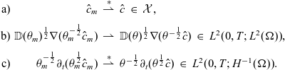 \begin{equation*}\begin{array}{rr@{\,\,}c@{\,\,}l}\text{a)} & \hat{c}_m & \stackrel{*}{\rightharpoonup} & \hat{c}\ \in\ \mathcal{X} ,\\ \\[-7pt]\text{b)} & \mathbb{D}(\theta_m)^{\frac{1}{2}}\nabla(\theta_m^{-\frac{1}{2}}\hat{c}_m) & \rightharpoonup & \mathbb{D}(\theta)^{\frac{1}{2}}\nabla(\theta^{-\frac{1}{2}}\hat{c})\ \in\ L^2(0,T;L^2(\Omega)) ,\\\\[-7pt] \text{c)} & \theta_m^{-\frac{1}{2}}\partial_t(\theta_m^{\frac{1}{2}}\hat{c}_m) & \stackrel{*}{\rightharpoonup} & \theta^{-\frac{1}{2}}\partial_t(\theta^{\frac{1}{2}}\hat{c})\ \in\ L^2(0,T;H^{-1}(\Omega)) .\end{array}\end{equation*}
Proof. Due to the estimates obtained in Theorem 3.5 and the isomorphism between the spaces $\mathcal{X}_\theta$
and
$\mathcal{X}_\theta$
and $\mathcal{X}$
, cf. Lemma 3,
$\mathcal{X}$
, cf. Lemma 3, $(\hat{c}_{\varepsilon})_{\varepsilon>0}$
is uniformly bounded in
$(\hat{c}_{\varepsilon})_{\varepsilon>0}$
is uniformly bounded in $\mathcal{X}$
with respect to
$\mathcal{X}$
with respect to $\varepsilon>0$
and hence there is a subsequence
$\varepsilon>0$
and hence there is a subsequence $(\hat{c}_m)_{m\in\mathbb{N}}$
converging weakly
$(\hat{c}_m)_{m\in\mathbb{N}}$
converging weakly $^*$
to a limit
$^*$
to a limit $\hat{c}\in\mathcal{X}$
. Then the Lemma of Aubin-Lions implies strong convergence of a subsequence of
$\hat{c}\in\mathcal{X}$
. Then the Lemma of Aubin-Lions implies strong convergence of a subsequence of $(\hat{c}_m)_{m\in\mathbb{N}}$
in
$(\hat{c}_m)_{m\in\mathbb{N}}$
in $C(0,T;L^2(\Omega))$
to
$C(0,T;L^2(\Omega))$
to $\hat{c}$
such that in particular
$\hat{c}$
such that in particular $\partial_t\hat{c}_m\stackrel{*}{\rightharpoonup}\partial_t\hat{c}$
with respect to
$\partial_t\hat{c}_m\stackrel{*}{\rightharpoonup}\partial_t\hat{c}$
with respect to $L^2(0,T;H^{-1}(\Omega))$
. These properties together with the weak convergence of
$L^2(0,T;H^{-1}(\Omega))$
. These properties together with the weak convergence of $(\theta_m^{-\frac{1}{2}}\partial_t\theta_m)_{m\in\mathbb{N}}$
lead to
$(\theta_m^{-\frac{1}{2}}\partial_t\theta_m)_{m\in\mathbb{N}}$
lead to
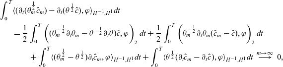 \begin{align*} \int_0^T & \langle(\partial_t(\theta_m^{\frac{1}{2}}\hat{c}_m) - \partial_t(\theta^{\frac{1}{2}}\hat{c}),\varphi\rangle_{H^{-1},H^1}dt \\ &= \frac{1}{2}\int_0^T\left((\theta_m^{-\frac{1}{2}}\partial_t\theta_m - \theta^{-\frac{1}{2}}\partial_t\theta)\hat{c},\varphi\right)_2dt+ \frac{1}{2}\int_0^T\left(\theta_m^{-\frac{1}{2}}\partial_t\theta_m(\hat{c}_m - \hat{c}),\varphi\right)_2dt \\ &\qquad +\int_0^T\langle(\theta_m^{\frac{1}{2}}-\theta^{\frac{1}{2}})\partial_t\hat{c}_m,\varphi\rangle_{H^{-1},H^1}dt+\int_0^T\langle\theta^{\frac{1}{2}}(\partial_t\hat{c}_m-\partial_t\hat{c}),\varphi\rangle_{H^{-1},H^1}dt\ \stackrel{m\to\infty}{\longrightarrow}\ 0 ,\end{align*}
implying weakly $^*$
convergence of
$^*$
convergence of $\partial_t(\theta_m^{\frac{1}{2}}\hat{c}_m)$
to
$\partial_t(\theta_m^{\frac{1}{2}}\hat{c}_m)$
to $\partial_t(\theta^{\frac{1}{2}}\hat{c})$
. This property allows us to identify the limit
$\partial_t(\theta^{\frac{1}{2}}\hat{c})$
. This property allows us to identify the limit $\xi$
of
$\xi$
of $\theta_m^{-\frac{1}{2}}\partial_t(\theta_m^{\frac{1}{2}} \hat{c}_m)$
in
$\theta_m^{-\frac{1}{2}}\partial_t(\theta_m^{\frac{1}{2}} \hat{c}_m)$
in $L^2(0,T;H^{-1}(\Omega))$
. Due to the strong
$L^2(0,T;H^{-1}(\Omega))$
. Due to the strong $L^\infty$
-convergence of
$L^\infty$
-convergence of $\theta_m^{\frac{1}{2}}$
to
$\theta_m^{\frac{1}{2}}$
to $\theta^{\frac{1}{2}}$
we have weak
$\theta^{\frac{1}{2}}$
we have weak $^*$
convergence of the product
$^*$
convergence of the product $\theta_m^{\frac{1}{2}} \cdot \theta_m^{-\frac{1}{2}}\partial_t(\theta_m^{\frac{1}{2}} \hat{c}_m)=\partial_t(\theta_m^{\frac{1}{2}} \hat{c}_m)$
to
$\theta_m^{\frac{1}{2}} \cdot \theta_m^{-\frac{1}{2}}\partial_t(\theta_m^{\frac{1}{2}} \hat{c}_m)=\partial_t(\theta_m^{\frac{1}{2}} \hat{c}_m)$
to $\theta^{\frac{1}{2}}\cdot \xi=\partial_t(\theta^{\frac{1}{2}} \hat{c})$
, i.e.
$\theta^{\frac{1}{2}}\cdot \xi=\partial_t(\theta^{\frac{1}{2}} \hat{c})$
, i.e. $\xi=\theta^{-\frac{1}{2}}\partial_t(\theta^{\frac{1}{2}}\hat{c})$
.
$\xi=\theta^{-\frac{1}{2}}\partial_t(\theta^{\frac{1}{2}}\hat{c})$
.
Similarly, we see that a subsequence of $\mathbb{D}(\theta_m)^{\frac{1}{2}}\nabla(\theta_m^{-\frac{1}{2}}\hat{c}_m)$
converges weakly to
$\mathbb{D}(\theta_m)^{\frac{1}{2}}\nabla(\theta_m^{-\frac{1}{2}}\hat{c}_m)$
converges weakly to $\mathbb{D}(\theta)^{\frac{1}{2}}\nabla(\theta^{-\frac{1}{2}}\hat{c})$
: The uniform boundedness ensures the existence of a limit
$\mathbb{D}(\theta)^{\frac{1}{2}}\nabla(\theta^{-\frac{1}{2}}\hat{c})$
: The uniform boundedness ensures the existence of a limit $\gamma\in L^2(0,T;L^2(\Omega))$
, cf. Section 3.2.4. On the other hand (3.15) implies with
$\gamma\in L^2(0,T;L^2(\Omega))$
, cf. Section 3.2.4. On the other hand (3.15) implies with $\mathbb{D}(\theta)=\theta$
the weak
$\mathbb{D}(\theta)=\theta$
the weak $L^2(\Omega_T)$
-convergence
$L^2(\Omega_T)$
-convergence
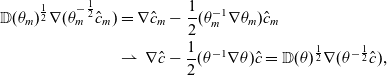 \begin{align*}\mathbb{D}(\theta_m)^{\frac{1}{2}}\nabla(\theta_m^{-\frac{1}{2}}\hat{c}_m) &= \nabla\hat{c}_m-\frac{1}{2}(\theta_m^{-1}\nabla\theta_m)\hat{c}_m\\&\rightharpoonup\ \nabla\hat{c}-\frac{1}{2}(\theta^{-1}\nabla\theta)\hat{c}=\mathbb{D}(\theta)^{\frac{1}{2}}\nabla(\theta^{-\frac{1}{2}}\hat{c}) ,\end{align*}
which allows to identify $\gamma$
.
$\gamma$
.
Since the energy estimate stated in Theorem 3.5 is uniform with respect to $\varepsilon>0$
, it is inherited to the limit
$\varepsilon>0$
, it is inherited to the limit $\hat{c}$
such that
$\hat{c}$
such that
 \begin{align*}\|\hat{c}\|^2_{L^\infty(L^2)} + \|\mathbb{D}(\theta)^{\frac{1}{2}}\nabla (\theta^{-\frac{1}{2}}\hat{c})\|^2_{L^2(L^2)} + \|\theta^{-\frac{1}{2}}\partial_t(\theta^{\frac{1}{2}} \hat{c})\|_{L^2(H^{-1})}^2 < \infty .\end{align*}
Remark 8 Due to Lemma 3 and Remark 7 these norms are equivalent to the corresponding norms of the standard function space $\mathcal{X}$
. Nevertheless, it is reasonable to represent the energy estimate with respect to these weighted norms since they arise naturally from the weak formulation (3.14). Furthermore, we remark that the energy estimate can be transformed to an energy estimate in the non-transformed physical concentration c. In particular, this concentration may be unbounded, but does not blow up worse than
$\mathcal{X}$
. Nevertheless, it is reasonable to represent the energy estimate with respect to these weighted norms since they arise naturally from the weak formulation (3.14). Furthermore, we remark that the energy estimate can be transformed to an energy estimate in the non-transformed physical concentration c. In particular, this concentration may be unbounded, but does not blow up worse than $\theta^{-\frac{1}{2}}$
.
$\theta^{-\frac{1}{2}}$
.
Theorem 3.6 (Existence transport problem)Under the Assumptions 1, 2, and 3, the condition $\hat{c}_0\in L^2(\Omega)$
and the additional smallness assumption (3.19) if
$\hat{c}_0\in L^2(\Omega)$
and the additional smallness assumption (3.19) if $k=3$
, the limit
$k=3$
, the limit $\hat{c}\in\mathcal{X}$
given in Lemma 4 satisfies the weak formulation of the degenerate problem (3.14).
$\hat{c}\in\mathcal{X}$
given in Lemma 4 satisfies the weak formulation of the degenerate problem (3.14).
Proof. We have for all test functions $\varphi\in L^2(0,T;H_0^1(\Omega))$
the following convergences:
$\varphi\in L^2(0,T;H_0^1(\Omega))$
the following convergences:
Evolution Term:
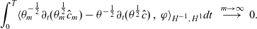 \begin{align*}\int_0^T\langle \theta_m^{-\frac{1}{2}}\partial_t(\theta_m^{\frac{1}{2}}\hat{c}_m)-\theta^{-\frac{1}{2}}\partial_t(\theta^{\frac{1}{2}}\hat{c})\,,\,\varphi\rangle_{H^{-1},\,H^1} dt\ \ \stackrel{m\to\infty}{\longrightarrow}\ 0 .\end{align*}
according to the corresponding weak- $^*$
convergence as stated in Lemma 4, c).
$^*$
convergence as stated in Lemma 4, c).
Reaction Term: The Lipschitz property (3.11) of $\hat{R}(\hat{c})$
leads to
$\hat{R}(\hat{c})$
leads to
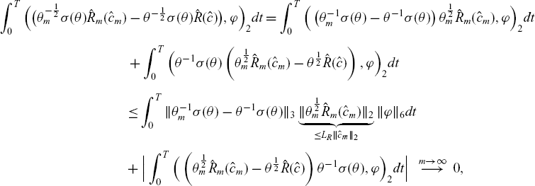 \begin{align*}\int_0^T\Big(\big(\theta_m^{-\frac{1}{2}}\sigma(\theta)\hat{R}_m(\hat{c}_m) &- \theta^{-\frac{1}{2}}\sigma(\theta)\hat{R}(\hat{c})\big),\varphi\Big)_2 dt=\int_0^T\Big(\left(\theta_m^{-1}\sigma(\theta)-\theta^{-1}\sigma(\theta)\right)\theta_m^{\frac{1}{2}}\hat{R}_m(\hat{c}_m),\varphi\Big)_2 dt\notag\\[4pt] & +\int_0^T\Big(\theta^{-1}\sigma(\theta)\left(\theta_m^{\frac{1}{2}}\hat{R}_m(\hat{c}_m)-\theta^{\frac{1}{2}}\hat{R}(\hat{c})\right),\varphi\Big)_2 dt\notag\\[3pt] & \leq \int_0^T\|\theta_m^{-1}\sigma(\theta)-\theta^{-1}\sigma(\theta)\|_{3}\underbrace{\|\theta_m^{\frac{1}{2}}\hat{R}_m(\hat{c}_m)\|_2}_{\leq L_R\|\hat{c}_m\|_2}\|\varphi\|_{6} dt\notag\\[3pt]& +\Big|\int_0^T\Big(\left(\theta_m^{\frac{1}{2}}\hat{R}_m(\hat{c}_m)-\theta^{\frac{1}{2}}\hat{R}(\hat{c})\right)\theta^{-1}\sigma(\theta),\varphi\Big)_2 dt\Big|\ \ \stackrel{m\to\infty}{\longrightarrow}\ 0 ,\notag\end{align*}
where the second summand on the right-hand side can be estimated with Assumption 2 and (3.11) as follows
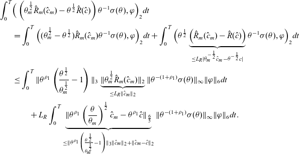 \begin{align*}\int_0^T & \Big(\left(\theta_m^{\frac{1}{2}}\hat{R}_m(\hat{c}_m)-\theta^{\frac{1}{2}}\hat{R}(\hat{c})\right)\theta^{-1}\sigma(\theta),\varphi\Big)_2 dt\\[2pt]&=\int_0^T\Big((\theta_m^{\frac{1}{2}}-\theta^{\frac{1}{2}})\hat{R}_m(\hat{c}_m)\theta^{-1}\sigma(\theta),\varphi\Big)_2 dt+ \int_0^T\Big(\theta^{\frac{1}{2}}\underbrace{\left(\hat{R}_m(\hat{c}_m)-\hat{R}(\hat{c})\right)}_{\leq L_R|\theta_m^{-\frac{1}{2}}\hat{c}_m-\theta^{-\frac{1}{2}}c|}\theta^{-1}\sigma(\theta),\varphi\Big)_2 dt\\[2pt]&\leq\int_0^T\|\theta^{\rho_1}\left(\frac{\theta^{\frac{1}{2}}}{\theta_m^{\frac{1}{2}}}-1\right)\|_3\underbrace{\|\theta_m^{\frac{1}{2}}\hat{R}_m(\hat{c}_m)\|_2}_{\leq L_R\|\hat{c}_m\|_2}\|\theta^{-(1+\rho_1)}\sigma(\theta)\|_{\infty}\|\varphi\|_6 dt\\[2pt]&\qquad+L_R\int_0^T\underbrace{\|\theta^{\rho_1}\left(\frac{\theta}{\theta_m}\right)^\frac{1}{2}\hat{c}_m-\theta^{\rho_1}\hat{c}\|_{\frac{6}{5}}}_{\leq \|\theta^{\rho_1}\left(\frac{\theta^{\frac{1}{2}}}{\theta_m^{\frac{1}{2}}}-1\right)\|_3\|\hat{c}_m\|_2+\|\hat{c}_m-\hat{c}\|_2}\|\theta^{-(1+\rho_1)}\sigma(\theta)\|_{\infty}\|\varphi\|_6 dt .\end{align*}
Let us define for $m\in\mathbb{N}$
and
$m\in\mathbb{N}$
and $t\in(0,T)$
the subdomain
$t\in(0,T)$
the subdomain $\Omega_m(t):=\{x\in\Omega:\theta(x,t)\geq \varepsilon_m\}$
, where
$\Omega_m(t):=\{x\in\Omega:\theta(x,t)\geq \varepsilon_m\}$
, where $\varepsilon_m>0$
corresponds to
$\varepsilon_m>0$
corresponds to $\theta_m$
via (3.17), i.e.
$\theta_m$
via (3.17), i.e. $\theta_m\geq\varepsilon_m$
and
$\theta_m\geq\varepsilon_m$
and $\theta_m=\theta$
for all
$\theta_m=\theta$
for all $x\in\Omega_m(t)$
. Moreover, there holds
$x\in\Omega_m(t)$
. Moreover, there holds $\lim_{m\to\infty}\varepsilon_m=0$
. Consequently, the right-hand side of the above estimate converges since
$\lim_{m\to\infty}\varepsilon_m=0$
. Consequently, the right-hand side of the above estimate converges since $\left(\frac{\theta}{\theta_m}\right)^{\frac{1}{2}}=1$
in
$\left(\frac{\theta}{\theta_m}\right)^{\frac{1}{2}}=1$
in $\Omega_m(t)$
and hence
$\Omega_m(t)$
and hence
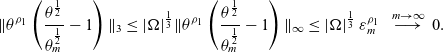 \begin{equation} \|\theta^{\rho_1}\left(\frac{\theta^{\frac{1}{2}}}{\theta_m^{\frac{1}{2}}}-1\right)\|_3\leq |\Omega|^{\frac{1}{3}}\|\theta^{\rho_1}\left(\frac{\theta^{\frac{1}{2}}}{\theta_m^{\frac{1}{2}}}-1\right)\|_\infty \leq|\Omega|^{\frac{1}{3}}\,\varepsilon_m^{\rho_1}\ \ \stackrel{m\to\infty}{\longrightarrow}\ 0 .\end{equation}
Similarly, the first summand on the right-hand side of (3.26) can be estimated by applying (3.27) and Assumption 2.
Diffusive Term: Applying the weak convergence as stated in Lemma 4, b), it holds
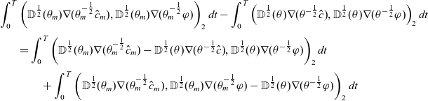 \begin{align*}\int_0^T & \left(\mathbb{D}^{\frac{1}{2}}(\theta_m)\nabla (\theta_m^{-\frac{1}{2}}\hat{c}_m),\mathbb{D}^{\frac{1}{2}}(\theta_m)\nabla(\theta_m^{-\frac{1}{2}}\varphi)\right)_2 dt-\int_0^T\left({\mathbb{D}^{\frac{1}{2}}(\theta)\nabla (\theta^{-\frac{1}{2}}\hat{c})},\mathbb{D}^{\frac{1}{2}}(\theta)\nabla(\theta^{-\frac{1}{2}}\varphi)\right)_2 dt\\[2pt]&= \int_0^T\left(\mathbb{D}^{\frac{1}{2}}(\theta_m)\nabla (\theta_m^{-\frac{1}{2}}\hat{c}_m)-{\mathbb{D}^{\frac{1}{2}}(\theta)\nabla (\theta^{-\frac{1}{2}}\hat{c})},\mathbb{D}^{\frac{1}{2}}(\theta)\nabla(\theta^{-\frac{1}{2}}\varphi)\right)_2 dt \\[2pt] &\qquad + \int_0^T\left(\mathbb{D}^{\frac{1}{2}}(\theta_m)\nabla (\theta_m^{-\frac{1}{2}}\hat{c}_m),\mathbb{D}^{\frac{1}{2}}(\theta_m)\nabla(\theta_m^{-\frac{1}{2}}\varphi)-\mathbb{D}^{\frac{1}{2}}(\theta)\nabla(\theta^{-\frac{1}{2}}\varphi)\right)_2 dt\end{align*}
for all $\varphi\in L^2(0,T;H_0^1(\Omega))$
, where the first summand on the right-hand side vanishes. Due to
$\varphi\in L^2(0,T;H_0^1(\Omega))$
, where the first summand on the right-hand side vanishes. Due to $\mathbb{D}(\theta)=\theta$
, cf. Assumption 1, and the uniform estimate stated in Theorem 3.3, the second summand on the right-hand side can be estimated by
$\mathbb{D}(\theta)=\theta$
, cf. Assumption 1, and the uniform estimate stated in Theorem 3.3, the second summand on the right-hand side can be estimated by
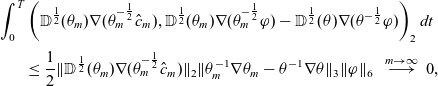 \begin{align*}\int_0^T & \left(\mathbb{D}^{\frac{1}{2}}(\theta_m)\nabla (\theta_m^{-\frac{1}{2}}\hat{c}_m),\mathbb{D}^{\frac{1}{2}}(\theta_m)\nabla(\theta_m^{-\frac{1}{2}}\varphi)-\mathbb{D}^{\frac{1}{2}}(\theta)\nabla(\theta^{-\frac{1}{2}}\varphi)\right)_2 dt\\[2pt]&\leq \frac{1}{2}\|\mathbb{D}^{\frac{1}{2}}(\theta_m)\nabla (\theta_m^{-\frac{1}{2}}\hat{c}_m)\|_2 \|\theta_m^{-1}\nabla\theta_m-\theta^{-1}\nabla\theta\|_3\|\varphi\|_6 \ \ \stackrel{m\to\infty}{\longrightarrow}\ 0 ,\end{align*}
where the sequence $(\theta_m^{-1}\nabla\theta_m)_{m\in\mathbb{N}}$
even converges in a strong sense since the corresponding
$(\theta_m^{-1}\nabla\theta_m)_{m\in\mathbb{N}}$
even converges in a strong sense since the corresponding $L^3$
-norms converge to
$L^3$
-norms converge to $\|\theta^{-1}\nabla\theta\|_3$
.
$\|\theta^{-1}\nabla\theta\|_3$
.
Advective and stabilisation term: Since $\mathbb{D}(\theta)=\theta$
and
$\mathbb{D}(\theta)=\theta$
and $k\geq 3$
, cf. Assumption 1, and applying (3.7b), we obtain
$k\geq 3$
, cf. Assumption 1, and applying (3.7b), we obtain
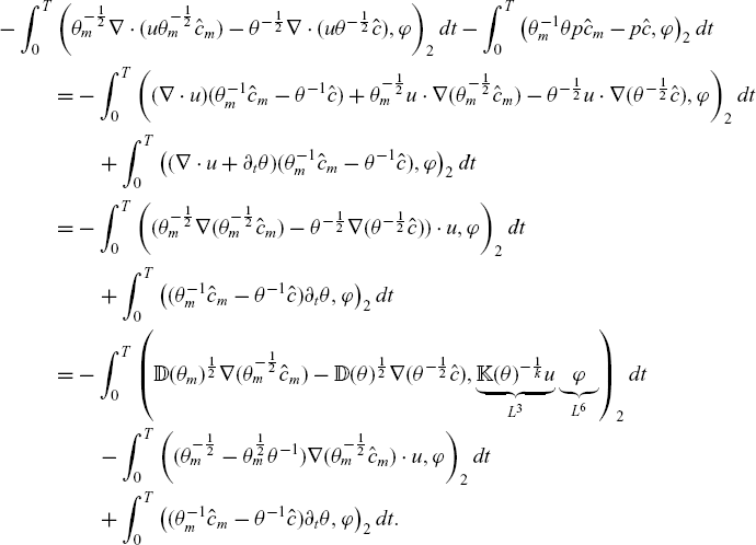 \begin{align}-\int_0^T & \left(\theta_m^{-\frac{1}{2}}\nabla\cdot(u\theta_m^{-\frac{1}{2}}\hat{c}_m)-\theta^{-\frac{1}{2}}\nabla\cdot(u\theta^{-\frac{1}{2}}\hat{c}),\varphi\right)_2 dt-\int_0^T\left(\theta_m^{-1}\theta p\hat{c}_m-p\hat{c},\varphi\right)_2 dt \notag\\[2pt]&= -\int_0^T\left((\nabla\cdot u)(\theta_m^{-1}\hat{c}_{m}-\theta^{-1}\hat{c})+\theta_{m}^{-\frac{1}{2}}u\cdot\nabla(\theta_m^{-\frac{1}{2}}\hat{c}_m)-\theta^{-\frac{1}{2}}u\cdot\nabla(\theta^{-\frac{1}{2}}\hat{c}),\varphi\right)_2 dt \notag\\[2pt]&\qquad +\int_0^T\left((\nabla\cdot u+\partial_t\theta)(\theta_m^{-1}\hat{c}_{m}-\theta^{-1}\hat{c}),\varphi\right)_2 dt \notag\\[2pt]&= -\int_0^T\left((\theta_{m}^{-\frac{1}{2}}\nabla(\theta_m^{-\frac{1}{2}}\hat{c}_m)-\theta^{-\frac{1}{2}}\nabla(\theta^{-\frac{1}{2}}\hat{c}))\cdot u,\varphi\right)_2 dt \notag\\[2pt]&\qquad +\int_0^T\left((\theta_m^{-1}\hat{c}_{m}-\theta^{-1}\hat{c})\partial_t\theta,\varphi\right)_2 dt \notag\\&= -\int_0^T\left(\mathbb{D}(\theta_m)^{\frac{1}{2}}\nabla(\theta_m^{-\frac{1}{2}}\hat{c}_m)-\mathbb{D}(\theta)^{\frac{1}{2}}\nabla(\theta^{-\frac{1}{2}}\hat{c}),\underbrace{\mathbb{K}(\theta)^{-\frac{1}{k}}u}_{L^3}\underbrace{\varphi}_{L^6}\right)_2 dt \notag\\ &\qquad - \int_0^T\left((\theta_m^{-\frac{1}{2}}-\theta_m^{\frac{1}{2}}\theta^{-1})\nabla(\theta_m^{-\frac{1}{2}}\hat{c}_m)\cdot u,\varphi\right)_2 dt\notag\\&\qquad +\int_0^T\left((\theta_m^{-1}\hat{c}_{m}-\theta^{-1}\hat{c})\partial_t\theta,\varphi\right)_2 dt . \end{align}
Again Lemma 4, b) implies the convergence of the first summand on the right-hand side. If $k>3$
, the second summand can similarly to (3.27) be estimated by
$k>3$
, the second summand can similarly to (3.27) be estimated by
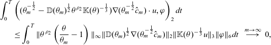 \begin{align*}\int_0^T & \left((\theta_m^{-\frac{1}{2}}-\mathbb{D}(\theta_m)^{\frac{1}{2}}\theta^{\rho_2}\mathbb{K}(\theta)^{-\frac{1}{3}})\nabla(\theta_m^{-\frac{1}{2}}\hat{c}_m)\cdot u,\varphi\right)_2 dt\\&\leq\int_0^T\|\theta^{\rho_2}\left(\frac{\theta}{\theta_m}-1\right)\|_\infty\|\mathbb{D}(\theta_m)^{\frac{1}{2}}\nabla(\theta_m^{-\frac{1}{2}}\hat{c}_m)\|_2\|\mathbb{K}(\theta)^{-\frac{1}{3}}u\|_3\|\varphi\|_6 dt\ \ \stackrel{m\to\infty}{\longrightarrow}\ 0,\end{align*}
with $\rho_2:=\frac{k}{3}-1>0$
.
$\rho_2:=\frac{k}{3}-1>0$
.
Contrarily, for the case $k=3$
, the following density argument is needed. First we consider
$k=3$
, the following density argument is needed. First we consider
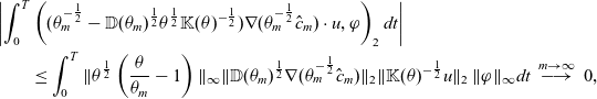 \begin{align*}&\left|\int_0^T \left((\theta_m^{-\frac{1}{2}}-\mathbb{D}(\theta_m)^{\frac{1}{2}}\theta^{\frac{1}{2}}\mathbb{K}(\theta)^{-\frac{1}{2}})\nabla(\theta_m^{-\frac{1}{2}}\hat{c}_m)\cdot u,\varphi\right)_2 dt\right|\\&\qquad \leq \int_0^T\|\theta^{\frac{1}{2}}\left(\frac{\theta}{\theta_m}-1\right)\|_\infty\|\mathbb{D}(\theta_m)^{\frac{1}{2}}\nabla(\theta_m^{-\frac{1}{2}}\hat{c}_m)\|_2\|\mathbb{K}(\theta)^{-\frac{1}{2}}u\|_2\,\|\varphi\|_\infty dt\ \stackrel{m\to\infty}{\longrightarrow}\ 0,\end{align*}
for all smooth test functions $\varphi\in C_0^\infty(\Omega_T)$
. The density of
$\varphi\in C_0^\infty(\Omega_T)$
. The density of $C_0^\infty(\Omega_T)$
in
$C_0^\infty(\Omega_T)$
in $L^2(0,T;L^6(\Omega))$
leads for an arbitrary test function
$L^2(0,T;L^6(\Omega))$
leads for an arbitrary test function $\varphi\in L^2(0,T;L^6(\Omega))$
and a sequence of smooth functions
$\varphi\in L^2(0,T;L^6(\Omega))$
and a sequence of smooth functions $\varphi_\ell\in C_0^\infty(\Omega_T)$
converging to
$\varphi_\ell\in C_0^\infty(\Omega_T)$
converging to $\varphi$
as
$\varphi$
as $\ell\to\infty$
to the following result. Let
$\ell\to\infty$
to the following result. Let $\delta>0$
. Since
$\delta>0$
. Since $\|\mathbb{D}(\theta_m)^{\frac{1}{2}}\nabla\cdot(\theta_m^{-\frac{1}{2}}\hat{c}_m)\|_{L^2(L^2)}$
is uniformly bounded, choosing
$\|\mathbb{D}(\theta_m)^{\frac{1}{2}}\nabla\cdot(\theta_m^{-\frac{1}{2}}\hat{c}_m)\|_{L^2(L^2)}$
is uniformly bounded, choosing $\ell$
sufficiently large such that
$\ell$
sufficiently large such that
 \begin{equation*}\sup_{t\in(0,T)}\left(\|\frac{\theta(t)}{\theta_m(t)}-1\|_\infty\|\mathbb{K}(\theta)^{-\frac{1}{3}}u(t)\|_3\right)\|\mathbb{D}(\theta_m)^{\frac{1}{2}}\nabla(\theta_m^{-\frac{1}{2}}\hat{c}_m)\|_{L^2(L^2)}\|\varphi-\varphi_\ell\|_{L^2(L^6)}<\frac{\delta}{2},\end{equation*}
and afterwards choosing m in such a way that
 \begin{equation*}\sup_{t\in(0,T)}\left(\|\theta^{\frac{1}{2}}(t)\left(\frac{\theta(t)}{\theta_m(t)}-1\right)\|_\infty\|\mathbb{K}(\theta)^{-\frac{1}{2}}u(t)\|_2\right)\|\mathbb{D}(\theta_m)^{\frac{1}{2}}\nabla(\theta_m^{-\frac{1}{2}}\hat{c}_m)\|_{L^2(L^2)}\|\varphi_\ell\|_{L^2(L^\infty)}<\frac{\delta}{2},\end{equation*}
actually leads for $\varphi\in L^2(0,T;L^6(\Omega))$
to
$\varphi\in L^2(0,T;L^6(\Omega))$
to
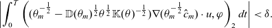 \begin{equation*}\left|\int_0^T \left((\theta_m^{-\frac{1}{2}}-\mathbb{D}(\theta_m)^{\frac{1}{2}}\theta^{\frac{1}{2}}\mathbb{K}(\theta)^{-\frac{1}{2}})\nabla(\theta_m^{-\frac{1}{2}}\hat{c}_m)\cdot u,\varphi\right)_2 dt\right|<\delta .\end{equation*}
Finally, applying Assumption 3, d) and the weak* convergence of $\frac{\theta}{\theta_m}$
to 1 in
$\frac{\theta}{\theta_m}$
to 1 in $L^\infty(\Omega)$
to the last term on the right-hand side of (3.28) yields
$L^\infty(\Omega)$
to the last term on the right-hand side of (3.28) yields
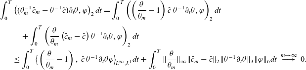 \begin{align*} \int_0^T & \left((\theta_m^{-1}\hat{c}_{m}-\theta^{-1}\hat{c})\partial_t\theta,\varphi\right)_2dt= \int_0^T\left(\left(\frac{\theta}{\theta_m}-1\right)\hat{c}\,\theta^{-1}\partial_t\theta,\varphi\right)_2dt\\[3pt] &\quad + \int_0^T\left(\frac{\theta}{\theta_m}\left(\hat{c}_{m}-\hat{c}\right)\theta^{-1}\partial_t\theta,\varphi\right)_2dt\\&\leq \int_0^T\big\langle\left(\frac{\theta}{\theta_m}-1\right),\,\hat{c}\,\theta^{-1}\partial_t\theta\varphi\big\rangle_{L^\infty,L^1}dt+ \int_0^T\|\frac{\theta}{\theta_m}\|_\infty\|\hat{c}_{m}-\hat{c}\|_2\|\theta^{-1}\partial_t\theta\|_3\|\varphi\|_6 dt\ \stackrel{m\to\infty}{\longrightarrow}\ 0 .\\[-30pt]\end{align*}
3.2.6 Existence and uniqueness
Combining the results of the previous sections, we obtain weak solvability of the original degenerating model. However, the transport equation (2.2) is lost within the area with $\theta=0$
since it trivializes to
$\theta=0$
since it trivializes to $0=0$
. In such a situation of vanishing porosity, the behavior of c is not clearly defined and hence a uniqueness assertion needs to be restricted to the subdomain
$0=0$
. In such a situation of vanishing porosity, the behavior of c is not clearly defined and hence a uniqueness assertion needs to be restricted to the subdomain $\Omega_0:=\{(x,t)\in\Omega_T|\theta(x,t)\neq0\}$
.
$\Omega_0:=\{(x,t)\in\Omega_T|\theta(x,t)\neq0\}$
.
Theorem 3.7 (Coupled degenerating problem)Under Assumptions 1, 2, and 3, the condition $\hat{c}_0\in L^2(\Omega)$
, and the additional smallness assumption (3.19) if
$\hat{c}_0\in L^2(\Omega)$
, and the additional smallness assumption (3.19) if $k=3$
, there exists a weaksolution
$k=3$
, there exists a weaksolution
 \begin{equation*}(\hat{c},\hat{u},\hat{p})\in \mathcal{X}\times L^\infty(0,T;H_{\theta,div,0}(\Omega))\times L^\infty(0,T;L^2(\Omega)),\end{equation*}
to the degenerating transformed problems (3.2) and (3.19) corresponding to the coupled Model 1 and 2. Moreover, this solution is unique and $\hat{c}$
satisfies non-negativity on
$\hat{c}$
satisfies non-negativity on $\Omega_0$
.
$\Omega_0$
.
Proof. The Theorems 3.2 and 3.6 directly ensure the existence of a weak solution $(\hat{c},\hat{u},\hat{p})$
to (3.2) and (3.10). The uniqueness of this solution in
$(\hat{c},\hat{u},\hat{p})$
to (3.2) and (3.10). The uniqueness of this solution in $\Omega_0$
is verified by a straightforward argument (for the sake of readability it is expressed in the physical non-transformed values): Let
$\Omega_0$
is verified by a straightforward argument (for the sake of readability it is expressed in the physical non-transformed values): Let $(c_i,u_i,p_i)$
,
$(c_i,u_i,p_i)$
, $i=1,2$
, two weak solutions of (2.1) – (2.2). Then
$i=1,2$
, two weak solutions of (2.1) – (2.2). Then $\tilde{u}:=u_1-u_2$
and
$\tilde{u}:=u_1-u_2$
and $\tilde{p}:=p_1-p_2$
fulfill the equations
$\tilde{p}:=p_1-p_2$
fulfill the equations
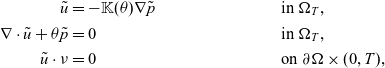 \begin{align*} \tilde{u} &= -\mathbb{K}(\theta)\nabla \tilde{p} && \text{in }\Omega_T ,\\ \nabla\cdot \tilde{u} + \theta \tilde{p} &= 0 && \text{in }\Omega_T ,\notag\\ \tilde{u}\cdot \nu &= 0 && \text{on } \partial\Omega\times (0,T),\end{align*}
with the unique solution $\tilde{u}=0$
and
$\tilde{u}=0$
and $\tilde{p}=0$
, cf. [Reference Arbogast and Taicher3]. Furthermore, the function
$\tilde{p}=0$
, cf. [Reference Arbogast and Taicher3]. Furthermore, the function $\tilde{c}:=c_1-c_2$
satisfies the transport equation
$\tilde{c}:=c_1-c_2$
satisfies the transport equation
 \begin{align*} \partial_t(\theta \tilde{c}) - \nabla\cdot\mathbb{D}(\theta)\nabla \tilde{c} &= -\sigma(\theta)(R(c_1)-R(c_2)) && \text{in }\Omega_T,\end{align*}
with zero initial and boundary conditions. Testing with $\tilde{c}$
leads to
$\tilde{c}$
leads to
 \begin{align*}\frac{1}{2}\|\theta^{\frac{1}{2}}\tilde{c}(t)\|_2^2+\int_0^t\|\mathbb{D}(\theta)^{\frac{1}{2}}\nabla \tilde{c}\|_2^2 ds\leq\int_0^t\|\sigma(\theta)\|_\infty\|R(c_1)-R(c_2)\|_2\|\tilde{c}\|_2 ds+ \frac{1}{2}\int_0^t\|\partial_t\theta\|_\infty\|\tilde{c}\|_2^2 ds .\end{align*}
Finally, the Lipschitz condition of R, cf. Assumption 2 and Gronwall’s Lemma yield
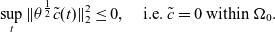 \begin{equation*}\sup_t\|\theta^{\frac{1}{2}}\tilde{c}(t)\|_2^2\leq0 ,\quad\text{i.e. }\tilde{c}=0\text{ within }\Omega_0 .\end{equation*}
The non-negativity follows along the same lines as the energy estimate testing the weak formulation with the negative part $c_-$
of the concentration. Thereby the reaction term is estimated via
$c_-$
of the concentration. Thereby the reaction term is estimated via
 \begin{align*} \int_\Omega \sigma(\theta)R(c)c_-dx \leq C_R\|\sigma(\theta)\|_\infty \|c_-\|_2^2,\end{align*}
according to Assumption 2. Again Gronwall’s Lemma guarantees the non-negativity on $\Omega_0$
.
$\Omega_0$
.
4 Discussion
In this research, we investigated a degenerating system of partial differential equations describing reactive flow and transport in altering porous media. For a prescribed, but vanishing porosity field, we proved the existence and uniqueness of non-negative weak solutions in porosity-weighted function spaces. We furthermore specified the conditions, under which these function spaces can be identified with standard Sobolev spaces.
Since the assumptions placed on the porosity and (scalar-valued) coefficients are in line with findings from the literature, our results apply to realistic scenarios. However, further research is needed to consider the fully coupled system, in which the porosity is an additional unknown being described by an ordinary differential equation or in an even more general setting by a level set function. In the latter setting and relying on the results from upscaling theory, anisotropic coefficients in their full tensorial form could also be taken into account.
Finally, a numerical realisation of scenarios with vanishing porosity and a related thorough numerical analysis as presented in [Reference Arbogast and Taicher3, Reference Arbogast and Taicher4] for the situation of a degenerate flow problem are of interest. First results in this direction for the coupled flow and transport problem are foundin [Reference Zech, Schulz and Ray30].
Acknowledgements
We thank Todd Arbogast, The University of Texas at Austin, Department of Mathematics, 2515 Speedway, StopC1200, Austin, Texas 78712-1202, USA for helpful discussions and advise. Moreover, we thank the reviewers for their advise, which improved the manuscript.
N. Ray was supported by the DFG Research Training Group 2339 Interfaces, Complex Structures and Singular Limits and the DFG Research Unit 2179 MadSoil.
