


1. Introduction
The narrow capture problem, as described here, concerns the average time required for a particle undergoing Brownian motion to encounter a region within the domain, referred to as a trap, which causes its motion to cease. It is mathematically defined as a Neumann–Dirichlet Poisson problem:
 \begin{equation} \begin{split}& \Delta u = -\dfrac{1}{D} \ , \quad x \in \Omega_0 \ ; \qquad \Omega_0 = \Omega \setminus \mathop{\cup}_{j = 1}^{N} \Omega_{\varepsilon_j} \ ; \\& \partial_n u = 0 \ , \quad x \in \partial\Omega \ ; \qquad u = 0 \ , \quad x \in \partial\Omega_{\varepsilon_j} \ , \quad j = 1, \ldots , N, \ \end{split}\end{equation}
where $\Omega\subset \mathbb{R}^n$
,
$\Omega\subset \mathbb{R}^n$
, $n=2,3$
, denotes the physical domain of the problem;
$n=2,3$
, denotes the physical domain of the problem; $\{\Omega_{\varepsilon_j}\}_{j = 1}^{N}$
are small trap domains within
$\{\Omega_{\varepsilon_j}\}_{j = 1}^{N}$
are small trap domains within $\Omega$
,
$\Omega$
, $\Omega_0$
is the domain except the traps, where the motion of particles takes place, and
$\Omega_0$
is the domain except the traps, where the motion of particles takes place, and $\partial_n$
is the normal derivative on the domain boundary
$\partial_n$
is the normal derivative on the domain boundary $\partial\Omega$
. The diffusivity D of the medium filling
$\partial\Omega$
. The diffusivity D of the medium filling $\Omega_0$
is assumed constant. The problem (1.1) describes the distribution of the mean capture time, the time u(x) needed for a particle to be captured by any trap, averaged over a large number of launches from the same point
$\Omega_0$
is assumed constant. The problem (1.1) describes the distribution of the mean capture time, the time u(x) needed for a particle to be captured by any trap, averaged over a large number of launches from the same point $x\in \Omega_0$
. An illustration of the problem is provided in Figure 1.
$x\in \Omega_0$
. An illustration of the problem is provided in Figure 1.

Figure 1. (a) A two-dimensional narrow capture problem in the unit disc containing internal traps with absorbing boundaries $\{\partial\Omega_{\epsilon_j}\}$
. (b) A three-dimensional narrow capture problem, a sample Brownian particle trajectory, leading to a capture in a trap (lowermost) denoted by purple colour.
$\{\partial\Omega_{\epsilon_j}\}$
. (b) A three-dimensional narrow capture problem, a sample Brownian particle trajectory, leading to a capture in a trap (lowermost) denoted by purple colour.
The boundary conditions on $\partial \Omega$
are reflective:
$\partial \Omega$
are reflective: $\partial_n u = 0$
, whereas the traps
$\partial_n u = 0$
, whereas the traps $\Omega_{\varepsilon_j}$
are characterised by immediate absorption of a Brownian particle, which is manifested by a Dirichlet boundary conditions
$\Omega_{\varepsilon_j}$
are characterised by immediate absorption of a Brownian particle, which is manifested by a Dirichlet boundary conditions $u = 0$
on all
$u = 0$
on all $\partial\Omega_{\varepsilon_j}$
.
$\partial\Omega_{\varepsilon_j}$
.
The above generic problem (1.1) affords a variety of physical interpretations, ranging from biological to electrostatic (see, e.g., [Reference Holcman and Schuss9, Reference Redner20] for an overview of applications). In this work, it will be strictly considered in terms of a particle undergoing Brownian motion [Reference Saffman and Delbrück23]. In this case, the problem regards the stopping time [Reference Metzler, Redner and Oshanin19, Reference Redner20] of a Brownian particle. When the path of the particle intersects the boundary of one of the traps, the particle is captured. This capture time may be interpreted as the time required for the particle to leave the confining domain; thus, it is often referred to as the first passage time [Reference Bressloff, Earnshaw and Ward1, Reference Bressloff and Newby2, Reference Holcman and Schuss10]. As Brownian motion is an inherently random process, the mean first passage time (MFPT) is considered. Interpreting the problem (1.1) accordingly, u is the MFPT; D is the diffusion coefficient, representing the mobility of the Brownian particle; $\Omega_{\varepsilon_j}$
is the portion of the domain occupied by the
$\Omega_{\varepsilon_j}$
is the portion of the domain occupied by the $j_{th}$
trap.
$j_{th}$
trap.
Given the physical domain and the number and sizes of the traps, it is of interest to ask whether there is an optimal arrangement of N traps within the domain which minimises the MFPT, or in other words, maximises the rate at which Brownian particles encounter the absorbing traps. Related work dedicated to similar optimisation, in the case that the traps are asymptotically small relative to the size of the domain, for various kinds of confining domains with interior or boundary traps, can be found, for example, in [Reference Cheviakov and Ward3, Reference Gilbert and Cheviakov7, Reference Iyaniwura, Wong, Macdonald and Ward12, Reference Kolokolnikov, Titcombe and Ward14, Reference Ridgway and Cheviakov21] and references therein. Both putative globally optimal and multiple locally optimal arrangements of boundary and volume traps have been computed in various settings. An important aspect of such computations is the existence of a large number of locally optimal particle arrangements with very close merit function values. This number quickly grows with N, increasing the computational difficulty of the determination of the globally optimal configuration; see, for example, [Reference Ridgway and Cheviakov21] where locally optimal configurations were systematically computed for particles located on the unit sphere, and the number of local minima exhibits exponential growth as N increases.
In the current contribution, we consider the narrow capture problem for the case of a 2D elliptical domain, elaborating on previous work on the subject for the case of a circular domain [Reference Kolokolnikov, Titcombe and Ward14], and the more general case of the elliptical domain [Reference Iyaniwura, Wong, Macdonald and Ward12], and examine specifically the case where traps are not of equal size. The paper is organised as follows. In Section 2, we briefly summarise results this work is based on. This includes the approximate asymptotic MFPT formulas that hold in the case that the traps are small relative to the domain size and are well separated, as well as the choice of merit function for average MFPT (AMFPT) optimisation.
Section 3 describes the optimisation method chosen in the current study, the algorithms, the details of their use, and some decisions made to facilitate comparison to previous studies. Specifically, we seek the optimal configuration of traps for numbers of traps $N \leq 50$
, and elliptic domains of sample eccentricities 0,
$N \leq 50$
, and elliptic domains of sample eccentricities 0, $0.472$
,
$0.472$
, $0.802$
, and
$0.802$
, and $0.995$
. In Section 4, the results of the study for N identical traps are presented. These results include the optimised values of the merit functions (related to the domain-average Brownian particle capture time) for each number of traps, and each domain eccentricity; in the case of the unit disc, the new computations are compared to those of the previous study [Reference Kolokolnikov, Titcombe and Ward14]. Distributions of traps for some illustrative cases are shown, and bulk measures of trap distribution including the closest-neighbour pairwise distance, smallest distance to the boundary, and area per trap are calculated for each of the optimised configurations of identical traps. It is also shown that unlike the cases of the disc- and sphere-shaped domains, where traps tend to be distributed about circular rings or spherical shells, respectively [Reference Gilbert and Cheviakov7, Reference Kolokolnikov, Titcombe and Ward14], optimal trap locations within an ellipse are generally not distributed about scaled versions of the domain boundary. While this often seems to be the case, we observed remarkable deviations from this trend, the most dramatic of which can be seen in Figure 10.
$0.995$
. In Section 4, the results of the study for N identical traps are presented. These results include the optimised values of the merit functions (related to the domain-average Brownian particle capture time) for each number of traps, and each domain eccentricity; in the case of the unit disc, the new computations are compared to those of the previous study [Reference Kolokolnikov, Titcombe and Ward14]. Distributions of traps for some illustrative cases are shown, and bulk measures of trap distribution including the closest-neighbour pairwise distance, smallest distance to the boundary, and area per trap are calculated for each of the optimised configurations of identical traps. It is also shown that unlike the cases of the disc- and sphere-shaped domains, where traps tend to be distributed about circular rings or spherical shells, respectively [Reference Gilbert and Cheviakov7, Reference Kolokolnikov, Titcombe and Ward14], optimal trap locations within an ellipse are generally not distributed about scaled versions of the domain boundary. While this often seems to be the case, we observed remarkable deviations from this trend, the most dramatic of which can be seen in Figure 10.
Section 5 is concerned with a more general case of unequal traps in an elliptic domain. Asymptotic formulas for the AMFPT are derived for this case, generalising those for the case of identical traps. Sample putative optimal configurations for traps of two kinds, for different trap size relations and domain eccentricities, are computed.
Section 6 contains a discussion of the results and some related problems.
2. Asymptotic MFPT for the elliptic domain with N identical traps
The main goal of this contribution is to further explore optimal configurations of absorbing traps found using asymptotic expansions for the circular and elliptical domains for which asymptotic MFPT formulae depending on trap positions are now available [Reference Iyaniwura, Wong, Macdonald and Ward12, Reference Kolokolnikov, Titcombe and Ward14]. To this end, numerical methods will be used to approximate the optimum configurations of larger numbers of traps than have previously been considered. In the case of the unit disc, the parameter space used in this study is general and does not assume any simplifying restrictions that have been imposed in previous works to reduce computational complexity. To begin, we recall the formulas for identical traps [Reference Iyaniwura, Wong, Macdonald and Ward12], following which, in Section 5, we derive the corresponding formulas for traps of differing sizes.
In essence, the problem at hand is to find the trap positions which minimise the spatial average of the MFPT u(x) in the elliptic domain $\Omega$
of area
$\Omega$
of area $|\Omega|$
, denoted by:
$|\Omega|$
, denoted by:
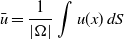 \begin{equation*}\bar{u}=\dfrac{1}{|\Omega|}\int u(x)\,dS\end{equation*}
and approximated by $\overline{u}_0$
in the leading order in terms of the deviation
$\overline{u}_0$
in the leading order in terms of the deviation $\sigma$
of the domain from the unit disc [Reference Iyaniwura, Wong, Macdonald and Ward12]. We now summarise the equations used to minimise
$\sigma$
of the domain from the unit disc [Reference Iyaniwura, Wong, Macdonald and Ward12]. We now summarise the equations used to minimise $\overline{u}_0$
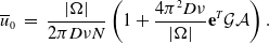
, as derived in [Reference Iyaniwura, Wong, Macdonald and Ward12, Reference Kolokolnikov, Titcombe and Ward14]. The unit disc will be considered a special case of the elliptical domain with zero eccentricity. In either case, when the domain contains N identical circular traps, each of radius
$\overline{u}_0$
, as derived in [Reference Iyaniwura, Wong, Macdonald and Ward12, Reference Kolokolnikov, Titcombe and Ward14]. The unit disc will be considered a special case of the elliptical domain with zero eccentricity. In either case, when the domain contains N identical circular traps, each of radius $\varepsilon$
, the approximate AMFPT satisfies [Reference Iyaniwura, Wong, Macdonald and Ward12]
$\varepsilon$
, the approximate AMFPT satisfies [Reference Iyaniwura, Wong, Macdonald and Ward12]
 \begin{equation} \overline{u}_0 \ = \ \dfrac{|\Omega|}{2\pi D\nu N} \ + \ \dfrac{2\pi}{N}\textbf{e}^{T}\mathcal{G} \mathcal{A},\end{equation}
where the column vector $\mathcal{A}$
satisfies
$\mathcal{A}$
satisfies
 \begin{equation} \sum_{j=1}^{N} \mathcal{A}_j = \dfrac{|\Omega|}{2\pi D}\end{equation}
and is given by the solution of the linear system:
 \begin{equation} \left[ I + 2\pi\!\nu\!\left( I - E \right)\mathcal{G} \right]\mathcal{A} \ = \ \dfrac{|\Omega|}{2\pi D N}\textbf{e}.\end{equation}
Here, $E \equiv \textbf{e}\textbf{e}^{T}/N$
,
$E \equiv \textbf{e}\textbf{e}^{T}/N$
, $\textbf{e} = (1, \ldots, 1)^{T}$
,
$\textbf{e} = (1, \ldots, 1)^{T}$
, $\nu \equiv -1/\log\varepsilon$
, and the Green’s matrix
$\nu \equiv -1/\log\varepsilon$
, and the Green’s matrix $\mathcal{G}$
depends on the trap centre locations
$\mathcal{G}$
depends on the trap centre locations $\lbrace x_1, \ldots , x_N \rbrace$
, such that
$\lbrace x_1, \ldots , x_N \rbrace$
, such that
 \begin{equation} \mathcal{G}_{ij} \ = \ \left\lbrace\begin{array}{ll}G(x_i ;\; x_j), & i \neq j, \\[5pt]R_i, & i = j.\end{array}\right.\end{equation}
In (2.4), $G(x_i ;\; x_j)$
is the Neumann–Green’s function of the domain, and
$G(x_i ;\; x_j)$
is the Neumann–Green’s function of the domain, and $R_i\equiv R(x_i)$
is the regular part of
$R_i\equiv R(x_i)$
is the regular part of $G(x_i ;\; x_j)$
as
$G(x_i ;\; x_j)$
as $x_j\to x_i$
. The function
$x_j\to x_i$
. The function $G(x;\; x_0)$
is defined as the unique solution of the Poisson boundary value problem [Reference Kolokolnikov, Titcombe and Ward14]:
$G(x;\; x_0)$
is defined as the unique solution of the Poisson boundary value problem [Reference Kolokolnikov, Titcombe and Ward14]:
 \begin{equation} \Delta G = \dfrac{1}{|\Omega|} - \!\delta(x - x_0) \ , \quad x \in \Omega \ ; \qquad \partial_n G = 0 \ , \quad x \in \partial \Omega\,; \end{equation}
 \begin{equation} G(x;\; x_0) = -\dfrac{1}{2\pi}\log|x - x_0| + R(x;\; x_0) \ ; \qquad \int_\Omega G(x;\; x_0) \,d x = 0 . \end{equation}
Examining the equation (2.1), it can be seen that the first term depends only on the combined trap size but does not depend on the trap locations. The second term that explicitly depends on the trap locations is the quantity and therefore can be optimised by adjusting trap positions. The merit function subject to optimisation can be chosen as:
 \begin{equation} q\!\left( x_1,\ldots,x_{N} \right) = \textbf{e}^{T}\mathcal{G} \mathcal{A} \end{equation}
depending on 2N coordinates of N traps located within the elliptical domain. For a value of q to be a permissible solution, it is required that $\overline{u}_0 \geq 0$
, as it is a measure of time; all traps must be within the domain; no trap may be in contact with any other trap (or the two must instead be represented as a single non-circular trap).
$\overline{u}_0 \geq 0$
, as it is a measure of time; all traps must be within the domain; no trap may be in contact with any other trap (or the two must instead be represented as a single non-circular trap).
While the preceding statements are true for both the circular and the elliptical domain, the elements of the matrix $\mathcal{G}$
are populated by evaluating the Green’s function of the domain for each pair of traps, and the form of this function differs for the two cases considered here.
$\mathcal{G}$
are populated by evaluating the Green’s function of the domain for each pair of traps, and the form of this function differs for the two cases considered here.
In the case of the circular domain, the elements of the Green’s matrix $\mathcal{G}$
are computed using the unit disc Neumann–Green’s function [Reference Kolokolnikov, Titcombe and Ward14]:
$\mathcal{G}$
are computed using the unit disc Neumann–Green’s function [Reference Kolokolnikov, Titcombe and Ward14]:
 \begin{equation} G(x ;\; x_0) \ = \ \dfrac{1}{2\pi}\!\left(-\!\log|x - x_0| \ - \ \log\left| x|x_0| - \dfrac{x_0}{|x_0|} \right| \ + \ \dfrac{1}{2}\left(|x|^2 + |x_0|^2\right) \ - \ \dfrac{3}{4}\right),\end{equation}
and its regular part:
 \begin{equation}R(x) \ = \ \dfrac{1}{2\pi}\left(-\log\left| x|x| - \dfrac{x}{|x|} \right| \ + \ |x|^2 \ - \ \dfrac{3}{4}\right).\end{equation}
The Green’s function for the elliptical domain, in the form of a quickly convergent series, has been derived in [Reference Iyaniwura, Wong, Macdonald and Ward12] using elliptical coordinates $(\xi,\eta)$
. It has the form:
$(\xi,\eta)$
. It has the form:
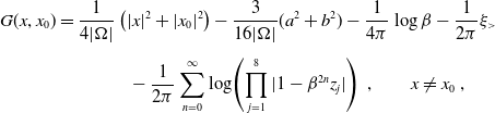 \begin{align} G(x, x_0) & = \dfrac{1}{4|\Omega|}\left( |x|^2 + |x_0|^2 \right) - \dfrac{3}{16|\Omega|}(a^2 + b^2) - \dfrac{1}{4\pi}\log\beta - \dfrac{1}{2\pi}\xi_> \nonumber\\[5pt] & \qquad\qquad - \dfrac{1}{2\pi}\sum^{\infty}_{n=0}\log\!\left( \prod_{j=1}^{8} |1 - \beta^{2n}z_j| \right) \ ,\qquad x \neq x_0 \ ,\end{align}
where a and b are the major and minor axis of the domain, respectively; the area of the domain is $|\Omega| = \pi ab$
, and the parameter
$|\Omega| = \pi ab$
, and the parameter $\beta = (a - b)/(a + b)$
and the values
$\beta = (a - b)/(a + b)$
and the values $\xi_> = \mathop{\textrm{max}}\!(\xi, \xi_0)$
,
$\xi_> = \mathop{\textrm{max}}\!(\xi, \xi_0)$
, $z_1, \ldots, z_8$
are defined in terms of the elliptical coordinates
$z_1, \ldots, z_8$
are defined in terms of the elliptical coordinates $\xi$
and
$\xi$
and $\eta$
as follows.
$\eta$
as follows.
The Cartesian coordinates (x, y) and the elliptical coordinates $(\xi,\eta)$
are related by the transformation:
$(\xi,\eta)$
are related by the transformation:
 \begin{equation} x = f\cosh\xi\cos\eta \ , \quad y = f\sinh\xi\sin\eta \ , \quad f = \sqrt{a^2 - b^2}\,.\end{equation}
For the major and minor axis of the elliptical domain, one has
 \begin{equation} a = f\cosh\xi_b \ , \quad b = f\sinh\xi_b \ , \quad \xi_b = \tanh^{-1}\left(\dfrac{b}{a}\right) = -\dfrac{1}{2}\log\beta.\end{equation}
For the backward transformation, to determine $\xi(x, y)$
, equation (2.9a) is solved to give
$\xi(x, y)$
, equation (2.9a) is solved to give
 \begin{equation}\xi = \dfrac{1}{2}\log\!\left( 1 - 2s + 2\sqrt{s^2 - s} \right) \ , \quad s \equiv \dfrac{-\mu - \sqrt{\mu^2 + 4f^2y^2}}{2f^2} \ , \quad \mu \equiv x^2 + y^2 - f^2\, .\end{equation}
In a similar fashion, $\eta(x, y)$
is found in terms of
$\eta(x, y)$
is found in terms of $\eta_\star \equiv \sin^{-1}(\sqrt{p})$
to be
$\eta_\star \equiv \sin^{-1}(\sqrt{p})$
to be
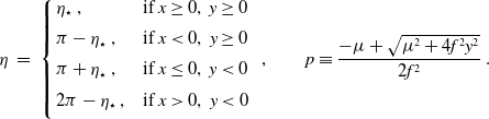 \begin{equation}\eta \ = \ \left\lbrace \begin{array}{l@{\quad}l}\eta_\star \ , & \text{if}\ x \geq 0,\ y \geq 0 \\[5pt]\pi - \eta_\star \ , & \text{if}\ x < 0,\ y \geq 0 \\[5pt]\pi + \eta_\star \ , & \text{if}\ x \leq 0,\ y < 0 \\[5pt]2\pi - \eta_\star \ , & \text{if}\ x > 0,\ y < 0 \\[5pt]\end{array}\right. \ ,\qquad p\equiv \dfrac{-\mu + \sqrt{\mu^2 + 4f^2y^2}}{2f^2}\, .\end{equation}
Finally, the $z_j$
-terms appearing in the infinite sum of equation (2.8) are defined via
$z_j$
-terms appearing in the infinite sum of equation (2.8) are defined via $\xi$
,
$\xi$
, $\eta$
, and
$\eta$
, and $\xi_b$
as:
$\xi_b$
as:
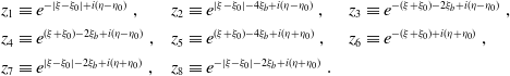 \begin{equation} \begin{array}{l@{\quad}l@{\quad}l}z_1 \equiv e^{-|\xi - \xi_0| + i(\eta - \eta_0)} \ , &z_2 \equiv e^{ |\xi - \xi_0| - 4\xi_b + i(\eta - \eta_0)} \ , &z_3 \equiv e^{-(\xi + \xi_0) - 2\xi_b + i(\eta - \eta_0)} \ , \\[4pt]z_4 \equiv e^{ (\xi + \xi_0) - 2\xi_b + i(\eta - \eta_0)} \ , &z_5 \equiv e^{ (\xi + \xi_0) - 4\xi_b + i(\eta + \eta_0)} \ , &z_6 \equiv e^{-(\xi + \xi_0) + i(\eta + \eta_0)} \ , \\[4pt]z_7 \equiv e^{|\xi - \xi_0| - 2\xi_b + i(\eta + \eta_0)} \ , &z_8 \equiv e^{-|\xi - \xi_0| - 2\xi_b + i(\eta + \eta_0)} \ . &\\\end{array}\end{equation}
The regular part of the Neumann–Green’s function, R, can be expressed in similar terms as G in equation (2.8) but requires a restatement of the $z_j$
-terms given in (2.11). It is given by:
$z_j$
-terms given in (2.11). It is given by:
 \begin{equation} \begin{split}R(x_0) \ = \ & \dfrac{|x_0|^2}{2|\Omega|} \ - \ \dfrac{3}{16|\Omega|}(a^2 + b^2) \ + \ \dfrac{1}{2\pi}\log\!(a + b) \ - \ \dfrac{\xi_0}{2\pi} \ + \ \dfrac{1}{4\pi}\log\!\left( \cosh^2\xi_0 - \cos^2\eta_0 \right) \\[5pt]& \ - \ \dfrac{1}{2\pi}\sum_{n=1}^{\infty}\log\!\left(1 - \beta^{2n}\right) \ - \ \dfrac{1}{2\pi}\sum_{n=0}^{\infty}\log\!\left( \prod_{j=2}^{8}\left|1 - \beta^{2n}z^{0}_j\right| \right).\end{split} \ \end{equation}
Here, $z^{0}_j$
denotes the limiting value of
$z^{0}_j$
denotes the limiting value of $z_j$
, as defined in equation (2.11), as
$z_j$
, as defined in equation (2.11), as $(\xi, \eta) \to (\xi_0, \eta_0)$
, given by:
$(\xi, \eta) \to (\xi_0, \eta_0)$
, given by:
 \begin{equation}\begin{array}{l@{\quad}l@{\quad}l} &z^{0}_2 = \beta^2 \ , &z^{0}_3 = \beta e^{-2\xi_0} \ , \\[5pt]z^{0}_4 = \beta e^{2\xi_0} \ , &z^{0}_5 = \beta^2 e^{2(\xi_0 + i\eta_0)} \ , &z^{0}_6 = e^{2(-\xi_0 + i\eta_0)} \ , \\[5pt]z^{0}_7 = \beta e^{2i\eta_0} \ , &z^{0}_8 = \beta e^{2i\eta_0} \ . &\\\end{array}\end{equation}
3. Global optimisation
In this section, the methods used to find the optimum trap configurations minimising the AMFPT (2.1) are discussed, as are the parameters and constraints used to specify the optimisation problem. We include a description of the general optimisation strategy, the algorithms used, and some implementation details. For the model specification, we discuss the choices of the domain and trap sizes. To conclude, we give some details on the expected accuracy of our approach, to help interpret the results presented later.
3.1. Model parameters
The parameters which defined each optimisation problem were the number of traps N, the sizes of the traps $ \varepsilon_1, \ldots, \varepsilon_N$
, and eccentricity of the elliptic domain given by:
$ \varepsilon_1, \ldots, \varepsilon_N$
, and eccentricity of the elliptic domain given by:
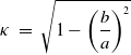 \begin{equation} \kappa \ = \ \sqrt{1 - \left( \dfrac{b}{a} \right)^2}\end{equation}
in terms of the major and the minor semi-axes a and b. We imposed a common requirement that the area of the domain be $|\Omega| = \pi$
to facilitate comparisons of results for different eccentricities.
$|\Omega| = \pi$
to facilitate comparisons of results for different eccentricities.
This study explored the following parameters. We considered domain eccentricities of $\kappa = 0$
,
$\kappa = 0$
, $0.472$
,
$0.472$
, $0.802$
, and
$0.802$
, and $0.995$
, and for
$0.995$
, and for $N \leq 50$
traps. For traps of equal size, we took
$N \leq 50$
traps. For traps of equal size, we took $\varepsilon = 0.05$
in order to facilitate comparison with previous studies [Reference Iyaniwura, Wong, Macdonald and Ward12]. For traps of different sizes (see Section 5 below), we took two traps to be larger than the others. The size of the smaller traps was chosen to be
$\varepsilon = 0.05$
in order to facilitate comparison with previous studies [Reference Iyaniwura, Wong, Macdonald and Ward12]. For traps of different sizes (see Section 5 below), we took two traps to be larger than the others. The size of the smaller traps was chosen to be $\varepsilon_1 = 10^{-9}$
to further reduce the number of computations spent on insufficiently separated traps, and the larger traps were taken to be either
$\varepsilon_1 = 10^{-9}$
to further reduce the number of computations spent on insufficiently separated traps, and the larger traps were taken to be either $\varepsilon_2 = 10^{3}\varepsilon_1$
or
$\varepsilon_2 = 10^{3}\varepsilon_1$
or $\varepsilon_2 = 10^{6}\varepsilon_1$
. The relative difference was chosen to be several orders of magnitude because the trap interactions are weighted by
$\varepsilon_2 = 10^{6}\varepsilon_1$
. The relative difference was chosen to be several orders of magnitude because the trap interactions are weighted by $\nu = -\!\log\!(\varepsilon)^{-1}$
, meaning a significant different in sizes is required to achieve observable effects. The number of larger traps was kept small to limit the computational complexity of the problem, for the following reasons.
$\nu = -\!\log\!(\varepsilon)^{-1}$
, meaning a significant different in sizes is required to achieve observable effects. The number of larger traps was kept small to limit the computational complexity of the problem, for the following reasons.
For traps of different sizes, it was found that the computational problem was significantly complicated by the fact that the optimal placement of a trap now depended on its size, leading to the loss of some advantageous symmetry, in a similar way that changing the eccentricity of the domain eliminates the rotational invariance of a configuration. To account for this we used an optimised configuration, obtained for identical traps, as an initial guess, then applied our method for all unique combinations of initial trap locations. With this approach, for N total traps and m traps of a different size than the others, there are $C_N^m = N! / (m!(N-m)!) \sim \mathcal{O}(N^m/m!)$
initial configurations to consider. To maintain relative computational simplicity, the study was limited to
$C_N^m = N! / (m!(N-m)!) \sim \mathcal{O}(N^m/m!)$
initial configurations to consider. To maintain relative computational simplicity, the study was limited to $N = 5$
,
$N = 5$
, $N = 10$
, and
$N = 10$
, and $m = 2$
.
$m = 2$
.
3.2. Model constraints
In terms of the optimisation constraints, we note that the asymptotic approximation of the AMFPT used in this work was derived under the assumptions of the traps being well separated, and small relative to the domain: $\varepsilon \ll 1$
. Special care needed to be taken to ensure that the traps were well separated. If the traps were to come into contact or overlap, the asymptotic equation (2.1) could yield non-physical values
$\varepsilon \ll 1$
. Special care needed to be taken to ensure that the traps were well separated. If the traps were to come into contact or overlap, the asymptotic equation (2.1) could yield non-physical values $\overline{u}_0 < 0$
(a common feature of asymptotic formulas that replace finite traps with ‘point traps’ in various narrow escape and narrow capture setups). In the MFPT optimisation, the traps are effectively repelled from one another, as well as from their ‘reflections’ in the domain boundary. For example, for the disc domain, this is manifested in the fact that the Green’s function (2.7a) grows logarithmically as
$\overline{u}_0 < 0$
(a common feature of asymptotic formulas that replace finite traps with ‘point traps’ in various narrow escape and narrow capture setups). In the MFPT optimisation, the traps are effectively repelled from one another, as well as from their ‘reflections’ in the domain boundary. For example, for the disc domain, this is manifested in the fact that the Green’s function (2.7a) grows logarithmically as $x\to x_0$
as well as when
$x\to x_0$
as well as when $|x|\to 1$
. In particular, q increases as distance between traps decreases, yet as traps begin to overlap q decreases extremely rapidly, appearing to the optimisation algorithm to give a favourable configuration. Though this problem can be addressed by artificially assigning q a high value when an unacceptable configuration is encountered, this approach was found to significantly reduce the efficiency of the global search. Instead, an optimum was first found for
$|x|\to 1$
. In particular, q increases as distance between traps decreases, yet as traps begin to overlap q decreases extremely rapidly, appearing to the optimisation algorithm to give a favourable configuration. Though this problem can be addressed by artificially assigning q a high value when an unacceptable configuration is encountered, this approach was found to significantly reduce the efficiency of the global search. Instead, an optimum was first found for $\varepsilon = 0$
, following which a local search was carried out using these coordinates as an initial guess, and further optimisation applied from there on.
$\varepsilon = 0$
, following which a local search was carried out using these coordinates as an initial guess, and further optimisation applied from there on.
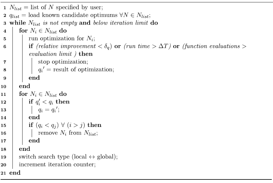
3.3. Method description
In all cases the same general approach, outlined in Algorithm 1, was taken to find the putative optimal trap configuration for a given set of model parameters. The optimisation method had three components, referred to as sweep, iteration, and search. A ‘search’ consisted of running an optimisation algorithm for a specific N, an ‘iteration’ consisted of comparisons of the results of each search and selecting which values of N should considered in subsequent searches, and a ‘sweep’ consisted of a series of iterations. After each iteration, the search would alternate between the global and local algorithms, described below. Each search would run until one of three stopping conditions was encountered. The first of these was
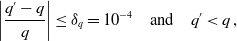 \begin{equation} \left|\dfrac{q' - q}{q}\right| \leq \delta_q = 10^{-4} \quad \text{and} \quad q' < q\,,\end{equation}
meaning that the new candidate optimal value q
′ of the merit function (2.6) did not provide a sufficiently large relative improvement. The second condition was that the execution time of the program exceeded 30 min, and the third was that the number of merit function evaluations exceeded $ 10^{6} $
. After the search was conducted for each N, the results were compared to previous results according to two criteria. The first of these was that, for a specific
$ 10^{6} $
. After the search was conducted for each N, the results were compared to previous results according to two criteria. The first of these was that, for a specific $ N_i $
from the list,
$ N_i $
from the list, $ {q_i}' < q_i $
, meaning that an improvement had been made. The second was that
$ {q_i}' < q_i $
, meaning that an improvement had been made. The second was that $ q_i $
was consistent with the expectation that q must be a decreasing function of N, as we expect the AMFPT to decrease as more traps are added. If both of these conditions were satisfied, the new interim optimum was accepted and
$ q_i $
was consistent with the expectation that q must be a decreasing function of N, as we expect the AMFPT to decrease as more traps are added. If both of these conditions were satisfied, the new interim optimum was accepted and $ N_i $
would not be considered in further iterations. Iterations would repeat until the list was exhausted, a user-defined limit was exceeded, or the program was manually stopped. On each new sweep, the list would be repopulated and the process would repeat, informed by the newly obtained optimums. For traps of different sizes, permutation of trap positions occurred after each sweep.
$ N_i $
would not be considered in further iterations. Iterations would repeat until the list was exhausted, a user-defined limit was exceeded, or the program was manually stopped. On each new sweep, the list would be repopulated and the process would repeat, informed by the newly obtained optimums. For traps of different sizes, permutation of trap positions occurred after each sweep.
Algorithm 1: Pseudocode for the general form of the optimization method used here.
3.4. Choice of algorithms
The global search employed the particle swarm algorithm PSwarm [Reference Ismael F. Vaz and Vicente11], as implemented in the freely available software package OPTI [Reference Currie, Wilson, Sahinidis and Pinto6]. The default values for the social and cognitive parameters were chosen, meaning the local optimum known by each particle tended to be as attractive as the known global optimum. These values were chosen with the intent that the parameter space would be explored as broadly as possible. For the local search, the Nelder–Mead algorithm [Reference Lagarias, Reeds, Wright and Wright16], as implemented in MATLAB R2020, was used. The algorithms were chosen based on their broad applicability, availability in software libraries, and the fact that they do not require information about the structure of the merit function, such as its partial derivatives. Algorithms with such properties are commonly referred to as derivative-free (see, e.g., [Reference Rios and Sahinidis22]).
3.5. Expected accuracy of results
Concerning the accuracy of results, we note that the error associated with the AMFPT and q (2.6) is $\mathcal{O}(\varepsilon^2)$
[Reference Iyaniwura, Wong, Macdonald and Ward12]. For the largest trap size considered in this study,
$\mathcal{O}(\varepsilon^2)$
[Reference Iyaniwura, Wong, Macdonald and Ward12]. For the largest trap size considered in this study, $\varepsilon = 0.05$
, this means that
$\varepsilon = 0.05$
, this means that $ \delta_q = 0.0025 $
, which motivated the choice of stopping threshold
$ \delta_q = 0.0025 $
, which motivated the choice of stopping threshold $\delta_q$
(3.2). While in the current elliptic domain setup, the Green’s function is known explicitly in terms of a series (2.12a) which can be summed numerically to an arbitrary precision accessible to software. In a more general case, where entries of the Green’s matrix
$\delta_q$
(3.2). While in the current elliptic domain setup, the Green’s function is known explicitly in terms of a series (2.12a) which can be summed numerically to an arbitrary precision accessible to software. In a more general case, where entries of the Green’s matrix $\mathcal{G}$
might be known only approximately, with some expected relative error
$\mathcal{G}$
might be known only approximately, with some expected relative error $\delta_G$
, the resulting relative error in the merit function may reach the values
$\delta_G$
, the resulting relative error in the merit function may reach the values $\sim N^2 \delta_G$
. In such a case, in order to use the threshold value
$\sim N^2 \delta_G$
. In such a case, in order to use the threshold value $\delta_q$
in (3.2), one would need to compute the the Green’s matrix entries with relative error
$\delta_q$
in (3.2), one would need to compute the the Green’s matrix entries with relative error $\delta_G\lesssim N^{-2} \delta_q$
.
$\delta_G\lesssim N^{-2} \delta_q$
.
4. Optimisation results: N identical traps
In this section, we use the method outlined in Section 3 to compute putative global optimum configurations of N equal traps in the ellipse, $1\leq N\leq 50$
, compare these results of this study to previous results for the unit disk [Reference Kolokolnikov, Titcombe and Ward14], and present some analysis of the trap configurations. In particular, we show that the unit disc AMFPT values for the putative optimal configurations found below are consistently better than those given in [Reference Kolokolnikov, Titcombe and Ward14].
$1\leq N\leq 50$
, compare these results of this study to previous results for the unit disk [Reference Kolokolnikov, Titcombe and Ward14], and present some analysis of the trap configurations. In particular, we show that the unit disc AMFPT values for the putative optimal configurations found below are consistently better than those given in [Reference Kolokolnikov, Titcombe and Ward14].
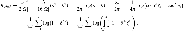
Though it is conventional to discuss optimal configurations in terms of their ‘interaction energy’ used as the merit function (see, e.g., [Reference Ridgway and Cheviakov21] and references therein), here we will use the full asymptotic AMFPT expression [Reference Iyaniwura, Wong, Macdonald and Ward12, Reference Kolokolnikov, Titcombe and Ward14]:
 \begin{equation}\overline{u}_0 \ = \ \dfrac{|\Omega|}{2\pi D\nu N}\left( 1 + \dfrac{4\pi^2 D \nu}{|\Omega|}\textbf{e}^{T}\mathcal{G} \mathcal{A} \right).\end{equation}
which facilitates comparisons with the previous work [Reference Kolokolnikov, Titcombe and Ward14] in the case of the unit disk. We denote the AMFPT values of the trap arrangements found in [Reference Kolokolnikov, Titcombe and Ward14] by $\tilde{u}_0$
. Table 1 compares
$\tilde{u}_0$
. Table 1 compares $\tilde{u}_0$
and
$\tilde{u}_0$
and $\overline{u}_0$
(4.1) for each N reported in the previous study ([Reference Kolokolnikov, Titcombe and Ward14], Table 2). It can be seen that the new values are consistently smaller, differing at most in the third significant figure. A plot of the difference between the previous and the new putative optimal AMFPT values, relative to the previous results, is presented in Figure 2.
$\overline{u}_0$
(4.1) for each N reported in the previous study ([Reference Kolokolnikov, Titcombe and Ward14], Table 2). It can be seen that the new values are consistently smaller, differing at most in the third significant figure. A plot of the difference between the previous and the new putative optimal AMFPT values, relative to the previous results, is presented in Figure 2.

Figure 2. Relative difference $(\overline{u}_0 - \tilde{u}_0)/\tilde{u}_0$
between average MFPT
$(\overline{u}_0 - \tilde{u}_0)/\tilde{u}_0$
between average MFPT $\tilde{u}_0$
in the unit disc for previously found putative optimal configurations ([Reference Kolokolnikov, Titcombe and Ward14], Table 2) and the optimal average MFPT values
$\tilde{u}_0$
in the unit disc for previously found putative optimal configurations ([Reference Kolokolnikov, Titcombe and Ward14], Table 2) and the optimal average MFPT values $\overline{u}_0$
(4.1) computed in this work (Table 1).
$\overline{u}_0$
(4.1) computed in this work (Table 1).
Table 1. Average MFPT $\tilde{u}_0$
in the unit disc for previously computed putative optimal configurations ([Reference Kolokolnikov, Titcombe and Ward14], Table 2) compared to the AMFPT
$\tilde{u}_0$
in the unit disc for previously computed putative optimal configurations ([Reference Kolokolnikov, Titcombe and Ward14], Table 2) compared to the AMFPT $\overline{u}_0$
(4.1) for optimal trap arrangements computed in this work. The relative difference plot is given in Figure 2
$\overline{u}_0$
(4.1) for optimal trap arrangements computed in this work. The relative difference plot is given in Figure 2

The computed optimal values of the merit function (2.6) that correspond to putative globally optimal minima of the AMFPT (2.1), for the domain eccentricities $\kappa = 0$
(circular disc),
$\kappa = 0$
(circular disc), $0.472$
,
$0.472$
, $0.802$
, and
$0.802$
, and $0.995$
, are presented in Table 2 below and are graphically shown in Figure 3. While the first three plots are nearly identical, the plot (d) for the largest eccentricity value differs significantly for small N but becomes similar to the other plots for larger N.
$0.995$
, are presented in Table 2 below and are graphically shown in Figure 3. While the first three plots are nearly identical, the plot (d) for the largest eccentricity value differs significantly for small N but becomes similar to the other plots for larger N.

Table 2. Optimised values of the merit function (2.6), for each number of traps N and eccentricity $\kappa$
considered in this study. Plots of these values are found in Figure 3
$\kappa$
considered in this study. Plots of these values are found in Figure 3

Plots comparing the optimal configurations of select N for each of the eccentricities considered in this study are shown in Figures 4–7. Each plot shows the positions of the traps within the domain, along with a visualisation of a Delaunay triangulation [Reference Lee and Schachter17] calculated using the traps as vertices, to illustrate the distribution of the traps and relative distance between them.

Figure 4. Plots depicting optimal trap distribution for $N=5$
, comparing eccentricities of (a)
$N=5$
, comparing eccentricities of (a) $\kappa = 0$
, (b)
$\kappa = 0$
, (b) $\kappa = 0.472$
, (c)
$\kappa = 0.472$
, (c) $\kappa = 0.802$
, and (d)
$\kappa = 0.802$
, and (d) $\kappa = 0.995$
. For each subfigure (a)–(d), upper plots show positions of traps, along with a visualisation of nearest-neighbour pairs calculated using Delaunay triangulation. Lower plots show the scaling factor given by the equation (4.2).
$\kappa = 0.995$
. For each subfigure (a)–(d), upper plots show positions of traps, along with a visualisation of nearest-neighbour pairs calculated using Delaunay triangulation. Lower plots show the scaling factor given by the equation (4.2).

Figure 5. Plots depicting optimal trap distribution for $N=10$
, comparing eccentricities of (a)
$N=10$
, comparing eccentricities of (a) $\kappa = 0$
, (b)
$\kappa = 0$
, (b) $\kappa = 0.472$
, (c)
$\kappa = 0.472$
, (c) $\kappa = 0.802$
, and (d)
$\kappa = 0.802$
, and (d) $\kappa = 0.995$
. For each subfigure (a)–(d), upper plots show positions of traps, along with a visualisation of nearest-neighbour pairs calculated using Delaunay triangulation. Lower plots show the scaling factor given by the equation (4.2).
$\kappa = 0.995$
. For each subfigure (a)–(d), upper plots show positions of traps, along with a visualisation of nearest-neighbour pairs calculated using Delaunay triangulation. Lower plots show the scaling factor given by the equation (4.2).

Figure 6. Plots depicting optimal trap distribution for $N=25$
, comparing eccentricities of (a)
$N=25$
, comparing eccentricities of (a) $\kappa = 0$
, (b)
$\kappa = 0$
, (b) $\kappa = 0.472$
, (c)
$\kappa = 0.472$
, (c) $\kappa = 0.802$
, and (d)
$\kappa = 0.802$
, and (d) $\kappa = 0.995$
. For each subfigure (a)–(d), upper plots show positions of traps, along with a visualisation of nearest-neighbour pairs calculated using Delaunay triangulation. Lower plots show the scaling factor given by the equation (4.2).
$\kappa = 0.995$
. For each subfigure (a)–(d), upper plots show positions of traps, along with a visualisation of nearest-neighbour pairs calculated using Delaunay triangulation. Lower plots show the scaling factor given by the equation (4.2).

Figure 7. Plots depicting optimal trap distribution for $N=40$
, comparing eccentricities of (a)
$N=40$
, comparing eccentricities of (a) $\kappa = 0$
, (b)
$\kappa = 0$
, (b) $\kappa = 0.472$
, (c)
$\kappa = 0.472$
, (c) $\kappa = 0.802$
, and (d)
$\kappa = 0.802$
, and (d) $\kappa = 0.995$
. For each subfigure (a)–(d), upper plots show positions of traps, along with a visualisation of nearest-neighbour pairs calculated using Delaunay triangulation. Lower plots show the scaling factor given by the equation (4.2).
$\kappa = 0.995$
. For each subfigure (a)–(d), upper plots show positions of traps, along with a visualisation of nearest-neighbour pairs calculated using Delaunay triangulation. Lower plots show the scaling factor given by the equation (4.2).
In addition, it was of interest to see how the ring-like distribution of traps would change with the eccentricity of the domain. This is related to the observation that for the unit disc, optimal trap configurations tend to form ring-like structures [Reference Kolokolnikov, Titcombe and Ward14]; a similar effect is observed for the MFPT problem with internal traps in the unit sphere, where equal traps tend to be centred close to nested spherical surfaces [Reference Gilbert and Cheviakov7]. To be specific, traps on a ring would have common radial coordinates and common angular separation from their neighbours on the ring. Ring-like distributions would then be ones which are qualitatively similar to a ring.
In order to examine the configurations for ring-like structure, visualisations of the effective radial coordinates of the traps were produced. To elaborate, a scaling factor was calculated for each trap which corresponds to the size of the elliptical contour which that trap would be placed. This scaling factor c is given by the equation:
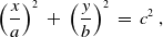 \begin{equation} \left( \dfrac{x}{a} \right)^2 \ + \ \left( \dfrac{y}{b} \right)^2 \ = \ c^2 \, ,\end{equation}
where $c = 1$
corresponds to the boundary of the domain. When the domain is circular, meaning
$c = 1$
corresponds to the boundary of the domain. When the domain is circular, meaning $a = b = 1$
, then in terms of polar coordinates, c is the radial coordinate of the trap. It should be kept in mind that these measures are meant as a rough criteria to test the prevalence of ring-like configurations. A more thorough examination would require the traps be categorised by their radial proximity to one another, following which the angular coordinates of alike traps would be compared. The scaling factors are shown in the lower subplots in Figures 4–7. For the case of
$a = b = 1$
, then in terms of polar coordinates, c is the radial coordinate of the trap. It should be kept in mind that these measures are meant as a rough criteria to test the prevalence of ring-like configurations. A more thorough examination would require the traps be categorised by their radial proximity to one another, following which the angular coordinates of alike traps would be compared. The scaling factors are shown in the lower subplots in Figures 4–7. For the case of $N=5$
, Figure 4 can be compared to the optimal configurations presented in [Reference Iyaniwura, Wong, Macdonald and Ward12], through which it can be seen that the two are qualitatively similar and exhibit the same relationship between trap distribution and domain eccentricity. For higher eccentricity values (except the degenerate cases where traps lie on the symmetry axis: Figures 4(d), 5(d)), the trap configurations do not tend to show ring-like structures that are present, to some degree, in the disc and low-eccentricity elliptic domains.
$N=5$
, Figure 4 can be compared to the optimal configurations presented in [Reference Iyaniwura, Wong, Macdonald and Ward12], through which it can be seen that the two are qualitatively similar and exhibit the same relationship between trap distribution and domain eccentricity. For higher eccentricity values (except the degenerate cases where traps lie on the symmetry axis: Figures 4(d), 5(d)), the trap configurations do not tend to show ring-like structures that are present, to some degree, in the disc and low-eccentricity elliptic domains.
To examine the putative optimal distributions of traps in terms of their pairwise distance to the closest neighbour and related measures, a Delaunay triangulation was computed to identify neighbours of each trap (see upper plots in Figures 4–7). In general, for a configuration of N traps distributed, in some sense, ‘uniformly’ over the elliptic domain of area $|\Omega| = \pi$
, the average ‘area per trap’ is given by
$|\Omega| = \pi$
, the average ‘area per trap’ is given by $A(N) = |\Omega|/N = \pi/N$
. Likening an optimal arrangement of N traps to a collection of circles packed into an enclosed space, the (average) distance
$A(N) = |\Omega|/N = \pi/N$
. Likening an optimal arrangement of N traps to a collection of circles packed into an enclosed space, the (average) distance $\langle d\rangle$
between two neighbouring traps would be the distance between the centres of two identical circles representing the area occupied by each trap; it would be related to the area per trap as
$\langle d\rangle$
between two neighbouring traps would be the distance between the centres of two identical circles representing the area occupied by each trap; it would be related to the area per trap as $A(N)= \pi\langle d\rangle^2 / 4$
. One consequently finds that the average distance between neighbouring traps, equivalent to the diameter of one of the circles, is given by:
$A(N)= \pi\langle d\rangle^2 / 4$
. One consequently finds that the average distance between neighbouring traps, equivalent to the diameter of one of the circles, is given by:
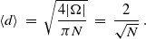 \begin{equation} \langle d \rangle \ = \ \sqrt{\dfrac{4 |\Omega|}{\pi N}} \ = \ \dfrac{2}{\sqrt{N}}\,.\end{equation}
Extending this comparison to the traps nearest the boundary, the smallest distance between a trap and the boundary was taken to be the radius of a circle surrounding the trap, and the diameter of this circle was compared to the smallest distance between two traps. This essentially provides a measure of the distance between a near-the-boundary trap and its ‘reflection’ in the Neumann boundary.
In Figure 8, for each of the four considered eccentricities of the elliptic domain, the mean pairwise distance between neighbouring traps is plotted as a function of N, along with minimum pairwise distance between traps, and $2\times$
minimal distance to the boundary. These are compared with the average distance formula (4.3) coming from the ‘area per trap’ argument. It can be observed that the simple formula (4.3) may be used as a reasonable estimate of common pairwise distances between traps in an optimal configuration.
$2\times$
minimal distance to the boundary. These are compared with the average distance formula (4.3) coming from the ‘area per trap’ argument. It can be observed that the simple formula (4.3) may be used as a reasonable estimate of common pairwise distances between traps in an optimal configuration.

Figure 8. Plots depicting local pairwise distance properties of optimal trap distributions as functions of N, for domain eccentricities $\kappa = 0$
(a),
$\kappa = 0$
(a), $\kappa = 0.472$
(b),
$\kappa = 0.472$
(b), $\kappa = 0.802$
(c), and
$\kappa = 0.802$
(c), and $\kappa = 0.995$
(d). The curve entitled ‘Measure of Area per Trap’ shows the distance
$\kappa = 0.995$
(d). The curve entitled ‘Measure of Area per Trap’ shows the distance $\langle d \rangle$
computed using the ‘area per trap’ argument and the resulting formula (4.3).
$\langle d \rangle$
computed using the ‘area per trap’ argument and the resulting formula (4.3).
5. Traps of different sizes
We now consider the case when the small traps are circular and well separated but have differing sizes given by $\varepsilon_j$
,
$\varepsilon_j$
, $j=1,\ldots, N$
, with the corresponding size parameters
$j=1,\ldots, N$
, with the corresponding size parameters $\nu_j = -1/\log\varepsilon_j$
. In the case of same or different-sized traps, the leading-term MFPT contribution satisfies [Reference Iyaniwura, Wong, Macdonald and Ward12, Reference Kurella, Tzou, Coombs and Ward15]
$\nu_j = -1/\log\varepsilon_j$
. In the case of same or different-sized traps, the leading-term MFPT contribution satisfies [Reference Iyaniwura, Wong, Macdonald and Ward12, Reference Kurella, Tzou, Coombs and Ward15]
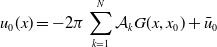 \begin{equation*}u_0(x)=-2\pi\sum_{k=1}^{N}\mathcal{A}_k G(x, x_0) + \bar{u}_0\end{equation*}
and, when matched with the far-field behaviour of $u_0$
, yields
$u_0$
, yields
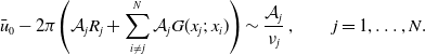 \begin{equation}\bar{u}_0 - 2\pi \!\left(\mathcal{A}_j R_j + \sum_{i \neq j}^{N} \mathcal{A}_j G(x_j ;\; x_i)\right)\sim \dfrac{\mathcal{A}_j}{\nu_j}\,, \qquad j=1,\ldots, N.\end{equation}
When all $\nu_j=\nu$
, the matching condition (5.1) and (2.2) yield the formulas (2.1) and (2.3). In the general case, the equations (5.1) and (2.2) can also be solved explicitly. One obtains
$\nu_j=\nu$
, the matching condition (5.1) and (2.2) yield the formulas (2.1) and (2.3). In the general case, the equations (5.1) and (2.2) can also be solved explicitly. One obtains
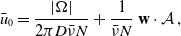 \begin{equation}\bar{u}_0=\dfrac{|\Omega|}{2\pi D \bar{\nu} N} + \dfrac{1}{\bar{\nu} N}\,{\boldsymbol{\rm {w}}}\cdot \mathcal{A}\,,\end{equation}
where the vector $\mathcal{A}$
is the solution of the linear system:
$\mathcal{A}$
is the solution of the linear system:
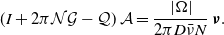 \begin{equation}(I+2\pi \mathcal{N} \mathcal{G}-\mathcal{Q})\,\mathcal{A}=\dfrac{|\Omega|}{2\pi D \bar{\nu} N} \,{\boldsymbol{\rm {\nu}}}.\end{equation}
In (5.2) and (5.3), $\mathcal{G}$
is the Green’s matrix (2.4),
$\mathcal{G}$
is the Green’s matrix (2.4), ${\boldsymbol{\rm {\nu}}}=(\nu_1,\ldots, \nu_N)^T$
is the trap size parameter vector,
${\boldsymbol{\rm {\nu}}}=(\nu_1,\ldots, \nu_N)^T$
is the trap size parameter vector, $\mathcal{N}={\rm diag}\,{\boldsymbol{\rm {\nu}}}$
is the corresponding diagonal
$\mathcal{N}={\rm diag}\,{\boldsymbol{\rm {\nu}}}$
is the corresponding diagonal $N\times N$
matrix,
$N\times N$
matrix, $\bar{\nu}=\left(\sum_{i=1}^{N}\,\nu_j\right)/N$
is the average trap size parameter,
$\bar{\nu}=\left(\sum_{i=1}^{N}\,\nu_j\right)/N$
is the average trap size parameter, ${\boldsymbol{\rm {w}}} = 2\pi {\boldsymbol{\rm {e}}}^T\mathcal{N}\mathcal{G}$
is a row vector, and
${\boldsymbol{\rm {w}}} = 2\pi {\boldsymbol{\rm {e}}}^T\mathcal{N}\mathcal{G}$
is a row vector, and $\mathcal{Q}=({\boldsymbol{\rm {\nu}}}\cdot {\boldsymbol{\rm {w}}})/(\bar{\nu} N)$
is an
$\mathcal{Q}=({\boldsymbol{\rm {\nu}}}\cdot {\boldsymbol{\rm {w}}})/(\bar{\nu} N)$
is an $N\times N$
matrix.
$N\times N$
matrix.
The optimisation of the approximate AMFPT (5.2) corresponds to the optimisation of the second term of (5.2), or equivalently, the merit function:
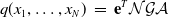 \begin{equation} q(x_1,\ldots,x_N) \ = \ {\boldsymbol{\rm {e}}}^T\mathcal{N}\mathcal{G} \mathcal{A} \ \end{equation}
depending on 2N scalar variables. The expression (5.4) generalises the merit function (2.6) onto the set-up with non-equal traps.
As an illustration, we consider elliptic domains with $N=N_1+N_2$
traps, such that
$N=N_1+N_2$
traps, such that $N_1$
traps have common radii
$N_1$
traps have common radii $\varepsilon_1$
, and
$\varepsilon_1$
, and $N_2$
traps common radii
$N_2$
traps common radii $\varepsilon_2>\varepsilon_1$
. Using the global optimisation procedure described in Section 3 and the values
$\varepsilon_2>\varepsilon_1$
. Using the global optimisation procedure described in Section 3 and the values $\varepsilon_1 = 10^{-9}$
and
$\varepsilon_1 = 10^{-9}$
and $\varepsilon_2 = 10^{3}\varepsilon_1$
or
$\varepsilon_2 = 10^{3}\varepsilon_1$
or $\varepsilon_2 = 10^{6}\varepsilon_1$
, the configurations obtained for two different values of eccentricity
$\varepsilon_2 = 10^{6}\varepsilon_1$
, the configurations obtained for two different values of eccentricity $\kappa = 0.472$
or
$\kappa = 0.472$
or $\kappa = 0.802$
and the trap numbers
$\kappa = 0.802$
and the trap numbers $N_2=2$
and
$N_2=2$
and $N=5, 10$
are shown in Figures 9 and 10. As expected, larger traps produce a stronger ‘push’ than the smaller ones. It is evident that the increase of the
$N=5, 10$
are shown in Figures 9 and 10. As expected, larger traps produce a stronger ‘push’ than the smaller ones. It is evident that the increase of the $\varepsilon_2/\varepsilon_1$
ratio causes a significant change in the form of the configuration.
$\varepsilon_2/\varepsilon_1$
ratio causes a significant change in the form of the configuration.

Figure 9. Plots depicting optimal trap distributions for $N=5$
traps with three traps of radius
$N=5$
traps with three traps of radius $\varepsilon_1 = 10^{-9}$
and two larger traps of radius
$\varepsilon_1 = 10^{-9}$
and two larger traps of radius $\varepsilon_2 = 10^{3}\varepsilon_1$
(upper) or
$\varepsilon_2 = 10^{3}\varepsilon_1$
(upper) or $\varepsilon_2 = 10^{6}\varepsilon_1$
(lower), and
$\varepsilon_2 = 10^{6}\varepsilon_1$
(lower), and $\kappa = 0.472$
(left) or
$\kappa = 0.472$
(left) or $\kappa = 0.802$
(right). Upper plots show positions of traps along with a crude visualisation of nearest-neighbour pairs calculated using Delaunay triangulation. Lower plots show the scaling factor given by equation (4.2).
$\kappa = 0.802$
(right). Upper plots show positions of traps along with a crude visualisation of nearest-neighbour pairs calculated using Delaunay triangulation. Lower plots show the scaling factor given by equation (4.2).

Figure 10. Plots depicting optimal trap distributions for $N=10$
traps with eight traps of radius
$N=10$
traps with eight traps of radius $\varepsilon_1 = 10^{-9}$
and two larger traps of radius
$\varepsilon_1 = 10^{-9}$
and two larger traps of radius $\varepsilon_2 = 10^{3}\varepsilon_1$
(upper) or
$\varepsilon_2 = 10^{3}\varepsilon_1$
(upper) or $\varepsilon_2 = 10^{6}\varepsilon_1$
(lower), and
$\varepsilon_2 = 10^{6}\varepsilon_1$
(lower), and $\kappa = 0.472$
(left) or
$\kappa = 0.472$
(left) or $\kappa = 0.802$
(right). Upper plots show positions of traps along with a crude visualisation of nearest-neighbour pairs calculated using Delaunay triangulation. Lower plots show the scaling factor given by equation (4.2).
$\kappa = 0.802$
(right). Upper plots show positions of traps along with a crude visualisation of nearest-neighbour pairs calculated using Delaunay triangulation. Lower plots show the scaling factor given by equation (4.2).
6. Discussion
At this point, some interpretation of the previously stated results will be presented. This discussion will concern the putative optimal values of the AMFPT (2.1) in elliptic domains with internal traps, values of the related merit function (2.6), the positions of traps within the domain, the bulk measures of trap distribution which were employed, and the configurations of non-identical traps.
To begin, the method of study will be briefly reiterated. In order to study the dependence of optimal trap configurations on both the number of traps and the eccentricity of the elliptic domain, the values of the merit function (2.6) corresponding to the approximate AMFPT (4.1) were minimised for $N \leq 50$
and sample values of the eccentricity (3.1) of 0, 0.472, 0.802, and 0.995, while the area of the ellipse was kept constant,
$N \leq 50$
and sample values of the eccentricity (3.1) of 0, 0.472, 0.802, and 0.995, while the area of the ellipse was kept constant, $|\Omega| = \pi$
. For N traps, the merit function consequently depends on 2N scalar variables. In the search for a global optimum, an iterative approach, which switched between global and local searches, was used (Section 3). The method used here was similar to that of [Reference Iyaniwura, Wong, Macdonald and Ward12], though a different algorithm was used for the local search, as well as in [Reference Gilbert and Cheviakov7] which used a different algorithms than here for both searches. A somewhat different approach was employed in [Reference Iyaniwura, Wong, Ward and Macdonald13], which made use of numerical solutions to the Poisson problem (1.1). In the case of the unit disc, the comparison of the results of this study to those in [Reference Kolokolnikov, Titcombe and Ward14] demonstrated that the optima reported here are consistently an improvement on previous work. In particular, this is due to the removal of the constraint that all traps be located on rings within the domain – see, for example, Figure 5(a) where for
$|\Omega| = \pi$
. For N traps, the merit function consequently depends on 2N scalar variables. In the search for a global optimum, an iterative approach, which switched between global and local searches, was used (Section 3). The method used here was similar to that of [Reference Iyaniwura, Wong, Macdonald and Ward12], though a different algorithm was used for the local search, as well as in [Reference Gilbert and Cheviakov7] which used a different algorithms than here for both searches. A somewhat different approach was employed in [Reference Iyaniwura, Wong, Ward and Macdonald13], which made use of numerical solutions to the Poisson problem (1.1). In the case of the unit disc, the comparison of the results of this study to those in [Reference Kolokolnikov, Titcombe and Ward14] demonstrated that the optima reported here are consistently an improvement on previous work. In particular, this is due to the removal of the constraint that all traps be located on rings within the domain – see, for example, Figure 5(a) where for $N=10$
, trap centres evidently do not lie on concentric rings.
$N=10$
, trap centres evidently do not lie on concentric rings.
Plots of the putative globally optimal merit function values vs. N, for each eccentricity value considered, are found in Figure 3. It follows that the domain eccentricity is a more important factor when there are few traps, but each function behaves similarly as N increases. In particular, as the number of traps N increases, the AMFPT $\overline{u}_0$
(2.1) approaches zero; the merit function q(x) therefore must, as
$\overline{u}_0$
(2.1) approaches zero; the merit function q(x) therefore must, as $N\to \infty$
, approach from above the value
$N\to \infty$
, approach from above the value $-|\Omega| / (4\pi^2 D\nu) \simeq -0.238$
, which agrees with the plots in Figure 3.
$-|\Omega| / (4\pi^2 D\nu) \simeq -0.238$
, which agrees with the plots in Figure 3.
Examination of the positions of traps in the AMFPT-minimising configurations, both visually and in terms of their radial coordinates, gives the impression that the optimal configuration is one which consists of traps placed on the vertices of nested polygons. These polygons, while irregular, seem to possess some consistent structure, including being convex. (It is interesting to note that the optimal configurations of confined interacting points often take similar forms, both in two and three dimensions [Reference Hoare and Pal8, Reference Manoharan, Elsesser and Pine18, Reference Saint Jean, Even and Guthmann24, Reference Sloane, Hardin, Duff and Conway25].) Due to the geometrical symmetries of the ellipse, the optimal configurations are defined uniquely modulo the group $C^2\times C^2$
of reflections with respect to both axes, which includes the rotation by
$C^2\times C^2$
of reflections with respect to both axes, which includes the rotation by $\pi$
. Numerical optimisation algorithms converge to a single specific representative of the equivalent putative globally optimal configurations. For example, for non-symmetric numerically optimal configuration, several traps may be found along the midline of one half (right or left) of the domain. Optimal trap configurations with the same symmetry group as the ellipse were also observed (see, e.g., Figure 5(c)).
$\pi$
. Numerical optimisation algorithms converge to a single specific representative of the equivalent putative globally optimal configurations. For example, for non-symmetric numerically optimal configuration, several traps may be found along the midline of one half (right or left) of the domain. Optimal trap configurations with the same symmetry group as the ellipse were also observed (see, e.g., Figure 5(c)).
In addition to the examination of individual trap positions in each optimised configuration, quantities were calculated using the distances between neighbouring traps, defined using a Delaunay triangulation of the trap coordinates, which served as bulk measures of the distribution of traps in each configuration. Plots of these measures, shown in Figure 8, illustrate that the mean distance between neighbouring traps tends to be close to the diameter of a circle which would occupy the average area of the domain per trap, as in equation (4.3). Additionally, the minimum distance between any two traps tends to be twice the minimum distance between a trap and the domain boundary, which supports the intuitive reasoning that for the boundary value problem (1.1) with interior traps, the Neumann boundary condition on $\partial\Omega$
‘reflects’ each trap, so that under the AMFPT optimisation, every trap tends to ‘repel’ from its reflection in the boundary the same way as it is repelled from other traps.
$\partial\Omega$
‘reflects’ each trap, so that under the AMFPT optimisation, every trap tends to ‘repel’ from its reflection in the boundary the same way as it is repelled from other traps.
In Section 5, the formulas obtained in [Reference Iyaniwura, Wong, Ward and Macdonald13] pertaining to the approximate asymptotic MFPT in an elliptic domain were generalised onto the case of N traps of different sizes, defined by the radii $\varepsilon_j$
,
$\varepsilon_j$
, $j=1,\ldots, N$
. It was shown that that the AMFPT is approximated by (5.2) and can be minimised simultaneously with the merit function (5.4) of 2N scalar trap coordinates. Global optimisation was performed for sample configurations corresponding to all combinations of trap numbers
$j=1,\ldots, N$
. It was shown that that the AMFPT is approximated by (5.2) and can be minimised simultaneously with the merit function (5.4) of 2N scalar trap coordinates. Global optimisation was performed for sample configurations corresponding to all combinations of trap numbers $N = \lbrace 5, 10 \rbrace$
, domain eccentricities
$N = \lbrace 5, 10 \rbrace$
, domain eccentricities $\kappa = \lbrace 0.472, 0.802 \rbrace$
, and trap size relations
$\kappa = \lbrace 0.472, 0.802 \rbrace$
, and trap size relations $\varepsilon_2 = \lbrace 10^{3}\varepsilon_1, 10^{6}\varepsilon_1 \rbrace$
, when two traps had the same radius
$\varepsilon_2 = \lbrace 10^{3}\varepsilon_1, 10^{6}\varepsilon_1 \rbrace$
, when two traps had the same radius $\varepsilon_2$
and
$\varepsilon_2$
and $N-2$
traps the radius
$N-2$
traps the radius $\varepsilon_1$
. The respective putative optimal configurations shown in Figures 9–10 were obtained. In particular, strong dependence of the form of the optimal configuration on the trap size ratio was observed.
$\varepsilon_1$
. The respective putative optimal configurations shown in Figures 9–10 were obtained. In particular, strong dependence of the form of the optimal configuration on the trap size ratio was observed.
Both in the case of same and different trap sizes, multiple N-trap configurations corresponding to local minima of the AMFPT exist, some having rather close values of the merit function. Computation and analysis of the structure of such local minima, possibly along the lines of a similar study for traps on the surface of the sphere [Reference Ridgway and Cheviakov21], is a possible direction of future research.
In future work, it would also be of interest to address the following related problems. The first is to carry out similar investigations for non-elliptic near-disc domains considered in [Reference Iyaniwura, Wong, Macdonald and Ward12]. Another interesting direction is the development of a scaling law which would predict the behaviour of the MFPT as the number of traps increases with their positions defined according to a specific distribution, in particular, for distributions that globally or locally minimise MFPT, or other distributions of practical significance. A similar problem, along with the dilute trap fraction limit of homogenisation theory, was addressed in [Reference Cheviakov, Ward and Straube4, Reference Cheviakov and Zawada5] for the narrow escape problem involving boundary traps located on the surface of a sphere in three dimensions.
Acknowledgements
A. C. is thankful to NSERC of Canada for research support through the Discovery grant RGPIN-2019-05570.
Conflict of interests
None


 Open access