

1. Introduction
KPP–Fisher reaction diffusion equations $u_t=\Delta u+f(u)$
are fundamental in the modelling of population growths [Reference Fisher10, Reference Murray29], by assuming either the reaction term as the monostable nonlinearity (e.g.
$u_t=\Delta u+f(u)$
are fundamental in the modelling of population growths [Reference Fisher10, Reference Murray29], by assuming either the reaction term as the monostable nonlinearity (e.g. $f(u)= u(1-u)$
) or otherwise the bistable topological structure (e.g.
$f(u)= u(1-u)$
) or otherwise the bistable topological structure (e.g. $f(u)=u(a-u)(1-u)$
,
$f(u)=u(a-u)(1-u)$
, $0\lt a\lt 1$
). A natural and interesting question is: can a system exhibit rich dynamics by combining both monostable and bistable topological properties with just a switch of a impacting parameter? If so, how does the spatial spreading or invasion behave in view of the parameter? How to determine and estimate the moving speeds of the pushed waves, pulled waves or bistable waves?
$0\lt a\lt 1$
). A natural and interesting question is: can a system exhibit rich dynamics by combining both monostable and bistable topological properties with just a switch of a impacting parameter? If so, how does the spatial spreading or invasion behave in view of the parameter? How to determine and estimate the moving speeds of the pushed waves, pulled waves or bistable waves?
To answer the above questions, we consider the following Belousov–Zhabotinsky (BZ for short) reaction-diffusion system
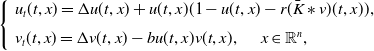 \begin{equation} \left \{ \begin{array}{cc} \begin{aligned} &u_t(t,x)=\Delta u(t,x)+u(t,x)(1-u(t,x)-r(\bar K*v)(t,x)),\\[3pt] &v_t(t,x)=\Delta v(t,x)-bu(t,x)v(t,x), \ \ \ \ \ x\in \mathbb{R}^n,\\ \end{aligned} \end{array} \right . \end{equation}
which builds upon J.D. Murray’s investigations of bio-reaction in [Reference Murray28, Reference Murray29]. The variables $u$
and
$u$
and $v$
represent the bromous acid and bromide ion concentrations, respectively. Here
$v$
represent the bromous acid and bromide ion concentrations, respectively. Here $\Delta$
is the Laplace operator, and
$\Delta$
is the Laplace operator, and $r$
and
$r$
and $b$
are positive reaction parameters. The term
$b$
are positive reaction parameters. The term $\bar K*v$
denote the convolution of the component
$\bar K*v$
denote the convolution of the component $v$
with a nonnegative normalised kernel
$v$
with a nonnegative normalised kernel $\bar K(s,y), s\ge 0, y\in \mathbb{R}^n$
, which satisfies the following conditions:
$\bar K(s,y), s\ge 0, y\in \mathbb{R}^n$
, which satisfies the following conditions:
-
(K1) $\int _{0}^{\infty }\int _{\mathbb{R}^n}\bar K(s,y)dyds=1$
,
$\int _{0}^{\infty }\int _{\mathbb{R}^n}\bar K(s,y)dyds=1$
, -
(K2) There exists
$\tilde{\delta }_0\in (0,\infty )$
such that
$\int _{0}^{\infty }\int _{\mathbb{R}^n}\bar K(s,y)e^{\rho s}dyds\lt \infty$
for
$\rho \in [0, \tilde{\delta }_0)$
.


Let $u=\phi$
and
$u=\phi$
and $v=1-\psi$
. System (1.1) becomes
$v=1-\psi$
. System (1.1) becomes
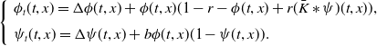 \begin{equation} \left \{ \begin{array}{cc} \begin{aligned} &\phi _t(t,x)=\Delta \phi (t,x)+\phi (t,x)(1-r-\phi (t,x)+r(\bar K*\psi )(t,x)),\\[3pt] &\psi _t(t,x)=\Delta \psi (t,x)+b\phi (t,x)(1-\psi (t,x)).\\ \end{aligned} \end{array} \right . \end{equation}
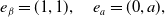
Note that system (1.2) has infinite number of constant equilibria
 \begin{equation} \boldsymbol e_\beta =(1,1), \quad e_a=(0,a), \end{equation}
where $a$
is an arbitrary constant. We may only consider
$a$
is an arbitrary constant. We may only consider $0 \le a \le 1$
so that
$0 \le a \le 1$
so that $(0,a)$
are bounded by
$(0,a)$
are bounded by $e_\beta$
. If
$e_\beta$
. If $a=0$
, then
$a=0$
, then $e_0=(0,0)$
. The kinetic system of model (1.2) is
$e_0=(0,0)$
. The kinetic system of model (1.2) is
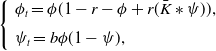 \begin{equation} \left \{ \begin{array}{cc} \begin{aligned} &\phi _t=\phi (1-r-\phi +r(\bar K*\psi )),\\[3pt] &\psi _t=b\phi (1-\psi ),\\ \end{aligned} \end{array} \right . \end{equation}
where $\bar{K}*\psi =\int _{0}^{+\infty }\int _{\mathbb{R}^n}\bar{K}(s,y)\psi (t-s)dyds$
. It can be noted that the conventional definition of monostability/bistability in [Reference Volpert, Volpert and Volpert34] requires a clarification to system (1.2) that possesses a continuum of non-negative equilibria. The stability analysis of (1.4) around its equilibria reveals that
$\bar{K}*\psi =\int _{0}^{+\infty }\int _{\mathbb{R}^n}\bar{K}(s,y)\psi (t-s)dyds$
. It can be noted that the conventional definition of monostability/bistability in [Reference Volpert, Volpert and Volpert34] requires a clarification to system (1.2) that possesses a continuum of non-negative equilibria. The stability analysis of (1.4) around its equilibria reveals that $e_\beta$
is stable while
$e_\beta$
is stable while $e_0$
is unstable when
$e_0$
is unstable when $r\lt 1$
. On the other hand, for
$r\lt 1$
. On the other hand, for $r\gt 1$
,
$r\gt 1$
, $e_\beta$
remains stable, but
$e_\beta$
remains stable, but $e_0$
becomes neutrally-stable (non-asymptotically stable). Hence, the value
$e_0$
becomes neutrally-stable (non-asymptotically stable). Hence, the value $r=1$
serves as a critical point of stability transition of
$r=1$
serves as a critical point of stability transition of $e_0$
for (1.2), with the system exhibiting its monostability characteristics for
$e_0$
for (1.2), with the system exhibiting its monostability characteristics for $r \in (0,1)$
, and its bistability properties for
$r \in (0,1)$
, and its bistability properties for $r\gt 1$
. The wave propagation dynamics in the critical case
$r\gt 1$
. The wave propagation dynamics in the critical case $r=1$
behaves similar to the monostable case as we can see later. Therefore, in this article, we divide our analysis into two nonlinearities:
$r=1$
behaves similar to the monostable case as we can see later. Therefore, in this article, we divide our analysis into two nonlinearities:
-
H1 (bistable):
$r\gt 1$
; -
H2 (monostable):
$r \le 1$
.


Travelling wave solutions of (1.2) are assumed to have the form $(\phi, \psi )=(\Phi, \Psi )(\nu\ {\cdot}\ x-ct)$
,
$(\phi, \psi )=(\Phi, \Psi )(\nu\ {\cdot}\ x-ct)$
, $||\nu ||=1$
, and satisfy the wave profile system
$||\nu ||=1$
, and satisfy the wave profile system
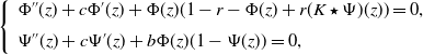 \begin{equation} \left \{ \begin{array}{cc} \begin{aligned} &\Phi ^{\prime\prime}(z)+c\Phi ^{\prime}(z)+\Phi (z)(1-r-\Phi (z)+r(K\star \Psi )(z))=0,\\[3pt] &\Psi ^{\prime\prime}(z)+c\Psi ^{\prime}(z)+b\Phi (z)(1-\Psi (z))=0,\\ \end{aligned} \end{array} \right . \end{equation}
where
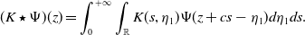 \begin{align*} (K\star \Psi )(z)= \int _{0}^{+\infty }\int _{\mathbb {R}}K(s,\eta _1)\Psi (z+cs-\eta _1)d\eta _1ds. \end{align*}
Here we have established a new coordinate-system $(\eta _1,\eta _2,\cdots, \eta _n)$
with
$(\eta _1,\eta _2,\cdots, \eta _n)$
with $\eta _1=\nu {\cdot}y$
and
$\eta _1=\nu {\cdot}y$
and
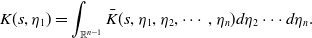 \begin{align*}K(s,\eta _1)= \int _{\mathbb {R}^{n-1}}\bar K(s,\eta _1,\eta _2,\cdots, \eta _n )d\eta _2 \cdots d\eta _n.\end{align*}
As such, the conditions (K1) and (K2) imply the following statements
-
1.
$\int _{0}^{\infty }\int _{\mathbb{R}} K(s,y)dyds=1$
, -
2. There exists
$\tilde{\delta }_0\in (0,\infty )$
such that
$\int _{0}^{\infty }\int _{\mathbb{R}} K(s,y)e^{\rho s}dyds\lt \infty$
for
$\rho \in [0, \tilde{\delta }_0)$


are true.
Since $(K\star \Psi )(z)$
depends on
$(K\star \Psi )(z)$
depends on $c$
, we may re-write it as
$c$
, we may re-write it as $(K\star _c\Psi )(z)$
to denote
$(K\star _c\Psi )(z)$
to denote $(K\star \Psi )(z)$
. The boundary condition of (1.5) at infinity is
$(K\star \Psi )(z)$
. The boundary condition of (1.5) at infinity is
 \begin{equation} (\Phi, \Psi )({-}\infty )=e_\beta \ \text{and} \ (\Phi, \Psi )(\infty )=e_0. \end{equation}
1.1. Bistable waves and the speed sign in the bistable case H1:
$ \boldsymbol{r} \gt 1$

Travelling waves are important phenomena and moved patterns in biological modelling and evolution. Following Murray’s initial works, many researchers delved into the study of system (1.1), with the problem of travelling waves emerging as a matter of fundamental interest. The primary focus of related research thus far has been on the localised case (e.g., [Reference Kanel16, Reference Murray28, Reference Murray29, Reference Troy33, Reference Ye and Wang43]), i.e. $(\bar{K}* v)(t, x)=v(t, x)$
, and the cases involving delays (e.g., [Reference Lin and Li19, Reference Trofimchuk, Pinto and Trofimchuk31, Reference Wu and Zou42, Reference Zhang44]),
$(\bar{K}* v)(t, x)=v(t, x)$
, and the cases involving delays (e.g., [Reference Lin and Li19, Reference Trofimchuk, Pinto and Trofimchuk31, Reference Wu and Zou42, Reference Zhang44]), $(\bar{K}* v)(t, x)=v(t-h, x)$
. However, there has been limited research of system (1.1) with non-local delayed interaction. Especially in the bistable case H1, (in fact,
$(\bar{K}* v)(t, x)=v(t-h, x)$
. However, there has been limited research of system (1.1) with non-local delayed interaction. Especially in the bistable case H1, (in fact, $r$
can vary between 5 and 50 in real experiments), a conjecture about the existence of bistable travelling wave was raised by Hasík et al. [Reference Hasík, Kopfová, Nábělková and Trofimchuk13]. To the best of our knowledge, no related contributions have been made for this, and in fact this problem has remained open for long time. In this article, we are able to solve the problem and will prove that there exists a unique (up to translation) bistable travelling wave of system (1.5)-(1.6), namely the following two theorems.
$r$
can vary between 5 and 50 in real experiments), a conjecture about the existence of bistable travelling wave was raised by Hasík et al. [Reference Hasík, Kopfová, Nábělková and Trofimchuk13]. To the best of our knowledge, no related contributions have been made for this, and in fact this problem has remained open for long time. In this article, we are able to solve the problem and will prove that there exists a unique (up to translation) bistable travelling wave of system (1.5)-(1.6), namely the following two theorems.
Theorem 1.1.
(Existence and the speed sign) Assume that H1 and (K1) hold. There exists a monotone bistable travelling wave $(c, \Phi (z), \Psi (z))$
,
$(c, \Phi (z), \Psi (z))$
, $z=\nu {\cdot}x-ct$
, for any given
$z=\nu {\cdot}x-ct$
, for any given $\nu$
with
$\nu$
with $||\nu ||=1$
, of system (1.5)-(1.6), where
$||\nu ||=1$
, of system (1.5)-(1.6), where $c$
is positive and unique. Moreover,
$c$
is positive and unique. Moreover, $\Phi ^{\prime}(z)\lt 0$
and
$\Phi ^{\prime}(z)\lt 0$
and $\Psi ^{\prime}(z)\lt 0$
for
$\Psi ^{\prime}(z)\lt 0$
for $z\in \mathbb{R}$
.
$z\in \mathbb{R}$
.
Theorem 1.2.
(Uniqueness) Assume that H1, (K1) and (K2) hold. If $(\Phi ^*(\nu\ {\cdot}\ x-c^*t),\Psi ^*(\nu\ {\cdot}\ x-c^*t))$
is a bistable travelling wave of system (1.2) connecting
$(\Phi ^*(\nu\ {\cdot}\ x-c^*t),\Psi ^*(\nu\ {\cdot}\ x-c^*t))$
is a bistable travelling wave of system (1.2) connecting $e_\beta$
to
$e_\beta$
to $e_0$
, then there exists
$e_0$
, then there exists $z^*\in \mathbb{R}$
such that
$z^*\in \mathbb{R}$
such that $(\Phi ^*(\nu\ {\cdot}\ x-c^*t),\Psi ^*(\nu\ {\cdot}\ x-c^*t))=(\Phi (\nu\ {\cdot}\ x-ct+z^*),\Psi (\nu\ {\cdot}\ x-ct+z^*))$
and
$(\Phi ^*(\nu\ {\cdot}\ x-c^*t),\Psi ^*(\nu\ {\cdot}\ x-c^*t))=(\Phi (\nu\ {\cdot}\ x-ct+z^*),\Psi (\nu\ {\cdot}\ x-ct+z^*))$
and $c^*=c$
, where
$c^*=c$
, where $(\Phi (\nu\ {\cdot}\ x-ct),\Psi (\nu\ {\cdot}\ x-ct))$
is the wave solution in Theorem 1.1. The bistable wave speed
$(\Phi (\nu\ {\cdot}\ x-ct),\Psi (\nu\ {\cdot}\ x-ct))$
is the wave solution in Theorem 1.1. The bistable wave speed $c$
is non-increasing in
$c$
is non-increasing in $r$
and is non-decreasing in
$r$
and is non-decreasing in $b$
.
$b$
.
The presence of continuum equilibria, combined with the non-local delayed reaction term, incorporates significant complexity when analysing model (1.1). This specific property of equilibrium $e_0$
hinders the application of Fang and Zhao’s abstract theory [Reference Fang and Zhao9] of bistable travelling waves for monotone semiflows to our system, as
$e_0$
hinders the application of Fang and Zhao’s abstract theory [Reference Fang and Zhao9] of bistable travelling waves for monotone semiflows to our system, as $e_0$
is not strongly stable in their settings, nor the intermediate equilibria are un-ordered. Furthermore, [Reference Fang and Zhao9] only consider a finite delay. Here, however, the delay in system (1.1) is infinitely distributed. Methods developed in other important studies (see, for example, [Reference Chen6, Reference Li and Zhang18]) remain unapplicable because they only allow a limited number of steady states. Kanel [Reference Kanel16] established the existence of the bistable travelling wave in the non-delayed local case (where
$e_0$
is not strongly stable in their settings, nor the intermediate equilibria are un-ordered. Furthermore, [Reference Fang and Zhao9] only consider a finite delay. Here, however, the delay in system (1.1) is infinitely distributed. Methods developed in other important studies (see, for example, [Reference Chen6, Reference Li and Zhang18]) remain unapplicable because they only allow a limited number of steady states. Kanel [Reference Kanel16] established the existence of the bistable travelling wave in the non-delayed local case (where $(\bar{K}* v)(t, x)=v(t, x)$
and
$(\bar{K}* v)(t, x)=v(t, x)$
and $r\gt 1$
) by using a shooting method in the phase plane. However, this method cannot be applied to non-local or delayed versions of system (1.1). Recently, Hasík et al. [Reference Hasík, Kopfová, Nábělková and Trofimchuk13] proved the existence of the bistable travelling wave in the delayed local case (where
$r\gt 1$
) by using a shooting method in the phase plane. However, this method cannot be applied to non-local or delayed versions of system (1.1). Recently, Hasík et al. [Reference Hasík, Kopfová, Nábělková and Trofimchuk13] proved the existence of the bistable travelling wave in the delayed local case (where $(\bar{K}* v)(t, x)=v(t-h, x)$
and
$(\bar{K}* v)(t, x)=v(t-h, x)$
and $r\gt 1$
) by constructing a perturbed system, which can approximate the original system. Application of the method in this article to the more complex system (1.1) with non-local delayed reaction is still in question, definitely in great challenge.
$r\gt 1$
) by constructing a perturbed system, which can approximate the original system. Application of the method in this article to the more complex system (1.1) with non-local delayed reaction is still in question, definitely in great challenge.
In order to address the challenges mentioned above, we shall develop novel approaches to rigourously show the existence of travelling wave solutions to the system exhibiting bistable nonlinearity. Our methodology utilises a combination of advanced analysis on partial differential equations (parabolic and elliptic) and dynamical techniques, enabling its application to nonlocal problems and high-dimensional phase systems. The novelty of our result is that we not only prove the existence, uniqueness and the positive speed sign of the bistable wave, but also provide the monotonicity of bistable wave speed $c$
with respect to parameters
$c$
with respect to parameters $r$
and
$r$
and $b$
. The bistable wave speed
$b$
. The bistable wave speed $c$
is non-increasing in
$c$
is non-increasing in $r$
and is non-decreasing in
$r$
and is non-decreasing in $b$
.
$b$
.
1.2. Monostable waves and speed selection in the case H2:
$ \boldsymbol{r} \le 1$

In the H2 case, the solution to (1.5)-(1.6) is usually not unique, as can be seen in the classical KPP–Fisher model [Reference Fisher10]. Denote $c_{\min }$
as
$c_{\min }$
as
 \begin{align*} c_{\min }=\inf \{c\ :\ (1.5)-(1.6) \ \text {has a non-negative solution}\}. \end{align*}
Standard linearisation near the equilibrium point $e_0$
shows
$e_0$
shows $c_{\min }\ge c_0=2\sqrt{1-r}$
. For convenience, we give the following definition on the minimal wave speed selection in the monostable case.
$c_{\min }\ge c_0=2\sqrt{1-r}$
. For convenience, we give the following definition on the minimal wave speed selection in the monostable case.
Definition 1.1.
If $c_{\min }=c_0$
, then we say the minimal wave speed is linearly selected and the wave is a pulled wave; If
$c_{\min }=c_0$
, then we say the minimal wave speed is linearly selected and the wave is a pulled wave; If $c_{\min }\gt c_0$
, then the minimal wave speed is said to be nonlinearly selected and the corresponding wave is a pushed wave.
$c_{\min }\gt c_0$
, then the minimal wave speed is said to be nonlinearly selected and the corresponding wave is a pushed wave.
Recently, Hasík et al. [Reference Hasík, Kopfová, Nábělková, Trofymchuk and Trofimchuk12] established the existence of monostable travelling wave of system (1.1) with spatio-temporal interaction for $r\in (0,1)$
and derived two limiting cases for the appearance of pushed wavefronts (nonlinear selection). These two sufficient conditions for nonlinear selection to system (1.1) in [Reference Hasík, Kopfová, Nábělková, Trofymchuk and Trofimchuk12] are as follows:
$r\in (0,1)$
and derived two limiting cases for the appearance of pushed wavefronts (nonlinear selection). These two sufficient conditions for nonlinear selection to system (1.1) in [Reference Hasík, Kopfová, Nábělková, Trofymchuk and Trofimchuk12] are as follows:
-
1) if
$b\rightarrow \infty$
, then
$c_{\min }\rightarrow 2$
; -
2) if the kernel function
$K(s,y)$
in (1.5) is replaced by
$K_a(s,y)=K(s,y+a)$
and
$a\rightarrow \infty$
, then
$c_{\min }\rightarrow 2$
.


In this article, we shall first give necessary and sufficient conditions for distinguishing between linear selection and nonlinear selection for all $r\le 1$
, including the existence of a family of travelling waves in the critical case
$r\le 1$
, including the existence of a family of travelling waves in the critical case $r=1$
whose dynamics behaves like the monostable case, instead of the bistable case, as shown in the following theorem.
$r=1$
whose dynamics behaves like the monostable case, instead of the bistable case, as shown in the following theorem.
Theorem 1.3. Assume that H2 and (K1) hold.
(i). There is a finite number $c_{\min }\ge c_0=2\sqrt{1-r}$
such that monotone and positive travelling wave solutions of (1.5)-(1.6) exist if and only if
$c_{\min }\ge c_0=2\sqrt{1-r}$
such that monotone and positive travelling wave solutions of (1.5)-(1.6) exist if and only if $c\ge c_{\min }$
. The minimal wave speed
$c\ge c_{\min }$
. The minimal wave speed $c_{\min }$
of (1.5)-(1.6) is nonlinearly selected if and only if there exists a wave front
$c_{\min }$
of (1.5)-(1.6) is nonlinearly selected if and only if there exists a wave front $(c_2, \Phi, \Psi ), c_2\gt c_0$
such that
$(c_2, \Phi, \Psi ), c_2\gt c_0$
such that
 \begin{align*}\Phi (z)\sim A_2e^{-\mu _2(c_2) z},\ \text {as} \ z\rightarrow \infty, \ z=\nu {\cdot}x-c_2t, \ ||\nu ||=1,\end{align*}
with $A_2\gt 0$
. Here,
$A_2\gt 0$
. Here, $\mu _2$
is the larger root of
$\mu _2$
is the larger root of $\mu ^2-c\mu +(1-r)=0$
. Furthermore,
$\mu ^2-c\mu +(1-r)=0$
. Furthermore, $c_2=c_{\min }$
.
$c_2=c_{\min }$
.
(ii) For $r\in (0,1)$
, the minimal speed
$r\in (0,1)$
, the minimal speed $c_{\min }$
is non-decreasing with respect to
$c_{\min }$
is non-decreasing with respect to $b$
. Then there exists a finite value
$b$
. Then there exists a finite value $b^*\gt 0$
such that
$b^*\gt 0$
such that $c_{\min }=c_0$
for
$c_{\min }=c_0$
for $b \in (0, b^*]$
, and
$b \in (0, b^*]$
, and $c_{\min }\in (c_0,2]$
for
$c_{\min }\in (c_0,2]$
for $b\gt b^*$
; If
$b\gt b^*$
; If $r=1$
, then
$r=1$
, then $c_{\min }\gt c_0$
for all positive parameter
$c_{\min }\gt c_0$
for all positive parameter $b$
.
$b$
.
(iii) For fixed $b$
, the minimal speed
$b$
, the minimal speed $c_{min}$
is a non-increasing function of
$c_{min}$
is a non-increasing function of $r$
in
$r$
in $(0,1]$
. Furthermore, there exists a unique turning point
$(0,1]$
. Furthermore, there exists a unique turning point $r^*\lt 1$
for the minimal speed selection, that is,
$r^*\lt 1$
for the minimal speed selection, that is, $c_{\min }=c_0$
for
$c_{\min }=c_0$
for $r \in (0, r^*]$
, and
$r \in (0, r^*]$
, and $c_{\min }\in (c_0,2]$
for
$c_{\min }\in (c_0,2]$
for $r\in (r^*, 1]$
.
$r\in (r^*, 1]$
.
Here, Theorem1.3 is a new development of the abstract results of speed selection in [Reference Ma and Ou23] to the system (1.1) with infinite points of equilibria. It shows that the minimal wave speed is non-decreasing with respect to $b$
, when
$b$
, when $r$
is fixed, and there exists a transition point, denoted as
$r$
is fixed, and there exists a transition point, denoted as $b^*$
, which serves as a turning point for speed selection. Similarly, there exists the monotonicity of the minimal wave speed with respect to
$b^*$
, which serves as a turning point for speed selection. Similarly, there exists the monotonicity of the minimal wave speed with respect to $r$
and the transition
$r$
and the transition $r^*$
for speed selection (when
$r^*$
for speed selection (when $b$
is fixed), although the linear speed varies with
$b$
is fixed), although the linear speed varies with $r$
.
$r$
.
Without any assumptions on the existence of wave fronts, we further provide the following easy-to-apply theorem, which can be used to derive a series of explicit conditions on speed selections by constructing various upper or lower solutions.
Theorem 1.4.
(Linear, nonlinear selection and estimate of $c_{\min }$
) Assume that H2 and (K1) hold.
$c_{\min }$
) Assume that H2 and (K1) hold. $\mu _1$
and
$\mu _1$
and $\mu _2 (\ge \mu _1)$
are two roots of
$\mu _2 (\ge \mu _1)$
are two roots of $\mu ^2-c\mu +(1-r)=0$
.
$\mu ^2-c\mu +(1-r)=0$
.
(i) For $c_1\gt c_0$
, if there exists a nonnegative and monotonic lower solution
$c_1\gt c_0$
, if there exists a nonnegative and monotonic lower solution $(\underline{\Phi },\underline{\Psi })(z)$
of system (1.5)-(1.6) such that
$(\underline{\Phi },\underline{\Psi })(z)$
of system (1.5)-(1.6) such that $\underline{\Phi }(z)\sim \underline{A} e^{-\mu _2 z}$
as
$\underline{\Phi }(z)\sim \underline{A} e^{-\mu _2 z}$
as $z\rightarrow \infty$
with
$z\rightarrow \infty$
with $\underline{A}\gt 0$
, and
$\underline{A}\gt 0$
, and $\limsup _{z\rightarrow -\infty }\underline{\Phi }(z)\lt 1$
, then no travelling wave solution exists for
$\limsup _{z\rightarrow -\infty }\underline{\Phi }(z)\lt 1$
, then no travelling wave solution exists for $c\in [c_0, c_1)$
and there exists
$c\in [c_0, c_1)$
and there exists $c_{\min }\gt c_1$
.
$c_{\min }\gt c_1$
.
(ii) For $r\in (0,1)$
and
$r\in (0,1)$
and $c=c_0+\varepsilon$
where
$c=c_0+\varepsilon$
where $\varepsilon$
is any small positive number, if there exists a nonnegative and monotonic upper solution
$\varepsilon$
is any small positive number, if there exists a nonnegative and monotonic upper solution $(\overline{\Phi },\overline{\Psi })(z)$
of system (1.5)-(1.6) such that
$(\overline{\Phi },\overline{\Psi })(z)$
of system (1.5)-(1.6) such that $\overline{\Phi }(z)\sim \overline{A} e^{-\mu _1(c) z}$
as
$\overline{\Phi }(z)\sim \overline{A} e^{-\mu _1(c) z}$
as $z\rightarrow \infty$
with
$z\rightarrow \infty$
with $\overline{A}\gt 0$
, and
$\overline{A}\gt 0$
, and $\limsup _{z\rightarrow -\infty }\overline{\Phi }(z)\ge 1$
, then we have
$\limsup _{z\rightarrow -\infty }\overline{\Phi }(z)\ge 1$
, then we have $c_{\min }=c_0$
.
$c_{\min }=c_0$
.
By application of this theorem, two explicit estimates about $b^*$
are given by applying Theorem1.4. The comparison of our new results to previous ones is given in the discussion section which shows the practicalness of this finding.
$b^*$
are given by applying Theorem1.4. The comparison of our new results to previous ones is given in the discussion section which shows the practicalness of this finding.
We also provide details of the decay rate of the minimal-speed travelling wave as $b$
varies around
$b$
varies around $b^*$
, which are substantially novel than our previous work [Reference Ma and Ou23]. These findings imply the transition wave behavies completely different from other pulled waves for
$b^*$
, which are substantially novel than our previous work [Reference Ma and Ou23]. These findings imply the transition wave behavies completely different from other pulled waves for $b\lt b^*$
, as shown in the following theorem.
$b\lt b^*$
, as shown in the following theorem.
Theorem 1.5.
Assume that H2 and (K1) hold. Let $b^*$
be the turning point for the minimal speed selection for fixed
$b^*$
be the turning point for the minimal speed selection for fixed $r$
, specifically
$r$
, specifically $c_{\min }=c_0$
for
$c_{\min }=c_0$
for $b \in (0, b^*]$
, and
$b \in (0, b^*]$
, and $c_{\min }\in (c_0,2]$
for
$c_{\min }\in (c_0,2]$
for $b\gt b^*$
. The behaviour of the minimal-speed travelling wave solution
$b\gt b^*$
. The behaviour of the minimal-speed travelling wave solution $(\Phi (z), \Psi (z))$
of system (1.5)-(1.6) can be described as follows:
$(\Phi (z), \Psi (z))$
of system (1.5)-(1.6) can be described as follows:
-
(1) if
$b\in (0, b^*)$
, then
$\Phi (z)\sim Aze^{-\mu _1(c_0) z}$
as
$z\rightarrow \infty$
, where
$A\gt 0$
; -
(2) if
$b=b^*$
, then
$\Phi (z)\sim Be^{-\mu _1(c_0) z}$
as
$z\rightarrow \infty$
, where
$B\gt 0$
; -
(3) if
$b\gt b^*$
, then
$\Phi (z)\sim Be^{-\mu _2(c_{\min }) z}$
as
$z\rightarrow \infty$
, where
$B\gt 0$
.


Here, $\mu _1$
and
$\mu _1$
and $\mu _2 (\ge \mu _1)$
are two roots of
$\mu _2 (\ge \mu _1)$
are two roots of $\mu ^2-c\mu +(1-r)=0$
.
$\mu ^2-c\mu +(1-r)=0$
.
Remark 1.1. The above Theorem 1.1 corresponds to Theorem 2.6 , Theorem 1.2 corresponds to Theorems 2.8 - 2.9 , Theorem 1.3 corresponds to Theorems 3.3 , 3.4 , 3.6 and 3.10 , Theorem 1.4 corresponds to Theorem 3.5 , and Theorem 1.5 corresponds to Theorem 3.9 .
Finally, we would like to provide readers with a few more references related to our study. In recent years, considerable efforts have been made in studying the existence of travelling waves and their speed sign for monotonic systems. See e.g., [Reference Alhasanat and Ou2, Reference Aronson and Weinberger4, Reference Bates, Chen and Chmaj5, Reference Fang and Zhao8 Reference Fang and Zhao9 Reference Fisher10, Reference Ma, Huang and Ou22, Reference Ma, Yue and Ou24, Reference Ma and Ou26, Reference Ma, Zhang, Yue and Ou27, Reference Volpert, Volpert and Volpert34, Reference Wang and Ou36, Reference Wang and Ou37, Reference Wang, Wang and Ou39]. The problem of the minimal speed selection was widely discussed in many papers. See, e.g., [Reference Alhasanat and Ou1, Reference Alhasanat and Ou3, Reference Aronson and Weinberger4, Reference Huang and Ou14, Reference Huang and Ou15, Reference Liu, Ouyang, Huang and Ou20, Reference Lucia, Muratov and Novaga21, Reference Ma and Ou23, Reference Ma and Ou25, Reference Pan, Wang and Ou30, Reference Wang, Huang and Ou35, Reference Weinberger, Lewis and Li40, Reference Wu, Xiao and Zhou41].
The remainder of this paper is organised as follows. In Section 2, we prove the existence and uniqueness of the monotone bistable travelling wave of (1.5)-(1.6) for the case H1. In Section 3, we prove the existence of monostable travelling wave of (1.5)-(1.6) for $r=1$
. We also derive necessary and sufficient conditions for speed selection and give the decay rate of the minimal-speed travelling wave as
$r=1$
. We also derive necessary and sufficient conditions for speed selection and give the decay rate of the minimal-speed travelling wave as $z\rightarrow \infty$
, in terms of different value domains of
$z\rightarrow \infty$
, in terms of different value domains of $b$
around of
$b$
around of $b^*$
, under the case H2. Section 4 will present numerical results, while Section 5 covers the conclusion and the further discussion.
$b^*$
, under the case H2. Section 4 will present numerical results, while Section 5 covers the conclusion and the further discussion.
2. Bistable wave in the case H1: existence, uniqueness and speed sign
In this section, we consider system (1.2) under the condition H1. Note that $e_\beta$
is stable, and
$e_\beta$
is stable, and $e_0$
is non-asymptotically stable nor strongly stable. As mentioned in Section 1, the use of the monotonic semiflow theory in [Reference Fang and Zhao9] is not applicable for proving the existence of the bistable monotone travelling wave solution in (1.5)-(1.6). The non-local delayed reaction term in system (1.5) prevents the utilisation of the shooting method. Here, we present a novel approach to establish the existence of wavefront, which could potentially be extended to other models featuring non-isolated equilibrium points and non-local delayed reaction terms.
$e_0$
is non-asymptotically stable nor strongly stable. As mentioned in Section 1, the use of the monotonic semiflow theory in [Reference Fang and Zhao9] is not applicable for proving the existence of the bistable monotone travelling wave solution in (1.5)-(1.6). The non-local delayed reaction term in system (1.5) prevents the utilisation of the shooting method. Here, we present a novel approach to establish the existence of wavefront, which could potentially be extended to other models featuring non-isolated equilibrium points and non-local delayed reaction terms.
Obviously, it can be seen from the second equation of (1.5) that this model has no positive and monotone travelling wave satisfying (1.6) with speed $c\le 0$
. The following lemma gives the existence of solutions to the
$c\le 0$
. The following lemma gives the existence of solutions to the $\Psi$
-equation of the system (1.5)-(1.6) when
$\Psi$
-equation of the system (1.5)-(1.6) when $\Phi$
is given, which holds for both bistable and monostable cases.
$\Phi$
is given, which holds for both bistable and monostable cases.
Lemma 2.1.
Let $c\gt 0$
and
$c\gt 0$
and $b\gt 0$
, and suppose that
$b\gt 0$
, and suppose that $\Phi (z)$
is a positive non-increasing continuous function such that
$\Phi (z)$
is a positive non-increasing continuous function such that $\Phi ({-}\infty )=1$
and
$\Phi ({-}\infty )=1$
and $\int _{0}^{\infty } \Phi (z)dz$
is finite. Then there exists a unique monotone
$\int _{0}^{\infty } \Phi (z)dz$
is finite. Then there exists a unique monotone $C^2$
-smooth solution
$C^2$
-smooth solution $\Psi (z)$
,
$\Psi (z)$
, $\Psi ^{\prime}(z)\lt 0$
, to the boundary value problem
$\Psi ^{\prime}(z)\lt 0$
, to the boundary value problem
 \begin{equation} \Psi ^{\prime\prime}(z)+c\Psi ^{\prime}(z)+b\Phi (z)(1-\Psi (z))=0, \quad \Psi ({-}\infty )=1, \quad \Psi (\infty )=0. \end{equation}
This defines the operator $\mathcal{L}_{b,c}$
, by
$\mathcal{L}_{b,c}$
, by $\Psi =\mathcal{L}_{b,c}\Phi$
on the respective functional sets.
$\Psi =\mathcal{L}_{b,c}\Phi$
on the respective functional sets. $\mathcal{L}_{b,c}$
commutes with the translation operator,
$\mathcal{L}_{b,c}$
commutes with the translation operator, $(\mathcal{L}_{b,c}\Phi ({\cdot}+h))(z)=(\mathcal{L}_{b,c}\Phi ({\cdot}))(z+h)$
, and is monotonic with respect to
$(\mathcal{L}_{b,c}\Phi ({\cdot}+h))(z)=(\mathcal{L}_{b,c}\Phi ({\cdot}))(z+h)$
, and is monotonic with respect to $b$
,
$b$
, $c$
and
$c$
and $\Phi$
so that
$\Phi$
so that
-
(a) if
$\Phi _1(z)\le \Phi _2(z)$
, then
$(\mathcal{L}_{b,c}(\Phi _1))(z)\le (\mathcal{L}_{b,c}(\Phi _2))(z)$
,
$z\in \mathbb{R}$
; -
(b) if
$b_1\lt b_2$
, then
$(\mathcal{L}_{b_1,c}(\Phi ))(z)\lt (\mathcal{L}_{b_2,c}(\Phi ))(z)$
,
$z\in \mathbb{R}$
, for each
$\Phi$
from the domain of
$\mathcal{L}_{b,c}$
. Moreover, we have
$\mathcal{L}_{b,c}\Phi \rightarrow 0$
as
$b\rightarrow 0$
, and
$\mathcal{L}_{b,c}\Phi \rightarrow 1$
as
$b\rightarrow \infty$
; -
(c) if
$c_1\lt c_2$
, then
$(\mathcal{L}_{b,c_1}(\Phi ))(z)\gt (\mathcal{L}_{b,c_2}(\Phi ))(z)$
,
$z\in \mathbb{R}$
, for each
$\Phi$
from the domain of
$\mathcal{L}_{b,c}$
. Moreover, we have
$\mathcal{L}_{b,c}\Phi \rightarrow 1$
as
$c\rightarrow 0$
.


Proof. We only prove result $c)$
and the limiting results in
$c)$
and the limiting results in $b)$
. The remaining parts can refer to [Reference Hasík, Kopfová, Nábělková, Trofymchuk and Trofimchuk12, Lemma 15]. We let
$b)$
. The remaining parts can refer to [Reference Hasík, Kopfová, Nábělková, Trofymchuk and Trofimchuk12, Lemma 15]. We let $c_1\lt c_2$
, and set
$c_1\lt c_2$
, and set $\Psi _j=\mathcal{L}_{b,c_j}\Phi$
,
$\Psi _j=\mathcal{L}_{b,c_j}\Phi$
, $j=1,2$
. Take
$j=1,2$
. Take $\sigma (z)=\Psi _1(z)-\Psi _2(z)$
,
$\sigma (z)=\Psi _1(z)-\Psi _2(z)$
, $z\in \mathbb{R}$
. Then
$z\in \mathbb{R}$
. Then $\sigma (z)$
satisfies
$\sigma (z)$
satisfies
 \begin{align*} \sigma ^{\prime\prime}(z)+c_1\sigma ^{\prime}(z)+(c_1-c_2)\Psi _2^{\prime}(z)-b\Phi (z)\sigma (z)=0, \quad \sigma ({-}\infty )=0, \quad \sigma (\infty )=0. \end{align*}
If $\sigma (s)\le 0$
at some point
$\sigma (s)\le 0$
at some point $s$
, then there exists a critical point
$s$
, then there exists a critical point $s^*$
such that
$s^*$
such that $\sigma (s^*)\le 0$
,
$\sigma (s^*)\le 0$
, $\sigma ^{\prime}(s^*)=0$
, and
$\sigma ^{\prime}(s^*)=0$
, and $\sigma ^{\prime\prime}(s^*)\ge 0$
. It follows that
$\sigma ^{\prime\prime}(s^*)\ge 0$
. It follows that
 \begin{align*} \sigma ^{\prime\prime}(s^*)+c_1\sigma ^{\prime}(s^*)+(c_1-c_2)\Psi _2^{\prime}(s^*)-b\Phi (s^*)\sigma (s^*)\gt 0 \end{align*}
since $\Psi _2^{\prime}(s^*)\lt 0$
. It is a contradiction. Therefore,
$\Psi _2^{\prime}(s^*)\lt 0$
. It is a contradiction. Therefore, $\Psi _1(z)\ge \Psi _2(z)$
,
$\Psi _1(z)\ge \Psi _2(z)$
, $z\in \mathbb{R}$
.
$z\in \mathbb{R}$
.
To prove $\mathcal{L}_{b,c}\Phi \rightarrow 1$
as
$\mathcal{L}_{b,c}\Phi \rightarrow 1$
as $c\rightarrow 0$
, we consider a decreasing sequence
$c\rightarrow 0$
, we consider a decreasing sequence $c_n=\frac{1}{n}$
,
$c_n=\frac{1}{n}$
, $n\in \mathbb{N}^+$
. Then by the monotonicity of
$n\in \mathbb{N}^+$
. Then by the monotonicity of $\mathcal{L}_{b,c}\Phi$
with respect to
$\mathcal{L}_{b,c}\Phi$
with respect to $c$
, we know
$c$
, we know $\Psi ^n(z)\,:\!=\,\mathcal{L}_{b,c_n}\Phi (z)$
is increasing with respect to
$\Psi ^n(z)\,:\!=\,\mathcal{L}_{b,c_n}\Phi (z)$
is increasing with respect to $n$
. Note that
$n$
. Note that $1$
is an upper bound of the sequence
$1$
is an upper bound of the sequence $\Psi ^n(z)$
, and
$\Psi ^n(z)$
, and $1$
is the only positive and non-increasing solution to the following problem
$1$
is the only positive and non-increasing solution to the following problem
 \begin{align*} \Psi ^{\prime\prime}(z)+b\Phi (z)(1-\Psi (z))=0, \quad \Psi ({-}\infty )=1.\end{align*}
Thus, we have $\Psi ^n(z)\rightarrow 1$
as
$\Psi ^n(z)\rightarrow 1$
as $n\rightarrow \infty$
, that is,
$n\rightarrow \infty$
, that is, $\Psi =\mathcal{L}_{b,c}\Phi \rightarrow 1$
as
$\Psi =\mathcal{L}_{b,c}\Phi \rightarrow 1$
as $c\rightarrow 0$
.
$c\rightarrow 0$
.
By the similar arguments to the proof of $\mathcal{L}_{b,c}\Phi \rightarrow 1$
as
$\mathcal{L}_{b,c}\Phi \rightarrow 1$
as $c\rightarrow 0$
and the monotonicity of
$c\rightarrow 0$
and the monotonicity of $\mathcal{L}_{b,c}\Phi$
with respect to
$\mathcal{L}_{b,c}\Phi$
with respect to $b$
(refer to [Reference Hasík, Kopfová, Nábělková, Trofymchuk and Trofimchuk12, Lemma 15]), we can derive
$b$
(refer to [Reference Hasík, Kopfová, Nábělková, Trofymchuk and Trofimchuk12, Lemma 15]), we can derive $\mathcal{L}_{b,c}\Phi \rightarrow 0$
as
$\mathcal{L}_{b,c}\Phi \rightarrow 0$
as $b\rightarrow 0$
and
$b\rightarrow 0$
and $\mathcal{L}_{b,c}\Phi \rightarrow 1$
as
$\mathcal{L}_{b,c}\Phi \rightarrow 1$
as $b\rightarrow \infty$
.
$b\rightarrow \infty$
.
2.1. Bistable waves of an auxiliary equation
In this subsection, we shall prove the existence of the bistable travelling wave of an auxiliary equation we derive. According to Lemma 2.1, system (1.5)-(1.6) can be transformed into the following equation
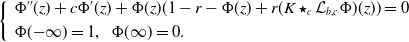 \begin{equation} \left \{ \begin{array}{cc} \begin{aligned} &\Phi ^{\prime\prime}(z)+c\Phi ^{\prime}(z)+\Phi (z)(1-r-\Phi (z)+r(K\star _c\mathcal{L}_{b,c}\Phi )(z))=0 \\ &\Phi ({-}\infty )=1,\ \ \Phi (\infty )=0. \end{aligned} \end{array}\right . \end{equation}
Consider the wave speed $c\gt 0$
in
$c\gt 0$
in $\mathcal{L}_{b,c}\Phi$
of (2.2) as a parameter. We would like to construct an auxiliary parabolic partial differential equation as follows
$\mathcal{L}_{b,c}\Phi$
of (2.2) as a parameter. We would like to construct an auxiliary parabolic partial differential equation as follows
 \begin{equation} \phi _t(t,x)=\phi _{xx}(t,x)+\phi (t,x)(1-r-\phi (t,x)+r(K*\mathcal{L}_{b,c}\phi )(t,x)),\ x\in \mathbb{R}. \end{equation}
Clearly, (2.3) has two constant equilibria $\phi =0$
and
$\phi =0$
and $\phi =1$
. Due to the condition that
$\phi =1$
. Due to the condition that $\int _{0}^{\infty } \Phi (z)dz$
is finite in Lemma 2.1, the initial function for (2.3) needs to be restricted as integrable at
$\int _{0}^{\infty } \Phi (z)dz$
is finite in Lemma 2.1, the initial function for (2.3) needs to be restricted as integrable at $\infty$
. Since the model is monotone, the well-posedness of this problem has no problem and the solution still belongs to be integrable at
$\infty$
. Since the model is monotone, the well-posedness of this problem has no problem and the solution still belongs to be integrable at $\infty$
for any future time
$\infty$
for any future time $t$
. To investigate the travelling wave to (2.3), we define
$t$
. To investigate the travelling wave to (2.3), we define
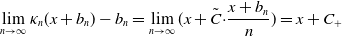
 \begin{align*} \phi (t,x)=\Phi (z), \ \ z= x-C(c)t, \end{align*}
where $C(c)$
represents the wave speed dependent on
$C(c)$
represents the wave speed dependent on $c$
. Substituting this into (2.3), we obtain
$c$
. Substituting this into (2.3), we obtain
 \begin{equation} \Phi ^{\prime\prime}(z)+C(c)\Phi ^{\prime}(z)+\Phi (z)(1-r-\Phi (z)+r(K\star _{C(c)}\mathcal{L}_{b,c}\Phi )(z))=0 \end{equation}
subject to the boundary conditions
 \begin{equation} \Phi ({-}\infty )=1,\ \ \ \Phi (\infty )=0. \end{equation}
We aim to prove the existence of wavefront $(C(c), \Phi )$
, with
$(C(c), \Phi )$
, with $C(c)$
being non-increasing function of
$C(c)$
being non-increasing function of $c$
.
$c$
.
Let $X=BC(\mathbb{R}, \mathbb{R})$
be the space of all bounded, continuous and integrable-at-positive-
$X=BC(\mathbb{R}, \mathbb{R})$
be the space of all bounded, continuous and integrable-at-positive- $\infty$
functions from
$\infty$
functions from $\mathbb{R}$
to
$\mathbb{R}$
to $\mathbb{R}$
. Define
$\mathbb{R}$
. Define $X_+=\{ \varphi \in X\ :\ \varphi (x) \geq 0, \forall x\in \mathbb{R} \}$
. Let
$X_+=\{ \varphi \in X\ :\ \varphi (x) \geq 0, \forall x\in \mathbb{R} \}$
. Let $\mathcal{C}=C(M,X)$
be the space of all functions from
$\mathcal{C}=C(M,X)$
be the space of all functions from $M$
to
$M$
to $X$
with
$X$
with $|{\cdot}|_{\mathcal{C}}=||{\cdot}||_\infty$
, where
$|{\cdot}|_{\mathcal{C}}=||{\cdot}||_\infty$
, where $M=({-}\infty, 0]$
. Let
$M=({-}\infty, 0]$
. Let $\mathcal{C}_+=C(M,X_+)$
. Define
$\mathcal{C}_+=C(M,X_+)$
. Define $\mathcal{M}\subset \mathcal{C}$
to be the set of all continuous and non-increasing functions.
$\mathcal{M}\subset \mathcal{C}$
to be the set of all continuous and non-increasing functions. $\mathcal{M}_\beta =\{\varphi \in \mathcal{C}\ :\ 0\leq \varphi \leq \beta \}$
, where
$\mathcal{M}_\beta =\{\varphi \in \mathcal{C}\ :\ 0\leq \varphi \leq \beta \}$
, where $\beta =\textbf{1}$
in
$\beta =\textbf{1}$
in $\mathcal{C}$
.
$\mathcal{C}$
.
Denote $\{Q_t\}_{t\ge 0}$
as the solution semiflow associated with (2.3) on
$\{Q_t\}_{t\ge 0}$
as the solution semiflow associated with (2.3) on $\mathcal{C}_+$
. That is,
$\mathcal{C}_+$
. That is,
 \begin{align*} Q_t[\varphi ](\theta, x)=\phi (t+\theta, x,\varphi ), \ \forall \varphi \in \mathcal {C}, \ x\in \mathbb {R}, \ t\ge 0, \end{align*}
where $\phi (t+\theta, x,\varphi )$
is the unique solution of (2.3) satisfying
$\phi (t+\theta, x,\varphi )$
is the unique solution of (2.3) satisfying $\phi (\theta, {\cdot},\varphi )=\varphi (\theta )$
. Let
$\phi (\theta, {\cdot},\varphi )=\varphi (\theta )$
. Let $E$
be the set of all fixed points of
$E$
be the set of all fixed points of $Q_t$
for
$Q_t$
for $t\gt 0$
restricted to
$t\gt 0$
restricted to $\mathbb{R}$
. Then
$\mathbb{R}$
. Then $E=\{0, \beta \}$
. We use
$E=\{0, \beta \}$
. We use $Q$
to denote
$Q$
to denote $Q_1$
, and
$Q_1$
, and $Q^n$
is the
$Q^n$
is the $n$
-th iteration of
$n$
-th iteration of $Q$
.
$Q$
.
For $\theta \in M$
, we assume that
$\theta \in M$
, we assume that $\underline{\phi }$
and
$\underline{\phi }$
and $\bar{\phi }$
are non-increasing functions in
$\bar{\phi }$
are non-increasing functions in $\mathcal{M}_\beta$
satisfying
$\mathcal{M}_\beta$
satisfying
 \begin{equation} \underline{\phi }(\theta, z)=\underline{\phi }(z)=\left \{ \begin{aligned}&(1-\tilde{\delta })(1-e^{\tilde{\mu } z}), & z\lt 0,\\ &0, &z\ge 0,\\ \end{aligned}\right . \quad \bar{\phi }(\theta, z)=\bar{\phi }(z)=\left \{ \begin{aligned}&1, & z\le 0,\\ &e^{-\sqrt{r-1}z}, &z\gt 0, \end{aligned}\right . \end{equation}
where $\tilde{\delta }\gt 0$
is small, and
$\tilde{\delta }\gt 0$
is small, and $\tilde{\mu }$
is a positive constant. Clearly,
$\tilde{\mu }$
is a positive constant. Clearly, $\underline{\phi }\le \bar{\phi }$
.
$\underline{\phi }\le \bar{\phi }$
.
Lemma 2.2.
Assume that H1 and (K1) hold. There exist positive numbers $\tilde{C}\gt 0$
and
$\tilde{C}\gt 0$
and $\tilde{\mu }\gt 0$
such that for any
$\tilde{\mu }\gt 0$
such that for any $C\ge \tilde{C}$
, we have
$C\ge \tilde{C}$
, we have
 \begin{equation} Q[\underline{\phi }](\theta, x)\ge \underline{\phi }(\theta, x+C) \ \ \text{and} \ \ Q[\bar{\phi }](\theta, x)\le \bar{\phi }(\theta, x-C) \ \text{for all} \ x\in \mathbb{R}. \end{equation}
Proof. Let $\tilde{z}_1= x-Ct$
. When
$\tilde{z}_1= x-Ct$
. When $\tilde{z}_1\le 0$
, we have
$\tilde{z}_1\le 0$
, we have $\bar{\phi }(\tilde{z}_1)=1$
, and then
$\bar{\phi }(\tilde{z}_1)=1$
, and then
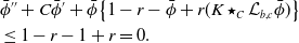 \begin{equation} \begin{aligned} &\bar{\phi }^{\prime\prime}+C\bar{\phi }^{\prime}+\bar{\phi }\big \{1-r-\bar{\phi }+r(K\star _C\mathcal{L}_{b,c}\bar{\phi })\big \}\\ &\le 1-r-1+r=0. \end{aligned} \end{equation}
When $\tilde{z}_1\gt 0$
, we obtain
$\tilde{z}_1\gt 0$
, we obtain $\bar{\phi }(\tilde{z}_1)=e^{-\sqrt{r-1} \tilde{z}_1}$
. For any
$\bar{\phi }(\tilde{z}_1)=e^{-\sqrt{r-1} \tilde{z}_1}$
. For any $C\ge \tilde{C}_1$
, where
$C\ge \tilde{C}_1$
, where $\tilde{C}_1$
satisfies
$\tilde{C}_1$
satisfies $-\sqrt{r-1}\tilde{C}_1+r=0$
, it gives
$-\sqrt{r-1}\tilde{C}_1+r=0$
, it gives
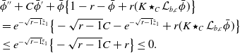 \begin{equation} \begin{aligned} &\bar{\phi }^{\prime\prime}+C\bar{\phi }^{\prime}+\bar{\phi }\big \{1-r-\bar{\phi }+r(K\star _C\mathcal{L}_{b,c}\bar{\phi })\big \}\\ &=e^{-\sqrt{r-1} \tilde{z}_1}\big \{-\sqrt{r-1} C-e^{-\sqrt{r-1} \tilde{z}_1}+r(K\star _C\mathcal{L}_{b,c}\bar{\phi })\big \}\\ &\le e^{-\sqrt{r-1} \tilde{z}_1}\big \{-\sqrt{r-1} C+r\big \} \le 0. \end{aligned} \end{equation}
Hence, we conclude that $Q[\bar{\phi }](\theta, x)\le \bar{\phi }(\theta, x-C)$
. In order to prove
$Q[\bar{\phi }](\theta, x)\le \bar{\phi }(\theta, x-C)$
. In order to prove $Q[\underline{\phi }](\theta, x)\ge \underline{\phi }(\theta, x+C)$
, we let
$Q[\underline{\phi }](\theta, x)\ge \underline{\phi }(\theta, x+C)$
, we let $\tilde{z}_2= x+Ct$
. Choose sufficiently small
$\tilde{z}_2= x+Ct$
. Choose sufficiently small $\tilde{\epsilon }\gt 0$
and
$\tilde{\epsilon }\gt 0$
and $\tilde{\epsilon }_1\gt 0$
such that
$\tilde{\epsilon }_1\gt 0$
such that
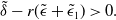 \begin{equation} \tilde{\delta }-r(\tilde{\epsilon }+\tilde{\epsilon }_1)\gt 0. \end{equation}
Since $\int _{0}^{\infty }\int _{\mathbb{R}}K(s,y)dyds=1$
, there exist a large enough
$\int _{0}^{\infty }\int _{\mathbb{R}}K(s,y)dyds=1$
, there exist a large enough $\tilde{M}_1\gt 0$
such that
$\tilde{M}_1\gt 0$
such that
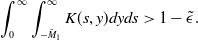 \begin{equation} \int _{0}^{\infty }\int _{-\tilde{M}_1}^\infty K(s,y)dyds\gt 1-\tilde{\epsilon }. \end{equation}
Note that we can still derive the existence of $\Psi$
in (2.1) when we choose
$\Psi$
in (2.1) when we choose $\Phi (z)=\underline{\phi }(z)$
(Here,
$\Phi (z)=\underline{\phi }(z)$
(Here, $\Phi ({-}\infty )=1-\tilde{\delta }$
). There exists
$\Phi ({-}\infty )=1-\tilde{\delta }$
). There exists $M_0(c)\lt 0$
so that
$M_0(c)\lt 0$
so that
 \begin{equation} \mathcal{L}_{b,c}\underline{\phi }(\tilde{z}_2)\gt 1-\tilde{\epsilon }_1 \quad \text{when} \ \tilde{z}_2\lt M_0(c). \end{equation}
For $\tilde{z}_2\lt M_0(c)-\tilde{M}_1\lt 0$
, if
$\tilde{z}_2\lt M_0(c)-\tilde{M}_1\lt 0$
, if $C\ge \tilde{\mu }$
, then by (2.10), (2.11) and (2.12), we have
$C\ge \tilde{\mu }$
, then by (2.10), (2.11) and (2.12), we have
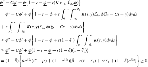 \begin{equation} \begin{aligned} &\underline{\phi }^{\prime\prime}-C\underline{\phi }^{\prime}+\underline{\phi }\big \{1-r-\underline{\phi }+r(K\star _{-C}\mathcal{L}_{b,c}\underline{\phi })\big \}\\ &=\underline{\phi }^{\prime\prime}-C\underline{\phi }^{\prime}+\underline{\phi }\bigg \{1-r-\underline{\phi }+r\int _{0}^{\infty }\int _{-\infty }^{-\tilde{M}_1}K(s,y)\mathcal{L}_{b,c}\underline{\phi }(\tilde{z}_2-Cs-y)dyds\\ &+r\int _{0}^{\infty }\int _{-\tilde{M}_1}^{\infty }K(s,y)\mathcal{L}_{b,c}\underline{\phi }(\tilde{z}_2-Cs-y)dyds \bigg \} \\ &\ge \underline{\phi }^{\prime\prime}-C\underline{\phi }^{\prime}+\underline{\phi }\bigg \{1-r-\underline{\phi }+r(1-\tilde{\epsilon }_1)\int _{0}^{\infty }\int _{-\tilde{M}_1}^{\infty }K(s,y)dyds \bigg \}\\ &\ge \underline{\phi }^{\prime\prime}-C\underline{\phi }^{\prime}+\underline{\phi }\{1-r-\underline{\phi }+r(1-\tilde{\epsilon })(1-\tilde{\epsilon }_1)\}\\ &=(1-\tilde{\delta })\bigg \{ \tilde{\mu }e^{\tilde{\mu } \tilde{z}_2} (C-\tilde{\mu }) +(1-e^{\tilde{\mu } \tilde{z}_2})[\tilde{\delta }-r(\tilde{\epsilon }+\tilde{\epsilon }_1) +r\tilde{\epsilon }\tilde{\epsilon }_1+(1-\tilde{\delta })e^{\tilde{\mu } \tilde{z}_2}] \bigg \}\ge 0.\\ \end{aligned} \end{equation}
Take $\tilde{\eta }\,:\!=\,\frac{\underline{\phi }(M_0(c)-\tilde{M}_1)}{1-\tilde{\delta }}\in (0,1)$
. For
$\tilde{\eta }\,:\!=\,\frac{\underline{\phi }(M_0(c)-\tilde{M}_1)}{1-\tilde{\delta }}\in (0,1)$
. For $\tilde{z}_2\in [M_0(c)-\tilde{M}_1,0)$
, we have
$\tilde{z}_2\in [M_0(c)-\tilde{M}_1,0)$
, we have $\underline{\phi }(\tilde{z}_2)\in (0, \tilde{\eta }(1-\tilde{\delta })]$
and
$\underline{\phi }(\tilde{z}_2)\in (0, \tilde{\eta }(1-\tilde{\delta })]$
and $e^{\tilde{\mu } \tilde{z}_2}\in [1-\tilde{\eta },1)$
. If
$e^{\tilde{\mu } \tilde{z}_2}\in [1-\tilde{\eta },1)$
. If $C\ge \frac{\tilde{\mu }^2+\tilde{\eta }[\tilde{\eta }(1-\tilde{\delta })+r-1]}{\tilde{\mu }(1-\tilde{\eta })}$
, then
$C\ge \frac{\tilde{\mu }^2+\tilde{\eta }[\tilde{\eta }(1-\tilde{\delta })+r-1]}{\tilde{\mu }(1-\tilde{\eta })}$
, then
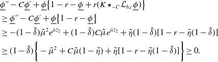 \begin{equation} \begin{aligned} &\underline{\phi }^{\prime\prime}-C\underline{\phi }^{\prime}+\underline{\phi }\big \{1-r-\underline{\phi }+r(K\star _{-C}\mathcal{L}_{b,c}\underline{\phi })\big \}\\ &\ge \underline{\phi }^{\prime\prime}-C\underline{\phi }^{\prime}+\underline{\phi }\big \{1-r-\underline{\phi }\big \}\\ &\ge -(1-\tilde{\delta })\tilde{\mu }^2e^{\tilde{\mu } \tilde{z}_2}+(1-\tilde{\delta })C\tilde{\mu }e^{\tilde{\mu } \tilde{z}_2}+\tilde{\eta }(1-\tilde{\delta })[1-r-\tilde{\eta }(1-\tilde{\delta })]\\ &\ge (1-\tilde{\delta })\bigg \{ -\tilde{\mu }^2+C\tilde{\mu }(1-\tilde{\eta })+\tilde{\eta }[1-r-\tilde{\eta }(1-\tilde{\delta })] \bigg \}\ge 0.\\ \end{aligned} \end{equation}
For $\tilde{z}_2\ge 0$
, we have
$\tilde{z}_2\ge 0$
, we have $\underline{\phi }(\tilde{z}_2)=0$
, and thus
$\underline{\phi }(\tilde{z}_2)=0$
, and thus
 \begin{equation} \underline{\phi }^{\prime\prime}-C\underline{\phi }^{\prime}+\underline{\phi }\big \{1-r-\underline{\phi }+r(K\star _{-C}\mathcal{L}_{b,c}\underline{\phi })\big \}=0. \end{equation}
Therefore, $Q[\underline{\phi }](\theta, x)\ge \underline{\phi }(\theta, x+C)$
for all
$Q[\underline{\phi }](\theta, x)\ge \underline{\phi }(\theta, x+C)$
for all $C\ge \tilde{C}_2\,:\!=\,\max \{\frac{\tilde{\mu }^2+\tilde{\eta }[\tilde{\eta }(1-\tilde{\delta })+r-1]}{\tilde{\mu }(1-\tilde{\eta })}, \tilde{\mu } \}$
. Let
$C\ge \tilde{C}_2\,:\!=\,\max \{\frac{\tilde{\mu }^2+\tilde{\eta }[\tilde{\eta }(1-\tilde{\delta })+r-1]}{\tilde{\mu }(1-\tilde{\eta })}, \tilde{\mu } \}$
. Let $\tilde{C}=\max \{\tilde{C}_1, \tilde{C}_2\}$
. Thus, the proof is complete.
$\tilde{C}=\max \{\tilde{C}_1, \tilde{C}_2\}$
. Thus, the proof is complete.
According to this lemma, when $C$
is large, the functions
$C$
is large, the functions $ \bar{\phi }(\theta, x-Ct)$
and
$ \bar{\phi }(\theta, x-Ct)$
and $\underline{\phi }(\theta, x+Ct)$
serve as upper and lower solutions, respectively, to the auxiliary equation (2.3). For each value of
$\underline{\phi }(\theta, x+Ct)$
serve as upper and lower solutions, respectively, to the auxiliary equation (2.3). For each value of $n$
, a shift is applied to both the upper and lower solutions, resulting in the definitions of
$n$
, a shift is applied to both the upper and lower solutions, resulting in the definitions of
 \begin{align*} \underline {\phi }_n(\theta, x)=\underline {\phi }(\theta, x+n+\tilde {C}) \quad \text {and} \quad \bar {\phi }_n(\theta, x)=\bar {\phi }(\theta, x-(n+\tilde {C})). \end{align*}
It is evident that due to the translation invariance property, both $\underline{\phi }_n(\theta, x)$
and
$\underline{\phi }_n(\theta, x)$
and $\bar{\phi }_n(\theta, x)$
still serve as upper and lower solutions, respectively, for
$\bar{\phi }_n(\theta, x)$
still serve as upper and lower solutions, respectively, for $Q$
. Let
$Q$
. Let $\kappa _n\,:\!=\,(n+\tilde{C})/n$
. Define
$\kappa _n\,:\!=\,(n+\tilde{C})/n$
. Define $A_{\xi }[\phi ]( x)=\phi (\xi ( x))$
for all
$A_{\xi }[\phi ]( x)=\phi (\xi ( x))$
for all $x\in \mathbb{R}$
and
$x\in \mathbb{R}$
and $\xi \in \mathbb{R}$
. Similar to the proof of [Reference Fang and Zhao9, Lemma 3.3], we have the following lemma.
$\xi \in \mathbb{R}$
. Similar to the proof of [Reference Fang and Zhao9, Lemma 3.3], we have the following lemma.
Lemma 2.3.
Assume that H1 and (K1) hold. For each $n\in \mathbb{N}$
,
$n\in \mathbb{N}$
, $G_n\,:\!=\,Q\circ A_{\kappa _n}$
has a fixed point
$G_n\,:\!=\,Q\circ A_{\kappa _n}$
has a fixed point $\phi _n$
in
$\phi _n$
in $\mathcal{M}_{\beta }$
such that
$\mathcal{M}_{\beta }$
such that $\phi _n(\theta, x)$
is nonincreasing in
$\phi _n(\theta, x)$
is nonincreasing in $x$
and
$x$
and $\underline{\phi }_n\le \phi _n\le \bar{\phi }_n$
.
$\underline{\phi }_n\le \phi _n\le \bar{\phi }_n$
.
Theorem 2.4.
Assume that H1 and (K1) hold. There exists a $C\in \mathbb{R}$
such that
$C\in \mathbb{R}$
such that $\{Q^n\}_{n\ge 1}$
admits a non-increasing traveling wave connecting
$\{Q^n\}_{n\ge 1}$
admits a non-increasing traveling wave connecting $\beta$
to
$\beta$
to $0$
with speed
$0$
with speed $C$
.
$C$
.
Proof. Choose $\tilde{M}\gt 0$
such that
$\tilde{M}\gt 0$
such that $e^{-\sqrt{r-1}\tilde{M}}\lt \frac{1}{2}(1-\tilde{\delta })$
. It follows
$e^{-\sqrt{r-1}\tilde{M}}\lt \frac{1}{2}(1-\tilde{\delta })$
. It follows
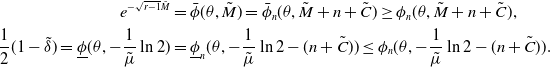 \begin{align*} e^{-\sqrt {r-1}\tilde {M}} & = \bar {\phi }(\theta, \tilde {M})=\bar {\phi }_n(\theta, \tilde {M}+n+\tilde {C})\ge \phi _n(\theta, \tilde {M}+n+\tilde {C}),\\\frac {1}{2}(1-\tilde {\delta })=\underline {\phi }(\theta, -\frac {1}{\tilde {\mu }}\ln 2) & = \underline {\phi }_n(\theta, -\frac {1}{\tilde {\mu }}\ln 2-(n+\tilde {C}))\le \phi _n(\theta, -\frac {1}{\tilde {\mu }}\ln 2-(n+\tilde {C})). \end{align*}
Define $b_n\,:\!=\,\sup \limits _{}\{x\ :\ \phi _n(\theta, x)\in [\frac{1}{2}(1-\tilde{\delta }),1]\}$
. In other word,
$b_n\,:\!=\,\sup \limits _{}\{x\ :\ \phi _n(\theta, x)\in [\frac{1}{2}(1-\tilde{\delta }),1]\}$
. In other word, $b_n$
is a point so that
$b_n$
is a point so that $\phi _n(\theta, b_n)=\frac 12 (1-\tilde{\delta })$
. Then
$\phi _n(\theta, b_n)=\frac 12 (1-\tilde{\delta })$
. Then $-\frac{1}{\tilde{\mu }}\ln 2-(n+\tilde{C})\le b_n\le \tilde{M}+n+\tilde{C}$
. Let
$-\frac{1}{\tilde{\mu }}\ln 2-(n+\tilde{C})\le b_n\le \tilde{M}+n+\tilde{C}$
. Let $\phi _{+,n}(\theta, x)\,:\!=\,\phi _n(\theta, x+b_n)$
. Then we have
$\phi _{+,n}(\theta, x)\,:\!=\,\phi _n(\theta, x+b_n)$
. Then we have
 \begin{align*} \phi _{+,n}=\phi _n(\theta, {\cdot}+b_n)=G_n[\phi _n](\theta, {\cdot}+b_n)=Q[\phi _n(\theta, \kappa _n({\cdot}+b_n))]\in Q[C_{\beta }]. \end{align*}
By the solution of the integral form of system (2.3), we have
 \begin{align*} \phi _{+,n}(\theta, x)=\int _{\mathbb {R}}\bar {G}(x-y,1)\phi _n(\theta, \kappa _n(y+b_n) )dy+\int _{0}^{1}\int _{\mathbb {R}}\bar {G}(x-y,1-s)\bar {f}(\phi (1,y))dyds, \end{align*}
where $\bar{f}(\phi )=\phi (1-r-\phi +r(K*\mathcal{L}_{b,c}\phi ))$
is the reaction term of (2.3) and
$\bar{f}(\phi )=\phi (1-r-\phi +r(K*\mathcal{L}_{b,c}\phi ))$
is the reaction term of (2.3) and $\bar{G}$
is the fundamental solution of
$\bar{G}$
is the fundamental solution of $u_t=u_{xx}$
. By calculation, we have
$u_t=u_{xx}$
. By calculation, we have $|(\phi _{+,n})_{x}(\theta, x)|\lt \frac{1}{\sqrt{2\pi }}+\sqrt{\frac{2}{\pi }}$
. Therefore,
$|(\phi _{+,n})_{x}(\theta, x)|\lt \frac{1}{\sqrt{2\pi }}+\sqrt{\frac{2}{\pi }}$
. Therefore, $\phi _{+,n}$
is equicontinuous and uniformly bounded. According to the Ascoli–Arzela theorem, there exist a subsequence (denoted by
$\phi _{+,n}$
is equicontinuous and uniformly bounded. According to the Ascoli–Arzela theorem, there exist a subsequence (denoted by $n$
), a non-increasing function
$n$
), a non-increasing function $\phi _+$
, and
$\phi _+$
, and $\xi _+$
such that
$\xi _+$
such that
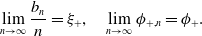 \begin{align*} \lim \limits _{n\rightarrow \infty }\frac {b_n}{n}=\xi _+, \quad \lim \limits _{n\rightarrow \infty } \phi _{+,n}=\phi _+. \end{align*}
Define $C_+\,:\!=\,\tilde{C}\xi _+.$
Observe that
$C_+\,:\!=\,\tilde{C}\xi _+.$
Observe that
 \begin{align*} \lim \limits _{n\rightarrow \infty }\kappa _n(x+b_n)-b_n=\lim \limits _{n\rightarrow \infty }(x+\tilde {C}{\cdot}\frac {x+b_n}{n})=x+C_+ \end{align*}
holds uniformly for $x$
in any bounded subset of
$x$
in any bounded subset of $\mathbb{R}$
. For any
$\mathbb{R}$
. For any $x\in \mathbb{R}$
, we have
$x\in \mathbb{R}$
, we have
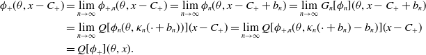 \begin{equation} \begin{aligned} \phi _+(\theta, x-C_+)&=\lim \limits _{n\rightarrow \infty } \phi _{+,n}(\theta, x-C_+)=\lim \limits _{n\rightarrow \infty }\phi _n(\theta, x-C_++b_n)=\lim \limits _{n\rightarrow \infty }G_n[\phi _n](\theta, x-C_++b_n)\\ &=\lim \limits _{n\rightarrow \infty }Q[\phi _n(\theta, \kappa _n({\cdot}+b_n))](x-C_+)=\lim \limits _{n\rightarrow \infty }Q[\phi _{+,n}(\theta, \kappa _n({\cdot}+b_n)-b_n)](x-C_+)\\ &=Q[\phi _+](\theta, x). \end{aligned} \end{equation}
Consequently, $\phi _+(\theta, -\infty )$
and
$\phi _+(\theta, -\infty )$
and $\phi _+(\theta, \infty )$
are fixed points of
$\phi _+(\theta, \infty )$
are fixed points of $Q$
. Observing that
$Q$
. Observing that $\frac{1}{2}(1-\tilde{\delta })\le \lim \limits _{n\rightarrow \infty }\phi _n(\theta, b_n)=\phi _+(\theta, 0)\lt 1$
. It follows that
$\frac{1}{2}(1-\tilde{\delta })\le \lim \limits _{n\rightarrow \infty }\phi _n(\theta, b_n)=\phi _+(\theta, 0)\lt 1$
. It follows that $\phi _+(\theta, -\infty )=1$
and
$\phi _+(\theta, -\infty )=1$
and $\phi _+(\theta, \infty )=0$
. Hence, the proof is complete.
$\phi _+(\theta, \infty )=0$
. Hence, the proof is complete.
The solution to equation (2.3) exhibits continuity with respect to its parameter $c$
, which implies that
$c$
, which implies that $C_+$
is a continuous function of
$C_+$
is a continuous function of $c$
. By substituting
$c$
. By substituting $C_+=C(c)$
back into equation (2.3), we shall present the following theorem.
$C_+=C(c)$
back into equation (2.3), we shall present the following theorem.
Theorem 2.5.
Assume that H1 and (K1) hold. There exist $C(c)\in \mathbb{R}$
and
$C(c)\in \mathbb{R}$
and $\Phi \in \mathcal{M}_\beta$
connecting
$\Phi \in \mathcal{M}_\beta$
connecting $\beta$
to
$\beta$
to $0$
such that
$0$
such that $Q_t[\Phi ](\theta, x)=\Phi (\theta, x-C(c)t)$
for all
$Q_t[\Phi ](\theta, x)=\Phi (\theta, x-C(c)t)$
for all $x\in \mathbb{R}$
,
$x\in \mathbb{R}$
, $\theta \in ({-}\infty, 0]$
, that is, (2.3) admits a non-increasing travelling wave
$\theta \in ({-}\infty, 0]$
, that is, (2.3) admits a non-increasing travelling wave $\Phi (\theta, x-C(c)t)$
connecting
$\Phi (\theta, x-C(c)t)$
connecting $\beta$
to
$\beta$
to $0$
. Furthermore, this bistable travelling wave
$0$
. Furthermore, this bistable travelling wave $\Phi (\theta, z)$
is strictly decreasing in
$\Phi (\theta, z)$
is strictly decreasing in $z$
with
$z$
with $\Phi _z(\theta, z)\lt 0$
. The wave speed
$\Phi _z(\theta, z)\lt 0$
. The wave speed $C(c)$
is non-increasing with respect to
$C(c)$
is non-increasing with respect to $c$
, which means
$c$
, which means $C(c_1)\ge C(c_2)$
if
$C(c_1)\ge C(c_2)$
if $0\lt c_1\le c_2$
.
$0\lt c_1\le c_2$
.
Proof. The existence of $\Phi$
in (2.3) connecting
$\Phi$
in (2.3) connecting $\beta$
to
$\beta$
to $0$
can be guaranteed by Theorem2.4. We now prove
$0$
can be guaranteed by Theorem2.4. We now prove $\Phi _z(\theta, z)\lt 0$
by a contradiction argument. Assume
$\Phi _z(\theta, z)\lt 0$
by a contradiction argument. Assume $\Phi _z(\theta, z_0)=0$
for some
$\Phi _z(\theta, z_0)=0$
for some $z_0\in \mathbb{R}$
. The strong maximum principle implies that
$z_0\in \mathbb{R}$
. The strong maximum principle implies that $\Phi _z(\theta, z)\equiv 0$
for
$\Phi _z(\theta, z)\equiv 0$
for $z\in \mathbb{R}$
. It contradicts the boundary condition (2.5). Next, we will show the monotonicity of
$z\in \mathbb{R}$
. It contradicts the boundary condition (2.5). Next, we will show the monotonicity of $C(c)$
with respect to
$C(c)$
with respect to $c$
. Let
$c$
. Let $0\lt c_1\le c_2$
. By taking the maximum value, we can set a same
$0\lt c_1\le c_2$
. By taking the maximum value, we can set a same $\tilde{C}$
in Lemma 2.2 for both
$\tilde{C}$
in Lemma 2.2 for both $c=c_1$
and
$c=c_1$
and $c=c_2$
. According to Lemma 2.1
$c=c_2$
. According to Lemma 2.1 $c)$
, we conclude that the reaction term in (2.4) is non-increasing with respect to
$c)$
, we conclude that the reaction term in (2.4) is non-increasing with respect to $c$
. From Lemma 2.3, we have
$c$
. From Lemma 2.3, we have $\phi _n(c_1,\theta, \tilde{x})\ge \phi _n(c_2, \theta, \tilde{x})$
(here
$\phi _n(c_1,\theta, \tilde{x})\ge \phi _n(c_2, \theta, \tilde{x})$
(here $\phi _n(c, \theta, \tilde{x})$
implies that
$\phi _n(c, \theta, \tilde{x})$
implies that $\phi _n$
is dependent on
$\phi _n$
is dependent on $c$
). Based on the proof of Theorem2.4, we know that
$c$
). Based on the proof of Theorem2.4, we know that $b_n(c_1)\ge b_n(c_2)$
(Here
$b_n(c_1)\ge b_n(c_2)$
(Here $b_n(c)$
indicates that
$b_n(c)$
indicates that $b_n$
is dependent on
$b_n$
is dependent on $c$
). Consequently,
$c$
). Consequently, $C(c_1)\ge C(c_2)$
. Therefore, the proof is complete.
$C(c_1)\ge C(c_2)$
. Therefore, the proof is complete.
2.2. Bistable waves of the original system (1.5)-(1.6)
To establish the existence and uniqueness of a bistable monotone travelling wave for (1.5)-(1.6) under H1, we first crucially show that the equation $C(c) = c$
possesses a unique positive root. This leads us to the following theorem.
$C(c) = c$
possesses a unique positive root. This leads us to the following theorem.
Theorem 2.6.
Assume that H1 and (K1) hold. There exists a monotone bistable travelling wave $(c, \Phi (z), \Psi (z))$
,
$(c, \Phi (z), \Psi (z))$
, $z=\nu {\cdot}x-ct$
,
$z=\nu {\cdot}x-ct$
, $||\nu ||=1$
, of system (1.5)-(1.6), where
$||\nu ||=1$
, of system (1.5)-(1.6), where $c$
is positive and unique. Moreover,
$c$
is positive and unique. Moreover, $\Phi ^{\prime}(z)\lt 0$
and
$\Phi ^{\prime}(z)\lt 0$
and $\Psi ^{\prime}(z)\lt 0$
for
$\Psi ^{\prime}(z)\lt 0$
for $z\in \mathbb{R}$
.
$z\in \mathbb{R}$
.
Proof. Theorem2.5 gives the existence of the monotone bistable travelling wave solution of (2.4)-(2.5). We also know that $C(c)$
is a non-increasing function of
$C(c)$
is a non-increasing function of $c$
. To return to (1.5)-(1.6) for the existence of waves, we need to show that
$c$
. To return to (1.5)-(1.6) for the existence of waves, we need to show that $C(c)=c$
has a unique positive root. To this end, it suffices to show
$C(c)=c$
has a unique positive root. To this end, it suffices to show $C(0_+)\gt 0$
. Let
$C(0_+)\gt 0$
. Let
 \begin{align*} f(\Phi )=\Phi (1-r-\Phi +r(K\star _C\mathcal {L}_{b,c}\Phi )). \end{align*}
Then (2.4) can be written as
 \begin{equation} \Phi ^{\prime\prime}+C(c,f)\Phi ^{\prime}+f(\Phi )=0. \end{equation}
Here we just use $C(c,f)$
to indicate that the speed is dependent on the reaction term.
$C(c,f)$
to indicate that the speed is dependent on the reaction term.
By Lemma 2.1 $c)$
, there exist a sufficiently small
$c)$
, there exist a sufficiently small $\delta \gt 0$
such that
$\delta \gt 0$
such that $\mathcal{L}_{b,c}\Phi (z)\gt 1-\delta$
for sufficiently small
$\mathcal{L}_{b,c}\Phi (z)\gt 1-\delta$
for sufficiently small $c\lt \delta$
and
$c\lt \delta$
and $\Phi \gt 0$
. Then, for small
$\Phi \gt 0$
. Then, for small $\hat{\varepsilon }\gt 0$
, we have
$\hat{\varepsilon }\gt 0$
, we have
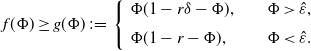 \begin{equation} f(\Phi )\ge g(\Phi )\,:\!=\,\left \{ \begin{array}{cc} \begin{aligned} &\Phi (1-r\delta -\Phi ),\quad & \Phi \gt \hat{\varepsilon }, \\[3pt] &\Phi (1-r-\Phi ),\ &\Phi \lt \hat{\varepsilon }.\\ \end{aligned} \end{array} \right . \end{equation}
Consider
 \begin{equation} \Phi ^{\prime\prime}+C(c,g)\Phi ^{\prime}+g(\Phi )=0. \end{equation}
By choosing $\tilde{\delta }$
in (2.6) such that
$\tilde{\delta }$
in (2.6) such that $\tilde{\delta }-r\delta \gt 0$
, we can derive the existence of
$\tilde{\delta }-r\delta \gt 0$
, we can derive the existence of $\Phi (z)$
in (2.19) connecting
$\Phi (z)$
in (2.19) connecting $1-r\delta$
to
$1-r\delta$
to $0$
according to the similar arguments in Lemmas 2.2 and 2.3, and Theorem2.4. We multiply the left and right sides of (2.19) by
$0$
according to the similar arguments in Lemmas 2.2 and 2.3, and Theorem2.4. We multiply the left and right sides of (2.19) by $\Phi ^{\prime}$
and integrate both sides from
$\Phi ^{\prime}$
and integrate both sides from $-\infty$
to
$-\infty$
to $\infty$
with respect to
$\infty$
with respect to $z$
. It follows that the wave speed
$z$
. It follows that the wave speed $C(c,g)$
satisfies
$C(c,g)$
satisfies
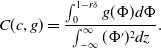 \begin{align*} C(c,g)=\frac {\int _{0}^{1-r\delta }g(\Phi )d\Phi }{\int _{-\infty }^{\infty }(\Phi ^{\prime})^2dz}. \end{align*}
Since $\hat{\varepsilon }$
and
$\hat{\varepsilon }$
and $\delta$
are small enough, we have
$\delta$
are small enough, we have
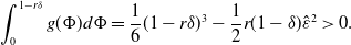 \begin{align*}\int _{0}^{1-r\delta }g(\Phi )d\Phi =\frac {1}{6}(1-r \delta )^3-\frac {1}{2}r(1-\delta )\hat {\varepsilon }^2\gt 0.\end{align*}
It means $C(c,g)\gt 0$
. Applying equations (2.17), (2.18), (2.19), and a similar proof as presented in Theorem2.5(concerning the monotonicity of
$C(c,g)\gt 0$
. Applying equations (2.17), (2.18), (2.19), and a similar proof as presented in Theorem2.5(concerning the monotonicity of $C(c)$
with respect to
$C(c)$
with respect to $c$
), we can deduce that
$c$
), we can deduce that $C(c,f)\ge C(c,g)\gt 0$
when
$C(c,f)\ge C(c,g)\gt 0$
when $c \rightarrow 0$
. According to Theorem2.5, the equation
$c \rightarrow 0$
. According to Theorem2.5, the equation $C(c)=c$
has a unique positive solution. Consequently, system (2.2) has a monotonic solution
$C(c)=c$
has a unique positive solution. Consequently, system (2.2) has a monotonic solution $(c,\Phi (z))$
, that is, there exists a monotone bistable travelling wave
$(c,\Phi (z))$
, that is, there exists a monotone bistable travelling wave $(c, \Phi (z), \Psi (z))$
of system (1.5)-(1.6). Based on Lemma 2.1 and Theorem2.5, we know
$(c, \Phi (z), \Psi (z))$
of system (1.5)-(1.6). Based on Lemma 2.1 and Theorem2.5, we know $\Phi ^{\prime}(z)\lt 0$
and
$\Phi ^{\prime}(z)\lt 0$
and $\Psi ^{\prime}(z)\lt 0$
for
$\Psi ^{\prime}(z)\lt 0$
for $z\in \mathbb{R}$
. It completes the proof.
$z\in \mathbb{R}$
. It completes the proof.
Our aim in the subsequent discussion is to establish the uniqueness of the above travelling wave profiles. To achieve this, we utilise the bistable travelling wave $(\Phi (z),\Psi (z))$
to create a pair of upper and lower solutions of (1.2). We introduce two non-increasing continuous functions
$(\Phi (z),\Psi (z))$
to create a pair of upper and lower solutions of (1.2). We introduce two non-increasing continuous functions
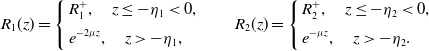 \begin{equation} R_1(z)=\left \{ \begin{aligned}& R_1^+, \quad z\le -\eta _1\lt 0,\\[3pt] &e^{-2\mu z}, \quad z\gt -\eta _1,\\ \end{aligned}\right . \quad \quad R_2(z)=\left \{ \begin{aligned}& R_2^+, \quad z\le -\eta _2\lt 0,\\[3pt] &e^{-\mu z}, \quad z\gt -\eta _2.\\ \end{aligned}\right . \end{equation}
Here constants $R_i^{+}\gt 1$
, i = 1,2, and
$R_i^{+}\gt 1$
, i = 1,2, and $\mu \gt 0$
is small to be determined.
$\mu \gt 0$
is small to be determined. $\eta _1$
and
$\eta _1$
and $\eta _2$
are chosen so that the above two functions are continuous. We first give the following squeezing lemma, which is crucial in proving the uniqueness of the bistable travelling wave of (1.5)-(1.6).
$\eta _2$
are chosen so that the above two functions are continuous. We first give the following squeezing lemma, which is crucial in proving the uniqueness of the bistable travelling wave of (1.5)-(1.6).
Lemma 2.7. Assume that H1, (K1) and (K2) hold. Define
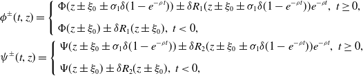 \begin{align*} \begin {aligned} &\phi ^{\pm }(t,z)=\left \{ \begin {aligned} &\Phi (z\pm \xi _0\pm \sigma _1\delta (1-e^{-\rho t}))\pm \delta R_1(z\pm \xi _0\pm \sigma _1\delta (1-e^{-\rho t}))e^{-\rho t},\ t\ge 0,\\[5pt] &\Phi (z\pm \xi _0)\pm \delta R_1(z\pm \xi _0),\ t\lt 0,\\ \end {aligned}\right .\\ & \psi ^{\pm }(t,z)=\left \{ \begin {aligned} & \Psi (z\pm \xi _0\pm \sigma _1\delta (1-e^{-\rho t}))\pm \delta R_2(z\pm \xi _0\pm \sigma _1\delta (1-e^{-\rho t}))e^{-\rho t}, \ t\ge 0, \\[5pt] & \Psi (z\pm \xi _0)\pm \delta R_2(z\pm \xi _0), \ t\lt 0,\\ \end {aligned}\right . \end {aligned} \end{align*}
where $z=\nu {\cdot}x-ct$
and
$z=\nu {\cdot}x-ct$
and $ ||\nu ||=1$
. Then there exists
$ ||\nu ||=1$
. Then there exists $\sigma _1\lt 0$
,
$\sigma _1\lt 0$
, $\mu \gt 0$
,
$\mu \gt 0$
, $\rho \gt 0$
and
$\rho \gt 0$
and $\delta _0\gt 0$
such that for any
$\delta _0\gt 0$
such that for any $\xi _0\in \mathbb{R}$
,
$\xi _0\in \mathbb{R}$
, $\delta \in (0,\delta _0)$
, the formulas
$\delta \in (0,\delta _0)$
, the formulas $(\phi ^{\pm }(t,z),\psi ^{\pm }(t,z))$
are upper and lower solutions of (1.2), respectively. It further follows that
$(\phi ^{\pm }(t,z),\psi ^{\pm }(t,z))$
are upper and lower solutions of (1.2), respectively. It further follows that $(\phi ^{-}(t,z), \psi ^{-}(t,z))\le (\phi (t,z), \psi (t,z))\le (\phi ^{+}(t,z),\psi ^{+}(t,z))$
for
$(\phi ^{-}(t,z), \psi ^{-}(t,z))\le (\phi (t,z), \psi (t,z))\le (\phi ^{+}(t,z),\psi ^{+}(t,z))$
for $(t, z)\in (0, \infty ]\times \mathbb{R}$
, if
$(t, z)\in (0, \infty ]\times \mathbb{R}$
, if $(\phi ^{-}(\theta, z), \psi ^{-}(\theta, z))\le (\phi (\theta, z), \psi (\theta, z))\le (\phi ^{+}(\theta, z),\psi ^{+}(\theta, z))$
for
$(\phi ^{-}(\theta, z), \psi ^{-}(\theta, z))\le (\phi (\theta, z), \psi (\theta, z))\le (\phi ^{+}(\theta, z),\psi ^{+}(\theta, z))$
for $(\theta, z)\in ({-}\infty, 0]\times \mathbb{R}$
.
$(\theta, z)\in ({-}\infty, 0]\times \mathbb{R}$
.
Proof. We only prove $(\phi ^+(t,z), \psi ^+(t,z))$
is an upper solution of (1.2), while the lower solution
$(\phi ^+(t,z), \psi ^+(t,z))$
is an upper solution of (1.2), while the lower solution $(\phi ^-(t,z), \psi ^-(t,z))$
can be verified using a similar argument. Let
$(\phi ^-(t,z), \psi ^-(t,z))$
can be verified using a similar argument. Let $\xi =z+ \xi _0+ \sigma _1\delta (1-e^{-\rho t})$
. We choose
$\xi =z+ \xi _0+ \sigma _1\delta (1-e^{-\rho t})$
. We choose $\delta$
,
$\delta$
, $\mu$
and
$\mu$
and $\rho \lt \min \{\mu ^2,\tilde{\delta }_0\}$
that are small enough, where
$\rho \lt \min \{\mu ^2,\tilde{\delta }_0\}$
that are small enough, where $\tilde{\delta }_0$
is defined in (K2). We take
$\tilde{\delta }_0$
is defined in (K2). We take $R_1^+$
and
$R_1^+$
and $R_2^+$
such that
$R_2^+$
such that
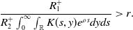 \begin{align*}\frac {R_1^+}{R_2^+\int _{0}^{\infty }\int _{\mathbb {R}}K(s,y)e^{\rho s}dyds}\gt r.\end{align*}
For small enough $\epsilon _1\gt 0$
,
$\epsilon _1\gt 0$
, $\epsilon _3\gt 0$
and
$\epsilon _3\gt 0$
and $\epsilon _4\gt 0$
, we take sufficiently large
$\epsilon _4\gt 0$
, we take sufficiently large $M_1\gt \frac{1}{\mu ^2}$
such that
$M_1\gt \frac{1}{\mu ^2}$
such that $\Phi (z), \Psi (z)\lt \epsilon _1$
for
$\Phi (z), \Psi (z)\lt \epsilon _1$
for $\xi \gt \frac{M_1}{2}$
and
$\xi \gt \frac{M_1}{2}$
and
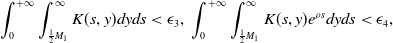 \begin{align*}\int _{0}^{+\infty }\int _{\frac {1}{2}M_1}^\infty K(s,y)dyds\lt \epsilon _3,\ \int _{0}^{+\infty }\int _{\frac {1}{2}M_1}^\infty K(s,y)e^{\rho s}dyds\lt \epsilon _4,\end{align*}
by using (K1) and (K2). Take $M_2\gt 0$
and sufficiently small
$M_2\gt 0$
and sufficiently small $\epsilon _2\gt 0$
such that
$\epsilon _2\gt 0$
such that $\Phi (z), \Psi (z)\gt 1-\epsilon _2$
for
$\Phi (z), \Psi (z)\gt 1-\epsilon _2$
for $\xi \lt -M_2$
.
$\xi \lt -M_2$
.
Let $M\gt \max \{\eta _1, \eta _2, M_1, M_2\}$
. Set
$M\gt \max \{\eta _1, \eta _2, M_1, M_2\}$
. Set
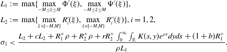 \begin{equation} \begin{aligned} &L_1\,:\!=\,\max \{\max _{-M\le \xi \le M}\Phi ^{\prime}(\xi ), \max _{-M\le \xi \le M}\Psi ^{\prime}(\xi )\},\\ &L_2\,:\!=\,\max \{ \max _{\xi \in [{-}M, M]}R_i^{\prime}(\xi ), \max _{\xi \in [{-}M, M]}R_i^{\prime\prime}(\xi ) \}, i=1,2,\\ &\sigma _1\lt \frac{L_2+cL_2+R_1^+\rho +R_2^+\rho + rR_2^+\int _{0}^{\infty }\int _{\mathbb{R}}K(s,y)e^{\rho s}dyds+(1+b)R_1^+}{\rho L_1}. \end{aligned} \end{equation}
Substituting $(\phi ^+,\psi ^+)$
into (1.2), we get
$(\phi ^+,\psi ^+)$
into (1.2), we get
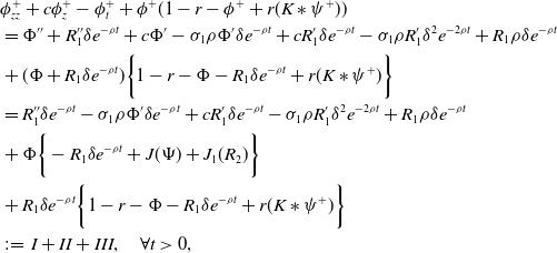 \begin{equation} \begin{aligned} &\phi ^+_{zz}+c\phi ^+_{z}-\phi ^+_{t}+\phi ^+(1-r-\phi ^++r(K*\psi ^+))\\ & =\Phi ^{\prime\prime}+R_1^{\prime\prime}\delta e^{-\rho t} +c\Phi ^{\prime}-\sigma _1 \rho \Phi ^{\prime}\delta e^{-\rho t} +cR_1^{\prime}\delta e^{-\rho t} -\sigma _1\rho R_1^{\prime}\delta ^2 e^{-2\rho t} +R_1\rho \delta e^{-\rho t}\\ &+(\Phi +R_1\delta e^{-\rho t})\bigg \{ 1-r-\Phi -R_1\delta e^{-\rho t}+r(K*\psi ^+)\bigg \}\\ &=R_1^{\prime\prime}\delta e^{-\rho t}-\sigma _1 \rho \Phi ^{\prime}\delta e^{-\rho t} +cR_1^{\prime}\delta e^{-\rho t} -\sigma _1\rho R_1^{\prime}\delta ^2 e^{-2\rho t} +R_1\rho \delta e^{-\rho t}\\ &+\Phi \bigg \{-R_1\delta e^{-\rho t}+J(\Psi )+J_1(R_2)\bigg \}\\ &+R_1\delta e^{-\rho t}\bigg \{ 1-r-\Phi -R_1\delta e^{-\rho t}+r(K*\psi ^+)\bigg \}\\ &\,:\!=\,I+II+III, \quad \forall t\gt 0, \end{aligned} \end{equation}
where
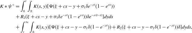 \begin{align*} \begin {aligned} K*\psi ^+ & =\int _{0}^{t}\int _{\mathbb {R}}K(s,y)[\Psi (\xi +cs-y+\sigma _1\delta e^{-\rho t}(1-e^{\rho s})) \nonumber\\ & +R_2(\xi +cs-y+\sigma _1\delta e^{-\rho t}(1-e^{\rho s}))\delta e^{-\rho (t-s)}]dyds\\ &+\int _{t}^{\infty }\int _{\mathbb {R}}K(s,y)[\Psi (\xi +cs-y-\sigma _1\delta (1-e^{-\rho t}))+R_2(\xi +cs-y-\sigma _1\delta (1-e^{-\rho t}))\delta ]dyds, \end {aligned} \end{align*}
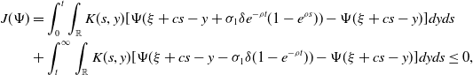 \begin{align*} \begin {aligned} J(\Psi )&=\int _{0}^{t}\int _{\mathbb {R}}K(s,y)[\Psi (\xi +cs-y+\sigma _1\delta e^{-\rho t}(1-e^{\rho s}))-\Psi (\xi +cs-y)]dyds\\ &+\int _{t}^{\infty }\int _{\mathbb {R}}K(s,y)[\Psi (\xi +cs-y-\sigma _1\delta (1-e^{-\rho t}))-\Psi (\xi +cs-y)]dyds\le 0, \end {aligned} \end{align*}
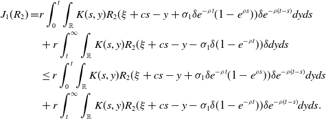 \begin{align*} \begin {aligned} J_1(R_2)=& r\int _{0}^{t}\int _{\mathbb {R}}K(s,y)R_2(\xi +cs-y+\sigma _1\delta e^{-\rho t}(1-e^{\rho s}))\delta e^{-\rho (t-s)}dyds\\ &+ r\int _{t}^{\infty }\int _{\mathbb {R}}K(s,y)R_2(\xi +cs-y-\sigma _1\delta (1-e^{-\rho t}))\delta dyds\\ &\le r\int _{0}^{t}\int _{\mathbb {R}}K(s,y)R_2(\xi +cs-y+\sigma _1\delta e^{-\rho t}(1-e^{\rho s}))\delta e^{-\rho (t-s)}dyds\\ &+ r\int _{t}^{\infty }\int _{\mathbb {R}}K(s,y)R_2(\xi +cs-y-\sigma _1\delta (1-e^{-\rho t}))\delta e^{-\rho (t-s)}dyds.\\ \end {aligned} \end{align*}
and
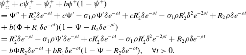 \begin{equation} \begin{aligned} &\psi ^+_{zz}+c\psi ^+_{z}-\psi ^+_{t}+b\phi ^+(1-\psi ^+)\\ &=\Psi ^{\prime\prime}+R_2^{\prime\prime}\delta e^{-\rho t}+c\Psi ^{\prime}-\sigma _1\rho \Psi ^{\prime}\delta e^{-\rho t}+cR_2^{\prime}\delta e^{-\rho t}-\sigma _1\rho R_2^{\prime}\delta ^2 e^{-2\rho t}+R_2\rho \delta e^{-\rho t} \\ &+b(\Phi +R_1\delta e^{-\rho t})(1-\Psi -R_2\delta e^{-\rho t})\\ &=R_2^{\prime\prime}\delta e^{-\rho t}-\sigma _1\rho \Psi ^{\prime}\delta e^{-\rho t}+cR_2^{\prime}\delta e^{-\rho t}-\sigma _1\rho R_2^{\prime}\delta ^2 e^{-2\rho t}+R_2\rho \delta e^{-\rho t} \\ &-b\Phi R_2\delta e^{-\rho t}+bR_1\delta e^{-\rho t}(1-\Psi -R_2\delta e^{-\rho t}), \quad \forall t\gt 0. \end{aligned} \end{equation}
Here we use the fact $(\Phi, \Psi )$
is the bistable travelling wave of (1.2) and satisfies (1.5). In order to prove
$(\Phi, \Psi )$
is the bistable travelling wave of (1.2) and satisfies (1.5). In order to prove $(\phi ^+(z,t),\psi ^+(z,t))$
is an upper solution of (1.2), we consider three cases:
$(\phi ^+(z,t),\psi ^+(z,t))$
is an upper solution of (1.2), we consider three cases:
Case (i): $|\xi |\le M$
. According to (2.21) and (2.22), we have
$|\xi |\le M$
. According to (2.21) and (2.22), we have
 \begin{align*} I\le \delta e^{-\rho t}[L_2-\sigma _1\rho L_1+cL_2+R_1^+\rho ], \end{align*}
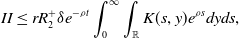 \begin{align*} II\le rR_2^+ \delta e^{-\rho t}\int _{0}^{\infty }\int _{\mathbb {R}}K(s,y)e^{\rho s}dyds, \end{align*}
and
 \begin{align*} III\le R_1^+\delta e^{-\rho t}[1-r+r(1+R_2^+\delta e^{-\rho t}\int _{0}^{\infty }\int _{\mathbb {R}}K(s,y)e^{\rho s}dyds)]. \end{align*}
Then it gives
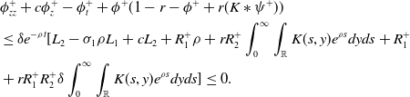 \begin{equation} \begin{aligned} &\phi ^+_{zz}+c\phi ^+_{z}-\phi ^+_{t}+\phi ^+(1-r-\phi ^++r(K*\psi ^+))\\ &\le \delta e^{-\rho t}[L_2-\sigma _1\rho L_1+cL_2+R_1^+\rho +rR_2^+\int _{0}^{\infty }\int _{\mathbb{R}}K(s,y)e^{\rho s}dyds+R_1^+\\ &+rR_1^+R_2^+\delta \int _{0}^{\infty }\int _{\mathbb{R}}K(s,y)e^{\rho s}dyds]\le 0. \end{aligned} \end{equation}
The last inequality sign in (2.24) holds by (K2), (2.21) and $\delta$
is sufficiently small. By (2.21) and (2.23), we also have
$\delta$
is sufficiently small. By (2.21) and (2.23), we also have
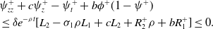 \begin{equation} \begin{aligned} &\psi ^+_{zz}+c\psi ^+_{z}-\psi ^+_{t}+b\phi ^+(1-\psi ^+)\\ &\le \delta e^{-\rho t}[L_2-\sigma _1\rho L_1+cL_2+R_2^+\rho +bR_1^+]\le 0. \end{aligned} \end{equation}
Case (ii): $\xi \lt -M$
. Note that
$\xi \lt -M$
. Note that $\xi \lt -M_2$
,
$\xi \lt -M_2$
, $R_1(\xi )=R_1^+$
and
$R_1(\xi )=R_1^+$
and $R_2(\xi )=R_2^+$
. According to (2.22) and the fact
$R_2(\xi )=R_2^+$
. According to (2.22) and the fact $\frac{R_1^+}{R_2^+\int _{0}^{\infty }\int _{\mathbb{R}}K(s,y)e^{\rho s}dyds}\gt r$
, we have
$\frac{R_1^+}{R_2^+\int _{0}^{\infty }\int _{\mathbb{R}}K(s,y)e^{\rho s}dyds}\gt r$
, we have
 \begin{align*} I\le R_1^+\rho \delta e^{-\rho t}, \end{align*}
 \begin{align*} II\le \Phi \delta e^{-\rho t}({-}R_1^++rR_2^+\int _{0}^{\infty }\int _{\mathbb {R}}K(s,y)e^{\rho s}dyds)\le \delta e^{-\rho t}(1-\epsilon _2)({-}R_1^++rR_2^+\int _{0}^{\infty }\int _{\mathbb {R}}K(s,y)e^{\rho s}dyds), \end{align*}
and
 \begin{align*} III\le R_1^+\delta e^{-\rho t}[1-r-(1-\epsilon _2)+r(1+R_2^+\delta e^{-\rho t}\int _{0}^{\infty }\int _{\mathbb {R}}K(s,y)e^{\rho s}dyds)]. \end{align*}
Then
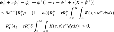 \begin{equation} \begin{aligned} &\phi ^+_{zz}+c\phi ^+_{z}-\phi ^+_{t}+\phi ^+(1-r-\phi ^++r(K*\psi ^+))\\ &\le \delta e^{-\rho t}[R_1^+\rho -(1-\epsilon _2)(R_1^+-rR_2^+\int _{0}^{\infty }\int _{\mathbb{R}}K(s,y)e^{\rho s}dyds)\\ &+R_1^+(\epsilon _2+rR_2^+\delta \int _{0}^{\infty }\int _{\mathbb{R}}K(s,y)e^{\rho s}dyds)]\le 0, \end{aligned} \end{equation}
since $\frac{R_1^+}{R_2^+\int _{0}^{\infty }\int _{\mathbb{R}}K(s,y)e^{\rho s}dyds}\gt r$
, and
$\frac{R_1^+}{R_2^+\int _{0}^{\infty }\int _{\mathbb{R}}K(s,y)e^{\rho s}dyds}\gt r$
, and $\rho$
,
$\rho$
, $\epsilon _2$
,
$\epsilon _2$
, $\delta$
are small enough. By (2.23), we have
$\delta$
are small enough. By (2.23), we have
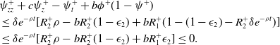 \begin{equation} \begin{aligned} &\psi ^+_{zz}+c\psi ^+_{z}-\psi ^+_{t}+b\phi ^+(1-\psi ^+)\\ &\le \delta e^{-\rho t}[R_2^+\rho -bR_2^+(1-\epsilon _2)+bR_1^+(1-(1-\epsilon _2)-R_2^+\delta e^{-\rho t})]\\ &\le \delta e^{-\rho t}[R_2^+\rho -bR_2^+(1-\epsilon _2)+bR_1^+\epsilon _2]\le 0. \end{aligned} \end{equation}
The last inequality in (2.27) holds since $\rho$
and
$\rho$
and $\epsilon _2$
are small enough.
$\epsilon _2$
are small enough.
Case (iii): $\xi \gt M$
. Note that
$\xi \gt M$
. Note that $\xi \gt M_1$
,
$\xi \gt M_1$
, $R_1(\xi )=e^{-2\mu \xi }$
and
$R_1(\xi )=e^{-2\mu \xi }$
and $R_2(\xi )=e^{-\mu \xi }$
. We can calculate
$R_2(\xi )=e^{-\mu \xi }$
. We can calculate
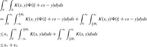 \begin{equation} \begin{aligned} &\int _{0}^{\infty }\int _{\mathbb{R}}K(s,y)\Psi (\xi +cs-y)dyds\\ &=\int _{0}^{\infty }\int _{-\infty }^{\frac{1}{2}M_1}K(s,y)\Psi (\xi +cs-y)dyds+\int _{0}^{\infty }\int _{\frac{1}{2}M_1}^{\infty }K(s,y)\Psi (\xi +cs-y)dyds\\ &\le \epsilon _1\int _{0}^{\infty }\int _{-\infty }^{\frac{1}{2}M_1}K(s,y)dyds+\int _{0}^{\infty }\int _{\frac{1}{2}M_1}^{\infty }K(s,y)dyds\\ &\le \epsilon _1+\epsilon _3 \end{aligned} \end{equation}
and
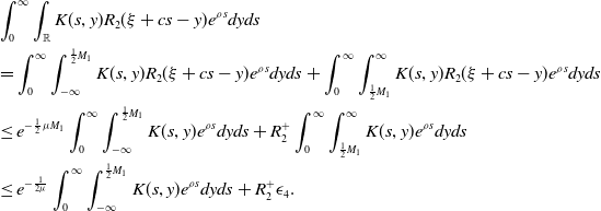 \begin{equation} \begin{aligned} &\int _{0}^{\infty }\int _{\mathbb{R}}K(s,y)R_2(\xi +cs-y)e^{\rho s}dyds\\ &=\int _{0}^{\infty }\int _{-\infty }^{\frac{1}{2}M_1}K(s,y)R_2(\xi +cs-y)e^{\rho s}dyds+\int _{0}^{\infty }\int _{\frac{1}{2}M_1}^{\infty }K(s,y)R_2(\xi +cs-y)e^{\rho s}dyds\\ &\le e^{-\frac{1}{2}\mu M_1}\int _{0}^{\infty }\int _{-\infty }^{\frac{1}{2}M_1}K(s,y)e^{\rho s}dyds+R_2^+\int _{0}^{\infty }\int _{\frac{1}{2}M_1}^{\infty }K(s,y)e^{\rho s}dyds\\ &\le e^{-\frac{1}{2\mu }}\int _{0}^{\infty }\int _{-\infty }^{\frac{1}{2}M_1}K(s,y)e^{\rho s}dyds+R_2^+\epsilon _4. \end{aligned} \end{equation}
According to (2.22), we have
 \begin{align*} I\le e^{-2\mu \xi }\delta e^{-\rho t}(4\mu ^2-2c\mu +\rho ), \end{align*}
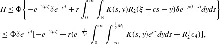 \begin{equation} \begin{aligned} & II\le \Phi \bigg \{{-}e^{-2\mu \xi }\delta e^{-\rho t}+r\int _{0}^{\infty }\int _{\mathbb{R}}K(s,y)R_2(\xi +cs-y)\delta e^{-\rho (t-s)}dyds\bigg \}\\ &\le \Phi \delta e^{-\rho t}[{-}e^{-2\mu \xi }+ r(e^{-\frac{1}{2\mu }}\int _{0}^{\infty }\int _{-\infty }^{\frac{1}{2}M_1}K(s,y)e^{\rho s}dyds+R_2^+\epsilon _4) ], \end{aligned} \end{equation}
and
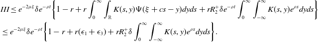 \begin{equation} \begin{aligned} &III\le e^{-2\mu \xi } \delta e^{-\rho t}\bigg \{ 1-r+r\int _{0}^{\infty }\int _{\mathbb{R}}K(s,y)\Psi (\xi +cs-y)dyds+rR_2^+\delta e^{-\rho t} \int _{0}^{\infty }\int _{-\infty }^{\infty }K(s,y)e^{\rho s}dyds \bigg \}\\ &\le e^{-2\mu \xi } \delta e^{-\rho t}\bigg \{ 1-r+r (\epsilon _1+\epsilon _3)+rR_2^+\delta \int _{0}^{\infty }\int _{-\infty }^{\infty }K(s,y)e^{\rho s}dyds \bigg \}. \end{aligned} \end{equation}
Then equation (2.22) becomes
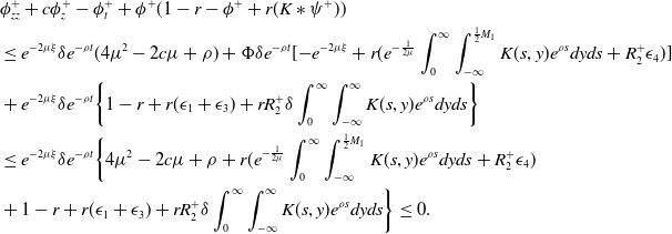 \begin{equation} \begin{aligned} &\phi ^+_{zz}+c\phi ^+_{z}-\phi ^+_{t}+\phi ^+(1-r-\phi ^++r(K*\psi ^+))\\ &\le e^{-2\mu \xi }\delta e^{-\rho t}(4\mu ^2-2c\mu +\rho )+ \Phi \delta e^{-\rho t}[{-}e^{-2\mu \xi }+ r(e^{-\frac{1}{2\mu }}\int _{0}^{\infty }\int _{-\infty }^{\frac{1}{2}M_1}K(s,y)e^{\rho s}dyds+R_2^+\epsilon _4) ]\\ &+e^{-2\mu \xi } \delta e^{-\rho t}\bigg \{ 1-r+r (\epsilon _1+\epsilon _3)+rR_2^+\delta \int _{0}^{\infty }\int _{-\infty }^{\infty }K(s,y)e^{\rho s}dyds \bigg \}\\ &\le e^{-2\mu \xi }\delta e^{-\rho t}\bigg \{ 4\mu ^2-2c\mu +\rho + r(e^{-\frac{1}{2\mu }}\int _{0}^{\infty }\int _{-\infty }^{\frac{1}{2}M_1}K(s,y)e^{\rho s}dyds+R_2^+\epsilon _4)\\ &+1-r+r (\epsilon _1+\epsilon _3)+rR_2^+\delta \int _{0}^{\infty }\int _{-\infty }^{\infty }K(s,y)e^{\rho s}dyds \bigg \}\le 0. \end{aligned} \end{equation}
The last inequality sign in (2.32) holds by (K2), $r\gt 1$
and
$r\gt 1$
and $\mu$
,
$\mu$
, $\rho$
,
$\rho$
, $\epsilon _1$
,
$\epsilon _1$
, $\epsilon _3$
,
$\epsilon _3$
, $\epsilon _4$
,
$\epsilon _4$
, $\delta$
are small enough. It follows from (2.23) that
$\delta$
are small enough. It follows from (2.23) that
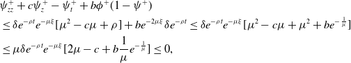 \begin{equation} \begin{aligned} &\psi ^+_{zz}+c\psi ^+_{z}-\psi ^+_{t}+b\phi ^+(1-\psi ^+)\\ &\le \delta e^{-\rho t}e^{-\mu \xi }[\mu ^2-c\mu +\rho ]+be^{-2\mu \xi }\delta e^{-\rho t} \le \delta e^{-\rho t}e^{-\mu \xi }[\mu ^2-c\mu +\mu ^2+be^{-\frac{1}{\mu }}]\\ &\le \mu \delta e^{-\rho t}e^{-\mu \xi }[2\mu -c+b\frac{1}{\mu }e^{-\frac{1}{\mu }}]\le 0, \end{aligned} \end{equation}
since $\rho \lt \mu ^2$
,
$\rho \lt \mu ^2$
, $\xi \gt M_1\gt \frac{1}{\mu ^2}$
, and
$\xi \gt M_1\gt \frac{1}{\mu ^2}$
, and $\mu$
,
$\mu$
, $\frac{1}{\mu }e^{-\frac{1}{\mu }}$
are sufficiently small.
$\frac{1}{\mu }e^{-\frac{1}{\mu }}$
are sufficiently small.
Combining cases (i)-(iii), we know $(\phi ^+(z, t), \psi ^+(z,t))$
is an upper solution of (1.2).
$(\phi ^+(z, t), \psi ^+(z,t))$
is an upper solution of (1.2).
Subsequently, we shall establish the uniqueness of the bistable travelling wave of system (1.2) by using Lemma 2.7.
Theorem 2.8.
Assume that H1, (K1) and (K2) hold. If $(\Phi ^*(\nu\ {\cdot}\ x-c^*t),\Psi ^*(\nu\ {\cdot}\ x-c^*t))$
is a bistable travelling wave of system (1.2) connecting
$(\Phi ^*(\nu\ {\cdot}\ x-c^*t),\Psi ^*(\nu\ {\cdot}\ x-c^*t))$
is a bistable travelling wave of system (1.2) connecting $e_\beta$
to
$e_\beta$
to $e_0$
, then there exists
$e_0$
, then there exists $z^*\in \mathbb{R}$
such that
$z^*\in \mathbb{R}$
such that $(\Phi ^*(\nu\ {\cdot}\ x-c^*t),\Psi ^*(\nu\ {\cdot}\ x-c^*t))=(\Phi (\nu\ {\cdot}\ x-ct+z^*),\Psi (\nu\ {\cdot}\ x-ct+z^*))$
and
$(\Phi ^*(\nu\ {\cdot}\ x-c^*t),\Psi ^*(\nu\ {\cdot}\ x-c^*t))=(\Phi (\nu\ {\cdot}\ x-ct+z^*),\Psi (\nu\ {\cdot}\ x-ct+z^*))$
and $c^*=c$
, where
$c^*=c$
, where $(\Phi (\nu\ {\cdot}\ x-ct),\Psi (\nu\ {\cdot}\ x-ct))$
is the solution in Theorem 2.6.
$(\Phi (\nu\ {\cdot}\ x-ct),\Psi (\nu\ {\cdot}\ x-ct))$
is the solution in Theorem 2.6.
Proof. By using a similar argument in [Reference Trofimchuk, Pinto and Trofimchuk31, Lemma 13], we can conclude the bistable travelling wave of system (1.2) connecting $e_\beta$
to
$e_\beta$
to $e_0$
decays exponentially as
$e_0$
decays exponentially as $z\rightarrow \infty$
. Therefore, there exist
$z\rightarrow \infty$
. Therefore, there exist $\xi _1\in \mathbb{R}$
and
$\xi _1\in \mathbb{R}$
and $h\gg 1$
such that, for
$h\gg 1$
such that, for $\theta \in ({-}\infty, 0]$
, we have
$\theta \in ({-}\infty, 0]$
, we have
 \begin{equation} \begin{aligned} &\Phi (\nu\ {\cdot}\ x-c\theta +\xi _1))-\delta R_1(\nu\ {\cdot}\ x-c\theta )\le \Phi ^*(\nu\ {\cdot}\ x-c^*\theta )\le \Phi (\nu\ {\cdot}\ x-c\theta +\xi _1-h)+\delta R_1(\nu\ {\cdot}\ x-c\theta ),\\ &\Psi (\nu\ {\cdot}\ x-c\theta +\xi _1)-\delta R_2(\nu\ {\cdot}\ x-c\theta )\le \Psi ^*(\nu\ {\cdot}\ x-c^*\theta )\le \Psi (\nu\ {\cdot}\ x-c\theta +\xi _1-h)+\delta R_2(\nu\ {\cdot}\ x-c\theta ), \end{aligned} \end{equation}
thanks to the sufficiently small decay rate $\mu$
in
$\mu$
in $R_1$
and
$R_1$
and $R_2$
. Then by Lemma 2.7 and the comparison theorem, we have
$R_2$
. Then by Lemma 2.7 and the comparison theorem, we have
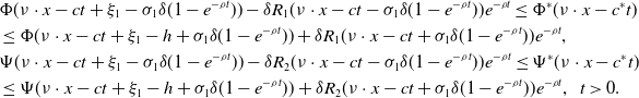 \begin{equation} \begin{aligned} &\Phi (\nu\ {\cdot}\ x-ct+\xi _1-\sigma _1\delta (1-e^{-\rho t}))-\delta R_1(\nu\ {\cdot}\ x-ct-\sigma _1\delta (1-e^{-\rho t}))e^{-\rho t}\le \Phi ^*(\nu\ {\cdot}\ x-c^*t)\\ &\le \Phi (\nu\ {\cdot}\ x-ct+\xi _1-h+\sigma _1\delta (1-e^{-\rho t}))+\delta R_1(\nu\ {\cdot}\ x-ct+\sigma _1\delta (1-e^{-\rho t}))e^{-\rho t},\\ &\Psi (\nu\ {\cdot}\ x-ct+\xi _1-\sigma _1\delta (1-e^{-\rho t}))-\delta R_2(\nu\ {\cdot}\ x-ct-\sigma _1\delta (1-e^{-\rho t}))e^{-\rho t}\le \Psi ^*(\nu\ {\cdot}\ x-c^*t)\\ &\le \Psi (\nu\ {\cdot}\ x-ct+\xi _1-h+\sigma _1\delta (1-e^{-\rho t}))+\delta R_2(\nu\ {\cdot}\ x-ct+\sigma _1\delta (1-e^{-\rho t}))e^{-\rho t}, \ \ t\gt 0. \end{aligned} \end{equation}
Fix $\bar{z}=\nu {\cdot}x-c^*t$
such that
$\bar{z}=\nu {\cdot}x-c^*t$
such that $\Phi ^*(\bar{z})\gt 0$
. If
$\Phi ^*(\bar{z})\gt 0$
. If $c^*\gt c$
, then
$c^*\gt c$
, then
 \begin{align*} \Phi ^*(\bar {z})\le \Phi (\bar {z}+(c^*-c))t+\xi _1-h+\sigma _1\delta (1-e^{-\rho t}))+\delta R_1(z+\sigma _1\delta (1-e^{-\rho t}))e^{-\rho t}\rightarrow 0, \text {as} \ t\rightarrow \infty . \end{align*}
It is in contradiction with the fact that $\Phi ^*(\bar{z})\gt 0$
, implying that
$\Phi ^*(\bar{z})\gt 0$
, implying that $c^* \leq c$
. Likewise, according to the left inequality in (2.35), we have
$c^* \leq c$
. Likewise, according to the left inequality in (2.35), we have $c^* \geq c$
. Consequently, we can conclude that
$c^* \geq c$
. Consequently, we can conclude that $c^* = c$
.
$c^* = c$
.
By taking the limit as $t\rightarrow \infty$
in (2.35), we obtain the following inequalities:
$t\rightarrow \infty$
in (2.35), we obtain the following inequalities:
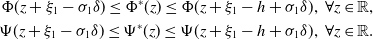 \begin{align*} \begin {aligned} \Phi (z+\xi _1-\sigma _1\delta )\le \Phi ^*(z)\le \Phi (z+\xi _1-h+\sigma _1\delta ), \ \forall z\in \mathbb {R},\\ \Psi (z+\xi _1-\sigma _1\delta )\le \Psi ^*(z)\le \Psi (z+\xi _1-h+\sigma _1\delta ), \ \forall z\in \mathbb {R}. \end {aligned} \end{align*}
Define
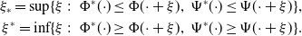 \begin{align*} \begin {aligned} \xi _*=\sup \{\xi \ :\ \ \Phi ^*({\cdot})\le \Phi ({\cdot}+\xi ), \ \Psi ^*({\cdot})\le \Psi ({\cdot}+\xi )\},\\ \xi ^*=\inf \{\xi \ :\ \ \Phi ^*({\cdot})\ge \Phi ({\cdot}+\xi ), \ \Psi ^*({\cdot})\ge \Psi ({\cdot}+\xi )\}. \end {aligned} \end{align*}
By employing a similar approach as the proof in [Reference Chen6, Theorem 2.1], we can prove $\xi _*=\xi ^*$
. Thus, the uniqueness of the wave profile, up to translation, is established.
$\xi _*=\xi ^*$
. Thus, the uniqueness of the wave profile, up to translation, is established.
The following theorem shows the monotonicity of bistable wave speed $c$
with respect to parameters
$c$
with respect to parameters $r$
and
$r$
and $b$
in the system (1.5)-(1.6).
$b$
in the system (1.5)-(1.6).
Theorem 2.9.
Assume that H1, (K1) and (K2) hold. For system (1.5)-(1.6), the bistable wave speed $c$
is non-increasing in
$c$
is non-increasing in $r$
when
$r$
when $b$
is fixed; The bistable wave speed
$b$
is fixed; The bistable wave speed $c$
is non-decreasing with respect to
$c$
is non-decreasing with respect to $b$
for fixed
$b$
for fixed $r$
.
$r$
.
Proof. We only prove that $c$
is non-increasing in
$c$
is non-increasing in $r$
. The monotonicity of
$r$
. The monotonicity of $c$
with respect to
$c$
with respect to $b$
can be proved by a similar method. Take
$b$
can be proved by a similar method. Take $0\lt r_1\le r_2$
. To the contrary, we assume
$0\lt r_1\le r_2$
. To the contrary, we assume $c_1\lt c_2$
, where
$c_1\lt c_2$
, where $c_i$
is the bistable wave speed when
$c_i$
is the bistable wave speed when $r=r_i, i=1,2$
. Let
$r=r_i, i=1,2$
. Let $(\Phi _i,\Psi _i)(z), i=1,2,$
be the travelling wave with speed
$(\Phi _i,\Psi _i)(z), i=1,2,$
be the travelling wave with speed $c_i$
, satisfying system (1.5)-(1.6). since
$c_i$
, satisfying system (1.5)-(1.6). since
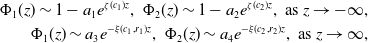 \begin{align*}\Phi _1(z)\sim 1-a_1e^{\zeta (c_1) z}, \ \Phi _2(z)\sim 1-a_2e^{\zeta (c_2) z},\ \text {as} \ z\rightarrow -\infty, \\ \Phi _1(z)\sim a_3e^{-\xi (c_1,r_1)z}, \ \Phi _2(z)\sim a_4e^{-\xi (c_2,r_2) z},\ \text {as} \ z\rightarrow \infty, \end{align*}
where $0\lt \zeta (c_2)\lt \zeta (c_1), 0\lt \xi (c_1,r_1)\lt \xi (c_2,r_2)$
and
$0\lt \zeta (c_2)\lt \zeta (c_1), 0\lt \xi (c_1,r_1)\lt \xi (c_2,r_2)$
and $a_i, i=1,2,3,4,$
are positive constants, and then by translation if necessary, we have
$a_i, i=1,2,3,4,$
are positive constants, and then by translation if necessary, we have $\Phi _2(\nu\ {\cdot}\ x)\le \Phi _1(\nu\ {\cdot}\ x)$
for all
$\Phi _2(\nu\ {\cdot}\ x)\le \Phi _1(\nu\ {\cdot}\ x)$
for all $x\in \mathbb{R}^n$
. By the
$x\in \mathbb{R}^n$
. By the $\Psi$
equation in system (1.5), we know
$\Psi$
equation in system (1.5), we know $(\Phi _2(\nu\ {\cdot}\ x),\Psi _2(\nu\ {\cdot}\ x))\le (\Phi _1(\nu\ {\cdot}\ x),\Psi _1(\nu\ {\cdot}\ x))$
for all
$(\Phi _2(\nu\ {\cdot}\ x),\Psi _2(\nu\ {\cdot}\ x))\le (\Phi _1(\nu\ {\cdot}\ x),\Psi _1(\nu\ {\cdot}\ x))$
for all $x\in \mathbb{R}^n$
. Using the comparison principle, we have
$x\in \mathbb{R}^n$
. Using the comparison principle, we have
 \begin{align*} \Phi _2(\nu\ {\cdot}\ x-c_2t)\le \Phi _1(\nu\ {\cdot}\ x-c_1t), \quad \Psi _2(\nu\ {\cdot}\ x-c_2t)\le \Psi _1(\nu\ {\cdot}\ x-c_1t). \end{align*}
Fix $z^*=\nu\ {\cdot}\ x-c_2t$
such that
$z^*=\nu\ {\cdot}\ x-c_2t$
such that $\Phi _2(z^*)\gt 0$
. It follows that
$\Phi _2(z^*)\gt 0$
. It follows that
 \begin{align*} \Phi _2(\nu\ {\cdot}\ x-c_2t) \le \Phi _1(\nu\ {\cdot}\ x-c_1t)=\Phi _1(z^*+(c_2-c_1)t)\rightarrow 0,\ \text {as}\ t\rightarrow \infty, \end{align*}
which contradicts $\Phi _2(z^*)\gt 0$
. Therefore,
$\Phi _2(z^*)\gt 0$
. Therefore, $c_1\ge c_2$
.
$c_1\ge c_2$
.
3. Travelling waves and speed selection in the case H2
In this section, we consider the monostable case H2, where $e_{\beta }$
is stable, and
$e_{\beta }$
is stable, and $e_0$
is unstable. Linearising (1.5) at
$e_0$
is unstable. Linearising (1.5) at $e_0$
, we derive the characteristic equation as
$e_0$
, we derive the characteristic equation as
 \begin{equation} \mu ^2-c\mu +(1-r)=0, \end{equation}
which yields two roots
 \begin{equation} \mu _1=\mu _1(c)=\frac{c-\sqrt{c^2-4(1-r)}}{2},\quad \mu _2=\mu _2(c)=\frac{c+\sqrt{c^2-4(1-r)}}{2}. \end{equation}
Denote $c_0=2\sqrt{1-r}$
as the linear speed so that
$c_0=2\sqrt{1-r}$
as the linear speed so that $\mu _1$
and
$\mu _1$
and $\mu _2$
are real when
$\mu _2$
are real when $c\ge c_0$
. Define
$c\ge c_0$
. Define $\bar{\mu }=\mu _1(c_0)=\mu _2(c_0)=\sqrt{1-r}$
.
$\bar{\mu }=\mu _1(c_0)=\mu _2(c_0)=\sqrt{1-r}$
.
3.1. Existence of monostable travelling waves
Before giving the existence of monostable monotone travelling waves of system (1.5)-(1.6), we first construct a lower solution for $c\gt c_0$
, which will be used in the proof of the subsequent theorem.
$c\gt c_0$
, which will be used in the proof of the subsequent theorem.
For any $c\gt c_0$
, define a continuous function
$c\gt c_0$
, define a continuous function
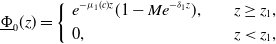 \begin{equation} \underline{\Phi }_0(z)=\left \{ \begin{array}{cc} \begin{aligned} &e^{-\mu _1(c) z} (1-Me^{-\delta _1 z}),\quad & z\geq z_1, \\ &0,\ &z\lt z_1,\\ \end{aligned} \end{array} \right . \end{equation}
where $0\lt \delta _1\ll 1$
,
$0\lt \delta _1\ll 1$
, $M$
is a positive constant to be determined, and
$M$
is a positive constant to be determined, and $z_1=\frac{\log M}{\delta _1}$
.
$z_1=\frac{\log M}{\delta _1}$
.
Lemma 3.1.
Assume that $r\in (0,1)$
and (K1) hold. If
$r\in (0,1)$
and (K1) hold. If $c=c_0+\delta _2$
and
$c=c_0+\delta _2$
and $\delta _2\gt 0$
, then
$\delta _2\gt 0$
, then $(\underline{\Phi }_0, \underline{\Psi }_0)(z)$
is a lower solution of system (1.5)-(1.6), where
$(\underline{\Phi }_0, \underline{\Psi }_0)(z)$
is a lower solution of system (1.5)-(1.6), where $\underline{\Phi }_0(z)$
is defined in (3.3), and
$\underline{\Phi }_0(z)$
is defined in (3.3), and $\underline{\Psi }_0(z)$
is the solution of the
$\underline{\Psi }_0(z)$
is the solution of the $\Psi$
-equation derived from the system using
$\Psi$
-equation derived from the system using $\Phi (z)=\underline{\Phi }_0(z)$
.
$\Phi (z)=\underline{\Phi }_0(z)$
.
Proof. Substituting $\underline{\Phi }_0(z)$
into
$\underline{\Phi }_0(z)$
into $\Phi$
-equation of (1.5), we obtain
$\Phi$
-equation of (1.5), we obtain
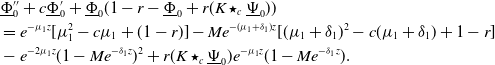 \begin{align*} \begin {aligned} &\underline {\Phi }_0^{\prime\prime}+c\underline {\Phi }_0^{\prime}+\underline {\Phi }_0(1-r-\underline {\Phi }_0+r(K\star _c\underline {\Psi }_0))\\ &=e^{-\mu _1 z}[\mu _1^2-c\mu _1+(1-r)]-Me^{-(\mu _1+\delta _1)z}[(\mu _1+\delta _1)^2-c(\mu _1+\delta _1)+1-r]\\ &-e^{-2\mu _1 z}(1-Me^{-\delta _1 z})^2+r(K\star _c\underline {\Psi }_0)e^{-\mu _1 z}(1-Me^{-\delta _1 z}). \end {aligned} \end{align*}
It is observed that the second term is positive. We can choose a sufficiently large $M$
such that the sum of the second and the third terms is positive. The first term is 0, and the last term is positive. Therefore, the proof is complete.
$M$
such that the sum of the second and the third terms is positive. The first term is 0, and the last term is positive. Therefore, the proof is complete.
In order to prove the existence of monostable monotone travelling waves of system (1.5)-(1.6) for the degenerate case $r=1$
, we introduce the following theorem.
$r=1$
, we introduce the following theorem.
Theorem 3.2.
Assume H2 and (K1) hold. If there exists a wavefront $(c_2,\Phi, \Psi )$
of (1.5)-(1.6),
$(c_2,\Phi, \Psi )$
of (1.5)-(1.6), $c_2\gt c_0$
such that
$c_2\gt c_0$
such that
 \begin{align*}\Phi (z)\sim A_2e^{-\mu _2(c_2) z},\ \text {as} \ z\rightarrow \infty, \ z=\nu {\cdot}x-c_2t,\ ||\nu ||=1,\end{align*}
with $A_2\gt 0$
, then
$A_2\gt 0$
, then $c_2=c_{\min }$
.
$c_2=c_{\min }$
.
Proof. we assume that there exists $c_2\gt c_0$
such that the travelling wave solution
$c_2\gt c_0$
such that the travelling wave solution $(\Phi (z), \Psi (z))$
satisfies
$(\Phi (z), \Psi (z))$
satisfies
 \begin{align*}\Phi (z)\sim A_2e^{-\mu _2(c_2) z},\ \text {as} \ z\rightarrow \infty, \ z=\nu {\cdot}x-c_2t,\end{align*}
with $A_2\gt 0$
. In this case, we claim that (1.5)-(1.6) have no travelling wave solutions for any
$A_2\gt 0$
. In this case, we claim that (1.5)-(1.6) have no travelling wave solutions for any $c\in [c_0, c_2)$
. To prove this by contradiction, assume that there exists
$c\in [c_0, c_2)$
. To prove this by contradiction, assume that there exists $\hat{c}\in (c_0,c_2)$
for which the system (1.2) has a decreasing travelling wave solution
$\hat{c}\in (c_0,c_2)$
for which the system (1.2) has a decreasing travelling wave solution $(\bar{\Phi },\bar{\Psi })(\nu\ {\cdot}\ x-\hat{c}t)$
with initial conditions
$(\bar{\Phi },\bar{\Psi })(\nu\ {\cdot}\ x-\hat{c}t)$
with initial conditions
 \begin{align*} \phi (0,x)=\bar {\Phi }(\nu\ {\cdot}\ x) \quad \text {and} \quad \psi (0,x)=\bar {\Psi }(\nu\ {\cdot}\ x). \end{align*}
Clearly, $(\bar{\Phi },\bar{\Psi })(z)$
satisfies system (1.5) with
$(\bar{\Phi },\bar{\Psi })(z)$
satisfies system (1.5) with $c=\hat{c}$
. Since
$c=\hat{c}$
. Since $\mu _2(c)$
is non-decreasing with respect to
$\mu _2(c)$
is non-decreasing with respect to $c$
, we get
$c$
, we get $\mu _1(\hat{c})\le \mu _2(\hat{c})\le \mu _2(c_2)$
. Recall that
$\mu _1(\hat{c})\le \mu _2(\hat{c})\le \mu _2(c_2)$
. Recall that $\Phi (z)\sim A_2 e^{-\mu _2(c_2) z}$
as
$\Phi (z)\sim A_2 e^{-\mu _2(c_2) z}$
as $z\rightarrow \infty$
. It follows that
$z\rightarrow \infty$
. It follows that $\Phi (z)\le \bar{\Phi }(z)$
as
$\Phi (z)\le \bar{\Phi }(z)$
as $z\rightarrow \infty$
. Note that
$z\rightarrow \infty$
. Note that $\Phi (z)\sim 1-A_3e^{\gamma z}$
as
$\Phi (z)\sim 1-A_3e^{\gamma z}$
as $z\rightarrow -\infty$
for positive
$z\rightarrow -\infty$
for positive $A_3$
and
$A_3$
and $\gamma$
, and
$\gamma$
, and $\gamma$
is non-increasing with respect to
$\gamma$
is non-increasing with respect to $c$
. Therefore,
$c$
. Therefore, $\Phi (z)\le \bar{\Phi }(z)$
as
$\Phi (z)\le \bar{\Phi }(z)$
as $z\rightarrow -\infty$
. Making a translation if necessary, we can always ensure that
$z\rightarrow -\infty$
. Making a translation if necessary, we can always ensure that $\Phi (z)\le \bar{\Phi }(z)$
for all
$\Phi (z)\le \bar{\Phi }(z)$
for all $z$
. Considering the second equation of (1.2), we then have
$z$
. Considering the second equation of (1.2), we then have $(\Phi, \Psi )(\nu\ {\cdot}\ x)\le (\bar{\Phi },\bar{\Psi })(\nu\ {\cdot}\ x)$
for all
$(\Phi, \Psi )(\nu\ {\cdot}\ x)\le (\bar{\Phi },\bar{\Psi })(\nu\ {\cdot}\ x)$
for all $x\in \mathbb{R}^n$
(by shift if necessary). By comparison, it gives that
$x\in \mathbb{R}^n$
(by shift if necessary). By comparison, it gives that
 \begin{equation} \Phi (\nu\ {\cdot}\ x-c_2t)\le \bar{\Phi }(\nu\ {\cdot}\ x-\hat{c}t). \end{equation}
Fix $\hat{z}=\nu\ {\cdot}\ x-c_2t$
such that
$\hat{z}=\nu\ {\cdot}\ x-c_2t$
such that $\Phi (\hat{z})\gt 0$
. Observe that
$\Phi (\hat{z})\gt 0$
. Observe that
 \begin{align*} \bar {\Phi }(\nu\ {\cdot}\ x-\hat {c}t)=\bar {\Phi }(\hat {z}+(c_2-\hat {c})t))\rightarrow 0, \quad \text {as}\quad t \rightarrow \infty . \end{align*}
Thus, we obtain
 \begin{align*} \Phi (\hat {z})\le \bar {\Phi }(\nu\ {\cdot}\ x-\hat {c}t)\rightarrow 0, \quad \text {as}\quad t \rightarrow \infty, \end{align*}
which contradicts the fact $\Phi (\hat{z})\gt 0$
. Therefore, there is no travelling wave solution of system (1.5)-(1.6) for any
$\Phi (\hat{z})\gt 0$
. Therefore, there is no travelling wave solution of system (1.5)-(1.6) for any $\hat{c}\in (c_0,c_2)$
. When
$\hat{c}\in (c_0,c_2)$
. When $r\in (0,1)$
, if
$r\in (0,1)$
, if $\hat{c}=c_0$
in our assumption, then the travelling waves exist if and only if
$\hat{c}=c_0$
in our assumption, then the travelling waves exist if and only if $\hat{c}\ge c_0$
[Reference Hasík, Kopfová, Nábělková, Trofymchuk and Trofimchuk12, Theorem 5]. We can still derive a contradiction by the above argument. If
$\hat{c}\ge c_0$
[Reference Hasík, Kopfová, Nábělková, Trofymchuk and Trofimchuk12, Theorem 5]. We can still derive a contradiction by the above argument. If $r=1$
, then
$r=1$
, then $c_0=0$
. The second equation of (1.5) and the boundary condition (1.6) mean
$c_0=0$
. The second equation of (1.5) and the boundary condition (1.6) mean $\hat{c}\gt c_0$
. Therefore, the proof is complete.
$\hat{c}\gt c_0$
. Therefore, the proof is complete.
The existence of monostable monotone travelling waves of system (1.5)-(1.6) is established in the theorem below.
Theorem 3.3.
Assume that H2 and (K1) hold. There is a finite $c_{\min }\ge c_0$
such that monotone and positive travelling wave solutions of (1.5)-(1.6) exist if and only if
$c_{\min }\ge c_0$
such that monotone and positive travelling wave solutions of (1.5)-(1.6) exist if and only if $c\ge c_{\min }$
. Here
$c\ge c_{\min }$
. Here $c_{\min }$
is non-increasing with respect to
$c_{\min }$
is non-increasing with respect to $r$
. Furthermore, when
$r$
. Furthermore, when $r=1$
, the travelling wave solution
$r=1$
, the travelling wave solution $(\Phi, \Psi )(z)$
of (1.5)-(1.6) with speed
$(\Phi, \Psi )(z)$
of (1.5)-(1.6) with speed $c\gt c_{\min }$
has the following algebraic decay behaviour
$c\gt c_{\min }$
has the following algebraic decay behaviour
 \begin{align*} \Phi (z) \sim \frac {2c^2}{b} z^{-2}, \ \ \Psi (z) \sim 2c z^{-1}, \ \ \text {as} \ \ z\rightarrow \infty . \end{align*}
Proof. When $r\lt 1$
, the existence of the minimal wave speed
$r\lt 1$
, the existence of the minimal wave speed $c_{\min }$
, ensuring that monotone and positive travelling wave solutions of (1.5)-(1.6) exist if and only if
$c_{\min }$
, ensuring that monotone and positive travelling wave solutions of (1.5)-(1.6) exist if and only if $c\ge c_{\min }$
, is guaranteed by [Reference Hasík, Kopfová, Nábělková, Trofymchuk and Trofimchuk12, Theorem 5]. We claim that
$c\ge c_{\min }$
, is guaranteed by [Reference Hasík, Kopfová, Nábělková, Trofymchuk and Trofimchuk12, Theorem 5]. We claim that $c_{\min }$
is non-increasing with respect to
$c_{\min }$
is non-increasing with respect to $r$
. Indeed, let
$r$
. Indeed, let $r_a\lt r_b\lt 1$
. There exists the minimal-speed travelling wave solution
$r_a\lt r_b\lt 1$
. There exists the minimal-speed travelling wave solution $(c_{\min }^{r_a}, \Phi ^{r_a}(z))$
satisfying system (2.2) with
$(c_{\min }^{r_a}, \Phi ^{r_a}(z))$
satisfying system (2.2) with $r=r_a$
(here,
$r=r_a$
(here, $c_{\min }^{r_a}$
represents the minimal wave speed when
$c_{\min }^{r_a}$
represents the minimal wave speed when $r=r_a$
). Note that
$r=r_a$
). Note that $(c_{\min }^{r_a}, \Phi ^{r_a}(z))$
is an upper solution of the system with
$(c_{\min }^{r_a}, \Phi ^{r_a}(z))$
is an upper solution of the system with $r=r_b$
. A lower solution is defined as in (3.3). Then there exists a travelling wave solution of the system for
$r=r_b$
. A lower solution is defined as in (3.3). Then there exists a travelling wave solution of the system for $r=r_b$
when
$r=r_b$
when $c=c_{\min }^{r_a}$
. It follows that
$c=c_{\min }^{r_a}$
. It follows that $c_{\min }^{r_b}\le c_{\min }^{r_a}$
. Therefore,
$c_{\min }^{r_b}\le c_{\min }^{r_a}$
. Therefore, $c_{\min }^{r}$
is non-increasing with respect to
$c_{\min }^{r}$
is non-increasing with respect to $r$
.
$r$
.
For the existence of monotone travelling wave solutions of (1.5)-(1.6) when $r=1$
, we divide the proof into four steps.
$r=1$
, we divide the proof into four steps.
Step 1. In this step, we shall prove that when $r=1$
, there exists a minimal speed so that (1.5)-(1.6) has a monotone travelling wave solution. Take a decreasing real sequence
$r=1$
, there exists a minimal speed so that (1.5)-(1.6) has a monotone travelling wave solution. Take a decreasing real sequence $\{r_n\}$
such that
$\{r_n\}$
such that $\lim \limits _{n\rightarrow \infty }r_n=\bar{r}=1$
and
$\lim \limits _{n\rightarrow \infty }r_n=\bar{r}=1$
and $r_0=2$
. By Theorem2.6, for each
$r_0=2$
. By Theorem2.6, for each $r_n$
, there exists monotone travelling wave
$r_n$
, there exists monotone travelling wave $(c^{r_n}, \Phi ^{r_n}(z))$
of (2.2) with
$(c^{r_n}, \Phi ^{r_n}(z))$
of (2.2) with $r=r_n$
(here,
$r=r_n$
(here, $c^{r_n}$
represents the unique positive bistable wave speed when
$c^{r_n}$
represents the unique positive bistable wave speed when $r=r_n$
), and
$r=r_n$
), and $\Psi ^{r_n}(z)=\mathcal{L}_{b,c^{r_n}}\Phi ^{r_n}(z)$
. By shifting, we can choose a large
$\Psi ^{r_n}(z)=\mathcal{L}_{b,c^{r_n}}\Phi ^{r_n}(z)$
. By shifting, we can choose a large $L_1\gt 0$
to fix
$L_1\gt 0$
to fix $\Phi ^{r_n}(L_1)=\epsilon _1$
for each
$\Phi ^{r_n}(L_1)=\epsilon _1$
for each $n$
, where
$n$
, where $\epsilon _1$
is sufficiently small.
$\epsilon _1$
is sufficiently small.
Claim 1: The bistable wave speeds $c^{r_n}$
have a finite upper bound.
$c^{r_n}$
have a finite upper bound.
Let $\hat{r}=0.5$
. Assume that
$\hat{r}=0.5$
. Assume that $\Phi ^{\hat{r}}(z)$
is a travelling wave of (2.2) with speed
$\Phi ^{\hat{r}}(z)$
is a travelling wave of (2.2) with speed $c=c_1=2c_{\min }^{\hat{r}}$
and
$c=c_1=2c_{\min }^{\hat{r}}$
and $r=\hat{r}$
, where
$r=\hat{r}$
, where $c_{\min }^{\hat{r}}$
represents the minimal wave speed when
$c_{\min }^{\hat{r}}$
represents the minimal wave speed when $r=\hat{r}$
. We shall prove
$r=\hat{r}$
. We shall prove $c^{r_n}\le c_1$
for all
$c^{r_n}\le c_1$
for all $n\in \mathbb{N}^+$
. To the contrary, assume there exists
$n\in \mathbb{N}^+$
. To the contrary, assume there exists $j\in \mathbb{N}^+$
such that
$j\in \mathbb{N}^+$
such that $c_2\,:\!=\,c^{r_j}\gt c_1$
. By asymptotic analysis, we have
$c_2\,:\!=\,c^{r_j}\gt c_1$
. By asymptotic analysis, we have
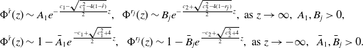 \begin{equation} \begin{aligned} &\Phi ^{\hat{r}}(z) \sim A_1 e^{-\frac{c_1-\sqrt{c_1^2-4(1-\hat{r})}}{2} z}, \ \ \Phi ^{r_j}(z) \sim B_j e^{-\frac{c_2+\sqrt{c_2^2-4(1-r_j)}}{2} z}, \ \text{as} \ z\rightarrow \infty, \ A_1,B_j\gt 0, \\ &\Phi ^{\hat{r}}(z) \sim 1-\bar{A}_1 e^{\frac{-c_1+\sqrt{c_1^2+4}}{2} z}, \ \ \Phi ^{r_j}(z) \sim 1-\bar{B}_j e^{\frac{-c_2+\sqrt{c_2^2+4}}{2} z}, \ \text{as} \ z\rightarrow -\infty, \ \ \bar{A}_1, \bar{B}_j\gt 0. \end{aligned} \end{equation}
Thus, by translation if necessary, we obtain $\Phi ^{\hat{r}}(\nu\ {\cdot}\ x)\ge \Phi ^{r_j}(\nu\ {\cdot}\ x)$
for
$\Phi ^{\hat{r}}(\nu\ {\cdot}\ x)\ge \Phi ^{r_j}(\nu\ {\cdot}\ x)$
for $x\in \mathbb{R}^n$
. A similar argument as in Theorem2.9 leads to a contradiction. It means
$x\in \mathbb{R}^n$
. A similar argument as in Theorem2.9 leads to a contradiction. It means $c^{r_n}\le c_1$
for all
$c^{r_n}\le c_1$
for all $n\in \mathbb{N}^+$
.
$n\in \mathbb{N}^+$
.
Since $c^{r_n}$
is non-increasing with respect to
$c^{r_n}$
is non-increasing with respect to $r_n$
as stated in Theorem2.9, we know
$r_n$
as stated in Theorem2.9, we know $c^{r_n}$
is non-decreasing with respect to
$c^{r_n}$
is non-decreasing with respect to $n$
. Together with Claim 1, we conclude that
$n$
. Together with Claim 1, we conclude that $c^{r_n}$
has a limit when
$c^{r_n}$
has a limit when $n\rightarrow \infty$
, denoted by
$n\rightarrow \infty$
, denoted by $c^{\bar{r}}$
. Let
$c^{\bar{r}}$
. Let $\bar{\alpha }$
be large enough so that
$\bar{\alpha }$
be large enough so that
 \begin{align*} \bar {F}(\Phi )\,:\!=\,\bar {\alpha }\Phi +\Phi (1-r-\Phi +r(K\star _c\mathcal {L}_{b,c}\Phi )) \end{align*}
is non-decreasing in $\Phi$
. Then we can express
$\Phi$
. Then we can express $\Phi$
-equation in (2.2) as
$\Phi$
-equation in (2.2) as
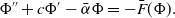 \begin{equation} \begin{aligned} \Phi ^{\prime\prime}+c\Phi ^{\prime}-\bar{\alpha } \Phi =-\bar{F}(\Phi ).\\ \end{aligned} \end{equation}
Define $\bar{\beta }_1$
and
$\bar{\beta }_1$
and $\bar{\beta }_2$
as
$\bar{\beta }_2$
as
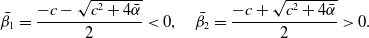 \begin{equation} \bar{\beta }_1=\frac{-c-\sqrt{c^2+4\bar{\alpha }}}{2}\lt 0, \quad \bar{\beta }_2=\frac{-c+\sqrt{c^2+4\bar{\alpha }}}{2}\gt 0. \end{equation}
Then, the integral form of (3.6) is
 \begin{equation} \begin{aligned} \Phi (z)=\frac{1}{\bar{\beta }_2-\bar{\beta }_1}\bigg \{\int _{-\infty }^{z}e^{\bar{\beta }_1(z-t)}\bar{F}(\Phi )(t)dt+\int _{z}^{\infty }e^{\bar{\beta }_2(z-t)}\bar{F}(\Phi )(t)dt\bigg \}. \end{aligned} \end{equation}
Note that $(c^{r_n}, \Phi ^{r_n}(z))$
satisfies the integral system (3.8). Then we have
$(c^{r_n}, \Phi ^{r_n}(z))$
satisfies the integral system (3.8). Then we have
 \begin{align*} \begin{aligned} &\bigg |\frac{d\Phi ^{r_n}(z)}{dz}\bigg |\le \frac{\beta _2}{\beta _2-\beta _1}\bigg |\bigg \{\int _{-\infty }^{z}e^{\beta _1(z-t)}\bar F(\Phi )(t)dt+\int _{z}^{\infty }e^{\beta _2(z-t)}\bar F(\Phi )(t)dt\bigg \}\bigg |\le \beta _2\lt \infty, \\ \end{aligned} \end{align*}
which means $(\Phi ^{r_n}(z))$
is equicontinuous and uniformly bounded. According to the Ascoli–Arzela theorem, there exists a subsequence
$(\Phi ^{r_n}(z))$
is equicontinuous and uniformly bounded. According to the Ascoli–Arzela theorem, there exists a subsequence $\{r_{n_j}\}$
such that
$\{r_{n_j}\}$
such that $(c^{r_{n_j}}, \Phi ^{r_{n_j}}(z))$
converges to a limit
$(c^{r_{n_j}}, \Phi ^{r_{n_j}}(z))$
converges to a limit $(c^{\bar{r}}, \Phi ^{\bar{r}}(z))$
uniformly on any compact interval and pointwise on
$(c^{\bar{r}}, \Phi ^{\bar{r}}(z))$
uniformly on any compact interval and pointwise on $\mathbb{R}$
. Take
$\mathbb{R}$
. Take $\bar{\lambda }\,:\!=\,\inf _{n\in \mathbb{N}^+} \{\frac{c^{r_n}+\sqrt{(c^{r_n})^2-4(1-r_n)}}{2}\}\gt 0$
. Since
$\bar{\lambda }\,:\!=\,\inf _{n\in \mathbb{N}^+} \{\frac{c^{r_n}+\sqrt{(c^{r_n})^2-4(1-r_n)}}{2}\}\gt 0$
. Since $\epsilon _1$
is sufficiently small, and by the asymptotic behaviour as in (3.5), we have
$\epsilon _1$
is sufficiently small, and by the asymptotic behaviour as in (3.5), we have $\Phi ^{r_n}(z)\le \epsilon _1 e^{-\bar{\lambda } (z-L_1)}$
when
$\Phi ^{r_n}(z)\le \epsilon _1 e^{-\bar{\lambda } (z-L_1)}$
when $z\ge L_1$
. It follows that
$z\ge L_1$
. It follows that
 \begin{equation} \Phi ^{\bar{r}}(z)\le \epsilon _1 e^{-\bar{\lambda } (z-L_1)}, \ \text{when}\ \ z\ge L_1, \end{equation}
which means $\int _{0}^{\infty }\Phi ^{\bar{r}}(z)dz$
is finite. Let
$\int _{0}^{\infty }\Phi ^{\bar{r}}(z)dz$
is finite. Let $j\rightarrow \infty$
. By the dominated converges theorem, we know
$j\rightarrow \infty$
. By the dominated converges theorem, we know $(c^{\bar{r}}, \Phi ^{\bar{r}}(z))$
satisfies the integral system (3.8) and
$(c^{\bar{r}}, \Phi ^{\bar{r}}(z))$
satisfies the integral system (3.8) and $\Psi ^{\bar{r}}(z)=\mathcal{L}_{b,c^{\bar{r}}}\Phi ^{\bar{r}}(z)$
. Using the monotone convergence theorem, we know
$\Psi ^{\bar{r}}(z)=\mathcal{L}_{b,c^{\bar{r}}}\Phi ^{\bar{r}}(z)$
. Using the monotone convergence theorem, we know $(c^{\bar{r}}, \Phi ^{\bar{r}}(\pm \infty ))$
satisfy system (3.8). Therefore,
$(c^{\bar{r}}, \Phi ^{\bar{r}}(\pm \infty ))$
satisfy system (3.8). Therefore, $\Phi ^{\bar{r}}({-}\infty )=1$
and
$\Phi ^{\bar{r}}({-}\infty )=1$
and $\Phi ^{\bar{r}}(\infty )=0$
. By Lemma 2.1, we have
$\Phi ^{\bar{r}}(\infty )=0$
. By Lemma 2.1, we have $\Psi ^{\bar{r}}({-}\infty )=1$
and
$\Psi ^{\bar{r}}({-}\infty )=1$
and $\Psi ^{\bar{r}}(\infty )=0$
. Notice that
$\Psi ^{\bar{r}}(\infty )=0$
. Notice that $\mu _1=0$
when
$\mu _1=0$
when $r=\bar{r}=1$
. Thus, inequality (3.9) shows that
$r=\bar{r}=1$
. Thus, inequality (3.9) shows that $\Phi ^{\bar{r}}(z)$
decays exponentially to
$\Phi ^{\bar{r}}(z)$
decays exponentially to $0$
with decay rate
$0$
with decay rate $\mu _2(c^{\bar{r}})$
, as
$\mu _2(c^{\bar{r}})$
, as $z\rightarrow \infty$
. It follows from Theorem3.2 that
$z\rightarrow \infty$
. It follows from Theorem3.2 that $c^{\bar{r}}$
is the minimal speed when
$c^{\bar{r}}$
is the minimal speed when $r=1$
, that is,
$r=1$
, that is, $c_{\min }^{\bar{r}}=c^{\bar{r}}$
.
$c_{\min }^{\bar{r}}=c^{\bar{r}}$
.
Step 2. In this step, we aim to prove the existence of monostable monotone travelling waves of system (1.5)-(1.6) with $r=1$
when
$r=1$
when $c$
is sufficiently large. By letting
$c$
is sufficiently large. By letting
 \begin{align*} \tilde {z}=c z, \ \ \ \ \tilde {\Phi }(\tilde {z})=\Phi (z), \ \ \ \ \tilde {\Psi }(\tilde {z})=\Psi (z), \end{align*}
system (1.5)-(1.6) can be transformed into
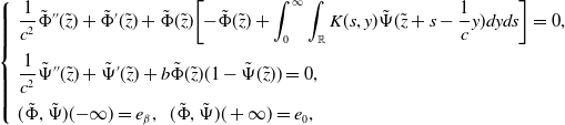 \begin{equation} \left \{ \begin{array}{cc} \begin{aligned} &\frac{1}{c^2}\tilde{\Phi }^{\prime\prime}(\tilde{z})+\tilde{\Phi }^{\prime}(\tilde{z})+\tilde{\Phi }(\tilde{z})\bigg [{-}\tilde{\Phi }(\tilde{z})+\int _{0}^{\infty }\int _{\mathbb{R}} K(s,y)\tilde{\Psi }(\tilde{z}+s-\frac{1}{c}y)dyds\bigg ] =0, \\[3pt] &\frac{1}{c^2}\tilde{\Psi }^{\prime\prime}(\tilde{z})+\tilde{\Psi }^{\prime}(\tilde{z})+b\tilde{\Phi }(\tilde{z})(1-\tilde{\Psi }(\tilde{z}))=0, \\[3pt] &(\tilde{\Phi }, \tilde{\Psi })({-}\infty )=e_\beta, \ \ (\tilde{\Phi }, \tilde{\Psi })(+\infty )=e_0, \end{aligned} \end{array}\right . \end{equation}
when $r=1$
. Let
$r=1$
. Let $c=\frac{1}{\varepsilon }$
, where
$c=\frac{1}{\varepsilon }$
, where $\varepsilon$
is small enough. We first consider
$\varepsilon$
is small enough. We first consider
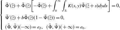 \begin{equation} \left \{ \begin{array}{cc} \begin{aligned} &\tilde{\Phi }^{\prime}(\tilde{z})+\tilde{\Phi }(\tilde{z})\bigg [{-}\tilde{\Phi }(\tilde{z})+\int _{0}^{\infty }\int _{\mathbb{R}} K(s,y)\tilde{\Psi }(\tilde{z}+s)dyds\bigg ] =0, \\[3pt] &\tilde{\Psi }^{\prime}(\tilde{z})+b\tilde{\Phi }(\tilde{z})(1-\tilde{\Psi }(\tilde{z}))=0, \\[3pt] &(\tilde{\Phi }, \tilde{\Psi })({-}\infty )=e_\beta, \ \ (\tilde{\Phi }, \tilde{\Psi })(+\infty )=e_0. \end{aligned} \end{array}\right . \end{equation}
From the second equation in (3.11) and $(\tilde{\Phi }, \tilde{\Psi })({+}\infty )=e_0$
, we have
$(\tilde{\Phi }, \tilde{\Psi })({+}\infty )=e_0$
, we have
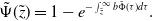 \begin{align*} \tilde {\Psi }(\tilde {z})=1-e^{-\int _{\tilde {z}}^{\infty }b\tilde {\Phi }(\tau )d\tau }. \end{align*}
Thus, system (3.11) becomes
 \begin{equation} \tilde{\Phi }^{\prime}(\tilde{z})+\tilde{\Phi }(\tilde{z})\bigg [{-}\tilde{\Phi }(\tilde{z})+\int _{0}^{\infty }\int _{\mathbb{R}} K(s,y)(1-e^{-\int _{\tilde{z}+s}^{\infty }b\tilde{\Phi }(\tau )d\tau })dyds\bigg ] =0 \end{equation}
with the boundary condition
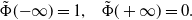 \begin{equation} \tilde{\Phi }({-}\infty )=1, \ \ \ \tilde{\Phi }(+\infty )=0. \end{equation}
The integral form of (3.12) is
 \begin{align*} \tilde {T}_1(\tilde {\Phi })=\int _{\tilde {z}}^{\infty }e^{4(\tilde {z}-\tau _1)}\tilde {\Phi }(\tau _1)\bigg [4-\tilde {\Phi }(\tau _1)+\int _{0}^{\infty }\int _{\mathbb {R}} K(s,y)(1-e^{-\int _{\tau _1+s}^{\infty }b\tilde {\Phi }(\tau )d\tau })dyds\bigg ] d\tau _1. \end{align*}
By calculation, we can establish $\int _{0}^{\infty } \tilde{T}_1(\tilde{\Phi })(\tilde{z})d\tilde{z}$
is finite when
$\int _{0}^{\infty } \tilde{T}_1(\tilde{\Phi })(\tilde{z})d\tilde{z}$
is finite when $\tilde{\Phi }(\tilde{z}) \in L^1[0,\infty )$
. Note that
$\tilde{\Phi }(\tilde{z}) \in L^1[0,\infty )$
. Note that $\tilde{T}_1$
has only two fixed points
$\tilde{T}_1$
has only two fixed points $0$
and
$0$
and $1$
. Then
$1$
. Then $\tilde{T}_1\ :\ \mathcal{M}_\beta \cap L^1[0,\infty )\rightarrow \mathcal{M}_\beta \cap L^1[0,\infty )$
, where
$\tilde{T}_1\ :\ \mathcal{M}_\beta \cap L^1[0,\infty )\rightarrow \mathcal{M}_\beta \cap L^1[0,\infty )$
, where $\mathcal{M}_\beta$
is defined in Section 2 with
$\mathcal{M}_\beta$
is defined in Section 2 with $\beta =1$
, is a strictly monotone continuous operator. By the Dancer–Hess Lemma (see [Reference Dancer and Hess7, Proposition 1], [Reference Zhao45, p. 45]), there exists an entire orbit of
$\beta =1$
, is a strictly monotone continuous operator. By the Dancer–Hess Lemma (see [Reference Dancer and Hess7, Proposition 1], [Reference Zhao45, p. 45]), there exists an entire orbit of $\tilde{T}_1$
connecting
$\tilde{T}_1$
connecting $1$
to
$1$
to $0$
. Therefore, system (3.12)-(3.13) has a monotone solution, denoted by
$0$
. Therefore, system (3.12)-(3.13) has a monotone solution, denoted by $\tilde{\Phi }_1(\tilde{z})$
. From (3.12),
$\tilde{\Phi }_1(\tilde{z})$
. From (3.12), $\tilde{\Phi }_1(\tilde{z})$
does not decay exponentially to
$\tilde{\Phi }_1(\tilde{z})$
does not decay exponentially to $0$
as
$0$
as $z\rightarrow \infty$
. Consider
$z\rightarrow \infty$
. Consider $z\rightarrow \infty$
. We let
$z\rightarrow \infty$
. We let
 \begin{equation} \tilde{\Phi }_1(\tilde{z})=a_1 \tilde{z}^{-\gamma }+o(\tilde{z}^{-\gamma }), \ \ \ \ a_1, \gamma \gt 0. \end{equation}
Substituting (3.14) into (3.12) yields
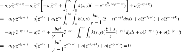 \begin{equation} \begin{aligned} &-a_1\gamma \tilde{z}^{-(\gamma +1)}+a_1 \tilde{z}^{-\gamma }\bigg [{-}a_1 \tilde{z}^{-\gamma }+ \int _{0}^{\infty }\int _{\mathbb{R}} k(s, y) (1-e^{-\int _{\tilde{z}+s}^{\infty }ba_1\tau ^{-\gamma } d\tau })\bigg ]+o(\tilde{z}^{-(\gamma +1)}) \\ &=-a_1\gamma \tilde{z}^{-(\gamma +1)}-a_1^2 \tilde{z}^{-2\gamma }+a_1 \tilde{z}^{-\gamma }\int _{0}^{\infty }\int _{\mathbb{R}} k(s, y)\frac{ba_1}{\gamma -1}(\tilde{z}+s)^{-\gamma +1} dyds+o(\tilde{z}^{-2\gamma +1}) +o(\tilde{z}^{-(\gamma +1)})\\ &=-a_1\gamma \tilde{z}^{-(\gamma +1)}-a_1^2 \tilde{z}^{-2\gamma }+\frac{ba_1^2}{\gamma -1} \tilde{z}^{-2\gamma +1}\int _{0}^{\infty }\int _{\mathbb{R}} k(s, y)(\frac{\tilde{z}+s}{\tilde{z}})^{-\gamma +1} dyds+o(\tilde{z}^{-2\gamma +1}) +o(\tilde{z}^{-(\gamma +1)}) \\ &=-a_1\gamma \tilde{z}^{-(\gamma +1)}-a_1^2 \tilde{z}^{-2\gamma }+\frac{ba_1^2}{\gamma -1} \tilde{z}^{-2\gamma +1}+o(\tilde{z}^{-2\gamma +1})+o(\tilde{z}^{-(\gamma +1)}) =0. \end{aligned} \end{equation}
According to the leading terms in (3.15), we derive that $\gamma =2$
and
$\gamma =2$
and $a_1=\frac{2}{b}$
. Therefore, system (3.11) has a monotone solution
$a_1=\frac{2}{b}$
. Therefore, system (3.11) has a monotone solution $(\tilde{\Phi }_1, \tilde{\Psi }_1)(\tilde{z})$
, where
$(\tilde{\Phi }_1, \tilde{\Psi }_1)(\tilde{z})$
, where $\tilde{\Psi }_1(\tilde{z})=1-e^{-\int _{\tilde{z}}^{\infty }b\tilde{\Phi }_1(\tau )d\tau }$
, with decay behaviour
$\tilde{\Psi }_1(\tilde{z})=1-e^{-\int _{\tilde{z}}^{\infty }b\tilde{\Phi }_1(\tau )d\tau }$
, with decay behaviour
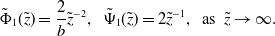 \begin{equation} \tilde{\Phi }_1(\tilde{z})=\frac{2}{b} \tilde{z}^{-2}, \ \ \tilde{\Psi }_1(\tilde{z})=2\tilde{z}^{-1}, \ \ \text{as} \ \ \tilde{z}\rightarrow \infty . \end{equation}
From (3.11), we know $\tilde{\Phi }^{\prime\prime}_1$
and
$\tilde{\Phi }^{\prime\prime}_1$
and $\tilde{\Psi }^{\prime\prime}_1$
are smooth. Next, we want to apply a perturbation argument to prove that solutions of (3.10) exist for large speed
$\tilde{\Psi }^{\prime\prime}_1$
are smooth. Next, we want to apply a perturbation argument to prove that solutions of (3.10) exist for large speed $c$
by using
$c$
by using $(\tilde{\Phi }_1, \tilde{\Psi }_1)$
. Let
$(\tilde{\Phi }_1, \tilde{\Psi }_1)$
. Let $\tilde{\alpha }_1$
be large enough so that
$\tilde{\alpha }_1$
be large enough so that
 \begin{align*} F_3(\tilde {\Phi }, \tilde {\Psi })\,:\!=\,\tilde {\alpha }_1 \tilde {\Phi }+\tilde {\Phi }(\tilde {z})\bigg [{-}\tilde {\Phi }(\tilde {z})+\int _{0}^{\infty }\int _{\mathbb {R}} K(s,y)\tilde {\Psi }(\tilde {z}+s-\frac {1}{c}y)dyds\bigg ] \end{align*}
and
 \begin{align*} F_4(\tilde {\Phi }, \tilde {\Psi })\,:\!=\,\tilde {\alpha }_1 \tilde {\Psi }+b\tilde {\Phi }(\tilde {z})(1-\tilde {\Psi }(\tilde {z})) \end{align*}
are non-decreasing functions of $\tilde{\Phi }$
and
$\tilde{\Phi }$
and $\tilde{\Psi }$
. Then we can write system (3.10) as
$\tilde{\Psi }$
. Then we can write system (3.10) as
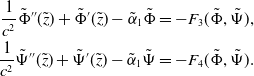 \begin{equation} \begin{aligned} \frac{1}{c^2}\tilde{\Phi }^{\prime\prime}(\tilde{z})+\tilde{\Phi }^{\prime}(\tilde{z})-\tilde{\alpha }_1 \tilde{\Phi }=-F_3(\tilde{\Phi }, \tilde{\Psi }),\\ \frac{1}{c^2}\tilde{\Psi }^{\prime\prime}(\tilde{z})+\tilde{\Psi }^{\prime}(\tilde{z})-\tilde{\alpha }_1 \tilde{\Psi }=-F_4(\tilde{\Phi }, \tilde{\Psi }).\\ \end{aligned} \end{equation}
Define $\tilde{\beta }_1$
and
$\tilde{\beta }_1$
and $\tilde{\beta }_2$
as
$\tilde{\beta }_2$
as
 \begin{equation} \tilde{\beta }_1(c)=\frac{-c^2-c\sqrt{c^2+4\tilde{\alpha }_1}}{2}\lt 0, \quad \tilde{\beta }_2(c)=\frac{-c^2+c\sqrt{c^2+4\tilde{\alpha }_1}}{2}\gt 0. \end{equation}
The integral form of (3.17) is
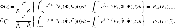 \begin{equation} \begin{aligned} \tilde{\Phi }(\tilde{z})=\frac{c^2}{\tilde{\beta }_2-\tilde{\beta }_1}\bigg \{\int _{-\infty }^{\tilde{z}}e^{\tilde{\beta }_1(\tilde{z}-t)}F_3(\tilde{\Phi },\tilde{\Psi })(t)dt+\int _{\tilde{z}}^{\infty }e^{\tilde{\beta }_2(\tilde{z}-t)}F_3(\tilde{\Phi }, \tilde{\Psi })(t)dt\bigg \} \,=\!:\,P_{1,c}(F_3)(\tilde{z}),\\ \tilde{\Psi }(\tilde{z})=\frac{c^2}{\tilde{\beta }_2-\tilde{\beta }_1}\bigg \{\int _{-\infty }^{\tilde{z}}e^{\tilde{\beta }_1(\tilde{z}-t)}F_4(\tilde{\Phi },\tilde{\Psi })(t)dt+\int _{\tilde{z}}^{\infty }e^{\tilde{\beta }_2(\tilde{z}-t)}F_4(\tilde{\Phi }, \tilde{\Psi })(t)dt\bigg \} \,=\!:\,P_{2,c}(F_4)(\tilde{z}).\\ \end{aligned} \end{equation}
When $c\rightarrow \infty$
, we have
$c\rightarrow \infty$
, we have
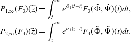 \begin{align*} \begin {aligned} P_{1,\infty }(F_3)(\tilde {z})=\int _{\tilde {z}}^{\infty }e^{\tilde {\alpha }_1(\tilde {z}-t)}F_3(\tilde {\Phi }, \tilde {\Psi })(t)dt,\\ P_{2,\infty }(F_4)(\tilde {z})=\int _{\tilde {z}}^{\infty }e^{\tilde {\alpha }_1(\tilde {z}-t)}F_4(\tilde {\Phi }, \tilde {\Psi })(t)dt.\\ \end {aligned} \end{align*}
Assume that $(\tilde{\Phi }^*(\tilde{z}), \tilde{\Psi }^*(\tilde{z}) )\,:\!=\,(\tilde{\Phi }_1(\tilde{z})+\tilde{W_1}(\tilde{z}), \tilde{\Psi }_1(\tilde{z})+\tilde{W_2}(\tilde{z}))$
, where
$(\tilde{\Phi }^*(\tilde{z}), \tilde{\Psi }^*(\tilde{z}) )\,:\!=\,(\tilde{\Phi }_1(\tilde{z})+\tilde{W_1}(\tilde{z}), \tilde{\Psi }_1(\tilde{z})+\tilde{W_2}(\tilde{z}))$
, where $\tilde{W_1}(\tilde{z})$
and
$\tilde{W_1}(\tilde{z})$
and $\tilde{W_2}(\tilde{z})$
are functions in
$\tilde{W_2}(\tilde{z})$
are functions in $B_0$
that need to be determined. Here,
$B_0$
that need to be determined. Here, $B_0$
is defined as
$B_0$
is defined as
 \begin{align*}B_0=\{u\in C({-}\infty, \infty )\ :\ u(\pm \infty )=0\}.\end{align*}
Therefore, we need to prove the existence of $\tilde{W_1}(\tilde{z})$
and
$\tilde{W_1}(\tilde{z})$
and $\tilde{W_2}(\tilde{z})$
in
$\tilde{W_2}(\tilde{z})$
in $B_0$
such that
$B_0$
such that $(\tilde{\Phi }^*(\tilde{z}), \tilde{\Psi }^*(\tilde{z}) )$
satisfies (3.10) with
$(\tilde{\Phi }^*(\tilde{z}), \tilde{\Psi }^*(\tilde{z}) )$
satisfies (3.10) with $c=\frac{1}{\varepsilon }$
. Plugging
$c=\frac{1}{\varepsilon }$
. Plugging $(\tilde{\Phi }^*(\tilde{z}), \tilde{\Psi }^*(\tilde{z}) )$
into (3.10) and utilising (3.11) lead to
$(\tilde{\Phi }^*(\tilde{z}), \tilde{\Psi }^*(\tilde{z}) )$
into (3.10) and utilising (3.11) lead to
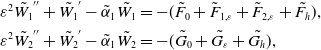 \begin{equation} \begin{aligned} &\varepsilon ^2 \tilde{W_1}^{\prime\prime}+\tilde{W_1}^{\prime}-\tilde{\alpha }_1 \tilde{W_1}=-(\tilde{F_0}+\tilde{F}_{1,\varepsilon }+\tilde{F}_{2,\varepsilon }+\tilde{F_h}),\\ &\varepsilon ^2\tilde{W_2}^{\prime\prime}+\tilde{W_2}^{\prime}-\tilde{\alpha }_1 \tilde{W_2}=-(\tilde{G_0}+\tilde{G_{\varepsilon }}+\tilde{G_h}), \end{aligned} \end{equation}
where
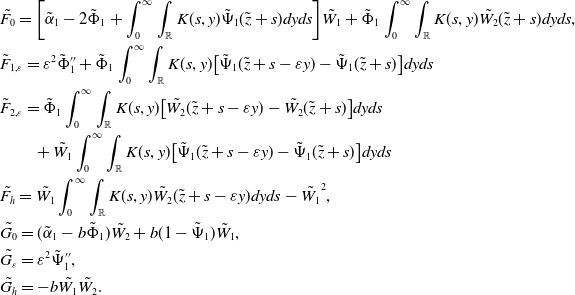 \begin{align*} \begin {aligned} &\tilde {F_0}=\bigg [\tilde {\alpha }_1-2\tilde {\Phi }_1+ \int _{0}^{\infty }\int _{\mathbb {R}} K(s,y)\tilde {\Psi }_1(\tilde {z}+s)dyds\bigg ] \tilde {W_1}+\tilde {\Phi }_1 \int _{0}^{\infty }\int _{\mathbb {R}} K(s,y)\tilde {W_2}(\tilde {z}+s)dyds,\\ &\tilde {F}_{1, \varepsilon }=\varepsilon ^2\tilde {\Phi }_1^{\prime\prime}+\tilde {\Phi }_1 \int _{0}^{\infty }\int _{\mathbb {R}} K(s,y)\big [\tilde {\Psi }_1(\tilde {z}+s-\varepsilon y)-\tilde {\Psi }_1(\tilde {z}+s)\big ]dyds \\ &\tilde {F}_{2,\varepsilon }=\tilde {\Phi }_1 \int _{0}^{\infty }\int _{\mathbb {R}} K(s,y)\big [\tilde {W_2}(\tilde {z}+s-\varepsilon y)-\tilde {W_2}(\tilde {z}+s)\big ]dyds\\ & \quad \quad +\tilde {W_1} \int _{0}^{\infty }\int _{\mathbb {R}} K(s,y)\big [\tilde {\Psi }_1(\tilde {z}+s-\varepsilon y)-\tilde {\Psi }_1(\tilde {z}+s)\big ]dyds\\ &\tilde {F_h}=\tilde {W_1} \int _{0}^{\infty }\int _{\mathbb {R}} K(s,y)\tilde {W_2}(\tilde {z}+s-\varepsilon y)dyds-\tilde {W_1}^2,\\ &\tilde {G_0}=(\tilde {\alpha }_1-b\tilde {\Phi }_1)\tilde {W_2}+b(1-\tilde {\Psi }_1)\tilde {W_1},\\ &\tilde {G_\varepsilon }=\varepsilon ^2\tilde {\Psi }_1^{\prime\prime},\\ &\tilde {G_h}=-b\tilde {W_1}\tilde {W_2}. \end {aligned} \end{align*}
Therefore, we have
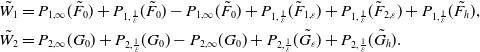 \begin{equation} \begin{aligned} &\tilde{W_1}=P_{1,\infty }(\tilde{F_0})+ P_{1,\frac{1}{\varepsilon }}(\tilde{F_0})-P_{1,\infty }(\tilde{F_0})+ P_{1,\frac{1}{\varepsilon }}(\tilde{F}_{1,\varepsilon })+P_{1,\frac{1}{\varepsilon }}(\tilde{F}_{2,\varepsilon })+P_{1,\frac{1}{\varepsilon }}(\tilde{F_h}),\\ &\tilde{W_2}=P_{2,\infty }(G_0)+P_{2,\frac{1}{\varepsilon }}(G_0)-P_{2,\infty }(G_0)+P_{2,\frac{1}{\varepsilon }}(\tilde{G_\varepsilon })+P_{2,\frac{1}{\varepsilon }}(\tilde{G_h}). \end{aligned} \end{equation}
Define
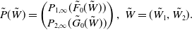 \begin{align*} \tilde {P}(\tilde {W})= \begin {pmatrix} P_{1,\infty }(\tilde {F_0}(\tilde {W}))\\ P_{2,\infty }(\tilde {G_0}(\tilde {W})) \end {pmatrix}, \ \tilde {W}=(\tilde {W_1}, \tilde {W_2}). \end{align*}
By a simple estimate, we have
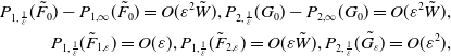 \begin{align*}P_{1,\frac {1}{\varepsilon }}(\tilde {F_0})-P_{1,\infty }(\tilde {F_0})= O(\varepsilon ^2\tilde {W}), P_{2,\frac {1}{\varepsilon }}(G_0)-P_{2,\infty }(G_0)=O(\varepsilon ^2\tilde {W}),\\ P_{1,\frac {1}{\varepsilon }}(\tilde {F}_{1, \varepsilon })=O(\varepsilon ), P_{1,\frac {1}{\varepsilon }}(\tilde {F}_{2, \varepsilon })=O(\varepsilon \tilde {W}), P_{2,\frac {1}{\varepsilon }}(\tilde {G_\varepsilon })=O(\varepsilon ^2),\end{align*}
and $ P_{1,\frac{1}{\varepsilon }}(\tilde{F}_{1, \varepsilon })=o(\tilde{z}^{-3})$
as
$ P_{1,\frac{1}{\varepsilon }}(\tilde{F}_{1, \varepsilon })=o(\tilde{z}^{-3})$
as $\tilde{z}\rightarrow \infty$
. The linear operator
$\tilde{z}\rightarrow \infty$
. The linear operator $\tilde{P}$
is both compact and strongly positive. It possesses a simple principal eigenvalue
$\tilde{P}$
is both compact and strongly positive. It possesses a simple principal eigenvalue $\lambda =1$
with the corresponding positive eigenfunction
$\lambda =1$
with the corresponding positive eigenfunction $({-}\tilde{\Phi }_1^{\prime},-\tilde{\Psi }_1^{\prime})$
. To eliminate this eigenfunction from
$({-}\tilde{\Phi }_1^{\prime},-\tilde{\Psi }_1^{\prime})$
. To eliminate this eigenfunction from $B_0$
, we introduce the weighted functional space as follows
$B_0$
, we introduce the weighted functional space as follows
 \begin{align*} \mathcal {H}=\{h(\tilde {z})\in B_0\ :\ h\tilde {z}^3=o(1) \quad \rm {as} \quad \tilde {z} \rightarrow \infty \}. \end{align*}
Since the eigenfunction $({-}\tilde{\Phi }_1^{\prime},-\tilde{\Psi }_1^{\prime})$
does not belong to the space
$({-}\tilde{\Phi }_1^{\prime},-\tilde{\Psi }_1^{\prime})$
does not belong to the space $\mathcal{H}\times B_0$
, it implies that
$\mathcal{H}\times B_0$
, it implies that $\tilde{P}$
does not possess the eigenvalue
$\tilde{P}$
does not possess the eigenvalue $\lambda =1$
in the functional space
$\lambda =1$
in the functional space $\mathcal{H}\times B_0$
. Consequently,
$\mathcal{H}\times B_0$
. Consequently, $I-\tilde{P}$
has a bounded inverse in
$I-\tilde{P}$
has a bounded inverse in $\mathcal{H}\times B_0$
, where
$\mathcal{H}\times B_0$
, where $I$
is the identity operator. By applying the abstract implicit function theorem in
$I$
is the identity operator. By applying the abstract implicit function theorem in $\mathcal{H}\times B_0$
, we conclude that there exists
$\mathcal{H}\times B_0$
, we conclude that there exists $\varepsilon _0$
such that a solution
$\varepsilon _0$
such that a solution $(\tilde{W_1},\tilde{W_2})$
of the system (3.20) exists for any
$(\tilde{W_1},\tilde{W_2})$
of the system (3.20) exists for any $\varepsilon \in [0, \varepsilon _0)$
. Consequently, there exists a solution
$\varepsilon \in [0, \varepsilon _0)$
. Consequently, there exists a solution $(\tilde{\Phi }^*(\tilde{z}), \tilde{\Psi }^*(\tilde{z}) )$
of (3.10) for all
$(\tilde{\Phi }^*(\tilde{z}), \tilde{\Psi }^*(\tilde{z}) )$
of (3.10) for all $c\ge \tilde{M}\gt \frac{1}{\varepsilon _0}$
, with decay behaviour (3.16).
$c\ge \tilde{M}\gt \frac{1}{\varepsilon _0}$
, with decay behaviour (3.16).
Step 3. By continuation and the abstract implicit function theorem, we further prove the existence of monostable monotone travelling waves of system (3.10) for $c= \tilde{M}-\delta$
, with
$c= \tilde{M}-\delta$
, with $\delta$
is a sufficiently small and to-be-determined value. Let
$\delta$
is a sufficiently small and to-be-determined value. Let $(\tilde{\Phi }_2(\tilde{z}), \tilde{\Psi }_2(\tilde{z}))$
be the solution of (3.10) for
$(\tilde{\Phi }_2(\tilde{z}), \tilde{\Psi }_2(\tilde{z}))$
be the solution of (3.10) for $c=c_2= \tilde{M}$
. Thus, we have
$c=c_2= \tilde{M}$
. Thus, we have
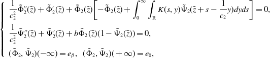 \begin{equation} \left \{ \begin{array}{cc} \begin{aligned} &\frac{1}{c_2^2}\tilde{\Phi }_2^{\prime\prime}(\tilde{z})+\tilde{\Phi }_2^{\prime}(\tilde{z})+\tilde{\Phi }_2(\tilde{z})\bigg [{-}\tilde{\Phi }_2(\tilde{z})+\int _{0}^{\infty }\int _{\mathbb{R}} K(s,y)\tilde{\Psi }_2(\tilde{z}+s-\frac{1}{c_2}y)dyds\bigg ] =0, \\[3pt] &\frac{1}{c_2^2}\tilde{\Psi }_2^{\prime\prime}(\tilde{z})+\tilde{\Psi }_2^{\prime}(\tilde{z})+b\tilde{\Phi }_2(\tilde{z})(1-\tilde{\Psi }_2(\tilde{z}))=0, \\[3pt] &(\tilde{\Phi }_2, \tilde{\Psi }_2)({-}\infty )=e_\beta, \ \ (\tilde{\Phi }_2, \tilde{\Psi }_2)(+\infty )=e_0, \end{aligned} \end{array}\right . \end{equation}
Assuming $c=c_\delta =c_2-\delta$
. To find the solution of (3.17), say
$c=c_\delta =c_2-\delta$
. To find the solution of (3.17), say $(\bar{\Phi }_\delta (\tilde{z}), \bar{\Psi }_\delta (\tilde{z}))$
at
$(\bar{\Phi }_\delta (\tilde{z}), \bar{\Psi }_\delta (\tilde{z}))$
at $c=c_{\delta }$
, we let
$c=c_{\delta }$
, we let $\bar{\Phi }_\delta (\tilde{z})=\tilde{\Phi }_2(\tilde{z})+\bar{W}_1(\tilde{z})$
and
$\bar{\Phi }_\delta (\tilde{z})=\tilde{\Phi }_2(\tilde{z})+\bar{W}_1(\tilde{z})$
and $\bar{\Psi }_\delta (\tilde{z})=\tilde{\Psi }_2(\tilde{z})+\bar{W}_2(\tilde{z})$
, where
$\bar{\Psi }_\delta (\tilde{z})=\tilde{\Psi }_2(\tilde{z})+\bar{W}_2(\tilde{z})$
, where $\bar{W}_1(\tilde{z})$
and
$\bar{W}_1(\tilde{z})$
and $\bar{W}_2(\tilde{z})$
are functions in
$\bar{W}_2(\tilde{z})$
are functions in $B_0$
that need to be determined. Thus, we aim to prove the existence of
$B_0$
that need to be determined. Thus, we aim to prove the existence of $\bar{W}_1(\tilde{z})$
and
$\bar{W}_1(\tilde{z})$
and $\bar{W}_2(\tilde{z})$
in
$\bar{W}_2(\tilde{z})$
in $B_0$
such that
$B_0$
such that $(\bar{\Phi }_\delta (\tilde{z}), \bar{\Psi }_\delta (\tilde{z}))$
satisfies (3.10) or (3.17) with speed
$(\bar{\Phi }_\delta (\tilde{z}), \bar{\Psi }_\delta (\tilde{z}))$
satisfies (3.10) or (3.17) with speed $c_\delta$
. Substituting
$c_\delta$
. Substituting $(\bar{\Phi }_\delta (\tilde{z}), \bar{\Psi }_\delta (\tilde{z}))$
into (3.10) and using (3.22) give
$(\bar{\Phi }_\delta (\tilde{z}), \bar{\Psi }_\delta (\tilde{z}))$
into (3.10) and using (3.22) give
 \begin{equation} \begin{aligned} &\bar{W}_1=P_{1,c_2}(\bar{F}_0)+P_{1,c_\delta }(\bar{F}_0)-P_{1,c_2}(\bar{F}_0) + P_{1,c_\delta }(\bar{F}_{1,\delta })+P_{1,c_\delta }(\bar{F}_{2,\delta })+P_{1,c_\delta }(\bar{F}_h),\\ &\bar{W}_2=P_{2,c_2}(\bar{G}_0)+ P_{2,c_\delta }(\bar{G}_0)-P_{2,c_2}(\bar{G}_0)+P_{2,c_\delta }(\bar{G}_\delta )+P_{2,c_\delta }(\bar{G}_h), \end{aligned} \end{equation}
where
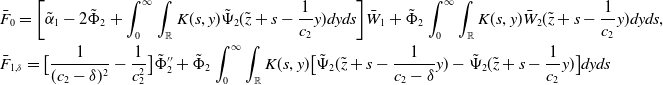 \begin{align*} \begin {aligned} &\bar {F}_0=\bigg [\tilde {\alpha }_1-2\tilde {\Phi }_2+\int _{0}^{\infty }\int _{\mathbb {R}} K(s,y)\tilde {\Psi }_2(\tilde {z}+s-\frac {1}{c_2}y)dyds\bigg ] \bar {W}_1+\tilde {\Phi }_2\int _{0}^{\infty }\int _{\mathbb {R}} K(s,y)\bar {W}_2(\tilde {z}+s-\frac {1}{c_2}y)dyds,\\ &\bar {F}_{1, \delta }=\big [\frac {1}{(c_2-\delta )^2}-\frac {1}{c_2^2}\big ]\tilde {\Phi }_2^{\prime\prime}+\tilde {\Phi }_2 \int _{0}^{\infty }\int _{\mathbb {R}} K(s,y)\big [\tilde {\Psi }_2(\tilde {z}+s-\frac {1}{c_2-\delta } y)-\tilde {\Psi }_2(\tilde {z}+s-\frac {1}{c_2}y)\big ]dyds \end {aligned} \end{align*}
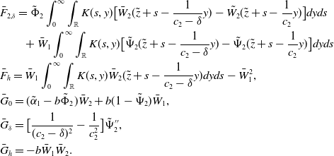 \begin{align*} \begin {aligned} &\bar {F}_{2,\delta }=\tilde {\Phi }_2 \int _{0}^{\infty }\int _{\mathbb {R}} K(s,y)\big [\bar {W}_2(\tilde {z}+s-\frac {1}{c_2-\delta }y)-\tilde {W_2}(\tilde {z}+s-\frac {1}{c_2}y)\big ]dyds\\ & \quad \quad +\bar {W}_1 \int _{0}^{\infty }\int _{\mathbb {R}} K(s,y)\big [\tilde {\Psi }_2(\tilde {z}+s-\frac {1}{c_2-\delta }y)-\tilde {\Psi }_2(\tilde {z}+s-\frac {1}{c_2}y)\big ]dyds\\ &\bar {F}_h=\bar {W}_1 \int _{0}^{\infty }\int _{\mathbb {R}} K(s,y)\bar {W}_2(\tilde {z}+s-\frac {1}{c_2-\delta }y)dyds-\bar {W}_1^2,\\ &\bar {G}_0=(\tilde {\alpha }_1-b\tilde {\Phi }_2)\bar {W}_2+b(1-\tilde {\Psi }_2)\bar {W}_1,\\ &\bar {G}_\delta =\big [\frac {1}{(c_2-\delta )^2}-\frac {1}{c_2^2}\big ]\tilde {\Psi }_2^{\prime\prime},\\ &\bar {G}_h=-b\bar {W}_1\bar {W}_2. \end {aligned} \end{align*}
Define
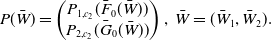 \begin{align*} P(\bar {W})= \begin {pmatrix} P_{1,c_2}(\bar {F}_0(\bar {W}))\\ P_{2,c_2}(\bar {G}_0(\bar {W})) \end {pmatrix}, \ \bar {W}=(\bar {W}_1, \bar {W}_2). \end{align*}
Clearly, we have
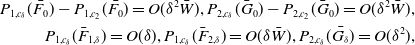 \begin{align*}P_{1,c_\delta }(\bar {F_0})-P_{1,c_2}(\bar {F_0})= O(\delta ^2\bar {W}), P_{2,c_\delta }(\bar {G}_0)-P_{2,c_2}(\bar {G}_0)=O(\delta ^2\bar {W}),\\P_{1,c_\delta }(\bar {F}_{1,\delta })=O(\delta ), P_{1,c_\delta }(\bar {F}_{2,\delta })=O(\delta \bar {W}), P_{2,c_\delta }(\bar {G_\delta })=O(\delta ^2),\end{align*}
and $ P_{1,c_\delta }(\bar{F}_{1,\delta })=o(\tilde{z}^{-3})$
as
$ P_{1,c_\delta }(\bar{F}_{1,\delta })=o(\tilde{z}^{-3})$
as $\tilde{z}\rightarrow \infty$
. The linear operator
$\tilde{z}\rightarrow \infty$
. The linear operator $P$
is both compact and strongly positive. It possesses a simple principal eigenvalue
$P$
is both compact and strongly positive. It possesses a simple principal eigenvalue $\lambda =1$
with the corresponding positive eigenfunction
$\lambda =1$
with the corresponding positive eigenfunction $({-}\tilde{\Phi }_2^{\prime},-\tilde{\Psi }_2^{\prime})$
. By a similar argument as in Step 2, the eigenfunction
$({-}\tilde{\Phi }_2^{\prime},-\tilde{\Psi }_2^{\prime})$
. By a similar argument as in Step 2, the eigenfunction $({-}\tilde{\Phi }_2^{\prime},-\tilde{\Psi }_2^{\prime})$
does not belong to the space
$({-}\tilde{\Phi }_2^{\prime},-\tilde{\Psi }_2^{\prime})$
does not belong to the space $\mathcal{H}\times B_0$
. It follows from the abstract implicit function theorem in
$\mathcal{H}\times B_0$
. It follows from the abstract implicit function theorem in $\mathcal{H}\times B_0$
that there exists
$\mathcal{H}\times B_0$
that there exists $\delta _0$
such that a solution
$\delta _0$
such that a solution $(\bar{W}_1,\bar{W}_2)$
of the system (3.23) exists for any
$(\bar{W}_1,\bar{W}_2)$
of the system (3.23) exists for any $\delta \in [0, \delta _0)$
. Consequently, there exists a solution
$\delta \in [0, \delta _0)$
. Consequently, there exists a solution $(\bar{\Phi }_\delta (\tilde{z}), \bar{\Psi }_\delta (\tilde{z}))$
of (3.10) with
$(\bar{\Phi }_\delta (\tilde{z}), \bar{\Psi }_\delta (\tilde{z}))$
of (3.10) with $c=c_\delta$
.
$c=c_\delta$
.
Step 4. Note that $\mu _1=0$
and
$\mu _1=0$
and $\mu _2=c$
from (3.2) for
$\mu _2=c$
from (3.2) for $r=1$
. When
$r=1$
. When $c\gt c_{\min }^{\bar{r}}$
, Theorem3.2 implies that if travelling wave solutions of (1.5)-(1.6) with
$c\gt c_{\min }^{\bar{r}}$
, Theorem3.2 implies that if travelling wave solutions of (1.5)-(1.6) with $r=1$
exist, they do not decay exponentially to
$r=1$
exist, they do not decay exponentially to $0$
as
$0$
as $z\rightarrow \infty$
. This indicates that travelling wave solutions of (3.10), if they exist, exhibit algebraic decay behaviour (3.16) for all
$z\rightarrow \infty$
. This indicates that travelling wave solutions of (3.10), if they exist, exhibit algebraic decay behaviour (3.16) for all $c\gt c_{\min }^{\bar{r}}$
. By repeating the continuation process from Step 3, we establish the existence of monostable monotone travelling waves of system (3.10) for all
$c\gt c_{\min }^{\bar{r}}$
. By repeating the continuation process from Step 3, we establish the existence of monostable monotone travelling waves of system (3.10) for all $c\in (c_{\min }^{\bar{r}}, \tilde{M})$
. Therefore, we prove that when
$c\in (c_{\min }^{\bar{r}}, \tilde{M})$
. Therefore, we prove that when $r=1$
, there is a finite
$r=1$
, there is a finite $c_{\min }^{\bar{r}}\gt 0$
such that monotone and positive travelling wave solutions of (1.5)-(1.6) exist if and only if
$c_{\min }^{\bar{r}}\gt 0$
such that monotone and positive travelling wave solutions of (1.5)-(1.6) exist if and only if $c\ge c_{\min }^{\bar{r}}$
. When
$c\ge c_{\min }^{\bar{r}}$
. When $c\gt c_{\min }^{\bar{r}}$
, the travelling wave solution
$c\gt c_{\min }^{\bar{r}}$
, the travelling wave solution $(\Phi, \Psi )(z)$
of (1.5)-(1.6) has the following algebraic decay behaviour
$(\Phi, \Psi )(z)$
of (1.5)-(1.6) has the following algebraic decay behaviour
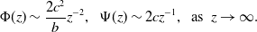 \begin{align*} \Phi (z) \sim \frac {2c^2}{b} z^{-2}, \ \ \Psi (z) \sim 2c z^{-1}, \ \ \text {as} \ \ z\rightarrow \infty . \end{align*}
3.2. Speed selection
In this subsection, we shall derive some conditions for speed selection. The subsequent theorem provides a necessary and sufficient condition for nonlinear selection, which is a development of the abstract results of speed selection in [Reference Ma and Ou23] to the system (1.1).
Theorem 3.4.
Assume that H2 and (K1) hold. The minimal wave speed $c_{\min }$
of (1.5)-(1.6) is nonlinearly selected if and only if there exists a wavefront
$c_{\min }$
of (1.5)-(1.6) is nonlinearly selected if and only if there exists a wavefront $(c_2,\Phi, \Psi )$
,
$(c_2,\Phi, \Psi )$
, $c_2\gt c_0$
such that
$c_2\gt c_0$
such that
 \begin{align*}\Phi (z)\sim A_2e^{-\mu _2(c_2) z},\ \text {as} \ z\rightarrow \infty, \ z=\nu {\cdot}x-c_2t,\ ||\nu ||=1,\end{align*}
with $A_2\gt 0$
. Furthermore,
$A_2\gt 0$
. Furthermore, $c_2=c_{\min }$
.
$c_2=c_{\min }$
.
Proof. To establish the necessity, we assume that the minimal wave speed is nonlinearly selected, denoted as $c_{\min } \gt c_0$
. Our goal is to demonstrate that the travelling wave
$c_{\min } \gt c_0$
. Our goal is to demonstrate that the travelling wave $(\Phi _2(z), \Psi _2(z))$
of system (1.5)-(1.6), with a speed
$(\Phi _2(z), \Psi _2(z))$
of system (1.5)-(1.6), with a speed $c = c_2 = c_{\min }$
, exhibits the following behaviour
$c = c_2 = c_{\min }$
, exhibits the following behaviour
 \begin{align*} \Phi _2(z)\sim A_2e^{-\mu _2(c_2) z},\ \text {as} \ z\rightarrow \infty, \ z=\nu {\cdot}x-c_2t,\ ||\nu ||=1, \end{align*}
with $A_2\gt 0$
. To the contrary, we assume that
$A_2\gt 0$
. To the contrary, we assume that
 \begin{equation} \Phi _2(z)\sim A_2e^{-\mu _1(c_2) z},\ \text{as} \ z\rightarrow \infty, \ \ \text{for} \ r\in (0,1) \end{equation}
and
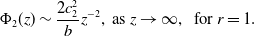 \begin{equation} \Phi _2(z)\sim \frac{2c_2^2}{b}z^{-2},\ \text{as} \ z\rightarrow \infty, \ \ \text{for} \ r=1. \end{equation}
By a similar argument in Step 3 of Theorem3.3, we can prove that there is a monotone travelling wave solution of (1.5)-(1.6) when $c=c_\delta =c_2-\delta$
, where
$c=c_\delta =c_2-\delta$
, where $\delta$
is a sufficiently small and to-be-determined value. It implies that
$\delta$
is a sufficiently small and to-be-determined value. It implies that $c_2$
is not the minimum wave speed. This contradiction establishes the necessity. Clearly, for
$c_2$
is not the minimum wave speed. This contradiction establishes the necessity. Clearly, for $r=1$
, Step 3 of Theorem3.3 shows the existence of monotone travelling wave solution of (1.5)-(1.6) when
$r=1$
, Step 3 of Theorem3.3 shows the existence of monotone travelling wave solution of (1.5)-(1.6) when $c=c_2-\delta$
with a small
$c=c_2-\delta$
with a small $\delta$
. Thus, we only focus on
$\delta$
. Thus, we only focus on $r\in (0,1)$
. Let
$r\in (0,1)$
. Let $\alpha$
be large enough so that
$\alpha$
be large enough so that
 \begin{align*} F(\Phi, \Psi )\,:\!=\,\alpha \Phi +\Phi (1-r-\Phi +r(K\star _c\Psi )) \end{align*}
and
 \begin{align*} G(\Phi, \Psi )\,:\!=\,\alpha \Psi +b\Phi (1-\Psi ) \end{align*}
are non-decreasing functions of $\Phi$
and
$\Phi$
and $\Psi$
. Then we can express system (1.5) as
$\Psi$
. Then we can express system (1.5) as
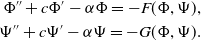 \begin{equation} \begin{aligned} \Phi ^{\prime\prime}+c\Phi ^{\prime}-\alpha \Phi =-F(\Phi, \Psi ),\\ \Psi ^{\prime\prime}+c\Psi ^{\prime}-\alpha \Psi =-G(\Phi, \Psi ).\\ \end{aligned} \end{equation}
Define $\beta _1$
and
$\beta _1$
and $\beta _2$
as
$\beta _2$
as
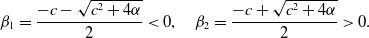 \begin{equation} \beta _1=\frac{-c-\sqrt{c^2+4\alpha }}{2}\lt 0, \quad \beta _2=\frac{-c+\sqrt{c^2+4\alpha }}{2}\gt 0. \end{equation}
In view of the variation of parameters, the integral form of (3.26) is given by
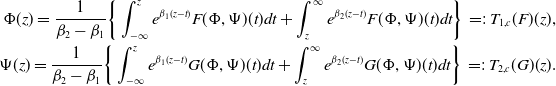 \begin{equation} \begin{aligned} \Phi (z)=\frac{1}{\beta _2-\beta _1}\bigg \{\int _{-\infty }^{z}e^{\beta _1(z-t)}F(\Phi, \Psi )(t)dt+\int _{z}^{\infty }e^{\beta _2(z-t)}F(\Phi, \Psi )(t)dt\bigg \} \,=\!:\,T_{1,c}(F)(z),\\ \Psi (z)=\frac{1}{\beta _2-\beta _1}\bigg \{\int _{-\infty }^{z}e^{\beta _1(z-t)}G(\Phi, \Psi )(t)dt+\int _{z}^{\infty }e^{\beta _2(z-t)}G(\Phi, \Psi )(t)dt\bigg \} \,=\!:\,T_{2,c}(G)(z).\\ \end{aligned} \end{equation}
Note that $(\Phi _2(z), \Psi _2(z))$
satisfies
$(\Phi _2(z), \Psi _2(z))$
satisfies
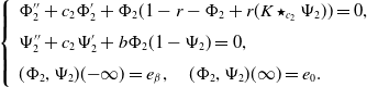 \begin{equation} \left \{ \begin{array}{cc} \begin{aligned} &\Phi _2^{\prime\prime}+c_2\Phi _2^{\prime}+\Phi _2(1-r-\Phi _2+r(K\star _{c_2}\Psi _2))=0,\\[3pt] &\Psi _2^{\prime\prime}+c_2\Psi _2^{\prime}+b\Phi _2(1-\Psi _2)=0,\\[3pt] &(\Phi _2, \Psi _2)({-}\infty )=e_\beta, \quad (\Phi _2, \Psi _2)(\infty )=e_0. \end{aligned} \end{array} \right . \end{equation}
Define $\bar{\Phi }(z)=\Phi _2(z) \omega (z)$
, where
$\bar{\Phi }(z)=\Phi _2(z) \omega (z)$
, where
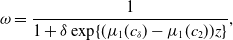 \begin{align*} \omega = \frac {1}{1+\delta \exp \{(\mu _1(c_\delta )-\mu _1(c_2))z\}}, \end{align*}
Using asymptotic analysis, we can deduce that
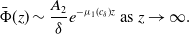 \begin{align*} \bar {\Phi }(z)\sim \frac {A_2}{\delta }e^{-\mu _1(c_\delta )z} \ \text {as} \ z\rightarrow \infty . \end{align*}
To find the solution of (3.26), say $(\Phi _\delta (z), \Psi _\delta (z))$
, at
$(\Phi _\delta (z), \Psi _\delta (z))$
, at $c=c_{\delta }$
, we introduce
$c=c_{\delta }$
, we introduce $\Phi _\delta (z)$
as
$\Phi _\delta (z)$
as $\Phi _\delta (z)=\bar{\Phi }(z)+W_1(z)$
and
$\Phi _\delta (z)=\bar{\Phi }(z)+W_1(z)$
and $\Psi _\delta (z)$
as
$\Psi _\delta (z)$
as $\Psi _\delta (z)=\Psi _2(z)+W_2(z)$
, where
$\Psi _\delta (z)=\Psi _2(z)+W_2(z)$
, where $W_1(z)$
and
$W_1(z)$
and $W_2(z)$
are functions in
$W_2(z)$
are functions in $B_0$
that need to be determined. Here,
$B_0$
that need to be determined. Here, $B_0$
is defined inTheorem3.3. By substituting
$B_0$
is defined inTheorem3.3. By substituting $(\Phi _\delta (z), \Psi _\delta (z))$
into (1.5) and utilising (3.29), we observe that
$(\Phi _\delta (z), \Psi _\delta (z))$
into (1.5) and utilising (3.29), we observe that $W_1$
and
$W_1$
and $W_2$
fulfill the following equations
$W_2$
fulfill the following equations
 \begin{equation} \begin{aligned} &W_1=T_{1,c_2}(F_0)+T_{1,c_\delta }(F_0)-T_{1,c_2}(F_0)+ T_{1,c_\delta }(F_{1,\delta })+ T_{1,c_\delta }(F_{2,\delta })+T_{1,c_\delta }(F_h),\\ &W_2=T_{2,c_2}(G_0)+T_{2,c_\delta }(G_0)-T_{2,c_2}(G_0)+T_{2,c_\delta }(G_{1,\delta })+T_{2,c_\delta }(G_{2,\delta })+T_{2,c_\delta }(G_h) \end{aligned} \end{equation}
where
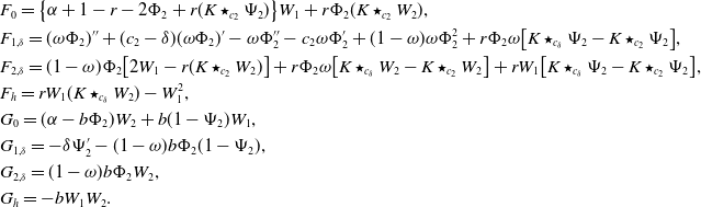 \begin{align*} \begin {aligned} &F_0=\big \{\alpha +1-r-2\Phi _2+r(K\star _{c_2}\Psi _2)\big \} W_1+r\Phi _2(K\star _{c_2} W_2),\\ &F_{1,\delta }=(\omega \Phi _2)^{\prime\prime}+(c_2-\delta )(\omega \Phi _2)^{\prime}-\omega \Phi _2^{\prime\prime}-c_2\omega \Phi _2^{\prime} +(1-\omega )\omega \Phi _2^2+r\Phi _2\omega \big [K\star _{c_\delta }\Psi _2-K\star _{c_2}\Psi _2 \big ],\\ &F_{2,\delta }=(1-\omega )\Phi _2\big [ 2W_1-r(K\star _{c_2} W_2)\big ]+r\Phi _2\omega \big [K\star _{c_\delta }W_2-K\star _{c_2}W_2\big ]+rW_1\big [K\star _{c_\delta }\Psi _2-K\star _{c_2}\Psi _2 \big ], \\ &F_h=rW_1 (K\star _{c_\delta } W_2)-W_1^2,\\ &G_0=(\alpha -b\Phi _2)W_2+b(1-\Psi _2)W_1,\\ &G_{1,\delta }=-\delta \Psi _2^{\prime}-(1-\omega )b\Phi _2(1-\Psi _2),\\ &G_{2,\delta }=(1-\omega )b\Phi _2W_2,\\ &G_h=-bW_1W_2. \end {aligned} \end{align*}
Define
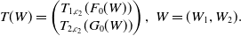 \begin{align*} T(W)= \begin {pmatrix} T_{1,c_2}(F_0(W))\\ T_{2,c_2}(G_0(W)) \end {pmatrix}, \ W=(W_1, W_2). \end{align*}
It is worth noting that $\omega ^{\prime}=-(\mu _1(c_\delta )-\mu _1(c_2))\omega (1-\omega )$
and
$\omega ^{\prime}=-(\mu _1(c_\delta )-\mu _1(c_2))\omega (1-\omega )$
and $\omega ^{\prime\prime}=(\mu _1(c_\delta )-\mu _1(c_2))^2\omega (1-\omega )(1-2\omega )$
. Clearly, we have
$\omega ^{\prime\prime}=(\mu _1(c_\delta )-\mu _1(c_2))^2\omega (1-\omega )(1-2\omega )$
. Clearly, we have
 \begin{align*}T_{1,c_\delta }(F_0)-T_{1,c_2}(F_0) & = O(\delta W), T_{2,c_\delta }(G_0)-T_{2,c_2}(G_0)=O(\delta W),\\T_{1,c_\delta }(F_{1,\delta })=O(\delta ), T_{1,c_\delta }(F_{2,\delta }) & = O(\delta W), T_{2,c_\delta }(G_{1,\delta })=O(\delta ), T_{2,c_\delta }(G_{2,\delta })=O(\delta W), \end{align*}
and $T_{1,c_\delta }(F_{1,\delta })=o(e^{-\mu _1(c_\delta ) z})$
as
$T_{1,c_\delta }(F_{1,\delta })=o(e^{-\mu _1(c_\delta ) z})$
as $z\rightarrow \infty$
. The linear operator
$z\rightarrow \infty$
. The linear operator $T$
is both compact and strongly positive. It possesses a simple principal eigenvalue
$T$
is both compact and strongly positive. It possesses a simple principal eigenvalue $\lambda =1$
with the corresponding positive eigenfunction
$\lambda =1$
with the corresponding positive eigenfunction $({-}\Phi _2^{\prime},-\Psi _2^{\prime})$
. Here, we introduce another weighted functional space
$({-}\Phi _2^{\prime},-\Psi _2^{\prime})$
. Here, we introduce another weighted functional space
 \begin{align*} \mathcal {H}_1=\{h(\xi )\in B_0\ :\ he^{\mu _1(c_\delta )\xi }=o(1) \quad \rm {as} \quad \xi \rightarrow \infty \} \end{align*}
to remove eigenfunction $({-}\Phi _2^{\prime},-\Psi _2^{\prime})$
from
$({-}\Phi _2^{\prime},-\Psi _2^{\prime})$
from $B_0$
. Similar to Step 3 of Theorem3.3, by applying the abstract implicit function theorem in
$B_0$
. Similar to Step 3 of Theorem3.3, by applying the abstract implicit function theorem in $\mathcal{H}_1\times B_0$
, we conclude that there exists
$\mathcal{H}_1\times B_0$
, we conclude that there exists $\delta _1$
such that a solution
$\delta _1$
such that a solution $(W_1,W_2)$
of the system (3.30) exists for any
$(W_1,W_2)$
of the system (3.30) exists for any $\delta \in [0, \delta _1)$
when
$\delta \in [0, \delta _1)$
when $r\in (0,1)$
. Consequently, there exists a solution
$r\in (0,1)$
. Consequently, there exists a solution $(\Phi _\delta (z), \Psi _\delta (z))$
of (1.5)-(1.6) with
$(\Phi _\delta (z), \Psi _\delta (z))$
of (1.5)-(1.6) with $c=c_\delta$
when
$c=c_\delta$
when $r\in (0,1)$
.
$r\in (0,1)$
.
The sufficiency result follows from Theorem3.2.
The result above relies on an assumption about the wave solution, which is generally unknown. To overcome this difficulty, we will provide a theorem that offers a convenient approach for the nonlinear or linear selection of the minimal wave speed in system (1.5)-(1.6).
Theorem 3.5.
(Linear, nonlinear selection and estimate of $c_{\min }$
) Assume that H2 and (K1) hold.
$c_{\min }$
) Assume that H2 and (K1) hold.
(i) For $c_1\gt c_0$
, if there exists a nonnegative and monotonic lower solution
$c_1\gt c_0$
, if there exists a nonnegative and monotonic lower solution $(\underline{\Phi },\underline{\Psi })(z)$
of system (1.5)-(1.6) such that
$(\underline{\Phi },\underline{\Psi })(z)$
of system (1.5)-(1.6) such that $\underline{\Phi }(z)\sim \underline{A} e^{-\mu _2 z}$
as
$\underline{\Phi }(z)\sim \underline{A} e^{-\mu _2 z}$
as $z\rightarrow \infty$
with
$z\rightarrow \infty$
with $\underline{A}\gt 0$
, and
$\underline{A}\gt 0$
, and $\limsup _{z\rightarrow -\infty }\underline{\Phi }(z)\lt 1$
, then no travelling wave solution exists for
$\limsup _{z\rightarrow -\infty }\underline{\Phi }(z)\lt 1$
, then no travelling wave solution exists for $c\in [c_0, c_1)$
and there exists
$c\in [c_0, c_1)$
and there exists $c_{\min }\gt c_1$
.
$c_{\min }\gt c_1$
.
(ii) For $r\in (0,1)$
and
$r\in (0,1)$
and $c=c_0+\varepsilon$
where
$c=c_0+\varepsilon$
where $\varepsilon$
is any small positive number, if there exists a nonnegative and monotonic upper solution
$\varepsilon$
is any small positive number, if there exists a nonnegative and monotonic upper solution $(\overline{\Phi },\overline{\Psi })(z)$
of system (1.5)-(1.6) such that
$(\overline{\Phi },\overline{\Psi })(z)$
of system (1.5)-(1.6) such that $\overline{\Phi }(z)\sim \overline{A} e^{-\mu _1(c) z}$
as
$\overline{\Phi }(z)\sim \overline{A} e^{-\mu _1(c) z}$
as $z\rightarrow \infty$
with
$z\rightarrow \infty$
with $\overline{A}\gt 0$
, and
$\overline{A}\gt 0$
, and $\limsup _{z\rightarrow -\infty }\overline{\Phi }(z)\ge 1$
, then we have
$\limsup _{z\rightarrow -\infty }\overline{\Phi }(z)\ge 1$
, then we have $c_{\min }=c_0$
.
$c_{\min }=c_0$
.
Proof. (i) On the contrary, we assume that for $c\in (c_0, c_1)$
, there exists a monotone travelling wave solution
$c\in (c_0, c_1)$
, there exists a monotone travelling wave solution $(\Phi, \Psi )(\nu\ {\cdot}\ x-ct)$
of the system (1.2) with the initial conditions
$(\Phi, \Psi )(\nu\ {\cdot}\ x-ct)$
of the system (1.2) with the initial conditions
 \begin{align*} \phi (0,x)=\Phi (\nu\ {\cdot}\ x),\quad \psi (0,x)=\Psi (\nu\ {\cdot}\ x). \end{align*}
Note that $\underline{\Phi }(\nu\ {\cdot}\ x)\le \Phi (\nu\ {\cdot}\ x)$
for
$\underline{\Phi }(\nu\ {\cdot}\ x)\le \Phi (\nu\ {\cdot}\ x)$
for $x\in \mathbb{R}^n$
by shifting if necessary. According to
$x\in \mathbb{R}^n$
by shifting if necessary. According to $\Psi$
-equation of (1.5), we have
$\Psi$
-equation of (1.5), we have $(\underline{\Phi },\underline{\Psi })(\nu\ {\cdot}\ x)\le (\Phi, \Psi )(\nu\ {\cdot}\ x)$
for
$(\underline{\Phi },\underline{\Psi })(\nu\ {\cdot}\ x)\le (\Phi, \Psi )(\nu\ {\cdot}\ x)$
for $x\in \mathbb{R}^n$
. By the comparison theorem, we obtain
$x\in \mathbb{R}^n$
. By the comparison theorem, we obtain
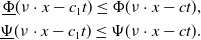 \begin{align*} \underline {\Phi }(\nu\ {\cdot}\ x-c_1t)\le \Phi (\nu\ {\cdot}\ x-ct),\\\underline {\Psi }(\nu\ {\cdot}\ x-c_1t)\le \Psi (\nu\ {\cdot}\ x-ct). \end{align*}
Fix $z^*=\nu {\cdot}x-c_1t$
such that
$z^*=\nu {\cdot}x-c_1t$
such that $\underline{\Phi }(z^*)\gt 0$
. Since
$\underline{\Phi }(z^*)\gt 0$
. Since
 \begin{align*} \Phi (\nu\ {\cdot}\ x-ct)=\Phi (z^*+(c_1-c)t)\rightarrow 0, \ \text {as} \ t\rightarrow \infty, \end{align*}
it follows that $\underline{\Phi }(z^*)\le 0$
, which leads to a contradiction.
$\underline{\Phi }(z^*)\le 0$
, which leads to a contradiction.
For part (ii), Lemma 3.1 provides a lower solution. Our result follows by the standard upper-lower solution technique. Hence, the proof is complete.
The following theorem shows that the minimal speed $c_{\min }$
has a monotonic relationship with the parameter
$c_{\min }$
has a monotonic relationship with the parameter $b$
. It also presents a necessary and sufficient criterion to distinguish between linear and nonlinear selection based on the value of parameter
$b$
. It also presents a necessary and sufficient criterion to distinguish between linear and nonlinear selection based on the value of parameter $b$
. Specifically, we can show that there exists a critical value
$b$
. Specifically, we can show that there exists a critical value $b^*$
that determines the transition between linear and nonlinear selection.
$b^*$
that determines the transition between linear and nonlinear selection.
Theorem 3.6.
Assume that H2 and (K1) hold. For fixed $r$
, the minimal speed
$r$
, the minimal speed $c_{\min }$
exhibits the following properties with respect to the parameter
$c_{\min }$
exhibits the following properties with respect to the parameter $b$
:
$b$
:
-
(1)
$c_{\min }$
is non-decreasing with respect to
$b$
for fixed
$r\in (0,1)$
; -
(2) If
$r\in (0,1)$
, then there exists a finite value
$b^*\gt 0$
such that
$c_{\min }=c_0$
for
$b \in (0, b^*]$
, and
$c_{\min }\in (c_0,2]$
for
$b\gt b^*$
; If
$r=1$
, then
$c_{\min }\gt c_0$
for all positive
$b$
.


Proof. Let $r\in (0,1)$
be fixed and
$r\in (0,1)$
be fixed and $b_2\gt b_1\gt 0$
. According to Theorem3.3, there exists a monotone travelling wave solution
$b_2\gt b_1\gt 0$
. According to Theorem3.3, there exists a monotone travelling wave solution $(\Phi _{b_2}, \Psi _{b_2})$
of system (1.5)-(1.6) with speed
$(\Phi _{b_2}, \Psi _{b_2})$
of system (1.5)-(1.6) with speed $c=c_{\min }(b_2)$
for
$c=c_{\min }(b_2)$
for $b=b_2$
. By applying the comparison theorem, it can be shown that
$b=b_2$
. By applying the comparison theorem, it can be shown that $(\Phi _{b_2}, \Psi _{b_2})$
serves as an upper solution of the system for
$(\Phi _{b_2}, \Psi _{b_2})$
serves as an upper solution of the system for $b=b_1$
. A lower solution is defined as Lemma 3.1. Utilising the upper-lower solution method, it follows that monotone travelling wave solutions of the system exist for
$b=b_1$
. A lower solution is defined as Lemma 3.1. Utilising the upper-lower solution method, it follows that monotone travelling wave solutions of the system exist for $b=b_1$
when
$b=b_1$
when $c=c_{\min }(b_2)$
. Consequently, we obtain
$c=c_{\min }(b_2)$
. Consequently, we obtain $c_{\min }(b_1)\le c_{\min }(b_2)$
. Therefore, the minimal speed
$c_{\min }(b_1)\le c_{\min }(b_2)$
. Therefore, the minimal speed $c_{\min }$
demonstrates a non-decreasing behaviour with respect to
$c_{\min }$
demonstrates a non-decreasing behaviour with respect to $b$
.
$b$
.
Now we prove that there is a finite value of $b$
so that transition of the speed selection is realised for the fixed
$b$
so that transition of the speed selection is realised for the fixed $r\in (0,1)$
. Lemma 2.1
$r\in (0,1)$
. Lemma 2.1 $b)$
implies
$b)$
implies $\Psi (z)\rightarrow 0$
as
$\Psi (z)\rightarrow 0$
as $b\rightarrow 0$
. Then
$b\rightarrow 0$
. Then $\Phi$
-equation of (1.5) becomes the Fisher–KPP equation as
$\Phi$
-equation of (1.5) becomes the Fisher–KPP equation as $b\rightarrow 0$
. Therefore,
$b\rightarrow 0$
. Therefore, $c_{\min }=2\sqrt{1-r}=c_0$
(see [Reference Kolmogoroff, Petrovsky and Piscounoff17]). Similarly, Lemma 2.1
$c_{\min }=2\sqrt{1-r}=c_0$
(see [Reference Kolmogoroff, Petrovsky and Piscounoff17]). Similarly, Lemma 2.1 $b)$
leads us to derive
$b)$
leads us to derive $c_{\min }=2\gt c_0$
as
$c_{\min }=2\gt c_0$
as $b\rightarrow \infty$
. Consequently, due to the non-decreasing property of
$b\rightarrow \infty$
. Consequently, due to the non-decreasing property of $c_{\min }$
with respect to
$c_{\min }$
with respect to $b$
, there exists a finite
$b$
, there exists a finite $b^*$
such that
$b^*$
such that $c_{\min } = c_0$
for
$c_{\min } = c_0$
for $b \in (0, b^*]$
, and
$b \in (0, b^*]$
, and $c_{\min } \in (c_0, 2]$
for
$c_{\min } \in (c_0, 2]$
for $b \gt b^*$
. If
$b \gt b^*$
. If $r=1$
, then
$r=1$
, then $c_0=0$
. We know the wave speed
$c_0=0$
. We know the wave speed $c_{\min }$
of system (1.5)-(1.6) is positive. It follows that
$c_{\min }$
of system (1.5)-(1.6) is positive. It follows that $c_{\min }$
is always bigger than
$c_{\min }$
is always bigger than $c_0$
. Therefore, the proof is complete.
$c_0$
. Therefore, the proof is complete.
Next, we shall provide some estimates about $b^*$
based on the upper-lower solution method.
$b^*$
based on the upper-lower solution method.
Theorem 3.7.
Assume that $r\in (0,1)$
and (K1) hold. If parameters
$r\in (0,1)$
and (K1) hold. If parameters $b$
and
$b$
and $r$
satisfy
$r$
satisfy
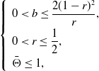 \begin{equation} \left \{ \begin{array}{cc} \begin{aligned} &0\lt b\le \frac{2(1-r)^2}{r},\\ &0\lt r\le \frac{1}{2}, \\ &\bar{\Theta }\le 1,\\ \end{aligned} \end{array}\right . \end{equation}
where
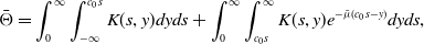 \begin{align*} \bar {\Theta }=\int _{0}^{\infty }\int _{-\infty }^{c_0s}K(s,y)dyds+\int _{0}^{\infty }\int _{c_0s}^{\infty }K(s,y)e^{-\bar {\mu }(c_0s-y)}dyds, \end{align*}
then $c_{\min }=c_0$
.
$c_{\min }=c_0$
.
Proof. We can use part (ii) of Theorem3.5. For illustration, We will alternatively use the upper-lower solution method to prove it. Define a pair of continuous function $(\bar{\Phi }_1, \bar{\Psi }_1)(z)$
as
$(\bar{\Phi }_1, \bar{\Psi }_1)(z)$
as
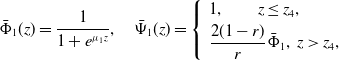 \begin{equation} \bar{\Phi }_1(z)=\frac{1}{1+e^{\mu _1 z}}, \quad \bar{\Psi }_1(z)=\left \{ \begin{array}{cc} \begin{aligned} &1,\quad \quad z\le z_4,\\ &\frac{2(1-r)}{r} \bar{\Phi }_1, \ z\gt z_4,\\ \end{aligned} \end{array}\right . \end{equation}
where $z_4=\frac{1}{\mu _1}\ln \frac{2(1-r)}{r}$
. Let
$z_4=\frac{1}{\mu _1}\ln \frac{2(1-r)}{r}$
. Let $c=c_0+\varepsilon _3$
, where
$c=c_0+\varepsilon _3$
, where $ \varepsilon _3$
is sufficiently small. It follows that
$ \varepsilon _3$
is sufficiently small. It follows that $\mu _1\sim \bar{\mu }=\sqrt{1-r}$
. We shall prove
$\mu _1\sim \bar{\mu }=\sqrt{1-r}$
. We shall prove $(\bar{\Phi }_1, \bar{\Psi }_1)(z)$
is an upper solution of (1.5)-(1.6) under condition (3.32). Substituting
$(\bar{\Phi }_1, \bar{\Psi }_1)(z)$
is an upper solution of (1.5)-(1.6) under condition (3.32). Substituting $(\bar{\Phi }_1, \bar{\Psi }_1)(z)$
into (1.5) gives
$(\bar{\Phi }_1, \bar{\Psi }_1)(z)$
into (1.5) gives
 \begin{align*} \bar {\Psi }_1^{\prime\prime}(z)+c\bar {\Psi }_1^{\prime}(z)+b\bar {\Phi }_1(z)(1-\bar {\Psi }_1(z))=0, \ z\le z_4, \end{align*}
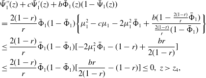 \begin{align*} \begin {aligned} &\bar {\Psi }_1^{\prime\prime}(z)+c\bar {\Psi }_1^{\prime}(z)+b\bar {\Phi }_1(z)(1-\bar {\Psi }_1(z))\\ &=\frac {2(1-r)}{r}\bar {\Phi }_1(1-\bar {\Phi }_1)\bigg \{ \mu _1^2-c\mu _1-2\mu _1^2\bar {\Phi }_1+\frac {b(1-\frac {2(1-r)}{r}\bar {\Phi }_1)}{\frac {2(1-r)}{r}(1-\bar {\Phi }_1)} \bigg \}\\ &\le \frac {2(1-r)}{r}\bar {\Phi }_1(1-\bar {\Phi }_1)[{-}2\mu _1^2\bar {\Phi }_1-(1-r)+\frac {br}{2(1-r)}]\\ &\le \frac {2(1-r)}{r}\bar {\Phi }_1(1-\bar {\Phi }_1)[\frac {br}{2(1-r)}-(1-r)]\le 0, \ z\gt z_4, \end {aligned} \end{align*}
by (3.31), and
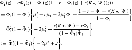 \begin{align*} \begin {aligned} &\bar {\Phi }_1^{\prime\prime}(z)+c\bar {\Phi }_1^{\prime}(z)+\bar {\Phi }_1(z)(1-r-\bar {\Phi }_1(z)+r(K\star _c\bar {\Psi }_1)(z))\\ &=\bar {\Phi }_1(1-\bar {\Phi }_1)\bigg \{ \mu _1^2-c\mu _1-2\mu _1^2\bar {\Phi }_1+\frac {1-r-\bar {\Phi }_1+r(K\star _c\bar {\Psi }_1)}{1-\bar {\Phi }_1} \bigg \}\\ &=\bar {\Phi }_1^2(1-\bar {\Phi }_1)\bigg \{-2\mu _1^2+\frac {r(K\star _c\bar {\Psi }_1)-r\bar {\Phi }_1}{(1-\bar {\Phi }_1)\bar {\Phi }_1} \bigg \}\\ &\,:\!=\,\bar {\Phi }_1^2(1-\bar {\Phi }_1)\bigg \{-2\mu _1^2+J \bigg \}. \end {aligned} \end{align*}
Note that
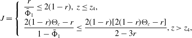 \begin{equation} J=\left \{ \begin{array}{cc} \begin{aligned} &\frac{r}{\bar{\Phi }_1}\le 2(1-r),\ z\le z_4,\\ &\frac{2(1-r)\Theta _c-r}{1-\bar{\Phi }_1}\le \frac{2(1-r)[2(1-r)\Theta _c-r]}{2-3r}, z\gt z_4, \end{aligned} \end{array}\right . \end{equation}
where
 \begin{align*} \Theta _c=\int _{0}^{\infty }\int _{-\infty }^{cs}K(s,y)dyds+\int _{0}^{\infty }\int _{cs}^{\infty }K(s,y)e^{-\mu _1(cs-y)}dyds. \end{align*}
Then $-2\mu _1^2+J \le 0$
by (3.31). Therefore,
$-2\mu _1^2+J \le 0$
by (3.31). Therefore, $(\bar{\Phi }_1, \bar{\Psi }_1)(z)$
is an upper solution of (1.5)-(1.6). By Theorem3.5, we know
$(\bar{\Phi }_1, \bar{\Psi }_1)(z)$
is an upper solution of (1.5)-(1.6). By Theorem3.5, we know $c_{\min }=c_0$
when (3.31) holds. The proof is complete.
$c_{\min }=c_0$
when (3.31) holds. The proof is complete.
Theorem 3.8.
Assume that H2 and (K1) hold. If $b$
and
$b$
and $r$
satisfy
$r$
satisfy
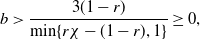 \begin{equation} b\gt \frac{3(1-r)}{\min \{r\chi -(1-r), 1\}}\ge 0, \end{equation}
where
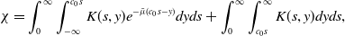 \begin{align*} \chi =\int _{0}^{\infty }\int _{-\infty }^{c_0s}K(s,y)e^{-\bar {\mu }(c_0s-y)}dyds +\int _{0}^{\infty }\int _{c_0s}^{\infty }K(s,y)dyds, \end{align*}
then $c_{\min }\gt c_0$
.
$c_{\min }\gt c_0$
.
Proof. We shall use Theorem3.5 to prove this theorem. The key point is to find a suitable lower solution satisfying all conditions in Theorem3.5. Define a pair of continuous function $(\underline{\Phi }_1, \underline{\Psi }_1)(z)$
as
$(\underline{\Phi }_1, \underline{\Psi }_1)(z)$
as
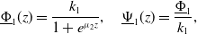 \begin{align*} \underline {\Phi }_1(z)=\frac {k_1}{1+e^{\mu _2 z}},\quad \underline {\Psi }_1(z)=\frac {\underline {\Phi }_1}{k_1}, \end{align*}
where $0\lt k_1\lt 1$
. We need to prove
$0\lt k_1\lt 1$
. We need to prove $(\underline{\Phi }_1, \underline{\Psi }_1)(z)$
is the lower solution of system (1.5)-(1.6). According to (3.34),
$(\underline{\Phi }_1, \underline{\Psi }_1)(z)$
is the lower solution of system (1.5)-(1.6). According to (3.34), $k_1$
can be chosen such that
$k_1$
can be chosen such that
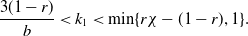 \begin{equation} \frac{3(1-r)}{b}\lt k_1\lt \min \{r\chi -(1-r), 1\}. \end{equation}
We have
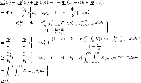 \begin{align*} \begin {aligned} &\underline {\Phi }_1^{\prime\prime}(z)+c\underline {\Phi }_1^{\prime}(z)+\underline {\Phi }_1(z)(1-r-\underline {\Phi }_1(z)+r(K\star _c\underline {\Psi }_1)(z))\\ &=\underline {\Phi }_1(1-\frac {\underline {\Phi }_1}{k_1}) \bigg \{\mu _2^2-c\mu _2+1-r+\frac {\underline {\Phi }_1}{k_1}[{-}2\mu _2^2\\ &+\frac {(1-r)\frac {\underline {\Phi }_1}{k_1}-\underline {\Phi }_1+r\frac {\Phi _1}{k_1}\int _{0}^{\infty }\int _{\mathbb {R}}K(s,y)\frac {1+e^{\mu _2 z}}{1+e^{\mu _2 z}e^{\mu _2(cs-y)}}dyds}{(1-\frac {\underline {\Phi }_1}{k_1})\frac {\underline {\Phi }_1}{k_1}}]\bigg \}\\ &=\frac {\underline {\Phi }_1^2}{k_1}(1-\frac {\underline {\Phi }_1}{k_1})\bigg \{ -2\mu _2^2+\frac {(1-r)-k_1+r\int _{0}^{\infty }\int _{\mathbb {R}}K(s,y)\frac {1+e^{\mu _2 z}}{1+e^{\mu _2 z}e^{\mu _2(cs-y)}}dyds}{1-\frac {\underline {\Phi }_1}{k_1}} \bigg \}\\ &\ge \frac {\underline {\Phi }_1^2}{k_1}(1-\frac {\underline {\Phi }_1}{k_1})\bigg \{ -2\mu _2^2+(1-r)-k_1+r[\int _{0}^{\infty }\int _{-\infty }^{cs}K(s,y)e^{-\mu _2(cs-y)}dyds\\ &+\int _{0}^{\infty }\int _{cs}^{\infty }K(s,y)dyds] \bigg \}\\ &\ge 0, \end {aligned} \end{align*}
and
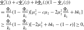 \begin{align*} \begin {aligned} &\underline {\Psi }_1^{\prime\prime}(z)+c\underline {\Psi }_1^{\prime}(z)+b\underline {\Phi }_1(z)(1-\underline {\Psi }_1(z))\\ &=\frac {\underline {\Phi }_1}{k_1}(1-\frac {\underline {\Phi }_1}{k_1})[\mu _2^2-c\mu _2-2\mu _2^2\frac {\underline {\Phi }_1}{k_1}+bk_1]\\ &\ge \frac {\underline {\Phi }_1}{k_1}(1-\frac {\underline {\Phi }_1}{k_1})[{-}2\mu _2^2+bk_1-(1-r)]\ge 0, \end {aligned} \end{align*}
by using (3.35) and $\mu _2\sim \sqrt{1-r}$
for
$\mu _2\sim \sqrt{1-r}$
for $c=c_0+\varepsilon _3$
, where
$c=c_0+\varepsilon _3$
, where $\varepsilon _3\gt 0$
is small. Thus,
$\varepsilon _3\gt 0$
is small. Thus, $(\underline{\Phi }_1, \underline{\Psi }_1)(z)$
is a lower solution of (1.5)-(1.6). It follows that
$(\underline{\Phi }_1, \underline{\Psi }_1)(z)$
is a lower solution of (1.5)-(1.6). It follows that $c_{\min }\gt c_0$
by Theorem3.5. Thus, the proof is complete.
$c_{\min }\gt c_0$
by Theorem3.5. Thus, the proof is complete.
Hasík et al. [Reference Hasík, Kopfová, Nábělková, Trofymchuk and Trofimchuk12] also derived a linear speed selection condition
 \begin{equation} 0\lt b\le \frac{1-r}{r\Theta }, \end{equation}
where
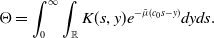 \begin{align*} \Theta =\int _{0}^{\infty }\int _{\mathbb {R}}K(s,y)e^{-\bar {\mu }(c_0s-y)}dyds. \end{align*}
Here, the condition (3.36) can be regards as an estimate for $b^*$
.
$b^*$
.
3.3. The decay behaviour of the travelling wave with the minimal speed
In this subsection, we shall analyse how the travelling wave with the minimal speed decays in different parameter $b$
and
$b$
and $r$
, respectively. The subsequent theorem provides information on the rate at which the travelling wave with the minimal speed decays, with respect to the parameter
$r$
, respectively. The subsequent theorem provides information on the rate at which the travelling wave with the minimal speed decays, with respect to the parameter $b$
. Our aim is to demonstrate that as
$b$
. Our aim is to demonstrate that as $b$
approaches
$b$
approaches $b^*$
from below, the decay rate of the travelling wave with the minimal speed transitions from
$b^*$
from below, the decay rate of the travelling wave with the minimal speed transitions from $ze^{-\mu _1(c_0) z}$
to
$ze^{-\mu _1(c_0) z}$
to $e^{-\mu _1(c_0) z}$
. In previous work by Wu et al. [Reference Wu, Xiao and Zhou41, Theorems 1.2 and 1.5], a similar outcome was established for scalar reaction-diffusion equations and two-species Lotka–Volterra competition systems. However, their approach involved constructing an intricate upper solution, which poses challenges to its applicability to our non-local model. Here, we have developed a novel technique to prove this decay behaviour for this Belousov–Zhabotinsky system with spatiotemporal interaction.
$e^{-\mu _1(c_0) z}$
. In previous work by Wu et al. [Reference Wu, Xiao and Zhou41, Theorems 1.2 and 1.5], a similar outcome was established for scalar reaction-diffusion equations and two-species Lotka–Volterra competition systems. However, their approach involved constructing an intricate upper solution, which poses challenges to its applicability to our non-local model. Here, we have developed a novel technique to prove this decay behaviour for this Belousov–Zhabotinsky system with spatiotemporal interaction.
Theorem 3.9.
Assume that H2 and (K1) hold. Let $b^*$
be the turning point for the minimal speed selection for fixed
$b^*$
be the turning point for the minimal speed selection for fixed $r$
, specifically
$r$
, specifically $c_{\min }=c_0$
for
$c_{\min }=c_0$
for $b \in (0, b^*]$
, and
$b \in (0, b^*]$
, and $c_{\min }\in (c_0,2]$
for
$c_{\min }\in (c_0,2]$
for $b\gt b^*$
. The behaviour of the minimal-speed travelling wave solution
$b\gt b^*$
. The behaviour of the minimal-speed travelling wave solution $(\Phi (z), \Psi (z))$
of system (1.5)-(1.6) can be described as follows:
$(\Phi (z), \Psi (z))$
of system (1.5)-(1.6) can be described as follows:
-
(1) if
$b\in (0, b^*)$
, then
$\Phi (z)\sim Aze^{-\mu _1(c_0) z}$
as
$z\rightarrow \infty$
, where
$A\gt 0$
; -
(2) if
$b=b^*$
, then
$\Phi (z)\sim Be^{-\mu _1(c_0) z}$
as
$z\rightarrow \infty$
, where
$B\gt 0$
; -
(3) if
$b\gt b^*$
, then
$\Phi (z)\sim Be^{-\mu _2(c_{\min }) z}$
as
$z\rightarrow \infty$
, where
$B\gt 0$
.


Proof. Note that $c_{\min }\gt c_0=0$
for all
$c_{\min }\gt c_0=0$
for all $b\gt 0$
when
$b\gt 0$
when $r=1$
. It follows from Theorem3.4 that when
$r=1$
. It follows from Theorem3.4 that when $r=1$
, the result (3) holds for
$r=1$
, the result (3) holds for $b\gt 0$
. Thus, we only consider
$b\gt 0$
. Thus, we only consider $r\in (0,1)$
. For
$r\in (0,1)$
. For $b \in (0, b^*]$
, Theorem3.6 implies
$b \in (0, b^*]$
, Theorem3.6 implies $c_{\min }=c_0$
. Then we have
$c_{\min }=c_0$
. Then we have
 \begin{equation} \Phi (z)\sim Aze^{-\mu _1(c_0) z}+Be^{-\mu _1(c_0) z}, \ \ \text{as} \ z\rightarrow \infty, \end{equation}
where $A\gt 0$
, or
$A\gt 0$
, or $B\gt 0$
if
$B\gt 0$
if $A=0$
, see [Reference Aronson and Weinberger4]. To establish result (2), we utilise a method similar to that employed in Theorem3.4. Denote the minimal-speed travelling wave solution
$A=0$
, see [Reference Aronson and Weinberger4]. To establish result (2), we utilise a method similar to that employed in Theorem3.4. Denote the minimal-speed travelling wave solution $(\Phi (z),\Psi (z))$
by
$(\Phi (z),\Psi (z))$
by $(\Phi ^*(z), \Psi ^*(z))$
for
$(\Phi ^*(z), \Psi ^*(z))$
for $b=b^*$
. Then
$b=b^*$
. Then $(\Phi ^*(z), \Psi ^*(z))$
satisfies
$(\Phi ^*(z), \Psi ^*(z))$
satisfies
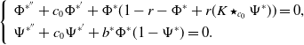 \begin{equation} \left \{ \begin{array}{cc} \begin{aligned} &\Phi ^{*^{\prime\prime}}+c_0\Phi ^{*^{\prime}}+\Phi ^*(1-r-\Phi ^*+r(K\star _{c_0}\Psi ^*))=0,\\ &\Psi ^{*^{\prime\prime}}+c_0\Psi ^{*^{\prime}}+b^*\Phi ^*(1-\Psi ^*)=0.\\ \end{aligned} \end{array}\right . \end{equation}
To the contrary, we assume that $\Phi ^*(z)\sim Aze^{-\mu _1(c_0) z}$
as
$\Phi ^*(z)\sim Aze^{-\mu _1(c_0) z}$
as $z\rightarrow \infty$
with
$z\rightarrow \infty$
with $A\gt 0$
. Consider
$A\gt 0$
. Consider $b_\varepsilon =b^*+\varepsilon$
, where
$b_\varepsilon =b^*+\varepsilon$
, where $\varepsilon$
is sufficiently small to be determined. Let
$\varepsilon$
is sufficiently small to be determined. Let
 \begin{align*}\Phi _\varepsilon (z)=\Phi ^*(z)+W_3(z)\ \text {and} \ \Psi _\varepsilon (z)=\Psi ^*(z)+W_4(z), \end{align*}
where $W_3, W_4 \in B_0=\{u\in C({-}\infty, \infty ), u(\pm \infty )=0\}$
. Our goal is to show the existence of
$W_3, W_4 \in B_0=\{u\in C({-}\infty, \infty ), u(\pm \infty )=0\}$
. Our goal is to show the existence of $W_3$
and
$W_3$
and $W_4$
such that
$W_4$
such that $(\Phi _\varepsilon (z), \Psi _\varepsilon (z))$
satisfies (1.5) with
$(\Phi _\varepsilon (z), \Psi _\varepsilon (z))$
satisfies (1.5) with $b = b_\varepsilon$
and
$b = b_\varepsilon$
and $c = c_0$
. If we can demonstrate this, it would contradict the definition of
$c = c_0$
. If we can demonstrate this, it would contradict the definition of $b^*$
and therefore establish result (2). Suppose that
$b^*$
and therefore establish result (2). Suppose that $(\Phi _\varepsilon (z), \Psi _\varepsilon (z))$
is a solution of (1.5) with
$(\Phi _\varepsilon (z), \Psi _\varepsilon (z))$
is a solution of (1.5) with $b=b_\varepsilon$
and
$b=b_\varepsilon$
and $c=c_0$
. It implies
$c=c_0$
. It implies
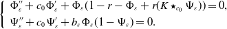 \begin{equation} \left \{ \begin{array}{cc} \begin{aligned} &\Phi _\varepsilon ^{\prime\prime}+c_0\Phi _\varepsilon ^{\prime}+\Phi _\varepsilon (1-r-\Phi _\varepsilon +r(K\star _{c_0}\Psi _\varepsilon ))=0,\\ &\Psi _\varepsilon ^{\prime\prime}+c_0\Psi _\varepsilon ^{\prime}+b_{\varepsilon }\Phi _\varepsilon (1-\Psi _\varepsilon )=0.\\ \end{aligned} \end{array}\right . \end{equation}
By (3.38) and (3.39), $W_3$
and
$W_3$
and $W_4$
satisfy
$W_4$
satisfy
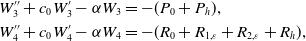 \begin{equation} \begin{aligned} &W_3^{\prime\prime}+c_0W_3^{\prime}-\alpha W_3=-(P_0+P_h),\\ &W_4^{\prime\prime}+c_0W_4^{\prime}-\alpha W_4=-(R_0+R_{1,\varepsilon }+R_{2,\varepsilon }+R_h), \end{aligned} \end{equation}
where
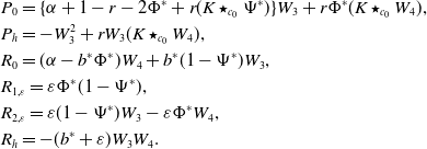 \begin{align*} \begin {aligned} &P_0=\{ \alpha +1-r-2\Phi ^*+r(K\star _{c_0}\Psi ^*)\}W_3+r\Phi ^*(K\star _{c_0} W_4),\\ &P_h=-W_3^2+rW_3(K\star _{c_0} W_4),\\ &R_0=( \alpha -b^*\Phi ^*)W_4+b^*(1-\Psi ^*)W_3,\\ &R_{1,\varepsilon }=\varepsilon \Phi ^*(1-\Psi ^*),\\ &R_{2,\varepsilon }=\varepsilon (1-\Psi ^*)W_3-\varepsilon \Phi ^*W_4,\\ &R_h=-(b^*+\varepsilon )W_3W_4.\\ \end {aligned} \end{align*}
Therefore, for $c=c_0$
, we have
$c=c_0$
, we have
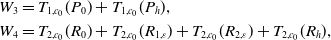 \begin{equation} \begin{aligned} &W_3=T_{1,c_0}(P_0)+T_{1,c_0}(P_h),\\ &W_4=T_{2,c_0}(R_0)+T_{2,c_0}(R_{1,\varepsilon })+T_{2,c_0}(R_{2,\varepsilon })+T_{2,c_0}(R_h), \end{aligned} \end{equation}
where $T_{1,c_0}$
and
$T_{1,c_0}$
and $T_{2,c_0}$
are defined in (3.28). Define
$T_{2,c_0}$
are defined in (3.28). Define
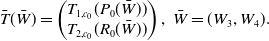 \begin{align*} \bar {T}(\bar {W})= \begin {pmatrix} T_{1,c_0}(P_0(\bar {W}))\\ T_{2,c_0}(R_0(\bar {W})) \end {pmatrix}, \ \bar {W}=(W_3, W_4). \end{align*}
Clearly, $T_{2,c_0}(R_{1,\varepsilon })=O(\varepsilon )$
and
$T_{2,c_0}(R_{1,\varepsilon })=O(\varepsilon )$
and $T_{2,c_0}(R_{2,\varepsilon })=O(\varepsilon \bar{W})$
. The linear operator
$T_{2,c_0}(R_{2,\varepsilon })=O(\varepsilon \bar{W})$
. The linear operator $\bar{T}$
is both compact and strongly positive, and it possesses a simple principal eigenvalue
$\bar{T}$
is both compact and strongly positive, and it possesses a simple principal eigenvalue $\lambda =1$
associated with the positive eigenfunction
$\lambda =1$
associated with the positive eigenfunction $({-}\Phi ^{*^{\prime}},-\Psi ^{*^{\prime}})$
. To eliminate this eigenfunction from
$({-}\Phi ^{*^{\prime}},-\Psi ^{*^{\prime}})$
. To eliminate this eigenfunction from $B_0$
, we introduce a weighted functional space defined as
$B_0$
, we introduce a weighted functional space defined as
 \begin{align*}\mathcal {H}_2=\{h(\xi )\in B_0\ :\ he^{\mu _1(c_0)\xi }=o(1) \quad \rm {as} \quad \xi \rightarrow \infty \}.\end{align*}
Since $({-}\Phi ^{*^{\prime}},-\Psi ^{*^{\prime}})$
does not belong to the space
$({-}\Phi ^{*^{\prime}},-\Psi ^{*^{\prime}})$
does not belong to the space $\mathcal{H}_2\times B_0$
, it follows that
$\mathcal{H}_2\times B_0$
, it follows that $\bar{T}$
does not possess the eigenvalue
$\bar{T}$
does not possess the eigenvalue $\lambda =1$
for
$\lambda =1$
for $(W_3,W_4)$
in
$(W_3,W_4)$
in $\mathcal{H}_2\times B_0$
. In other words,
$\mathcal{H}_2\times B_0$
. In other words, $I-\bar{T}$
(where
$I-\bar{T}$
(where $I$
denotes the identity operator) has a bounded inverse in
$I$
denotes the identity operator) has a bounded inverse in $\mathcal{H}_2\times B_0$
. Consequently, there exists a solution
$\mathcal{H}_2\times B_0$
. Consequently, there exists a solution $(W_3,W_4)$
to (3.41) for any
$(W_3,W_4)$
to (3.41) for any $\varepsilon \in [0, \varepsilon _0)$
, where
$\varepsilon \in [0, \varepsilon _0)$
, where $\varepsilon _0$
is a small positive number. This implies that there exists a
$\varepsilon _0$
is a small positive number. This implies that there exists a $\varepsilon _0$
such that the solution
$\varepsilon _0$
such that the solution $(\Phi _\varepsilon, \Psi _\varepsilon )$
to (1.5)-(1.6) exists with
$(\Phi _\varepsilon, \Psi _\varepsilon )$
to (1.5)-(1.6) exists with $c=c_0$
for
$c=c_0$
for $b=b_\varepsilon =b^*+\varepsilon \lt b^*+\varepsilon _0$
. However, this contradicts the conclusion in Theorem3.6. Thus, result (2) holds true.
$b=b_\varepsilon =b^*+\varepsilon \lt b^*+\varepsilon _0$
. However, this contradicts the conclusion in Theorem3.6. Thus, result (2) holds true.
We can establish result (1) using a similar approach as presented in [Reference Wu, Xiao and Zhou41, Theorem 1.2]. Suppose there exists $b\in (0, b^*)$
such that the minimal-speed travelling wave solution satisfies
$b\in (0, b^*)$
such that the minimal-speed travelling wave solution satisfies
 \begin{equation} \Phi _b(z)\sim B_1e^{-\mu _1(c_0)z},\ \text{as} \ z\rightarrow \infty, \ B_1\gt 0. \end{equation}
Then by asymptotic analysis, we have
 \begin{align*} \Psi _b(z)\sim B_2e^{-\mu _1(c_0)z},\ \text {as} \ z\rightarrow \infty, \ B_2\gt 0. \end{align*}
By result (2), for $b=b^*$
, the minimal-speed travelling wave
$b=b^*$
, the minimal-speed travelling wave $(\Phi _{b^*}, \Psi _{b^*})$
satisfies
$(\Phi _{b^*}, \Psi _{b^*})$
satisfies
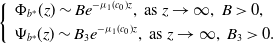 \begin{equation} \left \{\begin{array}{cc} \begin{aligned} &\Phi _{b^*}(z)\sim Be^{-\mu _1(c_0)z}, \ \text{as} \ z\rightarrow \infty, \ B\gt 0,\\ &\Psi _{b^*}(z)\sim B_3e^{-\mu _1(c_0)z}, \ \text{as} \ z\rightarrow \infty, \ B_3\gt 0. \end{aligned} \end{array}\right . \end{equation}
As $z\rightarrow -\infty$
, we obtain
$z\rightarrow -\infty$
, we obtain
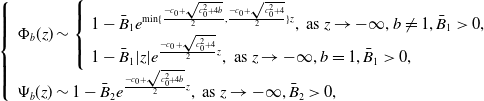 \begin{align*} \left \{\begin {array}{cc} \begin {aligned} &\Phi _b(z)\sim \left \{ \begin {array}{cc} \begin {aligned} &1-\bar {B}_1e^{\min \{\frac {-c_0+\sqrt {c_0^2+4b}}{2}, \frac {-c_0+\sqrt {c_0^2+4}}{2}\} z},\ \text {as} \ z\rightarrow -\infty, b\neq 1, \bar {B}_1\gt 0,\\ &1-\bar {B}_1|z|e^{ \frac {-c_0+\sqrt {c_0^2+4}}{2} z }, \ \text {as} \ z\rightarrow -\infty, b=1, \bar {B}_1\gt 0, \\ \end {aligned} \end {array}\right . \\ &\Psi _b(z)\sim 1-\bar {B}_2e^{ \frac {-c_0+\sqrt {c_0^2+4b}}{2} z },\ \text {as} \ z\rightarrow -\infty, \bar {B}_2\gt 0, \end {aligned} \end {array}\right . \end{align*}
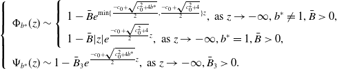 \begin{align*} \left \{\begin {array}{cc} \begin {aligned} &\Phi _{b^*}(z)\sim \left \{ \begin {array}{cc} \begin {aligned} &1-\bar {B}e^{\min \{\frac {-c_0+\sqrt {c_0^2+4b^*}}{2}, \frac {-c_0+\sqrt {c_0^2+4}}{2}\} z},\ \text {as} \ z\rightarrow -\infty, b^*\neq 1, \bar {B}\gt 0,\\ &1-\bar {B}|z|e^{ \frac {-c_0+\sqrt {c_0^2+4}}{2} z }, \ \text {as} \ z\rightarrow -\infty, b^*=1, \bar {B}\gt 0, \\ \end {aligned} \end {array}\right . \\ &\Psi _{b^*}(z)\sim 1-\bar {B}_3e^{ \frac {-c_0+\sqrt {c_0^2+4b^*}}{2} z },\ \text {as} \ z\rightarrow -\infty, \bar {B}_3\gt 0. \end {aligned} \end {array}\right . \end{align*}
Consequently, there exists an $L\gt 0$
such that
$L\gt 0$
such that $\Phi _{b^*}(z-L)\gt \Phi _b(z)$
and
$\Phi _{b^*}(z-L)\gt \Phi _b(z)$
and $\Psi _{b^*}(z-L)\gt \Psi _b(z)$
for all
$\Psi _{b^*}(z-L)\gt \Psi _b(z)$
for all $z\in \mathbb{R}$
. Define
$z\in \mathbb{R}$
. Define
 \begin{align*} L^*\,:\!=\,\inf \{L\in \mathbb {R}| \Phi _{b^*}(z-L)\ge \Phi _b(z), \ \Psi _{b^*}(z-L)\ge \Psi _b(z), \ \forall z\in \mathbb {R}\}. \end{align*}
Suppose there exists $z_1\in \mathbb{R}$
such that
$z_1\in \mathbb{R}$
such that $\Phi _{b^*}(z_1-L^*)=\Phi _b(z_1)$
. By the strong maximum principle, it follows that
$\Phi _{b^*}(z_1-L^*)=\Phi _b(z_1)$
. By the strong maximum principle, it follows that $\Phi _{b^*}(z-L^*)=\Phi _b(z)$
for all
$\Phi _{b^*}(z-L^*)=\Phi _b(z)$
for all $z\in \mathbb{R}$
. However, this contradicts the fact that
$z\in \mathbb{R}$
. However, this contradicts the fact that $(\Phi _{b^*}(z-L^*), \Psi _{b^*}(z-L^*) )$
and
$(\Phi _{b^*}(z-L^*), \Psi _{b^*}(z-L^*) )$
and $(\Phi _b(z),\Psi _b(z))$
satisfy different equations. Thus,
$(\Phi _b(z),\Psi _b(z))$
satisfy different equations. Thus, $\Phi _{b^*}(z-L^*)\gt \Phi _b(z)$
for all
$\Phi _{b^*}(z-L^*)\gt \Phi _b(z)$
for all $z\in \mathbb{R}$
. Similarly, we can prove
$z\in \mathbb{R}$
. Similarly, we can prove $\Psi _{b^*}(z-L^*)\gt \Psi _b(z)$
for all
$\Psi _{b^*}(z-L^*)\gt \Psi _b(z)$
for all $z\in \mathbb{R}$
.
$z\in \mathbb{R}$
.
Based on the above argument, we claim that
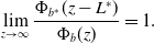 \begin{equation} \lim \limits _{z\rightarrow \infty } \frac{\Phi _{b^*}(z-L^*)}{\Phi _b(z)}=1. \end{equation}
Assuming $\lim \limits _{z\rightarrow \infty } \frac{\Phi _{b^*}(z-L^*)}{\Phi _b(z)}\gt 1$
, then by the second equation in (1.5), we can deduce that
$\lim \limits _{z\rightarrow \infty } \frac{\Phi _{b^*}(z-L^*)}{\Phi _b(z)}\gt 1$
, then by the second equation in (1.5), we can deduce that $\lim \limits _{z\rightarrow \infty } \frac{\Psi _{b^*}(z-L^*)}{\Psi _b(z)}\gt 1$
. Therefore, there exists a sufficiently small
$\lim \limits _{z\rightarrow \infty } \frac{\Psi _{b^*}(z-L^*)}{\Psi _b(z)}\gt 1$
. Therefore, there exists a sufficiently small $\varepsilon _1\gt 0$
such that
$\varepsilon _1\gt 0$
such that $\Phi _{b^*}(z-(L^*-\varepsilon _1))\ge \Phi _b(z)$
and
$\Phi _{b^*}(z-(L^*-\varepsilon _1))\ge \Phi _b(z)$
and $\Psi _{b^*}(z-(L^*-\varepsilon _1))\ge \Psi _b(z)$
for
$\Psi _{b^*}(z-(L^*-\varepsilon _1))\ge \Psi _b(z)$
for $z\in \mathbb{R}$
. However, this contradicts the definition of
$z\in \mathbb{R}$
. However, this contradicts the definition of $L^*$
. Hence, the claim (3.44) holds.
$L^*$
. Hence, the claim (3.44) holds.
With the established claim, we have $Be^{\mu _1(c_0)L^*}=B_1$
. Let
$Be^{\mu _1(c_0)L^*}=B_1$
. Let $\hat{W}(z)=\Phi _{b^*}(z-L^*)-\Phi _b(z)$
. Then
$\hat{W}(z)=\Phi _{b^*}(z-L^*)-\Phi _b(z)$
. Then $\hat{W}(z)$
satisfies
$\hat{W}(z)$
satisfies
 \begin{equation} \hat{W}^{\prime\prime}+c_0\hat{W}^{\prime}+G_1(b^*, c_0, \Phi _{b^*}(z-L^*),\Psi _{b^*}(z-L^*))-G_1(b, c_0, \Phi _b(z), \Psi _b(z))=0, \end{equation}
where
 \begin{align*} G_1(b,c,\Phi, \Psi )=\Phi (1-r-\Phi +r(K\star _c \Psi )). \end{align*}
Note that
 \begin{align*} \hat {W}(z)\sim (Dz+E)e^{-\mu _1(c_0) z}, \ \text {as} \ z\rightarrow \infty, \end{align*}
where $D\ge 0$
, or
$D\ge 0$
, or $E\gt 0$
if
$E\gt 0$
if $D=0$
. By (3.42), (3.43), and
$D=0$
. By (3.42), (3.43), and $Be^{\mu _1(c_0)L^*}=B_1$
, we know
$Be^{\mu _1(c_0)L^*}=B_1$
, we know $E=0$
and
$E=0$
and $D=0$
. This leads to a contradiction. Thus, result (1) holds.
$D=0$
. This leads to a contradiction. Thus, result (1) holds.
Result (3) can be obtained by combining Theorems3.4 and 3.6. Therefore, the proof is complete.
Similarly, we can consider the decay details of the minimal-speed wave solution based on different $r$
. To this end, we first offer a necessary and sufficient condition based on
$r$
. To this end, we first offer a necessary and sufficient condition based on $r$
when
$r$
when $b$
is fixed.
$b$
is fixed.
Theorem 3.10.
Assume that H2 and (K1) hold. For fixed $b$
, there exists a unique turning point
$b$
, there exists a unique turning point $r^*\in (0,1)$
for the minimal speed selection, that is,
$r^*\in (0,1)$
for the minimal speed selection, that is, $c_{\min }=c_0$
for
$c_{\min }=c_0$
for $r \in (0, r^*]$
, and
$r \in (0, r^*]$
, and $c_{\min }\in (c_0, 2]$
for
$c_{\min }\in (c_0, 2]$
for $r\in (r^*, 1]$
.
$r\in (r^*, 1]$
.
Proof. Since $\Phi$
-equation in system (1.5) becomes the Fisher–Kpp equation when
$\Phi$
-equation in system (1.5) becomes the Fisher–Kpp equation when $r=0$
. That means
$r=0$
. That means $c_{\min }=c_0=2$
, which can be seen in [Reference Kolmogoroff, Petrovsky and Piscounoff17]. Since
$c_{\min }=c_0=2$
, which can be seen in [Reference Kolmogoroff, Petrovsky and Piscounoff17]. Since $c_{\min }$
is non-increasing in
$c_{\min }$
is non-increasing in $r$
by Theorem3.3, we have
$r$
by Theorem3.3, we have $c_{\min }\in [c_0,2]$
when
$c_{\min }\in [c_0,2]$
when $r\in (0,1]$
. When
$r\in (0,1]$
. When $r=1$
, we know
$r=1$
, we know $c_{\min }\gt c_0$
by Theorem3.8. Therefore, there exists at least one turning point
$c_{\min }\gt c_0$
by Theorem3.8. Therefore, there exists at least one turning point $r^*$
at which speed selection changes from linearly selected to nonlinearly selected. We shall prove the uniqueness of the turning point
$r^*$
at which speed selection changes from linearly selected to nonlinearly selected. We shall prove the uniqueness of the turning point $r^*$
by contradiction. Let
$r^*$
by contradiction. Let $r_1^*, r_2^*\in (0,1)$
be two turning points for speed selection.
$r_1^*, r_2^*\in (0,1)$
be two turning points for speed selection.
For $r\in [0,1)$
, we shall rewrite system (1.2) by the scaling
$r\in [0,1)$
, we shall rewrite system (1.2) by the scaling
 \begin{align*} x\sqrt {1-r} \rightarrow x, \quad (1-r)t\rightarrow t,\quad \phi (t,x)\rightarrow \phi (t,x),\quad \psi (t,x)\rightarrow \psi (t,x). \end{align*}
Let $(\phi, \psi )=(\Phi, \Psi )(\nu\ {\cdot}\ x-ct)$
, where
$(\phi, \psi )=(\Phi, \Psi )(\nu\ {\cdot}\ x-ct)$
, where $||\nu ||=1$
. Then we have the following wavefront system
$||\nu ||=1$
. Then we have the following wavefront system
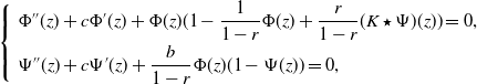 \begin{equation} \left \{ \begin{array}{cc} \begin{aligned} &\Phi ^{\prime\prime}(z)+c\Phi ^{\prime}(z)+\Phi (z)(1-\frac{1}{1-r}\Phi (z)+\frac{r}{1-r}(K\star \Psi )(z))=0,\\ &\Psi ^{\prime\prime}(z)+c\Psi ^{\prime}(z)+\frac{b}{1-r}\Phi (z)(1-\Psi (z))=0,\\ \end{aligned} \end{array} \right . \end{equation}
with the boundary condition (1.6), where
 \begin{align*} (K\star \Psi )(z)= \int _{0}^{+\infty }\int _{\mathbb {R}}K(s,y)\Psi (z+(1-r)cs-\sqrt {1-r}y)dyds. \end{align*}
Linearising (3.46) at $e_0$
, we can get the characteristic equation
$e_0$
, we can get the characteristic equation $\mu ^2-c\mu +1=0$
, which yields two roots
$\mu ^2-c\mu +1=0$
, which yields two roots
 \begin{equation} \mu _3=\mu _3(c)=\frac{c-\sqrt{c^2-4}}{2},\quad \mu _4=\mu _4(c)=\frac{c+\sqrt{c^2-4}}{2}. \end{equation}
Here, the linear speed $\bar{c}_0=2$
.
$\bar{c}_0=2$
.
Let $(r_1^*, \Phi _1, \Psi _1)$
and
$(r_1^*, \Phi _1, \Psi _1)$
and $(r_2^*, \Phi _2, \Psi _2)$
be two solutions of (3.46)-(1.6). According to a similar argument in the proof of Theorem3.9 (2), we know
$(r_2^*, \Phi _2, \Psi _2)$
be two solutions of (3.46)-(1.6). According to a similar argument in the proof of Theorem3.9 (2), we know
 \begin{align*} \begin {aligned} &\Phi _1(z)\sim A_3e^{-\mu _3(\bar {c}_0)z},\ \text {as} \ z\rightarrow \infty, \ A_3\gt 0, \\ &\Phi _2(z)\sim A_4e^{-\mu _3(\bar {c}_0)z},\ \text {as} \ z\rightarrow \infty, \ A_4\gt 0. \end {aligned} \end{align*}
By asymptotic analysis, we have
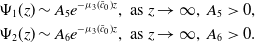 \begin{align*} \begin {aligned} &\Psi _1(z)\sim A_5e^{-\mu _3(\bar {c}_0)z},\ \text {as} \ z\rightarrow \infty, \ A_5\gt 0,\\ &\Psi _2(z)\sim A_6e^{-\mu _3(\bar {c}_0)z},\ \text {as} \ z\rightarrow \infty, \ A_6\gt 0. \end {aligned} \end{align*}
As $z\rightarrow -\infty$
, we obtain
$z\rightarrow -\infty$
, we obtain
 \begin{align*} \left \{\begin {array}{cc} \begin {aligned} &\Phi _1(z)\sim \left \{ \begin {array}{cc} \begin {aligned} &1-\bar {A}_3e^{\min \{\frac {-\bar {c}_0+\sqrt {\bar {c}_0^2+\frac {4b}{1-r_1^*}}}{2}, \frac {-\bar {c}_0+\sqrt {\bar {c}_0^2+\frac {4}{1-r_1^*}}}{2}\} z},\ \text {as} \ z\rightarrow -\infty, b\neq 1, \bar {A}_3\gt 0,\\ &1-\bar {A}_3|z|e^{ \frac {-\bar {c}_0+\sqrt {\bar {c}_0^2+\frac {4}{1-r_1^*}}}{2} z }, \ \text {as} \ z\rightarrow -\infty, b=1, \bar {A}_3\gt 0, \\ \end {aligned} \end {array}\right . \\ &\Psi _1(z)\sim 1-\bar {A}_5e^{ \frac {-\bar {c}_0+\sqrt {\bar {c}_0^2+\frac {4b}{1-r_1^*}}}{2} z },\ \text {as} \ z\rightarrow -\infty, \bar {A}_5\gt 0, \end {aligned} \end {array}\right . \end{align*}
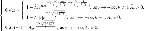 \begin{align*} \left \{\begin {array}{cc} \begin {aligned} &\Phi _2(z)\sim \left \{ \begin {array}{cc} \begin {aligned} &1-\bar {A}_4e^{\min \{\frac {-\bar {c}_0+\sqrt {\bar {c}_0^2+\frac {4b}{1-r_2^*}}}{2}, \frac {-\bar {c}_0+\sqrt {\bar {c}_0^2+\frac {4}{1-r_2^*}}}{2}\} z},\ \text {as} \ z\rightarrow -\infty, b\neq 1, \bar {A}_4\gt 0,\\ &1-\bar {A}_4|z|e^{ \frac {-\bar {c}_0+\sqrt {\bar {c}_0^2+\frac {4}{1-r_2^*}}}{2} z }, \ \text {as} \ z\rightarrow -\infty, b=1, \bar {A}_4\gt 0, \\ \end {aligned} \end {array}\right . \\ &\Psi _2(z)\sim 1-\bar {A}_6e^{ \frac {-\bar {c}_0+\sqrt {\bar {c}_0^2+\frac {4b}{1-r_2^*}}}{2} z },\ \text {as} \ z\rightarrow -\infty, \bar {A}_6\gt 0, \end {aligned} \end {array}\right . \end{align*}
Consequently, there exists an $L\gt 0$
such that
$L\gt 0$
such that $\Phi _{b^*}(z-L)\gt \Phi _b(z)$
and
$\Phi _{b^*}(z-L)\gt \Phi _b(z)$
and $\Psi _{b^*}(z-L)\gt \Psi _b(z)$
for all
$\Psi _{b^*}(z-L)\gt \Psi _b(z)$
for all $z\in \mathbb{R}$
. Define
$z\in \mathbb{R}$
. Define
 \begin{align*} L_1^*\,:\!=\,\inf \{L\in \mathbb {R}| \Phi _2(z-L)\ge \Phi _1(z), \ \Psi _2(z-L)\ge \Psi _1(z), \ \forall z\in \mathbb {R}\}. \end{align*}
By a similar analysis in the proof of Theorem3.9 (1), we will derive a contradiction. Therefore, there exists a unique turning point $r^*$
for speed selection. Hence, the proof is complete.
$r^*$
for speed selection. Hence, the proof is complete.
Based on the above Theorem3.10, we give the decay details of the minimal-speed wave solution of (3.46)-(1.6) based on different $r$
. Since the proof of this assertion is identical to the proof of Theorem3.9, we omit it here.
$r$
. Since the proof of this assertion is identical to the proof of Theorem3.9, we omit it here.
Theorem 3.11.
Assume that H2 and (K1) hold. For fixed $b$
, we let
$b$
, we let $r^*\lt 1$
be the turning point for speed selection of (3.46)-(1.6), that is,
$r^*\lt 1$
be the turning point for speed selection of (3.46)-(1.6), that is, $c_{\min }=\bar{c}_0$
for
$c_{\min }=\bar{c}_0$
for $r \in (0, r^*]$
, and
$r \in (0, r^*]$
, and $c_{\min }\gt \bar{c}_0$
for
$c_{\min }\gt \bar{c}_0$
for $r\in (r^*, 1)$
. The minimal-speed travelling wave solution
$r\in (r^*, 1)$
. The minimal-speed travelling wave solution $(\Phi (z), \Psi (z))$
of system (3.46)-(1.6) satisfies:
$(\Phi (z), \Psi (z))$
of system (3.46)-(1.6) satisfies:
-
(1) if
$r\in (0, r^*)$
, then
$\Phi (z)\sim Aze^{-\mu _3(\bar{c}_0) z}$
as
$z\rightarrow \infty$
, where
$A\gt 0$
; -
(2) if
$r=r^*$
, then
$\Phi (z)\sim Be^{-\mu _3(\bar{c}_0) z}$
as
$z\rightarrow \infty$
, where
$B\gt 0$
; -
(3) if
$r\in (r^*, 1)$
, then
$\Phi (z)\sim Be^{-\mu _4(c_{\min }) z}$
as
$z\rightarrow \infty$
, where
$B\gt 0$
.


4. Numerical analysis
In this section, we will use MATLAB software to simulate our model (1.2) under cases H1-H2 and provide several examples to demonstrate our numerical findings. We consider system (1.2) in $x\in \mathbb{R}$
and choose the kernel function as
$x\in \mathbb{R}$
and choose the kernel function as
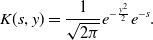 \begin{equation} K(s,y)=\frac{1}{\sqrt{2\pi }}e^{-\frac{y^2}{2}}e^{-s}. \end{equation}
Clearly, conditions (K1) and (K2) hold. We construct the initial conditions of (1.2) as
 \begin{equation} \phi (\theta, x)=\frac{0.5}{1+e^x}, \quad \psi (\theta, x)=\frac{0.5}{1+e^x}, \ \ x\in \mathbb{R},\ \ \theta \in [{-}10,0]. \end{equation}
to calculate the numerical speeds. Although they are not semi-compact supported, the exponentiate decay rate is not smaller than $\sqrt{1-r}$
when
$\sqrt{1-r}$
when $z\rightarrow \infty$
so that the solution still evolves to the wave with minimal speed (see [Reference Hamel and Nadin11, Reference Uchiyama38]). Here we take
$z\rightarrow \infty$
so that the solution still evolves to the wave with minimal speed (see [Reference Hamel and Nadin11, Reference Uchiyama38]). Here we take $\theta \in [{-}10,0]$
in the initial data since the integral
$\theta \in [{-}10,0]$
in the initial data since the integral $\int _{10}^{\infty }\int _{\mathbb{R}}K(s,y)\psi (t-s,x-y)dyds\lt e^{-10}\simeq 4.5\times 10^{-5}$
is very small in the reaction term of system (1.2) when the delay
$\int _{10}^{\infty }\int _{\mathbb{R}}K(s,y)\psi (t-s,x-y)dyds\lt e^{-10}\simeq 4.5\times 10^{-5}$
is very small in the reaction term of system (1.2) when the delay $s\gt 10$
.
$s\gt 10$
.
Example 4.1.
Let $b=1$
and
$b=1$
and $ r=1.2$
. The kernel function and the initial data are defined in (4.1) and (4.2), respectively.
$ r=1.2$
. The kernel function and the initial data are defined in (4.1) and (4.2), respectively.
Since $r=1.2\gt 1$
, this example corresponds to the bistable case H1. The evolution of
$r=1.2\gt 1$
, this example corresponds to the bistable case H1. The evolution of $\phi$
and
$\phi$
and $\psi$
is depicted in Figure 1. In the case H1, both
$\psi$
is depicted in Figure 1. In the case H1, both $e_{\beta }$
and
$e_{\beta }$
and $e_0$
are stable. As illustrated in Figure 1, the solution progresses towards the right (i.e.
$e_0$
are stable. As illustrated in Figure 1, the solution progresses towards the right (i.e. $c\gt 0$
), indicating that bromide ion within the system persists as time
$c\gt 0$
), indicating that bromide ion within the system persists as time $t$
is large.
$t$
is large.
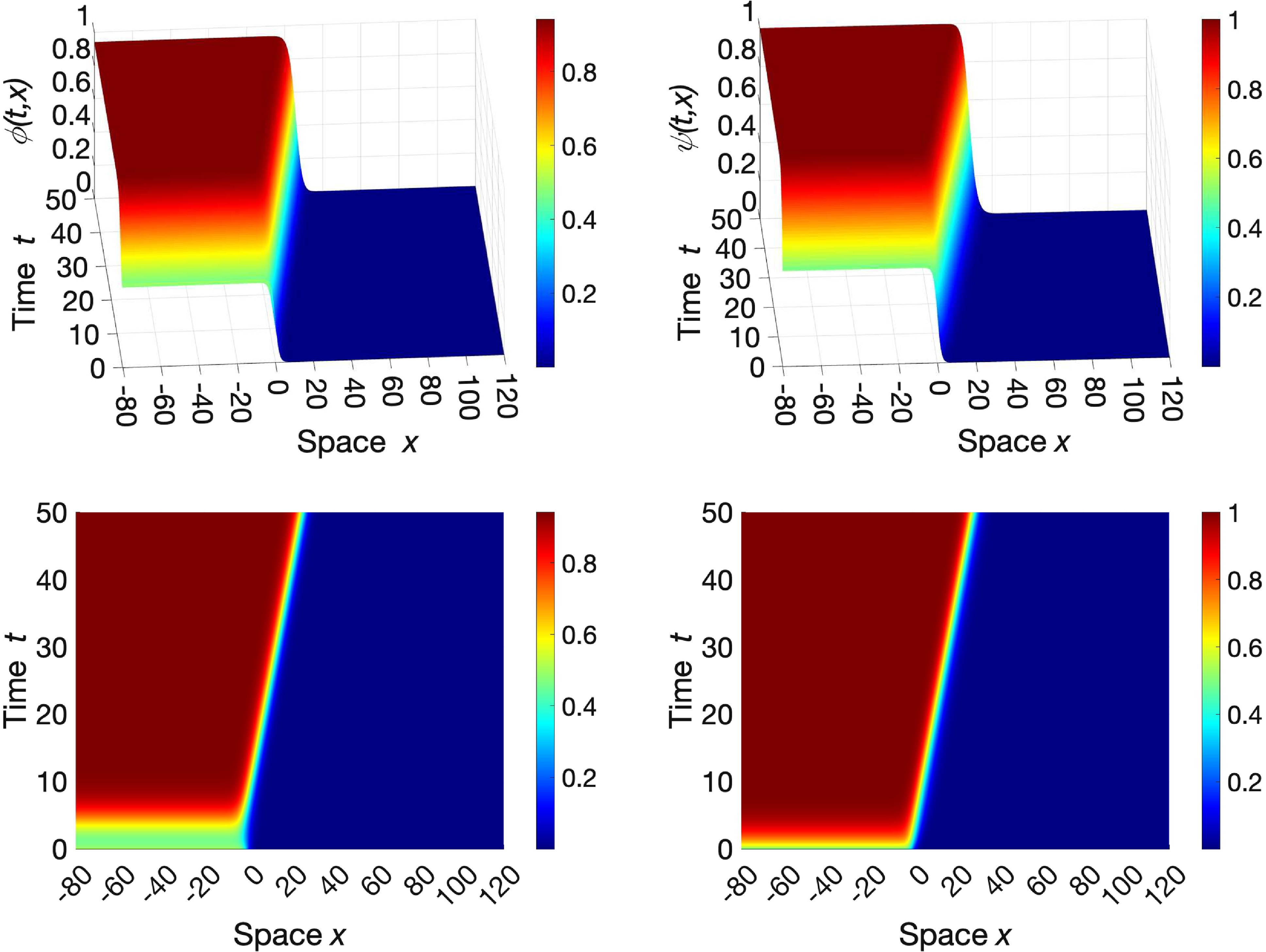
Figure 1. Simulation of $(\phi, \psi )(t,x)$
in accordance with case H1, where the parameters are defined as
$(\phi, \psi )(t,x)$
in accordance with case H1, where the parameters are defined as $b=1$
and
$b=1$
and $r=1.2$
. The first row depicts the spatiotemporal movements of
$r=1.2$
. The first row depicts the spatiotemporal movements of $\phi$
and
$\phi$
and $\psi$
, respectively. The bottom row displays their respective 2-D plots observed from a top view.
$\psi$
, respectively. The bottom row displays their respective 2-D plots observed from a top view.
Example 4.2.
Let $b=5$
and
$b=5$
and $r=0.5$
. The kernel function and the initial data are defined in (4.1) and (4.2), respectively.
$r=0.5$
. The kernel function and the initial data are defined in (4.1) and (4.2), respectively.
In this case, we have $r=0.5\lt 1$
, and then H2 holds. The detailed simulations are presented in Figure 2. These figures clearly demonstrate that the solution propagates to the right, stablising to a constant speed, consistent with the findings when
$r=0.5\lt 1$
, and then H2 holds. The detailed simulations are presented in Figure 2. These figures clearly demonstrate that the solution propagates to the right, stablising to a constant speed, consistent with the findings when $e_{\beta }$
is stable and
$e_{\beta }$
is stable and $e_0$
is unstable under H2. To calculate the numerical speeds, we utilise the level sets depicted in Figure 3. For the computation of the numerical moving speed
$e_0$
is unstable under H2. To calculate the numerical speeds, we utilise the level sets depicted in Figure 3. For the computation of the numerical moving speed $c_{\phi }^*$
of
$c_{\phi }^*$
of $\phi (t,x)$
, we locate the level set
$\phi (t,x)$
, we locate the level set $x(t)$
such that
$x(t)$
such that $\phi (t,x(t))=0.5$
for different values of
$\phi (t,x(t))=0.5$
for different values of $t$
. Similarly, we determine
$t$
. Similarly, we determine $x(t)$
such that
$x(t)$
such that $\psi (t,x(t))=0.5$
to compute the numerical moving speed
$\psi (t,x(t))=0.5$
to compute the numerical moving speed $c_{\psi }^*$
of
$c_{\psi }^*$
of $\psi (t,x)$
. By calculating the difference in
$\psi (t,x)$
. By calculating the difference in $x$
coordinates in the level set and dividing it by the corresponding time difference at each snapshot time, we can obtain the numerical speed. Taking snapshots of
$x$
coordinates in the level set and dividing it by the corresponding time difference at each snapshot time, we can obtain the numerical speed. Taking snapshots of $\phi$
and
$\phi$
and $\psi$
at
$\psi$
at $t=40,41,42,\ldots 50$
(shown in Figure 3), we can derive the moving speeds at different times. Once the speed difference among them becomes less than
$t=40,41,42,\ldots 50$
(shown in Figure 3), we can derive the moving speeds at different times. Once the speed difference among them becomes less than $5\times 10^{-3}$
, we stop the computation and consider their values as the final result. Through this computation, we find that
$5\times 10^{-3}$
, we stop the computation and consider their values as the final result. Through this computation, we find that $c_{\phi }^*=1.4140$
and
$c_{\phi }^*=1.4140$
and $c_{\psi }^*=1.4143$
. Note that the linear speed
$c_{\psi }^*=1.4143$
. Note that the linear speed $c_0=2\sqrt{1-r}=1.4142$
. Therefore, we conclude that
$c_0=2\sqrt{1-r}=1.4142$
. Therefore, we conclude that $c_{\phi }^*\simeq c_{\psi }^*\simeq c_0$
.
$c_{\phi }^*\simeq c_{\psi }^*\simeq c_0$
.
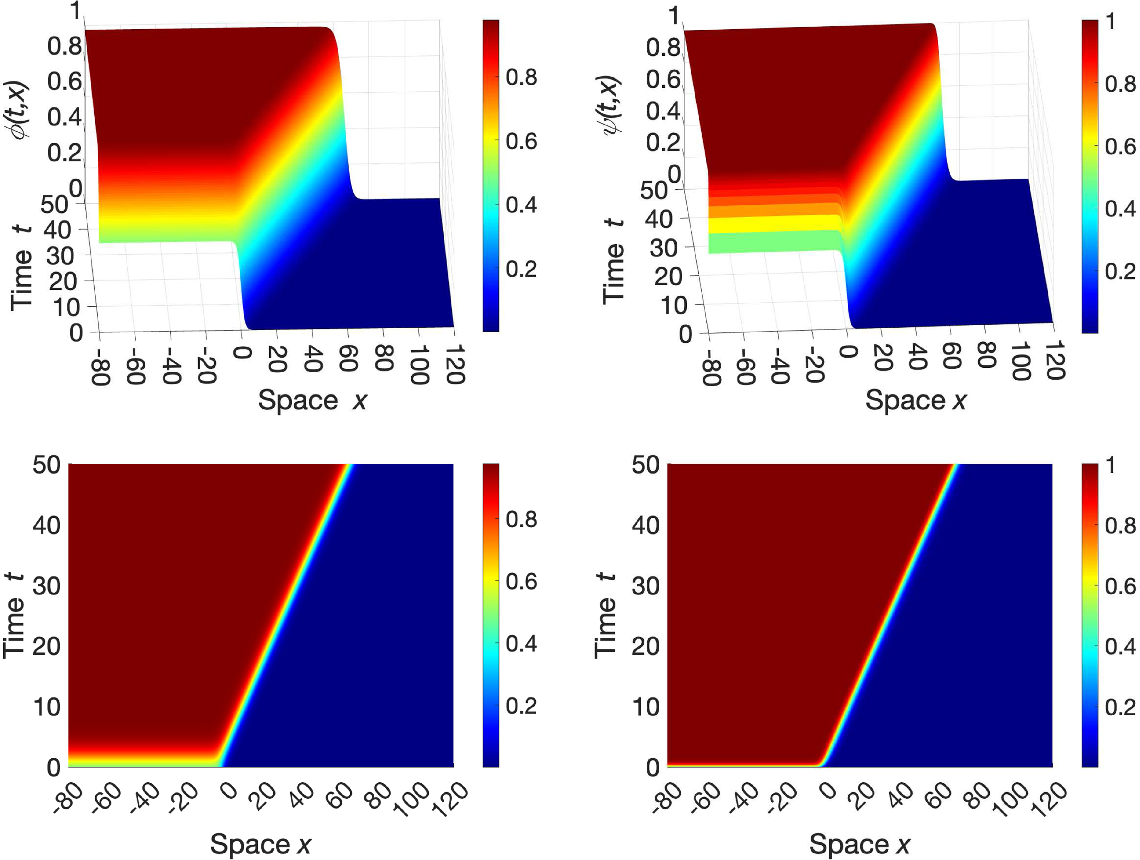
Figure 2. The simulation of $(\phi, \psi )(t,x)$
is carried out based on case H2, with parameter values set as
$(\phi, \psi )(t,x)$
is carried out based on case H2, with parameter values set as $b=5$
and
$b=5$
and $r=0.5$
. The spatiotemporal dynamics of
$r=0.5$
. The spatiotemporal dynamics of $\phi$
and
$\phi$
and $\psi$
are presented in the first row, while the corresponding 2-D plots viewed from the top are shown in the bottom row.
$\psi$
are presented in the first row, while the corresponding 2-D plots viewed from the top are shown in the bottom row.
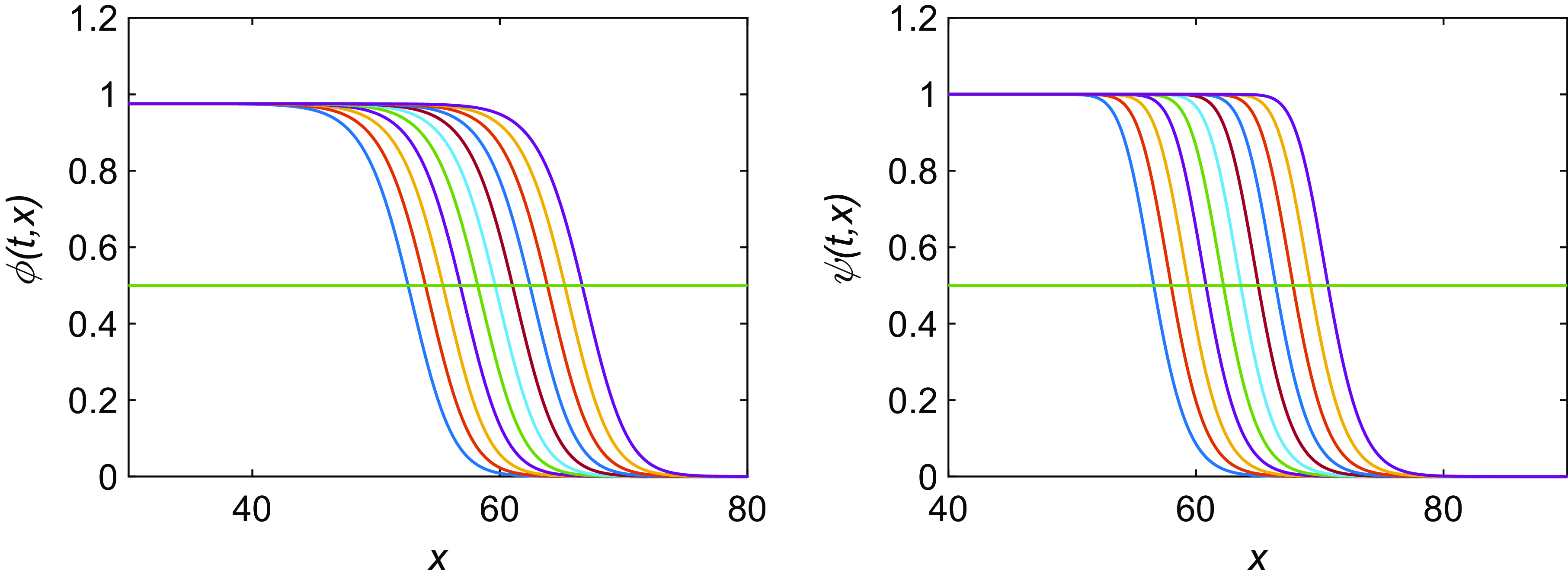
Figure 3. Snapshots of $\phi (t,x)$
and
$\phi (t,x)$
and $\psi (t,x)$
’s movements. The graph on the left represents
$\psi (t,x)$
’s movements. The graph on the left represents $\phi (t,x)$
, while the graph on the right represents
$\phi (t,x)$
, while the graph on the right represents $\psi (t,x)$
. These snapshots correspond to different time values
$\psi (t,x)$
. These snapshots correspond to different time values $t=40,41,42,\ldots 50$
.
$t=40,41,42,\ldots 50$
.
Theorem3.6 shows that the minimal speed $c_{\min }$
has a monotonic relationship with the parameter
$c_{\min }$
has a monotonic relationship with the parameter $b$
. Additionally, this theorem offers a necessary and sufficient criterion for distinguishing between linear and nonlinear selection based on the value of
$b$
. Additionally, this theorem offers a necessary and sufficient criterion for distinguishing between linear and nonlinear selection based on the value of $b$
. Theorem3.10 illustrates that there exists a unique turning point
$b$
. Theorem3.10 illustrates that there exists a unique turning point $r^*$
for speed selection when
$r^*$
for speed selection when $b$
is fixed. The numerical simulation presented in Figure 4 aligns with the findings outlined in Theorems3.6 and 3.10.
$b$
is fixed. The numerical simulation presented in Figure 4 aligns with the findings outlined in Theorems3.6 and 3.10.
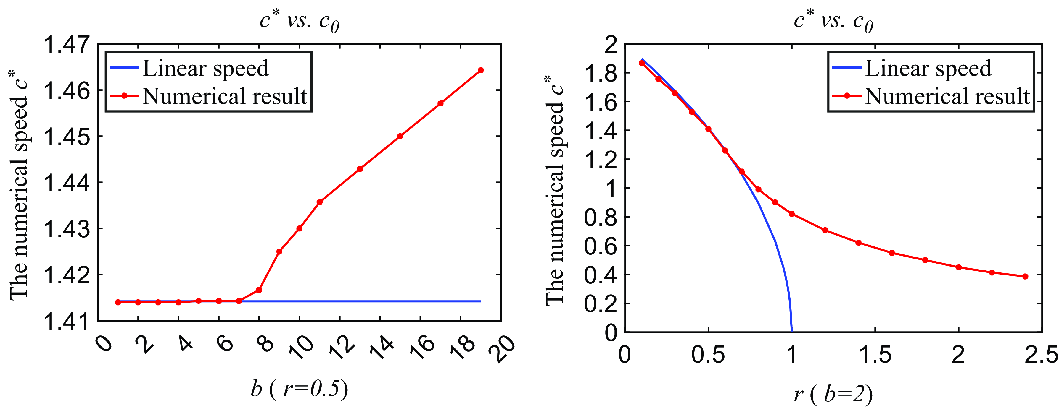
Figure 4. In the left figure, we have $r=0.5$
. It shows the relationship between the numerical moving speed
$r=0.5$
. It shows the relationship between the numerical moving speed $c^*$
and
$c^*$
and $b$
for fixed
$b$
for fixed $r$
. The relationship between
$r$
. The relationship between $c^*$
and
$c^*$
and $r$
, when
$r$
, when $b=2$
, is in the right figure.
$b=2$
, is in the right figure.
For the left picture in Figure 4, we set $r=0.5$
. It is observed that the numerical speed
$r=0.5$
. It is observed that the numerical speed $c^*$
increases monotonically with respect to
$c^*$
increases monotonically with respect to $b$
for a fixed value of
$b$
for a fixed value of $r$
, as shown by the dot-sign (red) curve. The straight (blue) line represents the linear speed, where
$r$
, as shown by the dot-sign (red) curve. The straight (blue) line represents the linear speed, where $c_0=2\sqrt{1-r}\approx 1.4142$
. There exists a turning point
$c_0=2\sqrt{1-r}\approx 1.4142$
. There exists a turning point $b^*$
at which the two curves coincide (
$b^*$
at which the two curves coincide ( $c^*=c_0$
) for
$c^*=c_0$
) for $b\le b^*$
, and
$b\le b^*$
, and $c^*\gt c_0$
for
$c^*\gt c_0$
for $b\gt b^*$
. In our numerical analysis with
$b\gt b^*$
. In our numerical analysis with $r=0.5$
, we find that
$r=0.5$
, we find that $b^*\approx 7$
. In the right figure, we let
$b^*\approx 7$
. In the right figure, we let $b=2$
. The solid (blue) curve is the linear speed
$b=2$
. The solid (blue) curve is the linear speed $c_0=2\sqrt{1-r}$
, and the dot-sign (red) curve is the numerical speed
$c_0=2\sqrt{1-r}$
, and the dot-sign (red) curve is the numerical speed $c^*$
. we can see that there is also a turning point
$c^*$
. we can see that there is also a turning point $r^*$
such that
$r^*$
such that $c^*=c_0$
for
$c^*=c_0$
for $r\le r^*$
, and
$r\le r^*$
, and $c^*\gt c_0$
for
$c^*\gt c_0$
for $r\gt r^*$
. From this figure, we know
$r\gt r^*$
. From this figure, we know $r^*\approx 0.7$
.
$r^*\approx 0.7$
.
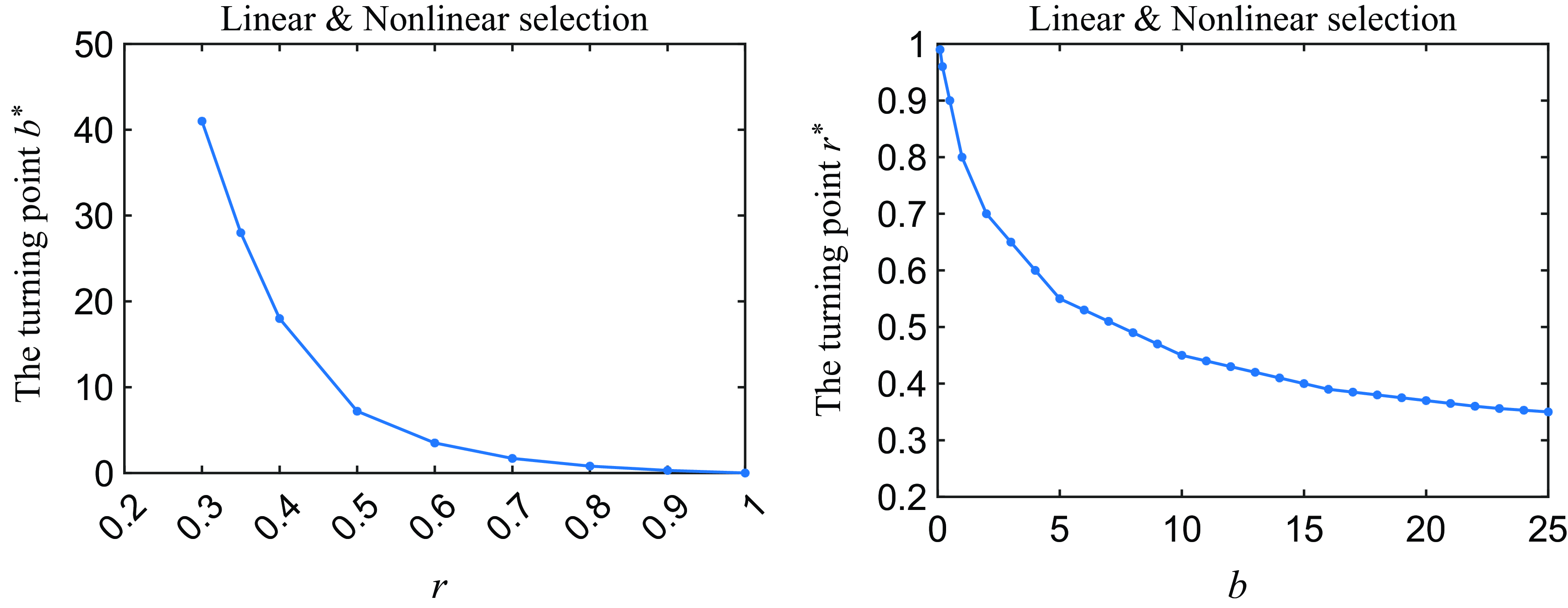
Figure 5. The left diagram illustrates the relationship between $b^*$
and
$b^*$
and $r$
, while the right figure depicts the relation between
$r$
, while the right figure depicts the relation between $r^*$
and
$r^*$
and $b$
.
$b$
.
For the two pictures in Figure 5, if the parameter value is above the curve, the minimal wave speed is nonlinearly selected; otherwise, if the parameter value is below the curve, the minimal wave speed is linearly selected.
5. Conclusion and discussion
In this work, we investigated the existence, uniqueness, speed sign of bistable travelling waves, and the minimal wave speed selection for monostable travelling waves to the Belousov–Zhabotinsky system with spatiotemporal interaction (1.2). As (1.2) exhibits transition dynamics from monostable to bistable for different domains of the system parameter $r$
, we analysed it in two cases, H1(bistable) and H2(monostable). The presence of a non-isolated equilibrium
$r$
, we analysed it in two cases, H1(bistable) and H2(monostable). The presence of a non-isolated equilibrium $e_0$
and a non-local delayed reaction term in the system proposes a challenge for directly applying most existing theories to establish the existence of bistable travelling waves. By developing new ideas such as construction of auxiliary parabolic non-local model, we successfully established the existence and uniqueness of travelling waves under bistable cases H1. It is important to note that the ideas and techniques utilised in this work can be extended and applied to various new systems, particularly those with non-isolated equilibrium points and non-local reaction terms, for which most existing theories do not apply.
$e_0$
and a non-local delayed reaction term in the system proposes a challenge for directly applying most existing theories to establish the existence of bistable travelling waves. By developing new ideas such as construction of auxiliary parabolic non-local model, we successfully established the existence and uniqueness of travelling waves under bistable cases H1. It is important to note that the ideas and techniques utilised in this work can be extended and applied to various new systems, particularly those with non-isolated equilibrium points and non-local reaction terms, for which most existing theories do not apply.
In the monostable case H2, we focused on the speed selection. We established necessary and sufficient conditions for linear and nonlinear selections, as presented in Theorems3.4, 3.6 and 3.10. The existence of transition points $b^*$
(when
$b^*$
(when $r$
is fixed) and
$r$
is fixed) and $r^*$
(when
$r^*$
(when $b$
is fixed) for the selection of the minimal speed was also illustrated in Figure 4. Additionally, we found the decay rate of the travelling wave with the minimal speed as
$b$
is fixed) for the selection of the minimal speed was also illustrated in Figure 4. Additionally, we found the decay rate of the travelling wave with the minimal speed as $z\rightarrow \infty$
in terms of the parameters
$z\rightarrow \infty$
in terms of the parameters $b$
and
$b$
and $r$
, respectively, as shown in Theorems3.9 and 3.11. Moreover, we provided a few explicit estimates for
$r$
, respectively, as shown in Theorems3.9 and 3.11. Moreover, we provided a few explicit estimates for $b^*$
in Theorems3.7 and 3.8.
$b^*$
in Theorems3.7 and 3.8.
Finally, we would like to emphasise and compare the novelty of our findings to previous works. We want to point out that our results can be directly generalised to the localised case ( $(\bar{K}* v)(t, x)=v(t, x)$
) and the local delayed case (
$(\bar{K}* v)(t, x)=v(t, x)$
) and the local delayed case ( $(\bar{K}* v)(t, x)=v(t-h, x)$
) by letting
$(\bar{K}* v)(t, x)=v(t-h, x)$
) by letting $\bar{K}(s,y)=\delta (s)\delta (y)$
and
$\bar{K}(s,y)=\delta (s)\delta (y)$
and $\bar{K}(s,y)=\delta (s-h)\delta (y)$
, respectively. The existence, uniqueness and speed sign of the bistable travelling wave for the localised case and the local delayed case in the system (1.1) can also be derived by Theorems1.1 and 1.2. For the minimal speed of the system (1.1) with
$\bar{K}(s,y)=\delta (s-h)\delta (y)$
, respectively. The existence, uniqueness and speed sign of the bistable travelling wave for the localised case and the local delayed case in the system (1.1) can also be derived by Theorems1.1 and 1.2. For the minimal speed of the system (1.1) with $(\bar{K}* v)(t, x)=v(t, x)$
, Trofimchuk et al. [Reference Trofimchuk, Pinto and Trofimchuk31] gave information of the minimal speed in the monostable case as follows:
$(\bar{K}* v)(t, x)=v(t, x)$
, Trofimchuk et al. [Reference Trofimchuk, Pinto and Trofimchuk31] gave information of the minimal speed in the monostable case as follows:
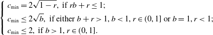 \begin{equation} \left \{\begin{aligned} & c_{\min }= 2\sqrt{1-r}, \ \text{if} \ rb+r\le 1;\\ & c_{\min }\le 2\sqrt{b},\ \text{if either} \ b+r\gt 1,b\lt 1, r\in (0,1] \ \text{or} \ b=1, r\lt 1;\\ &c_{\min }\le 2, \ \text{if} \ b\gt 1, r\in (0,1]. \end{aligned}\right . \end{equation}
We are more concentrated on the speed selection by providing general methods, and our results (Theorems3.4-3.10) can be directly applied to this case when $\bar{K}(s,y)=\delta (s)\delta (y)$
by construction of various upper or lower solutions. In particular, by letting
$\bar{K}(s,y)=\delta (s)\delta (y)$
by construction of various upper or lower solutions. In particular, by letting $\bar{K}(s,y)=\delta (s)\delta (y)$
, the linear selection condition
$\bar{K}(s,y)=\delta (s)\delta (y)$
, the linear selection condition
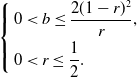 \begin{equation} \left \{\begin{aligned} & 0\lt b\le \frac{2(1-r)^2}{r},\\ & 0\lt r\le \frac{1}{2}. \end{aligned}\right . \end{equation}
in Theorem3.7 is better than $ rb+r\le 1$
in (5.1) when
$ rb+r\le 1$
in (5.1) when $r\le \frac{1}{2}$
, and we also have the nonlinear selection condition
$r\le \frac{1}{2}$
, and we also have the nonlinear selection condition $b\gt \frac{3(1-r)}{2r-1}\ge 0$
which are completely new. Similarly, when
$b\gt \frac{3(1-r)}{2r-1}\ge 0$
which are completely new. Similarly, when $\bar{K}(s,y)=\delta (s-h)\delta (y)$
, we can calculate that the condition (3.31) in Theorem3.7 is better than the linear selection condition
$\bar{K}(s,y)=\delta (s-h)\delta (y)$
, we can calculate that the condition (3.31) in Theorem3.7 is better than the linear selection condition
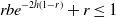 \begin{equation} rbe^{-2h(1-r)}+r\le 1 \end{equation}
in [Reference Trofimchuk, Pinto and Trofimchuk31] of (1.1) with $(\bar{K}* v)(t, x)=v(t-h, x)$
for some domain of
$(\bar{K}* v)(t, x)=v(t-h, x)$
for some domain of $r$
and
$r$
and $h$
. We should mention that we can provide a series of explicit conditions on speed selections by constructing various upper or lower solutions in Theorem3.5. For instance, readers can also apply nonlinear selection condition (Theorem3.8) and necessary and/or sufficient speed selection conditions (Theorems3.4, 3.6 and 3.10) to the model with
$h$
. We should mention that we can provide a series of explicit conditions on speed selections by constructing various upper or lower solutions in Theorem3.5. For instance, readers can also apply nonlinear selection condition (Theorem3.8) and necessary and/or sufficient speed selection conditions (Theorems3.4, 3.6 and 3.10) to the model with $\bar{K}(s,y)=\delta (s-h)\delta (y)$
.
$\bar{K}(s,y)=\delta (s-h)\delta (y)$
.
As we mentioned, the exact or explicit value of the minimal wave speed $c_{\min }$
for the system (1.1) with
$c_{\min }$
for the system (1.1) with $(\bar{K}* v)(t, x)=v(t, x)$
or
$(\bar{K}* v)(t, x)=v(t, x)$
or $(\bar{K}* v)(t, x)=v(t-h, x)$
cannot be worked out [Reference Trofimchuk, Pinto and Trofimchuk31, Reference Trofimchuk, Pinto and Trofimchuk32] in the case of nonlinear selection. Our results can provide some new estimates for
$(\bar{K}* v)(t, x)=v(t-h, x)$
cannot be worked out [Reference Trofimchuk, Pinto and Trofimchuk31, Reference Trofimchuk, Pinto and Trofimchuk32] in the case of nonlinear selection. Our results can provide some new estimates for $c_{\min }$
, whether the system (1.1) is in the localised case or in the local delayed case or in the non-local delayed case.
$c_{\min }$
, whether the system (1.1) is in the localised case or in the local delayed case or in the non-local delayed case.
Financial support
The work was supported by the NSERC discovery grant (RGPIN03842-2021).
Competing interests
We declare none.


 Open access