


1 Introduction
Let $(M,g)$
be a smooth, compact Riemannian manifold with no boundary, unit mass, and let
$(M,g)$
be a smooth, compact Riemannian manifold with no boundary, unit mass, and let $\Delta _g$
denote the Laplace–Beltrami operator. Also, let
$\Delta _g$
denote the Laplace–Beltrami operator. Also, let $\{ \phi _{\lambda } \}$
be an orthonormal basis of eigenfunctions of
$\{ \phi _{\lambda } \}$
be an orthonormal basis of eigenfunctions of $\Delta _g$
with eigenvalues
$\Delta _g$
with eigenvalues $0 \le \lambda _1 \le \lambda _2 \le \ldots $
. For an observable
$0 \le \lambda _1 \le \lambda _2 \le \ldots $
. For an observable $f \in C^{\infty }({\mathbb S}^* M)$
, where
$f \in C^{\infty }({\mathbb S}^* M)$
, where ${\mathbb S}^* M$
denotes the unit cotangent bundle of M, let
${\mathbb S}^* M$
denotes the unit cotangent bundle of M, let $\operatorname {Op}(f)$
denote its quantization, defined as a pseudo-differential operator (cf. [Reference Dimassi and Sjöstrand9] for details.) A central problem in quantum chaos (cf. [Reference Zelditch52, Problem 3.1]) is to understand the set of possible quantum limits (sometimes called semiclassical measures) describing the distribution of mass of the eigenfunctions
$\operatorname {Op}(f)$
denote its quantization, defined as a pseudo-differential operator (cf. [Reference Dimassi and Sjöstrand9] for details.) A central problem in quantum chaos (cf. [Reference Zelditch52, Problem 3.1]) is to understand the set of possible quantum limits (sometimes called semiclassical measures) describing the distribution of mass of the eigenfunctions $\{ \phi _{\lambda } \}$
within
$\{ \phi _{\lambda } \}$
within ${\mathbb S}^* M$
, in the limit as the eigenvalue
${\mathbb S}^* M$
, in the limit as the eigenvalue $\lambda $
tends to infinity. A cornerstone result in this direction is the quantum ergodicity theorem of Shnirelman [Reference Šnirel'man45], Colin de Verdiére [Reference Colin de Verdière8] and Zelditch [Reference Zelditch51] which states that if the geodesic flow on M is ergodic there exists a density one subsequence of eigenfunctions
$\lambda $
tends to infinity. A cornerstone result in this direction is the quantum ergodicity theorem of Shnirelman [Reference Šnirel'man45], Colin de Verdiére [Reference Colin de Verdière8] and Zelditch [Reference Zelditch51] which states that if the geodesic flow on M is ergodic there exists a density one subsequence of eigenfunctions $\{ \phi _{\lambda _j}\}$
such that
$\{ \phi _{\lambda _j}\}$
such that
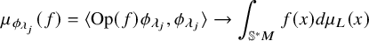 $$\begin{align*}\mu_{\phi_{\lambda_{j}}}(f) =\langle \operatorname{Op}(f) \phi_{\lambda_j}, \phi_{\lambda_j} \rangle \rightarrow \int_{{\mathbb S}^* M} f(x) d\mu_{L}(x)\\[-15pt] \end{align*}$$
as $\lambda _j \rightarrow \infty $
, where
$\lambda _j \rightarrow \infty $
, where $d\mu _{L}$
is the normalized Liouville measure on
$d\mu _{L}$
is the normalized Liouville measure on ${\mathbb S}^* M$
. (Note that any quantum limit, by Egorov’s theorem, is invariant under the classical dynamics.)
${\mathbb S}^* M$
. (Note that any quantum limit, by Egorov’s theorem, is invariant under the classical dynamics.)
While the quantum ergodicity theorem implies that the mass of almost all eigenfunctions equidistributes in ${\mathbb S}^{*} M$
with respect to
${\mathbb S}^{*} M$
with respect to $d\mu _{L}$
, it does not rule out the existence of sparse subsequences along which the mass of the eigenfunctions localizes. Whether or not this happens crucially depends on the geometry of M, cf. Section 1.3.
$d\mu _{L}$
, it does not rule out the existence of sparse subsequences along which the mass of the eigenfunctions localizes. Whether or not this happens crucially depends on the geometry of M, cf. Section 1.3.
In this article, we study quantum limits of ‘point scatterers’ on $M=\mathbb T^2=\mathbb R^2/2\pi \mathbb Z^2$
. These are singular perturbations of the Laplacian on M and were used by Šeba [Reference Šeba40] in order to study the transition between integrability and chaos in quantum systems. The perturbation is quite weak and has essentially no effect on the classical dynamics, yet the quantum dynamics ‘feels’ the effect of the scatterer, and an analog of the quantum ergodicity theorem is known to hold [Reference Rudnick and Ueberschär38, Reference Kurlberg and Ueberschär27] (namely, equidistribution holds for a full density subset of the ‘new’ eigenfunctions), even though classical ergodicity does not hold.
$M=\mathbb T^2=\mathbb R^2/2\pi \mathbb Z^2$
. These are singular perturbations of the Laplacian on M and were used by Šeba [Reference Šeba40] in order to study the transition between integrability and chaos in quantum systems. The perturbation is quite weak and has essentially no effect on the classical dynamics, yet the quantum dynamics ‘feels’ the effect of the scatterer, and an analog of the quantum ergodicity theorem is known to hold [Reference Rudnick and Ueberschär38, Reference Kurlberg and Ueberschär27] (namely, equidistribution holds for a full density subset of the ‘new’ eigenfunctions), even though classical ergodicity does not hold.
The model also exhibits scarring along sparse subsequences of the new eigenfunctions [Reference Kurlberg and Rosenzweig25]. In particular, there exist quantum limits whose momentum push-forwards, which can be viewed as probability measures on the unit circle, are of the form $c \mu _{\text {sing}} + (1-c) \mu _{\text {uniform}}$
, for some
$c \mu _{\text {sing}} + (1-c) \mu _{\text {uniform}}$
, for some $c \in [1/2,1]$
. Here, both
$c \in [1/2,1]$
. Here, both $\mu _{\text {uniform}}$
and
$\mu _{\text {uniform}}$
and $\mu _{\text {sing}}$
are normalized to have mass one, and
$\mu _{\text {sing}}$
are normalized to have mass one, and $\mu _{\text {sing}}$
can be taken to be a sum of delta measures giving equal mass to the four points
$\mu _{\text {sing}}$
can be taken to be a sum of delta measures giving equal mass to the four points $\pm (1,0), \pm (0,1)$
. We note that
$\pm (1,0), \pm (0,1)$
. We note that $\mu _{\text {uniform}}$
is the push-forward of the Liouville measure and hence maximally delocalized, whereas
$\mu _{\text {uniform}}$
is the push-forward of the Liouville measure and hence maximally delocalized, whereas $\mu _{\text {sing}}$
is maximally localized since any quantum limits in this setting must be invariant under a certain eight fold symmetry (cf. equation (1.7)).
$\mu _{\text {sing}}$
is maximally localized since any quantum limits in this setting must be invariant under a certain eight fold symmetry (cf. equation (1.7)).
Stronger localization, that is, going beyond $c=1/2$
, is interesting given a number of ‘half delocalization’ results for quantum limits for some other (strongly chaotic) systems, namely quantized cat maps and geodesic flows on manifolds with constant negative curvature
$c=1/2$
, is interesting given a number of ‘half delocalization’ results for quantum limits for some other (strongly chaotic) systems, namely quantized cat maps and geodesic flows on manifolds with constant negative curvature $-1$
. In the former case, Faure and Nonnenmacher showed [Reference Faure and Nonnenmacher12] that if a quantum limit
$-1$
. In the former case, Faure and Nonnenmacher showed [Reference Faure and Nonnenmacher12] that if a quantum limit $\nu $
is decomposed as
$\nu $
is decomposed as $\nu = \nu _{\text {pp}} + \nu _{\text {Liouville}} + \nu _{sc}$
, with
$\nu = \nu _{\text {pp}} + \nu _{\text {Liouville}} + \nu _{sc}$
, with $\nu _{\text {pp}}$
denoting the pure point part and
$\nu _{\text {pp}}$
denoting the pure point part and $\nu _{sc}$
denoting the singular continuous part, then
$\nu _{sc}$
denoting the singular continuous part, then $\nu _{\text {Liouville}}({\mathbb T}^2) \ge \nu _{\text {pp}}({\mathbb T}^2)$
, and thus
$\nu _{\text {Liouville}}({\mathbb T}^2) \ge \nu _{\text {pp}}({\mathbb T}^2)$
, and thus $\nu _{\text {pp}}({\mathbb T}^2) \le 1/2$
. (We emphasize that
$\nu _{\text {pp}}({\mathbb T}^2) \le 1/2$
. (We emphasize that ${\mathbb T}^{2}$
is the full phase space in this setting.) In the latter case, it was shown that the Kolmogorov-Sinai (KS) entropy with respect to any measure arising as a quantum limit is at least
${\mathbb T}^{2}$
is the full phase space in this setting.) In the latter case, it was shown that the Kolmogorov-Sinai (KS) entropy with respect to any measure arising as a quantum limit is at least $1/2$
. We remark that for arithmetic point scatterers, the KS entropy is zero with respect to any flow invariant probability measure, in particular for any measure arising as a quantum limit.
$1/2$
. We remark that for arithmetic point scatterers, the KS entropy is zero with respect to any flow invariant probability measure, in particular for any measure arising as a quantum limit.
The aim of this paper is to exhibit essentially maximal localization for a quantum ergodic system, namely arithmetic toral point scatterers. In particular, we construct quantum limits (in momentum) corresponding to $c=1$
in the above decomposition; other interesting examples include singular continuous measures with support, say, on Cantor sets. This can be viewed as a step towards a ‘measure classification’ for quantum limits of quantum ergodic systems.
$c=1$
in the above decomposition; other interesting examples include singular continuous measures with support, say, on Cantor sets. This can be viewed as a step towards a ‘measure classification’ for quantum limits of quantum ergodic systems.
1.1 Description of the model
Let us now describe the basic properties of the point scatterer. This is discussed in further detail in [Reference Rudnick and Ueberschär38, Reference Rudnick and Ueberschär39, Reference Kurlberg and Ueberschär27, Reference Kurlberg and Rosenzweig25, Reference Šeba40, Reference Shigehara42]. To describe the quantum system associated with the point scatterer, consider $ -\Delta |_{D_{x_0}}, $
where
$ -\Delta |_{D_{x_0}}, $
where
 $$\begin{align*}D_{x_0}=\{ f \in L^2(\mathbb T^2) : f(x) =0 \text{ in some neighborhood of } x_0 \}. \end{align*}$$
By von Neumann’s theory of self-adjoint extensions (see Appendix A of [Reference Rudnick and Ueberschär38]) there exists a one parameter family of self-adjoint extension of $-\Delta |_{D_{x_0}}$
parameterized by a phase
$-\Delta |_{D_{x_0}}$
parameterized by a phase $\varphi \in (- \pi , \pi ]$
. Moreover, for
$\varphi \in (- \pi , \pi ]$
. Moreover, for $\varphi \neq \pi $
the eigenvalues of these operators may be divided into two categories. The old eigenvalues which are eigenvalues of
$\varphi \neq \pi $
the eigenvalues of these operators may be divided into two categories. The old eigenvalues which are eigenvalues of $-\Delta $
, with multiplicity decreased by one, along with new eigenvalues which are solutions to the spectral equation
$-\Delta $
, with multiplicity decreased by one, along with new eigenvalues which are solutions to the spectral equation
 $$ \begin{align} \sum_{m \ge 1} r(m) \left( \frac{1}{m-\lambda}-\frac{m}{m^2+1} \right)=\tan(\varphi/2)\sum_{m\ge 1} \frac{r(m)}{m^2+1}, \end{align} $$
where
 $$\begin{align*}r(m)=\# \{ (a,b) \in \mathbb Z^2 : a^2+b^2=m\}. \end{align*}$$
We will refer to the case when $\varphi $
is fixed as
$\varphi $
is fixed as $\lambda \rightarrow \infty $
the weak coupling quantization. In this regime work of Shigehara [Reference Shigehara42] suggests that the level spacing of the eigenvalues should have Poisson spacing statistics, and this is supported by work of Rudnick and Ueberschär [Reference Rudnick and Ueberschär39] along with Freiberg, Kurlberg and Rosenzweig [Reference Freiberg, Kurlberg and Rosenzweig14]. In the hope of exhibiting wave chaos, Shigehara proposes the following strong coupling quantization
$\lambda \rightarrow \infty $
the weak coupling quantization. In this regime work of Shigehara [Reference Shigehara42] suggests that the level spacing of the eigenvalues should have Poisson spacing statistics, and this is supported by work of Rudnick and Ueberschär [Reference Rudnick and Ueberschär39] along with Freiberg, Kurlberg and Rosenzweig [Reference Freiberg, Kurlberg and Rosenzweig14]. In the hope of exhibiting wave chaos, Shigehara proposes the following strong coupling quantization
 $$ \begin{align} \sum_{|m-\lambda|\le \lambda^{1/2}} r(m) \left( \frac{1}{m-\lambda}-\frac{m}{m^2+1} \right)=\frac{1}{\alpha}, \end{align} $$
where $\alpha \in \mathbb R$
is called the physical coupling constant and reflects the strength of the scatterer. The strong coupling quantization restricts the spectral equation to the physically relevant energy levels. Notably, this forces a renormalization of equation (1.1)
$\alpha \in \mathbb R$
is called the physical coupling constant and reflects the strength of the scatterer. The strong coupling quantization restricts the spectral equation to the physically relevant energy levels. Notably, this forces a renormalization of equation (1.1)
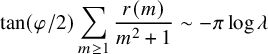 $$\begin{align*}\tan(\varphi/2)\sum_{m \ge 1} \frac{r(m)}{m^2+1} \sim -\pi \log \lambda \end{align*}$$
so that $\varphi $
depends on
$\varphi $
depends on $\lambda $
in this case (see [Reference Ueberschär48] equation (3.14)). We note that the weak coupling quantization corresponds to a fixed self-adjoint extension, whereas the strong coupling quantization can be viewed as an energy-dependent, albeit very slowly varying, family of self-adjoint extensions.
$\lambda $
in this case (see [Reference Ueberschär48] equation (3.14)). We note that the weak coupling quantization corresponds to a fixed self-adjoint extension, whereas the strong coupling quantization can be viewed as an energy-dependent, albeit very slowly varying, family of self-adjoint extensions.
From the spectral equation, it follows that new eigenvalues interlace with integers which are representable as the sum of two integer squares. We denote these eigenvalues as follows:
 $$\begin{align*}0< \lambda_0 < 1 < \lambda_1 < 2 < \lambda_2 <4 < \lambda_4 < 5< \lambda_5 < \cdots \end{align*}$$
and write $\Lambda _{new}$
for the set of all such eigenvalues. Also, given
$\Lambda _{new}$
for the set of all such eigenvalues. Also, given $n=a^2+b^2$
, let
$n=a^2+b^2$
, let $n^+$
denote the smallest integer greater than n which is also a sum of two squares. Let
$n^+$
denote the smallest integer greater than n which is also a sum of two squares. Let
 $$ \begin{align} {s_n}=\lambda_n-n>0 \end{align} $$
denote the distance between $\lambda _n$
and the nearest old eigenvalue n to the left. In addition, given
$\lambda _n$
and the nearest old eigenvalue n to the left. In addition, given $\lambda \in \Lambda _{new}$
the associated Green’s function is given by
$\lambda \in \Lambda _{new}$
the associated Green’s function is given by
 $$ \begin{align} G_{\lambda}(x)=-\frac{1}{4 \pi^2} \sum_{ \xi \in \mathbb Z^2} \frac{ \exp(-i \xi \cdot x_0)}{|\xi|^2- \lambda} e^{i \xi \cdot x}, \qquad g_{\lambda}(x)=\frac{1}{\lVert G_{\lambda} \rVert_2} G_{\lambda}(x) \end{align} $$
(see equation (5.2) of [Reference Rudnick and Ueberschär38]). Also, note that the new eigenvalues interlace between the old eigenvalues; hence, $G_{\lambda }$
is well defined for
$G_{\lambda }$
is well defined for $\lambda \in \Lambda _{new}$
. Since the torus is homogeneous, we may without loss of generality assume that
$\lambda \in \Lambda _{new}$
. Since the torus is homogeneous, we may without loss of generality assume that $x_{0}=0$
. Our main focus will be the behavior of the matrix coefficients
$x_{0}=0$
. Our main focus will be the behavior of the matrix coefficients $ \{\langle \operatorname {Op}(f) g_{\lambda }, g_{\lambda } \rangle \}_{\lambda \in \Lambda _{new}}$
as f ranges over the set of pure momentum observables (i.e.,
$ \{\langle \operatorname {Op}(f) g_{\lambda }, g_{\lambda } \rangle \}_{\lambda \in \Lambda _{new}}$
as f ranges over the set of pure momentum observables (i.e., $f \in C^{\infty } (S^1) \subset C^{\infty }({\mathbb S}^{*}(\mathbb T^2))$
; for such f the matrix coefficients are explicitly given by (cf. equation (5.3))
$f \in C^{\infty } (S^1) \subset C^{\infty }({\mathbb S}^{*}(\mathbb T^2))$
; for such f the matrix coefficients are explicitly given by (cf. equation (5.3))
 $$ \begin{align} \langle \operatorname{Op}(f) g_{\lambda}, g_{\lambda} \rangle = \frac{1}{\sum_{n \ge 0} \frac{r(n)}{(n-\lambda)^2}} \left( \frac{f(1)}{\lambda^{2}} + \sum_{ n> 0 }\frac{1}{(n-\lambda)^2} \sum_{ a^2+b^2=n} f\left(\frac{a+ib}{|a+ib|} \right) \right). \end{align} $$
1.2 Results
Our first main result shows that along a zero density, yet relatively large, subsequence of new eigenvalues $\{\lambda _j\}$
the mass of
$\{\lambda _j\}$
the mass of $g_{\lambda _j}$
, in momentum space, localizes on measures arising from
$g_{\lambda _j}$
, in momentum space, localizes on measures arising from ${\mathbb Z}^2$
-lattice points on circles (after projecting them to the unit circle). To describe these measures in more detail, consider an integer
${\mathbb Z}^2$
-lattice points on circles (after projecting them to the unit circle). To describe these measures in more detail, consider an integer $n=a^2+b^2$
, with
$n=a^2+b^2$
, with $a,b\in {\mathbb Z}$
, and the following probability measure on the unit circle
$a,b\in {\mathbb Z}$
, and the following probability measure on the unit circle $S^1 \subset {\mathbb C}$
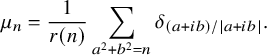 $$\begin{align*}\mu_n =\frac{1}{r(n)} \sum_{a^2+b^2=n} \delta_{(a+ib)/|a+ib|}. \end{align*}$$
We remark that $\mu _n$
can be viewed as the matrix coefficient of the ‘flat’ (old) Laplace eigenfunction
$\mu _n$
can be viewed as the matrix coefficient of the ‘flat’ (old) Laplace eigenfunction $ \psi _n(x) = \frac {1}{2 \pi \sqrt {r(n)}} \sum _{\xi \in {\mathbb Z}^2 : |\xi |^{2} = n} e^{ -i \xi \cdot x }, $
in the sense that, for f a pure momentum observable, we have
$ \psi _n(x) = \frac {1}{2 \pi \sqrt {r(n)}} \sum _{\xi \in {\mathbb Z}^2 : |\xi |^{2} = n} e^{ -i \xi \cdot x }, $
in the sense that, for f a pure momentum observable, we have
 $$ \begin{align} \langle \operatorname{Op}(f) \psi_{n}, \psi_{n}\rangle = \sum_{ a^2+b^2=n} f\left(\frac{a+ib}{|a+ib|} \right) = \mu_n(f).\\[-9pt]\nonumber \end{align} $$
Following Kurlberg and Wigman [Reference Kurlberg and Wigman29], we call a measure $\mu _{\infty }$
attainable if it is a weak limit point of the set
$\mu _{\infty }$
attainable if it is a weak limit point of the set $\{ \mu _n \}_{n=a^2+b^2}$
. Any such measure is invariant under rotation by
$\{ \mu _n \}_{n=a^2+b^2}$
. Any such measure is invariant under rotation by $\pi /2$
, as well as under reflection in the x-axis; for convenience let
$\pi /2$
, as well as under reflection in the x-axis; for convenience let
 $$ \begin{align} \text{Sym}_{8} := \left\{ \left\langle \begin{pmatrix} 0 & -1 \\ 1 & 0 \end{pmatrix}, \begin{pmatrix} -1 & 0 \\ 0 & 1 \end{pmatrix} \right\rangle \right\} \subset GL_{2}({\mathbb Z})\\[-9pt]\nonumber \end{align} $$
denote the group generated by these transformations.
Theorem 1.1. Let $m_0=a^2+b^2 \in \mathbb N$
be odd.Footnote
1
In each of the weak and strong coupling quantizations, there exists a subset of eigenvalues
$m_0=a^2+b^2 \in \mathbb N$
be odd.Footnote
1
In each of the weak and strong coupling quantizations, there exists a subset of eigenvalues ${\mathcal E}_{m_0} \subset \Lambda _{new}$
with
${\mathcal E}_{m_0} \subset \Lambda _{new}$
with
 $$\begin{align*}\frac{ \# \{ \lambda \le X : \lambda \in {\mathcal E}_{m_0} \}}{\# \{ \lambda \le X : \lambda \in \Lambda_{\text{new}} \} } \gg \frac{1 }{(\log X)^{1+o(1)}}\\[-9pt] \end{align*}$$
such that for any pure momentum observable $f \in C^{\infty } (S^1) \subset C^{\infty }(\mathbb S^{*}(\mathbb T^2))$
 $$\begin{align*}\langle \operatorname{Op}(f) g_{\lambda}, g_{\lambda} \rangle \xrightarrow{ \substack{\lambda \rightarrow \infty \\ \lambda \in {\mathcal E}_{m_0}}} \frac{1}{r(m_0)} \sum_{a^2+b^2=m_0} f\left(\frac{a+ib}{|a+ib|} \right).\\[-9pt] \end{align*}$$
The key idea of the proof is to show that some new eigenvalues $\lambda $
lie very close to certain old eigenvalues n, and this implies that
$\lambda $
lie very close to certain old eigenvalues n, and this implies that $g_{\lambda }$
is very well approximated by the flat eigenfunction
$g_{\lambda }$
is very well approximated by the flat eigenfunction $\psi _{n}$
(cf. equations (1.5) and (1.6)), and consequently, in momentum space, the mass of
$\psi _{n}$
(cf. equations (1.5) and (1.6)), and consequently, in momentum space, the mass of $g_{\lambda }$
completely localizes on the measure
$g_{\lambda }$
completely localizes on the measure $ \mu _{m_0}$
. Further, for any attainable measure
$ \mu _{m_0}$
. Further, for any attainable measure $\mu _{\infty }$
there exists
$\mu _{\infty }$
there exists $\{m_{0, \ell } \}_{\ell }$
such that
$\{m_{0, \ell } \}_{\ell }$
such that $\mu _{m_{0},\ell }$
weakly converges to
$\mu _{m_{0},\ell }$
weakly converges to $\mu _{\infty }$
, and this implies the following corollary.
$\mu _{\infty }$
, and this implies the following corollary.
Corollary 1.1. Let $\mu _{\infty }$
be an attainable measure. Then there exists
$\mu _{\infty }$
be an attainable measure. Then there exists $\{\lambda _j\}_{j} \subset \Lambda _{\text {new}}$
such that for any pure momentum observable
$\{\lambda _j\}_{j} \subset \Lambda _{\text {new}}$
such that for any pure momentum observable $f \in C^{\infty }(S^1) $
 $$\begin{align*}\langle \operatorname{Op}(f) g_{\lambda_j}, g_{\lambda_j} \rangle \xrightarrow{j \rightarrow \infty} \int_{S^1} f d\mu_{\infty}.\\[-9pt] \end{align*}$$
We note that the set of attainable measures is much smaller than the set of probability measures on $S^{1}$
that are
$S^{1}$
that are $\text {Sym}_{8}$
-invariant, in particular the set of attainable measures is not convex (cf. [Reference Kurlberg and Wigman29, Section 3.2].) In our next result, we show that in the strong coupling quantization there is a subsequence of new eigenvalues along which the entire mass of
$\text {Sym}_{8}$
-invariant, in particular the set of attainable measures is not convex (cf. [Reference Kurlberg and Wigman29, Section 3.2].) In our next result, we show that in the strong coupling quantization there is a subsequence of new eigenvalues along which the entire mass of $g_{\lambda }$
localizes on a certain convex combination of two measures arising from lattice points on the circle. In particular, the set of quantum limits, in momentum space, is strictly richer than the set of attainable measures.
$g_{\lambda }$
localizes on a certain convex combination of two measures arising from lattice points on the circle. In particular, the set of quantum limits, in momentum space, is strictly richer than the set of attainable measures.
Theorem 1.2. Let $m_0,m_1$
be odd integers which are each representable as a sum of two squares. Then in the strong coupling quantization there exists a subsequence of eigenvalues
$m_0,m_1$
be odd integers which are each representable as a sum of two squares. Then in the strong coupling quantization there exists a subsequence of eigenvalues $ {\mathcal E}_{m_0,m_1} \subset \Lambda _{\text {new}}$
such that for each
$ {\mathcal E}_{m_0,m_1} \subset \Lambda _{\text {new}}$
such that for each $\lambda \in {\mathcal E}_{m_0,m_1}$
there is an integer
$\lambda \in {\mathcal E}_{m_0,m_1}$
there is an integer $\ell _{\lambda }$
with
$\ell _{\lambda }$
with $r(\ell _{\lambda }) \neq 0$
and
$r(\ell _{\lambda }) \neq 0$
and $r(\ell _{\lambda }) \ll 1$
such that for pure momentum observables
$r(\ell _{\lambda }) \ll 1$
such that for pure momentum observables $f \in C^{\infty }(S^1)$
 $$ \begin{align} \begin{aligned} \langle \operatorname{Op}(f) g_{\lambda}, g_{\lambda} \rangle =\,& c_{\lambda} \cdot \frac{1}{r(m_0)} \sum_{a^2+b^2=m_0} f\left( \frac{a+ib}{|a+ib|}\right) \\ & + (1-c_{\lambda}) \cdot \frac{1}{r(m_1\ell_{\lambda})} \sum_{a^2+b^2=m_1 \ell_{\lambda}} f\left( \frac{a+ib}{|a+ib|}\right)+O\left(\frac{1}{(\log \log \lambda)^{1/11}} \right), \end{aligned} \end{align} $$
where
 $$\begin{align*}c_{\lambda}=\frac{1}{1+r(m_0)/r(m_1\ell_{\lambda})}. \end{align*}$$
Additionally,
 $$\begin{align*}\frac{ \# \{ \lambda \le X : \lambda \in {\mathcal E}_{m_0,m_1} \}}{\# \{ \lambda \le X : \lambda \in \Lambda_{\text{new}} \} } \gg \frac{1 }{(\log X)^{2+o(1)}}. \end{align*}$$
Note that, since $\sum _{p|\ell _{\lambda }} 1 \ll 1$
, the measure
$\sum _{p|\ell _{\lambda }} 1 \ll 1$
, the measure $\mu _{m_{1} \ell _{\lambda }}$
can be viewed as a fairly small perturbation of
$\mu _{m_{1} \ell _{\lambda }}$
can be viewed as a fairly small perturbation of $\mu _{m_{1}}$
.
$\mu _{m_{1}}$
.
Remark 1. By removing a further ‘thin’ set of eigenvalues (with spectral counting function of size $O(x^{1-\epsilon })$
for
$O(x^{1-\epsilon })$
for $\epsilon>0$
, we can construct quantum limits that are flat in position (for details, cf. [Reference Kurlberg and Rosenzweig25, Remark 4]), in addition to the momentum push-forward properties given in Theorems 1.1 and 1.2. In particular, taking say
$\epsilon>0$
, we can construct quantum limits that are flat in position (for details, cf. [Reference Kurlberg and Rosenzweig25, Remark 4]), in addition to the momentum push-forward properties given in Theorems 1.1 and 1.2. In particular, taking say $m_{0}=9$
in Theorem 1.1 and noting that
$m_{0}=9$
in Theorem 1.1 and noting that $|z|^{2} = 9$
for
$|z|^{2} = 9$
for $z \in {\mathbb Z}[i]$
has the four solutions
$z \in {\mathbb Z}[i]$
has the four solutions $\pm 3, \pm 3i$
, this then yields quantum limits that are completely localized on the superposition of two Lagrangian states – essentially two plane waves, one in the horizontal and one in the vertical direction. This phenomenon is sometimes called superscarring (cf. [Reference Bogomolny and Schmit6, Reference Kurlberg and Rosenzweig25]).
$\pm 3, \pm 3i$
, this then yields quantum limits that are completely localized on the superposition of two Lagrangian states – essentially two plane waves, one in the horizontal and one in the vertical direction. This phenomenon is sometimes called superscarring (cf. [Reference Bogomolny and Schmit6, Reference Kurlberg and Rosenzweig25]).
Further, assuming a plausible conjecture on the distribution of the prime numbers, we show that given $m_0,m_1$
as in Theorem 1.2 the quantum limit of
$m_0,m_1$
as in Theorem 1.2 the quantum limit of $\langle \operatorname {Op}(f) g_{\lambda }, g_{\lambda } \rangle $
can be made to be any given convex combination of
$\langle \operatorname {Op}(f) g_{\lambda }, g_{\lambda } \rangle $
can be made to be any given convex combination of $\mu _{m_0}$
and
$\mu _{m_0}$
and $\mu _{m_1}$
. The conjecture on the distribution of primes concerns obtaining a lower bound on the number solutions
$\mu _{m_1}$
. The conjecture on the distribution of primes concerns obtaining a lower bound on the number solutions $(u,v)$
in almost primes to the Diophantine equation
$(u,v)$
in almost primes to the Diophantine equation
 $$\begin{align*}aX-bY=4, \end{align*}$$
where $v=p_1p_2$
,
$v=p_1p_2$
, $u=p_3$
with
$u=p_3$
with $p_j$
a prime satisfying
$p_j$
a prime satisfying $p_j=a_j^2+b_j^2$
and
$p_j=a_j^2+b_j^2$
and $b_j=o(a_j)$
for
$b_j=o(a_j)$
for $j=1,2,3$
. The precise formulation of this conjecture, which we call Hypothesis 1, is given in Section 5.5.
$j=1,2,3$
. The precise formulation of this conjecture, which we call Hypothesis 1, is given in Section 5.5.
Theorem 1.3. Assume Hypothesis 1. Let $\mu _{\infty _0}, \mu _{\infty _1}$
be attainable measures and
$\mu _{\infty _0}, \mu _{\infty _1}$
be attainable measures and $0\le c \le 1$
. Then in the strong coupling quantization there exists
$0\le c \le 1$
. Then in the strong coupling quantization there exists $\{ \lambda _j \}_{j} \subset \Lambda _{new}$
such that for any
$\{ \lambda _j \}_{j} \subset \Lambda _{new}$
such that for any $f \in C^{\infty }(S^1)$
 $$\begin{align*}\langle \operatorname{Op}(f) g_{\lambda_j}, g_{\lambda_j} \rangle \xrightarrow{ j \rightarrow \infty} c\int_{S^1} f d\mu_{\infty_0} +(1-c) \int_{S^1} f d\mu_{\infty_1}. \end{align*}$$
Further, assuming a variation of the prime k-tuple conjecture that also allows for prescribing Gaussian angles, we can show (cf. Appendix C) that all $\text {Sym}_{8}$
-invariant probability measures on
$\text {Sym}_{8}$
-invariant probability measures on $S^{1}$
arise as quantum limits in momentum space.
$S^{1}$
arise as quantum limits in momentum space.
1.3 Discussion
For integrable systems it is often straightforward to construct nonuniform quantum limits, for example, ‘whispering gallery modes’ for the geodesic flow in the unit ball, and for linear flows on ${\mathbb T}^2$
, Lagrangian states with maximal localization (i.e., a single plane wave) are easily constructed. We note that strong localization in position for quantum limits on
${\mathbb T}^2$
, Lagrangian states with maximal localization (i.e., a single plane wave) are easily constructed. We note that strong localization in position for quantum limits on ${\mathbb T}^2$
was ruled out by Jakobson [Reference Jakobson20] – in position, any quantum limit is given by trigonometric polynomials whose frequencies lie on at most two circles (hence absolutely continuous with respect to Lebesgue measure.) Further, for the sphere, Jakobson and Zelditch in fact obtained a full classification – any flow invariant measure on
${\mathbb T}^2$
was ruled out by Jakobson [Reference Jakobson20] – in position, any quantum limit is given by trigonometric polynomials whose frequencies lie on at most two circles (hence absolutely continuous with respect to Lebesgue measure.) Further, for the sphere, Jakobson and Zelditch in fact obtained a full classification – any flow invariant measure on $S^{*}(S^{2})$
is a quantum limit [Reference Jakobson and Zelditch21].
$S^{*}(S^{2})$
is a quantum limit [Reference Jakobson and Zelditch21].
The quantum ergodicity theorem holds in great generality as long as the key assumption of ergodic classical dynamics holds, but the existence of exceptional subsequence of nonuniform quantum limits (‘scarring’) is subtle. For classical systems given by the geodesic flow on compact negatively curved manifolds, the celebrated quantum unique ergodicity (QUE) conjecture [Reference Rudnick and Sarnak37] by Rudnick and Sarnak asserts that the only possible quantum limit is the Liouville measure. Known results for QUE include Lindenstrauss’ breakthrough [Reference Lindenstrauss30] for Hecke eigenfunctions on arithmetic modular surfaces, together with Soundararajan ruling out ‘escape of mass’ in the noncompact case [Reference Soundararajan46]. On the other hand, for a generic Bunimovich stadium (with strongly chaotic classical dynamics), Hassell [Reference Hassell and Hillairet16] has shown that there exists a subsequence of exceptional eigenstates where the mass localizes on sets of bouncing ball trajectories.
For quantized cat maps, again for Hecke eigenfunctions, QUE is known to hold [Reference Kurlberg and Rudnick26]. However, unlike for arithmetic modular surfaces, where Hecke desymmetrization is believed to be unnecessary, it is essential for quantum cat maps. Namely, Faure, Nonnenmacher and de Bièvre [Reference Faure, Nonnenmacher and De Bièvre13] constructed, in the presence of extreme spectral multiplicities and no Hecke desymmetrization, quantum limits of the form $\nu = \frac {1}{2} \nu _{\text {pp}} + \frac {1}{2} \nu _{\text {Liouville}}$
; in [Reference Faure and Nonnenmacher12], this was shown to be sharp in the sense that the Liouville component always carries at least as much mass as the pure point one. (We note that, on assuming very weak bounds on spectral multiplicities, Bourgain showed [Reference Bourgain7] that scarring does not occur.) For higher-dimensional analogs of quantum cat maps, Kelmer has for certain maps shown [Reference Kelmer23] ‘super scarring’, even after Hecke desymmetrization, on invariant rational isotropic subspaces. Further, these type of scars persist on adding certain perturbations that destroy the spectral multiplicities [Reference Kelmer24]. Other models where scarring is known to exist include toral point scatterers with irrational aspect ratios [Reference Kurlberg and Ueberschär28, Reference Keating, Marklof and Winn22, Reference Berkolaiko, Keating and Winn3] and quantum star graphs [Reference Berkolaiko, Keating and Winn4], though neither model is quantum ergodic [Reference Kurlberg and Ueberschär28, Reference Berkolaiko, Keating and Winn4].
$\nu = \frac {1}{2} \nu _{\text {pp}} + \frac {1}{2} \nu _{\text {Liouville}}$
; in [Reference Faure and Nonnenmacher12], this was shown to be sharp in the sense that the Liouville component always carries at least as much mass as the pure point one. (We note that, on assuming very weak bounds on spectral multiplicities, Bourgain showed [Reference Bourgain7] that scarring does not occur.) For higher-dimensional analogs of quantum cat maps, Kelmer has for certain maps shown [Reference Kelmer23] ‘super scarring’, even after Hecke desymmetrization, on invariant rational isotropic subspaces. Further, these type of scars persist on adding certain perturbations that destroy the spectral multiplicities [Reference Kelmer24]. Other models where scarring is known to exist include toral point scatterers with irrational aspect ratios [Reference Kurlberg and Ueberschär28, Reference Keating, Marklof and Winn22, Reference Berkolaiko, Keating and Winn3] and quantum star graphs [Reference Berkolaiko, Keating and Winn4], though neither model is quantum ergodic [Reference Kurlberg and Ueberschär28, Reference Berkolaiko, Keating and Winn4].
Classifying the set of possible quantum limits, in particular for quantum ergodic settings, is an interesting question. Here, Anantharaman proved very strong results for geodesic flows on negatively curved manifolds [Reference Anantharaman1]: any quantum limit has positive KS entropy with respect to the dynamics of the geodesic flow. In particular, this rules out localization on a finite number of closed geodesics (for compact arithmetic surfaces this was already known due to Rudnick and Sarnak [Reference Rudnick and Sarnak37].) Moreover, in the case of constant negative curvature, Anantharaman and Nonnenmacher showed [Reference Anantharaman and Nonnenmacher2] that the KS-entropy is at least half of the maximum possible. The measure of maximum entropy is given by the Liouville measure, and thus ‘eigenfunctions are at least half delocalized’. Dyatlov and Jin [Reference Dyatlov and Jin10] consequently showed that any quantum limit must have full support in $S^{*}(M)$
, for compact hyperbolic surfaces M with constant negative curvature; together with Nonnenmacher this was recently strengthened [Reference Dyatlov, Jin and Nonnenmacher11] to the include the case of surfaces with variable negative curvature.
$S^{*}(M)$
, for compact hyperbolic surfaces M with constant negative curvature; together with Nonnenmacher this was recently strengthened [Reference Dyatlov, Jin and Nonnenmacher11] to the include the case of surfaces with variable negative curvature.
1.4 Outline of the proofs
Our arguments use the multiplicative structure of the integers to create an imbalance in the spectral equation (1.2) along a zero density, yet relatively large subsequence of new eigenvalues. Through exploiting this imbalance, we control the location of the new eigenvalues in our subsequence and show that they lie close to integers which are sums of two squares (cf. Section 5.3, in particular equation (5.14) for the argument placing full mass at one nearby eigenspace and 5.4, in particular equation (5.18) for placing mass at two nearby eigenspaces.) This greatly amplifies the amount of mass of the corresponding eigenfunctions in momentum space which lies on the terms which correspond to these integers, so much so that the contribution of the remaining terms is negligible in comparison. Consequently, the mass completely localizes on a convex combination of two measures and moreover our construction allows us to completely control the first measure.
In Section 2, we use sieve methods to produce integers $n=p_1p_2$
, where
$n=p_1p_2$
, where $p_j$
,
$p_j$
, $j=1,2$
, is a prime with
$j=1,2$
, is a prime with $p_j=a^2+b^2=(a+ib)(a-ib)$
,
$p_j=a^2+b^2=(a+ib)(a-ib)$
, $0< b \le a$
, with
$0< b \le a$
, with $0\le \arctan (b/a) \le \varepsilon $
, where
$0\le \arctan (b/a) \le \varepsilon $
, where $\varepsilon $
is a small parameter, such that
$\varepsilon $
is a small parameter, such that $Q_0p_1p_2+4$
is also a sum of two squares,
$Q_0p_1p_2+4$
is also a sum of two squares, $Q_1|Q_0p_1p_2+4$
and
$Q_1|Q_0p_1p_2+4$
and $(Q_0p_1p_2+4)/Q_1$
has a bounded number of prime factors, where
$(Q_0p_1p_2+4)/Q_1$
has a bounded number of prime factors, where $Q_0,Q_1$
are large integers whose purpose we will describe later. In particular, we exploit special features of the half-dimensional sieve using an ingenious observation of Huxley and Iwaniec [Reference Huxley and Iwaniec18]. Further, in order to find suitable Gaussian primes in narrow sectors we use a classical result of Hecke together with nontrivial bounds on exponential sums over finite fields to control sums of integral lattice points in narrow sectors with norms lying in arithmetic progressions to large moduli.
$Q_0,Q_1$
are large integers whose purpose we will describe later. In particular, we exploit special features of the half-dimensional sieve using an ingenious observation of Huxley and Iwaniec [Reference Huxley and Iwaniec18]. Further, in order to find suitable Gaussian primes in narrow sectors we use a classical result of Hecke together with nontrivial bounds on exponential sums over finite fields to control sums of integral lattice points in narrow sectors with norms lying in arithmetic progressions to large moduli.
The subsequence of almost primes $\{n_{\ell }\}$
constructed as described above creates the imbalance in the spectral equation (1.2) by boosting the contribution of the terms
$\{n_{\ell }\}$
constructed as described above creates the imbalance in the spectral equation (1.2) by boosting the contribution of the terms $m=Q_0n_{\ell }, Q_0n_{\ell }+4$
, without perturbing the target measure(s). The next step in our argument is to show that this imbalance typically overwhelms the contribution of the remaining terms. To do this, we first show in Section 3 that for all new eigenvalues lying outside a small exceptional set the spectral equation (1.2) can be effectively truncated to integers m with essentially
$m=Q_0n_{\ell }, Q_0n_{\ell }+4$
, without perturbing the target measure(s). The next step in our argument is to show that this imbalance typically overwhelms the contribution of the remaining terms. To do this, we first show in Section 3 that for all new eigenvalues lying outside a small exceptional set the spectral equation (1.2) can be effectively truncated to integers m with essentially $|m-\lambda | \ll (\log \lambda )^{10}$
. This is done by controlling sums of
$|m-\lambda | \ll (\log \lambda )^{10}$
. This is done by controlling sums of $r(n)$
over short intervals and uses a second moment estimate of the Dedekind zeta-function
$r(n)$
over short intervals and uses a second moment estimate of the Dedekind zeta-function $\zeta _{\mathbb Q(i)}$
. In Section 4, we apply this result to new eigenvalues which lie between
$\zeta _{\mathbb Q(i)}$
. In Section 4, we apply this result to new eigenvalues which lie between $Q_0n_{\ell }$
and
$Q_0n_{\ell }$
and $Q_0n_{\ell }+4$
and show that for almost all such new eigenvalues the remaining terms in the spectral sum (i.e.,
$Q_0n_{\ell }+4$
and show that for almost all such new eigenvalues the remaining terms in the spectral sum (i.e., $|m-\lambda | \ll (\log \lambda )^{10}, m \neq Q_0n_{\ell }, Q_0n_{\ell }+4)$
is relatively small, provided that we take
$|m-\lambda | \ll (\log \lambda )^{10}, m \neq Q_0n_{\ell }, Q_0n_{\ell }+4)$
is relatively small, provided that we take $Q_0,Q_1$
sufficiently large thereby boosting the contribution of the closest two terms. This is accomplished by using bounds for sums of multiplicative functions over polynomials due to Henriot [Reference Henriot17]. Crucially, we need good estimates for these sums in terms of the discriminant of the polynomials.
$Q_0,Q_1$
sufficiently large thereby boosting the contribution of the closest two terms. This is accomplished by using bounds for sums of multiplicative functions over polynomials due to Henriot [Reference Henriot17]. Crucially, we need good estimates for these sums in terms of the discriminant of the polynomials.
Finally, to get complete control on the first measure in Theorem 1.2 we choose $Q_0$
so that it is the product of a given fixed integer
$Q_0$
so that it is the product of a given fixed integer $m_0$
and large primes
$m_0$
and large primes $p_{k}=a^2+b^2$
with
$p_{k}=a^2+b^2$
with $0 \le \arctan (b_k/a_k) \le p_k^{-1/10}$
so that the probability measure on
$0 \le \arctan (b_k/a_k) \le p_k^{-1/10}$
so that the probability measure on $S^1$
associated with
$S^1$
associated with $Q_0n_{\ell }$
weakly converges to the measure associated with
$Q_0n_{\ell }$
weakly converges to the measure associated with $m_0$
as
$m_0$
as $\ell \rightarrow \infty $
. This last construction uses work of Ricci [Reference Ricci35] on Gaussian primes in narrow sectors.
$\ell \rightarrow \infty $
. This last construction uses work of Ricci [Reference Ricci35] on Gaussian primes in narrow sectors.
1.5 Notation
We write $f(x) \ll g(x)$
provided that
$f(x) \ll g(x)$
provided that $f(x)=O(g(x))$
. Additionally, if for all x under consideration
$f(x)=O(g(x))$
. Additionally, if for all x under consideration $|f(x)| \ge c g(x)$
we write
$|f(x)| \ge c g(x)$
we write $f(x) \gg g(x)$
. If we have both
$f(x) \gg g(x)$
. If we have both $f(x) \ll g(x)$
and
$f(x) \ll g(x)$
and $f(x) \gg g(x)$
, we write
$f(x) \gg g(x)$
, we write $f(x) \asymp g(x)$
. For some additional notation related to sieves, see Section 2.1.1.
$f(x) \asymp g(x)$
. For some additional notation related to sieves, see Section 2.1.1.
2 Sieve estimates
Let $B_0$
be a sufficiently large integer, define
$B_0$
be a sufficiently large integer, define $\varepsilon = (\log \log x)^{-1/11}$
, and let
$\varepsilon = (\log \log x)^{-1/11}$
, and let
 $$ \begin{align} \begin{aligned} {\mathcal P}_{\varepsilon,x}=\,&\{ p \ge (\log x)^{B_0} : p=a^2+b^2 \, \text{ and } \, 0 < \arctan(b/a) \le \varepsilon \}, \\ {\mathcal P}_{\varepsilon,x}'=\,&\{ p \in {\mathcal P}_{\varepsilon} : p \le x^{1/9}\}. \end{aligned} \end{align} $$
For brevity, we will write ${\mathcal P}_{\varepsilon }$
and
${\mathcal P}_{\varepsilon }$
and ${\mathcal P}_{\varepsilon }'$
for
${\mathcal P}_{\varepsilon }'$
for ${\mathcal P}_{\varepsilon ,x}$
and
${\mathcal P}_{\varepsilon ,x}$
and ${\mathcal P}_{\varepsilon ,x}'$
, respectively. Also, given
${\mathcal P}_{\varepsilon ,x}'$
, respectively. Also, given $f,g : \mathbb N \rightarrow \mathbb C$
we define the Dirichlet convolution of f and g by
$f,g : \mathbb N \rightarrow \mathbb C$
we define the Dirichlet convolution of f and g by
 $$\begin{align*}(f \ast g)(n)=\sum_{ab=n} f(a)g(b). \end{align*}$$
Also, let $Q_0,Q_1 \le (\log x)^{1/10}$
be odd coprime integers whose prime factors are all
$Q_0,Q_1 \le (\log x)^{1/10}$
be odd coprime integers whose prime factors are all $\equiv 1\ \pmod 4$
. Moreover, we assume that
$\equiv 1\ \pmod 4$
. Moreover, we assume that $Q_0=f_0^2 e_0 r_0^{a_0}, Q_1=f_1^2e_1 r_1^{a_1}$
, where
$Q_0=f_0^2 e_0 r_0^{a_0}, Q_1=f_1^2e_1 r_1^{a_1}$
, where $e_0,e_1$
are square-free,
$e_0,e_1$
are square-free, $f_0,f_1 \ll 1$
and
$f_0,f_1 \ll 1$
and $r_0,r_1$
are primes congruent to
$r_0,r_1$
are primes congruent to $1\ \pmod 4$
. Throughout, the arithmetic function
$1\ \pmod 4$
. Throughout, the arithmetic function $b(n)$
is the indicator function of the set of integers which are representable as a sum of two squares. Also, for
$b(n)$
is the indicator function of the set of integers which are representable as a sum of two squares. Also, for ${\mathcal S} \subset \mathbb N$
we define
${\mathcal S} \subset \mathbb N$
we define
 $$\begin{align*}1_{ {\mathcal S}}(n)=\begin{cases} 1 & \text{ if } n \in {\mathcal S}, \\ 0 & \text{ otherwise,} \end{cases} \end{align*}$$
and let $\varphi (n)=\#\{ m < n : (m,n)=1\}$
.
$\varphi (n)=\#\{ m < n : (m,n)=1\}$
.
Proposition 2.1. Let $\eta>0$
be sufficiently small, and let
$\eta>0$
be sufficiently small, and let $y=x^{\eta }$
. Suppose
$y=x^{\eta }$
. Suppose $y>Q_0Q_1$
. Then
$y>Q_0Q_1$
. Then
 $$\begin{align*}\sum_{\substack{x \le n \le 2x \\ Q_1 | Q_0 n+4 \\ (\frac{Q_0n+4}{Q_1},\prod_{p \le y} p)=1}} (1_{ {\mathcal P}_{\varepsilon}} \ast 1_{ {\mathcal P}_{\varepsilon}'})(n) b(Q_0n+4) \asymp \frac{ \varepsilon^{2} Q_0}{ \eta^{1/2} \varphi(Q_0)} \cdot \frac{x \log \log x}{ \varphi(Q_1) (\log x)^2}. \end{align*}$$
This proposition builds on a result of Friedlander and Iwaniec [Reference Friedlander and Iwaniec15, Ch. 4]. The main novelty here is that we capture almost primes $n =p_1p_2$
such that each prime factor
$n =p_1p_2$
such that each prime factor $p=a^2+b^2$
, with
$p=a^2+b^2$
, with $0 \le b \le a$
, has the property that
$0 \le b \le a$
, has the property that $a+ib$
lies within a certain small sector.
$a+ib$
lies within a certain small sector.
We also will require the following result.
Proposition 2.2. We have that
 $$\begin{align*}\sum_{\substack{x \le n \le 2x \\ Q_1 | Q_0 n+4 }} (1_{ {\mathcal P}_{\varepsilon}} \ast 1_{ {\mathcal P}_{\varepsilon}'})(n) b(Q_0n+4) \asymp \varepsilon^2 \frac{x \log \log x}{ \varphi(Q_1) (\log x)^{3/2}}. \end{align*}$$
Since Proposition 2.2 follows from a similar, yet simpler argument than the one used to prove Proposition 2.1, we will omit its proof. The rest of this section will be devoted to proving Proposition 2.1.
2.1 The Rosser–Iwaniec sieve
Let us first introduce the Rosser–Iwaniec $\beta $
-sieve and the classical sieve terminology. We start with a sequence of
$\beta $
-sieve and the classical sieve terminology. We start with a sequence of $\mathcal A=\{ a_n \}$
of nonnegative real numbers, a set of primes
$\mathcal A=\{ a_n \}$
of nonnegative real numbers, a set of primes ${\mathcal P}$
and a parameter z. Define
${\mathcal P}$
and a parameter z. Define
 $$ \begin{align} P(z)=\prod_{\substack{p \in {\mathcal P} \\ p < z}} p. \end{align} $$
Our goal is to obtain an estimate for the sieved set
 $$\begin{align*}{\mathcal S}(\mathcal A, {\mathcal P}, z):=\sum_{\substack{n \le x \\ (n, P(z))=1}} a_n. \end{align*}$$
This will be accomplished through calculating, for square-free $d \in \mathbb {N}$
,
$d \in \mathbb {N}$
,
 $$ \begin{align} A_d(x):=\sum_{\substack{n \le x \\ n \equiv 0\ \ \ \pmod d}} a_n. \end{align} $$
We now make the hypothesis that our estimate for $A_d(x)$
will be of the form
$A_d(x)$
will be of the form
 $$ \begin{align} A_d(x)=g(d)X+r_d, \end{align} $$
where $g(d)$
is a multiplicative function with
$g(d)$
is a multiplicative function with $0 \le g(p)<1$
. The number
$0 \le g(p)<1$
. The number $r_d$
should be thought of as a remainder term, so X is an approximation to
$r_d$
should be thought of as a remainder term, so X is an approximation to $A_1(x)$
, and the function
$A_1(x)$
, and the function $g(d)$
can be interpreted as a density.
$g(d)$
can be interpreted as a density.
Let
 $$\begin{align*}V(z)=\prod_{p |P(z)}\left(1-g(p) \right). \end{align*}$$
We further suppose for all $w<z$
that
$w<z$
that
 $$ \begin{align} \frac{V(w)}{V(z)}=\prod_{\substack{w \le p <z \\p \in {\mathcal P}}}(1-g(p))^{-1} \le \left( \frac{\log z}{\log w}\right)^{\kappa}\left( 1+O\left( \frac{1}{\log w}\right)\right) \end{align} $$
for some $\kappa>0$
. The constant
$\kappa>0$
. The constant $\kappa $
is referred to as the dimension of the sieve.
$\kappa $
is referred to as the dimension of the sieve.
Our arguments also require sieve weights. Let $\Lambda =\{ \lambda _{d}\}_d$
be a sequence of real numbers, where d ranges over square-free integers. The sequence
$\Lambda =\{ \lambda _{d}\}_d$
be a sequence of real numbers, where d ranges over square-free integers. The sequence $\Lambda $
is referred to as an upper bound sieve provided that
$\Lambda $
is referred to as an upper bound sieve provided that
 $$ \begin{align} 1_{n=1}=\sum_{d|n} \mu(d) \le \sum_{d|n} \lambda_d, \qquad \forall n \in \mathbb N, \end{align} $$
where $1_{n=1}$
equals one if
$1_{n=1}$
equals one if $n=1$
and equals zero otherwise. We call
$n=1$
and equals zero otherwise. We call $\Lambda $
a lower bound sieve if
$\Lambda $
a lower bound sieve if
 $$ \begin{align} \sum_{d|n} \lambda_d \le 1_{n=1}, \qquad \forall n \in \mathbb N. \end{align} $$
For a sieve $\Lambda =\{\lambda _d\}$
, we use the notation
$\Lambda =\{\lambda _d\}$
, we use the notation
 $$ \begin{align} (\lambda \ast 1)(n)=\sum_{d|n} \lambda_d. \end{align} $$
(This will be used to show the existence of primes, or almost primes, with desired properties.) Additionally, we say that the sieve $\Lambda $
has level D if
$\Lambda $
has level D if $\lambda _d=0$
for
$\lambda _d=0$
for $d>D$
.
$d>D$
.
Given $\kappa>0$
, the
$\kappa>0$
, the $\beta $
-sieve gives both an upper and lower bound for
$\beta $
-sieve gives both an upper and lower bound for ${\mathcal S}(\mathcal A, {\mathcal P}, z)$
whenever
${\mathcal S}(\mathcal A, {\mathcal P}, z)$
whenever $s=\log D/\log z$
is sufficiently large in terms of
$s=\log D/\log z$
is sufficiently large in terms of $\kappa $
. The bounds consist of an error term, which is a sum of the remainder terms
$\kappa $
. The bounds consist of an error term, which is a sum of the remainder terms $|r_d|$
for
$|r_d|$
for $d \le D$
and a main term
$d \le D$
and a main term $XV(z)F(s)$
,
$XV(z)F(s)$
, $XV(z)f(s)$
(resp.), where
$XV(z)f(s)$
(resp.), where $F,f$
are certain continuous functions with
$F,f$
are certain continuous functions with $0 \le f(s) < 1 < F(s)$
. For precise definitions, motivation and context, we refer the reader to [Reference Friedlander and Iwaniec15, Chapter 11].
$0 \le f(s) < 1 < F(s)$
. For precise definitions, motivation and context, we refer the reader to [Reference Friedlander and Iwaniec15, Chapter 11].
Theorem 2.1 (Cf. [Reference Friedlander and Iwaniec15, Theorem 11.13])
Let $D \ge z$
, and write
$D \ge z$
, and write $s=\frac {\log D}{\log z}$
. Then there exists
$s=\frac {\log D}{\log z}$
. Then there exists $\beta $
-sieve weights such that
$\beta $
-sieve weights such that
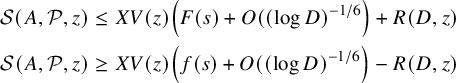 $$\begin{align*}\begin{aligned} {\mathcal S}(A, {\mathcal P}, z) \le X V(z)\left( F(s)+O(( \log D)^{-1/6}\right)+R(D,z)\\ {\mathcal S}(A, {\mathcal P}, z) \ge X V(z)\left( f(s)+O(( \log D)^{-1/6}\right)-R(D,z) \end{aligned} \end{align*}$$
for $s \ge \beta (\kappa )-1$
and
$s \ge \beta (\kappa )-1$
and $ s\ge \beta (\kappa )$
(resp.), where
$ s\ge \beta (\kappa )$
(resp.), where
 $$\begin{align*}R(D,z) \le \sum_{\substack{d \le D \\ d|P(z)}} |r_d| \end{align*}$$
and $\beta (\kappa )$
denotes the sifting limit of dimension
$\beta (\kappa )$
denotes the sifting limit of dimension $\kappa $
(cf. [Reference Friedlander and Iwaniec15, Ch. 6.4].)
$\kappa $
(cf. [Reference Friedlander and Iwaniec15, Ch. 6.4].)
In particular, note that for $\kappa =1/2$
(which is of particular interest to us since we sieve out by the density
$\kappa =1/2$
(which is of particular interest to us since we sieve out by the density $1/2$
sequence of primes
$1/2$
sequence of primes $ \equiv 3\ \pmod 4 $
to detect sums of two squares), it is well known that
$ \equiv 3\ \pmod 4 $
to detect sums of two squares), it is well known that $\beta (\kappa ) =1$
(e.g., see [Reference Friedlander and Iwaniec15, Ch. 14.2]), which will be important for us as the ‘sifting variable’ s (which measures the sifting range relative to the sifting level, for example, smaller s corresponds to a smaller sifting range) only needs to be
$\beta (\kappa ) =1$
(e.g., see [Reference Friedlander and Iwaniec15, Ch. 14.2]), which will be important for us as the ‘sifting variable’ s (which measures the sifting range relative to the sifting level, for example, smaller s corresponds to a smaller sifting range) only needs to be $\ge 1$
to provide a lower bound for
$\ge 1$
to provide a lower bound for ${\mathcal S}(A,{\mathcal P},z)$
, whereas for the linear sieve
${\mathcal S}(A,{\mathcal P},z)$
, whereas for the linear sieve $\beta (1)=2$
so that one needs
$\beta (1)=2$
so that one needs $s \ge 2$
. In our arguments, we will use
$s \ge 2$
. In our arguments, we will use $\beta $
-sieve weights, which are as defined in [Reference Friedlander and Iwaniec15] Sections 6.4–6.5. In particular for these weights, we have
$\beta $
-sieve weights, which are as defined in [Reference Friedlander and Iwaniec15] Sections 6.4–6.5. In particular for these weights, we have $|\lambda _d| \le 1$
. We will sometimes refer to the fundamental lemma of the sieve, by which we mean the following result (see [Reference Friedlander and Iwaniec15, Lemma 6.11].)
$|\lambda _d| \le 1$
. We will sometimes refer to the fundamental lemma of the sieve, by which we mean the following result (see [Reference Friedlander and Iwaniec15, Lemma 6.11].)
Theorem 2.2. Let $\Lambda ^{\pm }=\{ \lambda _d^{\pm } \}$
be upper and lower bound (resp.)
$\Lambda ^{\pm }=\{ \lambda _d^{\pm } \}$
be upper and lower bound (resp.) $\beta $
-sieves of level D with
$\beta $
-sieves of level D with $\beta \ge 4 \kappa +1$
. Also, let
$\beta \ge 4 \kappa +1$
. Also, let $s=\log D/\log z$
. Then for any multiplicative function satisfying equation (2.5) and
$s=\log D/\log z$
. Then for any multiplicative function satisfying equation (2.5) and $s \ge \beta +1$
we have
$s \ge \beta +1$
we have
 $$\begin{align*}\sum_{d|P(z)} \lambda_d^{\pm} g(d)=V(z)\left(1+O\left(s^{-s/2} \right) \right). \end{align*}$$
We also require the following estimate for the convolution of two sieves (see equation (5.97) and Theorem 5.9 of [Reference Friedlander and Iwaniec15]).
Theorem 2.3. Let $\Lambda _1=\{ \lambda _{d} \}$
and
$\Lambda _1=\{ \lambda _{d} \}$
and $\Lambda _2=\{ \lambda _{d}^{'} \}$
be upper-bound sieve weights of level
$\Lambda _2=\{ \lambda _{d}^{'} \}$
be upper-bound sieve weights of level $D_1,D_2$
(resp.). Also, let
$D_1,D_2$
(resp.). Also, let $g_1,g_2$
be multiplicative functions satisfying equation (2.5) with
$g_1,g_2$
be multiplicative functions satisfying equation (2.5) with $\kappa =1$
. Then
$\kappa =1$
. Then
 $$\begin{align*}\bigg|\sum_{\substack{d,e \\ (d,e)=1 }} \lambda_d \lambda_e^{'} g_1(d)g_2(e) \bigg| \le (4 e^{2\gamma}+o(1)) \prod_{p}(1+h_1(p)h_2(p)) \prod_{j=1}^2 \prod_{p < D_j} (1-g_j(p)) \end{align*}$$
as $\min \{D_1,D_2\} \rightarrow \infty $
, where for
$\min \{D_1,D_2\} \rightarrow \infty $
, where for $j=1,2$
,
$j=1,2$
, $ h_j(n)=g_j(n)(1-g_j(n))^{-1} $
and
$ h_j(n)=g_j(n)(1-g_j(n))^{-1} $
and $\gamma $
is Euler’s constant.
$\gamma $
is Euler’s constant.
If in addition $g_1(p), g_2(p) \le 1/p$
so that
$g_1(p), g_2(p) \le 1/p$
so that $h_1(p)h_2(p) \ll 1/p^2$
, which will be the case for us, then
$h_1(p)h_2(p) \ll 1/p^2$
, which will be the case for us, then
 $$ \begin{align} \bigg| \sum_{\substack{d,e \\ (d,e)=1 }} \lambda_d \lambda_e^{'} g_1(d)g_2(e) \bigg| \le C \prod_{p< D_1}(1-g_1(p))\prod_{p<D_2}(1-g_2(p)), \end{align} $$
where $C>0$
is an absolute constant.
$C>0$
is an absolute constant.
2.1.1 Notation
We will also use the notation
 $$\begin{align*}P_3(z_1,z_2):=\prod_{\substack{z_1 \le p \le z_2 \\ p \equiv 3\ \ \ \pmod 4}} p, \qquad \text{ and }\qquad P_3(z):=P_3(3,z). \end{align*}$$
Additionally, let $1(n)=1_{\mathbb N}(n)=1$
denote the identity function and let
$1(n)=1_{\mathbb N}(n)=1$
denote the identity function and let $\tau (n)=(1\ast 1)(n)=\sum _{d|n} 1$
. Also, define
$\tau (n)=(1\ast 1)(n)=\sum _{d|n} 1$
. Also, define
 $$ \begin{align} \mathcal B(x;q,a,\varepsilon) := \sum_{\substack{ x \le n \le 2x\\ n \equiv a\ \ \ {\pmod q}}} (1_{{{\mathcal P}}_{\varepsilon}} \ast 1_{{{\mathcal P}}_{\varepsilon}'})(n)-\frac{1}{\varphi(q)} \sum_{\substack{x \le n \le 2x \\ (n,q)=1}} (1_{{{\mathcal P}}_{\varepsilon}} \ast 1_{{{\mathcal P}}_{\varepsilon}'}) (n). \end{align} $$
Further, $\delta> 0$
will denote a small, but fixed real number.
$\delta> 0$
will denote a small, but fixed real number.
2.2 Preliminary lemmas
We begin by showing that the difference between the upper and lower bound sieves is ‘small’.
Lemma 2.1. Let $\Lambda ^{\pm }=\{ \lambda _d^{\pm }\}$
be upper and lower bound linear sieves (resp.) each of level
$\Lambda ^{\pm }=\{ \lambda _d^{\pm }\}$
be upper and lower bound linear sieves (resp.) each of level $w=x^{\sqrt {\eta }}$
, where
$w=x^{\sqrt {\eta }}$
, where $\eta>0$
is sufficiently small, whose sieve weights are supported on integers d such that
$\eta>0$
is sufficiently small, whose sieve weights are supported on integers d such that $d|P(y)$
, where
$d|P(y)$
, where $y=x^{\eta }$
,
$y=x^{\eta }$
, $y>Q_0Q_1$
, and
$y>Q_0Q_1$
, and $(d,2Q_0 f_1r_1)=1$
; in particular,
$(d,2Q_0 f_1r_1)=1$
; in particular,
 $$ \begin{align} \lambda_{d}^{\pm} = 0 \text{ if } (d,2Q_0 f_1r_1)> 1.\\[-9pt]\nonumber \end{align} $$
Then
 $$\begin{align*}\begin{aligned} &\sum_{\substack{x \le n \le 2x \\ Q_1|Q_0n+4}} \left((\lambda^+ \ast 1)\left(\frac{Q_0n+4}{Q_1}\right)-(\lambda^- \ast 1) \left(\frac{Q_0n+4}{Q_1}\right)\right) (1_{ {\mathcal P}_{\varepsilon}} \ast 1_{ {\mathcal P}_{\varepsilon}'})(n) \\ &\qquad \qquad \qquad \ll \varepsilon^{2} \eta^{1/(4\eta^{1/2})-1} \frac{Q_0}{\varphi(Q_0)} \frac{x \log \log x}{\varphi(Q_1) (\log x)^2}+\frac{x}{(\log x)^{10}}. \end{aligned}\\[-9pt] \end{align*}$$
Remark 2. We imposed the assumption that $\eta>0$
is sufficiently small so small that the error
$\eta>0$
is sufficiently small so small that the error $O(\eta ^{1/(4\eta ^{1/2})})$
in equation (2.16) is less than
$O(\eta ^{1/(4\eta ^{1/2})})$
in equation (2.16) is less than $1/2$
. The requirement
$1/2$
. The requirement $y>Q_0Q_1$
is not essential; in the case
$y>Q_0Q_1$
is not essential; in the case $y<Q_0Q_1$
the argument proceeds similarly, but some additional, straightforward estimates are needed to treat the contribution of the primes between y and
$y<Q_0Q_1$
the argument proceeds similarly, but some additional, straightforward estimates are needed to treat the contribution of the primes between y and $Q_0Q_1$
.
$Q_0Q_1$
.
Proof. Switching order of summation, it follows that
 $$ \begin{align} \begin{aligned} &\sum_{\substack{x \le n \le 2x \\ Q_1|Q_0n+4}} \left((\lambda^+ \ast 1)\left(\frac{Q_0n+4}{Q_1}\right)-(\lambda^- \ast 1) \left(\frac{Q_0n+4}{Q_1}\right)\right) (1_{ {\mathcal P}_{\varepsilon}} \ast 1_{ {\mathcal P}_{\varepsilon}'})(n) \\ & \qquad \qquad \qquad = \sum_{\pm} \pm \sum_{\substack{d <w \\ d|P(y) \\ (d,2Q_0f_1r_1)=1}}\lambda_d^{\pm} \sum_{\substack{x \le n \le 2x \\ Q_0n+4 \equiv 0\ \ \ {\pmod dQ_1}}} (1_{ {\mathcal P}_{\varepsilon}} \ast 1_{ {\mathcal P}_{\varepsilon}'})(n). \end{aligned}\\[-9pt]\nonumber \end{align} $$
The inner sum on the right-hand side (RHS) of equation (2.12) equals
 $$ \begin{align} \begin{aligned} &\frac{1}{\varphi(dQ_1)} \sum_{\substack{x\le n \le 2x \\ (n,dQ_1)=1}} (1_{ {\mathcal P}_{\varepsilon}} \ast 1_{ {\mathcal P}_{\varepsilon}'})(n)+\mathcal B\left(x; dQ_1, \gamma, \varepsilon \right), \end{aligned}\\[-9pt]\nonumber \end{align} $$
where $\gamma $
is the unique reduced residue
$\gamma $
is the unique reduced residue $\pmod {dQ_1}$
satisfying
$\pmod {dQ_1}$
satisfying $\gamma \cdot Q_0 \equiv -4\ \pmod {dQ_1}$
and
$\gamma \cdot Q_0 \equiv -4\ \pmod {dQ_1}$
and $\mathcal B$
is as defined in equation (2.10). Also,
$\mathcal B$
is as defined in equation (2.10). Also,
 $$ \begin{align} \sum_{\substack{ x\le n \le 2x \\ (n,dQ_1)=1}} (1_{ {\mathcal P}_{\varepsilon}} \ast 1_{ {\mathcal P}_{\varepsilon}'})(n)=\sum_{\substack{x \le n \le 2x }} (1_{ {\mathcal P}_{\varepsilon}} \ast 1_{ {\mathcal P}_{\varepsilon}'})(n)+O\bigg( \sum_{\substack{p_1p_2 \le 2x \\ (p_1p_2,dQ_1) \neq 1}}1_{ {\mathcal P}_{\varepsilon}}(p_1) 1_{ {\mathcal P}_{\varepsilon}'}(p_2) \bigg).\\[-9pt]\nonumber \end{align} $$
Since $dQ_1 \le x^{1/9}$
(as
$dQ_1 \le x^{1/9}$
(as $\eta $
is small) and
$\eta $
is small) and $p_2 \le x^{1/9}$
the contribution to the error term from
$p_2 \le x^{1/9}$
the contribution to the error term from $p_1p_2 \le x$
with
$p_1p_2 \le x$
with $p_1|(p_1p_2,dQ_1)$
is
$p_1|(p_1p_2,dQ_1)$
is $\ll \sum _{p_2 \le x^{1/9}} \sum _{p_1 \le x^{1/9} } 1 \ll x^{2/9}$
. Also, since
$\ll \sum _{p_2 \le x^{1/9}} \sum _{p_1 \le x^{1/9} } 1 \ll x^{2/9}$
. Also, since $p_2 \ge (\log x)^{B_0}$
 $$ \begin{align} \sum_{\substack{p_1p_2 \le 2x \\ (p_1p_2,dQ_1) = p_2}}1_{ {\mathcal P}_{\varepsilon}}(p_1) 1_{ {\mathcal P}_{\varepsilon}'}(p_2) \le \sum_{\substack{p_2|dQ_1 \\ p_2 \ge (\log x)^{B_0}}} \sum_{p_1 \le 2 x/p_2} 1 \ll \frac{x}{\log x} \sum_{\substack{p_2|dQ_1 \\ p_2 \ge (\log x)^{B_0}}} \frac{1}{p_2} \ll \frac{x (\log \log x)}{(\log x)^{B_0}}. \end{align} $$
Hence, using equations (2.13), (2.14) and (2.15) along with the fundamental lemma of the sieve (see Theorem 2.2 and recall $|\lambda _d|\le 1$
) with
$|\lambda _d|\le 1$
) with $g(d)=\varphi (Q_1)/\varphi (Q_1 d)$
,Footnote
2
and
$g(d)=\varphi (Q_1)/\varphi (Q_1 d)$
,Footnote
2
and $s=\log w/\log y=\eta ^{-1/2}$
we have that
$s=\log w/\log y=\eta ^{-1/2}$
we have that
 $$ \begin{align} \begin{aligned} &\sum_{\substack{d <w \\ d|P(y) \\ (d,2Q_0)=1}}\lambda_d^{\pm} \sum_{\substack{x \le n \le 2x \\ Q_0n+4 \equiv 0\ \ \ {\pmod dQ_1}}} (1_{ {\mathcal P}_{\varepsilon}} \ast 1_{ {\mathcal P}_{\varepsilon}'})(n)\\ &=\frac{1}{\varphi(Q_1)} \sum_{\substack{x \le n \le 2x }} (1_{ {\mathcal P}_{\varepsilon}} \ast 1_{ {\mathcal P}_{\varepsilon}'})(n) \prod_{\substack{p \le y \\ (p , 2Q_0f_1r_1 )=1}}\left(1-\frac{\varphi(Q_1)}{\varphi(Q_1p)} \right)(1+O(\eta^{1/(4\eta^{1/2})}))\\ & \qquad \qquad \qquad +O\bigg( \sum_{\substack{d < w \\ (d,2)=1}} \left|\mathcal B \left(x; dQ_1, \gamma, \varepsilon \right)\right|\bigg)+O\left( \frac{x \log \log x}{(\log x)^{B_0-1}}\right). \end{aligned}\\[-17pt]\nonumber \end{align} $$
Applying Theorem A.1 from the appendix, since $w=x^{\sqrt {\eta }} < x^{1/2-o(1)}$
we get that
$w=x^{\sqrt {\eta }} < x^{1/2-o(1)}$
we get that
 $$\begin{align*}\sum_{\substack{d < w \\ (d,2)=1}} \left|\mathcal B \left(x; dQ_1, \gamma, \varepsilon \right)\right| \ll \frac{x}{ (\log x)^{10}}.\\[-17pt] \end{align*}$$
Using the two estimates above in equation (2.12) (note the main terms in equation (2.16) are the same for each of the sieves $\Lambda ^{\pm }$
so they cancel in equation (2.12)) and applying equation (A.3) (with
$\Lambda ^{\pm }$
so they cancel in equation (2.12)) and applying equation (A.3) (with $q=1$
) from the appendix to estimate the sum over n completes the proof upon noting that
$q=1$
) from the appendix to estimate the sum over n completes the proof upon noting that
 $$\begin{align*}\prod_{\substack{p \le y \\ (p , 2Q_0f_1r_1)=1}}\left(1-\frac{\varphi(Q_1)}{\varphi(Q_1p)} \right) \asymp \frac{Q_0}{\varphi(Q_0) \log y} = \frac{Q_0}{\varphi(Q_0) \eta \log x}.\\[-56pt] \end{align*}$$
We next give a lower bound on the upper bound sieve, which together with Lemma 2.1 is strong enough (given suitable parameter choices) to show the existence of infinitely many integers with exactly two prime factors with the desired properties.
Lemma 2.2. Let $w = x^{\sqrt {\eta }}$
,
$w = x^{\sqrt {\eta }}$
, $y=x^{\eta }$
and
$y=x^{\eta }$
and $\Lambda ^{+}$
be as in Lemma 2.1. Let
$\Lambda ^{+}$
be as in Lemma 2.1. Let $\delta> 3 \sqrt {\eta }>0$
and
$\delta> 3 \sqrt {\eta }>0$
and $z=x^{\frac 12-\delta }$
. Then there exists a constant
$z=x^{\frac 12-\delta }$
. Then there exists a constant $C_1>0$
such that
$C_1>0$
such that
 $$\begin{align*}\sum_{\substack{x \le n \le 2x \\ (Q_0n+4, P_3(y,z))=1 \\ Q_1|Q_0n+4}} (1_{ {\mathcal P}_{\varepsilon}} \ast 1_{ {\mathcal P}_{\varepsilon}'}) (n) (\lambda^+ \ast 1)\left(\frac{Q_0n+4}{Q_1}\right) \ge C_1 \frac{\varepsilon^2 \delta^{1/2}}{\eta^{1/2}} \frac{Q_0}{\varphi(Q_0)} \frac{x \log \log x}{\varphi(Q_1)(\log x)^2}.\\[-15pt] \end{align*}$$
Proof. We now implement the sieve as discussed in Section 2. We start with the sifting sequence
 $$\begin{align*}\mathcal A=\bigg\{ (1_{ {\mathcal P}_{\varepsilon}} \ast 1_{ {\mathcal P}_{\varepsilon}'})\bigg(\frac{m-4}{Q_0}\bigg) (\lambda^+ \ast 1)\left(\frac{m}{Q_1}\right) : Q_1|m, Q_0|m-4 \bigg\}\\[-15pt] \end{align*}$$
and primes ${\mathcal P}=\{ p \ge y : p \equiv 3\ \pmod 4 \}$
. With (2.11) in mind, we may choose
${\mathcal P}=\{ p \ge y : p \equiv 3\ \pmod 4 \}$
. With (2.11) in mind, we may choose
 $$ \begin{align} \begin{aligned} X :=& \sum_{\substack{e<w \\ e|P(y)}} \frac{\lambda_e^+}{\varphi(eQ_1)} \sum_{\substack{x \le n \le 2x \\ (n, Q_1e)=1}} (1_{ {\mathcal P}_{\varepsilon}} \ast 1_{ {\mathcal P}_{\varepsilon}'})(n) \\ =&\sum_{\substack{x \le n \le 2x \\ (n, Q_1)=1}} (1_{ {\mathcal P}_{\varepsilon}} \ast 1_{ {\mathcal P}_{\varepsilon}'})(n) \sum_{\substack{e<w \\ e|P(y) \\ (e,2Q_0f_1r_1n)=1}} \frac{\lambda_e^+}{\varphi(eQ_1)}. \end{aligned} \end{align} $$
Arguing as in the proof of Lemma 2.1, to estimate the inner sum we apply the fundamental lemma of the sieve (see equation (2.16) and take $D=w$
,
$D=w$
, $z=y$
in Theorem 2.2 and note that we then have
$z=y$
in Theorem 2.2 and note that we then have $s=\eta ^{-1/2}$
) to get that it is
$s=\eta ^{-1/2}$
) to get that it is
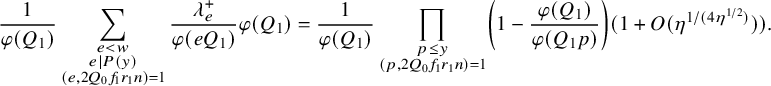 $$\begin{align*}\frac{1}{\varphi(Q_1)}\sum_{\substack{e<w \\ e|P(y) \\ (e,2Q_0f_1r_1n)=1}} \frac{\lambda_e^+}{\varphi(eQ_1)} \varphi(Q_1)= \frac{1}{\varphi(Q_1)}\prod_{\substack{p \le y \\ (p , 2Q_0f_1r_1 n )=1}}\left(1-\frac{\varphi(Q_1)}{\varphi(Q_1p)} \right)(1+O(\eta^{1/(4\eta^{1/2})})). \end{align*}$$
For $n=p_1p_2$
, recalling that
$n=p_1p_2$
, recalling that $f_1 \ll 1$
and
$f_1 \ll 1$
and $r_1$
is prime, the RHS above is
$r_1$
is prime, the RHS above is
 $$\begin{align*}\asymp \frac{1}{\varphi(Q_1)} \prod_{\substack{p \le y \\ (p,Q_0)=1}}\left(1-\frac{1}{p-1}\right) \asymp \frac{1}{\varphi(Q_1)} \cdot \frac{Q_0}{\varphi(Q_0)} \frac{1}{\log y}. \end{align*}$$
Using equations (2.14) and (2.15) along with the prime number theorem for Gaussian primes in sectors (see equations (A.1) and (A.3) in the appendix, with $q=1$
) yields
$q=1$
) yields
 $$\begin{align*}\sum_{\substack{x \le n \le 2x \\ (n, Q_1)=1}} (1_{ {\mathcal P}_{\varepsilon}} \ast 1_{ {\mathcal P}_{\varepsilon}'})(n) \sim 4 \varepsilon^2 \cdot \frac{x \log \log x}{ \log x}. \end{align*}$$
We conclude that
 $$ \begin{align} X \asymp \varepsilon^2 \frac{Q_0}{\varphi(Q_0)} \frac{x \log \log x}{ \varphi(Q_1) (\log y) (\log x)}. \end{align} $$
For $d|P_3(y,z)$
, note that
$d|P_3(y,z)$
, note that $(d, eQ_0 Q_1)=1$
for e such that
$(d, eQ_0 Q_1)=1$
for e such that $p|e \Rightarrow p< y$
, and
$p|e \Rightarrow p< y$
, and $(1_{ {\mathcal P}_{\varepsilon }} \ast 1_{ {\mathcal P}_{\varepsilon }'})(n)=0$
if
$(1_{ {\mathcal P}_{\varepsilon }} \ast 1_{ {\mathcal P}_{\varepsilon }'})(n)=0$
if $(d,n) \neq 1$
. To apply the sieve, we require an estimate for
$(d,n) \neq 1$
. To apply the sieve, we require an estimate for $A_d$
(cf. equations (2.3) and (2.4) for the definition of
$A_d$
(cf. equations (2.3) and (2.4) for the definition of $A_{d}$
) and recalling our choice for X and the definition of
$A_{d}$
) and recalling our choice for X and the definition of $\mathcal B$
in equation (2.10) it follows that
$\mathcal B$
in equation (2.10) it follows that
 $$ \begin{align} \begin{aligned} A_d(Q_0x+4)&:=\sum_{\substack{x \le n \le 2x \\ Q_1 | Q_0n+4 \\ Q_0n+4 \equiv 0\ \ \ {\pmod d}}} (1_{ {\mathcal P}_{\varepsilon}} \ast 1_{ {\mathcal P}_{\varepsilon}'})(n) (\lambda^+ \ast 1)\left(\frac{Q_0n+4}{Q_1}\right) \\ &= \sum_{\substack{e< w \\ e|P(y)}} \lambda_e^{+} \sum_{\substack{ x \le n \le 2x \\ Q_0n+4 \equiv 0\ \ \ {\pmod eQ_1} \\ Q_0n+4 \equiv 0\ \ \ {\pmod d}}} (1_{ {\mathcal P}_{\varepsilon}} \ast 1_{ {\mathcal P}_{\varepsilon}'})(n) \\ &=\sum_{\substack{e< w \\ e|P(y)}} \frac{\lambda_e^{+}}{\varphi(deQ_1)} \sum_{\substack{x \le n \le 2x \\ (n, Q_1 e)=1}} (1_{ {\mathcal P}_{\varepsilon}} \ast 1_{ {\mathcal P}_{\varepsilon}'})(n)+r_d =\frac{1}{\varphi(d)}X+r_d, \end{aligned} \end{align} $$
where
 $$ \begin{align} r_d \ll \sum_{\substack{e<w \\ (e,2)=1}} \left|\mathcal B(x;deQ_1, \gamma, \varepsilon)\right| \end{align} $$
and $\gamma $
is the unique residue class
$\gamma $
is the unique residue class $\pmod {deQ_1}$
with
$\pmod {deQ_1}$
with $Q_0 \gamma \equiv -4\ \pmod {eQ_1}$
and
$Q_0 \gamma \equiv -4\ \pmod {eQ_1}$
and $Q_0\gamma \equiv -4\ \pmod d$
; also note that
$Q_0\gamma \equiv -4\ \pmod d$
; also note that $(d,eQ_1)=1$
and
$(d,eQ_1)=1$
and $\mathcal B$
is as in equation (2.10).
$\mathcal B$
is as in equation (2.10).
Hence, the half-dimensional Rosser–Iwaniec sieve Theorem 2.1 with set of primes ${\mathcal P}=\{ p \equiv 3\ \pmod {4} : p>y\}$
(so that equation (2.21) holds with
${\mathcal P}=\{ p \equiv 3\ \pmod {4} : p>y\}$
(so that equation (2.21) holds with $\kappa =1/2$
), gives for any
$\kappa =1/2$
), gives for any $D \ge z$
with
$D \ge z$
with $s=\log D/\log z$
 $$ \begin{align} \begin{aligned} \sum_{\substack{x \le n \le 2x \\ (Q_0n+4, P_3(y,z))=1 \\ Q_1|Q_0n+4}} (1_{ {\mathcal P}_{\varepsilon}} \ast 1_{ {\mathcal P}_{\varepsilon}'}) (n) (\lambda^+ \ast 1)\left(\frac{Q_0n+4}{Q_1}\right)& \\ \ge X V(z)\left(f(s)+O\left(\frac{1}{(\log D)^{1/6}}\right)\right) &-\sum_{\substack{d < D \\ d|P_3(y,z)}} |r_d|, \end{aligned} \end{align} $$
where
 $$ \begin{align} V(z)=\prod_{\substack{y \le p \le z \\ p \equiv 3\ \pmod 4}} \left( 1-\frac{1}{p-1} \right) \asymp \sqrt{\frac{\log y}{\log z}} \asymp \eta^{1/2}. \end{align} $$
Taking $D=z^{1+\delta }$
, so
$D=z^{1+\delta }$
, so $s=1+\delta $
, we have by Theorem A.1, which is proved in the appendix, that (taking
$s=1+\delta $
, we have by Theorem A.1, which is proved in the appendix, that (taking $q=edQ_{1}$
)
$q=edQ_{1}$
)
 $$ \begin{align} \sum_{\substack{d < D \\ d|P_{3}(y,z)}} |r_d| \ll \sum_{ \substack{q < DQ_1w \\ (q,2)=1}}\left( \tau(q) \max_{(a,q)=1} |\mathcal B(x;q,a, \varepsilon)| \right)\ll \frac{x}{(\log x)^3}. \end{align} $$
Here, note that $DQ_1w < x^{\frac 12-\frac {\delta }{2}+\sqrt {\eta }}< x^{\frac 12-\frac {\delta }{6}}$
, and the contribution of the divisor function is handled by using Cauchy–Schwarz along with the trivial bound
$DQ_1w < x^{\frac 12-\frac {\delta }{2}+\sqrt {\eta }}< x^{\frac 12-\frac {\delta }{6}}$
, and the contribution of the divisor function is handled by using Cauchy–Schwarz along with the trivial bound $|\mathcal B(x;q,a, \varepsilon )| \ll x/q $
. Also, note that
$|\mathcal B(x;q,a, \varepsilon )| \ll x/q $
. Also, note that $f(t) \sim 2 \sqrt {\frac {e^{\gamma }}{\pi }} \cdot \sqrt {t-1}$
as
$f(t) \sim 2 \sqrt {\frac {e^{\gamma }}{\pi }} \cdot \sqrt {t-1}$
as $t \rightarrow 1^+$
(see the equation after (14.3) of [Reference Friedlander and Iwaniec15]), so
$t \rightarrow 1^+$
(see the equation after (14.3) of [Reference Friedlander and Iwaniec15]), so $f(s)=f(1+\delta ) \gg \sqrt {\delta }$
. Using this along with equations (2.17), (2.22) and (2.23) in equation (2.21) completes the proof.
$f(s)=f(1+\delta ) \gg \sqrt {\delta }$
. Using this along with equations (2.17), (2.22) and (2.23) in equation (2.21) completes the proof.
Sieving as in the previous lemma, we will now deduce the claimed upper bound in Proposition 2.1.
Lemma 2.3. Let $\eta>0$
be sufficiently small and
$\eta>0$
be sufficiently small and $y=x^{\eta }$
, with
$y=x^{\eta }$
, with $y>Q_0Q_1$
. Then
$y>Q_0Q_1$
. Then
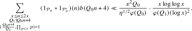 $$\begin{align*}\sum_{\substack{x \le n \le 2x \\ Q_1 | Q_0 n+4 \\ (\frac{Q_0n+4}{Q_1},\prod_{p \le y} p)=1}} (1_{ {\mathcal P}_{\varepsilon}} \ast 1_{ {\mathcal P}_{\varepsilon}'})(n) b(Q_0n+4) \ll \frac{ \varepsilon^{2} Q_0}{ \eta^{1/2} \varphi(Q_0)} \cdot \frac{x \log \log x}{ \varphi(Q_1) (\log x)^2}. \end{align*}$$
Proof. Write $Q_0n+4=Q_1 f^2 s$
, where s is square-free and note that since
$Q_0n+4=Q_1 f^2 s$
, where s is square-free and note that since $((Q_0n+4)/Q_1,P(y))=1$
all the prime divisors of f (and s as well) are
$((Q_0n+4)/Q_1,P(y))=1$
all the prime divisors of f (and s as well) are $\ge y$
, in particular f is coprime to
$\ge y$
, in particular f is coprime to $Q_0Q_1$
. We now note that
$Q_0Q_1$
. We now note that $b(s)\le 1_{S}(s)$
for
$b(s)\le 1_{S}(s)$
for $S=\{ n : (n,P_3(y,z))=1\}$
and take
$S=\{ n : (n,P_3(y,z))=1\}$
and take $\Lambda ^+$
to be the upper bound sieve from Lemma 2.1, which we use to bound the condition
$\Lambda ^+$
to be the upper bound sieve from Lemma 2.1, which we use to bound the condition $((Q_0n+4)/Q_1, \prod _{p \le y} p)=1$
to get that
$((Q_0n+4)/Q_1, \prod _{p \le y} p)=1$
to get that
 $$ \begin{align} \begin{aligned} & \sum_{\substack{x \le n \le 2x \\ Q_1 | Q_0 n+4 \\ (\frac{Q_0n+4}{Q_1},\prod_{p \le y} p)=1}} (1_{ {\mathcal P}_{\varepsilon}} \ast 1_{ {\mathcal P}_{\varepsilon}'})(n) b(Q_0n+4) \\ & \le \sum_{ \substack{f \le (\log x)^{10} \\ p|f \Rightarrow p>y}} \sum_{\substack{x\le n \le 2x \\ ((Q_0n+4)/f^2, P_3(y,z'))=1 \\ f^2Q_1|Q_0n+4}} (1_{ {\mathcal P}_{\varepsilon}} \ast 1_{ {\mathcal P}_{\varepsilon}'}) (n) (\lambda^+ \ast 1)\left(\frac{Q_0n+4}{Q_1}\right)+O(x/(\log x)^{10}), \end{aligned} \end{align} $$
where the error term arises from the contribution of $f> (\log x)^{10}$
. The following sieving argument is similar to the previous lemma (in fact we have already handled the case
$f> (\log x)^{10}$
. The following sieving argument is similar to the previous lemma (in fact we have already handled the case $f=1$
). For f as above let
$f=1$
). For f as above let
 $$ \begin{align} X_f:=\sum_{\substack{e<w \\ e|P(y)}} \frac{\lambda_e^+}{\varphi(eQ_1f^2)} \sum_{\substack{x \le n \le 2x \\ (n,f Q_1e)=1}} (1_{ {\mathcal P}_{\varepsilon}} \ast 1_{ {\mathcal P}_{\varepsilon}'})(n) \asymp \varepsilon^2 \frac{Q_0}{\varphi(Q_0)} \frac{x \log \log x}{\varphi(Q_1 f^2)(\log y) (\log x)}, \end{align} $$
where the last estimate follows from repeating the argument given in equation (2.18). Similarly, arguing as in equation (2.19) we have for each $d|P_{3}(y,z)$
with d coprime to f that
$d|P_{3}(y,z)$
with d coprime to f that
 $$\begin{align*}A_d(Qx+4;f):=\sum_{\substack{x \le n \le 2x \\ Q_1f^2 | Q_0n+4 \\ Q_0n+4 \equiv 0\ \ \ {\pmod d}}} (1_{ {\mathcal P}_{\varepsilon}} \ast 1_{ {\mathcal P}_{\varepsilon}'})(n) (\lambda^+ \ast 1)\left(\frac{Q_0n+4}{Q_1}\right) =\frac{1}{\varphi(d)} X_f+r_{d,f}, \end{align*}$$
where
 $$\begin{align*}r_{d,f} \ll \sum_{\substack{e<w \\ (e,2)=1}} \left|\mathcal B(x;def^2 Q_1, \gamma, \varepsilon)\right|. \end{align*}$$
We will now apply an upper bound sieve. For $D=x^{1/50}$
and
$D=x^{1/50}$
and $z'=x^{1/100}$
, Theorem 2.1 with set of primes
$z'=x^{1/100}$
, Theorem 2.1 with set of primes ${\mathcal P}=\{p \equiv 3\ \pmod 4: (p,f)=1 \, \& \, p>y\}$
gives for each
${\mathcal P}=\{p \equiv 3\ \pmod 4: (p,f)=1 \, \& \, p>y\}$
gives for each $f \le (\log x)^{10}$
with prime divisors all
$f \le (\log x)^{10}$
with prime divisors all $>y$
that the inner sum on the RHS of equation (2.24) is
$>y$
that the inner sum on the RHS of equation (2.24) is
 $$ \begin{align} \begin{aligned} & \le X_f V_f(z')\left(F(2)+O\left(\frac{1}{(\log D)^{1/6}}\right)\right)+\sum_{\substack{d < D \\ d|P_3(y,z), (d,f)=1}} |r_{d,f}|, \end{aligned} \end{align} $$
where the sum over d is $O(x^{1/25})$
since
$O(x^{1/25})$
since $D = x^{1/50}$
, and
$D = x^{1/50}$
, and
 $$ \begin{align} V_f(z')=\prod_{\substack{y \le p \le z' \\ p \equiv 3\ \ \ \pmod 4, \, p\nmid f}} \left(1-\frac{1}{p-1} \right)\ll \frac{f}{\varphi(f) } \eta^{1/2}, \end{align} $$
where the upper bound follows from equation (2.22). Using equations (2.25) and (2.27) in equation (2.26) then applying the resulting estimate in equation (2.24) and summing over f completes the proof.
2.3 The Proof of Proposition 2.1
We first require a Brun–Titchmarsh type bound for primes in narrow sectors.
Lemma 2.4. Let $Q, q\le x^{2/3-o(1)}$
be odd. Then
$Q, q\le x^{2/3-o(1)}$
be odd. Then
 $$\begin{align*}\sum_{ \substack{p=a^2+b^2 \le x \\ |\arctan(b/a)| \le \varepsilon \\ qp+4=Q p_1, \, p_1 \text{ prime} }} 1 \ll \varepsilon \frac{q}{\varphi(q)}\frac{x}{\varphi(Q)(\log x)^2}. \end{align*}$$
Remark 3. The point of the lemma is that it holds for large moduli $Q>x^{1/2}$
. To accomplish this, we use asymptotic estimates for Gaussian integers
$Q>x^{1/2}$
. To accomplish this, we use asymptotic estimates for Gaussian integers $\alpha =a+ib$
with
$\alpha =a+ib$
with $N(\alpha ) \le x$
and
$N(\alpha ) \le x$
and $N(\alpha ) \equiv a\ \pmod Q$
and
$N(\alpha ) \equiv a\ \pmod Q$
and $|\arg (\alpha )|\le \varepsilon $
, where
$|\arg (\alpha )|\le \varepsilon $
, where $N(\alpha )=\alpha \overline {\alpha }$
is the norm of
$N(\alpha )=\alpha \overline {\alpha }$
is the norm of $\alpha $
. Details are given in Appendix, cf. section A.2.
$\alpha $
. Details are given in Appendix, cf. section A.2.
The main step in the proof of Proposition 2.1 is the following lemma.
Lemma 2.5. Let $z=x^{\frac 12-\delta }$
, where
$z=x^{\frac 12-\delta }$
, where $\delta>0$
is sufficiently small and
$\delta>0$
is sufficiently small and $ y = x^{\eta }$
with
$ y = x^{\eta }$
with $0< \eta < 1/3$
. There exists a constant
$0< \eta < 1/3$
. There exists a constant $C_2>0$
such that
$C_2>0$
such that
 $$\begin{align*}\sum_{\substack{x \le n \le 2x \\ Q_1|Q_0n+4 \\ (\frac{Q_0n+4}{Q_1},P(y)P_3(y,z))=1}} (1_{{\mathcal P}_{\varepsilon}} \ast 1_{{\mathcal P}_{\varepsilon}'})(n) = \sum_{\substack{x \le n \le 2x \\ Q_1|Q_0n+4 \\ (\frac{Q_0n+4}{Q_1},P(y)) = 1 \\ p|Q_0n+4 \Rightarrow p \equiv 1\ \ \ {\pmod 4}}} (1_{{\mathcal P}_{\varepsilon}}\ast 1_{{\mathcal P}_{\varepsilon}'})(n)+R, \end{align*}$$
where
 $$\begin{align*}0 \le R \le C_2 \cdot \varepsilon^2 \cdot \frac{\delta^{3/2}}{\eta^{1/2}} \frac{Q_0}{\varphi(Q_0)} \cdot \frac{x \log \log x}{\varphi(Q_1)(\log x)^2}. \end{align*}$$
Proof. By construction, if $(1_{\mathcal P_{\varepsilon }} \ast 1_{ {\mathcal P}_{\varepsilon }'})(n) \neq 0$
, then
$(1_{\mathcal P_{\varepsilon }} \ast 1_{ {\mathcal P}_{\varepsilon }'})(n) \neq 0$
, then $Q_0n+4 \equiv 1\ \pmod 4$
and
$Q_0n+4 \equiv 1\ \pmod 4$
and $Q_1 \equiv 1\ \pmod 4$
so that
$Q_1 \equiv 1\ \pmod 4$
so that $(Q_0n+4)/Q_1 \equiv 1\ \pmod 4$
and must have an even number of prime factors which are congruent to
$(Q_0n+4)/Q_1 \equiv 1\ \pmod 4$
and must have an even number of prime factors which are congruent to $3\ \pmod 4$
. Since
$3\ \pmod 4$
. Since $z>x^{1/4}$
the integers which contribute to R must have precisely two such prime factors. Dropping several conditions on the integers n which contribute to R, it follows that R is bounded by the number of integers
$z>x^{1/4}$
the integers which contribute to R must have precisely two such prime factors. Dropping several conditions on the integers n which contribute to R, it follows that R is bounded by the number of integers $n=p_1p_2 \le 2x$
,
$n=p_1p_2 \le 2x$
, $( 1_{ {\mathcal P}_{\varepsilon }} \ast 1_{ \mathcal P_{\varepsilon }'})(n) \neq 0$
such that
$( 1_{ {\mathcal P}_{\varepsilon }} \ast 1_{ \mathcal P_{\varepsilon }'})(n) \neq 0$
such that $(Q_0n+4)/Q_1=aq_1q_2$
, where
$(Q_0n+4)/Q_1=aq_1q_2$
, where $b(a)=1$
,
$b(a)=1$
, $(a,P(y))=1$
,
$(a,P(y))=1$
, $q_1 \equiv q_2 \equiv 3\ \pmod 4$
and
$q_1 \equiv q_2 \equiv 3\ \pmod 4$
and $q_1,q_2$
are primes with
$q_1,q_2$
are primes with $z< q_1, q_2 \le 4Q_0x/Q_1$
so
$z< q_1, q_2 \le 4Q_0x/Q_1$
so $a \le 4Q_0x/(Q_1z^2)$
. By symmetry, it suffices to consider the terms with
$a \le 4Q_0x/(Q_1z^2)$
. By symmetry, it suffices to consider the terms with $q_1 \le q_2$
. We get that
$q_1 \le q_2$
. We get that
 $$ \begin{align} R \le 2 \sum_{p_2 \le (2x)^{1/9} } 1_{{\mathcal P}_{\varepsilon}'}(p_2) \sum_{\substack{ a \le \frac{4Q_0 x}{Q_{1}z^2} \\ (a,P(y))=1}} b(a) \sum_{z< q_1 \le \sqrt{\frac{4Q_0 x}{aQ_1}}} \sum_{q_1 \le q_2 \le 4Q_0x/Q_1} \sum_{\substack{p_1 \le 2x/p_2 \\ Q_0p_1p_2+4=aq_1q_2Q_1}} 1_{{\mathcal P}_{\varepsilon}}(p_1). \end{align} $$
Applying Lemma 2.4 with $q=Q_0p_2$
and
$q=Q_0p_2$
and $Q=aq_1Q_1$
,
$Q=aq_1Q_1$
,
 $$ \begin{align} \sum_{\substack{p_1 \le 2x/p_2 \\ Q_0p_1p_2+4=aq_1q_2Q_1}} 1_{{\mathcal P}_{\varepsilon}}(p_1) \ll \varepsilon \frac{Q_0}{\varphi(Q_0)}\frac{x}{ \varphi(aQ_1) q_1p_2 (\log x)^2}. \end{align} $$
Note that $x/p_2 \ge 2^{-1/9}x^{8/9}$
and
$x/p_2 \ge 2^{-1/9}x^{8/9}$
and $Q_0p_2, aq_1Q_1 \le \left ( \frac {x}{p_2}\right )^{2/3-o(1)}$
, for
$Q_0p_2, aq_1Q_1 \le \left ( \frac {x}{p_2}\right )^{2/3-o(1)}$
, for $\delta>0$
sufficiently small, so the application of Lemma 2.4 is valid.
$\delta>0$
sufficiently small, so the application of Lemma 2.4 is valid.
We claim that
 $$ \begin{align} \sum_{\substack{a \le \frac{4Q_0x}{Q_1z^2} \\ (a,P(y))=1}} \frac{b(a)}{\varphi(a)} \ll \sqrt{\frac{\log x/z^2}{\log y}}, \end{align} $$
which we will justify below. Additionally,
 $$ \begin{align} \sum_{z<q_1 \le \sqrt{\frac{4Q_0 x}{aQ_1}}} \frac{1}{q_1} \sim \log \frac{\log \sqrt{\frac{2Q_0 x}{aQ_1}}}{\log z} \ll \frac{\log \frac{ x}{z^2}}{\log z}+\frac{\log Q_0}{\log z} \ll \frac{\log \frac{ x}{z^2}}{\log z} \ll \delta. \end{align} $$
Therefore, using equations (2.29), (2.30) and (2.31) in equation (2.28) we conclude that
 $$\begin{align*}\begin{aligned} R \ll & \varepsilon \cdot \frac{Q_0}{\varphi(Q_0)} \cdot \frac{x \log x/z^2}{\varphi(Q_1) (\log x)^2 \log z} \sqrt{\frac{\log x/z^2}{\log y}} \sum_{p_2 \le (2x)^{1/9} } \frac{ 1_{{\mathcal P}_{\varepsilon}'}(p_2)}{p_2} \\ \ll & \varepsilon^2 \cdot \frac{\delta^{3/2}}{\eta^{1/2}}\cdot \frac{ Q_0}{ \varphi(Q_0)} \cdot \frac{x \cdot \log \log x }{\varphi(Q_1) (\log x)^2} \end{aligned} \end{align*}$$
as desired.
It remains to justify equation (2.30). Let $F(n)$
be the completely multiplicative function defined by
$F(n)$
be the completely multiplicative function defined by $F(p)=1$
if
$F(p)=1$
if $p \ge y$
and zero otherwise. Then for all
$p \ge y$
and zero otherwise. Then for all $t \ge y$
, it follows from basic estimates for multiplicative functions (see (1.85) of [Reference Iwaniec and Kowalski19]) that
$t \ge y$
, it follows from basic estimates for multiplicative functions (see (1.85) of [Reference Iwaniec and Kowalski19]) that
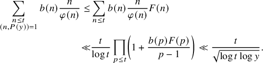 $$\begin{align*}\begin{aligned} \sum_{\substack{n \le t \\ (n,P(y))=1}} b(n) \frac{n}{\varphi(n)} \le& \sum_{\substack{n \le t }} b(n) \frac{n}{\varphi(n)} F(n) \\ \ll & \frac{t}{\log t} \prod_{ p \le t} \left(1+ \frac{b(p)F(p)}{p-1} \right) \ll \frac{t}{\sqrt{\log t \log y}}. \end{aligned} \end{align*}$$
For $1 \le t \le y$
, the sum on the left-hand side (LHS) is empty so the bound is true in that case as well. Hence, equation (2.30) follows from this estimate along with partial summation.
$1 \le t \le y$
, the sum on the left-hand side (LHS) is empty so the bound is true in that case as well. Hence, equation (2.30) follows from this estimate along with partial summation.
Proof of Proposition 2.1
The upper bound has already been established in Lemma 2.3. It remains to establish the lower bound. Let $\delta $
be sufficiently small in terms of
$\delta $
be sufficiently small in terms of $C_1$
and
$C_1$
and $C_2$
. Applying the inequality (2.7) for a lower bound sieve (also recall our notation (2.8)) along with Lemmas 2.1 and 2.2, using a lower bound sieve to take care of the condition
$C_2$
. Applying the inequality (2.7) for a lower bound sieve (also recall our notation (2.8)) along with Lemmas 2.1 and 2.2, using a lower bound sieve to take care of the condition $( \frac {Q_0n+4}{Q_1} , P(y)) = 1$
(and recalling that
$( \frac {Q_0n+4}{Q_1} , P(y)) = 1$
(and recalling that $z=x^{\frac 12-\delta }$
for
$z=x^{\frac 12-\delta }$
for $\delta>0$
), we have that
$\delta>0$
), we have that
 $$ \begin{align} \begin{aligned} \sum_{\substack{x \le n \le 2x \\ Q_1 |Q_0n+4 \\ (\frac{Q_0n+4}{Q_1},P(y)P_3(y,z))=1 }} (1_{ {\mathcal P}_{\varepsilon}} \ast 1_{ {\mathcal P}_{\varepsilon}'})(n) \ge& \sum_{\substack{ x \le n \le 2x \\ Q_1 |Q_0n+4\\ (Q_0n+4,P_3(y,z))=1}} (1_{ {\mathcal P}_{\varepsilon}} \ast 1_{ {\mathcal P}_{\varepsilon}'})(n) (\lambda^- \ast 1)\left(\frac{Q_0n+4}{Q_1}\right) \\ =& \sum_{\substack{ x \le n \le 2x \\ Q_1 |Q_0n+4\\ (Q_0n+4,P_3(y,z))=1}} (1_{ {\mathcal P}_{\varepsilon}} \ast 1_{ {\mathcal P}_{\varepsilon}'})(n) (\lambda^+ \ast 1)\left(\frac{Q_0n+4}{Q_1}\right)\\ &\qquad \qquad +O\left(\varepsilon^2 \eta^{1/(4\eta^{1/2})-1} \frac{Q_0}{\varphi(Q_0)} \frac{x \log \log x}{\varphi(Q_1)(\log x)^2} \right) \\ \ge& C_1 \frac{\varepsilon^2 \delta^{1/2}}{\eta^{1/2}} \frac{Q_0}{\varphi(Q_0)} \frac{x \log \log x}{\varphi(Q_1)(\log x)^2}\left(1+O\left( \frac{ \eta^{\frac{1}{4\eta^{1/2}}-\frac12}}{\delta^{1/2}} \right)\right). \end{aligned} \end{align} $$
Choosing $\eta $
sufficiently small in terms of
$\eta $
sufficiently small in terms of $\delta $
(which we choose in a way that only depends on
$\delta $
(which we choose in a way that only depends on $C_{1},C_{2}$
; see below) the O-term above is
$C_{1},C_{2}$
; see below) the O-term above is $ \le 1/2$
in absolute value. Therefore, by equation (2.32) along with Lemma 2.5 it follows that
$ \le 1/2$
in absolute value. Therefore, by equation (2.32) along with Lemma 2.5 it follows that
 $$ \begin{align*} \begin{aligned} \sum_{\substack{x \le n \le 2x \\ Q_1 |Q_0n+4 \\ (\frac{Q_0n+4}{Q_1},P(y)P_3(y,z))=1 \\ p|Q_0n+4 \Rightarrow p \equiv 1\ \ \ {\pmod 4 }}} (1_{ {\mathcal P}_{\varepsilon}} \ast 1_{ {\mathcal P}_{\varepsilon}'})(n) \ge \left(\frac{C_1}{2} \frac{\varepsilon^2 \delta^{1/2}}{\eta^{1/2}}-\frac{C_2 \varepsilon^2 \delta^{3/2}}{\eta^{1/2}} \right) \frac{Q_0}{\varphi(Q_0)} \frac{x \log \log x}{\varphi(Q_1)(\log x)^2}. \end{aligned} \end{align*} $$
The term $\left (\frac {C_1}{2} \delta ^{1/2}-C_2 \delta ^{3/2} \right )$
is positive for
$\left (\frac {C_1}{2} \delta ^{1/2}-C_2 \delta ^{3/2} \right )$
is positive for $\delta $
sufficiently small in terms of
$\delta $
sufficiently small in terms of $C_1$
and
$C_1$
and $C_2$
. Also,
$C_2$
. Also, $b(Q_0n+4) =1$
for n such that all the prime factors of
$b(Q_0n+4) =1$
for n such that all the prime factors of $Q_0n+4$
are congruent to
$Q_0n+4$
are congruent to $1\ \pmod 4$
. This completes the proof.
$1\ \pmod 4$
. This completes the proof.
3 Truncating the spectral equation
In this section, we show that it is possible to achieve a very short truncation of the spectral equation which holds for almost all new eigenvalues.
Theorem 3.1. Let $A \ge 1$
. Then for
$A \ge 1$
. Then for $B=B(A)$
sufficiently large, we have for every eigenvalue
$B=B(A)$
sufficiently large, we have for every eigenvalue $\lambda _n \in \Lambda _{new} \cap [1,x]$
except those outside an exceptional set of size
$\lambda _n \in \Lambda _{new} \cap [1,x]$
except those outside an exceptional set of size $O(x/(\log x)^A)$
that
$O(x/(\log x)^A)$
that
 $$ \begin{align} \sum_{m:|m-n| \le \frac{n}{x} (\log x)^B} \frac{r(m)}{m-\lambda_n} = \begin{cases} \pi \log \lambda_n+O(1)& \text{ in the weak coupling quantization},\\ \frac{1}{\alpha}+O(1) & \text{ in the strong coupling quantization}. \end{cases} \\[-17pt]\nonumber\end{align} $$
The above theorem is proved by capturing cancellation in the spectral equation even at very small scales for almost all new eigenvalues. This is done by showing that the average behavior of sums of $r(n)$
over even very short intervals is fairly regular.
$r(n)$
over even very short intervals is fairly regular.
Lemma 3.1. Let $x\ge 3$
and
$x\ge 3$
and $3 \le L \le x $
. Then
$3 \le L \le x $
. Then
 $$ \begin{align} \frac{1}{x} \sum_{ \ell \le x} \bigg| \sum_{\ell \le n \le \ell+\frac{\ell}{L}} r(n)-\pi \frac{\ell}{L} \bigg|^2 \ll \frac{x}{L} (\log x)^2.\\[-17pt]\nonumber \end{align} $$
Proof. We repeat a classical argument, which was used by Selberg [Reference Selberg41] to study primes in short intervals. Consider
 $$\begin{align*}\zeta_{\mathbb Q(i)}:= \frac14 \sum_{n \ge 1} \frac{r(n)}{n^s}=L(s,\chi_4) \zeta(s) \qquad \operatorname{Re}(s)>1,\\[-17pt] \end{align*}$$
where $L(s,\chi _4)$
is the Dirichlet L-function attached to the nontrivial Dirichlet character
$L(s,\chi _4)$
is the Dirichlet L-function attached to the nontrivial Dirichlet character $\pmod 4$
, and
$\pmod 4$
, and $\zeta (s)$
denotes the Riemann zeta-function. Note
$\zeta (s)$
denotes the Riemann zeta-function. Note $L(1, \chi _4)=\pi /4$
. Applying Perron’s formula, then shifting contours to
$L(1, \chi _4)=\pi /4$
. Applying Perron’s formula, then shifting contours to $\operatorname {Re}(s)=1/2$
(which is valid since it is well known that
$\operatorname {Re}(s)=1/2$
(which is valid since it is well known that $\zeta _{\mathbb Q(i)}(\sigma +it) \ll t^{1-\sigma +o(1)}$
, for
$\zeta _{\mathbb Q(i)}(\sigma +it) \ll t^{1-\sigma +o(1)}$
, for $0 \le \sigma \le 1$
) and picking up a simple pole at
$0 \le \sigma \le 1$
) and picking up a simple pole at $s=1$
we see that for
$s=1$
we see that for $v,v+v/L \notin \mathbb Z$
 $$\begin{align*}\begin{aligned} \sum_{v \le n \le v+\frac{v}{L}} r(n)& = \frac{1}{2\pi i} \int_{(2)} 4\zeta_{\mathbb Q(i)} (s) \frac{(v+\frac{v}{L})^s-v^s}{s} \, ds \\ & = 4 L(1,\chi_4) \cdot \frac{v}{L}+\frac{v^{1/2}}{2\pi} \int_{\mathbb R} 4 \zeta_{\mathbb Q(i)}(\tfrac12+it) \frac{(1+\frac{1}{L})^{\frac{1}{2}+it}-1}{\frac12+it} \cdot e^{i t \log v} \, dt. \end{aligned}\\[-17pt] \end{align*}$$
Notice that the integral on the RHS is a Fourier transform. Writing $\nu =\log (1+\frac 1L)$
, making a change of variables
$\nu =\log (1+\frac 1L)$
, making a change of variables $v=e^{\tau }$
and then applying Plancherel’s theorem yields
$v=e^{\tau }$
and then applying Plancherel’s theorem yields
 $$\begin{align*}\begin{aligned} \frac{1}{x^2} \int_1^{x} \bigg(\sum_{v \le n \le v+\frac{v}{L}} r(n)- \pi \cdot \frac{v}{L} \bigg)^2 \, dv \le & \int_{\mathbb R} \bigg(\sum_{e^{\tau} \le n \le e^{\tau+\nu}} r(n)- \pi \cdot \frac{e^{\tau}}{L} \bigg)^2 \frac{d\tau}{e^{\tau}} \\ =&\frac{8}{\pi} \int_{\mathbb R} |\zeta_{\mathbb Q(i)}(\tfrac12+it)|^2 |w_{\nu}(\tfrac12+it)|^2 \, dt, \end{aligned}\\[-17pt] \end{align*}$$
where $w_{\nu }(s)=(e^{\nu s}-1)/s \ll \min \{ \nu , 1/(1+|t|) \}$
uniformly for
$w_{\nu }(s)=(e^{\nu s}-1)/s \ll \min \{ \nu , 1/(1+|t|) \}$
uniformly for $\frac 14 \le \operatorname {Re}(s) \le 1$
. To estimate the integral on the RHS, we apply the well-known bound
$\frac 14 \le \operatorname {Re}(s) \le 1$
. To estimate the integral on the RHS, we apply the well-known bound
 $$\begin{align*}\int_0^{T} |\zeta_{\mathbb Q(i)} (\tfrac12+it)|^2 \, dt \ll T (\log T)^2 \end{align*}$$
(see the introduction of [Reference Müller32]). Hence, we see that
 $$\begin{align*}\begin{aligned} \int_{\mathbb R} |\zeta_{\mathbb Q(i)}(\tfrac12+it)|^2 |w_{\nu}(\tfrac12+it)|^2 \, dt \ll & \nu^2 \int_{|t| \le 1/\nu} |\zeta_{\mathbb Q(i)} (\tfrac12+it)|^2 \, dt+\int_{|t| \ge 1/\nu} |\zeta_{\mathbb Q(i)} (\tfrac12+it)|^2 \frac{dt}{t^2} \\ \ll & \nu (\log 1/\nu)^2 \ll \frac{1}{L} (\log L)^2. \end{aligned}\\[-9pt] \end{align*}$$
Combining the estimates above, we conclude that
 $$ \begin{align} \frac{1}{x} \int_{x}^{2x} \bigg( \sum_{v \le n \le v+\frac{v}{L}} r(n)-\pi \frac{v}{L} \bigg)^2 \, dv \ll \frac{x}{L} (\log x)^2.\\[-9pt]\nonumber \end{align} $$
We will now bound the sum over integers $ \ell \le x$
on the LHS of equation (3.2) in terms of an integral over
$ \ell \le x$
on the LHS of equation (3.2) in terms of an integral over $1 \le v \le x$
. Let
$1 \le v \le x$
. Let
 $$\begin{align*}F(v)=\sum_{v \le n \le v+\frac{v}{L}} r(n)- \pi \cdot \frac{v}{L},\\[-9pt] \end{align*}$$
and let $v_{\ell } \in [\ell , \ell +1]$
be a point where the minimum of
$v_{\ell } \in [\ell , \ell +1]$
be a point where the minimum of $|F(v)|$
on
$|F(v)|$
on $[\ell , \ell +1]$
is achieved. Observe that
$[\ell , \ell +1]$
is achieved. Observe that
 $$\begin{align*}F(\ell)=F(v_{\ell})+O\left( r(\ell)+r(\ell^*)+1 \right), \end{align*}$$
where $\ell ^*=\lfloor \ell +1+(\ell +1)/L \rfloor $
. Hence,
$\ell ^*=\lfloor \ell +1+(\ell +1)/L \rfloor $
. Hence,
 $$\begin{align*}\begin{aligned} \frac{1}{x}\sum_{ \ell \le x} F(\ell)^2 &\ll \frac{1}{x}\sum_{ \ell \le x} F(v_{\ell} )^2+\frac{1}{x}\sum_{\ell \le x }(r^2(\ell)+r^2(\ell^*))+1 \\ & \ll \frac{1}{x}\int_{1}^{x} F(x)^2 \, dx+ \log x \ll \frac{x}{L} (\log x)^2, \end{aligned}\\[-9pt] \end{align*}$$
where the last bound follows from equation (3.3) and the bound $\sum _{\ell \le x} r(l)^{2} \ll x \log x$
(which in turns follows from a Wirsing type estimate (cf. [Reference Wirsing49]) or by taking
$\sum _{\ell \le x} r(l)^{2} \ll x \log x$
(which in turns follows from a Wirsing type estimate (cf. [Reference Wirsing49]) or by taking $k=1$
,
$k=1$
, $R_{1}(X)=X$
and
$R_{1}(X)=X$
and $F_{1}(n) = r(n)$
in Lemma 4.1).
$F_{1}(n) = r(n)$
in Lemma 4.1).
Lemma 3.2. Let $A \ge 3$
and
$A \ge 3$
and $x,Y \ge 3$
. Then for all but
$x,Y \ge 3$
. Then for all but $\ll x/(\log x)^{A}$
integers
$\ll x/(\log x)^{A}$
integers $m \in [ 1, x]$
we have
$m \in [ 1, x]$
we have
 $$\begin{align*}\bigg| \sum_{Y \frac{m}{x} < k \le x^{1/2} \frac{m}{x}} \frac{r(m+k)-r(m-k)}{k} \bigg| \le \frac{(\log x)^{3A}}{\sqrt{Y}}. \end{align*}$$
Proof. Let
 $$\begin{align*}R_m(t)=\sum_{1 \le k \le t} (r(m+k)-r(m-k)). \end{align*}$$
It suffices to consider $m \in [x/(\log x)^A,x]$
. Hence, by summation by parts for each integer
$m \in [x/(\log x)^A,x]$
. Hence, by summation by parts for each integer $m \in [x/(\log x)^A,x]$
we have that
$m \in [x/(\log x)^A,x]$
we have that
 $$\begin{align*}\begin{aligned} \sum_{Y \frac{m}{x} < k \le x^{1/2} \frac{m}{x}} \frac{r(m+k)-r(m-k)}{k}=&\frac{R_m(x^{1/2} \frac{m}{x})}{x^{1/2} \frac{m}{x}}- \frac{R_m(Y \frac{m}{x})}{Y \frac{m}{x}}+\int_{Y \frac{m}{x}}^{x^{1/2} \frac{m}{x}} \frac{R_m(t)}{t^2} \, dt. \end{aligned} \end{align*}$$
Using this along with Chebyshev’s inequality and the elementary inequality $(|a|+|b|+|c|)^{2} \le 3^2 (a^2+b^2+c^2)$
, it follows that
$(|a|+|b|+|c|)^{2} \le 3^2 (a^2+b^2+c^2)$
, it follows that
 $$ \begin{align} \begin{aligned} & \# \left \{ \frac{x}{(\log x)^A} \le m \le x : \bigg| \sum_{Y \frac{m}{x} < k \le x^{1/3} \frac{m}{x}} \frac{r(m+k)-r(m-k)}{k} \bigg| \ge \frac{(\log x)^{3A}}{\sqrt{Y}} \right\} \\ & \le 9 \frac{Y}{(\log x)^{6A}} \sum_{ \frac{x}{(\log x)^A} \le m \le x} \left(\frac{R_m\left(x^{1/2} \frac{m}{x}\right)^2 (\log x)^{2A}}{x}+ \frac{R_m\left(Y \frac{m}{x}\right)^2 (\log x)^{2A}}{Y^2}+ \left(\int_{Y \frac{m}{x}}^{x^{1/2} \frac{m}{x}} \frac{R_m(t)}{t^2} \, dt \right)^2 \right). \end{aligned}\\[-9pt]\nonumber \end{align} $$
In the integral, we make a change of variables and apply the Cauchy–Schwarz inequality to get for each $m \in [x/(\log x)^A,x]$
that
$m \in [x/(\log x)^A,x]$
that
 $$ \begin{align} \left( \int_{Y \frac{m}{x}}^{x^{1/2} \frac{m}{x}} \frac{R_m(t)}{t^2} \, dt \right)^2\le \frac{(\log x)^{2A}}{Y} \int_{Y}^{x^{1/2}} \frac{1}{t^2} R_m\left( t\frac{m}{x}\right)^2 \, dt.\\[-9pt]\nonumber \end{align} $$
Observe that
 $$\begin{align*}R_m\left(H \frac{m}{x}\right)=\sum_{m \le n \le m+\frac{m}{x} H} r(n)-\sum_{m-\frac{m}{x} H \le n \le m} r(n).\\[-9pt] \end{align*}$$
Hence, by Lemma 3.1 with $L=x/H$
(along with an analogue of this lemma for the second sum, which is proved in the same way) we get
$L=x/H$
(along with an analogue of this lemma for the second sum, which is proved in the same way) we get
 $$\begin{align*}\frac{1}{x}\sum_{ m \le x}R_m\left(H \frac{m}{x}\right)^2 \ll H (\log x)^2, \end{align*}$$
for $1 \le H \le x/3$
. Using this bound and equation (3.5) in equation (3.4) gives
$1 \le H \le x/3$
. Using this bound and equation (3.5) in equation (3.4) gives
 $$\begin{align*}\begin{aligned} &\# \left \{ \frac{x}{(\log x)^A} \le m \le x : \bigg|\sum_{Y \frac{m}{x} < k \le x^{1/2} \frac{m}{x}} \frac{r(m+k)-r(m-k)}{k} \bigg| \ge \frac{(\log x)^{3A}}{\sqrt{Y}} \right\} \\ &\qquad \qquad \ll \frac{Y \cdot x}{(\log x)^{4A}}\left(\frac{(\log x)^2}{x^{1/2}}+\frac{(\log x)^2}{Y}+\frac{(\log x)^3}{Y} \right) \ll \frac{x}{(\log x)^{4A-3}} \end{aligned}\\[-9pt] \end{align*}$$
since we may assume $Y \le x^{1/2}$
, otherwise the set on the LHS above is empty.
$Y \le x^{1/2}$
, otherwise the set on the LHS above is empty.
Before proving the main result of this section, we require the following technical lemma.
Lemma 3.3. Let $u,v$
be sufficiently large positive real numbers such that
$u,v$
be sufficiently large positive real numbers such that $v^{9/10} \le u \le 2v$
. Let
$v^{9/10} \le u \le 2v$
. Let $t> 1$
be a real number that is not expressible as a sum of two squares such that
$t> 1$
be a real number that is not expressible as a sum of two squares such that $|u-t|\le v^{1/3}$
. Then
$|u-t|\le v^{1/3}$
. Then
 $$\begin{align*}\sum_{m:|m-u|> v^{\frac12}} r(m) \left(\frac{1}{m-t}-\frac{m}{m^2+1} \right)=-\pi \log t+O(1). \end{align*}$$
Proof. Let $A(x)=\sum _{1 \le n \le x} r(n)=\pi x+E(x)$
. It is well known that (cf. [Reference Sierpiński43]) that
$A(x)=\sum _{1 \le n \le x} r(n)=\pi x+E(x)$
. It is well known that (cf. [Reference Sierpiński43]) that $E(x) \ll x^{\frac 13}$
. Also, let
$E(x) \ll x^{\frac 13}$
. Also, let $f_t(x)=\log \frac {|x-t|}{(x^2+1)^{1/2}}$
, (so
$f_t(x)=\log \frac {|x-t|}{(x^2+1)^{1/2}}$
, (so $f_t(x) \rightarrow 0$
as
$f_t(x) \rightarrow 0$
as $x \rightarrow \infty $
). Since
$x \rightarrow \infty $
). Since $|u-t| \le v^{1/3}$
, partial summation gives
$|u-t| \le v^{1/3}$
, partial summation gives
 $$\begin{align*}\begin{aligned} \sum_{m:|m-u|> v^{\frac12}} r(m) \left(\frac{1}{m-t}-\frac{m}{m^2+1} \right)& = \int_{u+v^{\frac12}}^{\infty} f_t'(x) dA(x)+\int_{1^-}^{(u-v^{\frac12})^{-}} f_t'(x) dA(x) \\ & = \pi \left(f_t(u-v^{\frac12})-f_t(u+v^{\frac12})-\log t\right)\\ &\quad + O\left(1+\max_{\pm} \frac{u^{\frac13}}{|u\pm v^{\frac12}-t|} \right). \end{aligned} \end{align*}$$
The error is $O(1)$
since we assumed
$O(1)$
since we assumed $|u-t| \le v^{1/3}$
. Also,
$|u-t| \le v^{1/3}$
. Also,
 $$\begin{align*}f_t(u-v^{\frac12})-f_t(u+v^{\frac12})=\log \frac{|u-t-v^{\frac12}|}{|u-t+v^{\frac12}|}+O(1) \ll 1.\\[-48pt] \end{align*}$$
We are now ready to prove the main result of this section.
Proof of Theorem 3.1
Let $A \ge 1$
. In the weak coupling quantization, it follows from the spectral equation (1.1) along with Lemma 3.3 that
$A \ge 1$
. In the weak coupling quantization, it follows from the spectral equation (1.1) along with Lemma 3.3 that
 $$ \begin{align} \sum_{ m : |m-n| \le \frac{n}{x} x^{1/2}} \frac{r(m)}{m-\lambda_n}=\pi \log \lambda_n+O(1) \end{align} $$
for every integer $\frac {x}{(\log x)^A} \le n \le x$
, which is a sum of two squares. Note that the application of Lemma 3.3 is justified since it is well known that
$\frac {x}{(\log x)^A} \le n \le x$
, which is a sum of two squares. Note that the application of Lemma 3.3 is justified since it is well known that $\lambda _n-n \le n^+-n \le 10n^{1/4}$
(see for instance [Reference Montgomery and Vaughan31] p. 43).
$\lambda _n-n \le n^+-n \le 10n^{1/4}$
(see for instance [Reference Montgomery and Vaughan31] p. 43).
In the strong coupling quantization, applying Lemma 3.3 twice we get for $\frac {x}{(\log x)^A} \le n \le x$
that
$\frac {x}{(\log x)^A} \le n \le x$
that
 $$\begin{align*}\bigg| \sum_{m : |m-n|> \frac{n}{x} x^{1/2}} r(m) \left(\frac{1}{m-\lambda_n}-\frac{m}{m^2+1} \right) - \sum_{m :|m-\lambda_n| > \lambda_n^{1/2}} r(m) \left(\frac{1}{m-\lambda_n}-\frac{m}{m^2+1} \right)\bigg| \ll 1. \end{align*}$$
Hence, using this along with the spectral equation (1.2) we have
 $$\begin{align*}\begin{aligned} \sum_{|m-n| \le \frac{n}{x} x^{1/2}} r(m) \left(\frac{1}{m-\lambda_n}-\frac{m}{m^2+1} \right)=&\sum_{|m-\lambda_n| \le \lambda_n^{1/2}} r(m) \left(\frac{1}{m-\lambda_n}-\frac{m}{m^2+1} \right)+O(1) \\ =\,& \frac{1}{\alpha}+O(1). \end{aligned} \end{align*}$$
Hence, in the strong coupling quantization for each $\frac {x}{(\log x)^A} \le n \le x$
 $$ \begin{align} \sum_{ m : |m-n| \le \frac{n}{x} x^{1/2}} \frac{r(m)}{m-\lambda_n} = \frac{1}{\alpha}+O(1). \end{align} $$
For $\frac {x}{(\log x)^A} \le n \le x$
, we now analyze the sum that appears on the LHS of both equations (3.6) and (3.7). Let
$\frac {x}{(\log x)^A} \le n \le x$
, we now analyze the sum that appears on the LHS of both equations (3.6) and (3.7). Let $B \ge 1$
, to be determined later, and consider
$B \ge 1$
, to be determined later, and consider
 $$ \begin{align} \sum_{|m-n|\le \frac{n}{x} x^{1/2}} \frac{r(m)}{m-\lambda_n}= \sum_{|m-n|\le \frac{n}{x}(\log x)^B} \frac{r(m)}{m-\lambda_n}+ \sum_{ \frac{n}{x}(\log x)^B < |k| \le \frac{n}{x} x^{1/2} } \frac{r(n+k)}{k-{s_n}}, \end{align} $$
where recall ${s_n}=\lambda _n-n$
. Note that
${s_n}=\lambda _n-n$
. Note that
 $$\begin{align*}\begin{aligned} \sum_{\substack{n \le x \\ {s_n} \ge (\log x)^{B/2}}} b(n) \le & \frac{1}{(\log x)^{B/2}} \sum_{n \le x} b(n){s_n} \\ \le & \frac{1}{(\log x)^{B/2}} \sum_{n \le x} b(n) (n^+-n) \ll \frac{x}{(\log x)^{B/2}}. \end{aligned} \end{align*}$$
Hence, for all but $O(x/(\log x)^{B/2})$
integers
$O(x/(\log x)^{B/2})$
integers $n \le x$
which are representable as a sum of two squares,
$n \le x$
which are representable as a sum of two squares, ${s_n} < (\log x)^{B/2}$
. For these integers, the second sum on the RHS of equation (3.8) equals
${s_n} < (\log x)^{B/2}$
. For these integers, the second sum on the RHS of equation (3.8) equals
 $$ \begin{align} \sum_{ \frac{n}{x}(\log x)^B \le k \le \frac{n}{x}x^{1/2} } \frac{r(n+k)-r(n-k)}{k}+O\left( (\log x)^{B/2} \sum_{ \frac{n}{x}(\log x)^B \le |k| \le x^{1/2}} \frac{r(n+k)}{k^2} \right). \end{align} $$
Since
 $$\begin{align*}\begin{aligned} &\# \bigg\{ \frac{x}{(\log x)^A} \le n \le x : (\log x)^{B/2} \sum_{\frac{n}{x}(\log x)^B \le |k| \le x^{1/2}} \frac{r(n+k)}{k^2} \ge 1 \bigg\}\\ &\le (\log x)^{B/2} \sum_{(\log x)^{B-A} \le |k| \le x^{1/2}} \frac{1}{k^2}\sum_{ n \le x} r(n+k) \ll \frac{x}{(\log x)^{B/2-A}} \end{aligned} \end{align*}$$
the O-term in equation (3.9) is $\ll 1$
for all but
$\ll 1$
for all but $O(x/(\log x)^{B/2-A})$
integers
$O(x/(\log x)^{B/2-A})$
integers $\frac {x}{(\log x)^A} \le n \le x$
. The first sum in equation (3.9) is estimated using Lemma 3.2, with
$\frac {x}{(\log x)^A} \le n \le x$
. The first sum in equation (3.9) is estimated using Lemma 3.2, with $Y=(\log x)^B$
; so for
$Y=(\log x)^B$
; so for $B \ge 6A$
, this sum is
$B \ge 6A$
, this sum is $\ll 1$
for all but at most
$\ll 1$
for all but at most $\ll x/(\log x)^{A}$
integers
$\ll x/(\log x)^{A}$
integers $n \le x$
. Hence, applying the two previous estimates in equation (3.9) and using the resulting bound along with equation (3.8) in equations (3.6) and (3.7) completes the proof upon taking
$n \le x$
. Hence, applying the two previous estimates in equation (3.9) and using the resulting bound along with equation (3.8) in equations (3.6) and (3.7) completes the proof upon taking $B \ge 6A$
.
$B \ge 6A$
.
4 Estimates for new eigenvalues nearby almost primes
In this section, we analyze the location of eigenvalues in $\Lambda _{\text {new}}$
nearby certain integers which are almost primes. To state the result, let
$\Lambda _{\text {new}}$
nearby certain integers which are almost primes. To state the result, let
 $$ \begin{align} \begin{aligned} {\mathcal N}_{1,x}=&\{ n \in \mathbb N : (1_{ {\mathcal P}_{\varepsilon,x}} \ast 1_{ {\mathcal P}_{\varepsilon,x}'})(n) \neq 0, \, b(Q_0n+4)=1, \, \& \, \, Q_1 | Q_0n+4\}, \\ {\mathcal N}_{2,x}=&\left\{ n \in {\mathcal N}_{1,x} : \left(\frac{Q_0n+4}{Q_1}, P(y)\right)=1\right\}, \end{aligned} \end{align} $$
where $y=x^{\eta }$
with
$y=x^{\eta }$
with $\eta $
as in Proposition 2.1 and
$\eta $
as in Proposition 2.1 and $Q_0,Q_1, \varepsilon , 1_{{\mathcal P}_{\varepsilon }}$
and
$Q_0,Q_1, \varepsilon , 1_{{\mathcal P}_{\varepsilon }}$
and $b(\cdot )$
are as defined in the beginning of Section 2; we will write
$b(\cdot )$
are as defined in the beginning of Section 2; we will write ${\mathcal N}_{1,x}={\mathcal N}_1, {\mathcal N}_{2,x}={\mathcal N}_2$
for brevity. For
${\mathcal N}_{1,x}={\mathcal N}_1, {\mathcal N}_{2,x}={\mathcal N}_2$
for brevity. For $j=1,2$
, let
$j=1,2$
, let ${\mathcal N}_{j}(x)={\mathcal N}_{j,x} \cap [x,2x]$
. In particular, for each
${\mathcal N}_{j}(x)={\mathcal N}_{j,x} \cap [x,2x]$
. In particular, for each $n \in {\mathcal N}_2(x)$
,
$n \in {\mathcal N}_2(x)$
, $Q_0n+4=Q_1 \mathcal \ell _n$
, where
$Q_0n+4=Q_1 \mathcal \ell _n$
, where $\ell _n$
is an integer which is a sum of two squares. Moreover, since every prime divisor of
$\ell _n$
is an integer which is a sum of two squares. Moreover, since every prime divisor of $\ell _n$
is
$\ell _n$
is $\ge y=x^{\eta }$
, we have for
$\ge y=x^{\eta }$
, we have for $n \le x$
that
$n \le x$
that $ x^{ \eta \cdot \# \{ p| \ell _n\}} \le \ell _n \le 2Q_0x$
and
$ x^{ \eta \cdot \# \{ p| \ell _n\}} \le \ell _n \le 2Q_0x$
and
 $$ \begin{align} \# \{ p| \ell_n\} \le \frac{2}{\eta}. \end{align} $$
Note that by Propositions 2.1 and 2.2
 $$ \begin{align} \begin{aligned} \# {\mathcal N}_1(x) \asymp & \varepsilon^2 \frac{1}{\varphi(Q_1)} \frac{x \log \log x}{(\log x)^{3/2}}, \\ \# {\mathcal N}_2(x) \asymp & \varepsilon^2 \frac{Q_0}{\varphi(Q_0 Q_1)} \frac{x \log \log x}{(\log x)^2}. \end{aligned} \end{align} $$
The main result of this section is the following proposition.
Proposition 4.1. For all $n \in {\mathcal N}_j(x)$
,
$n \in {\mathcal N}_j(x)$
, $j=1,2$
, apart for elements in an exceptional set of size
$j=1,2$
, apart for elements in an exceptional set of size
 $$\begin{align*}\ll \frac{\# {\mathcal N}_j(x)}{ \varepsilon^2 (\log \log x)^{1-o(1)}} \end{align*}$$
we have for $m=Q_0n$
that
$m=Q_0n$
that $m^+=m+4$
and
$m^+=m+4$
and
 $$\begin{align*}\begin{aligned} &\frac{r(m)}{m-\lambda_m}+\frac{r(m^+)}{m^+-\lambda_m} \\ & \qquad \qquad =\begin{cases} \pi \log \lambda_m+O\left( (\log \log x)^5 \right) & \text{ in the weak coupling quantization},\\ O\left( (\log \log x)^5 \right) & \text{ in the strong coupling quantization}. \end{cases} \end{aligned} \end{align*}$$
We also require a sieve estimate for averages of correlations of multiplicative functions. The following result is due to Henriot [Reference Henriot17], which builds on the work of Nair and Tenenbaum [Reference Nair and Tenenbaum33]. See Corollary 1 of [Reference Henriot17] and the subsequent remark therein. Recall that $\tau (n)=\sum _{d|n}1$
denotes the divisor function, and for a polynomial
$\tau (n)=\sum _{d|n}1$
denotes the divisor function, and for a polynomial $R =\sum a_n X^n \in \mathbb Z[X]$
, let
$R =\sum a_n X^n \in \mathbb Z[X]$
, let $\lVert R \rVert _1=\sum |a_n|$
denote the norm of R.
$\lVert R \rVert _1=\sum |a_n|$
denote the norm of R.
Lemma 4.1. Let $R_1(X),\ldots , R_k( X) \in \mathbb Z[ X]$
be irreducible, pairwise coprime polynomials, for which each polynomial
$R_1(X),\ldots , R_k( X) \in \mathbb Z[ X]$
be irreducible, pairwise coprime polynomials, for which each polynomial $R_j$
does not have a fixed prime divisor.Footnote
3
Let D be the discriminant of
$R_j$
does not have a fixed prime divisor.Footnote
3
Let D be the discriminant of $R=R_1\cdots R_k$
and
$R=R_1\cdots R_k$
and $\varrho _{R_j}(n)=\# \{ a\ \pmod n: R_j(a) \equiv 0\ \pmod n\}$
. Then there exist
$\varrho _{R_j}(n)=\# \{ a\ \pmod n: R_j(a) \equiv 0\ \pmod n\}$
. Then there exist $C,c_0>0$
such that for any nonnegative multiplicative functions
$C,c_0>0$
such that for any nonnegative multiplicative functions $F_j$
,
$F_j$
, $j=1, \ldots , k$
with
$j=1, \ldots , k$
with $F_j(n) \le \tau (n)^{{E}}$
for some
$F_j(n) \le \tau (n)^{{E}}$
for some ${E} \ge 1$
, we have for
${E} \ge 1$
, we have for $x \ge c_0 \lVert R \rVert _1^{1/10} $
and some
$x \ge c_0 \lVert R \rVert _1^{1/10} $
and some $A \ge 1$
that
$A \ge 1$
that
 $$\begin{align*}\sum_{n \le x} \prod_{j=1}^k F_j(|R_j(n)|) \ll \Delta_D^{C} \, x \prod_{p \le x} \left(1-\frac{\varrho_{R}(p)}{p} \right) \prod_{j=1}^k \left(\sum_{n \le x} \frac{F_j(n) \varrho_{R_j}(n)}{n}\right), \end{align*}$$
where
 $$\begin{align*}\Delta_D :=\prod_{p|D}\left(1+\frac{1}{p} \right) \end{align*}$$
and the implicit constant, C and $c_0$
depend at most on the degree of R and
$c_0$
depend at most on the degree of R and ${E}$
.
${E}$
.
We first start with a technical lemma.
Lemma 4.2. Let f be a nonnegative multiplicative function with $f(n) {\,\le\,} \tau (n)$
and
$f(n) {\,\le\,} \tau (n)$
and $f(mn) {\,\le\,} \max \{1,f(n)\} f(m)$
for
$f(mn) {\,\le\,} \max \{1,f(n)\} f(m)$
for $m \in \mathbb N$
and n such that
$m \in \mathbb N$
and n such that $b(n)=1$
. Then for
$b(n)=1$
. Then for $1 {\,\le\,} |h| {\,\le\,} x^{1/30}$
, with
$1 {\,\le\,} |h| {\,\le\,} x^{1/30}$
, with $h {\,\neq\,} 4$
and
$h {\,\neq\,} 4$
and $j=1,2$
, we have
$j=1,2$
, we have
 $$ \begin{align} \begin{aligned} \sum_{n \in {\mathcal N}_j(x)} f(Q_0n+h) \ll \frac{1}{\varepsilon^2} \cdot g(h) \prod_{p|Q_0Q_1} \left(1+\frac{1}{p} \right)^C \prod_{p \le x} \left(1+\frac{f(p)-1}{p} \right) \# {\mathcal N}_j(x), \end{aligned} \end{align} $$
where $C>0$
is an absolute constant and
$C>0$
is an absolute constant and
 $$\begin{align*}g(h)=\tau(|h|)\tau(|h-4|)\prod_{p|h} \left(1+\frac{1}{p} \right)^C\prod_{p|h-4} \left(1+\frac{1}{p} \right)^C. \end{align*}$$
Additionally, (for $h=4$
) there exists
$h=4$
) there exists $C>0$
such that
$C>0$
such that
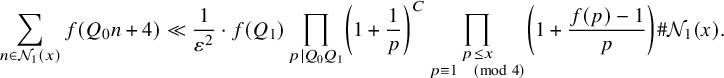 $$\begin{align*}\sum_{n \in {\mathcal N}_1(x)} f(Q_0n+4) \ll \frac{1}{\varepsilon^2} \cdot f(Q_1) \prod_{p|Q_0Q_1}\left(1+\frac{1}{p} \right)^C \prod_{\substack{p \le x \\ p \equiv 1\ \ \ {\pmod 4}}} \left(1+\frac{f(p)-1}{p} \right) \# {\mathcal N}_1(x).\\[-9pt] \end{align*}$$
Remark 4. When applying this lemma, we will take $f(n)=\tfrac 14 \cdot r(n),b(n)$
or
$f(n)=\tfrac 14 \cdot r(n),b(n)$
or $2^{-\omega _1(n)}$
, where
$2^{-\omega _1(n)}$
, where $\omega _1(n)=\# \{ p|n : p \equiv 1\ \pmod 4\}$
. The hypotheses of the lemma are satisfied for each of these choices.
$\omega _1(n)=\# \{ p|n : p \equiv 1\ \pmod 4\}$
. The hypotheses of the lemma are satisfied for each of these choices.
Proof. Let $T_j=2$
if
$T_j=2$
if $j=1$
and
$j=1$
and $T_j=y=x^{\eta }$
if
$T_j=y=x^{\eta }$
if $j=2$
. Dropping several of the conditions on
$j=2$
. Dropping several of the conditions on $n \in {\mathcal N}_j$
, we get that (here
$n \in {\mathcal N}_j$
, we get that (here $q< p$
denote primes; also recall that
$q< p$
denote primes; also recall that $P(z)$
is defined in equation (2.2))
$P(z)$
is defined in equation (2.2))
 $$ \begin{align} \begin{aligned} \sum_{n \in {\mathcal N}_j(x/2)} f(Q_0n+h) \le 2 \sum_{\substack{q \le \sqrt{x} \\ q\equiv 1\ \ \ {\pmod 4}}} \sum_{\substack{p \le x/q \\ Q_1 | Q_0pq+4 \\ (\frac{Q_0pq+4}{Q_1}, P(T_j))=1}} b(Q_0qp+4)f(Q_0qp+h). \end{aligned}\\[-12pt]\nonumber \end{align} $$
Let $K=Q_0q$
and
$K=Q_0q$
and $Y=x/q$
. Note that the sum above is empty unless
$Y=x/q$
. Note that the sum above is empty unless $(K,Q_1)=1$
. Since
$(K,Q_1)=1$
. Since $(K, Q_1)=1$
, there exist integers
$(K, Q_1)=1$
, there exist integers $\overline {K},\overline Q_1$
with
$\overline {K},\overline Q_1$
with $1 \le | \overline {K}| < Q_1$
and
$1 \le | \overline {K}| < Q_1$
and $1 \le |\overline {Q_1}| < K$
such that
$1 \le |\overline {Q_1}| < K$
such that $K \overline K -Q_1\overline Q_1=1$
. Also, for
$K \overline K -Q_1\overline Q_1=1$
. Also, for $Z \ge 1$
let
$Z \ge 1$
let $F_Z$
be the totally multiplicative function given by
$F_Z$
be the totally multiplicative function given by $F_Z(p)=1$
if
$F_Z(p)=1$
if $p \ge Z$
and zero otherwise. The inner sum on the RHS of equation (4.5) is bounded by
$p \ge Z$
and zero otherwise. The inner sum on the RHS of equation (4.5) is bounded by
 $$ \begin{align} \begin{aligned} \ll& \sum_{\substack{n \le Y, Q_1|Kn+4}} F_{\sqrt{Y}}(n)F_{T_j}\left(\frac{Kn+4}{Q_1} \right)b(Kn+4)f(Kn+h)+Y^{1/2+o(1)} \\ =& \sum_{\substack{m \le \frac{Y-4 \overline{K}}{Q_1}}} F_{\sqrt{Y}}(Q_1m-4\overline{K})F_{T_j}\left(Km-4\overline{Q_1} \right)b(KQ_1m-4Q_1\overline{Q_1})f(KQ_1m+h-4K\overline{K})\\ &+O(Y^{1/2+o(1)}) , \end{aligned}\\[-9pt]\nonumber \end{align} $$
where the error term $Y^{1/2+o(1)}$
accounts for the primes
$Y^{1/2+o(1)}$
accounts for the primes $p {\,\le\,} \sqrt {Y}$
. First, note
$p {\,\le\,} \sqrt {Y}$
. First, note $b(KQ_1n-4Q_1\overline {Q_1})=b(Kn-4\overline {Q_1})$
. Let
$b(KQ_1n-4Q_1\overline {Q_1})=b(Kn-4\overline {Q_1})$
. Let $d=(KQ_1,h-4K\overline K)$
, and suppose that
$d=(KQ_1,h-4K\overline K)$
, and suppose that $h \neq 4$
. We have
$h \neq 4$
. We have
 $$\begin{align*}f(KQ_1m+h-4K\overline{K}) \le \max\{1, f(d)\} f\left(\frac{KQ_1}{d}m+\frac{h-4K\overline{K}}{d}\right).\\[-9pt] \end{align*}$$
Let $R_1(X)=Q_1 X-4 \overline K$
,
$R_1(X)=Q_1 X-4 \overline K$
, $R_2(X)=K X-4 \overline Q_1$
,
$R_2(X)=K X-4 \overline Q_1$
, $R_3( X)=\frac {KQ_1}{d} X+\frac {h-4K\overline K}{d}$
and D denote the discriminant of
$R_3( X)=\frac {KQ_1}{d} X+\frac {h-4K\overline K}{d}$
and D denote the discriminant of $R=R_1R_2R_3$
. The polynomials
$R=R_1R_2R_3$
. The polynomials $R_1,R_2,R_3$
and multiplicative functions
$R_1,R_2,R_3$
and multiplicative functions $F_1=F_{\sqrt {Y}}$
,
$F_1=F_{\sqrt {Y}}$
, $F_2=F_{T_j}\cdot b$
and
$F_2=F_{T_j}\cdot b$
and $F_3=f$
satisfy the assumptions of Lemma 4.1. Also, for
$F_3=f$
satisfy the assumptions of Lemma 4.1. Also, for $(p,KQ_1)=1$
we have
$(p,KQ_1)=1$
we have $\varrho _R(p)=3$
and
$\varrho _R(p)=3$
and $\varrho _{R_j}(p^k)=1$
for each
$\varrho _{R_j}(p^k)=1$
for each $j=1,2,3$
and
$j=1,2,3$
and $k \ge 1$
, which follows from Hensel’s lemma. Hence, the sum in equation (4.6) is bounded by
$k \ge 1$
, which follows from Hensel’s lemma. Hence, the sum in equation (4.6) is bounded by
 $$\begin{align*}\begin{aligned} \ll & \max\{1,f(d)\} \Delta_{D}^{C} \frac{Y}{Q_1} \prod_{p \le Y} \left(1+\frac{F_{\sqrt{Y}}(p)+F_{T_j}(p)b(p)+f(p)-3}{p} \right) \prod_{p|KQ_1}\left( 1+\frac{1}{p}\right)^C \\ \ll & \max\{1,f(d)\} \Delta_{D}^{C} \prod_{p|KQ_1}\left(1+\frac{1}{p} \right)^C \frac{Y}{Q_1(\log Y)^{3/2}(\log T_j)^{1/2}} \prod_{p \le Y} \left( 1+\frac{f(p)-1}{p}\right). \end{aligned} \end{align*}$$
Write $d=p_1^{a_1} \cdots p_{\ell }^{a_\ell }$
. For each
$d=p_1^{a_1} \cdots p_{\ell }^{a_\ell }$
. For each $j=1, \ldots , \ell $
, we have
$j=1, \ldots , \ell $
, we have $p_j^{a_j}|h$
or
$p_j^{a_j}|h$
or $p_j^{a_j}|h-4$
(depending on whether
$p_j^{a_j}|h-4$
(depending on whether $p_j^{a_j}|K$
or
$p_j^{a_j}|K$
or $p_j^{a_j}|Q_1$
, respectively); so
$p_j^{a_j}|Q_1$
, respectively); so $f(d) \ll \tau (|h|)\tau (|h-4|)$
. Note the discriminant of R equals
$f(d) \ll \tau (|h|)\tau (|h-4|)$
. Note the discriminant of R equals $D=16 \frac {K^2Q_1^2}{d^4}h^2(h-4)^2$
so that
$D=16 \frac {K^2Q_1^2}{d^4}h^2(h-4)^2$
so that
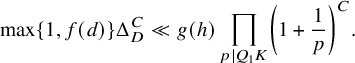 $$\begin{align*}\max\{1,f(d)\} \Delta_D^{C} \ll g(h) \prod_{p|Q_1K}\left(1+\frac{1}{p} \right)^C. \end{align*}$$
Also, since $Y =x/q\ge \sqrt {x}$
,
$Y =x/q\ge \sqrt {x}$
, $\prod _{p \le Y} \left ( 1+\frac {f(p)-1}{p}\right ) \ll \prod _{p \le x} \left ( 1+\frac {f(p)-1}{p}\right ) $
. Hence, applying the estimates above in equation (4.5), summing over q and using equation (4.3) gives the claimed bound for
$\prod _{p \le Y} \left ( 1+\frac {f(p)-1}{p}\right ) \ll \prod _{p \le x} \left ( 1+\frac {f(p)-1}{p}\right ) $
. Hence, applying the estimates above in equation (4.5), summing over q and using equation (4.3) gives the claimed bound for $h \neq 4$
.
$h \neq 4$
.
For $h =4$
, we argue similarly. Only now in order to estimate equation (4.6) we use Lemma 4.1 with
$h =4$
, we argue similarly. Only now in order to estimate equation (4.6) we use Lemma 4.1 with $R_1, R_2$
as before,
$R_1, R_2$
as before, $R=R_1R_2$
(so the discriminant is
$R=R_1R_2$
(so the discriminant is $D=16$
) and
$D=16$
) and $F_1=F_{\sqrt {Y}}$
,
$F_1=F_{\sqrt {Y}}$
, $F_2= b \cdot f$
. Also, noting that here
$F_2= b \cdot f$
. Also, noting that here $d=Q_1$
we conclude that equation (4.6) is bounded by
$d=Q_1$
we conclude that equation (4.6) is bounded by
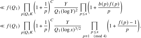 $$\begin{align*}\begin{aligned} &\ll f(Q_1) \prod_{p|Q_1K}\left(1+\frac{1}{p} \right)^C \frac{Y}{Q_1 (\log Y)^2} \prod_{p \le x} \left(1+\frac{b(p)f(p)}{p} \right) \\ &\ll f(Q_1) \prod_{p|Q_1K}\left(1+\frac{1}{p} \right)^C \frac{Y}{Q_1 (\log x)^{3/2}} \prod_{\substack{p \le x \\ p \equiv 1\ \ \ {\pmod 4}}} \left(1+\frac{f(p)-1}{p} \right). \end{aligned} \end{align*}$$
Hence, the claim follows in the same way as before.
Lemma 4.3. Let $(\log \log x)^4 \le U \le \frac {1}{10}(\log x)^{1/2}$
. There exists
$(\log \log x)^4 \le U \le \frac {1}{10}(\log x)^{1/2}$
. There exists $C>0$
such that for all
$C>0$
such that for all $n \in {\mathcal N}_j(x)$
,
$n \in {\mathcal N}_j(x)$
, $j=1,2$
, outside a set of size
$j=1,2$
, outside a set of size
 $$ \begin{align*}\ll \frac{1}{\varepsilon^2} \cdot \# {\mathcal N}_j(x) \prod_{p|Q_1Q_0}\left( 1+\frac{1}{p}\right)^C \frac{(\log \log x)^4}{U}\end{align*} $$
the following hold:
 $$ \begin{align} \sum_{\substack{1 \le |k| \le \frac{1}{U}(\log x)^{1/2} \\ k \neq 4}} b(Q_0n+k)=0, \end{align} $$
 $$ \begin{align} \sum_{\substack{ 1 \le |k| \le \frac{n}{2x}(\log x)^{B} \\ k \neq 4}} \frac{r(Q_0n+k)}{|k|} \le U \end{align} $$
and
 $$ \begin{align} \sum_{ |k| \ge U } \frac{r(Q_0n+k)}{k^2} \le \frac{1}{\log \log x}. \end{align} $$
Proof. We first establish equation (4.7). By Chebyshev’s inequality
 $$ \begin{align} \# \bigg\{ n \in {\mathcal N}_j(x) : \sum_{\substack{1 \le |k| \le \frac{1}{U}(\log x)^{1/2} \\ k \neq 4}} b(Q_0n+k) \ge 1 \bigg\} \le \sum_{\substack{1 \le |k| \le \frac{1}{U}(\log x)^{1/2} \\ k \neq 4}} \sum_{n \in {\mathcal N}_j(x)} b(Q_0n+k). \end{align} $$
Applying Lemma 4.2 to the inner sum and noting that
 $$\begin{align*}\prod_{p \le x} \left(1+\frac{b(p)-1}{p} \right)\ll \frac{1}{\sqrt{\log x}},\\[-7pt] \end{align*}$$
we get that the LHS of equation (4.10) is bounded by
 $$ \begin{align} \begin{aligned} &\ll\prod_{p |Q_1Q_0} \left(1+\frac{1}{p} \right)^C \frac{\# {\mathcal N}_j(x)}{\varepsilon^2 \sqrt{\log x}} \sum_{\substack{1 \le |k| \le \frac{1}{U}(\log x)^{1/2} \\ k \neq 4}} g(k)\\ &\ll \prod_{p |Q_1Q_0} \left(1+\frac{1}{p} \right)^C \frac{\# {\mathcal N}_j(x)}{\varepsilon^2} \frac{(\log \log x)^2}{U}, \end{aligned}\\[-7pt]\nonumber \end{align} $$
where the second step follows upon using Lemma 4.1.
To prove equation (4.8), we argue similarly and apply Lemmas 4.1 and 4.2 to get
 $$ \begin{align*} \begin{aligned} &\# \bigg\{ n \in {\mathcal N}_j(x) : \sum_{\substack{ 1 \le |k| \le \frac{n}{2x}(\log x)^{B} \\ k \neq 4}} \frac{r(Q_0n+k)}{|k|}> U \bigg\} \\ & \qquad \qquad \qquad \le \frac{1}{U} \sum_{\substack{ 1 \le |k| \le (\log x)^{B} \\ k \neq 4}} \frac{1}{|k|}\sum_{n \in {\mathcal N}_j(x)} r(Q_0n+k) \\ & \qquad \qquad \qquad \ll \frac{\# {\mathcal N}_j(x)}{\varepsilon^2 U} \prod_{p|Q_0Q_1}\left(1+\frac{1}{p} \right)^C \sum_{\substack{ 1 \le |k| \le (\log x)^{B} \\ k \neq 4}} \frac{g(k)}{|k|} \\ & \qquad \qquad \qquad \ll \frac{\# {\mathcal N}_j(x)}{\varepsilon^2 U} \prod_{p|Q_0Q_1}\left(1+\frac{1}{p} \right)^C (\log \log x)^3. \end{aligned}\\[-7pt] \end{align*} $$
We will omit the proof of equation (4.9) since it follows similarly.
For almost all $n \in {\mathcal N}_1(x)$
, it is possible to show that
$n \in {\mathcal N}_1(x)$
, it is possible to show that $r(Q_0n+4) \asymp (\log n)^{\log 2/2\pm o(1)}$
; however, since we do not actually need this estimate we will record the weaker estimate below, which suffices for our purposes and is simpler to prove.
$r(Q_0n+4) \asymp (\log n)^{\log 2/2\pm o(1)}$
; however, since we do not actually need this estimate we will record the weaker estimate below, which suffices for our purposes and is simpler to prove.
Lemma 4.4. Let $\nu>0$
be sufficiently small. There exists
$\nu>0$
be sufficiently small. There exists $C>0$
such that for all
$C>0$
such that for all $n \in {\mathcal N}_1(x)$
outside a set of size
$n \in {\mathcal N}_1(x)$
outside a set of size
 $$ \begin{align*}\ll \frac{r(Q_1)}{\varepsilon^2} \# {\mathcal N}_1(x) \frac{(\log \log x)^C}{(\log x)^{\nu}}\\[-7pt]\end{align*} $$
the following holds
 $$ \begin{align} (\log x)^{1/4-\nu} \le r(Q_0n+4) \le (\log x)^{1/2+\nu}. \end{align} $$
Proof. We begin with proving the lower bound stated in equation (4.12). Let $\omega _1(n)=\sum _{\substack {p |n \\ p \equiv 1\ \pmod 4}} 1$
. For n which is a sum of two squares
$\omega _1(n)=\sum _{\substack {p |n \\ p \equiv 1\ \pmod 4}} 1$
. For n which is a sum of two squares $r(n) \ge 2^{\omega _1(n)}$
. Using this with Chebyshev’s inequality and Lemma 4.2, the number of
$r(n) \ge 2^{\omega _1(n)}$
. Using this with Chebyshev’s inequality and Lemma 4.2, the number of $n \in {\mathcal N}_1(x)$
which
$n \in {\mathcal N}_1(x)$
which $r(Q_0n+4)<(\log x)^{1/4-\nu }$
is bounded by
$r(Q_0n+4)<(\log x)^{1/4-\nu }$
is bounded by
 $$\begin{align*}\begin{aligned} (\log x)^{1/4-\nu}\sum_{n \in {\mathcal N}_1(x)} 2^{-\omega_1(Q_0n+4)} \ll & (\log x)^{1/4-\nu} \cdot \frac{(\log \log x)^C}{\sqrt{\log x}} \prod_{\substack{p \le x \\ p \equiv 1\ \ \ {\pmod 4}}}\left(1+\frac{1}{2p} \right) \cdot \frac{1}{\varepsilon^2} \# {\mathcal N}_1(x) \\ \ll & \frac{1}{\varepsilon^2} \# {\mathcal N}_1(x) \frac{(\log \log x)^C}{(\log x)^{\nu}} \end{aligned} \end{align*}$$
using Lemma 4.2.
The proof of the upper bound is similar: The number of $n \in {\mathcal N}_1(x)$
for which
$n \in {\mathcal N}_1(x)$
for which $r(Q_0n+4)> (\log x)^{1/2+\nu }$
is, again by using Lemma 4.2, bounded by
$r(Q_0n+4)> (\log x)^{1/2+\nu }$
is, again by using Lemma 4.2, bounded by
 $$\begin{align*}\begin{aligned} \frac{1}{(\log x)^{1/2+\nu}} \sum_{n \in {\mathcal N}_1(x)} r(Q_0n+4) & \ll \frac{r(Q_1)(\log \log x)^{C} \cdot \# {\mathcal N}_1(x)}{ \varepsilon^{2} \cdot (\log x)^{1/2+\nu}} \prod_{\substack{p \le x \\ p \equiv 1\ \ \ {\pmod 4}}} \left( 1 + \frac{r(p)-1}{p}\right)\\ & \ll \frac{r(Q_1)(\log \log x)^{C}}{ \varepsilon^{2} \cdot(\log x)^{\nu}} \# {\mathcal N}_1(x). \end{aligned} \\[-44pt]\end{align*}$$
Proof of Proposition 4.1
By Theorem 3.1, for say $A=3$
, we get for all but
$A=3$
, we get for all but $O(x/(\log x)^A)$
new eigenvalues
$O(x/(\log x)^A)$
new eigenvalues $ \lambda _{\ell } \le 2x$
that
$ \lambda _{\ell } \le 2x$
that
 $$\begin{align*}\sum_{|m-\ell| \le \frac{\ell}{2x}(\log x)^B} \frac{r(m)}{m-\lambda_{\ell}}=\begin{cases} \pi \log \lambda_{\ell}+O(1) & \text{in the weak coupling quantization},\\ \frac{1}{\alpha}+O\left(1 \right) & \text{in the strong coupling quantization}. \end{cases} \end{align*}$$
We now consider integers $\ell =Q_0n$
with
$\ell =Q_0n$
with $n \in {\mathcal N}_j(x)$
,
$n \in {\mathcal N}_j(x)$
, $j=1,2$
such that the above holds. Writing
$j=1,2$
such that the above holds. Writing $m = \ell + k$
and using Lemma 4.3 with
$m = \ell + k$
and using Lemma 4.3 with $U=(\log \log x)^5$
, we find, by equation (4.7), that
$U=(\log \log x)^5$
, we find, by equation (4.7), that $r(\ell +k)/(\ell +k-\lambda _{l})=0$
for
$r(\ell +k)/(\ell +k-\lambda _{l})=0$
for $k \le (\log x)^{1/2}/U$
unless
$k \le (\log x)^{1/2}/U$
unless $k=0,4$
. Further, for
$k=0,4$
. Further, for $k \ge (\log x)^{1/2}/U$
, we have
$k \ge (\log x)^{1/2}/U$
, we have $|r(\ell +k)/(\ell +k-\lambda _{l})| \ll r(\ell +k)/k$
, and it follows (cf. equation (4.8)) that for all but
$|r(\ell +k)/(\ell +k-\lambda _{l})| \ll r(\ell +k)/k$
, and it follows (cf. equation (4.8)) that for all but $O(\# {\mathcal N}_j/(\varepsilon ^2(\log \log x)^{1-o(1)}))$
of these integers
$O(\# {\mathcal N}_j/(\varepsilon ^2(\log \log x)^{1-o(1)}))$
of these integers $n \in {\mathcal N}_j(x)$
,
$n \in {\mathcal N}_j(x)$
, $j=1,2$
, with
$j=1,2$
, with $\ell =Q_0n$
that
$\ell =Q_0n$
that $\ell ^+=\ell +4$
and
$\ell ^+=\ell +4$
and
 $$\begin{align*}\begin{aligned} \sum_{|m-\ell| \le \frac{\ell }{x}(\log x)^B} \frac{r(m)}{m-\lambda_{\ell}}=\frac{r(\ell)}{\ell-\lambda_{\ell}}+\frac{r(\ell^+)}{\ell^+-\lambda_{\ell}}+O\left((\log \log x)^5 \right). \end{aligned} \end{align*}$$
Combining the two estimates above completes the proof.
5 Proofs of the main theorems
5.1 Quantization of observables
On the unit cotangent bundle ${\mathbb S}^* M \mathbb \cong \mathbb T^2\times S^1$
, a smooth function
${\mathbb S}^* M \mathbb \cong \mathbb T^2\times S^1$
, a smooth function $f \in C^{\infty }(T^2\times S^1)$
has the Fourier expansion
$f \in C^{\infty }(T^2\times S^1)$
has the Fourier expansion
 $$\begin{align*}f(x, e^{i\phi}) =\sum_{ \zeta \in \mathbb Z^2, k \in \mathbb Z} \widehat f(\zeta,k) e^{i \langle x, \zeta \rangle +i k \phi}. \end{align*}$$
Following Kurlberg and Ueberschär [Reference Kurlberg and Ueberschär27], we quantize our observables as follows. For $g \in L^2(\mathbb T^2)$
, let
$g \in L^2(\mathbb T^2)$
, let
 $$ \begin{align} (\operatorname{Op}(f) g)(x)=\sum_{ \xi \in \mathbb Z^2 \setminus 0 }\sum_{ \zeta \in \mathbb Z^2 , k \in \mathbb Z} \widehat f(\zeta,k) e^{ik \arg \xi} \widehat g(\xi) e^{i \langle \zeta+\xi, x \rangle}+\sum_{ \zeta \in \mathbb Z^2 , k \in \mathbb Z} \widehat f(\zeta,k) \widehat g(0) e^{i \langle \zeta, x \rangle}. \end{align} $$
Hence, for pure momentum observables $f : S^1 \rightarrow \mathbb R$
, one has
$f : S^1 \rightarrow \mathbb R$
, one has
 $$ \begin{align} (\operatorname{Op}(f)g)(x)=\sum_{\xi \in \mathbb Z^2 } f\left( \frac{\xi}{|\xi|} \right) \widehat g(\xi) e^{i \langle \xi, x\rangle}, \end{align} $$
where for $\xi =0$
,
$\xi =0$
, $f(\tfrac {\xi }{|\xi |})$
is defined to be
$f(\tfrac {\xi }{|\xi |})$
is defined to be $f(1)$
. (Another option is defining it as the average
$f(1)$
. (Another option is defining it as the average $\int _{S^1} f(\theta ) \, \frac {d\theta }{2\pi }$
; a technical point is that some choice must be made to extend f to a smooth observable on the cotangent bundle; for example, see [Reference Yesha50, Section 3]. However, this choice only affects the matrix coefficients in equation (5.3) by
$\int _{S^1} f(\theta ) \, \frac {d\theta }{2\pi }$
; a technical point is that some choice must be made to extend f to a smooth observable on the cotangent bundle; for example, see [Reference Yesha50, Section 3]. However, this choice only affects the matrix coefficients in equation (5.3) by $O(1/(\lVert G_{\lambda } \rVert _2 \cdot \lambda ^{2})$
.)
$O(1/(\lVert G_{\lambda } \rVert _2 \cdot \lambda ^{2})$
.)
Let $g_{\lambda }$
be as given in equation (1.4). Then for f a pure momentum observable it follows from equations (1.4) and (5.2) that
$g_{\lambda }$
be as given in equation (1.4). Then for f a pure momentum observable it follows from equations (1.4) and (5.2) that
 $$ \begin{align} \begin{aligned} \langle \operatorname{Op}(f) g_{\lambda}, g_{\lambda} \rangle =& \frac{1}{16 \pi^4 }\cdot \frac{1}{\lVert G_{\lambda} \rVert_2^2} \sum_{ n \ge 0 }\frac{1}{(n-\lambda)^2} \sum_{ a^2+b^2=n} f\left(\frac{a+ib}{|a+ib|} \right) \\ =&\frac{1}{\sum_{n \ge 0} \frac{r(n)}{(n-\lambda)^2}} \sum_{ n \ge 0 }\frac{1}{(n-\lambda)^2} \sum_{ a^2+b^2=n} f\left(\frac{a+ib}{|a+ib|} \right). \end{aligned} \end{align} $$
5.2 Measures associated to sequences of almost primes in narrow sectors
Let ${\mathcal N}_1, {\mathcal N}_2$
be as in equation (4.1). Before proceeding to the main result of this section, we will specify our choice of
${\mathcal N}_1, {\mathcal N}_2$
be as in equation (4.1). Before proceeding to the main result of this section, we will specify our choice of $Q_0,Q_1$
. Consider the set of primes
$Q_0,Q_1$
. Consider the set of primes
 $$ \begin{align} {\mathcal S}= \{ p : p=a^2+b^2, 0 \le b \le a \text{ and } \, 0 < \arctan(b/a) \le p^{-1/10} \}, \end{align} $$
and let $q_j$
be the
$q_j$
be the $jth$
element of
$jth$
element of ${\mathcal S}$
. It follows from work of Ricci [Reference Ricci35, Th’m 2, p. 21–22] that
${\mathcal S}$
. It follows from work of Ricci [Reference Ricci35, Th’m 2, p. 21–22] that
 $$\begin{align*}\# \{ p \le x : p \in {\mathcal S}\} \asymp \frac{x^{9/10}}{\log x}, \end{align*}$$
so $q_j \asymp (j \log j)^{10/9}$
. Let
$q_j \asymp (j \log j)^{10/9}$
. Let $ T = \lfloor \log \log x \rfloor $
,
$ T = \lfloor \log \log x \rfloor $
, $H= \lfloor 100 \log \log \log x\rfloor $
and
$H= \lfloor 100 \log \log \log x\rfloor $
and
 $$ \begin{align} Q_0'= \prod_{j=T}^{T+H-1} q_j, \qquad Q_1'=\prod_{j=T+H}^{T+2H-1} q_j. \end{align} $$
Also, let $r_0, r_1 \in {\mathcal S}$
with
$r_0, r_1 \in {\mathcal S}$
with $\tfrac 14 \log \log x \le r_0,r_1 \le \frac 12 \log \log x$
and
$\tfrac 14 \log \log x \le r_0,r_1 \le \frac 12 \log \log x$
and $a_0,a_1 \in \mathbb Z$
with
$a_0,a_1 \in \mathbb Z$
with $0 \le a_0,a_1 \le \log \log \log x$
. Let
$0 \le a_0,a_1 \le \log \log \log x$
. Let $m_0,m_1$
be integers, which are fixed (in terms of x), whose prime factors are all congruent to
$m_0,m_1$
be integers, which are fixed (in terms of x), whose prime factors are all congruent to $1\ \pmod 4$
. Write
$1\ \pmod 4$
. Write $(m_0,m_1)=p_1^{e_1}\cdots p_s^{e_s}$
, and let
$(m_0,m_1)=p_1^{e_1}\cdots p_s^{e_s}$
, and let $g'=\widetilde p_1^{e_1} \cdots \widetilde p_s^{e_s}$
, where
$g'=\widetilde p_1^{e_1} \cdots \widetilde p_s^{e_s}$
, where $\tfrac 12 \log \log x < \widetilde p_j < \log \log x$
,
$\tfrac 12 \log \log x < \widetilde p_j < \log \log x$
, $\widetilde p_j=c_j^2+d_j^2$
with
$\widetilde p_j=c_j^2+d_j^2$
with $0 \le c_j \le d_j$
and
$0 \le c_j \le d_j$
and $\arctan (c_j/d_j)=\arctan (b_j/a_j)+O(1/(\log \log x)^{1/10})$
, where
$\arctan (c_j/d_j)=\arctan (b_j/a_j)+O(1/(\log \log x)^{1/10})$
, where $a_j^2+b_j^2=p_j$
with
$a_j^2+b_j^2=p_j$
with $0 \le b_j \le a_j$
, for each
$0 \le b_j \le a_j$
, for each $j=1, \ldots , s$
. (Note that such primes exist by Ricci’s result on angular equidistribution of Gaussian primes.) We now take
$j=1, \ldots , s$
. (Note that such primes exist by Ricci’s result on angular equidistribution of Gaussian primes.) We now take
 $$ \begin{align} Q_0=Q_0'm_0 r_0^{a_0}, \qquad Q_1=Q_1' \frac{m_1}{(m_0,m_1)} r_1^{a_1}g'. \end{align} $$
Note that $(Q_0,Q_1)=1$
and that
$(Q_0,Q_1)=1$
and that $Q_0,Q_1 \ll \exp (200 (\log \log \log x)^2) \le (\log x)^{1/10}$
so that this choice of
$Q_0,Q_1 \ll \exp (200 (\log \log \log x)^2) \le (\log x)^{1/10}$
so that this choice of $Q_0,Q_1$
is consistent with our prior assumption. For
$Q_0,Q_1$
is consistent with our prior assumption. For $j=1,2$
, let
$j=1,2$
, let
 $$ \begin{align} \mathcal M_{j}(x)=\{ x \le m \le 2 x : m=Q_0n \text{ and } n \in {\mathcal N}_{j}\}. \end{align} $$
It follows from equation (4.3) that
 $$ \begin{align} \# \mathcal M_1(x) \asymp \varepsilon^2 \frac{1}{\varphi(Q_1)} \frac{x \log \log x}{Q_0(\log x)^{3/2}}\\[-10pt]\nonumber \end{align} $$
and
 $$ \begin{align} \# \mathcal M_2(x) \asymp \varepsilon^2 \frac{1}{\varphi(Q_0Q_1)} \frac{x \log \log x}{(\log x)^{2}}.\\[-10pt]\nonumber \end{align} $$
Recall that we have chosen
 $$\begin{align*}\varepsilon = (\log \log x)^{-1/11}.\\[-10pt] \end{align*}$$
Lemma 5.1. Let $Q_0,Q_1$
be as in equation (5.6) and
$Q_0,Q_1$
be as in equation (5.6) and $ \eta>0$
be as in Proposition 2.1. Let
$ \eta>0$
be as in Proposition 2.1. Let $m \in \mathcal M_j(x)$
,
$m \in \mathcal M_j(x)$
, $j=1,2$
, where
$j=1,2$
, where $\mathcal M_j(x)$
is defined as in equation (5.7). Then for
$\mathcal M_j(x)$
is defined as in equation (5.7). Then for $f\in C^1(S^1)$
with
$f\in C^1(S^1)$
with $|f'| \ll 1$
 $$ \begin{align} \frac{1}{r(m)} \sum_{a^2+b^2=m}f\left(\frac{a+ib}{|a+ib|} \right) =\frac{1}{r(m_0)} \sum_{a^2+b^2=m_0}f\left(\frac{a+ib}{|a+ib|} \right)+O\left( \varepsilon \right).\\[-9pt]\nonumber \end{align} $$
Under the same hypotheses, we have for $m=Q_0n \in {\mathcal N}_2(x) $
that there exists an integer
$m=Q_0n \in {\mathcal N}_2(x) $
that there exists an integer $\ell _n$
which is a sum of two squares with
$\ell _n$
which is a sum of two squares with $\#\{ p|\ell _n \} \le 2/\eta $
such that
$\#\{ p|\ell _n \} \le 2/\eta $
such that
 $$ \begin{align} \frac{1}{r(m^+)} \sum_{a^2+b^2=m^+}f\left(\frac{a+ib}{|a+ib|} \right) =\frac{1}{r(m_1 \ell_n)} \sum_{a^2+b^2=m_1\ell_n}f\left(\frac{a+ib}{|a+ib|} \right)+O\left( \varepsilon \right). \end{align} $$
Proof. First, note that, for a unit, u of $\mathbb Z[i]$
, that is,
$\mathbb Z[i]$
, that is, $u \in \{\pm 1, \pm i\}$
, for any
$u \in \{\pm 1, \pm i\}$
, for any $n \in \mathbb N$
 $$ \begin{align} \sum_{a^2+b^2=n}f\left(\frac{u(a+ib)}{|a+ib|} \right)=\sum_{a^2+b^2=n}f\left(\frac{a+ib}{|a+ib|} \right). \end{align} $$
For $m \in \mathcal M_j(x)$
with
$m \in \mathcal M_j(x)$
with $j=1$
or
$j=1$
or $j=2$
, write
$j=2$
, write $m=Q_0'm_0r_0^{a_0}n$
, where
$m=Q_0'm_0r_0^{a_0}n$
, where $n \in {\mathcal N}_j(x)$
. The factorizations of the ideals
$n \in {\mathcal N}_j(x)$
. The factorizations of the ideals $(m)=((a+ib)(a-ib))$
in
$(m)=((a+ib)(a-ib))$
in $\mathbb Z[i]$
are in one-to-one correspondence with factorizations
$\mathbb Z[i]$
are in one-to-one correspondence with factorizations $(Q_0')=((c+id)(c-id))$
,
$(Q_0')=((c+id)(c-id))$
, $(m_0)=((e+if)(e-if))$
,
$(m_0)=((e+if)(e-if))$
, $(r_0^{a_0})=((g+ih)(g-ih))$
and
$(r_0^{a_0})=((g+ih)(g-ih))$
and $(n)=((k+il)(k-il))$
since
$(n)=((k+il)(k-il))$
since $Q_0',m_0,n$
are pairwise coprime. Hence, it follows from this and equation (5.12) that
$Q_0',m_0,n$
are pairwise coprime. Hence, it follows from this and equation (5.12) that
 $$ \begin{align} \frac{1}{r(m)}\sum_{a^2+b^2=m} f\left( \frac{a+ib}{|a+ib|}\right) = \frac{1}{r(Q_0')r(m_0)r(r_0^{a_0})r(n)}\sum_{\substack{\alpha \in \mathbb Z[i] \\ \alpha \overline{\alpha}=Q_0'}} \sum_{\substack{ \beta \in \mathbb Z[i] \\ \beta \overline{\beta}=m_0 } } \sum_{\substack{ \gamma \in \mathbb Z[i] \\ \gamma \overline{\gamma}=r_0^{a_0} } } \sum_{\substack{ \delta \in \mathbb Z[i] \\ \delta \overline{\delta}=n } } f\left(\frac{\alpha \beta \gamma \delta}{|\alpha \beta \gamma \delta|} \right). \end{align} $$
Let ${\mathcal S}$
be as in equation (5.4), and write the jth element of
${\mathcal S}$
be as in equation (5.4), and write the jth element of ${\mathcal S}$
as
${\mathcal S}$
as $q_j=a_j^2+b_j^2$
, with
$q_j=a_j^2+b_j^2$
, with $0 \le b_{j} \le a_{j}$
. By construction, for
$0 \le b_{j} \le a_{j}$
. By construction, for $\alpha \in \mathbb Z[i]$
with
$\alpha \in \mathbb Z[i]$
with $\alpha \overline \alpha =Q_0'$
we can write
$\alpha \overline \alpha =Q_0'$
we can write $\alpha =u \prod _{j \in J} (a_j+\epsilon _jib_j)$
where
$\alpha =u \prod _{j \in J} (a_j+\epsilon _jib_j)$
where $J = \{ T, T+1, \ldots , T+H_1-1\}$
,
$J = \{ T, T+1, \ldots , T+H_1-1\}$
, $\epsilon _j\in \{ \pm 1\}$
and u is a unit. It follows that
$\epsilon _j\in \{ \pm 1\}$
and u is a unit. It follows that
 $$\begin{align*}\begin{aligned} \frac{\alpha}{|\alpha|}& = u\prod_{j \in J}\frac{a_j+\epsilon_jib_j}{|a_j+ib_j|}\\ &= u\left(1+O\left( \sum_{j \in J } |\arctan(b_j/a_j)| \right)\right) =u+O\left( \frac{1}{(\log \log x)^{1/11}}\right), \end{aligned} \end{align*}$$
where the unit u depends on $\alpha $
. Also, for
$\alpha $
. Also, for $\gamma \in \mathbb Z[i]$
with
$\gamma \in \mathbb Z[i]$
with $\gamma \overline \gamma =r_0^{a_0}$
, we have
$\gamma \overline \gamma =r_0^{a_0}$
, we have $ \frac {\gamma }{|\gamma |}=u+O(1/(\log \log x)^{1/11}), $
and for
$ \frac {\gamma }{|\gamma |}=u+O(1/(\log \log x)^{1/11}), $
and for $\delta \in \mathbb Z[i]$
with
$\delta \in \mathbb Z[i]$
with $\delta \overline \delta =n$
, we have
$\delta \overline \delta =n$
, we have $ \frac {\delta }{|\delta |}=u+O(\varepsilon ). $
Hence, by this and equation (5.12)
$ \frac {\delta }{|\delta |}=u+O(\varepsilon ). $
Hence, by this and equation (5.12)
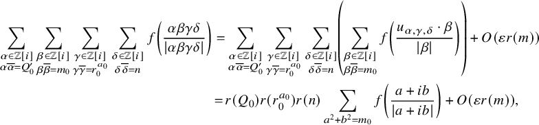 $$\begin{align*}\begin{aligned} \sum_{\substack{\alpha \in \mathbb Z[i] \\ \alpha \overline{\alpha}=Q_0'}} \sum_{\substack{ \beta \in \mathbb Z[i] \\ \beta \overline{\beta}=m_0 } } \sum_{\substack{ \gamma \in \mathbb Z[i] \\ \gamma \overline{\gamma}=r_0^{a_0} } } \sum_{\substack{ \delta \in \mathbb Z[i] \\ \delta \overline{\delta}=n } } f\left(\frac{\alpha \beta \gamma \delta}{|\alpha \beta \gamma \delta|} \right)=& \sum_{\substack{\alpha \in \mathbb Z[i] \\ \alpha \overline{\alpha}=Q_0'}} \sum_{\substack{ \gamma \in \mathbb Z[i] \\ \gamma \overline{\gamma}=r_0^{a_0} } } \sum_{\substack{ \delta \in \mathbb Z[i] \\ \delta \overline{\delta}=n } } \left( \sum_{\substack{ \beta \in \mathbb Z[i] \\ \beta \overline{\beta}=m_0 } } f\left(\frac{u_{\alpha, \gamma,\delta} \cdot \beta }{| \beta |} \right) \right)+O(\varepsilon r(m)) \\ =\,&r(Q_0) r(r_0^{a_0})r(n) \sum_{ a^2+b^2=m_0} f\left(\frac{ a+ib}{| a+ib|}\right)+O(\varepsilon r(m)), \end{aligned} \end{align*}$$
thereby proving equation (5.10).
The proof of equation (5.11) follows along the same lines upon noting that for $m=Q_0n \in \mathcal M_2(x)$
we can write
$m=Q_0n \in \mathcal M_2(x)$
we can write $m^+=Q_1' r_1^{a_1} \frac {m_1}{(m_1,m_0)} g' \ell _n$
, where
$m^+=Q_1' r_1^{a_1} \frac {m_1}{(m_1,m_0)} g' \ell _n$
, where $\ell _n$
is a sum of two squares. Note that
$\ell _n$
is a sum of two squares. Note that $Q_1',\frac {m_1}{(m_1,m_0)}, r_1^{a_1}, g',\ell _n$
are pairwise coprime by construction since all the prime divisors of
$Q_1',\frac {m_1}{(m_1,m_0)}, r_1^{a_1}, g',\ell _n$
are pairwise coprime by construction since all the prime divisors of $\ell _n$
are
$\ell _n$
are $\ge y$
; the latter also implies that
$\ge y$
; the latter also implies that $\#\{ p|\ell _n \} \le 2/\eta $
. Also, note that since all primes dividing
$\#\{ p|\ell _n \} \le 2/\eta $
. Also, note that since all primes dividing $g', Q_{1}', r_{1}$
have very small Gaussian angles (by construction), the set of Gaussian angles associated with
$g', Q_{1}', r_{1}$
have very small Gaussian angles (by construction), the set of Gaussian angles associated with $m^{+}$
is very close to the set of angles associated with
$m^{+}$
is very close to the set of angles associated with $m_{1} \ell _{n}$
, after taking multiplicities into account.
$m_{1} \ell _{n}$
, after taking multiplicities into account.
5.3 Proof of Theorem 1.1
Since Gaussian angles associated with inert primes are trivial, we can without loss of generality assume all the prime factors of $m_0$
are congruent to
$m_0$
are congruent to $1\ \pmod 4$
. Let
$1\ \pmod 4$
. Let $Q_0,Q_1$
be as in equation (5.6) and
$Q_0,Q_1$
be as in equation (5.6) and $\mathcal M_1(x)$
be as in equation (5.7), and recall for
$\mathcal M_1(x)$
be as in equation (5.7), and recall for $m \in \mathcal M_1(x)$
that
$m \in \mathcal M_1(x)$
that $m=Q_0n$
, where
$m=Q_0n$
, where $n \in {\mathcal N}_1(x)$
and
$n \in {\mathcal N}_1(x)$
and ${\mathcal N}_1$
is as in equation (4.1). By equation (4.7) and Lemma 4.4 it follows that for all but at most
${\mathcal N}_1$
is as in equation (4.1). By equation (4.7) and Lemma 4.4 it follows that for all but at most $o(\# \mathcal M_1(x))$
integers
$o(\# \mathcal M_1(x))$
integers $m \in \mathcal M_1(x)$
that
$m \in \mathcal M_1(x)$
that $m^+=m+4$
,
$m^+=m+4$
, $(\log x)^{1/4-\nu } \le r(m^+) \le (\log x)^{1/2+\nu }$
(for any fixed
$(\log x)^{1/4-\nu } \le r(m^+) \le (\log x)^{1/2+\nu }$
(for any fixed $\nu>0$
) and
$\nu>0$
) and $4 \le r(m) \ll (\log x)^{o(1)}$
. Combining this with Proposition 4.1, we get that for all but
$4 \le r(m) \ll (\log x)^{o(1)}$
. Combining this with Proposition 4.1, we get that for all but $o(\# \mathcal M_1(x))$
integers
$o(\# \mathcal M_1(x))$
integers $m \in \mathcal M_1(x)$
that
$m \in \mathcal M_1(x)$
that $\lambda _m-m=o(1)$
and moreover
$\lambda _m-m=o(1)$
and moreover
 $$ \begin{align} \lambda_m-m \asymp \begin{cases} \displaystyle \frac{r(m)}{\log \lambda_m} & \text{ in the weak coupling quantization},\\[10pt] \displaystyle \frac{r(m)}{r(m^+)} & \text{ in the strong coupling quantization}. \end{cases} \end{align} $$
Also, note that, for such m as above, we also have $|\lambda _m-m^+| \ge 3$
. Hence, using the above estimate along with equations (4.7) and (4.9) with
$|\lambda _m-m^+| \ge 3$
. Hence, using the above estimate along with equations (4.7) and (4.9) with $U= (\log \log x)^5$
we get for all but at most
$U= (\log \log x)^5$
we get for all but at most $o(\# \mathcal M_1(x))$
integers
$o(\# \mathcal M_1(x))$
integers $m \in \mathcal M_1(x)$
that (in both cases)
$m \in \mathcal M_1(x)$
that (in both cases)
 $$ \begin{align} \begin{aligned} \sum_{\ell \ge 0} \frac{r(\ell)}{(\ell-\lambda_m)^2} =&\frac{r(m)}{(m-\lambda_m)^2}+\frac{r(m^+)}{(m^+-\lambda_m)^2}+o(1) \\ =&\frac{r(m)}{(m-\lambda_m)^2}\left(1+O\left( \frac{r(m^+)(m-\lambda_m)^2}{r(m)} \right) \right)+o(1)\\ =&\frac{r(m)}{(m-\lambda_m)^2}\left(1+o(1) \right). \end{aligned} \end{align} $$
Similarly, for all but at most $o(\# \mathcal M_1(x))$
integers
$o(\# \mathcal M_1(x))$
integers $m \in \mathcal M_1(x)$
 $$ \begin{align} \sum_{ \ell \ge 0 }\frac{1}{(\ell-\lambda_m)^2} \sum_{ a^2+b^2=\ell} f\left(\frac{a+ib}{|a+ib|} \right)= \frac{1}{(m-\lambda_m)^2}\sum_{ a^2+b^2=m} f\left(\frac{a+ib}{|a+ib|} \right)+O(r(m^+)). \end{align} $$
Therefore, combining equations (5.3), (5.14), (5.15) and (5.16), it follows for all but at most $o(\# \mathcal M_1(x))$
integers
$o(\# \mathcal M_1(x))$
integers $m \in \mathcal M_1(x)$
we have that
$m \in \mathcal M_1(x)$
we have that
 $$\begin{align*}\begin{aligned} \langle \operatorname{Op}(f) g_{\lambda_m}, g_{\lambda_m} \rangle=& (1+o(1)) \frac{(m-\lambda_m)^2}{r(m)} \cdot \left( \frac{1}{(m-\lambda_m)^2}\sum_{ a^2+b^2=m} f\left(\frac{a+ib}{|a+ib|} \right)+O(r(m^+))\right) \\ =&(1+o(1))\frac{1}{r(m)} \sum_{ a^2+b^2=m} f\left(\frac{a+ib}{|a+ib|} \right) +o(1)\\ =& (1+o(1)) \frac{1}{r(m_0)} \sum_{a^2+b^2=m_0} f\left(\frac{a+ib}{|a+ib|} \right)+O(\varepsilon), \end{aligned} \end{align*}$$
where the last step follows by equation (5.10). The estimate for the density of this subsequence of eigenvalues follows immediately from equation (5.8), noting that $Q_0,Q_1 \ll (\log x)^{o(1)}$
.
$Q_0,Q_1 \ll (\log x)^{o(1)}$
.
5.4 Proof of Theorem 1.2
As before, without loss of generality, we can assume all the prime factors of $m_0,m_1$
are congruent to
$m_0,m_1$
are congruent to $1\ \pmod 4$
. For the sake of brevity, let
$1\ \pmod 4$
. For the sake of brevity, let $\mathcal L_2=\log \log x$
. Let
$\mathcal L_2=\log \log x$
. Let $Q_0,Q_1$
be as in equation(5.6) and
$Q_0,Q_1$
be as in equation(5.6) and $\mathcal M_2(x)$
be as in equation (5.7), and recall for
$\mathcal M_2(x)$
be as in equation (5.7), and recall for $m \in \mathcal M_2(x)$
that
$m \in \mathcal M_2(x)$
that $m=Q_0n$
, where
$m=Q_0n$
, where $n \in {\mathcal N}_2(x)$
where
$n \in {\mathcal N}_2(x)$
where ${\mathcal N}_2$
is as in equation (4.1). Note for each
${\mathcal N}_2$
is as in equation (4.1). Note for each $m \in \mathcal M_2(x)$
that
$m \in \mathcal M_2(x)$
that $r(m) \gg \mathcal L_2^{10}$
. Also, by construction
$r(m) \gg \mathcal L_2^{10}$
. Also, by construction $r(m)/r(m+4) \asymp \frac {a_0+1}{a_1+1}$
, where
$r(m)/r(m+4) \asymp \frac {a_0+1}{a_1+1}$
, where $H,a_0,a_1$
are also as in equation (5.6), and note
$H,a_0,a_1$
are also as in equation (5.6), and note $a_0,a_1 \le \log \mathcal L_2$
. Applying Proposition 4.1, we get that for all
$a_0,a_1 \le \log \mathcal L_2$
. Applying Proposition 4.1, we get that for all $m \in \mathcal M_2(x)$
outside an exceptional set of size
$m \in \mathcal M_2(x)$
outside an exceptional set of size $o(\#\mathcal M_2(x))$
that
$o(\#\mathcal M_2(x))$
that $m^+=m+4$
and
$m^+=m+4$
and
 $$ \begin{align} \frac{\lambda_m-m}{m^+-\lambda_m}=\frac{r(m)}{r(m^+)}\left(1+O\left(\frac{\mathcal L_2^6}{r(m)}\right)\right)=\frac{r(m)}{r(m^+)}\left(1+O\left(\mathcal L_2^{-4}\right)\right). \end{align} $$
In particular, this implies that $\lambda _m-m \gg \mathcal L_2^{-1}$
and
$\lambda _m-m \gg \mathcal L_2^{-1}$
and $m^+-\lambda _m \gg \mathcal L_2^{-1}$
. As before, using equations (4.7) and (4.9) with
$m^+-\lambda _m \gg \mathcal L_2^{-1}$
. As before, using equations (4.7) and (4.9) with $U= \mathcal L_2^5$
, we get for all but at most
$U= \mathcal L_2^5$
, we get for all but at most $o(\# \mathcal M_2(x))$
integers
$o(\# \mathcal M_2(x))$
integers $m \in \mathcal M_2(x)$
that
$m \in \mathcal M_2(x)$
that
 $$ \begin{align} \begin{aligned} \sum_{\ell \ge 0} \frac{r(\ell)}{(\ell-\lambda_m)^2}=\frac{r(m)}{(m-\lambda_m)^2}+\frac{r(m^+)}{(m^+-\lambda_m)^2}+O(\mathcal L_2^{-1}) \end{aligned} \end{align} $$
and
 $$ \begin{align} \begin{aligned} \sum_{ \ell \ge 0 }\frac{1}{(\ell-\lambda_m)^2} \sum_{ a^2+b^2=\ell} f\left(\frac{a+ib}{|a+ib|} \right)=& \frac{1}{(m-\lambda_m)^2}\sum_{ a^2+b^2=m} f\left(\frac{a+ib}{|a+ib|} \right)\\ &+\frac{1}{(m^+-\lambda_n)^2}\sum_{ a^2+b^2=m^+} f\left(\frac{a+ib}{|a+ib|} \right) +O(\mathcal L_2^{-1}). \end{aligned} \end{align} $$
Let $C_m=\frac {1}{1+r(m)/r(m^+)}$
. Applying equations (5.17),(5.18) and (5.19) equation in (5.3), we get
$C_m=\frac {1}{1+r(m)/r(m^+)}$
. Applying equations (5.17),(5.18) and (5.19) equation in (5.3), we get
 $$ \begin{align} \begin{aligned} &\langle \operatorname{Op}(f) g_{\lambda_m}, g_{\lambda_m} \rangle=(1+O(\mathcal L_2^{-1})) \left(\frac{r(m)}{(m-\lambda_m)^2}+\frac{r(m^+)}{(m^+-\lambda_m)^2} \right)^{-1} \\ & \qquad \times \left( \frac{1}{(m-\lambda_m)^2}\sum_{ a^2+b^2=m} f\left(\frac{a+ib}{|a+ib|} \right) +\frac{1}{(m^+-\lambda_m)^2}\sum_{ a^2+b^2=m^+} f\left(\frac{a+ib}{|a+ib|} \right)+O(\mathcal L_2^{-1})\right) \\ &\qquad =\frac{C_m}{r(m)} \sum_{ a^2+b^2=m} f\left(\frac{a+ib}{|a+ib|} \right)+\frac{1-C_m}{r(m^+)}\sum_{ a^2+b^2=m^+} f\left(\frac{a+ib}{|a+ib|} \right)+O(\mathcal L_2^{-1}). \end{aligned} \end{align} $$
Applying equation (5.10) to the first sum above, we get
 $$ \begin{align} \frac{C_m}{r(m)} \sum_{ a^2+b^2=m} f\left(\frac{a+ib}{|a+ib|} \right)= \frac{C_m}{r(m_0)} \sum_{ a^2+b^2=m_0} f\left(\frac{a+ib}{|a+ib|} \right)+O(\varepsilon). \end{align} $$
Similarly, applying equation (5.11) to the second sum on the RHS of equation (5.20) we get that
 $$ \begin{align} \frac{1-C_m}{r(m^+)} \sum_{ a^2+b^2=m^+} f\left(\frac{a+ib}{|a+ib|} \right)= \frac{1-C_m}{r(m_1\ell_n)} \sum_{ a^2+b^2=m_1 \ell_n} f\left(\frac{a+ib}{|a+ib|} \right)+O(\mathcal L_2^{-1/11}), \end{align} $$
for some integer $\ell _n$
with
$\ell _n$
with $\#\{p: p|\ell _m\} \le 2/\eta $
by equation (4.2). Using equations (5.21) and (5.22) in equation (5.20) completes the proof upon recalling that
$\#\{p: p|\ell _m\} \le 2/\eta $
by equation (4.2). Using equations (5.21) and (5.22) in equation (5.20) completes the proof upon recalling that $\varepsilon =\mathcal L_2^{-1/11}$
. The estimate for the density of this subsequence of eigenvalues follows from equation (5.9).
$\varepsilon =\mathcal L_2^{-1/11}$
. The estimate for the density of this subsequence of eigenvalues follows from equation (5.9).
5.5 Proof of Theorem 1.3
The proof of Theorem 1.3 relies on the following hypothesis concerning the distribution of primes.
Hypothesis 1. Let $Q_1,Q_0$
be as in equation (5.6) and
$Q_1,Q_0$
be as in equation (5.6) and $ \varepsilon \ge (\log \log x)^{-1/2}$
be sufficiently small. Also, let
$ \varepsilon \ge (\log \log x)^{-1/2}$
be sufficiently small. Also, let $y=x^{\eta }$
, where
$y=x^{\eta }$
, where $\eta>0$
is sufficiently small. Then the number of solutions
$\eta>0$
is sufficiently small. Then the number of solutions $(u,v) \in \mathbb Z^2$
to
$(u,v) \in \mathbb Z^2$
to
 $$\begin{align*}Q_1u-Q_0v=4, \end{align*}$$
where $v=p_1p_2$
and
$v=p_1p_2$
and $u=p_3$
are primes satisfying
$u=p_3$
are primes satisfying $1_{\mathcal P_{\varepsilon }}(p_1)1_{{\mathcal P}_{\varepsilon }'}(p_2)1_{\mathcal P_{\varepsilon }}(p_3)=1$
,
$1_{\mathcal P_{\varepsilon }}(p_1)1_{{\mathcal P}_{\varepsilon }'}(p_2)1_{\mathcal P_{\varepsilon }}(p_3)=1$
, $p_3> y$
such that
$p_3> y$
such that $ v \le x$
is
$ v \le x$
is
 $$\begin{align*}\gg \varepsilon^3 \frac{Q_0}{\varphi(Q_0 Q_1)} \frac{x \log \log x}{(\log x)^2}, \end{align*}$$
where ${\mathcal P}_{\varepsilon }, {\mathcal P}_{\varepsilon }'$
are as in equation (2.1).
${\mathcal P}_{\varepsilon }, {\mathcal P}_{\varepsilon }'$
are as in equation (2.1).
Proof of Theorem 1.3
Recall the definition of ${\mathcal N}_2$
given in equation (4.1). Let us define
${\mathcal N}_2$
given in equation (4.1). Let us define
 $$\begin{align*}{\mathcal N}_3=\{ n \in {\mathcal N}_2 : Q_0n+4=Q_1 p , b(p)=1, \, \&\, |\theta_p| \le \varepsilon\}. \end{align*}$$
Following equation (5.7), we also define
 $$\begin{align*}\mathcal M_3(x)=\{ m \le x : m=Q_0n \text{ and } n \in {\mathcal N}_3\}.\end{align*}$$
By Hypothesis 1 and equation (5.9), it follows that
 $$ \begin{align} \# \mathcal M_3(x) \asymp \varepsilon \# \mathcal M_2(x), \end{align} $$
where we also have used an upper bound sieve to get that $\# \mathcal M_3(x) \ll \varepsilon \# \mathcal M_2(x)$
. Observe that
$\# \mathcal M_3(x) \ll \varepsilon \# \mathcal M_2(x)$
. Observe that $\mathcal M_3(x) \subset \mathcal M_2(x)$
and the exceptional set in Proposition 4.1 is
$\mathcal M_3(x) \subset \mathcal M_2(x)$
and the exceptional set in Proposition 4.1 is $o(\# \mathcal M_3(x))$
since we take
$o(\# \mathcal M_3(x))$
since we take $\varepsilon =(\log \log x)^{-1/4}$
. Hence, we get that equation (5.17) holds for
$\varepsilon =(\log \log x)^{-1/4}$
. Hence, we get that equation (5.17) holds for $m \in \mathcal M_3(x)$
outside an exceptional set of size
$m \in \mathcal M_3(x)$
outside an exceptional set of size $o(\# \mathcal M_3(x))$
. Similarly, we can conclude that equations (5.18) and (5.19) also hold for all
$o(\# \mathcal M_3(x))$
. Similarly, we can conclude that equations (5.18) and (5.19) also hold for all $m \in \mathcal M_3(x)$
outside an exceptional set of size
$m \in \mathcal M_3(x)$
outside an exceptional set of size $o(\# \mathcal M_3(x))$
. Therefore, arguing as in equations 5.20–5.22 we conclude that for
$o(\# \mathcal M_3(x))$
. Therefore, arguing as in equations 5.20–5.22 we conclude that for $m \in \mathcal M_3(x)$
outside an exceptional set of size
$m \in \mathcal M_3(x)$
outside an exceptional set of size $o(\#\mathcal M_3(x))$
we have that
$o(\#\mathcal M_3(x))$
we have that
 $$ \begin{align} \langle \operatorname{Op}(f) g_{\lambda_m}, g_{\lambda_m} \rangle =\frac{C_m}{r(m_0)} \sum_{ a^2+b^2=m_0} f\left(\frac{a+ib}{|a+ib|} \right)+ \frac{1-C_m}{r(m_1\ell_n)} \sum_{ a^2+b^2=m_1 \ell_n} f\left(\frac{a+ib}{|a+ib|} \right)+O(\mathcal L_2^{-1/11}), \end{align} $$
where $m_0,m_1$
are arbitrary, fixed integers whose prime factors are all congruent to
$m_0,m_1$
are arbitrary, fixed integers whose prime factors are all congruent to $1\ \pmod 4$
and
$1\ \pmod 4$
and $C_m=1/(1+r(m )/r(m+4))$
. By our hypothesis, we have that
$C_m=1/(1+r(m )/r(m+4))$
. By our hypothesis, we have that $\ell _n=p$
with
$\ell _n=p$
with $|\theta _p| \le \varepsilon $
and
$|\theta _p| \le \varepsilon $
and $(m_1,p)=1$
. Hence, repeating the argument used to prove equation (5.10) it follows that
$(m_1,p)=1$
. Hence, repeating the argument used to prove equation (5.10) it follows that
 $$ \begin{align} \frac{1}{r(m_1\ell_n)} \sum_{ a^2+b^2=m_1 \ell_n} f\left(\frac{a+ib}{|a+ib|} \right)=\frac{1}{r(m_1)} \sum_{ a^2+b^2=m_1 } f\left(\frac{a+ib}{|a+ib|} \right)+O(\varepsilon). \end{align} $$
Given $0 < c <1$
with
$0 < c <1$
with $c=d/e \in \mathbb Q$
, we will now specify our choice of
$c=d/e \in \mathbb Q$
, we will now specify our choice of $a_0, a_1$
(from equation (5.5)). Recall we allow
$a_0, a_1$
(from equation (5.5)). Recall we allow $a_0,a_1$
to grow slowly with x and
$a_0,a_1$
to grow slowly with x and $Q_0',Q_1'$
have the same number of prime factors. Also, by construction
$Q_0',Q_1'$
have the same number of prime factors. Also, by construction $r(\frac {m_1}{(m_0,m_1)} g')=r(m_1)$
. Let
$r(\frac {m_1}{(m_0,m_1)} g')=r(m_1)$
. Let $\mathcal L=\lfloor (\log \log \log x)^{1/2} \rfloor $
. We take
$\mathcal L=\lfloor (\log \log \log x)^{1/2} \rfloor $
. We take
 $$\begin{align*}a_0= 2(e-d) r(m_1)\mathcal L \qquad \text{ and } \qquad a_1=dr(m_0) \mathcal L.\end{align*}$$
Hence,
 $$ \begin{align} C_m=\frac{1}{1+\frac{8r(m_0)(a_0+1)}{16 r(m_1)(a_1+1)}}=\frac{d}{e}+o(1). \end{align} $$
We are now ready to complete the proof. Given any attainable measures $\mu _{\infty _0}$
,
$\mu _{\infty _0}$
, $\mu _{\infty _1}$
and
$\mu _{\infty _1}$
and $0 \le c \le 1$
, we can take
$0 \le c \le 1$
, we can take $\{m_{0,j}\}_j \ \{m_{1,j}\}$
such that
$\{m_{0,j}\}_j \ \{m_{1,j}\}$
such that $\mu _{0,j}$
weakly converges to
$\mu _{0,j}$
weakly converges to $\mu _{\infty _0}$
and
$\mu _{\infty _0}$
and $\mu _{1,j}$
weakly converges to
$\mu _{1,j}$
weakly converges to $\mu _{\infty _1}$
, as
$\mu _{\infty _1}$
, as $j \rightarrow \infty $
. We also take
$j \rightarrow \infty $
. We also take $\{a_{0,j}\}_j,\{a_{1,j}\}_j$
so that
$\{a_{0,j}\}_j,\{a_{1,j}\}_j$
so that $d_j/e_j \rightarrow c$
as
$d_j/e_j \rightarrow c$
as $j \rightarrow \infty $
. Therefore, by equations (5.24), (5.25) and (5.26) we conclude that there exists
$j \rightarrow \infty $
. Therefore, by equations (5.24), (5.25) and (5.26) we conclude that there exists $\{\lambda _{\ell }\}_{\ell } \subset \Lambda _{\text {new}}$
such that
$\{\lambda _{\ell }\}_{\ell } \subset \Lambda _{\text {new}}$
such that
 $$\begin{align*}\langle \operatorname{Op}(f) g_{\lambda_{\ell}}, g_{\lambda_{\ell}} \rangle \xrightarrow{\ell \rightarrow \infty} c\int_{S^1} f d\mu_{\infty_0} +(1-c) \int_{S^1} f d\mu_{\infty_1}.\\[-38pt] \end{align*}$$
A Arithmetic over $\mathbb Q(i)$

Consider the number field $\mathbb Q(i)$
with the corresponding ring of integers
$\mathbb Q(i)$
with the corresponding ring of integers $\mathbb Z[i]$
. For
$\mathbb Z[i]$
. For $\mathfrak b$
a nonzero integral ideal of
$\mathfrak b$
a nonzero integral ideal of $\mathbb Z[i]$
, the residue classes
$\mathbb Z[i]$
, the residue classes $\alpha\ \pmod { \mathfrak b}$
, where
$\alpha\ \pmod { \mathfrak b}$
, where $(\alpha )$
and
$(\alpha )$
and $\mathfrak b$
are relatively prime ideals, form the multiplicative group
$\mathfrak b$
are relatively prime ideals, form the multiplicative group $(\mathbb Z[i]/\mathfrak b)^*$
. We now summarize some well-known facts, which may be found in [Reference Neukirch, Schappacher and Harder34] or [Reference Iwaniec and Kowalski19]. A Dirichlet character
$(\mathbb Z[i]/\mathfrak b)^*$
. We now summarize some well-known facts, which may be found in [Reference Neukirch, Schappacher and Harder34] or [Reference Iwaniec and Kowalski19]. A Dirichlet character $\pmod {\mathfrak b}$
is a group homomorphism
$\pmod {\mathfrak b}$
is a group homomorphism
 $$\begin{align*}\chi : (\mathbb Z[i]/\mathfrak b) ^*\rightarrow S^1. \end{align*}$$
We extend $\chi $
to all of
$\chi $
to all of $\mathbb Z[i]$
by setting
$\mathbb Z[i]$
by setting $\chi (\mathfrak a)=0$
for
$\chi (\mathfrak a)=0$
for $\mathfrak a$
and
$\mathfrak a$
and $\mathfrak b$
which are not relatively prime. Let I denote multiplicative group of nonzero fractional ideals and
$\mathfrak b$
which are not relatively prime. Let I denote multiplicative group of nonzero fractional ideals and $I_{\mathfrak b}=\{\mathfrak a \in I : \mathfrak a \text { and } \mathfrak b \text { are relatively prime}\}$
. A Hecke Großencharakter
$I_{\mathfrak b}=\{\mathfrak a \in I : \mathfrak a \text { and } \mathfrak b \text { are relatively prime}\}$
. A Hecke Großencharakter $\pmod {\mathfrak b}$
is a homomorphism
$\pmod {\mathfrak b}$
is a homomorphism $\psi : I_{\mathfrak b} \rightarrow \mathbb C \setminus \{0\}$
for which there exists a pair of homomorphisms
$\psi : I_{\mathfrak b} \rightarrow \mathbb C \setminus \{0\}$
for which there exists a pair of homomorphisms
 $$\begin{align*}\chi \, : \, (\mathbb Z[i]/\mathfrak b) ^*\rightarrow S^1, \qquad \chi_{\infty} \, : \, \mathbb C^* \rightarrow S^1 \end{align*}$$
such that for an ideal $(\alpha )$
with
$(\alpha )$
with $\alpha \in \mathbb Z[i]$
 $$\begin{align*}\psi((\alpha))=\chi(\alpha)\chi_{\infty}(\alpha). \end{align*}$$
Conversely, given any $\chi\ \pmod {\mathfrak b}$
and
$\chi\ \pmod {\mathfrak b}$
and $\chi _{\infty }$
there exists a Großencharakter
$\chi _{\infty }$
there exists a Großencharakter $\psi\ \pmod {\mathfrak b}$
such that
$\psi\ \pmod {\mathfrak b}$
such that $\psi =\chi \cdot \chi _{\infty }$
provided that
$\psi =\chi \cdot \chi _{\infty }$
provided that $\chi ( u)\chi _{\infty }( u) = 1$
for each unit
$\chi ( u)\chi _{\infty }( u) = 1$
for each unit $u \in \mathbb Z[i]$
.
$u \in \mathbb Z[i]$
.
In particular, for $4|k$
and
$4|k$
and $\mathfrak a=(\alpha )$
a nonnegative integer
$\mathfrak a=(\alpha )$
a nonnegative integer
 $$\begin{align*}\psi(\mathfrak a)=\left(\frac{\alpha}{|\alpha|} \right)^{k} \end{align*}$$
is a Hecke Großenchakter $\pmod 1$
and these Hecke Großencharakteren can be used to detect primes in sectors. Additionally, given a positive rational integer q with
$\pmod 1$
and these Hecke Großencharakteren can be used to detect primes in sectors. Additionally, given a positive rational integer q with $(4,q)=1$
the homomorphism
$(4,q)=1$
the homomorphism
 $$\begin{align*}\chi \circ N : I_q \rightarrow S^1 \end{align*}$$
given by $(\chi \circ N)(\mathfrak a)=\chi (N(\mathfrak a))$
is a Dirichlet character
$(\chi \circ N)(\mathfrak a)=\chi (N(\mathfrak a))$
is a Dirichlet character $\pmod q$
, where
$\pmod q$
, where $\chi $
is a Dirichlet character
$\chi $
is a Dirichlet character $\pmod q$
for
$\pmod q$
for $\mathbb Z$
, that is
$\mathbb Z$
, that is $\chi : (\mathbb Z/(q))^* \rightarrow S^1$
, where
$\chi : (\mathbb Z/(q))^* \rightarrow S^1$
, where $N \mathfrak a$
is the norm of
$N \mathfrak a$
is the norm of $\mathfrak a$
. Hence, for
$\mathfrak a$
. Hence, for $4|k$
$4|k$
 $$\begin{align*}\psi(\mathfrak a)=(\chi \circ N)( \alpha ) \left( \frac{\alpha}{|\alpha|}\right)^k \end{align*}$$
is a Hecke Großencharakter with modulus q and frequency k, where $\mathfrak a=(\alpha )$
. (A priori
$\mathfrak a=(\alpha )$
. (A priori $\alpha $
is only defined up to multiplication by i, but for these characters the choice does not matter.) The L-function attached to the Großencharakter
$\alpha $
is only defined up to multiplication by i, but for these characters the choice does not matter.) The L-function attached to the Großencharakter $\psi $
given by
$\psi $
given by
 $$\begin{align*}L(s, \psi)=\sum_{\mathfrak a} \frac{\psi(\mathfrak a)}{N (\mathfrak a)^s} \end{align*}$$
has a functional equation and admits an analytic continuation to $\mathbb C\setminus \{1\}$
.
$\mathbb C\setminus \{1\}$
.
Moreover, if $\psi $
is not a real character,
$\psi $
is not a real character, $L(s,\psi )$
has a standard zero-free region. That is, we have
$L(s,\psi )$
has a standard zero-free region. That is, we have
 $$\begin{align*}L(\sigma+it,\psi) \neq 0 \qquad \text{ for } \qquad \sigma>1-\frac{c}{ \log (q(|t|+1)(|k|+1))} \end{align*}$$
(see [Reference Iwaniec and Kowalski19, Section 5.10]). In particular, if $k \ne 0$
,
$k \ne 0$
,
 $$\begin{align*}\sum_{N (\pi) \le x } \chi(N(\pi)) \left( \frac{\pi}{|\pi|}\right)^{k} \ll ((|k|+1) q) \cdot x \exp\left( -c \sqrt{\log x}\right), \end{align*}$$
where the summation is over prime ideal $\mathfrak p=(\pi )$
with norm
$\mathfrak p=(\pi )$
with norm $\le x$
.
$\le x$
.
Furthermore, for $k =0$
the same estimate holds for any complex
$k =0$
the same estimate holds for any complex $\chi\ \pmod q$
. However, for
$\chi\ \pmod q$
. However, for $k=0$
and
$k=0$
and $\chi\ \pmod q$
a real character, there may be a possible Siegel zero, and in this case we have Siegel’s estimate (see Section 5.9 of [Reference Iwaniec and Kowalski19])
$\chi\ \pmod q$
a real character, there may be a possible Siegel zero, and in this case we have Siegel’s estimate (see Section 5.9 of [Reference Iwaniec and Kowalski19])
 $$\begin{align*}L(\sigma+it , \chi) \neq0 \qquad \text{for } \qquad \sigma \ge 1- \frac{c(\epsilon)}{q^{\epsilon}} \end{align*}$$
for any $\epsilon>0$
. Consequently, we have the Siegel–Walfisz type prime number theorem for
$\epsilon>0$
. Consequently, we have the Siegel–Walfisz type prime number theorem for $(a,q)=1$
and
$(a,q)=1$
and $(q,2)=1$
 $$ \begin{align} \sum_{\substack{N(\pi) \le x \\ N(\pi) \equiv a\ \ \ {\pmod q} \\ 0 \le \arg \pi \le \varepsilon}} 1=\frac{1}{\varphi(q)} \sum_{\substack{N(\pi) \le x \\ (N(\pi),q)=1 \\ 0 \le \arg \pi \le \varepsilon } } 1+O\left(\frac{x}{(\log x)^A} \right) \end{align} $$
for any $A \ge 1$
. (After multiplication by
$A \ge 1$
. (After multiplication by $i^{l}$
for some l, we can ensure that
$i^{l}$
for some l, we can ensure that $\theta = \arg i^{l}\pi \in [0,\pi /2)$
; we will let
$\theta = \arg i^{l}\pi \in [0,\pi /2)$
; we will let $\arg \pi $
denote this angle.)
$\arg \pi $
denote this angle.)
Recall that a prime $p \equiv 3\ \pmod 4$
is inert in
$p \equiv 3\ \pmod 4$
is inert in $\mathbb Z[i]$
; additionally, a prime
$\mathbb Z[i]$
; additionally, a prime $p \equiv 1\ \pmod 4$
splits in
$p \equiv 1\ \pmod 4$
splits in $\mathbb Z[i]$
so that
$\mathbb Z[i]$
so that $p=\pi \overline {\pi }=a^2+b^2$
, where
$p=\pi \overline {\pi }=a^2+b^2$
, where $\pi $
is a prime in
$\pi $
is a prime in $\mathbb Z[i]$
. Writing
$\mathbb Z[i]$
. Writing
 $$\begin{align*}\mathcal B(x;q,a,\varepsilon)=\sum_{\substack{n \le x \\ n \equiv a\ \ \ {\pmod q}}} ( 1_{ {\mathcal P}_{\varepsilon}} \ast 1_{ {\mathcal P}_{\varepsilon}'})(n) -\frac{ 1}{\varphi(q)} \sum_{\substack{n \le x \\ (n,q)=1}}( 1_{ {\mathcal P}_{\varepsilon}} \ast 1_{ {\mathcal P}_{\varepsilon}'})(n), \end{align*}$$
formula (A.1) gives, for $(a,q)=1$
and
$(a,q)=1$
and $(q,2)=1$
, that
$(q,2)=1$
, that
 $$ \begin{align} |\mathcal B(x;q,a, \varepsilon)| \ll \frac{x}{(\log x)^A}, \end{align} $$
for $q \le (\log x)^A$
. In addition, it is worth noting that equation (A.1) also implies
$q \le (\log x)^A$
. In addition, it is worth noting that equation (A.1) also implies
 $$ \begin{align} \sum_{\substack{ n \le x \\ n \equiv a\ \ \ {\pmod q}}} ( 1_{ {\mathcal P}_{\varepsilon}} \ast 1_{ {\mathcal P}_{\varepsilon}'})(n) \sim \frac{4\varepsilon^2}{\varphi(q)} \frac{x \log \log x}{\log x}. \end{align} $$
We are now ready to state the following result which is an analog of the Bombieri–Vinogradov theorem.
Theorem A.1. There exists $B_0$
sufficiently large so that
$B_0$
sufficiently large so that
 $$\begin{align*}\sum_{ \substack{q \le Q \\ (q,2)=1}} \max_{(a,q)=1} \left|\mathcal B(x;q,a,\varepsilon) \right| \ll \frac{x}{(\log x)^{10}} \end{align*}$$
for $Q \le x^{1/2}/(\log x)^{B_0}$
.
$Q \le x^{1/2}/(\log x)^{B_0}$
.
Let ${\mathcal S} \subset \mathbb N$
. A sequence of complex numbers
${\mathcal S} \subset \mathbb N$
. A sequence of complex numbers $\{ \beta _n\}$
with
$\{ \beta _n\}$
with $|\beta _n| \le \tau (n)$
satisfies the Siegel–Walfisz property for
$|\beta _n| \le \tau (n)$
satisfies the Siegel–Walfisz property for ${\mathcal S}$
provided that for every
${\mathcal S}$
provided that for every $q \in {\mathcal S}$
and
$q \in {\mathcal S}$
and $A \ge 0$
and
$A \ge 0$
and $N \ge 2$
we have
$N \ge 2$
we have
 $$\begin{align*}\sum_{\substack{ n \le N \\ n \equiv a\ \ \ \pmod q}} \beta_n=\frac{1}{\varphi(q)}\sum_{\substack{n \le N \\ (n,q)=1}} \beta_n+ O\left( \frac{N}{(\log N)^A}\right) \end{align*}$$
for every $a \in \mathbb Z$
with
$a \in \mathbb Z$
with $(a,q)=1$
.
$(a,q)=1$
.
A.1 An application of the large sieve
We next recall a consequence of the large sieve, which follows applying a minor modification of Theorem 9.17 of [Reference Friedlander and Iwaniec15].
Lemma A.1. Let $A \ge 1$
and
$A \ge 1$
and $Q=x^{1/2}(\log x)^{-B}$
, where
$Q=x^{1/2}(\log x)^{-B}$
, where $B=B(A)$
is sufficiently large. Suppose
$B=B(A)$
is sufficiently large. Suppose $\{\beta _n\}$
satisfies the Siegel–Walfisz property for all q with
$\{\beta _n\}$
satisfies the Siegel–Walfisz property for all q with $(q,2)=1$
. Then for any sequence
$(q,2)=1$
. Then for any sequence $\{\alpha _n\}$
of complex numbers such that
$\{\alpha _n\}$
of complex numbers such that $|\alpha _n| \le \tau (n)$
 $$\begin{align*}\sum_{\substack{q \le Q \\ (q,2)=1}} \max_{(a,q)=1} \Bigg| \sum_{\substack{mn \le x \\m,n \le \frac{x}{(\log x)^B} \\ mn \equiv a\ \ \ { \pmod q}}} \beta_m \alpha_n- \frac{1}{\varphi(q)} \sum_{\substack{mn \le x \\m,n \le \frac{x}{(\log x)^B} \\ (mn,q)=1}} \beta_m \alpha_n\Bigg| \ll \frac{x}{(\log x)^A}. \end{align*}$$
Proof of Theorem A.1
By equation (A.2), the sequence $\beta _n=1_{ {\mathcal P}_{\varepsilon }}(n)$
satisfies the Siegel–Walfisz condition for all q with
$\beta _n=1_{ {\mathcal P}_{\varepsilon }}(n)$
satisfies the Siegel–Walfisz condition for all q with $(q,2)=1$
. Take
$(q,2)=1$
. Take $\alpha _n=1_{ \mathcal P_{\varepsilon }'}(n)$
, and note that (cf. equation (2.1))
$\alpha _n=1_{ \mathcal P_{\varepsilon }'}(n)$
, and note that (cf. equation (2.1))
 $$\begin{align*}\sum_{\substack{n \le x \\ n \equiv a\ \ \ \pmod q}} ( 1_{ {\mathcal P}_{\varepsilon}} \ast 1_{ {\mathcal P}_{\varepsilon}'})(n)=\sum_{ \substack{mn \le x \\ m,n \le \frac{x}{(\log x)^{B_0}} \\ mn \equiv a\ \ \ \pmod q}} 1_{ {\mathcal P}_{\varepsilon}}(m)1_{ {\mathcal P}_{\varepsilon}'}(n) \end{align*}$$
and
 $$\begin{align*}\sum_{\substack{n \le x \\ (n,q)=1}} ( 1_{ {\mathcal P}_{\varepsilon}} \ast 1_{ {\mathcal P}_{\varepsilon}'})(n)=\sum_{ \substack{mn \le x \\ m,n \le \frac{x}{(\log x)^{B_0}}\\ (mn,q)=1}} 1_{ {\mathcal P}_{\varepsilon}}(m)1_{ {\mathcal P}_{\varepsilon}'}(n). \end{align*}$$
Hence, applying Lemma A.1 completes the proof.
A.2 Gaussian integers in sectors with norms in progressions
The goal of this section is to show that a result of Smith [Reference Smith44] (also cf. [Reference Tolev47]) holds for Gaussian integers in sectors. We recall that, for $\alpha \in {\mathbb Z}[i]$
,
$\alpha \in {\mathbb Z}[i]$
, $N(\alpha ) = |\alpha |^{2}$
denotes the norm of
$N(\alpha ) = |\alpha |^{2}$
denotes the norm of $\alpha $
. For
$\alpha $
. For $a,q>0$
, define
$a,q>0$
, define
 $$ \begin{align*}\eta_{a}(q) := |\{ \alpha_1,\alpha_2\ \ \ {\pmod q} : \alpha_1^{2}+\alpha_2^{2} \equiv a \ \ \ {\pmod q} \}|. \end{align*} $$
Proposition A.1. Let $a, q>0$
be integers, and put
$a, q>0$
be integers, and put $g = (a,q)$
. Given an angle
$g = (a,q)$
. Given an angle $\theta $
and
$\theta $
and $\epsilon \in (0,2\pi )$
, let
$\epsilon \in (0,2\pi )$
, let $S=S_{\epsilon ,\theta }$
denote the set of lattice points
$S=S_{\epsilon ,\theta }$
denote the set of lattice points $\alpha \in {\mathbb Z}[i]$
contained in the sector defined byFootnote
4
$\alpha \in {\mathbb Z}[i]$
contained in the sector defined byFootnote
4 $ |\arg (\alpha )-\theta | < \epsilon /2 $
. Then, uniformly for
$ |\arg (\alpha )-\theta | < \epsilon /2 $
. Then, uniformly for $\epsilon>0$
,
$\epsilon>0$
,
 $$ \begin{align*}|\{ \alpha \in S : N(\alpha) \equiv a\ \ \ {\pmod q}, N(\alpha)\le x \}| \end{align*} $$
 $$ \begin{align*}= \frac{\epsilon x \eta_{a}(q)}{q^{2}} +O\left( \frac{x^{1-\delta/3}}{q}\right) \end{align*} $$
provided that $q^{3}g < x^{2(1-2\delta )}$
for
$q^{3}g < x^{2(1-2\delta )}$
for $\delta>0$
.
$\delta>0$
.
We begin by showing that solutions to $\alpha _{1}^{2} + \alpha _{2}^{2} \equiv a\ \pmod q$
is well distributed in fairly small boxes. Given q, let
$\alpha _{1}^{2} + \alpha _{2}^{2} \equiv a\ \pmod q$
is well distributed in fairly small boxes. Given q, let $f : ({\mathbb Z} /q {\mathbb Z})^{2} \to {\mathbb C}$
denote the characteristic function of the set
$f : ({\mathbb Z} /q {\mathbb Z})^{2} \to {\mathbb C}$
denote the characteristic function of the set $\{ (\alpha _1,\alpha _2) \in ({\mathbb Z} /q {\mathbb Z})^{2} : \alpha _1^{2} + \alpha _2^{2} \equiv a\ \pmod q\}$
. With the modulo q Fourier transform given by
$\{ (\alpha _1,\alpha _2) \in ({\mathbb Z} /q {\mathbb Z})^{2} : \alpha _1^{2} + \alpha _2^{2} \equiv a\ \pmod q\}$
. With the modulo q Fourier transform given by
 $$ \begin{align} \widehat{f}(\xi_1,\xi_2) := \sum_{\alpha_1,\alpha_2\ \ \ {\pmod q}} f(\alpha_1,\alpha_2) e^{-2 \pi i (\xi_1 \alpha_1 + \xi_2 \alpha_2)/q}, \end{align} $$
we recall the following estimate by Tolev [Reference Tolev47]:
 $$ \begin{align} |\widehat{f}(\xi_1,\xi_2)| \ll q^{1/2} \tau(q)^{2} (q,\xi_1,\xi_2)^{1/2} (q,a,\xi_1^{2}+\xi_2^{2})^{1/2} \leq q^{1/2} \tau(q)^{2} (q,\xi_1,\xi_2)^{1/2} (q,a)^{1/2}. \end{align} $$
By the Chinese remainder theorem, $\eta _{a}(q)$
is multiplicative in q, and we note that
$\eta _{a}(q)$
is multiplicative in q, and we note that $\widehat {f}(0,0) = \eta _{a}(q)$
.
$\widehat {f}(0,0) = \eta _{a}(q)$
.
Let $B \subset [0,q) \times [0,q)$
be a ‘box’ with side lengths T, and let
$B \subset [0,q) \times [0,q)$
be a ‘box’ with side lengths T, and let $g = g_{B}$
denote the characteristic function of
$g = g_{B}$
denote the characteristic function of $B \cap ({\mathbb Z}/q{\mathbb Z})^2$
. By standard estimates (from summing a geometric series), we have, for
$B \cap ({\mathbb Z}/q{\mathbb Z})^2$
. By standard estimates (from summing a geometric series), we have, for $\xi _1, \xi _2 \neq 0$
,
$\xi _1, \xi _2 \neq 0$
,
 $$ \begin{align} \widehat{g}(\xi_1,\xi_2) \ll q^{2}/|\xi_1\xi_2|, \end{align} $$
for $\xi _1 \neq 0$
,
$\xi _1 \neq 0$
,
 $$ \begin{align} \widehat{g}(\xi_1,0) \ll Tq /|\xi_1|, \end{align} $$
(and similarly for $\xi _2 \neq 0$
) and trivially
$\xi _2 \neq 0$
) and trivially
 $$ \begin{align*}\widehat{g}(0,0) = T^{2}. \end{align*} $$
Lemma A.2. Let $g = (a,q)$
. Then
$g = (a,q)$
. Then
 $$ \begin{align*}|\{ (\alpha_1,\alpha_2) \in B : \alpha_1^{2}+\alpha_2^{2} \equiv a \ \ \ {\pmod q} \}| = T^{2} \cdot\frac{\eta_{a}(q)}{q^{2}} + O(q^{1/2} \tau(q)^{3} \log(q)^{2} g^{1/2} ). \end{align*} $$
Proof. By Fourier analysis on $({\mathbb Z}/q{\mathbb Z})^{2}$
(i.e., Plancherel’s theorem for finite abelian groups), we have
$({\mathbb Z}/q{\mathbb Z})^{2}$
(i.e., Plancherel’s theorem for finite abelian groups), we have
 $$ \begin{align*}|\{ (\alpha_1,\alpha_2) \in B : \alpha_1^{2}+\alpha_2^{2} \equiv a \ \ \ {\pmod q} \}| = \sum_{ \alpha_1,\alpha_2\ \ \ {\pmod q} } f(\alpha_1,\alpha_2) g(\alpha_1,\alpha_2) \end{align*} $$
 $$ \begin{align*}= \frac{1}{q^{2}} \sum_{ \xi_1, \xi_2\ \ \ {\pmod q} } \widehat{f}(\xi_1,\xi_2) \overline{\widehat{g}(\xi_1,\xi_2)}. \end{align*} $$
The main term is given by $\xi _1=\xi _2=0$
and equals
$\xi _1=\xi _2=0$
and equals
 $$ \begin{align*}\frac{\widehat{f}(0,0) \widehat{g}(0,0)}{q^{2}} = T^{2}\frac{ \eta_a(q)}{q^{2}}. \end{align*} $$
Using equations (A.5) and (A.7), the contribution from (say) $\xi _1=0$
and
$\xi _1=0$
and $\xi _2 \neq 0$
is
$\xi _2 \neq 0$
is
 $$ \begin{align} \ll \frac{1}{q^{2}} \sum_{\xi_2 = 1 }^{q-1} \frac{Tq}{\xi_2} q^{1/2} \tau(q)^{2} (q,\xi_2)^{1/2} g^{1/2} \ll \frac{Tq^{3/2} \tau(q)^{2} g^{1/2}}{ q^{2}} \sum_{d|q} \sum_{0 < \xi_2 < q/d} \frac{d^{1/2} }{d \xi_2} \end{align} $$
 $$ \begin{align*}\ll \frac{T \tau(q)^{3} \log(q) g^{1/2}}{ q^{1/2}} = O(q^{1/2}\tau(q)^{3} \log(q) g^{1/2} ). \end{align*} $$
The contribution from terms $\xi _2=0$
and
$\xi _2=0$
and $\xi _1 \neq 0$
is bounded similarly.
$\xi _1 \neq 0$
is bounded similarly.
As for the terms $\xi _1,\xi _2 \neq 0$
, we have by equation (A.5)
$\xi _1,\xi _2 \neq 0$
, we have by equation (A.5)
 $$ \begin{align*}\frac{1}{q^{2}} \sum_{ \xi_1, \xi_2 \neq 0 } \widehat{f}(\xi_1,\xi_2) \overline{\widehat{g}(\xi_1,\xi_2)} \ll \frac{q^{1/2} \tau(q)^{2}}{q^{2}} \sum_{ \xi_1, \xi_2 \neq 0 } \frac{q^{2}}{\xi_1 \xi_2} (q,\xi_1,\xi_2)^{1/2} g^{1/2} \end{align*} $$
 $$ \begin{align*}= q^{1/2} \tau(q)^{2} \sum_{d|q} \sum_{ 0 < \xi_1, \xi_2 \leq q/d } \frac{d^{1/2} g^{1/2}}{d^{2}\xi_1 \xi_2} \ll q^{1/2} \tau(q)^{2} \log(q)^{2} g^{1/2}.\\[-36pt] \end{align*} $$
Concluding the proof of Proposition A.1
Take $T = x^{(1-\delta )/2}$
. The case
$T = x^{(1-\delta )/2}$
. The case $T>q$
is straightforward using a simple tiling argument, and we only give details for
$T>q$
is straightforward using a simple tiling argument, and we only give details for $T \le q$
.
$T \le q$
.
By a simple geometry of numbers argument, we may ‘tile’ the sector S, intersected with a ball of radius $x^{1/2}$
, with
$x^{1/2}$
, with $\epsilon x/T^{2} + O(x^{1/2}/T)$
boxes B (with side lengths T) entirely contained in the sector and with
$\epsilon x/T^{2} + O(x^{1/2}/T)$
boxes B (with side lengths T) entirely contained in the sector and with $O(x^{1/2}/T)$
boxes intersecting the boundary. By Lemma A.2, each box B contains
$O(x^{1/2}/T)$
boxes intersecting the boundary. By Lemma A.2, each box B contains
 $$ \begin{align*}T^{2} \cdot\frac{\eta_{a}(q)}{q^{2}} + O(q^{1/2} \tau(q)^{2} \log(q)^{2} g^{1/2} ) \end{align*} $$
points satisfying $ \alpha _1^{2} + \alpha _2^{2} \equiv a\ \pmod q$
.
$ \alpha _1^{2} + \alpha _2^{2} \equiv a\ \pmod q$
.
As $\eta _{a}(q) < q^{1+o(1)}$
(cf. [Reference Blomer, Brüdern and Dietmann5, Lemma 2.8]), we find that the number of lattice points in the sector is
$\eta _{a}(q) < q^{1+o(1)}$
(cf. [Reference Blomer, Brüdern and Dietmann5, Lemma 2.8]), we find that the number of lattice points in the sector is
 $$\begin{align*}\begin{aligned} & ( \epsilon x/T^{2} + O(x^{1/2}/T)) ( T^{2} \cdot\frac{\eta_{a}(q)}{q^{2}} + O(q^{1/2} \tau(q)^{3} \log(q)^{2} g^{1/2} ) )\\ &=\frac{\epsilon \eta_a(q) x}{q^2}+O\left(\frac{x^{1-\delta/2}}{q^{1-o(1)}}+ \epsilon g^{1/2} q^{1/2+o(1)} x^{\delta} \right). \end{aligned} \end{align*}$$
For $q^{3} g < x^{2(1-2\delta )}$
, the error term is
$q^{3} g < x^{2(1-2\delta )}$
, the error term is $\ll \frac {x^{1-\delta /3}}{q} $
.
$\ll \frac {x^{1-\delta /3}}{q} $
.
A.3 Proof of Lemma 2.4
We may assume $(Q,q)=1$
; otherwise, the result is trivial. Let
$(Q,q)=1$
; otherwise, the result is trivial. Let $\delta>0$
be sufficiently small but fixed, and set
$\delta>0$
be sufficiently small but fixed, and set
 $$\begin{align*}r_{\varepsilon}(n)=\sum_{\substack{a^2+b^2=n \\ |\arg(a+ib)| \le \varepsilon}} 1. \end{align*}$$
Also, for $n \in \mathbb N$
and
$n \in \mathbb N$
and $z>0$
let
$z>0$
let $\widetilde P_n(z)=\prod _{2 < p <z} p$
. Let
$\widetilde P_n(z)=\prod _{2 < p <z} p$
. Let $\Lambda _1=\{\lambda _d\}$
,
$\Lambda _1=\{\lambda _d\}$
, $\Lambda '=\{\lambda _e'\}$
be upper bound sieves of level
$\Lambda '=\{\lambda _e'\}$
be upper bound sieves of level $D=x^{\delta }$
with
$D=x^{\delta }$
with $(d,2q)=1$
and
$(d,2q)=1$
and $(e,2Q)=1$
. Then for
$(e,2Q)=1$
. Then for $z=x^{\delta /2}$
, we have
$z=x^{\delta /2}$
, we have
 $$\begin{align*}\begin{aligned} \sum_{ \substack{p=a^2+b^2 \le x \\ |\arg(a+ib)| \le \varepsilon \\ qp+4=Q p_1 \text{where } p_1 \text{ is prime} }} 1 \le& \sum_{m \le qx+4}\sum_{\substack{n \le x \\ qn+4=Qm \\ (m, \widetilde P_q(z))=1 \\ (n,\widetilde P_{Q}(z))=1 }} r_{\varepsilon}(n)+O(x^{\delta/2}) \\ \le& \sum_{m \le qx+4} \sum_{\substack{n \le x \\ qn+4=Qm}} r_{\varepsilon}(n) (\lambda' \ast 1)\left( n \right) (\lambda \ast 1)\left(m\right)+O(x^{\delta/2}). \end{aligned} \end{align*}$$
Switching order of summation, we have that the sum on the LHS above is
 $$ \begin{align} \begin{aligned} =&\sum_{\substack{d,e < D \\ (d,e)=1 \\ (d,2q)=1, (e,2Q)=1}} \lambda_d \lambda_e' \sum_{\substack{ n \le x \\ e|n}} r_{\varepsilon}(n) \sum_{\substack{m \le qx+4 \\ d|m \\ qn+4=Qm}} 1 \\ = &\sum_{\substack{d,e < D \\ (d,e)=1 \\ (d,2q)=1, (e,2Q)=1}} \lambda_d \lambda_e' \sum_{\substack{n \le x \\ n \equiv \gamma\ \ \ { \pmod {Qed}}}} r_{\varepsilon}(n) \end{aligned} \end{align} $$
since the inner sum in the first equation above consists of precisely one term provided that $qn+4 \equiv 0\ \pmod {Qd}$
and is empty otherwise. Also, here
$qn+4 \equiv 0\ \pmod {Qd}$
and is empty otherwise. Also, here $\gamma =-4e \overline {e} \overline {q}$
, where
$\gamma =-4e \overline {e} \overline {q}$
, where $q\overline q \equiv 1\ \pmod {Qd}$
and
$q\overline q \equiv 1\ \pmod {Qd}$
and $e \overline e \equiv 1\ \pmod {Qd}$
. In particular,
$e \overline e \equiv 1\ \pmod {Qd}$
. In particular, $(\gamma , Qed)=e$
.
$(\gamma , Qed)=e$
.
Let us note some properties of the function $\eta _a(q)$
. Recall,
$\eta _a(q)$
. Recall, $\eta _a(\cdot )$
is multiplicative. Moreover, for
$\eta _a(\cdot )$
is multiplicative. Moreover, for $p>2$
and
$p>2$
and $\ell \ge 1$
 $$ \begin{align} \eta_a(p^{\ell})=p^{\ell} \sum_{0 \le j \le \ell} \frac{\chi_4(p)^j}{p^j} c_{p^j}(a) \end{align} $$
and for any $a,q \ge 1$
 $$ \begin{align} \eta_q(q) \ll \frac{q^2}{\varphi(q)} \tau((a,q)) \end{align} $$
(see [Reference Blomer, Brüdern and Dietmann5, Eqn. (2.20) and Lemma 2.8]), where
 $$ \begin{align} c_q(a)=\sum_{\substack{b\ \ \ {\pmod q} \\ (b,q)=1}} e\left(\frac{ab}{q} \right)=\frac{\varphi(q)}{\varphi(q/(q,a))} \mu(q/(q,a)) \end{align} $$
is the Ramanujan sum and $\chi _4$
is the nonprincipal Dirichlet character
$\chi _4$
is the nonprincipal Dirichlet character $\pmod 4$
. In particular, note that if
$\pmod 4$
. In particular, note that if $(a,q)=g$
then
$(a,q)=g$
then $\eta _a(q)=\eta _g(q)$
for odd q.
$\eta _a(q)=\eta _g(q)$
for odd q.
By Proposition A.1, equations (A.10) and (A.11) and recalling that $(Qed, \gamma )=e$
, we get the RHS of equation (A.9) equals
$(Qed, \gamma )=e$
, we get the RHS of equation (A.9) equals
 $$\begin{align*}\begin{aligned} &2\varepsilon x \sum_{\substack{d,e < D \\ (d,e)=1 \\ (d,2q)=1, (e,2Q)=1}} \frac{\lambda_d \lambda_e'}{(Qed)^2} \eta_{\gamma}(Qed)+O\left(\frac{ x^{1-\delta/4}}{Q}\right)\\ &=\frac{2\varepsilon x \eta_1(Q)}{Q^2}\sum_{\substack{d,e < D \\ (d,e)=1 \\ (d,2q)=1, (e,2Q)=1}} \frac{\lambda_d \lambda_e'}{(ed)^2} \frac{\eta_{1}(Qd) \eta_{e}(e)}{\eta_1(Q)}+O\left( \frac{ x^{1-\delta/4}}{Q}\right) \end{aligned} \end{align*}$$
provided that $ Q^3 D^7< x^{2(1-2\delta )}$
which we rewrite as
$ Q^3 D^7< x^{2(1-2\delta )}$
which we rewrite as $Q < x^{2/3-11 \delta /3}$
. Using Theorem 2.3 in the form of equation (2.9), and noting that
$Q < x^{2/3-11 \delta /3}$
. Using Theorem 2.3 in the form of equation (2.9), and noting that $\eta _1(Qd)/\eta _1(Q)$
is a multiplicative function, we get that the above sum is
$\eta _1(Qd)/\eta _1(Q)$
is a multiplicative function, we get that the above sum is
 $$ \begin{align} \begin{aligned} &\ll \frac{\varepsilon x \eta_1(Q)}{Q^2} \prod_{\substack{p < D \\ (p,2q)=1}}\left(1-\frac{\eta_1(Qp)}{p^2 \eta_1(Q)}\right) \prod_{\substack{p < D \\ (p,2Q)=1}}\left(1-\frac{\eta_p(p)}{p^2}\right). \end{aligned} \end{align} $$
To evaluate the Euler products we use equation (A.10) to get $\eta _p(p)=p(1+\chi _4(p)-\frac {1}{p})$
,
$\eta _p(p)=p(1+\chi _4(p)-\frac {1}{p})$
, $\eta _1(Qp)/\eta _1(Q)=p+O(1)$
and
$\eta _1(Qp)/\eta _1(Q)=p+O(1)$
and $\eta _1(Q)=Q\prod _{p|Q}\left (1-\frac {\chi _4(p)}{p} \right )$
. Hence, by these estimates we get that equation (A.13) is
$\eta _1(Q)=Q\prod _{p|Q}\left (1-\frac {\chi _4(p)}{p} \right )$
. Hence, by these estimates we get that equation (A.13) is
 $$\begin{align*}\begin{aligned} \ll & \frac{\varepsilon x \eta_1(Q)}{Q^2 } \prod_{p|Q} \left( 1+\frac{\chi_4(p)+1}{p} \right) \prod_{p|q} \left(1+\frac{1}{p} \right) \cdot \frac{1}{(\log D)^2} \\ \ll & \frac{q}{\varphi(q)} \cdot \frac{\varepsilon x }{Q\delta^2 (\log x)^2 } \prod_{p|Q}\left(1+\frac{1}{p} \right) \ll \frac{q}{\varphi(q) } \cdot \frac{\varepsilon x }{\varphi(Q) \delta^2 (\log x)^2 } \end{aligned} \end{align*}$$
for $Q < x^{2/3-11\delta /3}$
which completes the proof since
$Q < x^{2/3-11\delta /3}$
which completes the proof since $\delta>0$
is arbitrary.
$\delta>0$
is arbitrary.
B Nonattainable quantum limits
Given an integer n such that $r(n)>0$
, define a probability measure
$r(n)>0$
, define a probability measure $\mu _n$
on the unit circle by
$\mu _n$
on the unit circle by
 $$ \begin{align*}\mu_{n} := \frac{1}{r(n)}\sum_{\lambda \in {\mathbb Z}[i]: |\lambda|^{2}=n} \delta_{\lambda/|\lambda|}, \end{align*} $$
that is, $\mu _n$
is obtained by projecting the set of
$\mu _n$
is obtained by projecting the set of ${\mathbb Z}^{2}$
-lattice points on a circle of radius
${\mathbb Z}^{2}$
-lattice points on a circle of radius $n^{1/2}$
to the unit circle and
$n^{1/2}$
to the unit circle and $\delta $
here denotes the Dirac delta function. A measure
$\delta $
here denotes the Dirac delta function. A measure $\mu $
is said to be attainable if
$\mu $
is said to be attainable if $\mu $
is a weak* limit of some subsequence of measures
$\mu $
is a weak* limit of some subsequence of measures $\mu _{n_{i}}$
. A partial classification of the set of attainable measures was given in [Reference Kurlberg and Wigman29] in terms of their Fourier coefficients. Namely, for
$\mu _{n_{i}}$
. A partial classification of the set of attainable measures was given in [Reference Kurlberg and Wigman29] in terms of their Fourier coefficients. Namely, for $k \in {\mathbb Z}$
, let
$k \in {\mathbb Z}$
, let $\widehat {\mu }(k) := \int z^{k} \, d\mu (z)$
denote the k-th Fourier coefficient of
$\widehat {\mu }(k) := \int z^{k} \, d\mu (z)$
denote the k-th Fourier coefficient of $\mu $
. By [Reference Kurlberg and Wigman29, Theorem 1.3], the inequalities
$\mu $
. By [Reference Kurlberg and Wigman29, Theorem 1.3], the inequalities
 $$ \begin{align*}2 \widehat{\mu}(4)^{2}-1 \le \widehat{\mu}(8) \le \max( \widehat{\mu}(4)^{4}, (2|\widehat{\mu}(4)|-1)^{2}) \end{align*} $$
hold if $\mu $
is attainable. In particular, for
$\mu $
is attainable. In particular, for $\gamma>0$
small and
$\gamma>0$
small and $\widehat {\mu }(4) = 1-\gamma $
, we must have
$\widehat {\mu }(4) = 1-\gamma $
, we must have $\widehat {\mu }(8) = 1-4\gamma + O(\gamma ^{2})$
.
$\widehat {\mu }(8) = 1-4\gamma + O(\gamma ^{2})$
.
Now, by Theorem 1.2, there exists quantum limits that are convex combinations $c \nu _{1} + (1-c) \nu _{2}$
for
$c \nu _{1} + (1-c) \nu _{2}$
for $c>0$
arbitrarily small and where
$c>0$
arbitrarily small and where $\nu _1$
is the uniform measure (with
$\nu _1$
is the uniform measure (with $(\widehat {\nu _{2}}(4), \widehat {\nu _2}(8)) = (0,0)$
), and
$(\widehat {\nu _{2}}(4), \widehat {\nu _2}(8)) = (0,0)$
), and $\nu _{2}$
is a Cilleruelo type measure, that is, localized on the four points
$\nu _{2}$
is a Cilleruelo type measure, that is, localized on the four points $\pm 1, \pm i$
, and with
$\pm 1, \pm i$
, and with $(\widehat {\nu _{2}}(4), \widehat {\nu _2}(8)) = (1,1)$
. Clearly, such convex combinations cannot be attainable for c small.
$(\widehat {\nu _{2}}(4), \widehat {\nu _2}(8)) = (1,1)$
. Clearly, such convex combinations cannot be attainable for c small.
C Convexity assuming a k-prime tuple analog
C.1 Preliminaries
We begin by noting that it is enough to show that any probability measure on the unit circle can be approximated by a convex combination of Dirac measures with uniform weights and similarly for $\operatorname {Sym}_{8}$
-invariant measures. Namely, by the Krein–Milman theorem (cf. [Reference Rudin36, §3.21]), any measure on the unit circle is in the closed convex hull of its extreme points. Now, the extreme points are exactly the Dirac deltas: If one tries to decompose the measure
$\operatorname {Sym}_{8}$
-invariant measures. Namely, by the Krein–Milman theorem (cf. [Reference Rudin36, §3.21]), any measure on the unit circle is in the closed convex hull of its extreme points. Now, the extreme points are exactly the Dirac deltas: If one tries to decompose the measure $\delta _{0} = c \alpha + (1-c)\beta $
(with
$\delta _{0} = c \alpha + (1-c)\beta $
(with $\alpha ,\beta $
probability measures and
$\alpha ,\beta $
probability measures and $c \in [0,1]$
) it’s clear that
$c \in [0,1]$
) it’s clear that $\alpha (0)=\beta (0)=1$
(both of them have mass
$\alpha (0)=\beta (0)=1$
(both of them have mass $\le 1$
at
$\le 1$
at $0$
, and if
$0$
, and if $<1$
, then
$<1$
, then $\delta _{0}$
would have too little mass at
$\delta _{0}$
would have too little mass at $0$
.) On the other hand, if some measure
$0$
.) On the other hand, if some measure $\mu $
puts positive mass on two disjoint subsets
$\mu $
puts positive mass on two disjoint subsets $A,B$
whose union is
$A,B$
whose union is $S^{1}$
, then as long as we have
$S^{1}$
, then as long as we have $\mu (X) = \mu (X \cap A) + \mu (X \cap B)$
we arrive, after renormalizing, at a convex combination of
$\mu (X) = \mu (X \cap A) + \mu (X \cap B)$
we arrive, after renormalizing, at a convex combination of $\mu $
in terms of two probability measures. Thus, for Borel probability measures on
$\mu $
in terms of two probability measures. Thus, for Borel probability measures on $S^{1}$
, the extremal points are exactly the Dirac measures.
$S^{1}$
, the extremal points are exactly the Dirac measures.
We also find that any measure can be approximated by $k^{-1} \sum _{i \le k} \delta _{\theta _{i}}$
for any subsequence of integers k tending to infinity since a finite convex combination of delta measures can be approximated by a uniformly weighted sum of delta measures. Further, we can also approximate via delta measures whose angles are restricted to come from Gaussian primes by using Hecke’s theorem.
$k^{-1} \sum _{i \le k} \delta _{\theta _{i}}$
for any subsequence of integers k tending to infinity since a finite convex combination of delta measures can be approximated by a uniformly weighted sum of delta measures. Further, we can also approximate via delta measures whose angles are restricted to come from Gaussian primes by using Hecke’s theorem.
Let $k>0$
be an even integer. Given collection of angles
$k>0$
be an even integer. Given collection of angles $\theta _{1}, \ldots , \theta _{k}$
define a probability measure
$\theta _{1}, \ldots , \theta _{k}$
define a probability measure $\mu = \frac {1}{k} \sum _{i \le k} \nu _{\theta _{i}}$
on the unit circle, where
$\mu = \frac {1}{k} \sum _{i \le k} \nu _{\theta _{i}}$
on the unit circle, where $\nu _{\theta }$
denotes the
$\nu _{\theta }$
denotes the $\operatorname {Sym}_{8}$
-invariant probability measure
$\operatorname {Sym}_{8}$
-invariant probability measure $\nu _{\theta } = \frac {1}{8} \sum _{l=1}^{4} \delta _{\pm \theta + l \pi /2}$
. As explained above, it is enough to show that any such
$\nu _{\theta } = \frac {1}{8} \sum _{l=1}^{4} \delta _{\pm \theta + l \pi /2}$
. As explained above, it is enough to show that any such $\mu $
is a quantum limit.
$\mu $
is a quantum limit.
Assuming a plausible analogue of the prime k-tuple, or the Bateman–Horn, conjectures, we show that there exists an infinite subsequence of new eigenvalues $\lambda $
so that
$\lambda $
so that
 $$ \begin{align} \langle \operatorname{Op}(f) g_{\lambda}, g_{\lambda} \rangle = \mu(f) + o(1), \end{align} $$
as $\lambda \to \infty $
along said subsequence, in the strong coupling limit.
$\lambda \to \infty $
along said subsequence, in the strong coupling limit.
To state our ‘Bateman–Horn type hypothesis’ precisely, we define an ‘admissibility parameter’ $Q_0=\prod _{p \le k} k$
and moduli
$Q_0=\prod _{p \le k} k$
and moduli $Q_i$
,
$Q_i$
, $i=1,\ldots , k$
which are square-free and pairwise coprime. Let
$i=1,\ldots , k$
which are square-free and pairwise coprime. Let
 $$\begin{align*}Q:= \prod_{i=1}^k Q_i. \end{align*}$$
We also require admissible shifts $h_i, i=1,\ldots , k$
with
$h_i, i=1,\ldots , k$
with
 $$\begin{align*}h_i=1+l_i Q_0, \end{align*}$$
where $l_i$
are distinct integers such that each prime divisor of Q is larger than
$l_i$
are distinct integers such that each prime divisor of Q is larger than $\max _{i,j}|l_j-l_i|$
, and
$\max _{i,j}|l_j-l_i|$
, and $h_0\ \pmod Q$
is an integer satisfying
$h_0\ \pmod Q$
is an integer satisfying $h_0 \equiv 0\ \pmod {Q_0}$
and
$h_0 \equiv 0\ \pmod {Q_0}$
and $h_0 \equiv h_i\ \pmod {Q_i}$
,
$h_0 \equiv h_i\ \pmod {Q_i}$
, $i=1, \ldots , k$
(these conditions will ensure admissibility; also such an
$i=1, \ldots , k$
(these conditions will ensure admissibility; also such an $h_0$
with
$h_0$
with $|h_{0}| \le Q$
exists by the Chinese remainder theorem by pairwise coprimality of the
$|h_{0}| \le Q$
exists by the Chinese remainder theorem by pairwise coprimality of the $Q_i$
). The point of admissibility is to ensure that there are no local obstructions to certain k-tuples being simultaneously prime (e.g., there are only finitely many prime pairs of the form
$Q_i$
). The point of admissibility is to ensure that there are no local obstructions to certain k-tuples being simultaneously prime (e.g., there are only finitely many prime pairs of the form $(n,n+1)$
and finitely many prime triples of the form
$(n,n+1)$
and finitely many prime triples of the form $(n,n+2,n+4)$
; cf. equation (C.3) for the exact formulation in our setting.) Finally, let
$(n,n+2,n+4)$
; cf. equation (C.3) for the exact formulation in our setting.) Finally, let
 $$\begin{align*}{\mathcal P}_{\varepsilon}=\{ p \text{ prime} : p=a^2+b^2, \, a,b> 0, \, \text{ and } \, 0 < \arctan(b/a) \le \varepsilon \}. \end{align*}$$
We formulate the following conjecture.
Conjecture 1. Let $\varepsilon>0$
. Suppose
$\varepsilon>0$
. Suppose $Q \le x^{o(1)}$
,
$Q \le x^{o(1)}$
, $|h_1|,\ldots ,|h_k| \ll _k 1$
and
$|h_1|,\ldots ,|h_k| \ll _k 1$
and $\prod _{p|Q}(1+1/p) \ll 1$
. In the notation above, we have
$\prod _{p|Q}(1+1/p) \ll 1$
. In the notation above, we have
 $$ \begin{align*}|\{ n \le x : \frac{Qn - h_{0} + h_{1}}{Q_{1}}, \ldots, \frac{Qn -h_{0}+h_{k}}{Q_{k}} \in {\mathcal P}_{\epsilon} \}| \gg_{\epsilon,k} \frac{x}{ (\log x)^{k}}. \end{align*} $$
To justify this conjecture, we will show in Section C.3 that the polynomial
 $$ \begin{align} L(x)=\prod_{i=1}^k L_i(x), \quad L_i(x)=A_ix+B_i, \quad A_i=Q/Q_i, B_i=(h_i-h_0)/Q_i \end{align} $$
has no fixed prime divisor (note by construction that $B_i \in \mathbb Z$
since
$B_i \in \mathbb Z$
since $h_i \equiv h_0\ \pmod {Q_i}$
) so that there are no local obstructions to k-tuples of integers of the form
$h_i \equiv h_0\ \pmod {Q_i}$
) so that there are no local obstructions to k-tuples of integers of the form
 $$ \begin{align} \left( \frac{Q n - h_{0} + h_{1}}{Q_{1}}, \ldots, \frac{Qn -h_{0} + h_{k}}{Q_{k}} \right) \end{align} $$
being simultaneously prime.
C.2 Proof of equation (C.1), assuming Conjecture 1
C.2.1 The construction and a high-level overview of the argument
Let k be a given even integer. Similar to Section 5.2., given a large value of x choose moduli $Q_{1}, \ldots , Q_{k}$
as follows: Put
$Q_{1}, \ldots , Q_{k}$
as follows: Put $T = \lfloor \log \log x \rfloor $
,
$T = \lfloor \log \log x \rfloor $
, $H = \lfloor 100 \log \log \log x \rfloor $
, and let
$H = \lfloor 100 \log \log \log x \rfloor $
, and let
 $$ \begin{align*}Q_{i} = q_{i}' \cdot \prod_{j = T+1+(i-1)H}^{T+iH-1} q_{j}, \end{align*} $$
where $q_{j}$
denotes the j-th element of
$q_{j}$
denotes the j-th element of $\{ q \in {\mathcal S} : q \equiv 1\ \pmod {Q_{0}}\}$
(cf. equation (5.4); note that
$\{ q \in {\mathcal S} : q \equiv 1\ \pmod {Q_{0}}\}$
(cf. equation (5.4); note that $q_{j} \asymp _{k} (j \log j)^{10/9}$
holds), and
$q_{j} \asymp _{k} (j \log j)^{10/9}$
holds), and $q_{i}' \asymp T$
is a Gaussian prime with associated angle
$q_{i}' \asymp T$
is a Gaussian prime with associated angle $\theta _{i} + o(1)$
as x grows. In particular, note that
$\theta _{i} + o(1)$
as x grows. In particular, note that $Q_{i} \equiv 1\ \pmod { Q_{0}}$
and that
$Q_{i} \equiv 1\ \pmod { Q_{0}}$
and that
 $$ \begin{align} \mu_{Q_{i}} \to \nu_{\theta_{i}} \end{align} $$
as x grows, where $\mu _{Q_i}$
is the probability measure with delta masses placed at the angles of lattice points lying on the circle of radius
$\mu _{Q_i}$
is the probability measure with delta masses placed at the angles of lattice points lying on the circle of radius $\sqrt {Q_i}$
. Let
$\sqrt {Q_i}$
. Let $\mathcal H = \{ h_{1}, \ldots , h_{k}\}$
, where
$\mathcal H = \{ h_{1}, \ldots , h_{k}\}$
, where
 $$\begin{align*}h_i=1+l_i Q_0, \qquad i =1,\ldots, k \end{align*}$$
and the integers $l_i$
are distinct and chosen so that
$l_i$
are distinct and chosen so that
 $$ \begin{align} h_1,\ldots, h_{k/2} \in [-W^3-W,-W^3], \qquad h_{k/2+1},\ldots, h_k \in [W^3,W^3+W],\end{align} $$
where $W = W_{0} k Q_{0}$
, and
$W = W_{0} k Q_{0}$
, and $W_{0} \ge 10$
is a (large) parameter. Observe that
$W_{0} \ge 10$
is a (large) parameter. Observe that $\max _{i,j} |l_i-l_j|\le 3W^3/Q_0$
, so any prime divisor of Q does not divide
$\max _{i,j} |l_i-l_j|\le 3W^3/Q_0$
, so any prime divisor of Q does not divide $\max _{i,j} |l_i-l_j|$
for x sufficiently large. We note that we may apply Conjecture 1 with this choice of
$\max _{i,j} |l_i-l_j|$
for x sufficiently large. We note that we may apply Conjecture 1 with this choice of $h_1,\ldots , h_k$
,
$h_1,\ldots , h_k$
, $Q_1,\ldots , Q_k$
. Let
$Q_1,\ldots , Q_k$
. Let
 $$ \begin{align*}{\mathcal N}_{3} := \{ n \in {\mathcal N} : L_{i}(n) \in {\mathcal P}_{\varepsilon} \text{ for } 1 \le i \le k\}. \end{align*} $$
Let us now give an overview of the argument to establish equation (C.1). The basic idea is that for most such values of $n \in {\mathcal N}_3$
, if we put
$n \in {\mathcal N}_3$
, if we put $m = Qn-h_{0}$
there exists a corresponding new eigenvalue
$m = Qn-h_{0}$
there exists a corresponding new eigenvalue $\lambda \in (m+h_{k/2}, m+ h_{k/2+1})$
which satisfies
$\lambda \in (m+h_{k/2}, m+ h_{k/2+1})$
which satisfies $\lambda = m + O(W)$
(which we will prove later). In other words, the new eigenvalue
$\lambda = m + O(W)$
(which we will prove later). In other words, the new eigenvalue $\lambda $
‘sits in the middle’ of two clusters of k old eigenvalues, where
$\lambda $
‘sits in the middle’ of two clusters of k old eigenvalues, where $k/2$
of them lie in
$k/2$
of them lie in $[m-W^{3}-W,m-W^{3}]$
, and the remaining
$[m-W^{3}-W,m-W^{3}]$
, and the remaining $k/2$
of them lie in
$k/2$
of them lie in $[m+W^{3}, m+W^{3}+W]$
. Moreover, we will see later that, for most such n in a positive density subset of
$[m+W^{3}, m+W^{3}+W]$
. Moreover, we will see later that, for most such n in a positive density subset of ${\mathcal N}_3 \cap [x/2,x]$
, essentially all of the
${\mathcal N}_3 \cap [x/2,x]$
, essentially all of the $L^{2}$
-mass is carried by terms arising from the two clusters, in the sense that for f a pure momentum observable,
$L^{2}$
-mass is carried by terms arising from the two clusters, in the sense that for f a pure momentum observable,
 $$ \begin{align*}\langle \operatorname{Op}(f) G_{\lambda}, G_{\lambda}\rangle = \frac{1}{k} \sum_{i=1}^{k} \sum_{\xi \in {\mathbb Z}[i] : |\xi|^{2} = m+h_{i}} \frac{f(\xi/|\xi|)}{(m+h_{i}-\lambda)^{2}} + o( || G_{\lambda}||^{2}), \end{align*} $$
 $$ \begin{align*}= \frac{2^{H}}{kW^{6}} \left( \sum_{i=1}^{k} (\nu_{\theta_{i}}(f) + o(1)) \cdot (1 + O(1/W^{2})) \right) + o( || G_{\lambda}||^{2}), \end{align*} $$
where we have used equation (C.4) in the last step. As this construction also gives $||G_{\lambda }||_2^{2} = \frac {2^{H}}{W^{6}}(1+o(1))$
, we find that
$||G_{\lambda }||_2^{2} = \frac {2^{H}}{W^{6}}(1+o(1))$
, we find that
 $$ \begin{align*}\langle \operatorname{Op}(f) g_{\lambda}, g_{\lambda}\rangle = \frac{1}{k} \sum_{i=1}^{k} (\nu_{\theta_{i}}(f) + o(1))\cdot (1+O(1/W^{2})) = (\mu(f) + o(1))\cdot (1+O(1/W^{2})), \end{align*} $$
which completes the argument by taking a sequence of $W_{0}$
’s tending to infinity.
$W_{0}$
’s tending to infinity.
C.2.2 Restricting to typical
$n \in {\mathcal N}_3$

We also require the following analog of Lemma 4.3, which follows from the techniques used in Section 4 of the paper. A formal proof of this result is given in Section C.4.
Lemma C.1. Let $U = (\log \log x)^{5}$
. There exists
$U = (\log \log x)^{5}$
. There exists $C>0$
such that for all
$C>0$
such that for all $n \in {\mathcal N}_{3} \cap [x/2,x]$
, outside a set of size
$n \in {\mathcal N}_{3} \cap [x/2,x]$
, outside a set of size
 $$ \begin{align*}\ll_{k,W} \frac{x}{(\log x)^{k}} \frac{( \log \log \log \log x)^{2C} \cdot \log \log x}{U}, \end{align*} $$
the following hold:
 $$ \begin{align} \sum_{|h| \le (\log x)^{1/2}/U, h \not \in \mathcal H} b(Qn - h_{0} + h) = 0, \end{align} $$
 $$ \begin{align} \sum_{|h| \le (\log x)^{B}, h \not \in \mathcal H} \frac{r(Qn - h_{0} + h)}{|h|} \le U \end{align} $$
and
 $$ \begin{align} \sum_{|h| \ge U, h \not \in \mathcal H} \frac{r(Qn-h_{0}+h)}{h^{2}} \ll \frac{1}{ \log \log x}. \end{align} $$
Note that Lemma C.1 and Conjecture 1 imply that equations (C.6), (C.7) and (C.8) hold for a full density subset of $n \in \mathcal N_3 \cap [x/2,x]$
.
$n \in \mathcal N_3 \cap [x/2,x]$
.
C.2.3 Proof of equation (C.1)
By equations (C.6) and (C.7) and Theorem 3.1, we have for $m = Qn - h_{0}$
and all
$m = Qn - h_{0}$
and all $n \in {\mathcal N}_{3} \cap [x/2,x]$
that lie outside a subset of size
$n \in {\mathcal N}_{3} \cap [x/2,x]$
that lie outside a subset of size $o(x/(\log x)^k)$
, that the new eigenvalue
$o(x/(\log x)^k)$
, that the new eigenvalue $\lambda _{*} = \lambda _{m+h_{k/2+1}}$
satisfies the spectral equation
$\lambda _{*} = \lambda _{m+h_{k/2+1}}$
satisfies the spectral equation
 $$ \begin{align} \sum_{i \le k} \frac{r(m+h_{i})}{m+h_{i}-\lambda_{*}} = O( (\log \log x)^{5}). \end{align} $$
Thus, by Conjecture 1 the above holds for a density one subset of $n \in {\mathcal N}_3 \cap [x/2,x]$
. Letting
$n \in {\mathcal N}_3 \cap [x/2,x]$
. Letting
 $$ \begin{align*}F_{m}(\lambda) := \sum_{i \le k} \frac{1}{m+h_{i}-\lambda},\end{align*} $$
we find, as $r(m+h_{i}) = 2^{H}$
for
$r(m+h_{i}) = 2^{H}$
for $i=1,\ldots ,k$
, with
$i=1,\ldots ,k$
, with $H = [ 100 \log \log \log x ]$
and recalling equation (C.9), that
$H = [ 100 \log \log \log x ]$
and recalling equation (C.9), that
 $$ \begin{align*}F_{m}(\lambda_{*}) = o(1). \end{align*} $$
Recalling equation (C.5), we then note that
 $$ \begin{align*}F_{m}(m) = \sum_{i \le k} 1/h_{i} = \frac{k/2}{-(W^{3}+O(W))} + \frac{k/2}{W^{3}+O(W)} = O(k/W^{5}). \end{align*} $$
Further, for $\lambda \in [m_{h_{k/2}},m_{h_{k/2+1}}]$
, we have
$\lambda \in [m_{h_{k/2}},m_{h_{k/2+1}}]$
, we have
 $$ \begin{align*}F_{m}'(\lambda) \ge (k/2) \frac{1}{(W^{3}+O(W))^{2}} \gg k/W^{6}. \end{align*} $$
Thus, combining the previous three assertions and using the mean value theorem gives
 $$ \begin{align} \lambda_{*} = m + O(W). \end{align} $$
This tells us that $\lambda _{*}$
lies essentially at the center of the two clusters of old eigenvalues (which lie of distance
$\lambda _{*}$
lies essentially at the center of the two clusters of old eigenvalues (which lie of distance $2W^{3}+O(W)$
apart).
$2W^{3}+O(W)$
apart).
Hence, using equations (C.6) and (C.8) we find that
 $$ \begin{align*}||G_{\lambda}||_{2}^{2} = \frac{k 2^{H}}{(W^{3}+O(W))^{2}} + O( 1/\log \log x) \end{align*} $$
and further, recalling $m+h_i=Qn-h_0+h_i$
,
$m+h_i=Qn-h_0+h_i$
, $n \in {\mathcal N}_{3}$
, and using equations (C.5), (C.4) and (C.10), we have that
$n \in {\mathcal N}_{3}$
, and using equations (C.5), (C.4) and (C.10), we have that
 $$ \begin{align*}\sum_{i \le k} \sum_{\xi \in {\mathbb Z}[i] : |\xi|^{2} = m+h_{i}} \frac{f(\xi/|\xi|)}{(m+h_{i}-\lambda_{*})^{2}} = \sum_{i \le k} \frac{2^{H}(\nu_{\theta_{i}}(f)+o(1))}{(W^{3}+O(W))^{2}} \end{align*} $$
and consequently
 $$ \begin{align*}\langle \operatorname{Op}(f) g_{\lambda_{*}}, g_{\lambda_{*}}\rangle = \frac{2^{H} (\mu(f) + o(1))(1+O(1/W^{2})) } { 2^{H}} = (\mu(f)+o(1)) \cdot (1+O(1/W^{2})). \end{align*} $$
C.3 Admissibility
We need to show that the polynomial $L(x)$
as above has no fixed prime divisor. That is, for each prime p there exists an integer n with
$L(x)$
as above has no fixed prime divisor. That is, for each prime p there exists an integer n with $L(n) \not \equiv 0\ \pmod {p}$
.
$L(n) \not \equiv 0\ \pmod {p}$
.
We first consider small primes $p \le k$
. Since
$p \le k$
. Since $Q_iB_{i} = h_{i}-h_{0} \equiv 1\ \pmod { Q_{0}}$
, we find that
$Q_iB_{i} = h_{i}-h_{0} \equiv 1\ \pmod { Q_{0}}$
, we find that $(B_{i},Q_{0}) = 1$
and thus
$(B_{i},Q_{0}) = 1$
and thus $L(0) \not \equiv 0\ \pmod p$
for
$L(0) \not \equiv 0\ \pmod p$
for $p \le k$
.
$p \le k$
.
We next treat large primes $p> k$
. If p does not divide
$p> k$
. If p does not divide $\prod _{i \le k} A_{i}$
,
$\prod _{i \le k} A_{i}$
, $L(x)\ \pmod p$
is a polynomial of degree k and hence can have at most k roots in
$L(x)\ \pmod p$
is a polynomial of degree k and hence can have at most k roots in $\mathbb Z/p\mathbb Z$
, and thus there exists an integer n so that
$\mathbb Z/p\mathbb Z$
, and thus there exists an integer n so that $L(n) \not \equiv 0\ \pmod p$
.
$L(n) \not \equiv 0\ \pmod p$
.
If $p | \prod _{i \le k} A_{i}$
, we must rule out
$p | \prod _{i \le k} A_{i}$
, we must rule out $L(x) \equiv 0\ \pmod p$
for all
$L(x) \equiv 0\ \pmod p$
for all $x \in \mathbb Z/p\mathbb Z$
(i.e., that the reduction of L modulo p is the constant trivial polynomial). Since
$x \in \mathbb Z/p\mathbb Z$
(i.e., that the reduction of L modulo p is the constant trivial polynomial). Since $Q_{i}$
are coprime and
$Q_{i}$
are coprime and $p>k$
, p can divide at most one element in
$p>k$
, p can divide at most one element in $\{Q_{i}\}_{i=1}^{k}$
; say
$\{Q_{i}\}_{i=1}^{k}$
; say $p | Q_{i}$
. As
$p | Q_{i}$
. As $A_{i} = Q/Q_{i}$
is coprime to p, we find that
$A_{i} = Q/Q_{i}$
is coprime to p, we find that $L_{i}(x)$
mod p is nonconstant and hence has exactly one root. For
$L_{i}(x)$
mod p is nonconstant and hence has exactly one root. For $j \neq i$
, we next show
$j \neq i$
, we next show $L_{j}(x)$
mod p has no roots by showing that
$L_{j}(x)$
mod p has no roots by showing that $p \nmid B_{j}$
. Assume that
$p \nmid B_{j}$
. Assume that $p|B_{j}$
. Now,
$p|B_{j}$
. Now, $B_{j} = (h_{j}-h_{0})/Q_{j} \equiv (h_{j}-h_{i})/Q_{j}\ \pmod { Q_{i}}$
, and since
$B_{j} = (h_{j}-h_{0})/Q_{j} \equiv (h_{j}-h_{i})/Q_{j}\ \pmod { Q_{i}}$
, and since $h_{j}-h_{i} = Q_{0}(l_{j}-l_{i})$
we must have
$h_{j}-h_{i} = Q_{0}(l_{j}-l_{i})$
we must have $p | l_{j}-l_{i}$
; however, since
$p | l_{j}-l_{i}$
; however, since $p|\prod _{i \le k} A_i$
, we have
$p|\prod _{i \le k} A_i$
, we have $p|Q$
, so this contradicts our assumption that all prime divisors of Q are larger than
$p|Q$
, so this contradicts our assumption that all prime divisors of Q are larger than $\max _{i,j}|l_i-l_j|$
.
$\max _{i,j}|l_i-l_j|$
.
In conclusion, the polynomial $L(x)$
has no fixed prime divisor, and the linear forms
$L(x)$
has no fixed prime divisor, and the linear forms $L_{1}(x), \ldots , L_{k}(x)$
are indeed admissible.
$L_{1}(x), \ldots , L_{k}(x)$
are indeed admissible.
C.4 Proof of Lemma C.1
We begin with the following simple consequence of the prime number theorem.
Lemma C.2. Given an integer $D \ge 2$
, we have
$D \ge 2$
, we have
 $$ \begin{align*}\prod_{p|D}(1+1/p) \ll \log \log D. \end{align*} $$
Proof. First, note that the product will be maximized if $D= \prod _{p < t} p \asymp e^{t}$
, with t chosen so that
$D= \prod _{p < t} p \asymp e^{t}$
, with t chosen so that $\pi (t) = \omega (D) \le \log D$
. In this case,
$\pi (t) = \omega (D) \le \log D$
. In this case, $\prod _{p|D}(1+1/p) \ll \exp ( \sum _{p<t} 1/p) = \exp ( \log \log t) = \log t$
, and the result follows.
$\prod _{p|D}(1+1/p) \ll \exp ( \sum _{p<t} 1/p) = \exp ( \log \log t) = \log t$
, and the result follows.
Given an integer h with $|h| \leq x^{1/4}$
and
$|h| \leq x^{1/4}$
and $ h \not \in \{ h_{1}, \ldots , h_{k}\}$
, define
$ h \not \in \{ h_{1}, \ldots , h_{k}\}$
, define
 $$ \begin{align*}L_{0}(x) = L_{0,h}(x) := Q x - h_{0}+h. \end{align*} $$
We next determine the prime divisors of $D(h)$
, the discriminant of
$D(h)$
, the discriminant of
 $$ \begin{align*}L(x) := \prod_{i=0}^{k} L_{i}(x). \end{align*} $$
With $A= \prod _{i=1}^{k} A_{i}$
and
$A= \prod _{i=1}^{k} A_{i}$
and $r_{i}= -B_{i} /A_{i} = (h_{0}-h_{i})/Q$
for
$r_{i}= -B_{i} /A_{i} = (h_{0}-h_{i})/Q$
for $i=1,\ldots , k$
and
$i=1,\ldots , k$
and $r_{0} = (h_{0}-h)/Q$
, the discriminant
$r_{0} = (h_{0}-h)/Q$
, the discriminant $D(h)$
of L equals
$D(h)$
of L equals
 $$ \begin{align*}\pm A^{2k} \prod_{0 \le i<j \le k} (r_{i}-r_{j})^{2}. \end{align*} $$
For $0<i<j \le k$
,
$0<i<j \le k$
, $r_{i}-r_{j} = (h_{i}-h_{j})/Q = Q_{0}(l_{i}-l_{j})/Q$
, whereas
$r_{i}-r_{j} = (h_{i}-h_{j})/Q = Q_{0}(l_{i}-l_{j})/Q$
, whereas $r_{0}-r_{j} = (h_j-h)/Q$
. In particular, as
$r_{0}-r_{j} = (h_j-h)/Q$
. In particular, as $Q|A$
, we find that
$Q|A$
, we find that $p|D(h)$
implies that
$p|D(h)$
implies that
 $$ \begin{align*}p | Q_{0}Q \cdot \prod_{1 \le i < j \le k} (l_{i}-l_{j}) \cdot \prod_{i=1}^{k} (h_{i}-h). \end{align*} $$
Lemma C.3. For each fixed $C>0$
, we have
$C>0$
, we have
 $$ \begin{align*}\prod_{p|D(h)}(1+1/p)^{C} \ll_{k,W} \prod_{p| \prod_{i=1}^{k}(h-h_{i})}(1+1/p)^{C}. \end{align*} $$
Proof. As we have seen, if $p|D(h)$
, then
$p|D(h)$
, then $ p | Q_{0}Q \cdot \prod _{1 \le i < j \le k} (l_{i}-l_{j}) \cdot \prod _{i=1}^{k} (h_{i}-h). $
Since
$ p | Q_{0}Q \cdot \prod _{1 \le i < j \le k} (l_{i}-l_{j}) \cdot \prod _{i=1}^{k} (h_{i}-h). $
Since $\prod _{p | Q} (1+1/p) \ll 1$
and
$\prod _{p | Q} (1+1/p) \ll 1$
and $\prod _{p|Q_{0}}(1+1/p) \ll _{k} 1$
, together with
$\prod _{p|Q_{0}}(1+1/p) \ll _{k} 1$
, together with $\prod _{1 \le i < j \le k} (l_{i}-l_{j}) \ll _{k,W} 1$
, we find that
$\prod _{1 \le i < j \le k} (l_{i}-l_{j}) \ll _{k,W} 1$
, we find that
 $$ \begin{align*}\prod_{p|D(h)} (1+1/p)^{C} \ll_{k,W} \prod_{p| \prod_{i=1}^{k} (h_{i}-h) } (1+1/p)^{C}.\\[-36pt] \end{align*} $$
We also record a useful estimate involving prime divisors of
 $$ \begin{align*}D_{2} := \pm \prod_{0 \le i < j \le k} (h_{i}-h_{j})^{2}, \end{align*} $$
the discriminant of the polynomial $\prod _{i=0}^{k}(x-h_{i})$
.
$\prod _{i=0}^{k}(x-h_{i})$
.
Lemma C.4. For each fixed $C>0$
, we have
$C>0$
, we have
 $$ \begin{align*}\prod_{p|D_{2}}(1+1/p)^{C} \ll_{k,W} (\log \log \log \log x)^{2C}. \end{align*} $$
Proof. For $i,j>0$
, we have
$i,j>0$
, we have $h_{i}-h_{j} = Q_{0}(l_{i}-l_{j}) \ll _{k,W}1$
, and thus
$h_{i}-h_{j} = Q_{0}(l_{i}-l_{j}) \ll _{k,W}1$
, and thus $\prod _{1 \le i < j \le k} (h_{i}-h_{j})^{2} \ll _{k,W} 1$
. Further, as
$\prod _{1 \le i < j \le k} (h_{i}-h_{j})^{2} \ll _{k,W} 1$
. Further, as $|h_{0} | \le Q$
and
$|h_{0} | \le Q$
and $h_{1}, \ldots , h_{k} \ll _{k,W} 1$
, we have
$h_{1}, \ldots , h_{k} \ll _{k,W} 1$
, we have
 $$ \begin{align*}\prod_{i=1}^{k} (h_{i}-h_{0})^{2} \ll_{k,W} Q^{2k}. \end{align*} $$
Since $Q = \prod _{i=1}^{k} Q_{i}$
and each
$Q = \prod _{i=1}^{k} Q_{i}$
and each $Q_{i} \asymp T^{H}$
, with
$Q_{i} \asymp T^{H}$
, with $H \ll \log \log \log x$
and
$H \ll \log \log \log x$
and $T \ll \log \log x$
we find that
$T \ll \log \log x$
we find that
 $$ \begin{align*}\log D_{2} \ll_{k,W} (\log \log \log x)^{2}. \end{align*} $$
The result now follows from Lemma C.2.
C.4.1 Applying Henriot’s result
Recall that $L_{0}(x) = Qx - h_{0} + h$
. Let
$L_{0}(x) = Qx - h_{0} + h$
. Let $f_1$
be the characteristic function supported on the set of small angle primes
$f_1$
be the characteristic function supported on the set of small angle primes $p \in {\mathcal P}_{\varepsilon } \cap [x/2,x]$
; putting
$p \in {\mathcal P}_{\varepsilon } \cap [x/2,x]$
; putting $f_{1}(1) = 1$
we may extend
$f_{1}(1) = 1$
we may extend $f_{1}$
to a multiplicative function. In what follows,
$f_{1}$
to a multiplicative function. In what follows, $C=C(k)>0$
is the constant in Lemma 4.1; note that we allow C to depend on k. Let g denote the multiplicative function
$C=C(k)>0$
is the constant in Lemma 4.1; note that we allow C to depend on k. Let g denote the multiplicative function
 $$ \begin{align*}g(n) := \prod_{p|n} (1+1/p). \end{align*} $$
Lemma C.5. With $f(n) = b(n)$
, or
$f(n) = b(n)$
, or $f(n) = r(n)/4$
, we have
$f(n) = r(n)/4$
, we have
 $$ \begin{align*} \sum_{x/2 \le n \le x} f(L_{0}(n)) \prod_{1 \leq i \le k} f_{1}(L_{i}(n)) \ll f((h-h_{0},Q)) g(D(h))^{C+k+1} \frac{x}{(\log x)^{k+1}} \prod_{p \leq x} (1+f(p)/p), \end{align*} $$
where $D(h)$
is the discriminant of the polynomial
$D(h)$
is the discriminant of the polynomial
 $$ \begin{align*}L(x) = \prod_{i=0}^{k} L_{i}(x). \end{align*} $$
Further, for $H>(\log x)^{1/4}$
, we have
$H>(\log x)^{1/4}$
, we have
 $$ \begin{align*}\sum_{|h| \le H, h \not \in \mathcal H} f((h-h_{0},Q)) g(D(h))^{C+k+1} \ll_{k,W} H (\log \log \log \log x)^{2C}. \end{align*} $$
Proof. We first assume that $(h-h_{0},Q)=1$
. Now, for
$(h-h_{0},Q)=1$
. Now, for $p \nmid Q$
, the linear forms
$p \nmid Q$
, the linear forms $L_{i}$
are nondegenerate modulo p for
$L_{i}$
are nondegenerate modulo p for $0 \le i \le k$
, and we have
$0 \le i \le k$
, and we have $\rho _{L_i}(p) = 1$
for
$\rho _{L_i}(p) = 1$
for $0 \le i \le k$
. Further, we have
$0 \le i \le k$
. Further, we have $\rho _L(p) = k+1$
provided p does not divide
$\rho _L(p) = k+1$
provided p does not divide $Q_{0} Q \prod _{1 \le i < j \le k}(l_{i}-l_{j}) \cdot \prod _{i=1}^{k}(h_{i}-h)$
.
$Q_{0} Q \prod _{1 \le i < j \le k}(l_{i}-l_{j}) \cdot \prod _{i=1}^{k}(h_{i}-h)$
.
If $p|Q_{i}$
for some
$p|Q_{i}$
for some $i \in [1,k]$
, since
$i \in [1,k]$
, since $p \nmid A_{i}$
, we have
$p \nmid A_{i}$
, we have $\rho _{L_{i}}(p) = 1$
. For
$\rho _{L_{i}}(p) = 1$
. For $j\neq i$
and
$j\neq i$
and $1 \leq j \le k$
, as
$1 \leq j \le k$
, as $p | A_{j}$
and
$p | A_{j}$
and $p \nmid B_{j}$
, we have
$p \nmid B_{j}$
, we have $\rho _{L_{j}}(p) = 0$
. Further, as we assume that
$\rho _{L_{j}}(p) = 0$
. Further, as we assume that $(h-h_{0},Q)=1$
, we also have
$(h-h_{0},Q)=1$
, we also have $\rho _{L_{0}}(p) = 0$
.
$\rho _{L_{0}}(p) = 0$
.
Since $\rho _{L}(p)=k+1$
for
$\rho _{L}(p)=k+1$
for $p \nmid D(h)$
, we find that
$p \nmid D(h)$
, we find that
 $$ \begin{align*}\prod_{p \leq x} (1-\rho_L(p)/p) \ll_{k} \frac{g(D(h))^{k+1}}{ (\log x)^{k+1}} \end{align*} $$
since
 $$ \begin{align*}\prod_{p \leq x} (1-(k+1)/p) \ll 1/(\log x)^{k+1}\end{align*} $$
and the contribution from primes $p | D(h)$
is of size
$p | D(h)$
is of size $g(D(h))^{k+1}$
.
$g(D(h))^{k+1}$
.
Finally, noting that $\sum _{n \leq x} \frac {f_{1}(n)}{n} = 1 + O(\sum _{p \in [x/2,x]} 1/p) = 1 + O(1/\log x)$
and
$\sum _{n \leq x} \frac {f_{1}(n)}{n} = 1 + O(\sum _{p \in [x/2,x]} 1/p) = 1 + O(1/\log x)$
and
 $$ \begin{align*}\sum_{n \leq x } f(n)/n \ll \prod_{p \leq x} (1+f(p)/p) \end{align*} $$
the result follows for $(h-h_{0},Q)=1$
.
$(h-h_{0},Q)=1$
.
The case $(h-h_{0},Q)>1$
is then easily deduced as follows. First, note that
$(h-h_{0},Q)>1$
is then easily deduced as follows. First, note that $f(mn) = f(m) f(n)$
if
$f(mn) = f(m) f(n)$
if $mn|Q$
since
$mn|Q$
since $p \equiv 1\ \pmod 4$
for any prime divisor
$p \equiv 1\ \pmod 4$
for any prime divisor $p|Q$
, as in our construction we assumed that each prime divisor of
$p|Q$
, as in our construction we assumed that each prime divisor of $Q_i$
is
$Q_i$
is $\equiv 1\ \pmod 4$
, together with Q being square-free, as well as the estimate
$\equiv 1\ \pmod 4$
, together with Q being square-free, as well as the estimate $f(p^{k}) \le f(p) \cdot f(p^{k-1})$
. Letting
$f(p^{k}) \le f(p) \cdot f(p^{k-1})$
. Letting $\tilde {L_{0}}(x) = (Q/(h-h_{0},Q)) \cdot x + (h-h_{0})/(h-h_{0},Q)$
, we have
$\tilde {L_{0}}(x) = (Q/(h-h_{0},Q)) \cdot x + (h-h_{0})/(h-h_{0},Q)$
, we have $f(L_{0}(n)) \leq f((h-h_{0},Q)) f(\tilde {L_{0}}(n))$
and we may apply the previous argument to the polynomials
$f(L_{0}(n)) \leq f((h-h_{0},Q)) f(\tilde {L_{0}}(n))$
and we may apply the previous argument to the polynomials $\tilde {L_{0}}, L_{1}, \ldots , L_{k}$
(note that the two linear polynomials
$\tilde {L_{0}}, L_{1}, \ldots , L_{k}$
(note that the two linear polynomials $L_{0}$
and
$L_{0}$
and $\tilde {L_{0}}$
have the same roots).
$\tilde {L_{0}}$
have the same roots).
To bound the h-sum, define $f_{Q}(n) = \prod _{p | (Q,n)} f(p)$
, and note, again using Lemma 4.1, that
$f_{Q}(n) = \prod _{p | (Q,n)} f(p)$
, and note, again using Lemma 4.1, that
 $$ \begin{align*}\sum_{|h|< H} f((h-h_{0},Q)) g(D(h))^{C+k+1} \ll_{k,W} \sum_{|h|< H} f_{Q}(h-h_{0}) \prod_{i=1}^{k}g(h-h_{i})^{C+k+1} \end{align*} $$
 $$ \begin{align*}\ll \frac{H \cdot g(D_{2})^{C}}{(\log H)^{k+1}} \prod_{p<H}(1+f_{Q}(p)/p) ( \prod_{p<H} (1+g(p)^{C+k+1}/p))^{k} \end{align*} $$
 $$ \begin{align*}\ll_{k} g(D_{2})^{C} H \ll_{k,W} H (\log \log \log \log x)^{2C}.\\[-36pt] \end{align*} $$
C.4.2 Completing the proof of Lemma C.1
We are now ready to prove Lemma C.1.
Proof of Lemma C.1
With $g(n) := \prod _{p|n}(1+1/p)$
, note that
$g(n) := \prod _{p|n}(1+1/p)$
, note that $\Delta _{D(h)} = g(D(h))^{C}$
. Using Lemma C.5, we find that
$\Delta _{D(h)} = g(D(h))^{C}$
. Using Lemma C.5, we find that
 $$ \begin{align*}\sum_{n \in {\mathcal N}_{3}(x)} f(Qn-h_{0}+h) \ll f((h-h_{0},Q)) g( D(h))^{C+k+1} \frac{x}{(\log x)^{k+1}} \prod_{p \le x} (1+f(p)/p) \end{align*} $$
and, for $H \ge (\log x)^{1/4}$
,
$H \ge (\log x)^{1/4}$
,
 $$ \begin{align*}\sum_{|h|< H} f((h-h_{0},Q)) g(D(h))^{C+k+1} \ll H (\log \log \log \log x)^{2C}. \end{align*} $$
Taking $f=b$
and
$f=b$
and $H = \sqrt {\log x}/U$
, together with Chebyshev’s inequality, gives the desired bound for the first sum.
$H = \sqrt {\log x}/U$
, together with Chebyshev’s inequality, gives the desired bound for the first sum.
Taking $f{\,=\,}r/4$
and using that apart from n in a small subset of
$f{\,=\,}r/4$
and using that apart from n in a small subset of ${\mathcal N}_{3}$
,
${\mathcal N}_{3}$
, $b(Qn-h_{0}+h){\,=\,}0$
for
$b(Qn-h_{0}+h){\,=\,}0$
for $|h| {\,\le\,} (\log x)^{1/2}/U$
and
$|h| {\,\le\,} (\log x)^{1/2}/U$
and $h {\,\not \in\,} \mathcal H$
(from the condition in the first sum), the second bound follows from Lemma C.5 if we use a dyadic decomposition of the h-sum, say for intervals of the form
$h {\,\not \in\,} \mathcal H$
(from the condition in the first sum), the second bound follows from Lemma C.5 if we use a dyadic decomposition of the h-sum, say for intervals of the form $[ 2^{i}(\log x)^{1/2}/U, 2^{i+i}(\log x)^{1/2}/U]$
, and then using Chebyshev’s inequality.
$[ 2^{i}(\log x)^{1/2}/U, 2^{i+i}(\log x)^{1/2}/U]$
, and then using Chebyshev’s inequality.
For the third sum, again we use that $b(Qn-h_{0}+h)=0$
for
$b(Qn-h_{0}+h)=0$
for $|h| \le (\log x)^{1/2}/U$
and
$|h| \le (\log x)^{1/2}/U$
and $h \not \in \mathcal H$
which gives, for n outside a small exceptional set, that
$h \not \in \mathcal H$
which gives, for n outside a small exceptional set, that
 $$ \begin{align*}\sum_{|h| \ge U, h \not \in \mathcal H} \frac{r(Qn-h_{0}+h)}{h^{2}} = \sum_{|h| \ge (\log x)^{1/2}/U, h \not \in \mathcal H} \frac{r(Qn-h_{0}+h)}{h^{2}}. \end{align*} $$
Summing over n outside this small subset, the result follows from Lemma C.5 by taking $f=r/4$
, together with Chebyshev’s inequality. (The sum over h is easily treated by splitting into dyadic intervals.)
$f=r/4$
, together with Chebyshev’s inequality. (The sum over h is easily treated by splitting into dyadic intervals.)
Acknowledgements
P.K. was partially supported by the Swedish Research Council (2016-03701,2020-04036). S.L. was partially supported by the Engineering and Physical Sciences Research Council (EP/T028343/1). We would also like to thank Dimitris Koukouloupolos, Stéphane Nonnenmacher, Maksym Radziwiłł, Zeév Rudnick and Steve Zelditch for very helpful discussions and suggestions.
Competing interest
The authors have no competing interest to declare.


 Open access