

1 Introduction
Dynamic stabilization mechanisms for plasma instabilities are reviewed and discussed in this paper. So far, the dynamic stabilization for the Rayleigh–Taylor instability (RTI)[Reference Wolf1–Reference Piriz, Piriz and Tahir6] has been proposed and discussed intensively in order to obtain a uniform compression[Reference Atzeni and Meyer-Ter-Vehn7, Reference Nuckolls, Wood, Thiessen and Zimmmerman8] of a fusion fuel pellet in inertial confinement fusion. The RTI dynamic stabilization was found many years ago[Reference Wolf1, Reference Troyon and Gruber2] and is important in inertial fusion. It was implemented that the oscillation amplitude of the driving acceleration should be sufficiently large to stabilize RTI[Reference Wolf1–Reference Piriz, Piriz and Tahir6]. In inertial fusion, the fusion fuel compression is essentially important to reduce an input driver energy[Reference Atzeni and Meyer-Ter-Vehn7, Reference Nuckolls, Wood, Thiessen and Zimmmerman8], and the implosion uniformity is one of critical issues to compress the fusion fuel pellet stably[Reference Emery, Orens, Gardner and Boris9, Reference Kawata and Niu10]. Therefore, the RTI stabilization or mitigation is attractive to minimize the fusion fuel mix.

Figure 1. An example concept of feedback control. (a) At $t=0$
a perturbation is imposed. The initial perturbation may grow at instability onset. (b) After
$t=0$
a perturbation is imposed. The initial perturbation may grow at instability onset. (b) After $\unicode[STIX]{x0394}t$
, if the feedback control works on the system, another perturbation, which has an inverse phase with the detected amplitude at
$\unicode[STIX]{x0394}t$
, if the feedback control works on the system, another perturbation, which has an inverse phase with the detected amplitude at $t=0$
, is actively imposed, so that (c) the actual perturbation amplitude is mitigated very well after the superposition of the initial and additional perturbations.
$t=0$
, is actively imposed, so that (c) the actual perturbation amplitude is mitigated very well after the superposition of the initial and additional perturbations.
On the other hand, instability grows from a perturbation in general, and normally the perturbation phase is unknown. Therefore, it would be difficult to control the perturbation phase, and usually the instability growth rate is discussed. However, if the perturbation phase is controlled and known, we can find a new way to control the instability growth. One of the most typical and well-known mechanisms is the feedback control in which the perturbation phase is detected and the perturbation growth is controlled or mitigated or stabilized. In plasmas it is difficult to detect the perturbation phase and amplitude. However, even in plasmas, if we can actively impose the perturbation phase by the driving energy source wobbling or so, and therefore, if we know the phases of the perturbations, the perturbation growth can be controlled in a similar way as shown in Figure 1
[Reference Kawata, Iizuka, Kodera, Ogoyski and Kikuchi11, Reference Kawata, Sato, Teramoto, Bandoh, Masubichi, Watanabe and Takahashi12]. In instabilities, one mode of an initial perturbation, from which an instability grows, may have the form of $a=a_{0}e^{ikx+\unicode[STIX]{x1D6FE}t}$
, where
$a=a_{0}e^{ikx+\unicode[STIX]{x1D6FE}t}$
, where $a_{0}$
is the amplitude,
$a_{0}$
is the amplitude, $k=2\unicode[STIX]{x1D70B}/\unicode[STIX]{x1D706}$
is the wave number,
$k=2\unicode[STIX]{x1D70B}/\unicode[STIX]{x1D706}$
is the wave number, $\unicode[STIX]{x1D706}$
the wave length and
$\unicode[STIX]{x1D706}$
the wave length and $\unicode[STIX]{x1D6FE}$
the growth rate of the instability. An initial perturbation example is shown in Figure 1(a). At
$\unicode[STIX]{x1D6FE}$
the growth rate of the instability. An initial perturbation example is shown in Figure 1(a). At $t=0$
the perturbation is imposed. The initial perturbation may grow at instability onset. After
$t=0$
the perturbation is imposed. The initial perturbation may grow at instability onset. After $\unicode[STIX]{x0394}t$
, if the feedback control works on the system, another perturbation, which has an inverse phase with the detected amplitude at
$\unicode[STIX]{x0394}t$
, if the feedback control works on the system, another perturbation, which has an inverse phase with the detected amplitude at $t=0$
, is actively imposed (see Figure 1(b)), and then the actual perturbation amplitude is very well mitigated as shown in Figure 1(c). This is an ideal example for the instability mitigation. This control mechanism is apparently different from the dynamic stabilization mechanism shown in the previous works in Refs. [Reference Wolf1–Reference Piriz, Piriz and Tahir6]. For example, the growth of the filamentation instability[Reference Bret, Firpo and Deutsch13–Reference Hubbard and Tidman17] driven by a particle beam or jet could be controlled by the beam axis oscillation or wobbling. The oscillating and modulated beam induces the initial perturbation and also could define the perturbation phase. Therefore, the successive phase-defined perturbations are superimposed, and we can use this property to mitigate the instability growth. Another example can be found in heavy ion beam inertial fusion; the heavy ion accelerator could have a capability to provide a beam axis wobbling with a high frequency[Reference Qin, Davidson and Logan18–Reference Kawata, Karino and Ogoyski20]. The wobbling heavy ion beams also define the perturbation phase. This means that the perturbation phase is known, and so the successively imposed perturbations are superimposed on plasmas. We can again use the capability to reduce the instability growth by the phase-controlled superposition of perturbations. In this paper we discuss and clarify the dynamic mitigation mechanisms for plasma instabilities. First, we discuss the dynamic stabilization mechanism based on Refs. [Reference Wolf1–Reference Piriz, Piriz and Tahir6, Reference Kapitza21] to stabilize the RTI by applying the strong and rapid acceleration oscillation. Then we present the other dynamic stabilization mechanism proposed in Refs. [Reference Kawata, Sato, Teramoto, Bandoh, Masubichi, Watanabe and Takahashi12, Reference Kawata, Karino and Ogoyski20, Reference Kawata22, Reference Kawata, Gu, Li, Karino, Katoh, Limpouch, Klimo, Margarone, Yu, Kong, Weber, Bulanov and Andreev23], which is applied to the RTI and filamentation instability stabilization.
$t=0$
, is actively imposed (see Figure 1(b)), and then the actual perturbation amplitude is very well mitigated as shown in Figure 1(c). This is an ideal example for the instability mitigation. This control mechanism is apparently different from the dynamic stabilization mechanism shown in the previous works in Refs. [Reference Wolf1–Reference Piriz, Piriz and Tahir6]. For example, the growth of the filamentation instability[Reference Bret, Firpo and Deutsch13–Reference Hubbard and Tidman17] driven by a particle beam or jet could be controlled by the beam axis oscillation or wobbling. The oscillating and modulated beam induces the initial perturbation and also could define the perturbation phase. Therefore, the successive phase-defined perturbations are superimposed, and we can use this property to mitigate the instability growth. Another example can be found in heavy ion beam inertial fusion; the heavy ion accelerator could have a capability to provide a beam axis wobbling with a high frequency[Reference Qin, Davidson and Logan18–Reference Kawata, Karino and Ogoyski20]. The wobbling heavy ion beams also define the perturbation phase. This means that the perturbation phase is known, and so the successively imposed perturbations are superimposed on plasmas. We can again use the capability to reduce the instability growth by the phase-controlled superposition of perturbations. In this paper we discuss and clarify the dynamic mitigation mechanisms for plasma instabilities. First, we discuss the dynamic stabilization mechanism based on Refs. [Reference Wolf1–Reference Piriz, Piriz and Tahir6, Reference Kapitza21] to stabilize the RTI by applying the strong and rapid acceleration oscillation. Then we present the other dynamic stabilization mechanism proposed in Refs. [Reference Kawata, Sato, Teramoto, Bandoh, Masubichi, Watanabe and Takahashi12, Reference Kawata, Karino and Ogoyski20, Reference Kawata22, Reference Kawata, Gu, Li, Karino, Katoh, Limpouch, Klimo, Margarone, Yu, Kong, Weber, Bulanov and Andreev23], which is applied to the RTI and filamentation instability stabilization.
2 Dynamic stabilization of plasma instability under strong driving force oscillation
In Refs. [Reference Wolf1–Reference Boris3], one dynamic stabilization mechanism was proposed to stabilize the RTI based on the strong oscillation of acceleration, which was realized, for example, by the picket fence pulse train or the laser intensity modulation in laser inertial fusion[Reference Betti, McCrory and Verdon4]. In this mechanism, the total acceleration oscillates strongly, and so the additional oscillating force is added to create a new stable window in the system. Originally this dynamic stabilization mechanism was proposed by Kapitza[Reference Kapitza21], and it was applied to the stabilization of an inverted pendulum. The inverted pendulum is an unstable system, a strongly and rapidly oscillating acceleration is applied on the system in Ref. [Reference Kapitza21], and then the inverted pendulum system has a stable window. In this case, the equation for the unstable system is modified, and has another force term coming from the oscillating acceleration. In this mechanism, the growth rate is modified by the strongly oscillating acceleration.

Figure 2. Kapitza’s pendulum, which can be stabilized by applying an additional strong and rapid acceleration $A\text{sin}\,\unicode[STIX]{x1D714}t$
.
$A\text{sin}\,\unicode[STIX]{x1D714}t$
.
When the inverted pendulum shown in Figure 2 is subjected by a strongly oscillating acceleration $A\text{sin}\,\unicode[STIX]{x1D714}t$
, we obtain the following Mathieu-type equation[Reference Olver, Lozier, Boisvert and Clark24] for
$A\text{sin}\,\unicode[STIX]{x1D714}t$
, we obtain the following Mathieu-type equation[Reference Olver, Lozier, Boisvert and Clark24] for $\unicode[STIX]{x1D703}(t)$
:
$\unicode[STIX]{x1D703}(t)$
:
 $$\begin{eqnarray}\frac{\text{d}^{2}\unicode[STIX]{x1D703}(t)}{\text{d}t^{2}}=\frac{g}{l}\unicode[STIX]{x1D703}(t)-A\unicode[STIX]{x1D714}^{2}\unicode[STIX]{x1D703}(t)\sin \unicode[STIX]{x1D714}t.\end{eqnarray}$$
Here $l$
is the length of the pendulum. When
$l$
is the length of the pendulum. When $A=0$
, the inverted pendulum becomes unstable. However, the second term of the right-hand side is added to the system, and stable windows appear in the inverted pendulum system[Reference Kapitza21, Reference Olver, Lozier, Boisvert and Clark24]. In Equation (1), the stability condition is described as
$A=0$
, the inverted pendulum becomes unstable. However, the second term of the right-hand side is added to the system, and stable windows appear in the inverted pendulum system[Reference Kapitza21, Reference Olver, Lozier, Boisvert and Clark24]. In Equation (1), the stability condition is described as $A-0.5<2g/(l\unicode[STIX]{x1D714}^{2})<A^{2}$
[Reference Olver, Lozier, Boisvert and Clark24]. The stability condition shows that the additional acceleration oscillation at the second term of the right-hand side of Equation (1) should be very fast, and the amplitude of
$A-0.5<2g/(l\unicode[STIX]{x1D714}^{2})<A^{2}$
[Reference Olver, Lozier, Boisvert and Clark24]. The stability condition shows that the additional acceleration oscillation at the second term of the right-hand side of Equation (1) should be very fast, and the amplitude of $A$
must satisfy the stability condition.
$A$
must satisfy the stability condition.
This dynamic stabilization mechanism works on the inverted pendulum in Figure 1. However, it would be difficult to apply this mechanism to our tall buildings, bridges or large structures in our society.
In laser inertial fusion, this dynamic stabilization mechanism was proposed and applied to stabilize the RTI based on the strong oscillation of acceleration[Reference Boris3, Reference Betti, McCrory and Verdon4], which was realized by the picket fence pulse train or the laser intensity modulation in laser inertial fusion[Reference Betti, McCrory and Verdon4]. In this mechanism, the total acceleration strongly oscillates, and so the additional oscillating force is added to create a new stable window in the fuel pellet implosion in laser inertial fusion. In inertial fusion, the spherical fuel pellet should be compressed to a high density, for example, a thousand times of the solid density[Reference Nuckolls, Wood, Thiessen and Zimmmerman8–Reference Kawata and Niu10]. The fusion fuel is imploded spherically by a large inward acceleration. The typical implosion acceleration is about $10^{13}~\text{m}/\text{s}^{2}$
, and lasts for 1–10 ns. During the implosion time, the driver input energy, introduced by the laser-pulse train series, would induce the strong implosion acceleration oscillation, which contributes to stabilizing the RTI during the fuel pellet implosion[Reference Boris3, Reference Betti, McCrory and Verdon4, Reference Collins and Skupsky25, Reference Goncharov, Knauer, McKenty, Radha, Sangster, Skupsky, Betti, McCrory and Meyerhofer26].
$10^{13}~\text{m}/\text{s}^{2}$
, and lasts for 1–10 ns. During the implosion time, the driver input energy, introduced by the laser-pulse train series, would induce the strong implosion acceleration oscillation, which contributes to stabilizing the RTI during the fuel pellet implosion[Reference Boris3, Reference Betti, McCrory and Verdon4, Reference Collins and Skupsky25, Reference Goncharov, Knauer, McKenty, Radha, Sangster, Skupsky, Betti, McCrory and Meyerhofer26].
In Ref. [Reference Qing and Davidson27], this dynamic stabilization mechanism is applied to the two-stream instability stabilization, in which the classical two-stream instability driven by a constant relative drift velocity is modified by the additional oscillation on the relative velocity. The time-dependent drift velocity opens a new stable window in the two-stream instability.
3 Dynamic stabilization of plasma instability under a phase control
In plasmas the perturbation phase and amplitude cannot be measured dynamically. However, by using a wobbling beam or an oscillating beam or a rotating beam or so[Reference Qin, Davidson and Logan18, Reference Arnold, Colton, Fenster, Foss, Magelssen and Moretti19], the initial perturbation is actively imposed, and so the initial perturbation phase and amplitude are defined actively. In this case, the amplitude and phase of the unstable perturbation cannot be detected, but can be defined by the input driver beam wobbling at least in the linear phase. In plasmas it would be difficult to realize a perfect feedback control, but a part of it can be adapted to the instability mitigation in plasmas. Actually, heavy ion beam accelerators would provide a controlled wobbling or oscillating beam with a high frequency[Reference Qin, Davidson and Logan18–Reference Kawata, Karino and Ogoyski20, Reference Sharkov, Hoffmann, Golubev and Zhao28]. An intense electron beam axis can be wobbled in its controlled way, and thus provides defined phase and amplitude of perturbations.
If the energy driver beam wobbles uniformly in time, the imposed perturbation for a physical quantity of $F$
at
$F$
at $t=\unicode[STIX]{x1D70F}$
may be written as
$t=\unicode[STIX]{x1D70F}$
may be written as
 $$\begin{eqnarray}F=\unicode[STIX]{x1D6FF}Fe^{i\unicode[STIX]{x1D6FA}\unicode[STIX]{x1D70F}}e^{\unicode[STIX]{x1D6FE}(t-\unicode[STIX]{x1D70F})+i\vec{k}\cdot \vec{x}}.\end{eqnarray}$$
Here $\unicode[STIX]{x1D6FF}F$
is the amplitude,
$\unicode[STIX]{x1D6FF}F$
is the amplitude, $\unicode[STIX]{x1D6FA}$
the wobbling or oscillation frequency, and
$\unicode[STIX]{x1D6FA}$
the wobbling or oscillation frequency, and $\unicode[STIX]{x1D6FA}\unicode[STIX]{x1D70F}$
the phase shift of superimposed perturbations. At each time
$\unicode[STIX]{x1D6FA}\unicode[STIX]{x1D70F}$
the phase shift of superimposed perturbations. At each time $t=\unicode[STIX]{x1D70F}$
, the wobbler provides a new perturbation with the controlled phase shifted and amplitude defined by the driving wobbler itself. After the superposition of the perturbations, the overall perturbation is described as
$t=\unicode[STIX]{x1D70F}$
, the wobbler provides a new perturbation with the controlled phase shifted and amplitude defined by the driving wobbler itself. After the superposition of the perturbations, the overall perturbation is described as
 $$\begin{eqnarray}\int _{0}^{t}\,\text{d}\unicode[STIX]{x1D70F}\unicode[STIX]{x1D6FF}Fe^{i\unicode[STIX]{x1D6FA}\unicode[STIX]{x1D70F}}e^{\unicode[STIX]{x1D6FE}(t-\unicode[STIX]{x1D70F})+i\vec{k}\cdot \vec{x}}\propto \frac{\unicode[STIX]{x1D6FE}+i\unicode[STIX]{x1D6FA}}{\unicode[STIX]{x1D6FE}^{2}+\unicode[STIX]{x1D6FA}^{2}}\unicode[STIX]{x1D6FF}Fe^{\unicode[STIX]{x1D6FE}t}e^{i\vec{k}\cdot \vec{x}}.\quad\end{eqnarray}$$
At each time of $t=\unicode[STIX]{x1D70F}$
the driving wobbler provides a new perturbation with the shifted phase. Then each perturbation grows with the factor of
$t=\unicode[STIX]{x1D70F}$
the driving wobbler provides a new perturbation with the shifted phase. Then each perturbation grows with the factor of $e^{\unicode[STIX]{x1D6FE}t}$
. At
$e^{\unicode[STIX]{x1D6FE}t}$
. At $t>\unicode[STIX]{x1D70F}$
the superimposed overall perturbation growth is modified as shown above. When
$t>\unicode[STIX]{x1D70F}$
the superimposed overall perturbation growth is modified as shown above. When $\unicode[STIX]{x1D6FA}\gg \unicode[STIX]{x1D6FE}$
, the perturbation amplitude is reduced by the factor of
$\unicode[STIX]{x1D6FA}\gg \unicode[STIX]{x1D6FE}$
, the perturbation amplitude is reduced by the factor of $\unicode[STIX]{x1D6FE}/\unicode[STIX]{x1D6FA}$
, compared with the pure instability growth (
$\unicode[STIX]{x1D6FE}/\unicode[STIX]{x1D6FA}$
, compared with the pure instability growth ( $\unicode[STIX]{x1D6FA}=0$
) based on the energy deposition nonuniformity[Reference Kawata, Sato, Teramoto, Bandoh, Masubichi, Watanabe and Takahashi12, Reference Kawata22, Reference Kawata, Gu, Li, Karino, Katoh, Limpouch, Klimo, Margarone, Yu, Kong, Weber, Bulanov and Andreev23, Reference Kawata and Karino29].
$\unicode[STIX]{x1D6FA}=0$
) based on the energy deposition nonuniformity[Reference Kawata, Sato, Teramoto, Bandoh, Masubichi, Watanabe and Takahashi12, Reference Kawata22, Reference Kawata, Gu, Li, Karino, Katoh, Limpouch, Klimo, Margarone, Yu, Kong, Weber, Bulanov and Andreev23, Reference Kawata and Karino29].
Figure 3 shows the superimposed perturbations decomposed, and at each time the phase-defined perturbation is imposed actively by the driving wobbler. The perturbations are superimposed at the time $t$
. The wobbling trajectory is under control, for example, by a beam accelerator or so, the superimposed perturbation phase and amplitude are controlled, and the overall perturbation growth is also controlled.
$t$
. The wobbling trajectory is under control, for example, by a beam accelerator or so, the superimposed perturbation phase and amplitude are controlled, and the overall perturbation growth is also controlled.

Figure 3. Superposition of perturbations defined by the wobbling driver beam. At each time the wobbler provides a perturbation, whose amplitude and phase are defined by the wobbler itself. If the system is unstable, each perturbation is a source of instability. At a certain time the overall perturbation is the superposition of the growing perturbations. The superimposed perturbation growth is mitigated by the beam wobbling motion.

Figure 4. Example simulation results for the Rayleigh–Taylor instability (RTI) mitigation. $\unicode[STIX]{x1D6FF}g$
is 10% of the acceleration
$\unicode[STIX]{x1D6FF}g$
is 10% of the acceleration $g_{0}$
and oscillates with the frequency of
$g_{0}$
and oscillates with the frequency of $\unicode[STIX]{x1D6FA}=\unicode[STIX]{x1D6FE}$
. As shown above and in Equation (3), the dynamic instability mitigation mechanism works well to mitigate the instability growth.
$\unicode[STIX]{x1D6FA}=\unicode[STIX]{x1D6FE}$
. As shown above and in Equation (3), the dynamic instability mitigation mechanism works well to mitigate the instability growth.

Figure 5. Fluid simulation results for the RTI mitigation for the time-dependent $\unicode[STIX]{x1D6FF}g(t)=\unicode[STIX]{x1D6FF}g-\unicode[STIX]{x1D6E5}\sin \unicode[STIX]{x1D6FA}^{\prime }t$
at
$\unicode[STIX]{x1D6FF}g(t)=\unicode[STIX]{x1D6FF}g-\unicode[STIX]{x1D6E5}\sin \unicode[STIX]{x1D6FA}^{\prime }t$
at $t=5/\unicode[STIX]{x1D6FE}$
. In the simulations
$t=5/\unicode[STIX]{x1D6FE}$
. In the simulations $\unicode[STIX]{x1D6E5}=0.3$
, and (a)
$\unicode[STIX]{x1D6E5}=0.3$
, and (a) $\unicode[STIX]{x1D6FA}^{\prime }=\unicode[STIX]{x1D6FA}/3$
, (b)
$\unicode[STIX]{x1D6FA}^{\prime }=\unicode[STIX]{x1D6FA}/3$
, (b) $\unicode[STIX]{x1D6FA}^{\prime }=\unicode[STIX]{x1D6FA}$
and (c)
$\unicode[STIX]{x1D6FA}^{\prime }=\unicode[STIX]{x1D6FA}$
and (c) $\unicode[STIX]{x1D6FA}^{\prime }=3\unicode[STIX]{x1D6FA}$
. The dynamic mitigation mechanism is robust against the time change of the perturbation amplitude
$\unicode[STIX]{x1D6FA}^{\prime }=3\unicode[STIX]{x1D6FA}$
. The dynamic mitigation mechanism is robust against the time change of the perturbation amplitude $\unicode[STIX]{x1D6FF}g(t)$
.
$\unicode[STIX]{x1D6FF}g(t)$
.

Figure 6. Fluid simulation results for the RTI mitigation for the time-dependent wobbling frequency $\unicode[STIX]{x1D6FA}(t)=\unicode[STIX]{x1D6FA}(1+\unicode[STIX]{x1D6E5}\sin \unicode[STIX]{x1D6FA}^{\prime }t)$
at
$\unicode[STIX]{x1D6FA}(t)=\unicode[STIX]{x1D6FA}(1+\unicode[STIX]{x1D6E5}\sin \unicode[STIX]{x1D6FA}^{\prime }t)$
at $t=5/\unicode[STIX]{x1D6FE}$
. In the simulations
$t=5/\unicode[STIX]{x1D6FE}$
. In the simulations $\unicode[STIX]{x1D6E5}=0.3$
, and (a)
$\unicode[STIX]{x1D6E5}=0.3$
, and (a) $\unicode[STIX]{x1D6FA}^{\prime }=\unicode[STIX]{x1D6FA}/3$
, (b)
$\unicode[STIX]{x1D6FA}^{\prime }=\unicode[STIX]{x1D6FA}/3$
, (b) $\unicode[STIX]{x1D6FA}^{\prime }=\unicode[STIX]{x1D6FA}$
and (c)
$\unicode[STIX]{x1D6FA}^{\prime }=\unicode[STIX]{x1D6FA}$
and (c) $\unicode[STIX]{x1D6FA}^{\prime }=3\unicode[STIX]{x1D6FA}$
. The dynamic mitigation mechanism is also robust against the time change of the perturbation frequency
$\unicode[STIX]{x1D6FA}^{\prime }=3\unicode[STIX]{x1D6FA}$
. The dynamic mitigation mechanism is also robust against the time change of the perturbation frequency $\unicode[STIX]{x1D6FA}(t)$
.
$\unicode[STIX]{x1D6FA}(t)$
.
From the analytical expression for the physical quantity $F$
in Equation (3), the mechanism proposed in this paper does not work, when
$F$
in Equation (3), the mechanism proposed in this paper does not work, when $\unicode[STIX]{x1D6FA}\ll \unicode[STIX]{x1D6FE}$
. Only modes, fulfilling the condition of
$\unicode[STIX]{x1D6FA}\ll \unicode[STIX]{x1D6FE}$
. Only modes, fulfilling the condition of $\unicode[STIX]{x1D6FA}\geqslant \unicode[STIX]{x1D6FE}$
, can experience the instability mitigation through a wobbling process. For RTI, the growth rate
$\unicode[STIX]{x1D6FA}\geqslant \unicode[STIX]{x1D6FE}$
, can experience the instability mitigation through a wobbling process. For RTI, the growth rate $\unicode[STIX]{x1D6FE}$
tends to become larger for a short wavelength. If
$\unicode[STIX]{x1D6FE}$
tends to become larger for a short wavelength. If $\unicode[STIX]{x1D6FA}\ll \unicode[STIX]{x1D6FE}$
, the modes cannot be mitigated. In addition, if there are other sources of perturbations in the physical system and if the perturbation phase and amplitude are not controlled, this dynamic mitigation mechanism also does not work. For example, if the sphericity of an inertial fusion fuel target is degraded, the dynamic mitigation mechanism does not work. In this sense the dynamic mitigation mechanism is not almighty. Especially for a uniform compression of an inertial fusion fuel all the instability stabilization and mitigation mechanisms would contribute to releasing the fusion energy.
$\unicode[STIX]{x1D6FA}\ll \unicode[STIX]{x1D6FE}$
, the modes cannot be mitigated. In addition, if there are other sources of perturbations in the physical system and if the perturbation phase and amplitude are not controlled, this dynamic mitigation mechanism also does not work. For example, if the sphericity of an inertial fusion fuel target is degraded, the dynamic mitigation mechanism does not work. In this sense the dynamic mitigation mechanism is not almighty. Especially for a uniform compression of an inertial fusion fuel all the instability stabilization and mitigation mechanisms would contribute to releasing the fusion energy.
Figure 4 shows an example simulation for RTI, which has one mode. In this example, two stratified fluids are superimposed under an acceleration of $g=g_{0}+\unicode[STIX]{x1D6FF}g$
. The density jump ratio between the two fluids is
$g=g_{0}+\unicode[STIX]{x1D6FF}g$
. The density jump ratio between the two fluids is $10/3$
. In this specific case the wobbling frequency
$10/3$
. In this specific case the wobbling frequency $\unicode[STIX]{x1D6FA}$
is
$\unicode[STIX]{x1D6FA}$
is $\unicode[STIX]{x1D6FE}$
, the amplitude of
$\unicode[STIX]{x1D6FE}$
, the amplitude of $\unicode[STIX]{x1D6FF}g$
is
$\unicode[STIX]{x1D6FF}g$
is $0.1g_{0}$
, and the results shown in Figure 4 are those at
$0.1g_{0}$
, and the results shown in Figure 4 are those at $t=5/\unicode[STIX]{x1D6FE}$
. In Figure 4(a)
$t=5/\unicode[STIX]{x1D6FE}$
. In Figure 4(a) $\unicode[STIX]{x1D6FF}g$
is constant and drives the RTI as usual, and in Figure 4(b) the phase of
$\unicode[STIX]{x1D6FF}g$
is constant and drives the RTI as usual, and in Figure 4(b) the phase of $\unicode[STIX]{x1D6FF}g$
oscillates with the frequency of
$\unicode[STIX]{x1D6FF}g$
oscillates with the frequency of $\unicode[STIX]{x1D6FA}$
as stated above for the dynamic instability stabilization in this section. The RTI growth mitigation ratio is 72.9% in Figure 4. The growth mitigation ratio is defined by
$\unicode[STIX]{x1D6FA}$
as stated above for the dynamic instability stabilization in this section. The RTI growth mitigation ratio is 72.9% in Figure 4. The growth mitigation ratio is defined by $(H_{0}-H_{\text{mitigate}})/H_{0}\times 100\%$
. Here
$(H_{0}-H_{\text{mitigate}})/H_{0}\times 100\%$
. Here $H$
is defined as shown in Figure 4(a),
$H$
is defined as shown in Figure 4(a), $H_{0}$
shows the deviation amplitude of the two-fluid interface in the case in Figure 4(a) without the oscillation (
$H_{0}$
shows the deviation amplitude of the two-fluid interface in the case in Figure 4(a) without the oscillation ( $\unicode[STIX]{x1D6FA}=0$
), and
$\unicode[STIX]{x1D6FA}=0$
), and $H_{\text{mitigate}}$
presents the deviation for the other cases with the oscillation (
$H_{\text{mitigate}}$
presents the deviation for the other cases with the oscillation ( $\unicode[STIX]{x1D6FA}\neq 0$
). The example simulation results support well the effect of the dynamic mitigation mechanism. Other multi-modes RTI analyses are found in Ref. [Reference Kawata, Iizuka, Kodera, Ogoyski and Kikuchi11].
$\unicode[STIX]{x1D6FA}\neq 0$
). The example simulation results support well the effect of the dynamic mitigation mechanism. Other multi-modes RTI analyses are found in Ref. [Reference Kawata, Iizuka, Kodera, Ogoyski and Kikuchi11].
In order to check the robustness of the dynamic instability mitigation mechanism[Reference Kawata and Karino29], here we study the effects of the change in the phase, the amplitude and the wavelength of the wobbling perturbation $\unicode[STIX]{x1D6FF}F$
, that is,
$\unicode[STIX]{x1D6FF}F$
, that is, $\unicode[STIX]{x1D6FF}g$
in Figure 4 on the dynamic instability mitigation.
$\unicode[STIX]{x1D6FF}g$
in Figure 4 on the dynamic instability mitigation.
When the perturbation amplitude $\unicode[STIX]{x1D6FF}F=\unicode[STIX]{x1D6FF}F(t)$
depends on time or oscillates slightly in time, the dynamic mitigation mechanism is examined first. We consider
$\unicode[STIX]{x1D6FF}F=\unicode[STIX]{x1D6FF}F(t)$
depends on time or oscillates slightly in time, the dynamic mitigation mechanism is examined first. We consider $\unicode[STIX]{x1D6FF}F(t)=\unicode[STIX]{x1D6FF}F_{0}(1+\unicode[STIX]{x1D6E5}e^{i\unicode[STIX]{x1D6FA}^{\prime }t})$
in Equation (1). Here
$\unicode[STIX]{x1D6FF}F(t)=\unicode[STIX]{x1D6FF}F_{0}(1+\unicode[STIX]{x1D6E5}e^{i\unicode[STIX]{x1D6FA}^{\prime }t})$
in Equation (1). Here $\unicode[STIX]{x1D6E5}\ll 1$
. In this case, Equation (3) is modified as follows:
$\unicode[STIX]{x1D6E5}\ll 1$
. In this case, Equation (3) is modified as follows:
 $$\begin{eqnarray}\displaystyle & & \displaystyle \int _{0}^{t}\,\text{d}\unicode[STIX]{x1D70F}\unicode[STIX]{x1D6FF}Fe^{i\unicode[STIX]{x1D6FA}\unicode[STIX]{x1D70F}}e^{\unicode[STIX]{x1D6FE}(t-\unicode[STIX]{x1D70F})+i\vec{k}\cdot \vec{x}}\nonumber\\ \displaystyle & & \displaystyle \quad \propto \left\{\frac{\unicode[STIX]{x1D6FE}+i\unicode[STIX]{x1D6FA}}{\unicode[STIX]{x1D6FE}^{2}+\unicode[STIX]{x1D6FA}^{2}}+\unicode[STIX]{x1D6E5}\frac{\unicode[STIX]{x1D6FE}+i(\unicode[STIX]{x1D6FA}+\unicode[STIX]{x1D6FA}^{\prime })}{\unicode[STIX]{x1D6FE}^{2}+(\unicode[STIX]{x1D6FA}+\unicode[STIX]{x1D6FA}^{\prime })^{2}}\right\}\unicode[STIX]{x1D6FF}F_{0}e^{\unicode[STIX]{x1D6FE}t}e^{i\vec{k}\cdot \vec{x}}.\quad\end{eqnarray}$$
When $\unicode[STIX]{x1D6E5}\ll 1$
in Equation (4), just a minor effect appears on the dynamic mitigation of the instability.
$\unicode[STIX]{x1D6E5}\ll 1$
in Equation (4), just a minor effect appears on the dynamic mitigation of the instability.
We also performed the fluid simulations. In the simulations $\unicode[STIX]{x1D6FF}g(t)=\unicode[STIX]{x1D6FF}g(1-\unicode[STIX]{x1D6E5}\sin \unicode[STIX]{x1D6FA}^{\prime }t)$
. The RTI is simulated again based on the same parameter values shown in Figure 4 except the perturbation amplitude oscillation
$\unicode[STIX]{x1D6FF}g(t)=\unicode[STIX]{x1D6FF}g(1-\unicode[STIX]{x1D6E5}\sin \unicode[STIX]{x1D6FA}^{\prime }t)$
. The RTI is simulated again based on the same parameter values shown in Figure 4 except the perturbation amplitude oscillation $\unicode[STIX]{x1D6FF}F(t)$
. In the simulations we employ
$\unicode[STIX]{x1D6FF}F(t)$
. In the simulations we employ $\unicode[STIX]{x1D6FA}^{\prime }=3\unicode[STIX]{x1D6FA}$
,
$\unicode[STIX]{x1D6FA}^{\prime }=3\unicode[STIX]{x1D6FA}$
, $\unicode[STIX]{x1D6FA}$
and
$\unicode[STIX]{x1D6FA}$
and $\unicode[STIX]{x1D6FA}/3$
in Equation (4). For
$\unicode[STIX]{x1D6FA}/3$
in Equation (4). For $\unicode[STIX]{x1D6E5}=0.1$
and 0.3, and for
$\unicode[STIX]{x1D6E5}=0.1$
and 0.3, and for $\unicode[STIX]{x1D6FA}^{\prime }=3\unicode[STIX]{x1D6FA}$
,
$\unicode[STIX]{x1D6FA}^{\prime }=3\unicode[STIX]{x1D6FA}$
, $\unicode[STIX]{x1D6FA}$
and
$\unicode[STIX]{x1D6FA}$
and $\unicode[STIX]{x1D6FA}/3$
, the RTI growth reduction ratio is
$\unicode[STIX]{x1D6FA}/3$
, the RTI growth reduction ratio is $54.9\%{-}73.2\%$
at
$54.9\%{-}73.2\%$
at $t=5/\unicode[STIX]{x1D6FE}$
. Figure 5 shows the results for
$t=5/\unicode[STIX]{x1D6FE}$
. Figure 5 shows the results for $\unicode[STIX]{x1D6E5}=0.3$
. The results by the fluid simulations and Equation (4) demonstrate that the perturbation amplitude oscillation
$\unicode[STIX]{x1D6E5}=0.3$
. The results by the fluid simulations and Equation (4) demonstrate that the perturbation amplitude oscillation $\unicode[STIX]{x1D6FF}F=\unicode[STIX]{x1D6FF}F(t)$
is uninfluential as long as
$\unicode[STIX]{x1D6FF}F=\unicode[STIX]{x1D6FF}F(t)$
is uninfluential as long as $\unicode[STIX]{x1D6E5}\ll 1$
.
$\unicode[STIX]{x1D6E5}\ll 1$
.
When the oscillation frequency $\unicode[STIX]{x1D6FA}$
of the perturbation
$\unicode[STIX]{x1D6FA}$
of the perturbation $\unicode[STIX]{x1D6FF}F$
depends on time (
$\unicode[STIX]{x1D6FF}F$
depends on time ( $\unicode[STIX]{x1D6FA}=\unicode[STIX]{x1D6FA}(t)$
), the time-dependent frequency means that
$\unicode[STIX]{x1D6FA}=\unicode[STIX]{x1D6FA}(t)$
), the time-dependent frequency means that $\unicode[STIX]{x1D6FA}(t)$
would consist of multiple frequencies:
$\unicode[STIX]{x1D6FA}(t)$
would consist of multiple frequencies: $e^{i\unicode[STIX]{x1D6FA}t}=\sum _{i}\unicode[STIX]{x1D6E5}_{i}e^{i\unicode[STIX]{x1D6FA}_{i}t}$
. In this case Equation (3) becomes
$e^{i\unicode[STIX]{x1D6FA}t}=\sum _{i}\unicode[STIX]{x1D6E5}_{i}e^{i\unicode[STIX]{x1D6FA}_{i}t}$
. In this case Equation (3) becomes
 $$\begin{eqnarray}\int _{0}^{t}\,\text{d}\unicode[STIX]{x1D70F}\unicode[STIX]{x1D6FF}Fe^{i\unicode[STIX]{x1D6FA}\unicode[STIX]{x1D70F}}e^{\unicode[STIX]{x1D6FE}(t-\unicode[STIX]{x1D70F})+i\vec{k}\cdot \vec{x}}\propto \mathop{\sum }_{i}\unicode[STIX]{x1D6E5}_{i}\frac{\unicode[STIX]{x1D6FE}+i\unicode[STIX]{x1D6FA}_{i}}{\unicode[STIX]{x1D6FE}^{2}+\unicode[STIX]{x1D6FA}_{i}^{2}}\unicode[STIX]{x1D6FF}Fe^{\unicode[STIX]{x1D6FE}t}e^{i\vec{k}\cdot \vec{x}}.\end{eqnarray}$$
The result in Equation (5) shows that the highest frequency of $\unicode[STIX]{x1D6FA}_{i}$
contributes to the instability mitigation. In a real system the highest frequency would be the original wobbling frequency
$\unicode[STIX]{x1D6FA}_{i}$
contributes to the instability mitigation. In a real system the highest frequency would be the original wobbling frequency $\unicode[STIX]{x1D6FA}$
or so, and the largest amplitude of
$\unicode[STIX]{x1D6FA}$
or so, and the largest amplitude of $\unicode[STIX]{x1D6E5}_{i}$
is also that for the original wobbling mode. So when the frequency change is slow, the original wobbler frequency of
$\unicode[STIX]{x1D6E5}_{i}$
is also that for the original wobbling mode. So when the frequency change is slow, the original wobbler frequency of $\unicode[STIX]{x1D6FA}$
contributes to the mitigation.
$\unicode[STIX]{x1D6FA}$
contributes to the mitigation.
The fluid simulations are also done for the RTI with $\unicode[STIX]{x1D6FA}(t)=\unicode[STIX]{x1D6FA}(1+\unicode[STIX]{x1D6E5}\sin \unicode[STIX]{x1D6FA}^{\prime }t)$
together with the same parameter values employed in Figure 4. In this case
$\unicode[STIX]{x1D6FA}(t)=\unicode[STIX]{x1D6FA}(1+\unicode[STIX]{x1D6E5}\sin \unicode[STIX]{x1D6FA}^{\prime }t)$
together with the same parameter values employed in Figure 4. In this case $\unicode[STIX]{x1D6E5}=0.1$
and 0.3, and
$\unicode[STIX]{x1D6E5}=0.1$
and 0.3, and $\unicode[STIX]{x1D6FA}^{\prime }=3\unicode[STIX]{x1D6FA}$
,
$\unicode[STIX]{x1D6FA}^{\prime }=3\unicode[STIX]{x1D6FA}$
, $\unicode[STIX]{x1D6FA}$
and
$\unicode[STIX]{x1D6FA}$
and $\unicode[STIX]{x1D6FA}/3$
. The growth reduction ratio was 66.9%–74.0% at
$\unicode[STIX]{x1D6FA}/3$
. The growth reduction ratio was 66.9%–74.0% at $t=5/\unicode[STIX]{x1D6FE}$
. Figure 6 presents the simulation results for
$t=5/\unicode[STIX]{x1D6FE}$
. Figure 6 presents the simulation results for $\unicode[STIX]{x1D6E5}=0.3$
. The little oscillation of the imposed perturbation oscillation frequency
$\unicode[STIX]{x1D6E5}=0.3$
. The little oscillation of the imposed perturbation oscillation frequency $\unicode[STIX]{x1D6FA}(t)$
has a minor effect on the dynamic instability mitigation.
$\unicode[STIX]{x1D6FA}(t)$
has a minor effect on the dynamic instability mitigation.
When the wobbling wavelength $\unicode[STIX]{x1D706}=2\unicode[STIX]{x1D70B}/k$
depends on time, one can expect as follows in a real system:
$\unicode[STIX]{x1D706}=2\unicode[STIX]{x1D70B}/k$
depends on time, one can expect as follows in a real system: $k(t)=k_{0}+\unicode[STIX]{x0394}ke^{i\unicode[STIX]{x1D6FA}_{k}^{\prime }t}$
and
$k(t)=k_{0}+\unicode[STIX]{x0394}ke^{i\unicode[STIX]{x1D6FA}_{k}^{\prime }t}$
and $k_{0}\gg \unicode[STIX]{x0394}k$
. In this case the wobbling wavelength changes slightly in time, and Equation (3) becomes as follows:
$k_{0}\gg \unicode[STIX]{x0394}k$
. In this case the wobbling wavelength changes slightly in time, and Equation (3) becomes as follows:
 $$\begin{eqnarray}\displaystyle & & \displaystyle \int _{0}^{t}\,\text{d}\unicode[STIX]{x1D70F}\unicode[STIX]{x1D6FF}Fe^{i\unicode[STIX]{x1D6FA}\unicode[STIX]{x1D70F}}e^{\unicode[STIX]{x1D6FE}(t-\unicode[STIX]{x1D70F})+ik\cdot x}\nonumber\\ \displaystyle & & \displaystyle \quad \propto \unicode[STIX]{x1D6FF}\!Fe^{\unicode[STIX]{x1D6FE}t+ik_{0}\cdot x}\!\int _{0}^{t}\,\text{d}\unicode[STIX]{x1D70F}e^{(i\unicode[STIX]{x1D6FA}-\unicode[STIX]{x1D6FE})\unicode[STIX]{x1D70F}}\mathop{\sum }_{m=-\infty }^{\infty }\!i^{m}J_{m}(\unicode[STIX]{x0394}k\cdot x)e^{im\unicode[STIX]{x1D6FA}_{k}^{\prime }\unicode[STIX]{x1D70F}}\nonumber\\ \displaystyle & & \displaystyle \quad \propto \mathop{\sum }_{m=-\infty }^{\infty }i^{m}J_{m}(\unicode[STIX]{x0394}k\cdot x)\int _{0}^{t}\,\text{d}\unicode[STIX]{x1D70F}e^{i(\unicode[STIX]{x1D6FA}+m\unicode[STIX]{x1D6FA}_{k}^{\prime })\unicode[STIX]{x1D70F}-\unicode[STIX]{x1D6FE}\unicode[STIX]{x1D70F}}\nonumber\\ \displaystyle & & \displaystyle \quad \propto \mathop{\sum }_{m=-\infty }^{\infty }i^{m}J_{m}(\unicode[STIX]{x0394}k\cdot x)\frac{\unicode[STIX]{x1D6FE}+i(\unicode[STIX]{x1D6FA}+m\unicode[STIX]{x1D6FA}_{k}^{\prime })}{\unicode[STIX]{x1D6FE}^{2}+(\unicode[STIX]{x1D6FA}+m\unicode[STIX]{x1D6FA}_{k}^{\prime })^{2}}.\end{eqnarray}$$
Here $J_{m}$
is the Bessel function of the first kind. Equation (6) demonstrates that the instability growth reduction effect is not degraded by the small change in the wobbling wavelength. In actual situations the mode
$J_{m}$
is the Bessel function of the first kind. Equation (6) demonstrates that the instability growth reduction effect is not degraded by the small change in the wobbling wavelength. In actual situations the mode $m=0$
contributes mostly to the instability mitigation, and in this case the original reduction effect shown in Equation (3) is recovered.
$m=0$
contributes mostly to the instability mitigation, and in this case the original reduction effect shown in Equation (3) is recovered.
The fluid simulations are also performed for this case $k(t)=k_{0}+\unicode[STIX]{x0394}ke^{i\unicode[STIX]{x1D6FA}_{k}^{\prime }t}$
. Figure 7 shows the example simulation results for
$k(t)=k_{0}+\unicode[STIX]{x0394}ke^{i\unicode[STIX]{x1D6FA}_{k}^{\prime }t}$
. Figure 7 shows the example simulation results for $\unicode[STIX]{x0394}k/k_{0}=0.3$
and
$\unicode[STIX]{x0394}k/k_{0}=0.3$
and $\unicode[STIX]{x1D6FA}_{k}^{\prime }=3\unicode[STIX]{x1D6FA}$
,
$\unicode[STIX]{x1D6FA}_{k}^{\prime }=3\unicode[STIX]{x1D6FA}$
, $\unicode[STIX]{x1D6FA}$
and
$\unicode[STIX]{x1D6FA}$
and $\unicode[STIX]{x1D6FA}/3$
. Figure 7(a) shows the RTI growth reduction ratio of 61.3% for
$\unicode[STIX]{x1D6FA}/3$
. Figure 7(a) shows the RTI growth reduction ratio of 61.3% for $\unicode[STIX]{x1D6FA}_{k}^{\prime }=\unicode[STIX]{x1D6FA}/3$
, Figure 7(b) shows 68.0% for
$\unicode[STIX]{x1D6FA}_{k}^{\prime }=\unicode[STIX]{x1D6FA}/3$
, Figure 7(b) shows 68.0% for $\unicode[STIX]{x1D6FA}_{k}^{\prime }=\unicode[STIX]{x1D6FA}$
, and Figure 7(c) shows 93.3% for
$\unicode[STIX]{x1D6FA}_{k}^{\prime }=\unicode[STIX]{x1D6FA}$
, and Figure 7(c) shows 93.3% for $\unicode[STIX]{x1D6FA}_{k}^{\prime }=3\unicode[STIX]{x1D6FA}$
at
$\unicode[STIX]{x1D6FA}_{k}^{\prime }=3\unicode[STIX]{x1D6FA}$
at $t=5/\unicode[STIX]{x1D6FE}$
. For a realistic situation
$t=5/\unicode[STIX]{x1D6FE}$
. For a realistic situation $\unicode[STIX]{x1D6FA}_{k}^{\prime }\sim \unicode[STIX]{x1D6FA}$
, where
$\unicode[STIX]{x1D6FA}_{k}^{\prime }\sim \unicode[STIX]{x1D6FA}$
, where $\unicode[STIX]{x1D6FA}$
is the wobbling or modulation frequency.
$\unicode[STIX]{x1D6FA}$
is the wobbling or modulation frequency.

Figure 7. Fluid simulation results for the RTI mitigation for the time-dependent wobbling wavelength $k(t)=k_{0}+\unicode[STIX]{x0394}ke^{i\unicode[STIX]{x1D6FA}_{k}^{\prime }t}$
, at
$k(t)=k_{0}+\unicode[STIX]{x0394}ke^{i\unicode[STIX]{x1D6FA}_{k}^{\prime }t}$
, at $t=5/\unicode[STIX]{x1D6FE}$
. In the simulations
$t=5/\unicode[STIX]{x1D6FE}$
. In the simulations $\unicode[STIX]{x0394}k/k_{0}=0.3$
, and (a)
$\unicode[STIX]{x0394}k/k_{0}=0.3$
, and (a) $\unicode[STIX]{x1D6FA}_{k}^{\prime }=\unicode[STIX]{x1D6FA}/3$
, (b)
$\unicode[STIX]{x1D6FA}_{k}^{\prime }=\unicode[STIX]{x1D6FA}/3$
, (b) $\unicode[STIX]{x1D6FA}_{k}^{\prime }=\unicode[STIX]{x1D6FA}$
and (c)
$\unicode[STIX]{x1D6FA}_{k}^{\prime }=\unicode[STIX]{x1D6FA}$
and (c) $\unicode[STIX]{x1D6FA}_{k}^{\prime }=3\unicode[STIX]{x1D6FA}$
. The dynamic mitigation mechanism is also robust against the time change of the perturbation wavelength
$\unicode[STIX]{x1D6FA}_{k}^{\prime }=3\unicode[STIX]{x1D6FA}$
. The dynamic mitigation mechanism is also robust against the time change of the perturbation wavelength $k(t)$
.
$k(t)$
.

Figure 8. Filamentation instability. In this case an electron beam has a density perturbation in the transverse direction, and is injected into a plasma. In the plasma return current is induced to compensate for the electron beam current. The perturbed electron beam itself defines the filamentation instability phase, and the e-beam axis oscillates in the $y$
direction in this example case. Therefore, the filamentation instability is mitigated by the dynamic stabilization mechanism.
$y$
direction in this example case. Therefore, the filamentation instability is mitigated by the dynamic stabilization mechanism.

Figure 9. Dynamic stabilization mechanism for the filamentation instability. (a) A modulated electron beam is imposed to induce the filamentation instability. The electron beam axis is wobbled or oscillates transversally with its frequency of $\unicode[STIX]{x1D6FA}$
. (b) At a later time its phase-shifted perturbation is additionally imposed by the electron beam itself. The overall perturbation is the superimposition of all the perturbations, and the filamentation instability is dynamically stabilized.
$\unicode[STIX]{x1D6FA}$
. (b) At a later time its phase-shifted perturbation is additionally imposed by the electron beam itself. The overall perturbation is the superimposition of all the perturbations, and the filamentation instability is dynamically stabilized.

Figure 10. Filamentation instability simulation results without and with the electron beam oscillation. The current density $J_{x}$
is shown at each time step. When the electron beam axis oscillates in the
$J_{x}$
is shown at each time step. When the electron beam axis oscillates in the $y$
direction ((d)–(f) and (g)–(i)), the filamentation instability growth is clearly mitigated.
$y$
direction ((d)–(f) and (g)–(i)), the filamentation instability growth is clearly mitigated.

Figure 11. Magnetic field $B_{z}$
for the filamentation instability without and with the electron beam oscillation.
$B_{z}$
for the filamentation instability without and with the electron beam oscillation.
All the results shown above demonstrate that the dynamic instability mitigation mechanism proposed is rather robust against the changes in the amplitude, the phase and the wavelength of the wobbling or modulating perturbation of $\unicode[STIX]{x1D6FF}F$
in general or
$\unicode[STIX]{x1D6FF}F$
in general or $\unicode[STIX]{x1D6FF}g$
in RTI.
$\unicode[STIX]{x1D6FF}g$
in RTI.
Another possible example is the filamentation instability[Reference Bret, Firpo and Deutsch13–Reference Okada and Niu16, Reference Kawata, Gu, Li, Karino, Katoh, Limpouch, Klimo, Margarone, Yu, Kong, Weber, Bulanov and Andreev23] as shown in Figure 8 schematically. In this example, an electron beam is injected into a plasma, and the electron beam has a density or current modulation in the transverse direction. The modulation is the source of the perturbation defined actively by the electron beam itself, and so the perturbation phase is defined. From the initial perturbation the filamentation instability grows with its growth rate. In this filamentation instability a magnetic field perturbation is induced by the electron beam modulation, the electron trajectories are bent and then the electron beam perturbation is further enhanced. Consequently the magnetic field is also enhanced. If the electron beam axis oscillates transversally, the perturbations, which could have different phases, are successively imposed in the system and the dynamic mitigation mechanism works.

Figure 12. Histories of the normalized magnetic field energy $U_{Bz}\propto |B_{z}|^{2}$
. When the electron beam transverse oscillation frequency
$U_{Bz}\propto |B_{z}|^{2}$
. When the electron beam transverse oscillation frequency $\unicode[STIX]{x1D6FA}$
in
$\unicode[STIX]{x1D6FA}$
in $y$
becomes larger than or comparable to
$y$
becomes larger than or comparable to $\unicode[STIX]{x1D6FE}_{F}$
, the dynamic stabilization effect is remarkable.
$\unicode[STIX]{x1D6FE}_{F}$
, the dynamic stabilization effect is remarkable.
It is assumed that an electron beam moving in the $x$
direction with
$x$
direction with $v_{be}$
has a small density perturbation in the transverse direction (
$v_{be}$
has a small density perturbation in the transverse direction ( $y$
). The perturbed electron beam is injected into a plasma as shown in Figure 9. The current density perturbation induces the filamentation instability[Reference Bret, Firpo and Deutsch13–Reference Okada and Niu16, Reference Kawata, Gu, Li, Karino, Katoh, Limpouch, Klimo, Margarone, Yu, Kong, Weber, Bulanov and Andreev23], in which the perturbation of the transverse magnetic field in the
$y$
). The perturbed electron beam is injected into a plasma as shown in Figure 9. The current density perturbation induces the filamentation instability[Reference Bret, Firpo and Deutsch13–Reference Okada and Niu16, Reference Kawata, Gu, Li, Karino, Katoh, Limpouch, Klimo, Margarone, Yu, Kong, Weber, Bulanov and Andreev23], in which the perturbation of the transverse magnetic field in the $z$
direction grows, the electron trajectories are bent by the magnetic field, and consequently the current perturbation is enhanced.
$z$
direction grows, the electron trajectories are bent by the magnetic field, and consequently the current perturbation is enhanced.

Figure 13. 3D PIC simulation results for the filamentation instability growth at (a) $t=0$
and (b)
$t=0$
and (b) $t=32\unicode[STIX]{x1D714}_{pe}$
without the electron beam wobbling motion, and (c)
$t=32\unicode[STIX]{x1D714}_{pe}$
without the electron beam wobbling motion, and (c) $t=0$
and (d)
$t=0$
and (d) $t=32\unicode[STIX]{x1D714}_{pe}$
with the wobbling motion. The histories of the normalized magnetic field energy
$t=32\unicode[STIX]{x1D714}_{pe}$
with the wobbling motion. The histories of the normalized magnetic field energy $U_{Bz}\propto |B_{z}|^{2}$
is shown in (e). When the electron beam transverse oscillation frequency
$U_{Bz}\propto |B_{z}|^{2}$
is shown in (e). When the electron beam transverse oscillation frequency $\unicode[STIX]{x1D6FA}$
in
$\unicode[STIX]{x1D6FA}$
in $y$
becomes larger than or comparable to
$y$
becomes larger than or comparable to $\unicode[STIX]{x1D6FE}_{F}$
, the dynamic stabilization effect is also remarkable. The 3D simulation results also confirm the instability mitigation mechanism in the plasma.
$\unicode[STIX]{x1D6FE}_{F}$
, the dynamic stabilization effect is also remarkable. The 3D simulation results also confirm the instability mitigation mechanism in the plasma.
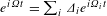
The growth rate of the filamentation instability is expressed by $\unicode[STIX]{x1D6FE}_{F}\cong \unicode[STIX]{x1D6FD}\sqrt{\unicode[STIX]{x1D6FC}/\unicode[STIX]{x1D6FE}_{b}}\unicode[STIX]{x1D714}_{pe}$
, where
$\unicode[STIX]{x1D6FE}_{F}\cong \unicode[STIX]{x1D6FD}\sqrt{\unicode[STIX]{x1D6FC}/\unicode[STIX]{x1D6FE}_{b}}\unicode[STIX]{x1D714}_{pe}$
, where $\unicode[STIX]{x1D6FD}=v_{be}/c$
,
$\unicode[STIX]{x1D6FD}=v_{be}/c$
, $\unicode[STIX]{x1D6FC}=n_{be}/n_{p}$
,
$\unicode[STIX]{x1D6FC}=n_{be}/n_{p}$
, $n_{be}$
is the electron beam number density,
$n_{be}$
is the electron beam number density, $n_{p}$
the number density of the background plasma electrons,
$n_{p}$
the number density of the background plasma electrons, $\unicode[STIX]{x1D6FE}_{b}=1/\sqrt{1-\unicode[STIX]{x1D6FD}^{2}}$
, and
$\unicode[STIX]{x1D6FE}_{b}=1/\sqrt{1-\unicode[STIX]{x1D6FD}^{2}}$
, and $\unicode[STIX]{x1D714}_{pe}$
the plasma frequency of the background plasma electrons.
$\unicode[STIX]{x1D714}_{pe}$
the plasma frequency of the background plasma electrons.
Figure 9 shows the dynamic stabilization mechanism for the filamentation instability schematically. The input electron beam is injected into a plasma, and the electron beam has a current modulation in the $y$
direction. The electron beam current modulation defines actively the filamentation phase as shown in Figure 9(a). After a short time of
$y$
direction. The electron beam current modulation defines actively the filamentation phase as shown in Figure 9(a). After a short time of $\unicode[STIX]{x0394}t$
, the filamentation instability grows. Then the electron beam oscillates in the
$\unicode[STIX]{x0394}t$
, the filamentation instability grows. Then the electron beam oscillates in the $y$
direction as shown in Figure 9(b), and the electron beam modulation also moves in the
$y$
direction as shown in Figure 9(b), and the electron beam modulation also moves in the $y$
direction. The new perturbation with the shifted phase is applied, and the perturbations grow. The overall instability growth should be defined by the sum of all the perturbations at
$y$
direction. The new perturbation with the shifted phase is applied, and the perturbations grow. The overall instability growth should be defined by the sum of all the perturbations at $t$
, and the filamentation instability is dynamically stabilized as shown in Figure 1(c).
$t$
, and the filamentation instability is dynamically stabilized as shown in Figure 1(c).
In order to verify the filamentation instability stabilization, we perform 2-dimensional particle-in-cell (PIC) simulations. As an example case, we use the following parameter values: $\unicode[STIX]{x1D6FC}=n_{be}/n_{p}=1/9$
,
$\unicode[STIX]{x1D6FC}=n_{be}/n_{p}=1/9$
, $\unicode[STIX]{x1D6FD}=v_{be}/c=0.9$
,
$\unicode[STIX]{x1D6FD}=v_{be}/c=0.9$
, $v_{pe}/c=-0.1$
, the temperatures of the beam electrons, the background electrons and the background ions are 100 eV. In our simulations,
$v_{pe}/c=-0.1$
, the temperatures of the beam electrons, the background electrons and the background ions are 100 eV. In our simulations, $n_{p}=1.00\,\times \,10^{-3}\,\times \,4\unicode[STIX]{x1D70B}^{2}\unicode[STIX]{x1D716}_{0}m_{e}c^{2}/(\unicode[STIX]{x1D706}e)^{2}$
, the time is normalized by
$n_{p}=1.00\,\times \,10^{-3}\,\times \,4\unicode[STIX]{x1D70B}^{2}\unicode[STIX]{x1D716}_{0}m_{e}c^{2}/(\unicode[STIX]{x1D706}e)^{2}$
, the time is normalized by $1/\unicode[STIX]{x1D714}_{pe}$
and the scale length is normalized by
$1/\unicode[STIX]{x1D714}_{pe}$
and the scale length is normalized by $\unicode[STIX]{x1D706}$
.
$\unicode[STIX]{x1D706}$
.
Figures 10–12 show the simulation results for the filamentation instabilities with and without the electron beam oscillation. The electron beam perturbation is imposed in the beam density, and the amplitude is 10%. The oscillation amplitude is $5\unicode[STIX]{x1D706}$
in the
$5\unicode[STIX]{x1D706}$
in the $y$
direction in these specific cases. The electron beam oscillation frequency
$y$
direction in these specific cases. The electron beam oscillation frequency $\unicode[STIX]{x1D6FA}$
is
$\unicode[STIX]{x1D6FA}$
is $2\unicode[STIX]{x1D714}_{pe}$
,
$2\unicode[STIX]{x1D714}_{pe}$
, $10\unicode[STIX]{x1D714}_{pe}$
and
$10\unicode[STIX]{x1D714}_{pe}$
and $20\unicode[STIX]{x1D714}_{pe}$
(
$20\unicode[STIX]{x1D714}_{pe}$
( ${>}\unicode[STIX]{x1D6FE}_{F}$
). Figure 10 presents the current density for the cases without and with the electron beam oscillation in the
${>}\unicode[STIX]{x1D6FE}_{F}$
). Figure 10 presents the current density for the cases without and with the electron beam oscillation in the $y$
direction. Figure 11 show the magnetic field
$y$
direction. Figure 11 show the magnetic field $B_{z}$
distribution. The stabilization effect of the filamentation instability is clearly demonstrated in Figure 11. Figure 12 shows the magnetic field energy history. The dynamic stabilization ratio is introduced by
$B_{z}$
distribution. The stabilization effect of the filamentation instability is clearly demonstrated in Figure 11. Figure 12 shows the magnetic field energy history. The dynamic stabilization ratio is introduced by $R_{r}=[1-(U_{Bz}/U_{Bz0})]\times 100\%$
, where
$R_{r}=[1-(U_{Bz}/U_{Bz0})]\times 100\%$
, where $U_{Bz}$
shows the magnetic field energy.
$U_{Bz}$
shows the magnetic field energy. $U_{Bz}$
is normalized by the magnetic field energy
$U_{Bz}$
is normalized by the magnetic field energy $U_{Bz0}$
obtained without the electron beam oscillation. At
$U_{Bz0}$
obtained without the electron beam oscillation. At $t=35\unicode[STIX]{x1D714}_{pe}^{-1}$
, the stabilization ratio
$t=35\unicode[STIX]{x1D714}_{pe}^{-1}$
, the stabilization ratio $R_{r}=58.6\%$
in the case of
$R_{r}=58.6\%$
in the case of $\unicode[STIX]{x1D6FA}=2\unicode[STIX]{x1D714}_{pe}$
. When the electron beam transverse oscillation frequency
$\unicode[STIX]{x1D6FA}=2\unicode[STIX]{x1D714}_{pe}$
. When the electron beam transverse oscillation frequency $\unicode[STIX]{x1D6FA}$
in the
$\unicode[STIX]{x1D6FA}$
in the $y$
direction becomes larger than or comparable to
$y$
direction becomes larger than or comparable to $\unicode[STIX]{x1D6FE}_{F}$
, the dynamic stabilization effect is remarkable. Figure 13 presents the 3D PIC simulation results for the filamentation instability under the same parameter values as those in Figures 10–12. The results shown in Figures 10–13 demonstrate that the dynamic stabilization mechanism works well to stabilize the filamentation instability.
$\unicode[STIX]{x1D6FE}_{F}$
, the dynamic stabilization effect is remarkable. Figure 13 presents the 3D PIC simulation results for the filamentation instability under the same parameter values as those in Figures 10–12. The results shown in Figures 10–13 demonstrate that the dynamic stabilization mechanism works well to stabilize the filamentation instability.
4 Discussions and summary
In this paper we have discussed the dynamic stabilization in plasmas. The dynamic stabilizations[Reference Wolf1–Reference Betti, McCrory and Verdon4], based on the ‘Kapitza’s pendulum’[Reference Kapitza21], introduce a new strong oscillating force into the basic equation, and then the governing equation is modified by the additional term to create a new stable window in the system. Therefore, the growth rate is modified, and the stable window appears in the system. The dynamic stabilization mechanism has been applied to the inverted pendulum[Reference Kapitza21], to a fuel target implosion in laser inertial fusion[Reference Betti, McCrory and Verdon4], and also to the stabilization of the two-stream instability[Reference Qing and Davidson27]. Another dynamic stabilization mechanism, which is also based on the strong forced field but is different from the ‘Kapitza’s pendulum’, was also proposed and applied to a new field in a dissipative dynamic system to find a stable region in the system[Reference Esirkepov and Bulanov30–Reference Krechetnikov and Marsden32]. On the other hand, the dynamic stabilization mechanism based on the phase control was proposed and applied to the stabilization of plasma instabilities including the RTI, the filamentation instability, and also the fuel target implosion in heavy ion inertial fusion (HIF)[Reference Kawata, Karino and Ogoyski20, Reference Kawata22, Reference Kawata, Gu, Li, Karino, Katoh, Limpouch, Klimo, Margarone, Yu, Kong, Weber, Bulanov and Andreev23, Reference Kawata and Karino29]. Originally the dynamic stabilization mechanism comes from the imperfect feedback control, which is widely used to stabilize tall buildings, structures, etc. in our society. In the perfect feedback control, the displacement and its phase are measured, and the additional perturbation is added to stabilize the systems. In plasmas we cannot measure the perturbation phase and amplitude. As we discussed in this paper, we can actively apply the perturbations. Before moving to the system disruption or before developing the nonlinear phase, the additional perturbations, which should have the reverse phase, are applied actively, and then the superimposed total amplitude could be mitigated.
Acknowledgements
This work was partly supported by MEXT, JSPS Kakenhi 15K05359, ILE/Osaka University, CORE/Utsunomiya University, and Japan–U.S. Fusion Research Collaboration Program conducted by MEXT, Japan. This work was partly supported by the project ELITAS (CZ.02.1.01/0.0/0.0/16_013/0001793) and by the project High Field Initiative (CZ.02.1.01/0.0/0.0/15_003/0000449) both from European Regional Development Fund. This project has also partly received funding from the European Union’s Horizon 2020 research and innovation programme under grant agreement No. 633053 (EURO fusion project CfP-AWP17-IFE-CEA-01). Computational resources were provided by the IT4Innovations Centre of Excellence under projects CZ.1.05/1.1.00/02.0070 and LM2011033 and by ECLIPSE cluster of ELI-Beamlines. The EPOCH code was developed as part of the UK EPSRC funded projects EP/G054940/1. The authors would like to appreciate X. F. Li, H. Katoh, J. Limpouch, O. Klimo, D. Margarone, Q. Yu, Q. Kong, S. Weber, S. Bulanov, and A. Andreev for their fruitful discussions on this subject.


 Open access