


1 Introduction
The relativistic electrons generated from the intense short pulse (SP) laser interactions have been extensively studied for a wide range of applications, such as the fast ignition inertial confinement fusion scheme[Reference Tabak, Hammer, Glinsky, Kruer, Wilks, Woodworth, Campbell, Perry and Mason1] and the laser driven electron–positron pair production[Reference Chen, Fiuza, Link, Hazi, Hill, Hoatry, James, Kerr, Meyerhofer, Myatt, Park, Sentoku and Williams2]. The exact mechanisms generating these energetic electrons are still unclear, especially the effects of pre-plasmas on the relativistic electrons. The pre-plasma scale length is known to affect the electron acceleration[Reference Kemp, Sentoku and Tabak3, Reference Pukhov, Sheng and Meyer-ter-Vehn4], the electron beam divergence[Reference Debayle, Honrubia, d’Humieres and Tikhonchuk5] and the laser energy absorption[Reference Ping, Shepherd, Lasinski, Tabak, Chen, Chung, Fournier, Hansen, Kemp, Liedahl, Widmann, Wilks, Rozmus and Sherlock6]. However, there are only a few quantitative experimental data available. In the studies of laser–plasma interactions, the scale length is often estimated from simulated density profiles using radiation-hydrodynamic codes, such as HYDRA[Reference Marinak, Haan, Dittrich, Tipton and Zimmerman7], MULTI2D[Reference Ramis, Meyer-ter-Vehn and Ramírez8] and HYADES[Reference Larsen and Lane9], and further simulations using particle-in-cell codes are carried out to investigate the detailed physics. In spite of continuous development in the radiation-hydrodynamic codes, the codes have to be benchmarked against measurements. Also, it is not practical to simulate a large number of target shots using experimental conditions. Therefore, experimental measurements of the plasma density are still needed.
Optical interferometry is the most widely used technique to measure the plasma electron density in magnetic confinement plasma experiments[Reference Brandi, Giammanco, Harris, Roche, Trask and Wessel10, Reference Akiyama, Yasuhara, Kawahata, Nakayama, Okajima, Urabe, Terashima and Shirai11] and laser plasma experiments[Reference Attwood, Sweeney, Auerbach and Lee12–Reference Sarkisov, Leblanc, Ivanov, Sentoku, Bychenkov, Yates, Wiewior, Jobe and Spielman18]. Also, much effort was put in to devise and improve fringe analysis methods[Reference Takeda, Ina and Kobayashi19–Reference Kemao, Wang and Gao23] and Abel inversion techniques[Reference Kalal and Nugent24–Reference El fagrich and Chehouani27]. However, the optical interferometry is underutilized in high-intensity SP laser interactions with solid targets than it should because (1) setting up the interferometry is very time consuming and (2) the probe beam path prevents other diagnostics from being deployed. This is especially true for experiments at user facilities, such as the Jupiter Laser Facility (JLF), Livermore, USA. In addition, most publications on the fringe analysis and Abel inversion techniques focus on details of specific methods but does not give an overview of the entire data analysis procedures assuming that diagnostic users are already familiar with them. As a result it is very difficult for first time users to successfully field the diagnostic and analyze data unless close guidance, for instance advisers to pupils, is provided. These circumstances motivated this paper to give detailed information on how to successfully employ an optical interferometry and analyze data.
The interferometry setup described here employs the modified Mach–Zehnder (M–Z) interferometer[Reference Hariharan28] and single vertical probe beam path to maximize the use of target chamber space. The data is analyzed by utilizing the Fourier transformation (FT)[Reference Takeda, Ina and Kobayashi19] and the linear operator methods[Reference Dasch25]. Readers are strongly encouraged to read the references given in this paper and references therein for more detailed information.
2 Experimental conditions and setup
The experimental scheme and interferometer setup described here have been used in multiple campaigns to investigate the effects of pre-plasmas on energetic electrons generated in laser–solid interactions on the Titan laser[Reference Stuart, Bonlie, Britten, Caird, Cross, Ebbers, Eckart, Erlandson, Molander, Ng, Patel and Price29] at JLF at Lawrence Livermore National Laboratory.
Targets made of aluminum (Al), titanium (Ti), copper (Cu), gold (Au) and plastics (CH) were shaped in disk or square form. The disk targets were made of single material, and their dimension varied between 2 and 6 mm in diameter and  $75~\unicode[STIX]{x03BC}\text{m}$ to 1 mm in thickness. Two different types of square targets ( $3~\text{mm}\times 3~\text{mm}$) with varying thickness between $75~\unicode[STIX]{x03BC}\text{m}$ and 1.28 mm were used for the study: bulk (CH, Ti, or Cu) and layered. The layered targets had $10~\unicode[STIX]{x03BC}\text{m}$ metal foil (Ti or Cu) sandwiched between two plastic layers with a thinner layer (3– $15~\unicode[STIX]{x03BC}\text{m}$) on the laser incident side.
2.1 Short pulse laser conditions
The Titan SP laser uses optical parametric chirped pulse amplification[Reference Dubietis, Jonus̆auskas and Piskarskas30] to generate 0.7–20 ps long pulses and delivers up to 350 J energy on targets when operated at the fundamental wavelength,  $1.054~\unicode[STIX]{x03BC}\text{m}$ ( $1\unicode[STIX]{x1D714}$)[Reference Stuart, Bonlie, Britten, Caird, Cross, Ebbers, Eckart, Erlandson, Molander, Ng, Patel and Price29]. The SP laser beam is focused to a focal spot of 10– $15~\unicode[STIX]{x03BC}\text{m}$ at the full-width-half-maximum (FWHM) by an $\text{F}/3$ off-axis parabola, and the maximum laser intensity of low $10^{20}~\text{W}/\text{cm}^{2}$ is achievable. The SP laser can be operated at the second harmonic, $0.527~\unicode[STIX]{x03BC}\text{m}$.
The pre-plasma experiments were performed using the  $1\unicode[STIX]{x1D714}$ Titan SP laser at its minimum pulse length, and the laser energy on targets was varied between 110 and 140 J. The $1\unicode[STIX]{x1D714}$ SP laser has a nanosecond scale pre-pulse that generated pre-plasmas on the target front surface. The pre-pulse energy history was monitored on each shot with a 20 ps temporal resolution by using a calibrated fast diode (EOT ET-3500) and a fast oscilloscope. The fast diode system was calibrated against a calorimeter placed inside the target chamber under vacuum. The main SP laser was partially amplified, 100–200 mJ, and uncompressed, ${\sim}3$ ns long. The fast diode read-out (V) was integrated and normalized to the measured energy in order to find a scaling factor, J/V. The measured pre-pulse had a nominal pulse length of $3.3\pm 0.5$ ns with energies between 10 and 70 mJ, which was equivalent to laser intensity in a range of $10^{12}{-}10^{13}~\text{W}/\text{cm}^{2}$.
Figure 1 shows a recorded pre-pulse (solid blue curve) and a linear fit (dotted red line) to it. The sharp rise at 0 ns (vertical dashed black line) is due to the arrival of the main pulse. The pre-pulse was  ${\sim}3.2$ ns long and contained $62\pm 6$ mJ.

Figure 1. The pre-pulse measured by the calibrated fast diode (solid blue) and a linear fit (dotted red).
2.2 Sub-picosecond optical probe laser
The interferograms were taken using a laser optical probe. The optical probe is split from a main SP front end (after the beam stretcher) and bypasses the amplification system, which allows the probe laser to arrive prior to the main SP laser. Upon entering the target area, the probe laser propagates through an open air compressor which adjusts the probe laser pulse length for various optical diagnostics. For the interferometry the probe beam was compressed to the minimum pulse length of  ${\sim}0.5$ ps in order to take snapshots of the pre-plasmas. The probe laser was frequency doubled ( $0.527~\unicode[STIX]{x03BC}\text{m}$ or $2\unicode[STIX]{x1D714}$) by a beta barium borate (BBO) crystal in order to increase the maximum measurable plasma density. The relationship between the index of refraction of plasmas, $\unicode[STIX]{x1D702}_{p}$, and the plasma density, $n_{e}$, is given as,
 $$\begin{eqnarray}\unicode[STIX]{x1D702}_{\text{plasma}}=\sqrt{1-\frac{n_{e}}{n_{c}}},\end{eqnarray}$$
 where  $n_{c}$ is the plasma critical density. The critical density is inversely proportional to the square of a probe beam wavelength, $n_{c}\approx 1.12\times 10^{21}/\unicode[STIX]{x1D706}_{\text{probe}}^{2}~\text{cm}^{-3}$, where $\unicode[STIX]{x1D706}_{\text{probe}}$ is the probe laser wavelength in $\unicode[STIX]{x03BC}\text{m}$. The critical density for the frequency doubled probe laser is ${\sim}4\times 10^{21}~\text{cm}^{-3}$.
2.3 Probe beam path
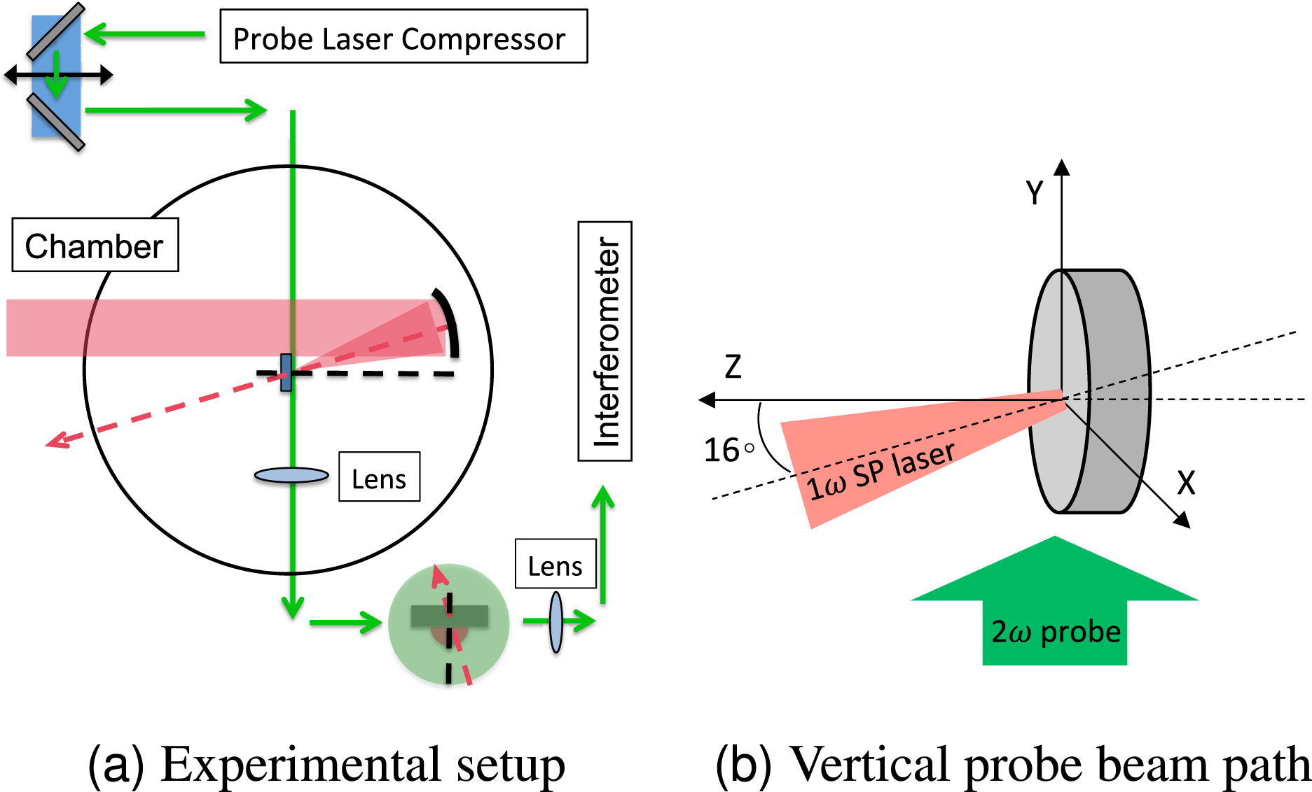
Figure 2. (a) A simplified experimental scheme and (b) the single vertical probe beam path at the target position.
Figure 2(a) shows a simplified top–down view of the experimental setup. The SP laser (red shade) is focused by the F/3 parabola on to a target at  ${\sim}16^{\circ }$ (red dashed arrow) from the target normal (black dashed line). The 0.5 ps $2\unicode[STIX]{x1D714}$ probe laser (green arrows) emerging from the compressor propagates through a timing periscope, which is to adjust the relative timing between the SP and probe lasers at the target area, and enters the target chamber. Inside the chamber the probe beam is initially positioned below the SP laser plane in order to scan pre-plasmas vertically, i.e., perpendicular to the SP beam plane. Figure 2(b) shows the relative orientation of a target, the main SP and probe lasers: the SP laser (red shade) is incident on target at an angle of $16^{\circ }$ from the target normal, and the probe laser travels perpendicular to the SP laser plane ( $x{-}z$ plane). Note that the relative location of the target within the probe beam is important for any single probe path: the target has to be placed on one side of the probe beam in order to make sure a large area of the beam is not perturbed by plasmas. The unperturbed part of the probe beam is used as reference to generate fringes by an interferometer.
The probe beam, after interacting with pre-plasma, is collected by a lens to form the first image with a small magnification,  $\times 2$ to $\times 3$, outside of the chamber. The final image is formed by another lens to give $\times 16$ to $\times 20$ magnification with better than $10~\unicode[STIX]{x03BC}\text{m}$ imaging resolution. An interferometer was placed between the second lens and the imaging plane.
The vertical probe path requires extra effort as comparison to the common coplanar probe beam path. However, it allows to deploy more diagnostics and maximize the experimental time: an x-ray pinhole camera, Figure 2(b), and an x-ray spectrometer (not shown) were used on the SP laser plane close to the target position.
2.4 Laser relative timing
The relative timing between the SP and probe lasers was adjusted by controlling the timing periscope, Figure 2(a), while monitoring the unamplified SP and the probe lasers using a Hamamatsu visible streak camera, C7700-11[31]. Because two laser paths were orthogonal to each other, a light scattering target was used in order to scatter the SP laser light and propagate the scattered light along the probe beam path. The light signals from both lasers were collected by the first lens within the chamber, and the streak camera was placed at the first imaging plane.

Figure 3. An image captured by the streak camera (left top) and laser signals along the vertical line on the image (right bottom) are shown.
Figure 3 shows an image recorded by the streak camera (top left) and line-out along the temporal axis (bottom right). The image was recorded by a charge-coupled device (CCD) with  $1024\times 1024$ pixels and a 500 ps sweeping window. The curvature of streaked lines is due to the edge effect of high voltage applied to the sweep plates within the streak camera. The upper (earlier) streak is the probe beam which was partially blocked by the scattering target (indicated with an arrow).
The plot shows signals from the probe beam (left) and the SP laser (right). The probe beam had a large tail, possibly, due to (1) a part of the probe beam doubly reflected within the BBO crystal, (2) the unconverted  $1\unicode[STIX]{x1D714}$ probe beam whose pulse length was slightly larger than the green light, (3) an artifact of the streak camera, etc. A Gaussian fit with three terms, two for the probe and one for the SP, were used to find the peak locations. The light signals are separated by ${\sim}47$ pixels, equivalent to ${\sim}23$ ps.
2.5 Modified Mach–Zehnder interferometer
The Nomarski interferometer[Reference Benattar, Popovics and Sigel32] and the modified M–Z interferometer[Reference Hariharan28] have been used in earlier experiments. However, the modified M–Z interferometer was chosen for later experiments for the following reasons.
The Nomarski interferometer uses a Wollaston prism to split the probe laser into two orthogonally polarized beams and a pair of polarizers, before and after the prism, to control the probe laser polarization in order to generate fringes. The Nomarski interferometer is easy to work, especially with a sub-picosecond probe laser, because the orthogonally polarized beams have equal path lengths and generate fringes where they overlap. However, control of the image separation (from the separated beams) and the fringe gap are interlinked via the angle at which the prism splits the probe laser; both the image separation and fringe gap become smaller or larger as the prism is brought closer to or further away from the final imaging plane, respectively (Figure 1 in Ref. [Reference Benattar, Popovics and Sigel32]). Therefore, achieving adequate image separation and fringe density could be difficult in cases of relatively large ( ${\sim}1$ mm) targets or plasmas with high magnification ( $\times 15$ or larger) due to image blurring caused by overlapped images.
The M–Z interferometer uses a pair of beam splitters to separate a probe laser into two arms (probing and reference arms) and merge them back to generate fringes, which requires extra attention in order to generate fringes. On the other hand, the M–Z interferometer offers much better control over the image separation and fringe gap than the Nomarski interferometer does. Note that the conventional M–Z interferometer setup of using a pair of mirrors and beam splitters also suffers from the interlinked control of the image separation and fringe spacing. This restriction can be easily removed if a pair of mirrors are replaced with two pentaprisms or two periscopes while keeping the versatility of the M–Z interferometer[Reference Hariharan28]. The details of the diagnostic setup and fringe adjustment are given below.

Figure 4. A modified M–Z interferometer setup.
Figure 4 shows the modified M–Z interferometer with a pair of beam splitters and periscopes as well as images before and after entering the diagnostic. The separation of target images and the fringe spacing at the final imaging plane are controlled rotating both beam splitters (BS1 and BS2) by unequal amounts for the following reasons. Rotating only one beam splitter can lead to unrecognizably small fringes before reaching an appropriate image separation. On the other hand, rotating the beam splitters by equal amounts easily separates the images but does not change the fringe spacing. Therefore, two beam splitters have to be rotated by unequal amounts in order to separate the images and control the fringe spacing. Keep in mind, however, that unequal amounts of rotations will result in low contrast fringes or loss of fringes when an SP probe laser is used because the split probe beams no longer temporally overlap at the final imaging plane. The co-arrival of the split beams (and fringe generation) is achieved by mounting one periscope on a translation stage (Periscope 1 in Figure 4) and simultaneously adjusting its position while rotating the beam splitters.
3 Fringe analysis
The index of refraction through plasmas differ from that of vacuum or air. The difference in the index of refraction causes the probe beam to experience different optical path length and shifts fringes. Therefore, the fringe analysis is done in two stages: estimation of (1) the probe beam path length change and (2) the index of refraction. Once the refractivity is found, the plasma density is estimated using the relationship given in Equation (1).
Note that fringe data analysis procedures are to find the index of refraction, and a physical variable of interest depends on how the index of refraction is expressed. For instance, one can estimate the plasma density (as in this paper) while others estimate temperatures if the index of refraction is expressed in terms of temperature[Reference Posner and Dunn-Rankin33].
3.1 Phase map: Fourier transformation method
The path length difference can be estimated by counting the number of fringe shift,  $N=\unicode[STIX]{x1D6E5}P$. However, counting fringes could be erroneous and time consuming. Takeda et al. [Reference Takeda, Ina and Kobayashi19] suggested a more elegant way of estimating the phase difference, $\unicode[STIX]{x1D6E5}\unicode[STIX]{x1D711}=(2\unicode[STIX]{x1D70B}/\unicode[STIX]{x1D706}_{\text{probe}})\unicode[STIX]{x1D6E5}\text{P}$, at each point on interferograms by using the FT method. The FT method is not only faster than the direct fringe shift counting method but also reduces noises from interferograms. In addition, the phase difference estimated by using the FT method forms a smooth curve at the target boundary and beyond, as seen in Figures 5(b) and 5(c), while the direct counting method would result in an abrupt change in the estimated phase difference. As result, the FT method helps eliminating spiky features when the Abel inversion is used to extracted profiles (the plasma density profile in this paper). Note that a proper mask should be employed in order to separate the erroneous regions out of the unfolded density profile as the phase difference beyond boundaries are not correct values.

Figure 5. Interferogram and phase maps. The red dotted line in (a) indicates the original target–vacuum interface.
The FT method uses the oscillatory nature of fringes to estimate the phase value in four steps: (1) forward FT of an interferogram,  $\text{FT}_{\text{inter}}$, (2) selection of one side in the frequency domain, (3) inverse FT of one-sided frequency spectrum, $\text{FT}_{\text{inter}}^{-1}$ and (4) the phase value extraction. When interferograms are Fourier transformed, there are three distinctive peaks: at the zero frequency and at the nascent frequencies, $\pm f_{o}$. Selecting one side of spectrum with an adequate width, $f_{o}\pm \unicode[STIX]{x1D6E5}f$, and performing the inverse FT reduces noise with components faster or slower than the fringe frequency but retains the fringes. The phase at each point is found by taking the imaginary part after applying the natural logarithm to the inverse FT of one-sided frequency spectrum, $f_{o}+f_{1}=\text{Im}[\ln (\text{FT}_{\text{inter}}^{-1})]$, where $f_{1}$ is due to the fringe shift. The real part, $\text{Re}[\text{FT}_{\text{inter}}^{-1}]$, reconstructs interferograms with reduced noise, which can be used to check the adequacy of the frequency width, $\pm \unicode[STIX]{x1D6E5}f$[Reference Kalal and Nugent24]. Consult[Reference Takeda, Ina and Kobayashi19] and appendix in Ref. [Reference Antici, Chen, Gremillet, Grismayer, Mora, Audebert and Fuchs34] for more detailed information.
Figure 5 shows an interferogram recorded by a CCD with  $7.4~\unicode[STIX]{x03BC}\text{m}$ per pixel and an estimated phase map by using the FT method. The red dotted line in Figure 5(a) indicates the original target surface, and the bright spot is caused by the plasma emission near the probe beam wavelength, $0.527~\unicode[STIX]{x03BC}\text{m}$. A few different methods were employed in order to reduce the recorded plasma emission. First, $2\unicode[STIX]{x1D714}$ specific optics, such as mirrors, lens, beam splitters and $527\pm 5$ nm filters, were used along the probe path after the target area. Second, a waveplate and a polarizer were used before and after the target area, respectively, in order to remove $2\unicode[STIX]{x1D714}$ plasma emission at different polarization. Also, an aperture was used at the light converging point of the first lens.
Notice that the phase values oscillate between 0 and  $2\unicode[STIX]{x1D70B}$ (or $-\unicode[STIX]{x1D70B}$ and $\unicode[STIX]{x1D70B}$), Figure 5(b). Therefore, it is necessary to remove the discontinuities between 0 and $2\unicode[STIX]{x1D70B}$ by adding or subtracting $2\unicode[STIX]{x1D70B}$, ‘phase unwrapping’[Reference Judge and Bryanston-Cross35], in order to find the phase difference, $\unicode[STIX]{x1D6E5}\unicode[STIX]{x1D711}$. Figure 5(c) shows the final unwrapped phase map of the interferogram.
Once unwrapped phase maps are obtained from the reference and shot interferograms, the phase difference is estimated by subtracting the two,  $\Vert \unicode[STIX]{x1D6E5}\unicode[STIX]{x1D711}\Vert =\Vert \unicode[STIX]{x1D711}_{\text{reference}}-\unicode[STIX]{x1D711}_{\text{shot}}\Vert$. Note that the phase difference could be either positive or negative depending on how fringes shift, convex or concave, and the order of the phase subtraction. Therefore, the absolute value of the phase difference is used here in order to remove any ambiguity due to the sign convention.
Notice that the word ‘phase’ was used for two different things: the phase of fringes and the probe beam path length (difference). Readers should be mindful how ‘phase’ is used in the context and which definition it refers to.
3.2 Plasma index of refraction: linear operator method

Figure 6. A cylindrical geometry and the Abel transformation variables.
The phase of the probe laser propagating through plasmas with a cylindrical symmetry, Figure 6, can be expressed by the Abel transform, and the plasma index of refraction,  $\unicode[STIX]{x1D702}$, can be estimated by performing the inverse Abel transform. The Abel forward and inverse transform equations are expressed as, respectively,
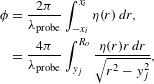 $$\begin{eqnarray}\displaystyle \unicode[STIX]{x1D711} & = & \displaystyle \frac{2\unicode[STIX]{x1D70B}}{\unicode[STIX]{x1D706}_{\text{probe}}}\int _{-x_{i}}^{x_{i}}\unicode[STIX]{x1D702}(r)\,dr,\nonumber\\ \displaystyle & = & \displaystyle \frac{4\unicode[STIX]{x1D70B}}{\unicode[STIX]{x1D706}_{\text{probe}}}\int _{y_{j}}^{R_{o}}\frac{\unicode[STIX]{x1D702}(r)r\,dr}{\sqrt{r^{2}-y_{j}^{2}}},\end{eqnarray}$$
 $$\begin{eqnarray}\displaystyle \unicode[STIX]{x1D702} & = & \displaystyle 2\unicode[STIX]{x1D706}_{\text{probe}}\int _{r}^{R_{0}}\frac{\unicode[STIX]{x1D6FF}\unicode[STIX]{x1D711}/\unicode[STIX]{x1D6FF}y}{\sqrt{y^{2}-r^{2}}}\,dy,\end{eqnarray}$$
 where a target surface is on the  $X{-}Z$ plane. The Abel inversion has two short comings: it requires the derivatives of the phase, $\unicode[STIX]{x1D6FF}\unicode[STIX]{x1D711}/\unicode[STIX]{x1D6FF}y$, and the integrand diverges along the symmetric axis, $y\rightarrow r$. These problems can be overcome if a linear operator method is used.
Dasch[Reference Dasch25] showed that the inverse Abel transform could be represented as a linear operator if any line-of-sight projected data is taken at equal spacing,
 $$\begin{eqnarray}\unicode[STIX]{x1D702}_{\text{plasma}}(r_{i})=\frac{1}{\unicode[STIX]{x1D6E5}r}\mathop{\sum }_{j=0}^{\infty }\mathbf{D}_{ij}\unicode[STIX]{x1D711}(r_{ij}),\end{eqnarray}$$
 where  $\unicode[STIX]{x1D6E5}r$ is the data spacing (CCD pixel size/magnification), $r_{i}=i\unicode[STIX]{x1D6E5}r$ is the distance from the symmetric axis, and $\mathbf{D}_{ij}$ are the linear operator coefficients. The coefficients depend on the numerical algorithm used to calculate but are independent of the data spacing. Therefore, they can be pre-calculated and stored for future use.
The change in the index of refraction due to plasmas,  $\Vert \unicode[STIX]{x1D6E5}\unicode[STIX]{x1D702}\Vert$, is estimated by applying the linear operator to the phase difference, $\Vert \unicode[STIX]{x1D6E5}\unicode[STIX]{x1D711}\Vert$, and the plasma index of refraction is calculated by using a relationship, $\unicode[STIX]{x1D702}_{\text{plasma}}=1-\unicode[STIX]{x1D6E5}\unicode[STIX]{x1D702}$. Finally, the plasma density is calculated by using Equation (1).
Figure 7 shows the plasma density profile estimated from the interferogram shown in Figure 5. The Onion Peeling linear operator was chosen among several operators presented by Dasch. The right end of the profile,  $x=0~\unicode[STIX]{x03BC}\text{m}$, is at the target–vacuum interface, and the origin, $(0,0)~\unicode[STIX]{x03BC}\text{m}$, is centered at the laser focal spot. The red dotted curve indicates the last visible fringe used as a masking line, ${\sim}3\times 10^{19}~\text{cm}^{-3}$, beyond which the plasma density becomes erroneous due to the refraction of the probe beam and plasma emission. The plasma density up to $5\times 10^{19}~\text{cm}^{-3}$ was measured during experiments, which is similar to other studies using optical interferometry[Reference Le Pape, Tsui, Macphee, Hey, Patel, Mackinnon, Key, Wei, Ma, Beg, Stephens, Akli, Link, Van-Woerkom and Freem36, Reference Fuchs, d‘Humières, Sentoku, Antici, Atzeni, Bandulet, Depierreux, Labaune and Schiavi37]. The measurement near the density of $1\times 10^{21}~\text{cm}^{-3}$ requires shorter wavelength probe beam, such as soft x-ray[Reference Da Silva, Barbee, Cauble, Celliers, Ciarlos, Libby, London, Matthews, Mrowka, Moreno, Ress, Trebes, Wan and Webber38].
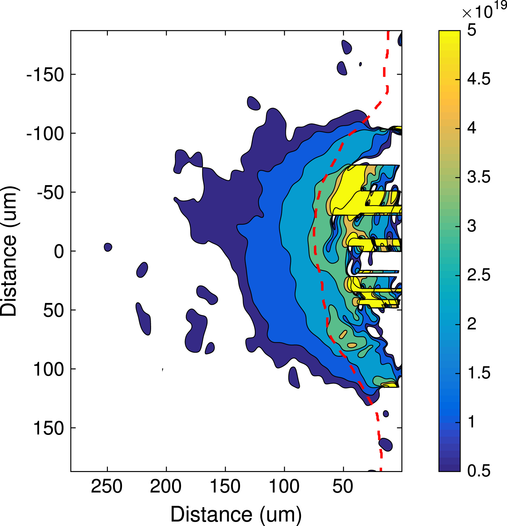
Figure 7. Two dimensional plasma density  $(\text{cm}^{-3})$ profile extracted from the interferogram shown in Figure 5. The white color indicates densities below $5\times 10^{18}~\text{cm}^{-3}$.
4 Summary
An optical interferometry with the vertical single probe path and the modified M–Z interferometer has been successfully used in multiple campaigns. This scheme allowed more diagnostics to be simultaneously fielded than the horizontal probe path would have. The plasma density measurements provided valuable data to benchmark radiation-hydrodynamic simulation. The experimental measurements and simulation of the plasma density together played crucial roles to investigate the effects of pre-plasmas on the relativistic electrons, which is a subject of future publication.
Acknowledgments
The authors give special thanks to the JLF staff for the support and Ronnie Shepherd, James Dunn, Klaus Widmann, Sebastian Le Pape and Yuan Ping for discussions. The authors appreciate the reviewers for valuable comments to improve this manuscript. J. Park is also grateful for the support from the LDRD (15-ERD-054) program to finish the manuscript. This work was performed under the auspices of the US DOE by LLNL under contract no. DE-AC52-07NA27344 and funded by the LDRD (12-ERD-062) program.


 Open access