


1 Introduction
Coherent beam combining (CBC) is one of the most promising techniques for laser power scaling, which can break through the physical limitations of a single beam while maintaining excellent laser characteristics[ Reference Klenke, Müller, Stark, Kienel, Jauregui, Tünnermann and Limpert 1 – Reference Fathi, Närhi and Gumenyuk 3 ]. Due to internal and external perturbations, such as spontaneous emission[ Reference Li, Fu, Zhu, Fang, Zhu, Zhong, Xu, Chen, Wang and Zhan 4 ], quantum defect[ Reference Tünnermann, Neumann, Kracht and Weßels 5 ], environment temperature fluctuation[ Reference Llopis, Merrer, Brahimi, Saleh and Lacroix 6 ] and mechanical and acoustical vibrations[ Reference Lombard, Canat, Durecu and Bourdon 7 ], laser phases change dynamically in practical operation[ Reference Zhou, Tao, Zhang, Xie, Feng, Wen, Chu, Lin, Wang, Yan and Jing 8 ], which severely impairs the combining efficiency and makes the CBC laser system unstable, or even disabled[ Reference Augst, Fan and Sanchez 9 ]. Active phase control is an efficient solution to phase synchronization and stabilization of multiple lasers in real time, and various control methods have been developed and demonstrated[ Reference Antier, Bourderionnet, Larat, Lallier, Lenormand, Primot and Brignon 10 – Reference Ma, Chang, Ma, Su, Qi, Wu, Li, Long, Lai, Chang, Hou, Zhou and Zhou 15 ]. Facilitated by the rapid development of active phase-control techniques, several milestones of CBC have been achieved. The maximal average power of 10 kW has been achieved in ultrashort pulse regimes, while active control of up to 1000 channels has been demonstrated[ Reference Müller, Aleshire, Klenke, Haddad, Légaré, Tünnermann and Limpert 16 , Reference Chang, Gao, Deng, Ren, Ma, Su, Ma and Zhou 17 ]. For some advanced applications, such as laser particle accelerators and coherent amplification networks, higher power and more channels are required[ Reference Mourou, Brocklesby, Tajima and Limpert 18 – Reference Mourou 23 ]. Generally, faster active phase control is demanded as the channel number scales, and traditional control methods encounter great challenges in terms of phase-control bandwidth or complexity[ Reference Zhou, Liu, Wang, Ma, Ma, Xu and Guo 24 – Reference Zhou, Feng, Xie, Li, Zhang, Tao, Lin, Wang, Yan and Jing 26 ].
To further increase the phase-control bandwidth while maintaining simple configuration, machine learning, including reinforcement learning and deep learning, has been applied in the field of CBC phase control[ Reference Tunnermann and Shirakawa 27 – Reference Jiang, Gao, Tan, Zhang, Dou, Di and Qin 32 ]. Machine learning is a versatile technique that automatically learns and extracts complicated features from data, enabling the agent/network to make phase predictions based on system state information such as diffractive patterns or other intensity observations[ Reference Tünnermann and Shirakawa 33 , Reference Wang, Du, Zhou, Li and Wilcox 34 ]. Direct phase recovery is achievable once the mapping from system state to phase action is established through learning, offering significant advantages of simple optics structure and minimal convergence steps without time-consuming iterations[ Reference Shpakovych, Maulion, Kermene, Boju, Armand, Desfarges-Berthelemot and Barthélemy 35 ]. Theoretically, only one step is required to optimize the phase, which is independent of the number of the channels, making it the most promising control technology for large-scale CBC applications[ Reference Xie, Chernikov, Mills, Liu, Praeger, Grant-Jacob and Zervas 31 , Reference Mills, Grant-Jacob, Praeger, Eason, Nilsson and Zervas 36 ]. Deep learning is initially integrated into CBC systems by utilizing non-focal-plane data for training, and 7- and 19-channel CBC phase control is numerically demonstrated with Strehl ratios of 0.98 and 0.84, respectively[ Reference Hou, An, Chang, Ma, Li, Zhi, Huang, Su, Wu, Ma and Zhou 37 ]. One-hundred-channel CBC has been experimentally achieved with a residual phase of λ/30, which represents the maximal number of beams controlled by machine learning[ Reference Shpakovych, Maulion, Kermene, Boju, Armand, Desfarges-Berthelemot and Barthélemy 35 ]. To date, the majority of applications have focused on tiled-aperture CBC systems[ Reference Zuo, Jia, Geng, Bao, Zou, Li, Jiang, Li, Li and Li 29 – Reference Jiang, Gao, Tan, Zhang, Dou, Di and Qin 32 , Reference Shpakovych, Maulion, Kermene, Boju, Armand, Desfarges-Berthelemot and Barthélemy 35 – Reference Hou, An, Chang, Ma, Li, Zhi, Huang, Su, Wu, Ma and Zhou 37 ]. In contrast, filled-aperture CBC offers the highest combining efficiency as it eliminates energy loss due to sidelobes[ Reference Redmond, Ripin, Yu, Augst, Fan, Thielen, Rothenberg and Goodno 38 – Reference Liu, Ma, Su, Tao, Ma, Wang and Zhou 40 ], which is particularly crucial for power scaling applications. However, in filled-aperture CBC, all sub-beams overlap completely in both the near field and far field, resulting in a combined beam pattern that contains minimal phase information, which has limited the utilization of machine learning in filled-aperture CBC. It is noteworthy that machine learning methods typically yield a larger residual phase compared to traditional approaches, prompting researchers to devise a two-stage control scheme to improve accuracy, albeit with increased complexity[ Reference Hou, An, Chang, Ma, Li, Huang, Zhi, Wu, Su, Ma and Zhou 28 ].
In this paper, a deep learning algorithm is modified to suppress the residual phase and is applied in a filled-aperture CBC system with an innovative design in optics structure and control scheme that can achieve phase-locking in a single step with high accuracy. The trained network can predict phase with an error of λ/70 in a single step for a nine-channel filled-aperture CBC, illustrating the effectiveness of the proposed method. To the best of our knowledge, this represents the first demonstration of machine learning phase control in a filled-aperture CBC scenario with high accuracy.
2 Principle
2.1 System setup
The system structure of filled-aperture CBC based on deep learning phase control is depicted in Figure 1. The seed laser is split into multiple beam channels by a beam splitter (BS), and each beam path passes through a phase modulator (PM), amplifier and collimator (CO). All beams are tiled in a dense array, such as square shape[ Reference Bourderionnet, Bellanger, Primot and Brignon 25 ], hexagon shape[ Reference Ma, Chang, Ma, Su, Qi, Wu, Li, Long, Lai, Chang, Hou, Zhou and Zhou 15 ] or others[ Reference Li, Liao, Gao, Sun, Tan, Wang and Lan 41 ], and are then emitted in the same direction. The laser array is sampled before coming into the filled-aperture beam combiner to obtain the tiled-aperture combined pattern by a camera, which is input into the neural network to make phase prediction and compensate phase noise with high-bandwidth operation. The combiner can take a variety of forms, such as diffractive optical element (DOE)[ Reference Thielen, Ho, Burchman, Goodno, Rothenberg, Wickham, Flores, Lu, Pulford, Robin, Sanchez, Hult and Rowland 42 ], intensity BS-based binary tree or segmented mirror[ Reference Müller, Aleshire, Klenke, Haddad, Légaré, Tünnermann and Limpert 16 ], which transforms spatially separated beams into an overlapped beam. The segmented mirror combiner is employed in this paper since it is easy to combine a laser array of linear or square tiling, which will be superimposed into a single beam at one output port if amplitudes match the splitting ratios and phases are locked; it is only represented by a box in Figure 1 for simplicity, and its specific architecture can be found in Ref. [Reference Aleshire, Steinkopff, Jauregui, Klenke, Tünnermann and Limpert43]. A liquid crystal (LC) is inserted in the sampled path of each spatially separated beam, so the optical path delays of all beams can be artificially adjusted. The laser array of main power illuminates on the beam combiner and is combined into a single aperture beam in the near field, and the central intensity of the combined beam is sampled by a photodetector (PD), which is used to drive the delay controller and monitor the combining efficiency.
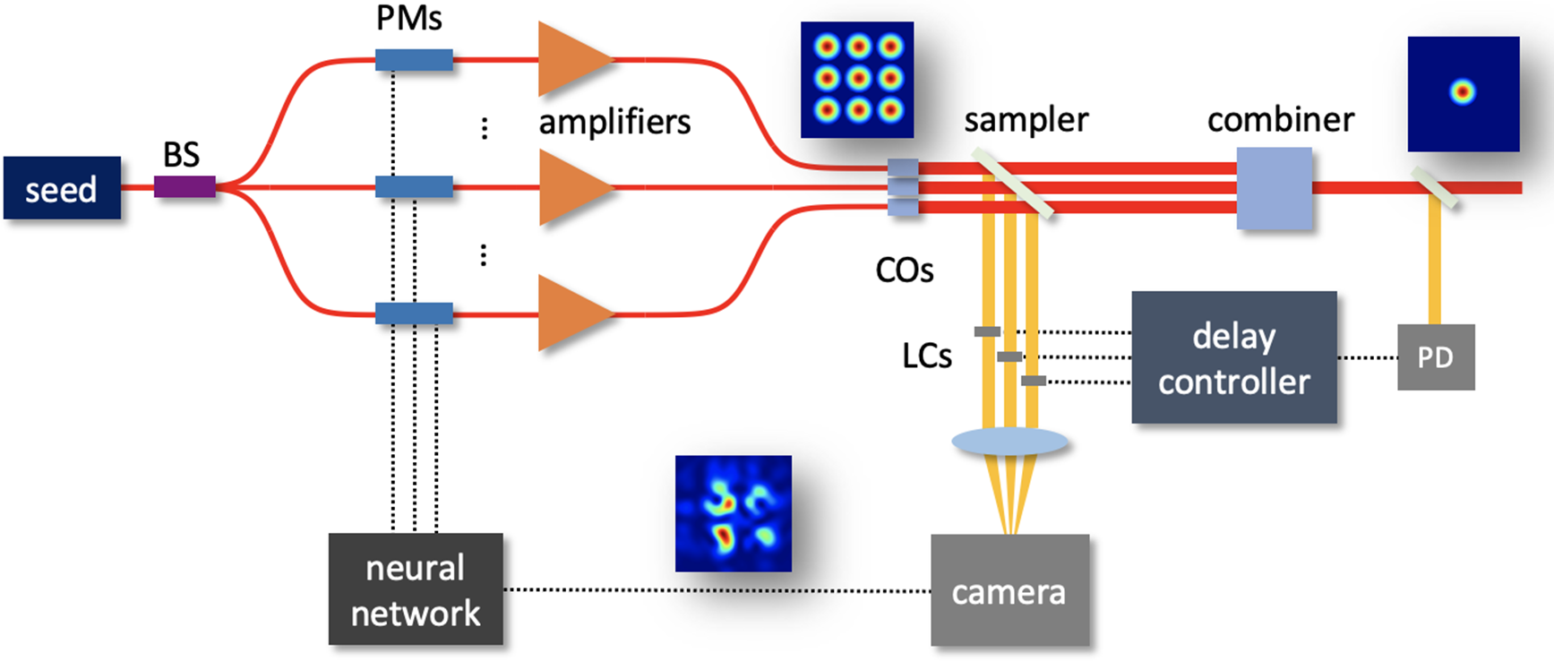
Figure 1 System setup of deep learning phase control for filled-aperture CBC.
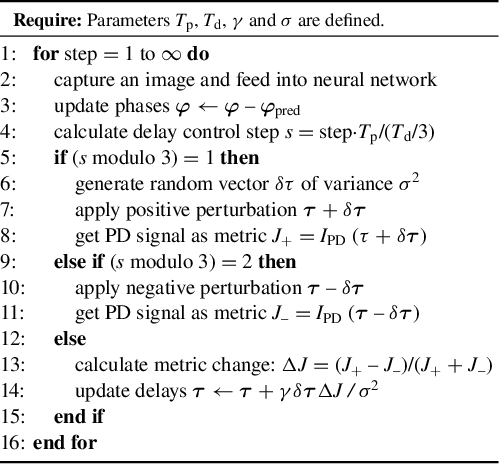
As the beam combiner needs to fill the aperture, each beam passes through its own combining route, which results in different optical paths and laser phases. Therefore, the phase relationships at the camera are not consistent with those at the PD due to optical path differences, which accounts for why the delay control is essential to compensate for the static path-related phases. It should be noted that although the optical path difference dominantly occurs inside the combiner, it can be eliminated by adjusting the phase delays in the sampled path instead, which is consistent with high-power operation due to the avoidance of manipulation on high-power beams. The delay control is an optimization problem of multiple variables, and thus stochastic parallel gradient descent (SPGD) can be employed to address the issue conveniently. The process of delay control is described in the flow chart in Table 1, where T p/T d denotes the time step of phase/delay update, and γ and σ are the gain coefficient and perturbation amplitude, respectively, of the SPGD algorithm. As the SPGD algorithm requires two-way perturbations before parameter update, one step of delay control is divided into three mini-steps, so the current step of delay control is calculated according to T d/3, as shown in line 4 of Table 1. The phase control is much faster than delay control (T p ≪ T d), so phase-locking is achieved immediately after the delays are perturbed or updated. It should be emphasized that the PD signal does not change directly with delays of LCs but changes with phases of PMs, since the neural network will dynamically drive PMs to compensate for the delay changes and maintain phase-locking at the camera.
Table 1 Procedure for delay control.
With the delay control done, the phase relationships at the tiled-aperture path (camera) are the same as at the filled-aperture path (PD), and thus the filled-aperture combining efficiency will be maximized when laser phases are synchronized at the camera by the neural network. Therefore, filled-aperture phase control can be converted into tiled-aperture phase control with proper delay control. In addition, optical path length differences in the combiner are generally piston errors, so the delay control can be implemented in a once and forever manner theoretically, and only phase control is required finally.
2.2 Training strategies
Although the mapping from the combined pattern to laser phases can be interpreted as a pattern recognition problem, there are two barriers to cross when applying deep learning to the phase control of CBC. The first is the phase periodicity-induced discontinuity, where φ and φ + 2kπ (k = 0, ±1, ±2, ⋯) represent the same phase, but their distance is 2kπ. In general, phase is limited to a single period [–π, π) so that every value will correspond to a unique phase, but this does not work well in the training of neural networks as the distance between label and output is usually used to calculate loss. For instance, if the network predicts 0.9π as –π, the prediction is actually good because it is equivalent to –1.1π and –π with a real distance of 0.1π, but it will result in a large loss because the network interprets the distance as 1.9π. To deal with this, a sin-cos loss is introduced and defined as follows:
 $$\begin{align}L=\frac{1}{2M\left(N-1\right)}\sum \limits_{m=1}^M\sum \limits_{n=1}^{N-1}&\left[{\left|\sin {\varphi}_n^{(m)}-\sin {\varphi}_n^{\ast (m)}\right|}^2\right.\nonumber\\& \ \ \left.+{\left|\cos {\varphi}_n^{(m)}-\cos {\varphi}_n^{\ast (m)}\right|}^2\right]\end{align}$$
where φ* and φ are the true phase and the predicted phase, respectively, subscript n denotes the beam number (the total is N–1 as one beam is set as reference) and superscript m denotes the sample number (the total is batch size M).
The proposed loss function calculates both sine and cosine distances between the network output and true phase, which is inducive to overcome the aforementioned phase discontinuity, since phase is not compared directly. However, if the network is requested to output phase predictions φ, the discontinuity remains unsolved. More specifically, phases of around –π and π should be predicted using similar image features with the same network parameters, so the network will struggle to minimize losses at both ends rather than learning an accurate and unique mapping function, which means that the learning problem is not a strict one-to-one mapping, so the learning process is not very good. Therefore, the output of the network is designed to consist of both the sine and cosine of phase φ. It should be noted that the sine and cosine values may not strictly satisfy the equation of sin2 φ + cos2 φ = 1, as they are predicted independently by the neural network. Letting C and S represent the predicted cosine of phase (cosφ) and predicated sine of phase (sinφ), respectively, although C and S probably correspond to different predicated phases, a more accurate phase prediction φ can be calculated using both C and S by Equation (2). By doing so, the prediction discontinuity can be solved, as the real part and imaginary part are both continuously varied, and phases of –π and π are positioned in the same line of the complex plane:
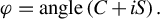 $$\begin{align}\varphi =\mathrm{angle}\left(C+ iS\right).\end{align}$$
The other barrier in the application of deep learning phase control is the non-unique phase-intensity mapping, which represents that different phase relationships may result in the same intensity distribution of the far field. Many solutions have been developed to solve the non-unique mapping problem, and one of the simplest, a diffractive pattern at a slightly defocused plane, is adopted here. In the simulation, all beams are assumed to be Gaussian fundamental mode and linearly polarized in the same direction. The intensity of the combined beam at the defocus far field can be expressed as follows:
 $$\begin{align}I\left(\boldsymbol{r},z=L\right)=\ &\frac{1}{i\lambda L}\exp \left(i\frac{\pi {r}^2}{\lambda L}\right) \mathrm{FT}\nonumber\\& \times \left\{\vphantom{\left[-{\left(\frac{\pmb{\rho} -{\pmb{\rho}}_{0n}}{w}\right)}^2\right]}\exp \left[i\frac{{\pi \rho}^2}{\lambda}\left(\frac{1}{L}-\frac{1}{f}\right)\right]\right.\nonumber\\& \left.\times\sum \limits_{n=0}^{N-1}A\exp \left[-{\left(\frac{\pmb{\rho} -{\pmb{\rho}}_{0n}}{w}\right)}^2\right]\exp \left(i{\varphi}_n\right)\right\},\nonumber\\[-10pt]\end{align}$$
where A, φ, w, $\pmb{\rho}_0 $
and λ are the amplitude, phase, waist width, central position and wavelength of the laser, respectively, and
$\pmb{\rho}_0 $
and λ are the amplitude, phase, waist width, central position and wavelength of the laser, respectively, and $\pmb{\rho} $
and
$\pmb{\rho} $
and $\boldsymbol{r} $
are the position vectors at the emission plane and observation plane while ρ and r of normal forms represent corresponding scalar distances from the origin. FT{·} refers to Fourier transform, and L and f represent the propagation length and the focus length, respectively (in our study, L ≠ f). It should be pointed out that the strategy of the defocus pattern is not contributed in this work, but it is important not only for solving the non-unique mapping problem but also for clarifying the optical model of dataset preparing. Therefore, the advantages of the strategies discussed in the following section correspond to the strategies of sin-cos loss and two-layer output, rather than the defocus pattern, since the training dataset is kept the same with or without strategies.
$\boldsymbol{r} $
are the position vectors at the emission plane and observation plane while ρ and r of normal forms represent corresponding scalar distances from the origin. FT{·} refers to Fourier transform, and L and f represent the propagation length and the focus length, respectively (in our study, L ≠ f). It should be pointed out that the strategy of the defocus pattern is not contributed in this work, but it is important not only for solving the non-unique mapping problem but also for clarifying the optical model of dataset preparing. Therefore, the advantages of the strategies discussed in the following section correspond to the strategies of sin-cos loss and two-layer output, rather than the defocus pattern, since the training dataset is kept the same with or without strategies.
2.3 Neural network construction
The VGG model, which is a powerful and prevalent tool in computer vision, is modified and employed as our neural network to achieve CBC phase control[ Reference Simonyan and Zisserman 44 ]. It is a classical convolution neural network, which consists of a series of convolution layers, max-pooling layers and fully connected (FC) layers, as shown in Figure 2. For simplicity, the network is divided into five blocks, and each block is made up of one or more convolution layers followed by a max-pooling layer. Based on the number of convolutional layers, VGG can be named VGG-11, VGG-13 and so on, and the one used in our study is VGG-16, including 13 convolution layers and three FC layers. The kernel size of all convolution layers is 3×3 and the padding size is 1, so the image height and width do not change after convolution, but the channel number might be different depending on the number of convolution filters. The kernel size of max-pooling layers is 2×2, so the image height and width will be reduced to the half after pooling. It should be noted that a rectified linear unit (ReLU) function is followed with each convolution layer and FC layer, which are not shown in the figure. A dropout layer with a possibility of 0.5 is added in both FC1 and FC2 to reduce the possibility of overfitting, and the activation function of FC3 is changed from softmax to sigmoid, as phase prediction is a regression problem rather than a classification problem.
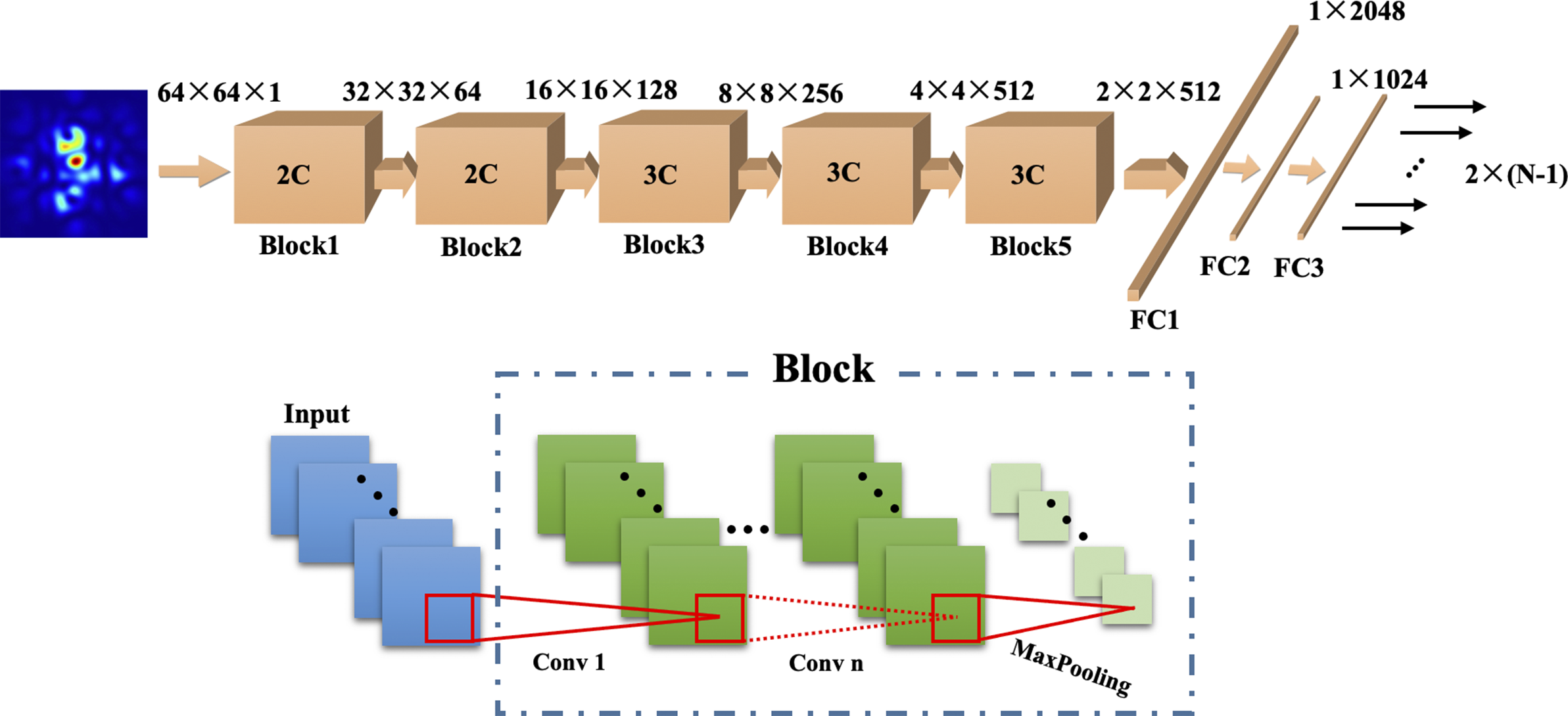
Figure 2 Structure chart of the VGG network.
The built VGG network can extract features of the input intensity profile by convolution operations layer by layer, and it can leave out redundant features by max-pooling layers to prevent overfit. In addition, the ReLU activation layers are beneficial to enhance the nonlinear expression ability of the network. After a series of convolution and max-pooling layers, the image features are efficiently extracted and condensed, and are flattened and reorganized by the FC layers. Finally, the output layer is formatted in size of 2 × (N – 1) while it is 1 × (N – 1) for traditional networks, so it maps these extracted features into the real and imaginary parts of a complex phase vector and achieves phase prediction consequently. To accommodate the phase-control tasks, the input image size of the VGG-11 model is changed to 64×64×1, and the intensity value is normalized with the maximal value being 1.
3 Results
3.1 Phase prediction with improved accuracy
The modified VGG-16 network for nine-channel CBC is built up and trained with 18,000 labeled data pairs. The batch size is 250 and the epoch is 90, and stochastic gradient descent with a momentum term is selected as the optimization algorithm, with a learning rate of 0.05 and momentum factor of 0.9. It takes less than 20 minutes for a personal computer to finish the training process. The calculated mean squared error (MSE) loss of 1000 testing samples at every epoch is plotted in Figure 3. The MSE loss drops from 1.0 at the start to 0.015 at the end, and it can be seen that the loss decreases very fast at the first five epochs and gradually becomes stable in the later epochs, illustrating that the network is convergent and the mapping from pattern to phase is constructed.
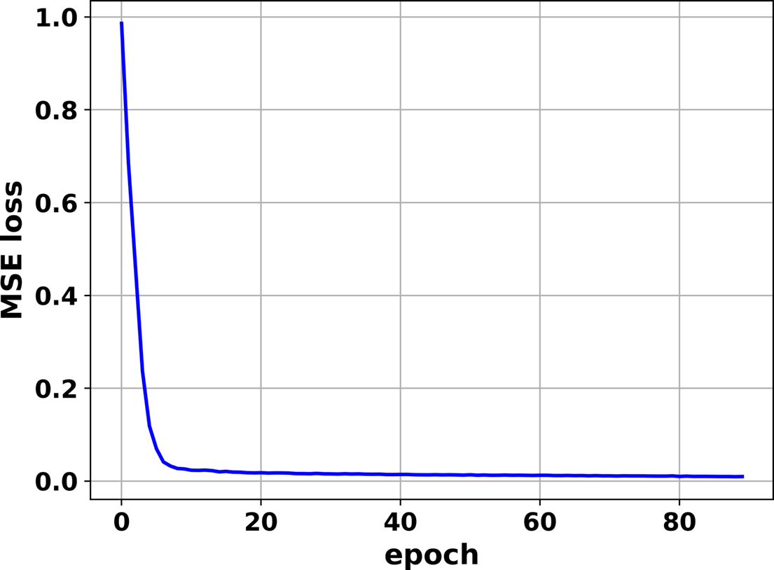
Figure 3 Testing loss with respect to the training epoch.
Then the trained network is validated on 1000 datasets that are not included in the training and testing process, and the phase predictions are compared with the true labels. Firstly, the root mean square (RMS) residual phase is introduced for quantitative analysis, which is calculated by the following:
 $$\begin{align}{\varphi}_{\mathrm{res}}=\frac{1}{N}\sum \limits_{n=0}^{N-1}{\left({\varphi}_n-\overline{\varphi}\right)}^2,\quad \overline{\varphi}=\frac{1}{N}\sum \limits_{n=0}^{N-1}{\varphi}_n.\end{align}$$
The RMS residual phase describes how well laser phases are synchronized, where a large value represents poor synchronization. The initial states of laser phases are quite different; the network predictions on samples of different initial states are shown in Figure 4, where the true phase and predicted phase of each beam are compared one by one (only eight beams are shown because one beam is used as the phase baseline). The initial RMS residual phases are 0.7, 1.2, 1.8 and 2.4 rad, respectively, the neural network makes precise predictions on these samples despite the initial conditions and no selectivity on beam position is observed. If predicted phases are used to compensate initial phases, phase-locking will be achieved in a single step, leading to RMS residual phases of λ/88, λ/83, λ/67 and λ/95 for the four samples, respectively.
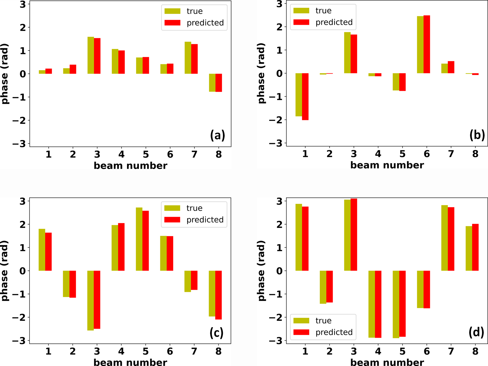
Figure 4 Predicted phase versus true phase for samples of different initial RMS residual phases: (a) 0.7 rad, (b) 1.2 rad, (c) 1.8 rad and (d) 2.4 rad.
Moreover, the phase prediction of each validation sample is calculated, and the compensated phase is equal to the initial phase minus predicted phase. The compensated phases of the 1000 validate samples with corresponding initial phases on each beam are plotted in Figure 5(a), where the dashed lines in the middle equal ±π/20, which is helpful to directly evaluate the prediction accuracy. The phase points in Figure 5(a) are gathered to a horizontal line with several slight ups and downs, and there are no isolated points far from the dashed area, indicating the network is capable of excellent phase prediction over the full phase range; thus, one-step phase control can be implemented no matter what the initial phases are. The RMS residual phase after one-step compensation averaged on the sample number is λ/95, which shows high prediction accuracy of our network. In addition, the same network is trained with the same dataset and same epochs using traditional MSE loss, and the phase compensation performance is as shown in Figure 5(b). It is obvious that the accuracy is much worse, especially when the initial phases are close to ±π, and the average residual phase after one-step control is only λ/12, showing the great advantages of the proposed training strategies.
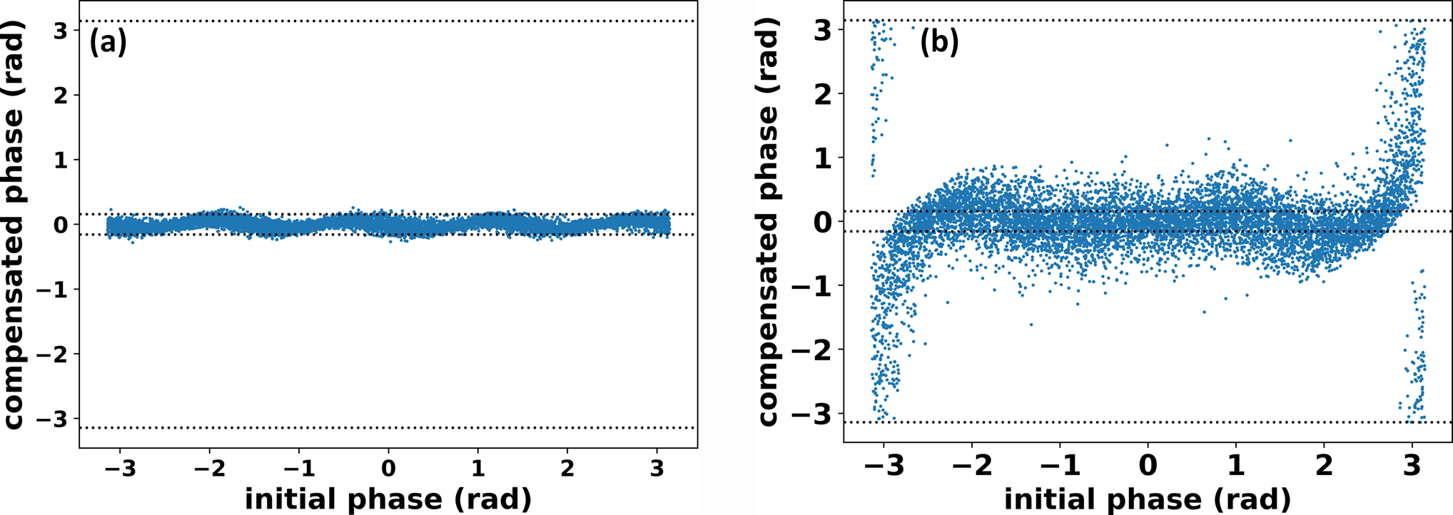
Figure 5 Prediction error as a function of true phase: (a) cos-sin loss and two-layer output and (b) traditional MSE loss and one-layer output.
3.2 Single-step phase control in filled-aperture system
Based on the trained neural network, single-step phase control is implemented in the filled-aperture CBC system with the assistance of delay control. The control procedure was described previously in Table 1 in detail, and the active control simulations are carried out in the entire phase and delay feedback loop. The parameters of the SPGD algorithm for delay control are optimized as γ = 0.6 and σ = 0.05, and the execution speed of deep learning phase control is set to be 10 times the delay loop, so the phases are locked when the delay controller acts and loop crosstalk will be avoided. The power in bucket (PIB) of the far-field pattern at the focus plane is calculated at each step to monitor the state of the sampled beam, and the PD signal intensity represents the combining efficiency of the whole system. The PIB and PD signal intensity during the process of phase delay are shown in Figure 6, where the x-label represents the delay control step. The drop-off lines in Figure 6(a) correspond to the voltage perturbations and updates of LCs, and combining efficiencies of both filled and tiled-aperture beams are maximized after around 35 steps. This result demonstrates that delay control is effective and single-step phase control for filled-aperture CBC is feasible.
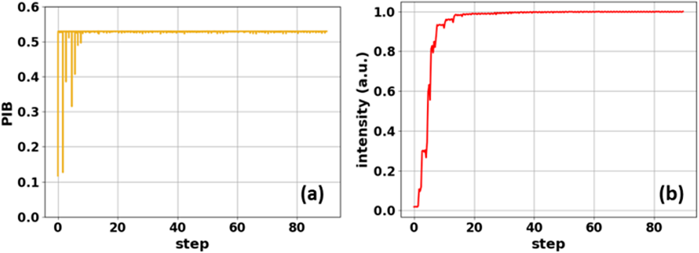
Figure 6 System state variation during delay control process: (a) PIB of the tiled-aperture combined beam and (b) normalized intensity of the filled-aperture combined beam.
Therefore, the phase relationships between tiled- and filled-aperture beams are synchronized after delay control, and phase control can be implemented directly in the filled-aperture CBC with delay value fixed. The delay residual after control of Figure 6 is λ/101 (converted to phase residual), which is small enough and is expected to have no significant impact on the control performance as the achieved combining efficiency is very close to 100%, as shown in Figure 6(b). This delay residual is considered in the simulation while the real-time delay control is turned off; the results of 20 random initial states are shown in Figure 7. One can clearly see that the system reaches the maximal intensity in a single step from any initial state. The combining efficiency is 98.7% and the residual phase is λ/70, which is limited by the delay control residual. Moreover, filled-aperture CBC is implemented by the traditional network as well and the combining efficiency over 20 random cases is 79.2% on average, showing great improvement brought about by the training strategies.
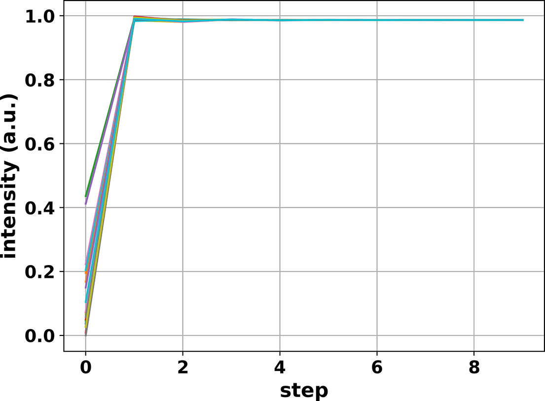
Figure 7 Single-step phase control of filled-aperture CBC.
As mentioned in Section 2.1, phase-control performance is critical for delay control, which will determine the feasibility of filled-aperture CBC by deep learning. Therefore, the requirement on phase prediction accuracy with application to filled-aperture CBC is investigated. A neural network with different prediction accuracy is obtained by varying training epochs, and the results are shown in Figure 8. It is apparent that the one-step phase residual decreases rapidly as training epochs increase, and the filled-aperture combining efficiency by using the neural network in cooperation with the delay controller becomes higher at the same time. For a typical efficiency of 95%, the one-step residual phase of the neural network should be better than λ/50.
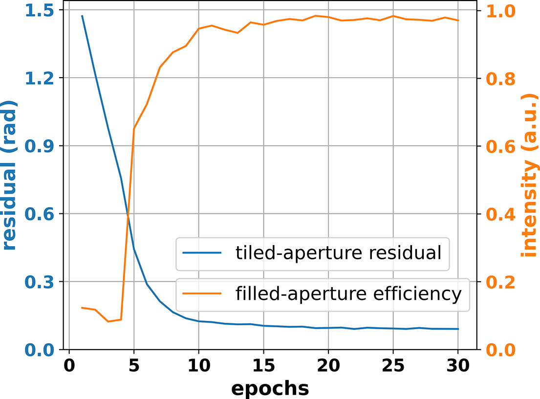
Figure 8 Single-step residual phase for filled-aperture CBC and combining efficiency for tiled-aperture CBC with respect to training epochs.
Another important issue is the dynamic phase perturbations that are commonly encountered in a real laser system. Bandwidth-limited white noise is introduced in the simulation model[ Reference Breitkopf, Eidam, Klenke, von Grafenstein, Carstens, Holzberger, Fill, Schreiber, Krausz, Tünnermann, Pupeza and Limpert 22 ], where the noise cut-off frequency is set to 100 Hz and RMS amplitude is λ/30. The time domain phase drift of one of the lasers is exemplified in Figure 9(a), and each laser experiences independent phase perturbations with the same cut-off frequency and RMS amplitude. The execution rate of the deep learning algorithm is set as 1 kHz (single-step time of 1 ms), and filled-aperture combining efficiency from open and closed loops is illustrated in Figure 9(b). With the control loop on, the combining efficiency rises immediately from less than 10% in the open loop to 96.7% in the closed loop. More specifically, the transition process at the moment of control turning on, as shown in Figure 9(c), manifests that phase-locking is achieved in a single step (1 ms) even with dynamic phase noise. Therefore, the dynamic phase noise does not affect the time convergence, but leads to a reduced efficiency loss (from 98.7% to 96.7%) and an increased residual phase (from λ/70 to λ/36). As the control loop takes actions at a step of 1 ms, the combining efficiency slowly drifts within the relaxation time before the next phase action is implemented. The power spectral density of phase noise of one laser, plotted in Figure 9(d), indicates that phase noise below 1 kHz is suppressed, and the control bandwidth of 1 kHz is achieved in a 1 kHz control loop thanks to the single-step advantage. It is predicted that the control bandwidth will be further improved by using a faster control loop.
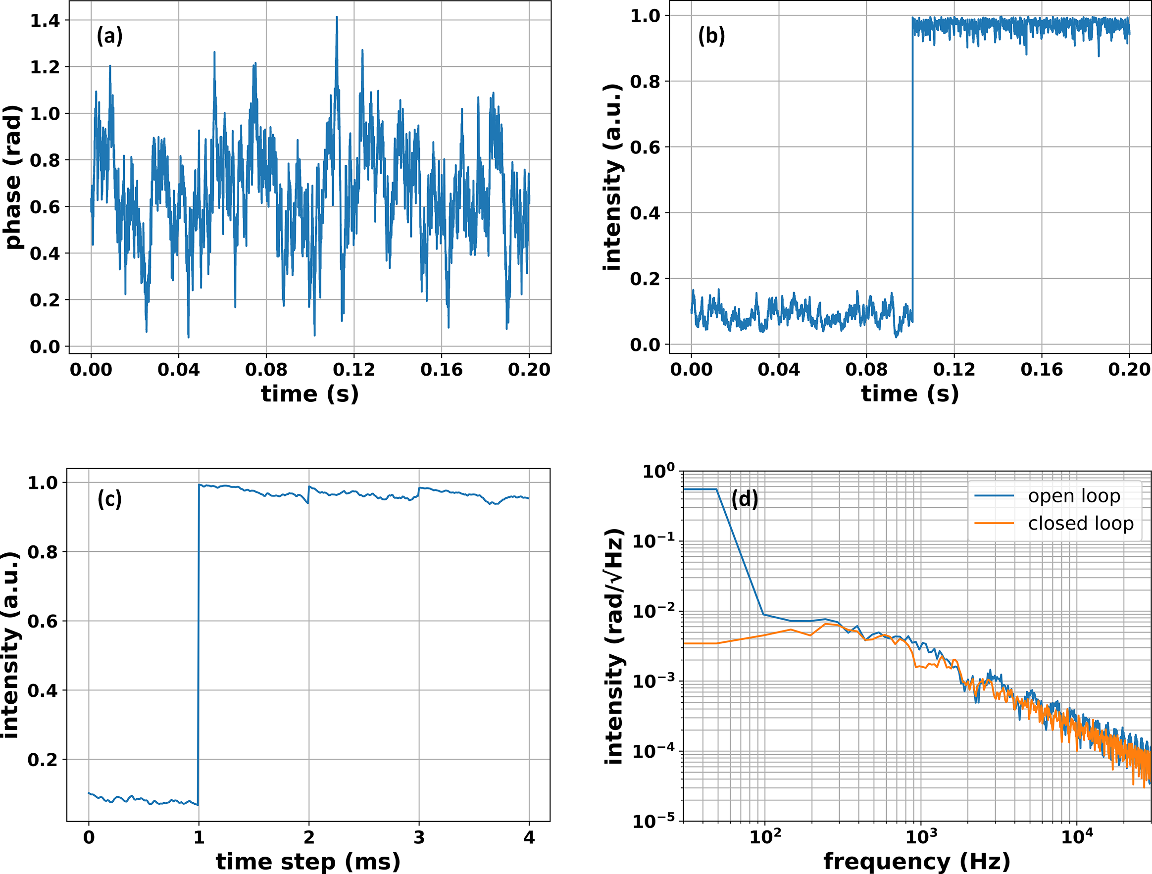
Figure 9 Filled-aperture CBC with dynamic phase noise: (a) time-dependent phase noise, (b) combining efficiency in open and closed loops, (c) time convergence detail from the open to the closed loop and (d) phase noise spectra in open and closed loops.
4 Discussion
One of the most attractive advantages of deep learning phase-control lines is that phase-locking can be achieved in a single step in spite of increasing channels. Indeed, phase-control performance highly depends on the residual phase or prediction error of the neural network, and previous studies showed decreasing accuracy with increasing channel number[ Reference Hou, An, Chang, Ma, Li, Zhi, Huang, Su, Wu, Ma and Zhou 37 ], so it is important to find out whether the channel number affects the residual phase in our models.
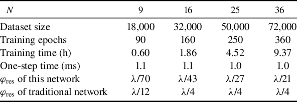
Neural networks for 9, 16, 25 and 36 beams are constructed and trained using the same strategies aforementioned, with a dataset size of 2000 times the beam number and training epochs of 10 times the beam number, as shown in Table 2. The network structure is VGG-16, as described before, but the output number is varied with the beam number. The average residual phases after one-step correction in filled-aperture systems with different channels are listed in Table 2. It is indicated that the residual phase increases as the channel scales, but the accuracy for a 36-channel CBC system is λ/21 and the combining efficiency is higher than 90%, which is acceptable for typical applications. In contrast, for a traditional network without using the proposed strategies, the one-step residual phase is about λ/4 for 16 or more channels, and the combining efficiencies are less than 5% for these cases. In the presence of dynamic perturbations (noise properties are the same as in the nine-channel case), filled-aperture CBC of 36 channels controlled by deep learning is simulated as well, and the results are shown in Figure 10. It is indicated that convergence speed is not affected by the dynamic noise, but the combining efficiency becomes worse in the closed loop, which is about 81%. In contrast, a neural network without training strategies is simulated as well, resulting in a combining efficiency of only 2%, showing no improvement by phase control. The other issue of concern is that the dataset size and training time rise rapidly with the channel number, as shown in Table 2, which is because the phase relationships and diffraction patterns become far more complicated. Specifically, if the laser phase is divided into p discrete pieces, such as p-values equally spaced in the range of [–π, π], the permutation and combination of N lasers will be pN , which means the problem dimension increases exponentially with channel number N. To acquire a higher accuracy, the number of phase pieces p should be larger, which will lead to a much larger dimension expansion rate. Therefore, the linearly increasing dataset size cannot catch up with the problem complexity, and thus the residual phase for a larger array becomes worse to some extent. In addition, the one-step time of network prediction, given in Table 2, shows that control speed is not affected by channel number, and the one-step time is close to 1 ms.
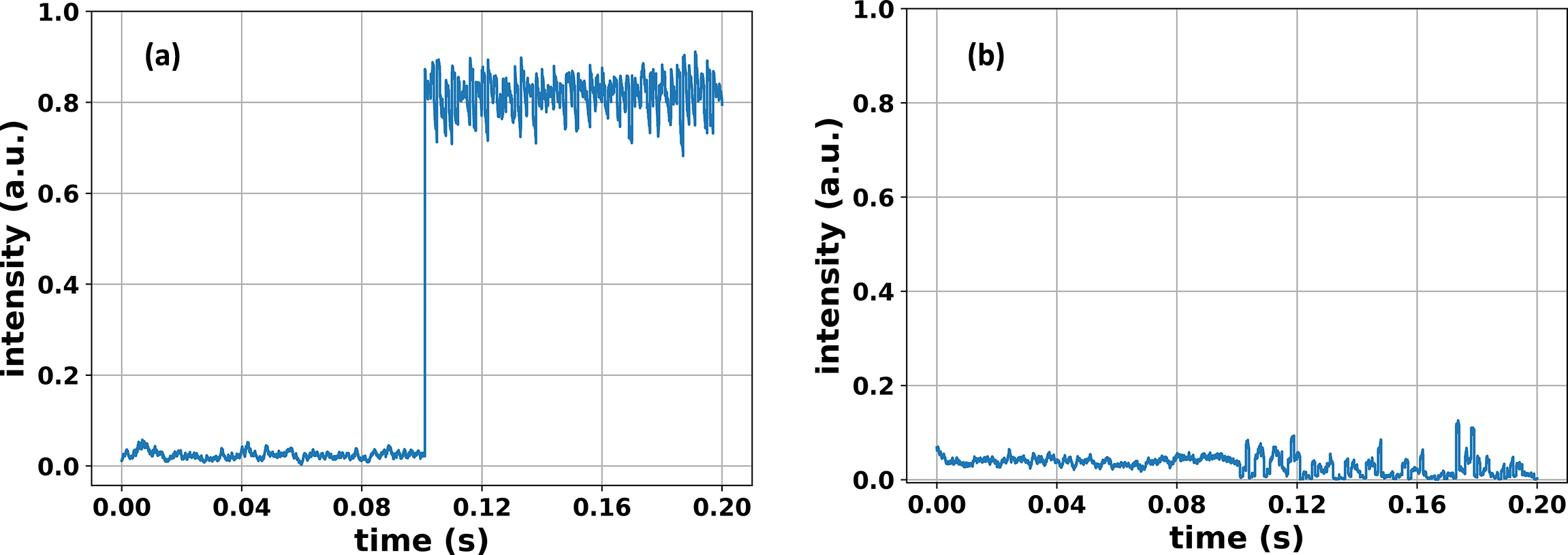
Figure 10 Filled-aperture CBC of 36 channels with dynamic phase noise. Phase control by deep learning (a) with and (b) without strategies.
Table 2 Residual phase after one-step phase control for different channel numbers.
In our simulation, the network is not optimized for different system scales, and it can be speculated that a smaller residual phase is possible at the price of a deeper and larger network and more effort on training. For instance, if the dataset size of 36-channel CBC is supplemented twice (144,000), the residual phase of filled-aperture control after one step will be improved to λ/29. Although more time and effort are spent in the network training for a larger array, the accuracy is still worse than in the nine-channel case. Therefore, to apply the method to a large-scale system, other phase-intensity mapping schemes, such as the sparsely sampled speckle pattern after a diffuser[ Reference Shpakovych, Maulion, Kermene, Boju, Armand, Desfarges-Berthelemot and Barthélemy 35 ], the diffraction pattern of a two-dimensional DOE[ Reference Wang, Du, Zhou, Li and Wilcox 34 ] and other innovative setups, are desirable to simplify the learning task so that a smaller network can be employed and the training process will be less intractable[ Reference Shpakovych, Maulion, Boju, Armand, Barthélémy, Desfarges-Berthelemot and Kermene 30 , Reference Wang, Du, Zhou, Gilardi, Kiran, Mohammed, Li and Wilcox 45 ]. In addition, the design and optimization of the dataset will probably make a difference since with randomly generated samples of limited size it is impossible to cover the problem space, and most samples will be far from the phase-locking state according to the statistical theorem. Therefore, the channel scalability of our method is related to the design of the optical mapping and network structure.
5 Conclusion
A deep learning algorithm for phase control of filled-aperture CBC is proposed and verified in a nine-channel system. By accommodating the mapping problem of pattern to phases, the modified neural network employing strategies of sin-cos loss and complex output yields single-step phase compensation with residual phase error as low as λ/95. The modified deep learning algorithm is then applied to the filled-aperture phase control assisted by delay control, and phase-locking can be achieved in a single step, resulting in a residual phase of λ/70. Furthermore, the scalability and performance under dynamic phase perturbations of deep learning phase control are discussed, and the results can offer a promising solution to bandwidth improvement for filled-aperture CBC.


 Open access