2 Beamline setup and free run analysis

The experimental setup at the petawatt BELLA laser facility is illustrated in Figure 1 ^[ Reference Nakamura, Mao, Gonsalves, Vincenti, Mittelberger, Daniels, Magana, Toth and Leemans ^{10 ]}. The BELLA laser can deliver over 40 J of infrared energy per pulse at 800 nm in about 30 fs, achieving a peak optical power exceeding 1.3 PW at a repetition rate of 1 Hz. The system starts with a front-end low-power seed laser operating at 1 kHz. This beam is then passed through a series of amplifiers powered by 1 Hz pump lasers, producing an amplified 1 Hz beam along with an unamplified 1 kHz pilot beam.

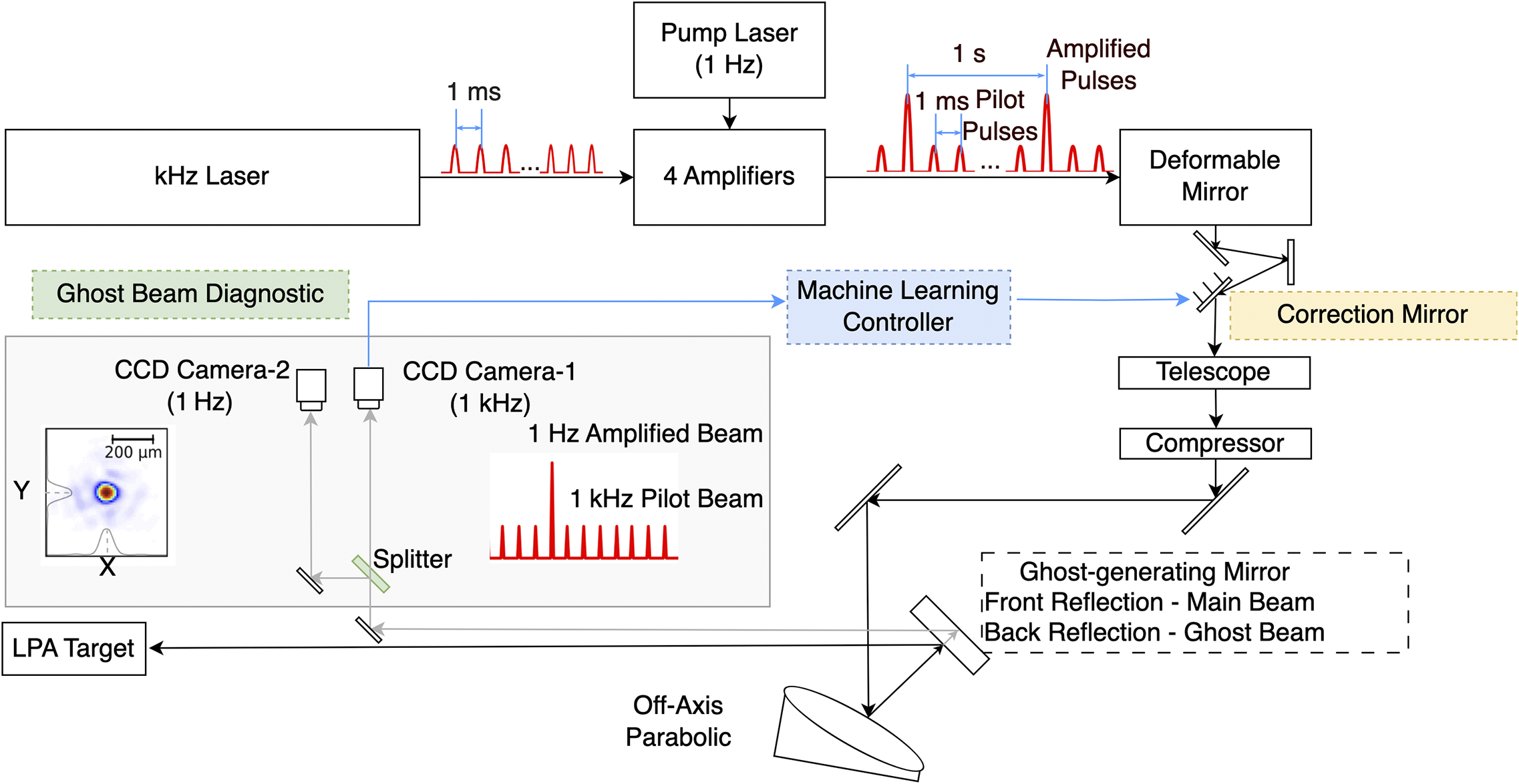
Figure 1 Schematic of the BELLA PW laser system, including the pilot beam diagnostics, correction mirror and focus optics. The setup enables high-resolution monitoring and control of the amplified laser beam.

In the laser amplification chain, there is a telescope between each stage to expand the beam size as the energy increases, maintaining fluence lower than the optics’ damage threshold. The beam size is 70 mm in diameter after the amplifiers and before the compressor.

After amplification, the beam is reflected from a deformable mirror and the ‘correction mirror’, which is used to make fine adjustments to beam pointing. It is the last mirror that can be used for correction; this mirror, actuated with piezoelectric transducers, is controlled to correct pointing at the target. Its dimensions are 100 mm $\times$ 150 mm, using commercially produced mount (4 inches $\times$ 6 inches) with closed-loop controls inside, driving an S-340 Piezo Tip/Tilt Platform^{[ 17 ]}.

The beam is then expanded in a telescope before it enters an adjustable pulse compressor, which allows fine-tuning of the laser pulse duration. After the telescope, the beam diameter is 210 mm (8.27 inches), transported with mirrors of 12–19 inches diameter, which are too heavy to control.

The laser beam is then directed to an OAP mirror, with focal length of 13.5 m, which focuses it to a spot size of approximately 50–60 $\unicode{x3bc} \mathrm{m}$ FWHM. After the OAP, there is a ghost-generating mirror 14 inches in diameter and 2 inches in thickness. The second surface of this ghost-generating mirror is coated for high reflection, providing a ‘ghost’ beam with enough intensity for the position sensing cameras. The ghost beam diagnostics setup, shown in the inset of Figure 1, includes a 50:50 beamsplitter that creates two copies of the ghost beam for two measurements.

The reflected ghost beam is directed to two charge-coupled device (CCD) cameras triggered at 1 Hz and 1 kHz. The former is used to monitor the position at the focus of the main amplified pulse and the latter to provide the data for ML-based stabilization.

We have found that the pilot beam is highly correlated with the petawatt amplified beam, as both traverse the same optical paths^[ Reference Berger, Barber, Isono, Jensen, Natal, Gonsalves and van Tilborg ^{3 ,} Reference Isono, van Tilborg, Barber, Natal, Berger, Tsai, Ostermayr, Gonsalves, Geddes and Esarey ^{12 ]}. The 1 kHz pilot beam enables the analysis and the precise monitoring of high-frequency errors, ensuring that noise up to 500 Hz is effectively measured for system diagnostics and performance optimization.

Analyzing system data is essential for control modeling, especially for developing data-driven ML solutions. Figure 2(a) shows the beam position data for both the x- and y-axes over a 35-h free (unstabilized) run without any existing feedback that can move the long-term slow drift. In this figure, each point represents the average centroid position. The system stability is quantified by the RMS deviation of the centroid positions, providing a clear measure of position error over time. A slow drift can be observed in the average centroid curves for both the x- and y-axes, indicating gradual changes in laser alignment over time. We include an inset in Figure 2(a) showing a 10-min segment of the 1 Hz beam position data in both the x and y directions. This inset highlights the rapid, short-term shot-to-shot fluctuations that are superimposed on the slower drift. Here, we focus on short-term laser position instability, or shot-to-shot jitter, as illustrated in the inset plot, rather than long-term drift, which is low frequency and can be mitigated by slow, existing active feedback systems. The average short-term instability, calculated as the mean of the 34 data points (one data point per hour), shows the average instability of ${\sigma}_{x,\mathrm{free}} = 10.15\;\unicode{x3bc} \mathrm{m}$ and ${\sigma}_{y,\mathrm{free}} = 11.82\;\unicode{x3bc} \mathrm{m}$ . It is typical for the x-axis to exhibit slightly better stability than the y-axis in the BELLA system, as well as in other high-power lasers^[ Reference Xu, Lu, Li, Wu, Li, Wang, Li, Lu, Liu, Leng, Li and Xu ^{18 ,} Reference Zhang, Wu, Hu, Yang, Gui, Ji, Liu, Wang, Liu, Lu, Xu, Leng, Li and Xu ^{19 ]}. This discrepancy can be attributed to greater vertical (y-axis) vibration of optical mounts in response to ground vibration.

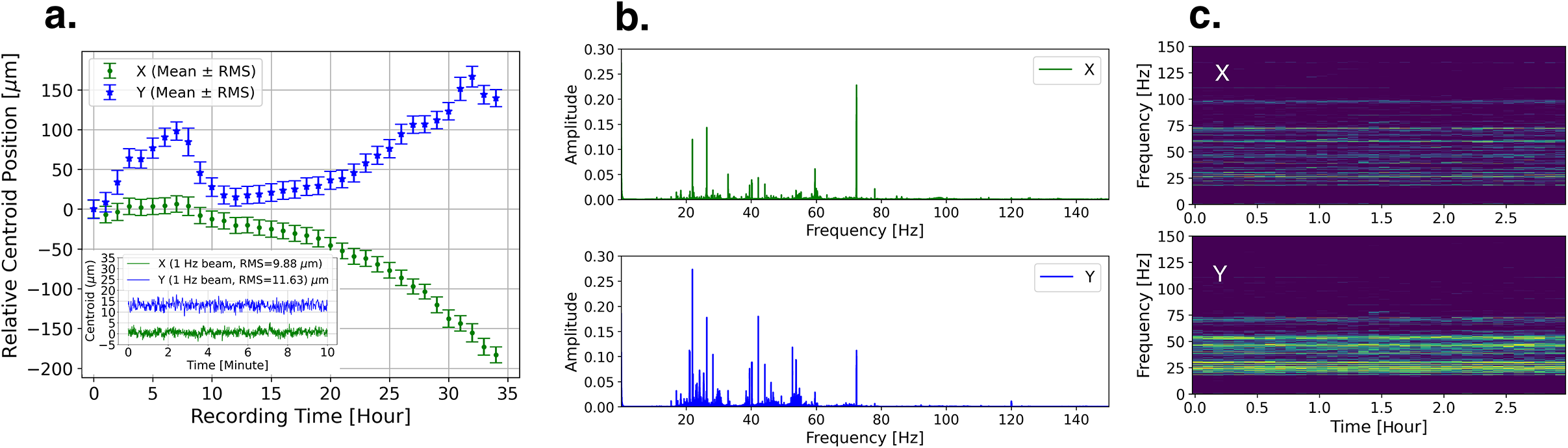
Figure 2 Free run noise analysis of the PW beamline. (a) Centroid position of the pilot beam over 35 h showing long-term drift. (b) Fourier analysis of noise frequency components in the x and y directions based on a 10-min subset of centroid data from the 1 kHz pilot beam. (c) Temporal evolution of frequency components over 3 h.

Figure 2(b) displays a typical spectrum obtained through Fourier analysis of a 10-min subset of centroid data from the 1 kHz pilot beam, providing a frequency-domain view of noise characteristics. The results show that the predominant frequency components for both the x- and y-axes are in the tens of hertz range. The horizontal axis (x) exhibits a simpler frequency profile compared to the vertical axis (y), which shows a broader range of frequency components between 20 and 60 Hz, along with an additional peak at 120 Hz. This greater complexity in the y-axis data explains why ML models with training processes tend to perform better in predicting the behavior of the x-axis.

Figure 2(c) further illustrates how the frequency spectrum evolves over a 3-h period, showing the temporal variations in noise frequency components derived in Figure 2(b). This short-time Fourier transform analysis highlights transient changes and periodic noise behavior, helping one to understand fluctuations over time. The data presented here provide a comprehensive assessment of both the spatial and temporal noise characteristics, which is crucial for developing control models, as a foundation for offline training and testing of ML algorithms.

3 Machine learning control diagram

The main limitation on feedback control loop bandwidth is primarily due to the inertia of the correction mirror (100 mm $\times$ 150 mm) shown in Figure 1. The mirror assembly includes its own PID (proportional–integral–derivative) controller, which is operated through an external setpoint.

Our previous work^[ Reference Berger, Barber, Isono, Jensen, Natal, Gonsalves and van Tilborg ^{3 ]} on a similar setup, the HTU, demonstrated stability improvements using a commercial feedback controller (ALIGNA-4D provided by TEM Messtechnik) ope rating at 1 kHz. Reference [Reference Genoud, Wojda, Burza, Persson and Wahlström8] also shows the effectiveness of active stabilization based on the traditional feedback system.

While both Refs. [Reference Berger, Barber, Isono, Jensen, Natal, Gonsalves and van Tilborg3] and [Reference Genoud, Wojda, Burza, Persson and Wahlström8] show long-term and shot-to-shot oscillation suppression, they highlight the fundamental bandwidth limitations of PID-based feedback due to hardware constraints^[ Reference Franklin, Powell, Emami-Naeini and Powell ^{20 ]}. In particular, Ref. [Reference Berger, Barber, Isono, Jensen, Natal, Gonsalves and van Tilborg3] reported that a large 4-inch correction mirror resulted in a measured feedback bandwidth of only 20 Hz. We measured the performance of a commercially available stabilizer, the Aligna system, at the BELLA HUT facility. The resulting spectrum clearly demonstrates that the Aligna system suppresses frequency components primarily in the 10–20 Hz range. This behavior is consistent with the known bandwidth limitations of traditional feedback control systems. However, Figure 2(b) shows that our laser system exhibits significantly higher frequency components beyond 20 Hz, presenting a major challenge for implementing traditional feedback control effectively. This challenge is further exacerbated by our specific setup, which uses a large 4-inch by 6-inch correction mirror – making it even more susceptible to bandwidth limitations – and serves as a key motivation for the new approach presented in this work.

ML is a widely considered a valuable approach in time-series forecasting topic, which includes prediction of laser pointing oscillation. The control system diagram is shown in Figure 3. In this feedback loop, ML is employed to predict the behavior of the 1 Hz/PW laser based on information from the 1 kHz pilot signal captured by the ghost beam diagnostic camera. This allows the controlled mirror to be repositioned in advance, effectively compensating for any predicted errors and enabling shot-to-shot stabilization of the 1 Hz/PW beam.

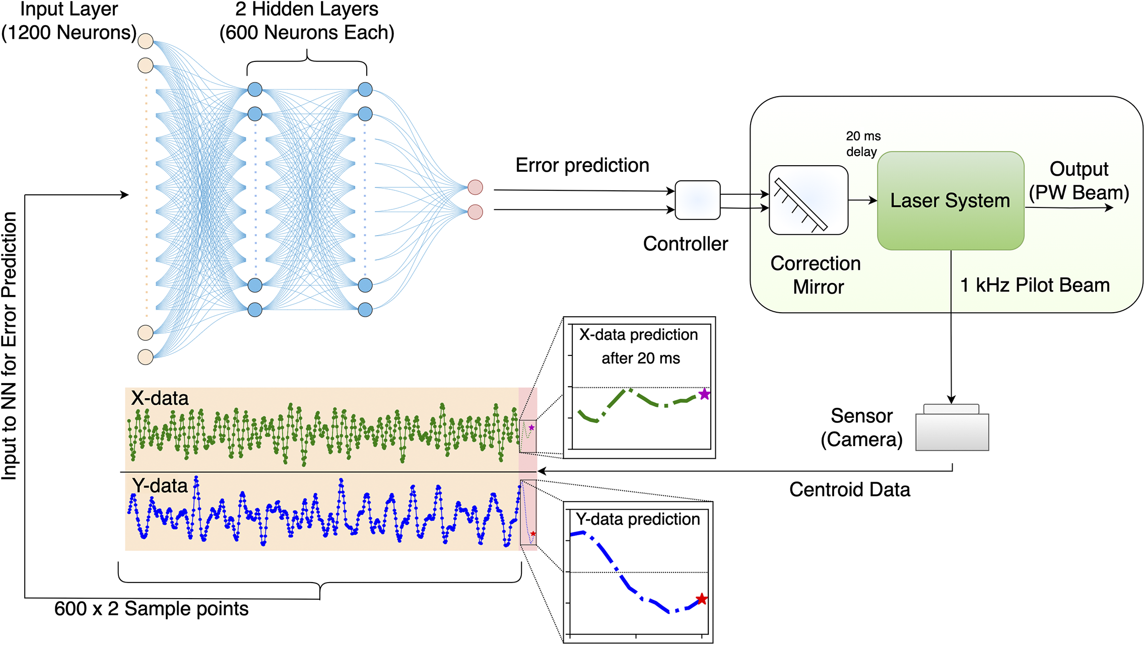
Figure 3 Machine learning control diagram: machine learning feedback loop for predictive control of the BELLA PW laser. The model uses pilot beam data to adjust the correction mirror preemptively, compensating for system noise.

The standard feedback method using a 1 kHz pilot beam relies on a simple PID controller, which treats the 1 kHz beam data as the error signal for correction. However, due to the slow response of the mirror (20 ms), the error signal used for correction does not reflect the actual system error when the mirror reaches the corrected position. This 20 ms delay (illustrated in the zoomed-in plots in Figure 3) limits the PID controller to correcting slow drifts, but it makes it incapable of addressing high-frequency components in the shot-to-shot jitters. In the frequency domain, the mismatch between the correction signal and the actual error 20 ms later is primarily influenced by the disturbance frequency sources shown in Figure 2. With a control bandwidth limitation (referenced in Ref. [Reference Natal, Barber, Isono, Berger, Gonsalves, Fuchs and van Tilborg13]), the PID controller cannot address high-frequency system errors, unlike our ML approach, which is not constrained by such bandwidth limitations.

We evaluated several ML models with different neural network architectures, including long short-term memory (LSTM) networks, simple recurrent neural networks (RNNs), and multi-layer perceptrons (MLPs). LSTM networks are specialized for handling sequential data, such as time series, by learning long-term dependencies and effectively capturing patterns over extended periods. Simple RNNs, while similar, have a more basic architecture and are typically used for shorter sequences due to their limitations in retaining long-term memory. MLPs, in contrast, are traditional feedforward networks consisting of multiple layers of nodes where each layer is fully connected to the next. Although MLPs are generally used for non-sequential data, our study found that they performed comparably to RNNs and LSTM networks on sequential data after appropriate preprocessing and feature engineering. This indicates that MLPs, with the right data preparation, can effectively capture essential patterns in sequential datasets.

The simpler structure of MLPs can be advantageous in terms of computational efficiency and ease of implementation, especially when real-time performance is crucial. The choice of MLP model is driven by its simplicity and ease of integration into a field-programmable gate array (FPGA)-based control loop, which is critical for achieving precise timing in future applications. An important observation from our study is that proper scaling of the training data is essential; the training data must reflect the range of values expected during the testing and correction phases. Hyperparameters refer to the configuration settings of an ML model that are not learned from the data during training but are set before the learning process begins. Examples of hyperparameters include the number of neurons in a neural network layer, the learning rate and the number of training epochs. Tuning these parameters is necessary for optimizing the model’s performance.

The chosen layout of the MLP model has 1200 neurons in the input layer (accounting for $600\times 2$ sample points for both the x- and y-axes) and two hidden layers with 600 neurons, optimized through hyperparameter tuning using Optuna^[ Reference Akiba, Sano, Yanase, Ohta and Koyama ^{21 ]}. This configuration provides a robust and efficient solution for the control loop, balancing performance and implementation complexity.

The input to the ML model consists of sequential data from the 1 kHz pilot beam in both the x and y directions. The ‘input window’ refers to the duration of data used for making predictions. In our setup, the input window is 600 ms, but this duration can be adjusted as needed. The ‘delay time’ is the interval between the last sample point in the input window and the prediction point, which is the arrival time of the PW pulse. The delay time depends on the response time of the controller mirror. For our system, the delay time must be at least 20 ms to ensure the mirror has enough time to reach a stable position. In our case, for the first corrected PW beam, with a delay time of 20 ms and an input window of 600 ms, we collect data from 380 to 980 ms (within a cycle length of 1000 ms). The data are then used to make predictions and adjust the mirror position. After 20 ms, the mirror reaches the desired position, correcting the system noise just as the 1 Hz PW beam is delivered to the target.

We have conducted a comprehensive study on the effects of varying the input window and delay time in the simulation described in Section 4. This analysis helps to determine the optimal values for these parameters, ensuring the precise timing and accuracy needed for effective system noise compensation.

4 Simulation results

We present ML predictions versus the actual measured values for the focused PW beam position over a 20-min period, as shown in Figure 4(a). This 20-min timeframe includes a total of 1200 pulses, which allows for direct comparison between the experimental recordings and the predicted values. The ML model was trained using data from a 100-s pilot beam run, yielding 100,000 data points in total. To optimize sample collection, we applied a sliding window technique to generate a sufficient number of training samples. Specifically, we labeled the centroid positions from $i$ to $i+599$ ms as the input, combined the x and y coordinates into a single array, and labeled the centroid position at $i+619$ ms as the output to predict. Using this labeled data, the ML model learned the relationship between the input and output in a supervised learning framework.

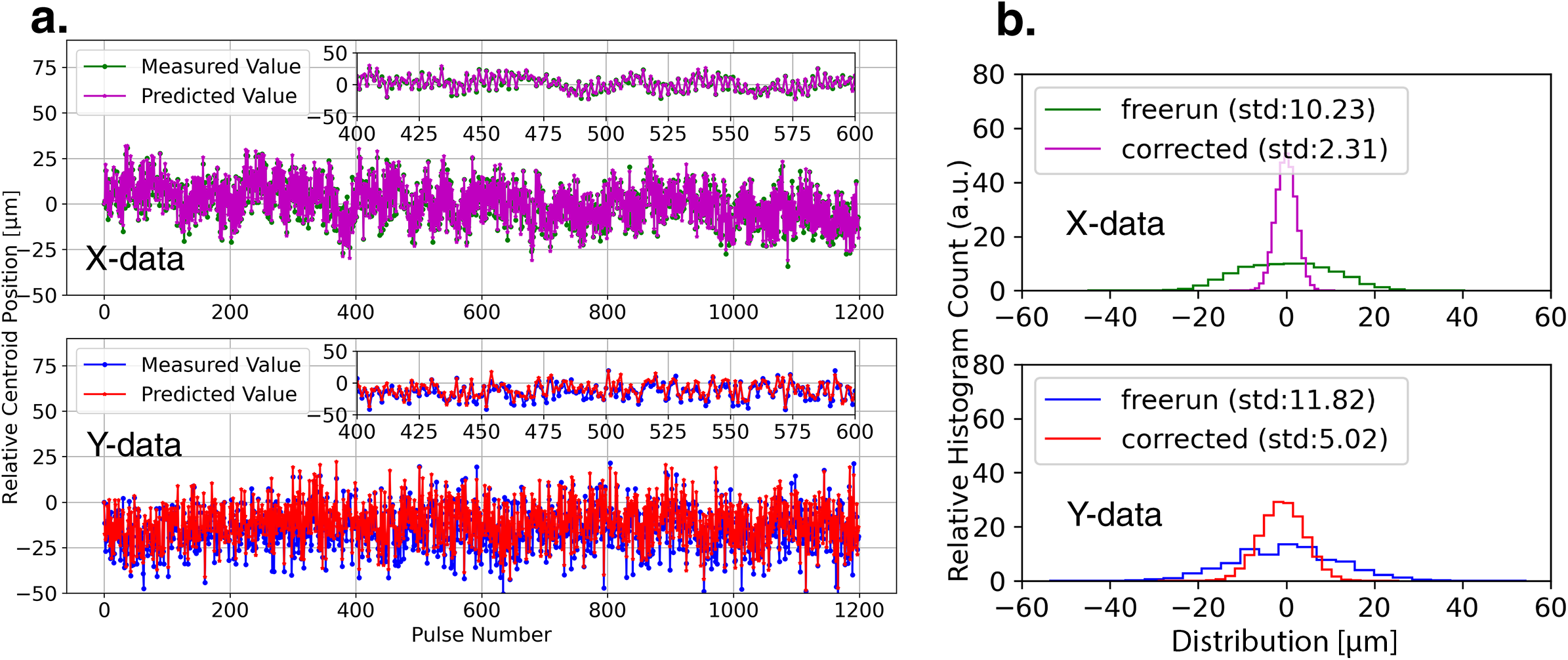
Figure 4 The simulation results show one case of ML model predictions versus measured centroid values for the PW beam, given the dataset of 20 min (1200 data points) of a 1 Hz beam from Figure 2(a). (b) Statistics of the 1200 data points before and after ML correction show jitter reduction of 77.4% in the x direction and 57.5% in the y direction, demonstrating the model’s effectiveness in simulated conditions.

Then, for testing, we used data collected from 380 to 980 ms in each pulse cycle as input to predict the centroid position at the end of the pulse cycle, which occurs every second. This approach allowed us to evaluate the model’s ability to predict the centroid position for each 1 Hz PW pulse. The results showed a strong agreement between the ML predictions and the actual measured values, demonstrating the accuracy of the ML model in offline testing.

The remaining error after correction is calculated as the difference between the predicted and actual values. To evaluate the effectiveness of the ML model, we compared the centroid positions before and after ML correction to determine the error reduction percentage. This percentage is calculated as the difference between the free run (uncorrected) and corrected RMS values, divided by the free run RMS value. In our case, as shown in Figure 4(b), we achieved an error reduction of 77.4% in the x direction and 57.5% in the y direction.

Figure 5 shows the results of a parameter scan. Figure 5(a) illustrates how the input window (the number of sample points in the x and y dimensions) affects control performance, while Figure 5(b) demonstrates the influence of delay time caused by the lag in mirror response. The analysis is based on the PW beamline data shown in Figure 1 and utilizes the control model depicted in Figure 3. From a learning perspective, increasing the duration of the ‘input window’ provides the ML model with more time-series information, improving prediction accuracy until the input data contains sufficient information, at which point accuracy saturates. Conversely, shorter ‘delay times’ make it easier for the ML model to predict trends, also enhancing accuracy. The optimal values for these parameters depend on the specific system characteristics, as illustrated by the information in Figure 2. We conducted training and testing across various datasets collected over different time periods, calculating the centroid positions before and after ML correction to assess the percentage reduction in position error.

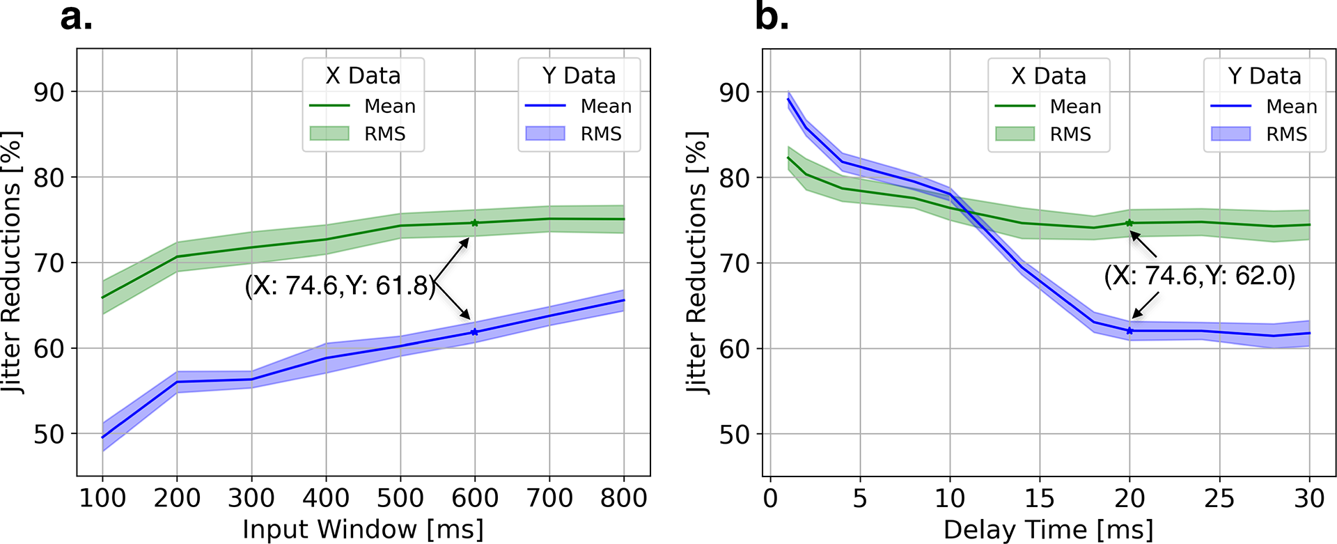
Figure 5 Simulation on a parameter scan with 10 h of data (datasets are the same as in Figure 2): examining the impact of (a) input window and (b) delay time on control performance. Results using experimental parameters (input window of 600 ms and delay time of 20 ms) indicate the average reduction in jitter is 75% in the x direction and 62% in the y direction.

We evaluated 10 datasets, each representing 1 h of data (the same as in Figure 2). For each of these 10 h, we calculated the mean and RMS values for statistical analysis. The results align with our expectations and reveal several key observations. (1) Both the x- and y-axes exhibit improved performance with a longer input window and a shorter delay time, highlighting the importance of using an adequate amount of time-sequential data for accurate predictions. (2) The x-axis outperforms the y-axis in terms of control precision, likely due to its simpler dynamics, which make it easier to model and predict. (3) Although the delay time is generally fixed for a specific mirror configuration, there is potential to fine-tune this parameter using advanced timing and synchronization systems, which could enable corrections even before the mirror reaches full stabilization. We plan to investigate this approach further using FPGA technology in future studies. (4) For our experiment, the optimal parameters considering both accuracy and calculation latency were an input window of 600 ms and a delay time of 20 ms, which resulted in an error reduction of 74.6% for the x-axis and approximately 61.8%–62.0% for the y-axis. The consistent performance improvement in the x-axis and the minor variations in the y-axis indicate a reasonable level of randomness in the ML training process and underscore the robustness of our method.

To further compare our ML-based method with the traditional Aligna system implemented at the BELLA HTU setup, we have included additional data shown in Figure S2-2 of the Supplementary Material. This figure presents the centroid distribution from the 1 Hz HTU data, comparing the experimental results with the Aligna system off and the Aligna system on, and the simulated ML-based correction. The simulated ML-based stabilization demonstrates comparable performance to our observations, reducing the standard deviation from $\sigma$ = 0.65 pixels to $\sigma$ = 0.23 pixels – a reduction of approximately 65%. The improved performance of the simulated ML-based approach compared to the Aligna system on ( $\sigma$ = 0.37 pixels) further underscores the motivation for pursuing this method.

5 Experimental results and discussion

Experimental results, presented in Figure 6(a), show the effectiveness of our approach over a recording period of approximately 1 h, consisting of 30 min of free run operation followed by 30 min of ML correction. During the free run period, the RMS jitter in the x direction was approximately 13.1 $\unicode{x3bc} \mathrm{m}$ , and in the y direction, it was around 14.8 $\unicode{x3bc} \mathrm{m}$ . With ML correction enabled, we observed a drop of the RMS values to 4.6 $\unicode{x3bc} \mathrm{m}$ in the x direction and 7.9 $\unicode{x3bc} \mathrm{m}$ in the y direction. This corresponds to jitter reductions of 64.9% in the x direction and 46.9% in the y direction.

Figure 6 Experimental validation. (a) Comparison of free run and ML-corrected jitter over 1 h in the time domain. (b) Centroid distribution in the two-dimensional (2D) x–y plane compared with the focused laser beam spot as background, in which each dot is the centroid of each pulse. The ellipses represent the $\sigma$ of each distribution.

Figure 6(b) shows the measured results in terms of shot-to-shot error compared with the beam size, with the focal spot displayed as a red background. The raw image of the focal spot is also shown in Figure S3 of the Supplementary Material. The centroid distribution is plotted on top of this image as blue dots (free run) and white dots (corrected). In addition, the plot shows the 3 $\sigma$ ellipse representing the beam size (red curve), the 3 $\sigma$ ellipse for the free run centroid distribution (blue curve) and the 3 $\sigma$ ellipse for the corrected centroid distribution (white curve). The standard deviation values, labeled as $\sigma$ , are provided in the plot legend. For the free run case, the jitter-to-beam-size ratio in the x-direction is $13.1\kern0.22em \unicode{x3bc} \mathrm{m}/25.2\kern0.22em \unicode{x3bc} \mathrm{m}\ (0.52)$ , and in the y-direction, it is $14.8\kern0.22em \unicode{x3bc} \mathrm{m}/24.4\kern0.22em \unicode{x3bc} \mathrm{m}\ (0.61)$ . After applying ML correction, the ratio in the x-direction is reduced to $4.6\kern0.22em \unicode{x3bc} \mathrm{m}/25.2\kern0.22em \unicode{x3bc} \mathrm{m}\ (0.18)$ , and in the y-direction, it becomes $7.9\kern0.22em \unicode{x3bc} \mathrm{m}/24.4\kern0.22em \unicode{x3bc} \mathrm{m}\ (0.32)$ . Although the reduction percentage results are slightly lower than those predicted by simulations, this discrepancy is likely due to additional sources of error, such as communication delays between the central processing unit (CPU) and hardware, which make precise timing difficult to achieve.

This is the first instance of shot-to-shot pointing error reduction beyond the bandwidth limitations typical of non-predictive control. The final errors of 4.6 $\unicode{x3bc} \mathrm{m}$ in the x direction and 7.9 $\unicode{x3bc} \mathrm{m}$ in the y direction correspond to angular deviations at the OAP focusing mirror of 0.34 $\unicode{x3bc} \mathrm{rad}$ in the x direction and 0.59 $\unicode{x3bc} \mathrm{rad}$ in the y direction, given the OAP focal length of 13.5 m.

The laser energy used in Figure 6 is amplified but not fully, reaching around 30 mJ. This serves as a proof-of-principle for the entire system closed-loop correction. We plan to apply this correction method in future high-energy (30 J) LPA experiments, with a timeline integrated into the beamline schedule. This ML-based approach is also scalable to setups with additional mirrors. Our future work will involve implementing pointing stabilization at the LPA target, utilizing two mirrors for angle corrections.