


1. Introduction
Nominally two-dimensional (2-D) surface irregularities in the form of backward-facing steps (BFSs), forward-facing steps and gaps have been a long-standing topic of interest in both theoretical research and engineering fields. Supersonic BFS flow represents a canonical case for the study of flow separation, which also occurs in many engineering applications, such as flame stabilization and supersonic mixing. Although the geometry is simple, the flow structure behind the step is not, particularly in the supersonic flow regime. Such flow is usually characterized by expansion waves, lip and reattachment shock waves, and a recirculation zone beneath a shear layer, which make supersonic BFS attractive for fundamental research of various flow physics. However, many studies have focused on incompressible BFS flow, leaving the complex flow physics in the supersonic flow regime unclear. The main motivation of the present study is to establish a primary understanding of global instability in supersonic BFS flow.
Numerous investigations have been carried out to understand subsonic BFS flow features through computational and experimental methods, which provide a relatively abundant understanding of various flow phenomena, including convective and intrinsic instabilities. The Kelvin–Helmholtz (K–H) instability, which is introduced by the shear layer generated by the separation region, is one of the most well-known convective instabilities in subsonic BFS flow, and it has mostly been studied at rather large step heights. To date, there have been considerable experimental and numerical studies that show evidence of K–H instabilities in subsonic BFS flow (Hasan Reference Hasan1992; Rani & Sheu Reference Rani and Sheu2006; Rani, Sheu & Tsai Reference Rani, Sheu and Tsai2007; Schäfer, Breuer & Durst Reference Schäfer, Breuer and Durst2009; Schröder et al. Reference Schröder, Schanz, Heine and Dierksheide2013; Bolgar, Scharnowski & Kähler Reference Bolgar, Scharnowski and Kähler2018; Eppink Reference Eppink2022). Kaiktsis et al. (Reference Kaiktsis, Karniadakis and Orszag1991) found that the BFS flow with an expansion ratio of  $\varGamma $= 0.5 (i.e. the ratio of the step height to the channel height downstream) was convectively unstable to the K–H instability at Re = 525 (Re is based on half of the downstream channel height and the maximum incoming velocity on the centreline) in a large portion of the flow domain using local stability analysis based on the parallel-flow assumption. Note that their geometry is different from that in figure 4. Nowruzi, Salman Nourazar & Ghassemi (Reference Nowruzi, Salman Nourazar and Ghassemi2018) adopted an energy gradient method to study the convective instability of subsonic BFS flow under different Reynolds numbers and expansion ratios, and concluded that the onset of instability originated in the separated shear layer. A prevailing viewpoint suggests that the dynamic processes observed in such subsonic BFS flow, particularly the oscillations of separated shear layers, arise from the presence of vortical structures known as K–H vortices. At higher Reynolds numbers, these K–H vortices become increasingly prominent and influential in shaping the flow patterns and dynamics within the shear layer. As these vortices are convected downstream, they induce significant alterations to the overall flow structure. Another focus of research is the step's potential to destabilize Tollmien–Schlichting (T–S) waves. As the entering T–S waves develop, especially in flows with higher Reynolds numbers, a combined instability mechanism with K–H instability downstream of the step can occur (Wang & Gaster Reference Wang and Gaster2005; Eppink et al. Reference Eppink, Wlezien, King and Choudhari2018; Crouch & Kosorygin Reference Crouch and Kosorygin2020). Recently, Hildebrand et al. (Reference Hildebrand, Mysore, Choudhari, Venkatachari and Paredes2022) performed a linear stability analysis of a BFS flow without the confinement of the upper wall and found that the growth rate of the T–S wave significantly increased in the separation region. K–H instabilities can also be distinguished in direct numerical simulation (DNS) with a turbulent inflow in internal BFS flows (Le, Moin & Kim Reference Le, Moin and Kim1997a; Barri et al. Reference Barri, El Khoury, Andersson and Pettersen2010; Pont-Vílchez et al. Reference Pont-Vílchez, Trias, Gorobets and Oliva2019). Moreover, temporal transient growth analysis was performed by Blackburn, Barkley & Sherwin (Reference Blackburn, Barkley and Sherwin2008) at a globally stable Reynolds number. They found that the optimal initial disturbances were concentrated around the step edge and the corresponding outcomes were periodic wavy structures.
The intrinsic instability in subsonic BFS flow has also been extensively studied. Armaly et al. (Reference Armaly, Durst, Pereira and Schönung1983) reported that the two-dimensionality would be lost for a Reynolds number of approximately 400 and that the main flow instability occurs in the primary separation zone. The intrinsic instability of a 2-D flow with  $\varGamma $ = 0.5 was examined by Kaiktsis, Karniadakis & Orszag (Reference Kaiktsis, Karniadakis and Orszag1996) using global stability analysis (GSA). The flow was shown to be globally stable to 2-D perturbations up to Re = 1875, the highest Reynolds number under consideration. Barkley, Gomes & Henderson (Reference Barkley, Gomes and Henderson2002) found that the 2-D flow is unstable to three-dimensional (3-D) perturbations beyond a critical Reynolds number of 748 with $\varGamma $ = 0.5. More recently, Lanzerstorfer & Kuhlmann (Reference Lanzerstorfer and Kuhlmann2012b) completed a systematic study on the global stability of BFS flow with varying expansion ratios (from $\varGamma $ = 0.25 to $\varGamma $ = 0.975) and concluded that the instability cannot be attributed to either a centrifugal (Barkley et al. Reference Barkley, Gomes and Henderson2002) or a Taylor‒Görtler instability mechanism (Kaiktsis et al. Reference Kaiktsis, Karniadakis and Orszag1996). The global stability problem with a symmetric expansion was also studied by Lanzerstorfer & Kuhlmann (Reference Lanzerstorfer and Kuhlmann2012a).
In contrast, flow instability and the transition to turbulence induced by a BFS are much less understood in the supersonic flow regime. Most studies have been conducted in fully laminar and turbulent flow regimes (Rom & Seginer Reference Rom and Seginer1964; Gai et al. Reference Gai, Reynolds, Ross and Baird1989; Le, Moin & Kim Reference Le, Moin and Kim1997b; Soni, Arya & De Reference Soni, Arya and De2017; Bolgar et al. Reference Bolgar, Scharnowski and Kähler2018; Hu, Hickel & Van Oudheusden Reference Hu, Hickel and van Oudheusden2021). However, little attention has been given to the transition of supersonic BFS flow. Ginoux (Reference Ginoux1960) conducted a series of wind-tunnel experiments of supersonic BFS flow at Mach 2.16 with different flat-plate lengths and step heights while keeping the incoming boundary layer laminar. Streak-like flow structures downstream of the step were observed using a sublimation technique, which cannot be explained by upstream disturbances in the boundary layer or model imperfections, as reported in the study. Chen et al. (Reference Chen, Yi, Tian, He and Zhu2013) and Zhu et al. (Reference Zhu, Yi, Gang and He2015) used a nanoparticle-based planar laser scattering method to visualize the flow structure in supersonic BFS flow. The incoming boundary layer was laminar. Streak-like flow structures were also observed; however, an explanation for this phenomenon was lacking.
Only a few studies have focused on the instability of supersonic BFSs, especially the intrinsic instability. Hu, Hickel & Van Oudheusden (Reference Hu, Hickel and Van Oudheusden2019) and Hu et al. (Reference Hu, Hickel and van Oudheusden2021) numerically studied the interaction of the incoming first mode and the K–H instability under four different inflow conditions. In the case of a laminar boundary layer with zero amplitude of the first mode, K–H vortices were observed in the shear layer formed by the separated zone downstream of the step. No streamwise streaks were found in the reattached boundary layer. The dominant frequency for the near flow reattachment is close to that captured by Schäfer et al. (Reference Schäfer, Breuer and Durst2009) in the incompressible flow regime. Significantly, the incoming flow was not perturbed, indicating that an intrinsic mechanism may be responsible for the generation of vortex rolls. In fact, the separation zone caused by the sudden geometry expansion has the potential to self-excite an intrinsic instability. This has been well researched in 2-D separated flows using GSA (Theofilis, Hein & Dallmann Reference Theofilis, Hein and Dallmann2000; Rodriguez & Theofilis Reference Rodriguez and Theofilis2010; Theofilis Reference Theofilis2011; Taira et al. Reference Taira, Brunton, Dawson and Ukeiley2017). GSA is a linear stability analysis technique without making any assumptions on the spatial variation of the base flow. This feature makes GSA suitable for studying the instability of separated flows. GSA has been widely used to understand shock-induced flow separation, including supersonic/hypersonic flow over compression ramps (Hao et al. Reference Hao, Cao, Wen and Olivier2021; Cao et al. Reference Cao, Hao, Klioutchnikov, Olivier, Heufer and Wen2021a,Reference Cao, Hao, Klioutchnikov, Olivier and Wenb, Reference Cao, Hao, Klioutchnikov, Wen, Olivier and Heufer2022), double wedges (Sidharth et al. Reference Sidharth, Dwivedi, Candler and Nichols2017, Reference Sidharth, Dwivedi, Candler and Nichols2018), double cones (Hao et al. Reference Hao, Fan, Cao and Wen2022), hollow cylinders/flares (Cerulus, Quintanilha & Theofilis Reference Cerulus, Quintanilha and Theofilis2021; Hao & Li Reference Hao and Li2023) and shock impingement on flat plates (Robinet Reference Robinet2007; Hildebrand et al. Reference Hildebrand, Dwivedi, Nichols, Jovanović and Candler2018; Song & Hao Reference Song and Hao2023). The abovementioned studies show that self-excited instability may occur in the separated flow if the governing parameters exceed a specific threshold (e.g. the deflection angle of the compression ramp and the strength of the incident shock wave). In addition, DNS is also used to enhance the understanding of the formation and development of the three-dimensionality, as explored by Cao et al. (Reference Cao, Hao, Klioutchnikov, Olivier, Heufer and Wen2021a) and Hao et al. (Reference Hao, Fan, Cao and Wen2022). Both the GSA and DNS studies have revealed the existence of global instability in such separated flows.
Although various studies on BFS flow have been conducted, many details remain to be explored, particularly regarding the instability issues in supersonic flow. To the best of the authors’ knowledge, it remains unclear whether global instability exists in the separated supersonic BFS flow caused by a sudden expansion. The current research aims to investigate the intrinsic instability in supersonic BFS flow and to gain a deeper understanding of the development of the 3-D perturbations that lead to flow bifurcation using GSA and DNS. The paper is organized as follows: § 2 provides details about the numerical methodology, including DNS and GSA, the free stream flow conditions, and the geometrical parameters of the BFS. Section 3 provides the results and discussions of the base-flow, GSA and DNS. Concluding remarks are provided in § 4.
2. Numerical details
2.1. Numerical approach
The governing equations are the Navier–Stokes (N–S) equations in the following conservation form. The equations expressed in the flux-vector form are given by the equation:
 \begin{equation}\frac{{\partial \boldsymbol{U}}}{{\partial t}} + \frac{{\partial \boldsymbol{F}}}{{\partial x}} + \frac{{\partial \boldsymbol{G}}}{{\partial y}} + \frac{{\partial \boldsymbol{H}}}{{\partial z}} = \frac{{\partial {\boldsymbol{F}_v}}}{{\partial x}} + \frac{{\partial {\boldsymbol{G}_v}}}{{\partial y}} + \frac{{\partial {\boldsymbol{H}_v}}}{{\partial z}},\end{equation}
where  $\boldsymbol{U = }{(\rho ,\;\rho u,\;\rho v,\;\rho w,\;\rho e)^\textrm{T}}$ is the vector of the conserved variables, ρ is the density, u, v and w are the flow velocity components in the x, y and z directions, respectively, e is the total energy per unit mass, and superscript T denotes the transpose of a matrix. Vectors F and Fv represent the inviscid and viscous fluxes in the x direction, respectively:
 \begin{equation}\boldsymbol{F} = \left( {\begin{array}{*{20}{c}} {\rho u}\\ {\rho {u^2} + p}\\ {\rho uv}\\ {\rho uw}\\ {(\rho e + p)u} \end{array}} \right)\!,\quad {\boldsymbol{F}_v} = \left( {\begin{array}{*{20}{c}} 0\\ {{\tau_{xx}}}\\ {{\tau_{xy}}}\\ {{\tau_{xz}}}\\ {u{\tau_{xx}} + v{\tau_{xy}} + w{\tau_{xz}} - {q_x}} \end{array}} \right)\!,\end{equation}
where p is the pressure, and  ${\tau _{ij}}$ and ${q_i}$ are the viscous shear stress tensor and heat flux vector, respectively. Vectors G, H, Gv and Hv can be expressed analogously. The equation of state for a calorically perfect gas is adopted to close the above equations. The viscosity is calculated using Sutherland's law. The specific heat ratio and Prandtl number are set to 1.4 and 0.72, respectively.
The 2-D base flow for GSA is obtained by solving the 2-D counterpart of (2.1) with an in-house multiblock parallel finite-volume solver named PHAROS (Hao, Wen & Wang Reference Hao, Wen and Wang2019; Hao & Wen Reference Hao and Wen2020; Hao et al. Reference Hao, Cao, Wen and Olivier2021). The inviscid fluxes are calculated using the modified Steger–Warming scheme (MacCormack Reference MacCormack2014), and a monotone upstream-centred scheme for conservation laws (van Leer Reference van Leer1979) is implemented for reconstruction. The viscous fluxes are computed using a second-order central difference scheme. Time integration is performed by an implicit point relaxation method (Wright, Candler & Bose Reference Wright, Candler and Bose1998). Far-field boundary conditions are imposed on the left and upper computational boundaries. Note that free stream conditions with no perturbations are applied to the far-field boundary. An extrapolation method is applied to the outlet boundary. The wall is assumed to be isothermal and no-slip. The 2-D simulations are initialized with the free stream conditions. The numerical solution can be considered to converge when the Euclidean norm of the density residual is reduced by approximately ten orders of magnitude. The validation of the PHAROS code for supersonic BFS flow can be found in Appendix B.
The 3-D simulation is also performed using PHAROS. The initialization method of extruding the 2-D base flow in the spanwise direction is adopted. Periodic boundary conditions are applied to the spanwise boundaries. A second-order implicit scheme is used for time discretization (Peterson Reference Peterson2011). The time step is set as 20 ns to ensure sufficient temporal accuracy in 3-D simulations. The other numerical schemes and boundary conditions for the DNS unsteady simulation are the same as those for the base-flow simulations.
2.2. Global stability analysis
Global stability analysis is conducted to reveal the instability of the 2-D base flow. The vector of primitive variables q = [u, v, w, T, p]T (T and p represent the temperature and pressure, respectively) is decomposed into two parts: a base state  $\bar{\boldsymbol{q}}$ and a small perturbation q′,
 \begin{equation}\boldsymbol{q}(x,y,z,t) = \bar{\boldsymbol{q}}(x,y) + \boldsymbol{q^{\prime}}(x,y,z,t),\end{equation}
where  $\bar{\boldsymbol{q}}$ is assumed to be homogenous in the z direction and independent of time. The linearized N–S equations can be obtained by substituting (2.3) into the original governing equations (2.1). The perturbations are assumed to consist of infinitesimal sinusoidal disturbances:
 \begin{equation}\boldsymbol{q^{\prime}}(x,y,z,t) = \hat{\boldsymbol{q}}(x,y){\rm exp} [\textrm{i}(\beta z - \omega t)],\end{equation}
where  $\hat{\boldsymbol{q}}$ is the eigenfunction, β represents the user-specified spanwise wavenumber, and ω = ωr + iωi contains both the growth rate ωi (ωi > 0, growth; ωi < 0, decay) and the angular frequency ωr. Here, ωr = 0 represents a stationary mode, whereas ωr ≠ 0 indicates an oscillatory mode. The corresponding frequency and spanwise wavelength are defined by
 \begin{equation}f = \frac{{{\omega _r}}}{{2{\rm \pi} }},\quad \lambda = \frac{{2{\rm \pi} }}{\beta }.\end{equation}
Upon the substitution of q′ into the linearized N–S equations, a generalized eigenvalue problem is formed to uncover the flow instability:
 \begin{equation}\boldsymbol{\mathsf{A}}(\bar{\boldsymbol{q}};\beta )\hat{\boldsymbol{q}} = \omega \boldsymbol{\mathsf{B}}\boldsymbol{\hat{q}},\end{equation}
where  $\boldsymbol{\mathsf{A}}$ and $\boldsymbol{\mathsf{B}}$ are matrices associated with the spatial discretisation of the linearized N–S equations (Theofilis Reference Theofilis2011). The generalized eigenvalue problem is solved using the implicit restarted Arnoldi method (Lehoucq, Sorensen & Yang Reference Lehoucq, Sorensen and Yang1998; Stewart Reference Stewart2002). The discretized equation (2.6) in this study is generated using an in-house GSA solver with a centred fourth-order finite-difference method. A third-order finite-difference scheme is adopted near the boundaries. Specifically, the solver adds a semi-artificial viscosity to stabilize the numerical scheme when shock waves are involved in the base flow (Hildebrand Reference Hildebrand2019). The strength of the artificial viscosity needs to be picked carefully so that it does not affect the overall physical properties of the stability problem and selectively ensures numerical accuracy. The value is of the order of 10−2 in the present study after thorough testing and sensitivity analyses. Because the computational domain of BFS flow cannot be regarded as a combined domain, a multidomain strategy is applied in the solver according to de Vicente et al. (Reference de Vicente, Valero, González and Theofilis2006), as schematically illustrated in figure 1. The multidomain strategy extends the eigenvalue problem of the class of (2.6) to include multiple domains. In this approach, the linearized N–S equations of the disturbances are written in each of the domains connected by the interior faces. All the perturbations are assumed to be zero on the inflow boundary. The following boundary conditions are imposed on the wall surface:
 \begin{equation}\hat{u} = \hat{v} = \hat{w} = \hat{T} = 0,\quad \boldsymbol{n}\boldsymbol{\cdot }\boldsymbol{\nabla }\hat{p} = 0,\end{equation}
where vector n represents the normal direction of the wall surface. The density can be deduced from the equation of state. On the outflow boundary, a linear extrapolation is enforced. To avoid any reflection of perturbations, sponge layers are imposed near the far-field and outflow boundaries (Mani Reference Mani2012). Two validation cases for the GSA code can be found in Appendix A.

Figure 1. Geometric configuration of the backward-facing step (not to scale). The origin of the coordinate system is located at the step edge. Here h and L represent the step height and the flat plate length, respectively. Three coloured domains are used for GSA.
2.3. Geometric configuration and flow conditions
The geometrical configuration and flow conditions of the numerically studied backward-facing step in the present study are taken from the experiments conducted in the TCEA S‒1 supersonic wind tunnel by Ginoux (Reference Ginoux1960). The BFS comprises a flat plate followed by a step. The length of the flat plate is 225 mm. Five different step heights are considered, i.e. h = 5, 6, 7, 8 and 15 mm, and the case of h = 15 mm is identical to model S-1 in the experiments. The corresponding L/h ratios are 45.00, 37.50, 32.14, 28.13 and 15.00. Because the length of the flat plate is fixed, the geometrical parameters of the cases are characterized by the step height h in the following sections. The free stream has a Mach number of 2.16. The total pressure and total temperature are 29330.92 Pa and 288.15 K, respectively. The Reynolds number based on the free stream properties and flat-plate length is approximately 7.938 × 10⁵. The temperature of the wall is specified as 293 K.
A grid independence study is conducted to obtain an accurate base flow for GSA. The height of the computational inlet in front of the step is denoted by H, and the origin of the coordinate system is located at the lower edge of the step. The computational domain has an extension downstream of the step, denoted by Ld, as shown in figure 1. To demonstrate mesh convergence, three meshes are constructed with details reported in table 1. The streamwise cell numbers (Nx) are given both upstream and downstream of the step. Similarly, the wall-normal cell numbers (Ny) are shown for the computational inlet and step. Moreover, the total cell numbers are labelled by the symbol N. The computational mesh has a cluster of cells near the walls, the step, the reattachment point and the shear layer downstream of the step. The thickness of the first layer normal to the wall is approximately 1 × 10⁻⁶ m to ensure that the grid Reynolds number has an order of magnitude of one.
Table 1. Computational grid details for base flow simulations and GSA.

Figure 2 shows the distribution of the skin friction coefficient and surface pressure coefficient on the surface downstream of the step, which are obtained from three different meshes for h = 7 mm. The skin friction coefficient Cf and surface pressure coefficient Cp are defined by
 \begin{equation}{C_f} = \frac{{{\tau _w}}}{{0.5{\rho _\infty }u_\infty ^2}},\quad {C_p} = \frac{{{p_w}}}{{0.5{\rho _\infty }u_\infty ^2}},\end{equation}
where  ${\tau _w}$ and ${p_w}$ are the wall shear stress and pressure, respectively. The results from the medium and fine meshes show good agreement with each other. The flow region behind the step usually contains a primary vortex and a series of Moffatt vortices (Moffatt Reference Moffatt1964). Theoretically, there are many Moffatt vortices near the corner behind the step if the grid resolution is sufficient. Herein, the length of the separation region is defined as the axial distance between the step and the reattachment point, which is the location Cf = 0 downstream of the primary vortex. In figure 2, the reattachment point is located at approximately x/h = 12.1. Quantitatively, the length of the separation zone shows a considerable difference between the results. The length on the coarse mesh is found to be approximately 6.2 % smaller than that on the fine and medium mesh. The pressure coefficient shows the same tendency. The results obtained from the medium and fine meshes almost overlap. Thus, a medium mesh resolution is adopted in the present study, which can ensure an accurate result and save computational resources.

Figure 2. Distributions of the (a) skin friction coefficient and (b) surface pressure coefficient obtained from three different meshes for h = 7 mm.
A grid independence study for GSA is also conducted using a fine mesh (330 000 cells), a medium mesh (176 000 cells) and a coarse mesh (85 500 cells). Note that the grid for computing the base flow is different from that for GSA; the flow information should be reliably interpolated on the latter grid using a proper interpolation method, which is a common procedure in processing the base flow for GSA (Theofilis, Duck & Owen Reference Theofilis, Duck and Owen2004; Kitsios et al. Reference Kitsios, Rodríguez, Theofilis, Ooi and Soria2009). Figure 3 shows the eigenvalue spectra obtained on different meshes for the case h = 7 mm corresponding to the most unstable wavenumber β = 4.5 (discussed in § 3.2). Two stationary modes and one oscillatory unstable mode are well captured by the medium and fine mesh. The relative error of the growth rate of the most unstable mode between fine and medium mesh is approximately 0.84 %. As a result, the medium mesh is sufficient for GSA.

Figure 3. Comparison of eigenvalue spectra obtained on different meshes for the case h = 7 mm corresponding to the most unstable wavenumber β = 4.5. Square, fine mesh; diamond, medium; triangle, coarse mesh.
3. Results
3.1. Base flow features
In this section, the base flow fields obtained from different cases are discussed. The overall flow structure of the supersonic BFS flow can be observed in figure 4. A leading-edge shock wave is generated at the lip of the flat plate owing to the viscous interaction (Anderson Reference Anderson2000). Afterwards, the supersonic flow encounters the step and an expansion fan is generated at the corner, resulting in a pressure drop behind the step. The flow separates behind the step, forming a recirculation zone and a lip shock. In the recirculation zone, there is a primary vortex located upstream of the reattachment point and a secondary vortex near the origin, rotating in opposite directions. The two vortices are separated by the secondary separation point on the wall, which is the position at which the primary vortex separates from the surface downstream of the step. Additionally, the flow velocity in the recirculation zone is relatively smaller than that of the main flow. A shear layer develops between the free stream and the recirculation zone. As the shear layer approaches the downstream wall, the flow is compressed to generate the recompression shock wave. After the reattachment point, the shear layer promotes the redeveloped boundary layer. Overall, the behaviour of the flow in BFS can be described as follows: the external flow changes direction by turning downward at a right angle due to the expansion waves. This leads to the formation of a recirculation zone with several vortices inside. Then, the flow almost returns to its original direction parallel to the free stream flow due to the recompression shock wave.

Figure 4. Schematic of the flow structure over a backward-facing step.
Contours of the Mach number and pressure near the primary vortex superimposed with the streamlines inside the recirculation zone and the isoline of u = 0 are shown in figure 5 for different cases. The isoline of u = 0 denoted by the black dashed line is adopted to characterize the recirculating zone. Notably, the range of the pressure contour in figure 5(f) differs from the others to clearly show the pressure variations. The incoming flow expands at the step corner due to the sudden geometry expansion. For all cases, the expansion angles are approximately identical; thus, there are slight differences in the Mach number contours. There are two vortices inside the recirculation zone. A sequence of Moffatt vortices can be found if sufficient grid cells are placed near the concave corner of the step. In the present study, more than one Moffatt vortex can be distinguished under the adopted grid resolution. Based on Theofilis et al. (Reference Theofilis, Duck and Owen2004) and the validation case presented in Appendix A, it has been established that the presence of small Moffat vortices in the lid-driven flow does not significantly impact the flow stability. Consequently, we will not discuss the behaviour of these small vortices in the following sections, apart from the primary and secondary vortices. Exploring the detailed behaviour of these additional vortices is beyond the scope of this paper.

Figure 5. Contours of the Mach number and pressure for supersonic BFS flow with step heights ranging from h = 5 to 15 mm. The left column represents Mach number contours superimposed with the u = 0 isoline (black dashed line) in the recirculation zone with streamlines (green solid line), and the pressure contour near the primary vortex with streamlines (green solid line) is shown in the right column.
Generally, the non-dimensional length of the recirculation zone based on h decreases with increasing step height. As the secondary vortex grows, the primary vortex becomes slenderer and has a more preferential orientation along the shear layer. The primary vortex exhibits a smooth oval shape in the case of h = 5 mm, which then becomes distorted with increasing step height. At the step height of h = 6 mm, the core of the primary vortex cannot maintain a typical oval shape. One side of the core in the longitudinal direction becomes accentuated and constricts. As the step height reaches h = 7 mm, the core distorts completely, and by h = 8 mm, it fragments into two distinct vortices. Furthermore, under certain conditions, three vortices emerge within the primary vortex core. This fragmentation behaviour of the primary vortex is commonly observed in supersonic compression corner flows as ramp angles increase, as documented in several studies (Shvedchenko Reference Shvedchenko2009; Egorov, Neiland & Shredchenko Reference Egorov, Neiland and Shredchenko2011; Gai & Khraibut Reference Gai and Khraibut2019; Hao et al. Reference Hao, Cao, Wen and Olivier2021). Within the range of cases considered, specifically from the step height of h = 5 to 15 mm, it is essential to note that the flow remains two-dimensionally stable, with no indications of self-induced unsteadiness. However, if the step height continues to increase, it is anticipated that the flow in 2-D laminar simulations for supersonic BFS will become unstable. Additionally, when examining the streamlines close to the wall, especially near the x/h = 6 region, a slight bump can be detected at h = 7–8 mm. This bump indicates the potential formation of a minor vortex in that zone. As for the secondary vortex, its occupied space expands as the step height increases. Unlike the primary vortex, the secondary-vortex fragmentation only occurs at a greater step height, specifically at h = 15 mm in the present case. Additionally, this fragmentation behaviour tends to occur along the vortex side, rather than only within the vortex core.
Furthermore, examining the pressure distribution near the primary vortex reveals how small vortices are generated. At h = 6 mm, the pressure distribution is approximately uniform around the core of the primary vortex, which indicates that the intensity of the vortex is relatively low under the influence of the centrifugal force balanced by the pressure. An elongated low-pressure region perpendicular to the streamwise direction forms and crosses the core of the primary vortex at h = 6 and 7 mm. This low-pressure region also extends beyond the separation region, manifesting as a weak expansion wave. As h is further increased, an additional low-pressure area forms upstream of the core, leading to the observation of three distinct low-pressure regions when the step height h equals 15 mm. This observation suggests that the pressure differential creates an internal force that influences the evolution of the primary vortex's core, enhancing its development. This phenomenon is strengthened with increasing step height. Although not shown here, the pressure difference also exists in the core of the secondary vortex with a much lower intensity. As seen later, the occurrence of global instability is linked with the evolution of the primary separation vortex with increasing step height.
Figure 6 shows the distributions of the surface skin coefficient for different step heights. The open circles in figure 6 represent the reattachment points. The enlarged view near x/h = 6 is shown in figure 6(b). For all cases, the overall tendency of the skin friction coefficient is to decrease towards a global minimum value at x/h ≈ 8 first, followed by a continuous increase. Downstream of the reattachment point, the skin friction coefficient achieves the global maximum value and then remains almost unchanged at  ${C_f} = 5 \times {10^{ - 4}}$. At x/h ≈ 7, Cf fluctuates if the step height is larger than 6 mm, which corresponds to the observation in figure 5 where the streamlines in this region become humped, indicating that a near-wall vortex will be generated. In particular, the near-wall vortex can be seen at h = 15 mm. Figure 7 shows the distribution of the length of the recirculation zone with the step height. It is confirmed that the non-dimensional length of the recirculation region decreases with increasing step height. However, the dimensional length increases linearly with the step height, as shown by the black dash-dotted line in figure 7.

Figure 6. (a) Distributions of the surface skin coefficient for different step heights. (b) Enlarged view at x/h ≈ 6. Open circle, reattachment points. The horizontal dashed dotted line indicates zero skin friction.

Figure 7. Distributions of the length of the recirculation zone with step height h. Red solid line, nondimensional length; blue solid line, dimensional length; black dash-dotted line, linear curve fitting.
Figure 8 shows the distributions of the surface pressure coefficient for different step heights. Figure 8(b) is the enlarged view near x/h = 6. The pressure in the plateau region located at x/h ≤ 6 decreases with increasing step height. At h = 5 mm, the plateau region is immediately followed by a pressure rise that reaches a constant value of Cp = 0.31 at x/h > 13. This is slightly larger than the free stream pressure under the influence of the weak recompression shock. However, for h ≥ 6 mm, the pressure first decreases to its global minimum and then increases to its constant value, which can be confirmed by figure 8(b). In fact, the global minimum of surface pressure corresponds to the footprint of the low-pressure region observed in figure 5. Thus, the pressure tendency for h ≥ 6 mm poses a local adverse pressure gradient to the reverse flow, which promotes the separation of the bottom flow and the generation of the near-wall vortex.

Figure 8. (a) Distributions of surface pressure coefficients at different step heights. (b) Enlarged view at x/h ≈ 6. Open circles, reattachment points.
3.2. Occurrence of global instability
Based on the analysis in § 3.1, the flow structure of the primary vortex at h = 6 mm becomes distorted according to the streamline around the core of the primary vortex. Thus, GSA is performed for the base flows at h = 5, 6 and 7 mm over a wide range of spanwise wavelengths to determine the global stability of supersonic BFS flow. The determination of the critical step height that leads to marginal instability can be found in Appendix C.
Figure 9 shows the growth rates of the two most unstable modes labelled modes 1 and 2 as a function of spanwise wavelength at different step heights. The right column of figure 9 is the enlarged view between λ/h = 0 and 2. The square and triangle symbols represent the stationary (ωr = 0) and oscillatory modes (ωr ≠ 0), respectively. At h = 5 mm, every eigenvalue has a negative growth rate, which means that the system is globally stable to 3-D perturbations with different spanwise wavelengths. At h = 6 mm, the supersonic BFS flow becomes unstable, with the largest growth rate occurring at λ/h = 2.094. Mode 1 is oscillatory and becomes dominant over a large range of spanwise wavelengths. However, mode 1 and its conjugate mode merge into two stationary modes at approximately λ/h = 0.6. In terms of the two stationary modes, mode 1 with a large growth rate is labelled mode 1L, while mode 1 with a small growth rate is labelled mode 1S. As the step height is further increased, the mode coalescence occurs at a larger spanwise wavelength of λ/h = 3.142. One branch of the real eigenvalues becomes the dominant mode. The maximum growth rate increases significantly, shifting to a smaller wavelength at λ/h = 1.396. Similar mode coalescence was reported in hypersonic compression corner flow (Cao et al. Reference Cao, Hao, Klioutchnikov, Olivier and Wen2021b, Reference Cao, Hao, Klioutchnikov, Wen, Olivier and Heufer2022; Hao et al. Reference Hao, Cao, Wen and Olivier2021); however, no long-wavelength unstable mode can be found in the BFS flow. The other branch has a smaller growth rate; it is still unstable at λ/h = 1.396, but has a marginal impact on the instability of the system. The GSA result reveals that the critical step height for supersonic BFS at the Reynolds number considered in the present study is approximately 6 mm. The case of h = 6 mm is weakly unstable and dominated by an oscillatory mode, while the case of h = 7 mm is strongly unstable with a significantly increased growth rate and dominated by a stationary mode.

Figure 9. Growth rates of modes 1 and 2 as a function of spanwise wavelengths for different step heights: (a) h = 5 mm; (b) h = 6 mm and (c) h = 7 mm. The enlarged views around λ/h ≈ 1 are shown in the right column. Square symbols, stationary modes; triangle symbols, oscillatory modes. The horizontal line indicates the zero-growth rate; the vertical line indicates mode 1's maximum value position.
Figure 10 shows the real parts of the spanwise velocity perturbations  $\hat{w}/{u_\infty }$ at the least stable wavelength for different step heights, and the corresponding eigenvalue spectra are shown in the right column of figure 10. For all cases, the spanwise velocity perturbations are mostly confined to the recirculation zone. At h = 5 mm, the least stable mode presents as a pattern of alternating positive and negative components located in the region of x/h ≤ 6. With increasing step height, the amplitude of the spanwise perturbation located at x/h ≤ 6 weakens and eventually disappears. A new pair of positive and negative components of the spanwise velocity perturbations occurs at approximately 6 ≤ x/h ≤ 8, where the skin coefficient has a local minimum value, as shown in figure 6. The step height of h = 6 mm is the critical case, which has an oscillatory unstable mode. Comparing figures 10(a) and 10(b) shows that the oscillation is probably associated with the spanwise velocity perturbations in the primary vortex at x/h ≤ 6 and that the instability is featured by the spanwise velocity perturbations at 6 ≤ x/h ≤ 8. This speculation can be proven further by the case of h = 7 mm, where the perturbations contributing to oscillation diminish at x/h ≤ 6. Meanwhile, the perturbations located at 6 ≤ x/h ≤ 8 are highly distorted as more than one pair of positive and negative velocity perturbation components. It can also be observed that the perturbation is transmitted to the free stream as oblique waves.

Figure 10. Contours of the real part of spanwise velocity perturbations (left column) for the least stable spanwise wavelength and the corresponding eigenvalue spectra (right column): (a) h = 5 mm, λ/h = 4.189; (b) h = 6 mm, λ/h = 2.094; and (c) h = 7 mm, λ/h = 1.396. Red, positive velocity perturbations; blue, negative velocity perturbations. Black dashed line, isoline of u = 0.
Figure 11 shows the real parts of the spanwise velocity perturbations of mode 1 from the lower branch (i.e. mode 1S) and mode 2 at h = 7 mm. Mode 1S exhibits the same behaviour as mode 1L, characterized by small perturbations at 6 ≤ x/h ≤ 8. Mode 2, which corresponds to an oscillatory mode, has a perturbation structure within the primary vortex similar to that of mode 1 (oscillatory) at h = 6 mm. However, the variations in the perturbations in the primary vortex of mode 2 at h = 7 mm are stronger, which appears as more than one pair of positive and negative portions. From the above discussion, it can be inferred that the global instability of supersonic BFS flow is mainly attributed to the distortion near the upstream of the reattachment point, i.e. fragmentation of the core of the primary vortex.

Figure 11. Contour of the real part of spanwise velocity perturbations at h = 7 mm for (a) mode 1S and (b) mode 2 at λ/h = 1.396. Black dashed line, isoline of u = 0.
To understand the instability mechanism of supersonic BFS flow, the GSA result is imposed onto the base flow to reveal the evolution of the most unstable mode at h = 7 mm, as shown in figure 12. The compressible stream function ψ in the recirculation zone is computed using the definition of  $\rho \boldsymbol{u} = \boldsymbol{\nabla } \times \boldsymbol{\psi },\;\boldsymbol{\psi } = [0,0,\psi ]$ (Hildebrand et al. Reference Hildebrand, Dwivedi, Nichols, Jovanović and Candler2018) to characterize the primary vortex. The stream function can be computed through path integration of the u and v components, under the condition that the spanwise component of the velocity (w) is much smaller than the other two velocity components. Additionally, the influence of the density can be neglected since it remains nearly constant within the separation zone. By computing the stream function in each xy plane, a 3-D contour of $\psi $ can be formed. As the global mode is stationary, the isosurface of the stream function ψ = 0, denoted by the grey isosurface in figure 12, can indicate the streamwise extent of the recirculation zone.

Figure 12. Main flow structures of BFS flow reconstructed from 2-D base flow and GSA results at β = 4.5 for the case of h = 7 mm. In all figures, the grey isosurface represents the boundary of the primary vortex. (a) Blue and red isosurfaces represent the positive and negative streamwise vortices, respectively, including contours of the density gradient magnitude on the left; (b) spanwise array of the isosurfaces of the positive and negative streamwise perturbations; and (c) pressure perturbations superimposed on the grey isosurface.
Under the influence of the velocity perturbations, the straight reattachment line is distorted into a zigzag shape. The main streamwise vortices underneath the primary vortex are located in the region of 6 ≤ x/h ≤ 8, which presents as a couple of three counterrotating vortices that contribute to the distortion of the reattachment line. Because the base flow has zero spanwise velocity, the formation of the counterrotating vortices within the primary vortex are mainly induced by spanwise velocity perturbations associated with the 3-D global mode. The counterrotation of these vortices plays a role in transferring energy. These vortices attract high-momentum fluid outside the recirculation zone towards the wall and push low-momentum fluid inside the recirculation zone upwards into the flow. The couple of counterrotating vortices appear periodically as a spanwise array in the spanwise direction, further changing the base flow pattern. Furthermore, these vortices alter the smoothness of the isosurface of ψ = 0, and an uneven isosurface can be observed downstream where there is the root of the reattachment shock. The same features are shown in figure 12(c), and the velocity vector and pressure are superimposed on the isosurface of ψ = 0. The staggered pressure distributions in both the spanwise and streamwise directions can be seen clearly, which supports the spanwise momentum exchange. From another point of view, the distribution of the pressure shows evidence of the corrugation of the isosurface of ψ = 0 located at the foot of the reattachment shock. Based on the analysis of the reconstructed flow, it can be concluded that the spanwise velocity perturbations can amplify to a significant degree, leading to the development of streamwise vortices. These vortices alter the flow pattern in the spanwise direction and effectively transport the high-momentum flow into the separation zone. Furthermore, these vortices and pressure perturbations support the corrugations of the separation zone, which also contribute to the instability of the system. Nonetheless, further investigation is still needed to determine the primary source responsible for exciting the initial perturbations that ultimately induce the instability of the flow system.
To further understand the flow mechanisms that drive the induced global instability by the separation zone, a kinetic energy budget analysis is performed for the most unstable mode at h = 7 mm. In fact, the kinetic energy contributes approximately 90 % of the Chu energy (Chu Reference Chu1965). Chu energy represents the total energy in the disturbance, which characterizes the intensity of the disturbances in the sense,
 \begin{equation}E = \int_\nu {\left( {\frac{1}{2}\bar{\rho }{u^{\prime}_i}{u^{\prime}_i} + \frac{1}{2}\frac{{{{\bar{a}}^2}}}{\gamma }\frac{{{{p^{\prime}}^2}}}{{\bar{\rho }}} + \frac{1}{2}\frac{{\bar{\rho }{C_v}{{T^{\prime}}^2}}}{{\bar{T}}}} \right)} \,\textrm{d}\varOmega .\end{equation}
Thus, only the kinetic disturbance energy is considered here, which is expected to provide insight into the physical instability mechanism. The linearized governing equation of velocity perturbations is given by
 \begin{equation}\frac{{\partial {u^{\prime}_i}}}{{\partial t}} + {\bar{u}_j}\frac{{\partial {u^{\prime}_i}}}{{\partial {x_j}}} =- \frac{{(\rho {u_j})^{\prime}}}{{\bar{\rho }}}\frac{{\partial {{\bar{u}}_i}}}{{\partial {x_j}}} - \frac{1}{{\bar{\rho }}}\frac{{\partial p^{\prime}}}{{\partial {x_i}}} + \frac{1}{{\bar{\rho }}}\frac{{\partial {{\tau^{\prime}_{ij}}}}}{{\partial {x_j}}},\end{equation}
where indices i = 1, 2 and 3 represent the x, y and z directions, respectively. The specific kinetic disturbance energy is defined by
 \begin{equation}{e^{\prime}_k} = {\textstyle{1 \over 2}}u^{\prime}u^{\prime {\dagger} }_i.\end{equation}
Generally, the kinetic disturbance energy  ${e^{\prime}_k}$ can be obtained by multiplying (3.2) and ${u^{\prime {\dagger}}_i} $; then, one can obtain the following equation:
 \begin{equation}
\frac{{\partial
{e^{\prime}_k}}}{{\partial t}} = {u^{\prime}_i}^{\dagger}
\frac{{\partial {u^{\prime}_i}}}{{\partial t}} = Re \left(
{\underbrace{{ - {u^{\prime}_i}^{\dagger}
{{\bar{u}}_j}\frac{{\partial {u^{\prime}_i}}}{{\partial
{x_j}}}}}_{{\textit{Convection}}}\underbrace{{ -
{u^{\prime}_i}^{\dagger} {u^{\prime}_j}\frac{{\partial
{{\bar{u}}_i}}}{{\partial {x_j}}} -
\frac{{\rho^{\prime}}}{{\bar{\rho }}}{u^{\prime}_i}^{\dagger}
{{\bar{u}}_j}\frac{{\partial {{\bar{u}}_i}}}{{\partial
{x_j}}}}}_{{\textit{Production}}}\underbrace{{ -
\frac{{{u^{\prime}_i}^{\dagger} }}{{\bar{\rho }}}\frac{{\partial
p^{\prime}}}{{\partial
{x_i}}}}}_{{\textit{Transfer}}}\underbrace{{ +
\frac{{{u^{\prime}_i}^{\dagger} }}{{\bar{\rho }}}\frac{{\partial
{{\tau^{\prime}_{ij}}}}}{{\partial
{x_j}}}}}_{{\textit{Viscous}}}}
\right)\!,\end{equation}
\begin{equation}
\frac{{\partial
{e^{\prime}_k}}}{{\partial t}} = {u^{\prime}_i}^{\dagger}
\frac{{\partial {u^{\prime}_i}}}{{\partial t}} = Re \left(
{\underbrace{{ - {u^{\prime}_i}^{\dagger}
{{\bar{u}}_j}\frac{{\partial {u^{\prime}_i}}}{{\partial
{x_j}}}}}_{{\textit{Convection}}}\underbrace{{ -
{u^{\prime}_i}^{\dagger} {u^{\prime}_j}\frac{{\partial
{{\bar{u}}_i}}}{{\partial {x_j}}} -
\frac{{\rho^{\prime}}}{{\bar{\rho }}}{u^{\prime}_i}^{\dagger}
{{\bar{u}}_j}\frac{{\partial {{\bar{u}}_i}}}{{\partial
{x_j}}}}}_{{\textit{Production}}}\underbrace{{ -
\frac{{{u^{\prime}_i}^{\dagger} }}{{\bar{\rho }}}\frac{{\partial
p^{\prime}}}{{\partial
{x_i}}}}}_{{\textit{Transfer}}}\underbrace{{ +
\frac{{{u^{\prime}_i}^{\dagger} }}{{\bar{\rho }}}\frac{{\partial
{{\tau^{\prime}_{ij}}}}}{{\partial
{x_j}}}}}_{{\textit{Viscous}}}}
\right)\!,\end{equation}
where  $^{\dagger} $ and Re denote the complex conjugate and the real part of a complex number, respectively. Recall that the perturbations can be written in terms of eigenmodes, as given by (2.4). The right-hand side of (3.4) represents the contributions to the time rate of change in the kinetic disturbance energy from various mechanisms. Note that the base flow is unstable if the left-hand side of (3.4) is positive and vice versa. The first term on the right-hand side of the equation represents the convection of the kinetic disturbance energy by the base flow. The second term represents the production of the kinetic disturbance energy extracted from the base flow. The third and last terms represent the work done by the perturbed pressure and viscous forces, respectively. Among the four terms, the production term contributes most to the instability of the base flow, which is consistent with the findings of Hao et al. (Reference Hao, Cao, Wen and Olivier2021). Figure 13 shows the spatial distribution of the production term for the most unstable mode and mode 2 for h = 7 mm at the spanwise wavelength λ/h = 1.396. Clearly, the production term transfer from the base flow to the mode is mostly near the core region of the primary vortex, which confirms that the main instability arises from the separation zone. Based on the distribution of the production term, it is likely that the instability of the present supersonic BFS flow is dominated by an elliptic instability mechanism. The elliptic instability is commonly associated with viscous vortices that have elliptical streamlines (Pierrehumbert Reference Pierrehumbert1986, Sipp & Jacquin Reference Sipp and Jacquin1998, Kerswell (Reference Kerswell2002). Kuhlmann, Wanschura & Rath (Reference Kuhlmann, Wanschura and Rath1998) expanded this concept, proposing that the elliptical instability can also apply to strained vortices with closely aligned streamlines, referred to as a generic elliptical vortex. At the step height of h = 7 mm, the flow structure exhibits a topology similar to an elliptical vortex. Additional support for the elliptic instability mechanism comes from the observed energy transfer near the central elliptic stagnation point. In figure 13, the disturbance energy transferred from the basic flow predominantly concentrates at the centre of the vortex, particularly in the dominant mode 1L. These findings support the existence of elliptical instability.

Figure 13. Spatial distributions of the production terms in the kinetic disturbance energy equations obtained from different modes with streamlines superimposed at h = 7 mm with spanwise wavelength λ/h = 1.396: (a) mode 1L and (b) mode 2.
In summary, the spatial distribution of energy transfer, which acts as a destabilizing factor, closely resembles the pure elliptical instability flow and the subsonic BFS flow studied by Lanzerstorfer & Kuhlmann (Reference Lanzerstorfer and Kuhlmann2012b). Furthermore, the perturbations of mode 1 are primarily concentrated near the elliptical vortex, leading to the breakup of quasi-elliptical regions in the streamlines. These two distinct features, which serve as the characteristic signatures of an elliptic instability, are clearly evident in figures 10(c) and 13. Consequently, we propose that the dominant mechanism driving this instability is likely the elliptic instability, which is characterized by a peak in energy production associated with the vortex core and a highly perturbed flow aligned with the principal direction of the vortex. Moreover, the production term obtained from mode 1L is much larger than that from mode 2, which also indicates that mode 1 is the dominant mode to destabilize the base flow.
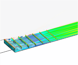
3.3. DNS of supersonic BFS flow
In this section, DNS is performed to reveal the 3-D flow structure and verify the GSA result. The case of h = 7 mm is considered here, which has two stationary and oscillatory modes. Since the most unstable mode at h = 7 mm occurs at the spanwise wavelength of  $\lambda /h = \textrm{1}\textrm{.396}$ (corresponding to β = 4.5), four times the wavelengths are extended in the spanwise directions for the computational region. The distributions of grid cells in the streamwise and wall-normal directions remain unchanged as the adopted medium grid resolution, which is used for computing base flow. Seventy cells are placed uniformly for every spanwise wavelength, resulting in a total of 280 cells in the spanwise direction. The total number of grid cells for DNS is approximately 90 million. The 3-D simulation starts from tu∞/h = 0 to 1510 (i.e. the physical time is 0–20 ms) to obtain a quasi-steady state to resolve the development of three-dimensionality and low-frequency unsteadiness. In the present study, no extra perturbations are imposed in the simulation. It is expected that the growth of instability waves can arise from the exceedingly small perturbations provided by the numerical round-off errors to depict the intrinsic instability predicted by GSA.
To characterize the development of 3-D perturbations with respect to the base flow in terms of the specific spanwise wavelength, the temporal evolution of the spanwise velocity perturbations is extracted for comparison. As illustrated by Cao et al. (Reference Cao, Hao, Klioutchnikov, Olivier and Wen2021b, Reference Cao, Hao, Klioutchnikov, Wen, Olivier and Heufer2022) and Hao et al. (Reference Hao, Cao, Wen and Olivier2021), the averaged spanwise velocity magnitude normalized by the free stream velocity in a streamwise normal plane is calculated using the following equation:
 \begin{equation}{\sigma _w} = \sqrt {\frac{1}{{{N_y}{N_z}}}\sum\limits_{j = 1}^{{N_y}} {\sum\limits_{k = 1}^{{N_z}} {\left( {\frac{w}{{{u_\infty }}}} \right)_{j,k}^2} } } ,\end{equation}
where Ny and Nz are the numbers of grid cells in the wall-normal and spanwise directions, respectively. Figure 14 shows the temporal evolution of the averaged spanwise velocity magnitude in the z–y plane located at x/h = 7.14. This plane is located in the region where the spanwise perturbations are confined; this region represents where the main perturbations occur, as obtained from the GSA result, as shown in figure 10(c). After an initial adjustment owing to the numerical method, the exponential growth rate obtained from DNS shows good agreement with that of the most unstable mode predicted by GSA until tu∞/h = 405, which verifies the fidelity of both GSA and DNS. The initial adjustment could be attributed to slight differences in the numerical methods employed between the 2-D and 3-D simulations. The inherent complexes, additional dimensions and applications of periodic boundary conditions in 3-D simulations can lead to slight discrepancies compared with the flow field extruded from 2-D base flow during the initial transient, which may manifest as the initial adjustment. However, it is well noted that the adjustments can be principally excluded by adapting the numerical method (Hildebrand et al. Reference Hildebrand, Dwivedi, Nichols, Jovanović and Candler2018), but more computational time will be needed to achieve the linear growth stage. After the exponential growth of σw, nonlinear saturation occurs until tu∞/h ≈ 900, and then a quasi-steady state is established. This comparison provides strong evidence that GSA can accurately predict the most unstable mode induced by the global instability of the flow and proves the significant effectiveness of both GSA and DNS.

Figure 14. Temporal evolution of the average absolute spanwise velocity perturbations at x/h = 7.14 obtained from the DNS result compared with the growth rate of the most unstable mode predicted by GSA. Solid line, DNS; dashed line, GSA.
Figure 15(a) shows the contour of the spanwise velocity in the x–y plane of z/h = 0.7143 at tu∞/h = 362.5 in the linear growth stage. The main flow structure is nearly identical to the spanwise velocity perturbations of mode 1L in the case of h = 7 mm predicted by GSA, as shown in figure 10(c), which also confirms that mode 1 dominates the linear growth stage of the 3-D perturbations. Figures 15(b) and 15(c) show the contours of the spanwise velocity at two y–z planes of x/h = 6.8281 and 7.6814, respectively. There is a slight attenuation of the spanwise velocity in the middle of the plane. This phenomenon is likely a result of perturbations that tend to arise from the periodic boundary conditions applied in the spanwise direction. However, this attenuation does not have a significant impact on the growth of the instability wave, as evidenced by figure 14. The perturbations have a periodic distribution with a wavelength of approximately λ/h = 1.3. For a quantitative comparison, the spatial characteristics of the perturbations are provided by the (spatial) power spectral density (PSD) of Cf along the streamline direction, as shown in figure 16. From the PSD of Cf, the peaks at the spanwise wavelength λ/h ≈ 1.3 can be extracted in the region of x ≈ 7, which is more energetic and corresponds well to the region with large spanwise velocity perturbations predicted by GSA. The wavelength λ/h obtained from the PSD is approximately 1.35, which is slightly smaller than the predetermined wavelength λ/h = 1.3916 from the GSA. A closer examination of figure 9 gives an explanation that the growth rates and the structures of mode 1 in the wavelength range of 1.23~1.39 are nearly identical. This observation suggests that the signals detected by DNS may be subject to blurring, resulting in a slight shift in wavelength.

Figure 15. Contours of the spanwise velocity at tu∞/h = 362.5: (a) x–y plane at z/h = 0.7143; (b) y–z plane at x/h = 6.8281, denoted by A in panel (a); and (c) y–z plane at x/h = 7.6814, denoted by B in panel (a).

Figure 16. Power spectral density of the skin friction coefficient on the wall downstream of the step obtained from DNS at tu∞/h = 362.5.
Figure 17 shows the evolution of the spanwise velocities in the later linear stage in an x–y plane of z/h = 0.7143. At tu∞/h = 407.8 and 438.0, the spatial flow structure is still almost identical to that of mode 1 captured by the GSA. The spanwise velocity magnitude increases with time and occupies a larger region. At tu∞/h = 438.0, the perturbations begin to propagate upstream within the primary vortex, resulting in the formation of streak-shaped structures aligned in the streamwise direction. After tu∞/h = 468.2, the streak-shaped structures are strongly distorted and slowly break up into smaller structures. At tu∞/h = 528.7, the flow structure looks like a combination of unstable modes captured by GSA (figures 10 and 11), which hints at the emergence of mode 2 and mode 1S. The non-dimensional frequency of mode 2 from the GSA result is approximately 0.005, which is of the same order as the low frequency (0.009) reported in the large eddy simulation (LES) conducted by Riley, Ranjan & Gaitonde (Reference Riley, Ranjan and Gaitonde2021). Although the Reynolds number and Mach number in the study of Riley et al. (Reference Riley, Ranjan and Gaitonde2021) are higher than those in the present study, it can be speculated that mode 2 can persist in supersonic BFS flow.

Figure 17. Temporal evolution of the spanwise velocities at the x–y plane of z/h = 0.7143 obtained from different times: (a) tu∞/h = 377.6; (b) tu∞/h = 407.8; (c) tu∞/h = 438.0; (d) tu∞/h = 468.2; (e) tu∞/h = 498.5 and (f) tu∞/h = 528.7.
Owing to the existence of global unstable modes, the saturated flow obtained from DNS exhibits a complicated structure in both spatial and temporal space. To further understand the influence of the perturbation on the flow structure, the Cf distributions downstream of the step at different times are shown in figure 18. Isolines of Cf = 0 are used to indicate the separation regions. Note that the vertical solid line at x/h ≈ 3.5 represents the secondary separation line (also see figure 4), which separates the primary–secondary vortices on the wall in the streamwise direction. The second solid line at x/h ≈ 12 is the reattachment line. In the initial stage, the two vertical lines present 2-D characteristics. At the later stage of the linear growth period, the reattachment and secondary separation lines become slightly distorted, but the separation zone retains the original pattern. With increasing time, the reattachment line twists further with a zigzag pattern, and similar features were reported by Cao et al. (Reference Cao, Hao, Klioutchnikov, Olivier and Wen2021b, Reference Cao, Hao, Klioutchnikov, Wen, Olivier and Heufer2022) in their DNS of hypersonic compression corner flows and by Hao et al. (Reference Hao, Fan, Cao and Wen2022) in their DNS of hypersonic double cone flows. Meanwhile, the secondary separation line becomes highly disordered and breaks up into several small separation zones, which are not observed in 2-D simulations. After tu∞/h = 1057.3, the reattachment line presents a harmonic distribution characteristic, exhibiting a wavelength of λ/h ≈ 0.68, which is consistent with the second harmonic of the wavelength of mode 1. Additionally, the line oscillates at a relatively low frequency. Meanwhile, the secondary separation line is fully distorted and cannot be intuitively distinguished. More small bubbles with irregular shapes can be observed and are distributed randomly in the original secondary separation region. The peak of Cf is much higher than that in the linear growth stage, and the streamwise streaky patterns persist downstream of the reattachment line. The streak-like flow structures attest to the phenomena observed by Ginoux (Reference Ginoux1960) and Zhu et al. (Reference Zhu, Yi, Gang and He2015). Thus, it can be concluded from the GSA and DNS results that intrinsic instability is responsible for the generation of streak-like flow structures. Figure 19 shows the power spectral density of the averaged spanwise velocity (σw) at x/h = 7.14 from th/u∞ = 377.6 to 1510.5. Based on the spectrum, the quasi-steady BFS flow exhibits a broadband feature covering the frequency of mode 2. The low-frequency broadband characteristics account for the oscillation of Cf, as shown in figure 18.

Figure 18. Contours of the skin friction coefficient at (a) tu∞/h = 113.3, (b) tu∞/h = 422.9, (c) tu∞/h = 604.2, (d) tu∞/h = 1057.3, (e) tu∞/h = 1283.9 and (f) tu∞/h = 1495.4. Black solid lines, isolines of Cf = 0.

Figure 19. Power spectral density of the averaged spanwise velocity at x/h = 7.14 from tu∞/h = 377.6 to 1510.5.
To closely examine the 3-D flow structures in the separation zone, figure 20 shows the contours of the streamwise velocity u/u∞ (<0.99) on several y–z planes (seven equidistant distributed planes at 6 ≤ x/h ≤ 8) and one x–z plane (at y/h = 0.1) at tu∞/h = 422.9 and tu∞/h = 1283.9, respectively. The isolines of u/u∞ (<0) are superimposed in the equidistantly distributed streamwise planes. The contours of the spanwise velocity are shown on the left. To facilitate processing, the isosurfaces of u = 0 are plotted to characterize the separation zones. At tu∞/h = 422.9, the spanwise perturbations gathered at approximately 6 ≤ x/h ≤ 8 and the primary vortex with a zigzag reattachment line remained smooth. The flow structures are nearly identical to those reconstructed using the global mode and the base flow, as shown in figure 12(a). In the quasi-steady state, the spanwise velocity perturbations propagate upstream and pervade the whole separation zone. The primary vortex is severely corrugated. Several small bubbles form with irregular shapes and are randomly distributed in the secondary vortex, which reinforces the observations based on the skin friction coefficient plotted in figure 18. In addition, streamwise streaks can be observed and do not breakdown downstream. Whether the intrinsic instability is able to trigger a laminar‒turbulent transition at h = 15 mm will be the focus of a future study. That, again, would imply that the streak-like flow structures can be attributed to the intrinsic instability of supersonic BFS flow, which is two-dimensionally stable and destabilized under the influence of 3-D perturbations with a specific spanwise wavelength.

Figure 20. Contours of the streamwise velocity shown on a wall-parallel plane at y/h = 0.1 close to the wall and seven equidistantly distributed streamwise planes superimposed with isolines of streamwise velocity in the range of 0 ≤ x/h ≤ 12 at different times. Contours of the spanwise velocity at the z = 0 plane are shown in panels (c) and (d), respectively. Grey isosurfaces of u = 0 are plotted to represent the separation zones. (a) and (c) tu∞/h = 422.9; (b) and (d) tu∞/h = 1283.9. (The cut-off levels are u/u∞ > 0.99 and u/u∞ > 0 for contours and isolines of streamwise velocity, respectively.)
4. Conclusion
In the present study, DNS and GSA are performed for a supersonic backward-facing step flow where the step heights vary from 5 to 15 mm. The free stream Mach number and Reynolds number based on the flat-plate length are 2.16 and 7.94 × 10⁵, respectively. Owing to the sudden expansion downstream of the step, a large recirculation zone forms, which mainly includes a primary and a secondary zone. More Moffatt vortices can also be observed with sufficient grid resolution near the origin of the step corner. Importantly, the flows for all step heights considered in the present study are stable in a 2-D state; that is, no two-dimensionally unstable mode is found.
GSA shows that the supersonic BFS flow is unstable to 3-D perturbations when the step height h exceeds 5.4 mm in the present study. As the step height approaches 6 mm, a pair of conjugate modes are detected. Then, the pair of conjugate modes merges into two stationary unstable modes at h = 7 mm, and another oscillatory unstable mode is revealed. The spanwise velocity perturbations of the most unstable mode are mainly confined to a small region near the primary vortex core that is located close to the reattachment point, whereas the velocity perturbations in the unstable oscillatory mode almost fill the whole region of the recirculation zone, and are presented as pairs of positive and negative components. Reconstructing the 3-D flow field by superimposing the most unstable mode on the base flow shows that the primary vortex is corrugated and the reattachment line exhibits a zigzag shape. Streamwise vortices occur in the primary vortex, accompanied by the formation of a spanwise array of pairs of positive and negative streamwise perturbations. Furthermore, the energy budget analysis suggests that the instability of supersonic BFS flow is probably of the elliptic type.
A step height of h = 7 mm is selected to conduct a DNS study. The spanwise length of the computational region for DNS is four times the wavelength of the most unstable mode. The exponential linear growth rate obtained from DNS shows good agreement with the predicted rate obtained from GSA, and the most unstable mode (mode 1 predicted by GSA) dominates the linear growth stage, in which the contours of the spanwise velocity coincide with the corresponding spanwise velocity perturbations from GSA. Mode 2 emerges in the later linear growth stage and then affects the flow structure together with mode 1. The saturated flow exhibits a broadband low-frequency unsteadiness characteristic. The boundary-layer streaks and surface friction streaks appear in an oscillatory form with a low frequency. In addition, the separation zone is severely distorted, especially the secondary separation zone that fragments into several small bubbles. No transition is observed in the present case.
In conclusion, the numerical simulations and GSA illustrate that supersonic BFS flow is intrinsically unstable to 3-D perturbations when the step exceeds a certain value. The streak-like flow structures that were observed in supersonic BFS flow can be attributed to the global instability of the separated flow.
Funding
This work is supported by the Hong Kong Research Grants Council (no. 15206519 and no. 25203721), the National Natural Science Foundation of China (no. 12102377 and no. 12332018) and the Hong Kong Scholars Program (no. 2020-043).
Declaration of interests
The authors report no conflict of interest.
Appendix A. Validation of stability analysis
First, the validation of the present global stability analysis code is performed for incompressible lid-driven square cavity flow at Re = 200 based on the side length Ls and the lid velocity uL. Table 2 presents a comparison of the growth rates and frequencies of the least stable eigenmode at different spanwise wavenumbers between the present study and the results from Ramanan & Homsy (Reference Ramanan and Homsy1994) and Theofilis et al. (Reference Theofilis, Duck and Owen2004). The same results are also presented in figure 21 for the variations in the growth rates and frequencies with the spanwise wavenumber. Overall, there is a good quantitative agreement between the present and previous results, indicating the effectiveness of the GSA code used in this study.
Table 2. Comparisons of the frequencies and growth rates of the least stable modes at Re = 200 from β = 1 to 9 with the results of Ramanan & Homsy (Reference Ramanan and Homsy1994) and Theofilis et al. (Reference Theofilis, Duck and Owen2004).


Figure 21. Comparisons of the variations in ωi and ωr with β at Re = 200. Blue dashed line, Theofilis et al. (Reference Theofilis, Duck and Owen2004); green dash-dotted line, Ramanan & Homsy (Reference Ramanan and Homsy1994); red solid line with triangle symbols, the present results.
We also compare our results for compressible open-cavity flow with a length-to-depth ratio of L/D = 2, Ma∞ = 1.4 and Reθ = 56.8 to the results obtained by Sun et al. (Reference Sun, Taira, Cattafesta and Ukeiley2017). Here, the Reynolds number Reθ is based on the initial momentum boundary layer thickness at the cavity leading edge and the free stream values. Table 3 shows the comparisons of the frequencies and growth rates of Rossiter Modes I and II. The obtained frequencies and growth rates are in good agreement with those of Sun et al. (Reference Sun, Taira, Cattafesta and Ukeiley2017).
Table 3. Comparisons of the growth rates and frequencies of Rossiter Mode I and II obtained from Sun et al. (Reference Sun, Taira, Cattafesta and Ukeiley2017) and the present study.

Appendix B. Validation of the numerical simulation code
The PHAROS code used in the present study has been extensively validated with typical benchmark cases in our previous work. The details of the validation cases can be found in these studies. Further validation of the PHAROS code for simulating supersonic BFS flow was performed by comparing it with the experimental results of Smith (Reference Smith1967). The experiment used to validate the PHAROS code was conducted on a BFS model with a step height of 11.252 mm and a flat-plate length of 101.6 mm. The nominal free stream Mach number, total temperature and total pressure are 2.5, 344.44 K and 31026.41 Pa, respectively, resulting in a corresponding Reynolds number based on the flat-plate length of 2.48 × 10⁵. Figure 22 compares the 2-D simulation results from the PHAROS code with the experimental data of Simth (Reference Smith1967) in terms of the wall pressure normalized by the free stream pressure. Note that the experimental results are reproduced from the graph provided by Smith (Reference Smith1967). The wall pressure shows a rise tendency in the reattachment process after the pressure plateau region. In general, the numerical results show good agreement with the experiments in terms of the pressure on the flat plate, the plateau pressure, the pressure rise and the reattachment location. This comparison demonstrates the satisfactory performance of the PHAROS code in simulating supersonic BFS flow.

Figure 22. Comparisons of the wall pressure normalized by the free stream pressure obtained from the 2-D numerical simulations and experiments conducted by Smith (Reference Smith1967).
Appendix C. Determination of critical step height
To determine the onset of linear global instability, the approach described in the previous sections is employed for supersonic BFS flow in the present study by varying the step height from h = 5 mm to 6 mm, with a regular interval of 0.1 mm. The GSA result indicates that the step height at which instability marginally appears is approximately 5.4 mm. At a step height of h = 5.4 mm, the unstable modes are characterized by a pair of oscillatory modes. Figure 23 illustrates the growth rate of modes 1 and 2 as a function of spanwise wavelengths for three critical step heights (i.e. h = 5.3, 5.4 and 5.5 mm). Note that only oscillatory mode 1 is shown in figure 23, since stationary mode 1 concentrates near λ/h ≈ 0.5. At a step height of h = 5.4 mm, the supersonic BFS flow becomes marginally unstable, with the most unstable mode occurring at a spanwise wavelength of λ/h ≈ 3.142. Additionally, a couple of oscillatory unstable modes unstable modes dominate over a very limited range of spanwise wavelength. When the step height is increased to 5.5 mm, mode 2 becomes unstable. Consequently, the distribution of the growth rate, as shown in figure 23, closely resembles the distributions depicted in figure 9(b).

Figure 23. Growth rates of modes 1 and 2 as a function of spanwise wavelengths for different step heights: green, h = 5.3 mm; blue, h = 5.4 mm; red, h = 5.5 mm. (a) Triangle symbols with solid line, oscillatory mode 1; (b) triangle symbols with dash dotted line, oscillatory mode 2.


 Open access