


We have noticed a missing term in the linearisation of the differential contour vector $\boldsymbol{n}_{S}\,\text{d}\unicode[STIX]{x1D6E4}$
, which is a differential of the boundary of a surface
$\boldsymbol{n}_{S}\,\text{d}\unicode[STIX]{x1D6E4}$
, which is a differential of the boundary of a surface $\unicode[STIX]{x1D6F4}$
with normal
$\unicode[STIX]{x1D6F4}$
with normal $\boldsymbol{n}$
perpendicular to
$\boldsymbol{n}$
perpendicular to $\boldsymbol{n}_{S}$
, appearing in some of the expressions given in our recent paper (Rivero-Rodriguez & Scheid Reference Rivero-Rodriguez and Scheid2018). Nevertheless, this term had been considered in the numerical simulations such that the results and conclusions of our paper are not affected. However, this corrigendum aims at clarifying the origin of this term and to provide the correct procedure for the linearisation of
$\boldsymbol{n}_{S}$
, appearing in some of the expressions given in our recent paper (Rivero-Rodriguez & Scheid Reference Rivero-Rodriguez and Scheid2018). Nevertheless, this term had been considered in the numerical simulations such that the results and conclusions of our paper are not affected. However, this corrigendum aims at clarifying the origin of this term and to provide the correct procedure for the linearisation of $\boldsymbol{n}_{S}\,\text{d}\unicode[STIX]{x1D6E4}$
, as well as give the list of the corrected equations with the missing term now included and referenced with the same label as in the original paper preceded by the mark ‘Corrected’. Correct original equations are referenced with their original labels and new equations in this corrigendum are labelled using Roman numbers. First, we proceed to obtain the variation of a differential contour vector by analogy with the variation of a differential surface vector and then we report the modifications that apply to our previous work (Rivero-Rodriguez & Scheid Reference Rivero-Rodriguez and Scheid2018).
$\boldsymbol{n}_{S}\,\text{d}\unicode[STIX]{x1D6E4}$
, as well as give the list of the corrected equations with the missing term now included and referenced with the same label as in the original paper preceded by the mark ‘Corrected’. Correct original equations are referenced with their original labels and new equations in this corrigendum are labelled using Roman numbers. First, we proceed to obtain the variation of a differential contour vector by analogy with the variation of a differential surface vector and then we report the modifications that apply to our previous work (Rivero-Rodriguez & Scheid Reference Rivero-Rodriguez and Scheid2018).
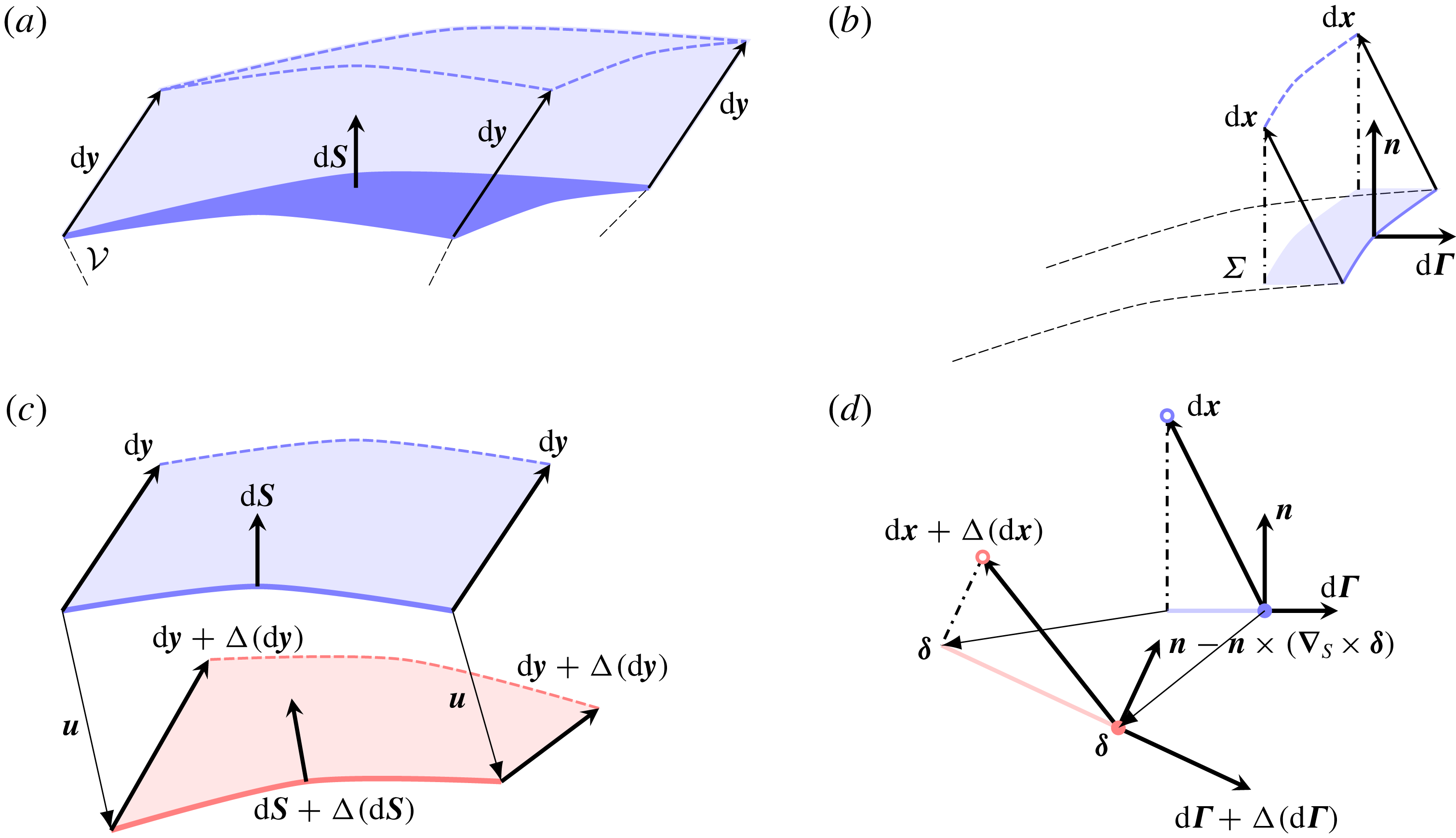
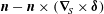
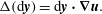
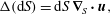
Figure 1. Sketch of (a) a virtual volume $\text{d}\boldsymbol{y}\boldsymbol{\cdot }\text{d}\boldsymbol{S}$
and (b) the projection onto the surface
$\text{d}\boldsymbol{y}\boldsymbol{\cdot }\text{d}\boldsymbol{S}$
and (b) the projection onto the surface $\unicode[STIX]{x1D6F4}$
of a virtual surface
$\unicode[STIX]{x1D6F4}$
of a virtual surface $\text{d}\boldsymbol{x}\boldsymbol{\cdot }\text{d}\unicode[STIX]{x1D71E}$
, as well as their cross-sections before (blue) and after (red) the deformation due to the action (c) of
$\text{d}\boldsymbol{x}\boldsymbol{\cdot }\text{d}\unicode[STIX]{x1D71E}$
, as well as their cross-sections before (blue) and after (red) the deformation due to the action (c) of $\boldsymbol{u}$
and (d) of
$\boldsymbol{u}$
and (d) of $\unicode[STIX]{x1D739}$
, respectively. The surfaces and the contours, respectively represented by
$\unicode[STIX]{x1D739}$
, respectively. The surfaces and the contours, respectively represented by $\text{d}\boldsymbol{S}$
and
$\text{d}\boldsymbol{S}$
and $\text{d}\unicode[STIX]{x1D71E}$
, are depicted in dark colours. The virtual volume
$\text{d}\unicode[STIX]{x1D71E}$
, are depicted in dark colours. The virtual volume $\text{d}\boldsymbol{y}\boldsymbol{\cdot }\text{d}\boldsymbol{S}$
and the projection
$\text{d}\boldsymbol{y}\boldsymbol{\cdot }\text{d}\boldsymbol{S}$
and the projection $\text{d}\boldsymbol{x}\boldsymbol{\cdot }\text{d}\unicode[STIX]{x1D71E}$
on the surface
$\text{d}\boldsymbol{x}\boldsymbol{\cdot }\text{d}\unicode[STIX]{x1D71E}$
on the surface $\unicode[STIX]{x1D6F4}$
of the virtual surface are depicted in light colours. Coloured dashed lines represent the surface and contours after the action of the virtual displacement. Black dash-doted lines represent projection parallel to the normal vectors
$\unicode[STIX]{x1D6F4}$
of the virtual surface are depicted in light colours. Coloured dashed lines represent the surface and contours after the action of the virtual displacement. Black dash-doted lines represent projection parallel to the normal vectors $\boldsymbol{n}$
or
$\boldsymbol{n}$
or $\boldsymbol{n}-\boldsymbol{n}\times (\unicode[STIX]{x1D735}_{\!S}\times \unicode[STIX]{x1D739})$
, accordingly. Black dashed lines represent the volume and surface whose boundary and contour are considered.
$\boldsymbol{n}-\boldsymbol{n}\times (\unicode[STIX]{x1D735}_{\!S}\times \unicode[STIX]{x1D739})$
, accordingly. Black dashed lines represent the volume and surface whose boundary and contour are considered.
The time rate of change of a surface vector was first carried out by Batchelor (Reference Batchelor1967, p. 132). Although the original work is done for time rate of change, we are interested here in the variation of a differential surface vector $\text{d}\boldsymbol{S}$
, defined at the boundary of a volume
$\text{d}\boldsymbol{S}$
, defined at the boundary of a volume ${\mathcal{V}}$
, under the deformation due to any given infinitesimal displacement field
${\mathcal{V}}$
, under the deformation due to any given infinitesimal displacement field $\boldsymbol{u}$
defined on
$\boldsymbol{u}$
defined on ${\mathcal{V}}$
. This derivation is based on the variation of the virtual volume generated by sweeping a differential surface, represented by
${\mathcal{V}}$
. This derivation is based on the variation of the virtual volume generated by sweeping a differential surface, represented by $\text{d}\boldsymbol{S}$
, along the virtual generatrix
$\text{d}\boldsymbol{S}$
, along the virtual generatrix $\text{d}\boldsymbol{y}$
as shown in figure 1(a), which can be written as
$\text{d}\boldsymbol{y}$
as shown in figure 1(a), which can be written as
 $$\begin{eqnarray}\displaystyle \unicode[STIX]{x0394}(\text{d}\boldsymbol{y}\boldsymbol{\cdot }\text{d}\boldsymbol{S})=\unicode[STIX]{x0394}(\text{d}\boldsymbol{y})\boldsymbol{\cdot }\text{d}\boldsymbol{S}+\text{d}\boldsymbol{y}\boldsymbol{\cdot }\unicode[STIX]{x0394}(\text{d}\boldsymbol{S}). & & \displaystyle\end{eqnarray}$$
Following Batchelor (Reference Batchelor1967), the variation of the virtual volume, whose deformation of its cross-section is shown in figure 1(c), writes
 $$\begin{eqnarray}\displaystyle \unicode[STIX]{x0394}(\text{d}\boldsymbol{y}\boldsymbol{\cdot }\text{d}\boldsymbol{S})=\text{d}\boldsymbol{y}\boldsymbol{\cdot }\text{d}\boldsymbol{S}\unicode[STIX]{x1D735}\boldsymbol{\cdot }\boldsymbol{u}, & & \displaystyle\end{eqnarray}$$
and the variation of the virtual generatrix writes
 $$\begin{eqnarray}\displaystyle \unicode[STIX]{x0394}(\text{d}\boldsymbol{y})=\text{d}\boldsymbol{y}\boldsymbol{\cdot }\unicode[STIX]{x1D735}\boldsymbol{u}. & & \displaystyle\end{eqnarray}$$
Since (I) is valid for any virtual generatrix $\text{d}\boldsymbol{y}$
, the variation of
$\text{d}\boldsymbol{y}$
, the variation of $\text{d}\boldsymbol{S}$
then writes, using (II) and (III), as
$\text{d}\boldsymbol{S}$
then writes, using (II) and (III), as
 $$\begin{eqnarray}\displaystyle \unicode[STIX]{x0394}(\text{d}\boldsymbol{S})=\text{d}\boldsymbol{S}\boldsymbol{\cdot }[{\mathcal{I}}\unicode[STIX]{x1D735}\boldsymbol{\cdot }\boldsymbol{u}-(\unicode[STIX]{x1D735}\boldsymbol{u})^{\text{T}}], & & \displaystyle\end{eqnarray}$$
where ${\mathcal{I}}$
is the identity tensor.
${\mathcal{I}}$
is the identity tensor.
Following Stone (Reference Stone1990), after projection of (IV) onto the normal vector $\boldsymbol{n}$
and considering that
$\boldsymbol{n}$
and considering that $\text{d}\boldsymbol{S}=\boldsymbol{n}\,\text{d}S$
, the variation of the differential surface
$\text{d}\boldsymbol{S}=\boldsymbol{n}\,\text{d}S$
, the variation of the differential surface $\text{d}S$
is written as
$\text{d}S$
is written as
 $$\begin{eqnarray}\displaystyle \unicode[STIX]{x0394}(\text{d}S)=\text{d}S\,\unicode[STIX]{x1D735}_{\!S}\boldsymbol{\cdot }\boldsymbol{u}, & & \displaystyle\end{eqnarray}$$
where $\unicode[STIX]{x1D735}_{\!S}={\mathcal{I}}_{S}\boldsymbol{\cdot }\unicode[STIX]{x1D735}$
is the surface gradient operator, and
$\unicode[STIX]{x1D735}_{\!S}={\mathcal{I}}_{S}\boldsymbol{\cdot }\unicode[STIX]{x1D735}$
is the surface gradient operator, and ${\mathcal{I}}_{S}={\mathcal{I}}-\boldsymbol{n}\boldsymbol{n}$
the surface identity tensor.
${\mathcal{I}}_{S}={\mathcal{I}}-\boldsymbol{n}\boldsymbol{n}$
the surface identity tensor.
Analogously to the variation of a differential surface vector, we proceed to obtain the variation of a differential contour vector $\text{d}\unicode[STIX]{x1D71E}=\boldsymbol{n}_{S}\,\text{d}\unicode[STIX]{x1D6E4}$
, defined at the contour of a surface
$\text{d}\unicode[STIX]{x1D71E}=\boldsymbol{n}_{S}\,\text{d}\unicode[STIX]{x1D6E4}$
, defined at the contour of a surface $\unicode[STIX]{x1D6F4}$
with normal
$\unicode[STIX]{x1D6F4}$
with normal $\boldsymbol{n}$
, under the deformation due to any given infinitesimal displacement field
$\boldsymbol{n}$
, under the deformation due to any given infinitesimal displacement field $\unicode[STIX]{x1D739}$
defined on
$\unicode[STIX]{x1D739}$
defined on $\unicode[STIX]{x1D6F4}$
. This derivation is based on the variation of the projection on the surface
$\unicode[STIX]{x1D6F4}$
. This derivation is based on the variation of the projection on the surface $\unicode[STIX]{x1D6F4}$
of the virtual surface generated by sweeping a differential contour, represented by
$\unicode[STIX]{x1D6F4}$
of the virtual surface generated by sweeping a differential contour, represented by $\text{d}\unicode[STIX]{x1D71E}$
, along the virtual generatrix
$\text{d}\unicode[STIX]{x1D71E}$
, along the virtual generatrix $\text{d}\boldsymbol{x}$
as shown in figure 1(b), which can be written as
$\text{d}\boldsymbol{x}$
as shown in figure 1(b), which can be written as
 $$\begin{eqnarray}\displaystyle \unicode[STIX]{x0394}(\text{d}\boldsymbol{x}\boldsymbol{\cdot }\text{d}\unicode[STIX]{x1D71E})=\unicode[STIX]{x0394}(\text{d}\boldsymbol{x})\boldsymbol{\cdot }\text{d}\unicode[STIX]{x1D71E}+\text{d}\boldsymbol{x}\boldsymbol{\cdot }\unicode[STIX]{x0394}(\text{d}\unicode[STIX]{x1D71E}). & & \displaystyle\end{eqnarray}$$
According to (V) and substituting $\text{d}S$
by
$\text{d}S$
by $\text{d}S=\text{d}\boldsymbol{x}\boldsymbol{\cdot }\text{d}\unicode[STIX]{x1D71E}$
and
$\text{d}S=\text{d}\boldsymbol{x}\boldsymbol{\cdot }\text{d}\unicode[STIX]{x1D71E}$
and $\boldsymbol{u}$
by
$\boldsymbol{u}$
by $\unicode[STIX]{x1D739}$
, the variation of the projection on
$\unicode[STIX]{x1D739}$
, the variation of the projection on $\unicode[STIX]{x1D6F4}$
of the virtual surface, whose deformation of its cross-section is shown in figure 1(d), writes
$\unicode[STIX]{x1D6F4}$
of the virtual surface, whose deformation of its cross-section is shown in figure 1(d), writes
 $$\begin{eqnarray}\displaystyle \unicode[STIX]{x0394}(\text{d}\boldsymbol{x}\boldsymbol{\cdot }\text{d}\unicode[STIX]{x1D71E})=\text{d}\boldsymbol{x}\boldsymbol{\cdot }\text{d}\unicode[STIX]{x1D71E}\unicode[STIX]{x1D735}_{S}\boldsymbol{\cdot }\unicode[STIX]{x1D739}, & & \displaystyle\end{eqnarray}$$
and the variation of the virtual generatrix writes
 $$\begin{eqnarray}\displaystyle \unicode[STIX]{x0394}(\text{d}\boldsymbol{x})=\text{d}\boldsymbol{x}\boldsymbol{\cdot }\unicode[STIX]{x1D735}_{\!S}\unicode[STIX]{x1D739}-\text{d}\boldsymbol{x}\boldsymbol{\cdot }\boldsymbol{n}\boldsymbol{n}\times (\unicode[STIX]{x1D735}_{\!S}\times \unicode[STIX]{x1D739}), & & \displaystyle\end{eqnarray}$$
where the first term represents the variation of the components of $\text{d}\boldsymbol{x}$
on the surface, i.e.
$\text{d}\boldsymbol{x}$
on the surface, i.e. $\text{d}\boldsymbol{x}\boldsymbol{\cdot }{\mathcal{I}}_{S}$
, whereas the second term represents the variation of the components of
$\text{d}\boldsymbol{x}\boldsymbol{\cdot }{\mathcal{I}}_{S}$
, whereas the second term represents the variation of the components of $\text{d}\boldsymbol{x}$
out of the surface, i.e.
$\text{d}\boldsymbol{x}$
out of the surface, i.e. $\text{d}\boldsymbol{x}\boldsymbol{\cdot }\boldsymbol{n}\boldsymbol{n}$
, due to the rotation of the surface by an angle
$\text{d}\boldsymbol{x}\boldsymbol{\cdot }\boldsymbol{n}\boldsymbol{n}$
, due to the rotation of the surface by an angle $\unicode[STIX]{x1D735}_{\!S}\times \unicode[STIX]{x1D739}$
. It is worth noting that the latter contribution is the one originally missing and has not its analogue in the similar case of
$\unicode[STIX]{x1D735}_{\!S}\times \unicode[STIX]{x1D739}$
. It is worth noting that the latter contribution is the one originally missing and has not its analogue in the similar case of $\unicode[STIX]{x0394}(\text{d}\boldsymbol{y})$
, because
$\unicode[STIX]{x0394}(\text{d}\boldsymbol{y})$
, because $\text{d}\boldsymbol{y}$
is not only defined in a surface but in a volume.
$\text{d}\boldsymbol{y}$
is not only defined in a surface but in a volume.
Since (D 2) is valid for any virtual generatrix $\text{d}\boldsymbol{x}$
, the variation of
$\text{d}\boldsymbol{x}$
, the variation of $\text{d}\unicode[STIX]{x1D71E}$
then writes, using (VI) and (VII), as
$\text{d}\unicode[STIX]{x1D71E}$
then writes, using (VI) and (VII), as
 $$\begin{eqnarray}\displaystyle \unicode[STIX]{x0394}(\text{d}\unicode[STIX]{x1D71E})=\text{d}\unicode[STIX]{x1D71E}\boldsymbol{\cdot }[{\mathcal{I}}_{S}\unicode[STIX]{x1D735}_{\!S}\boldsymbol{\cdot }\unicode[STIX]{x1D739}-(\unicode[STIX]{x1D735}_{\!S}\unicode[STIX]{x1D739})^{\text{T}}+\boldsymbol{n}\times (\unicode[STIX]{x1D735}_{\!S}\times \unicode[STIX]{x1D739})\boldsymbol{n}]. & & \displaystyle\end{eqnarray}$$
In the original paper (Rivero-Rodriguez & Scheid Reference Rivero-Rodriguez and Scheid2018), the displacement is considered normal to the surface, i.e. $\unicode[STIX]{x1D739}=\unicode[STIX]{x1D6FF}\boldsymbol{n}$
, which substituted in (VIII) leads, using
$\unicode[STIX]{x1D739}=\unicode[STIX]{x1D6FF}\boldsymbol{n}$
, which substituted in (VIII) leads, using $\unicode[STIX]{x1D735}_{\!S}\times \boldsymbol{n}=\mathbf{0}$
and double vector products properties, to
$\unicode[STIX]{x1D735}_{\!S}\times \boldsymbol{n}=\mathbf{0}$
and double vector products properties, to
 $$\begin{eqnarray}\displaystyle \unicode[STIX]{x0394}(\text{d}\unicode[STIX]{x1D71E})=\text{d}\unicode[STIX]{x1D71E}\boldsymbol{\cdot }[{\mathcal{I}}_{S}\unicode[STIX]{x1D6FF}\unicode[STIX]{x1D735}_{\!S}\boldsymbol{\cdot }\boldsymbol{n}-(\unicode[STIX]{x1D735}_{\!S}\boldsymbol{n}\unicode[STIX]{x1D6FF})^{\text{T}}+(\unicode[STIX]{x1D735}_{\!S}\unicode[STIX]{x1D6FF})\boldsymbol{n}]. & & \displaystyle\end{eqnarray}$$
Despite this additional term, the results obtained from the numerical simulations are not affected. It is because for the perturbation of the surface tension in the numerical method, analogous to that of (D 1) using $\unicode[STIX]{x1D711}=Ca^{-1}$
, we had used the right-hand side of the original (D 5), which is correct. Only, the left-hand side should be corrected as follows
$\unicode[STIX]{x1D711}=Ca^{-1}$
, we had used the right-hand side of the original (D 5), which is correct. Only, the left-hand side should be corrected as follows
 $$\begin{eqnarray}\displaystyle \boldsymbol{n}_{S}\boldsymbol{\cdot }[\unicode[STIX]{x1D717}{\mathcal{I}}_{S}-(\unicode[STIX]{x1D735}_{\!S}\unicode[STIX]{x1D6FF}\boldsymbol{n})^{\text{T}}+(\unicode[STIX]{x1D735}_{\!S}\unicode[STIX]{x1D6FF})\boldsymbol{n}]=\boldsymbol{n}_{S}\boldsymbol{\cdot }(\unicode[STIX]{x1D717}{\mathcal{I}}_{S}-\unicode[STIX]{x1D6FF}\unicode[STIX]{x1D735}_{\!S}\boldsymbol{n})-\boldsymbol{n}_{S}\times [\unicode[STIX]{x1D735}_{\!S}\times (\unicode[STIX]{x1D6FF}\boldsymbol{n})], & & \displaystyle \nonumber\\ \displaystyle & & \displaystyle\end{eqnarray}$$
where $\unicode[STIX]{x1D717}=\unicode[STIX]{x1D735}_{\!S}\boldsymbol{\cdot }\unicode[STIX]{x1D739}$
, the symmetry of the curvature tensor implying that
$\unicode[STIX]{x1D717}=\unicode[STIX]{x1D735}_{\!S}\boldsymbol{\cdot }\unicode[STIX]{x1D739}$
, the symmetry of the curvature tensor implying that $\unicode[STIX]{x1D735}_{\!S}\boldsymbol{n}=(\unicode[STIX]{x1D735}_{\!S}\boldsymbol{n})^{\text{T}}$
, and
$\unicode[STIX]{x1D735}_{\!S}\boldsymbol{n}=(\unicode[STIX]{x1D735}_{\!S}\boldsymbol{n})^{\text{T}}$
, and $\boldsymbol{n}\boldsymbol{\cdot }\boldsymbol{n}_{S}=0$
have been used. Numerical computations of the equality (Corrected D 5) confirm its correctness.
$\boldsymbol{n}\boldsymbol{\cdot }\boldsymbol{n}_{S}=0$
have been used. Numerical computations of the equality (Corrected D 5) confirm its correctness.
In order to properly add this additional term where necessary in the original manuscript we provide the modified equations, ordered by appearance in the original paper,
 $$\begin{eqnarray}\boldsymbol{n}\boldsymbol{\cdot }\unicode[STIX]{x27E6}\unicode[STIX]{x1D749}_{0}\unicode[STIX]{x27E7}-\boldsymbol{D}_{\!S}\boldsymbol{\cdot }(\unicode[STIX]{x1D6FF}_{1}\unicode[STIX]{x27E6}\unicode[STIX]{x1D749}_{-1}\unicode[STIX]{x27E7})=\boldsymbol{D}_{\!S}\boldsymbol{\cdot }[\unicode[STIX]{x1D717}_{1}{\mathcal{I}}_{S}-(\unicode[STIX]{x1D735}_{\!S}\unicode[STIX]{x1D6FF}_{1}\boldsymbol{n})^{\text{T}}+(\unicode[STIX]{x1D735}_{\!S}\unicode[STIX]{x1D6FF}_{1})\boldsymbol{n}]\quad \text{at }\unicode[STIX]{x1D6F4}_{B_{0}},\end{eqnarray}$$
 $$\begin{eqnarray}\boldsymbol{n}\boldsymbol{\cdot }\unicode[STIX]{x27E6}\unicode[STIX]{x1D749}_{1}\unicode[STIX]{x27E7}-\boldsymbol{D}_{\!S}\boldsymbol{\cdot }(\unicode[STIX]{x1D6FF}_{2}\unicode[STIX]{x27E6}\unicode[STIX]{x1D749}_{-1}\unicode[STIX]{x27E7}+\unicode[STIX]{x1D6FF}_{1}\unicode[STIX]{x27E6}\unicode[STIX]{x1D749}_{0}\unicode[STIX]{x27E7})-\unicode[STIX]{x1D6FF}_{1}\,\boldsymbol{f}_{0}=\boldsymbol{D}_{\!S}\boldsymbol{\cdot }[\unicode[STIX]{x1D717}_{2}{\mathcal{I}}_{S}-(\unicode[STIX]{x1D735}_{\!S}\unicode[STIX]{x1D6FF}_{2}\boldsymbol{n})^{\text{T}}+(\unicode[STIX]{x1D735}_{\!S}\unicode[STIX]{x1D6FF}_{2})\boldsymbol{n}]\quad \text{at }\unicode[STIX]{x1D6F4}_{B_{0}},\end{eqnarray}$$
 $$\begin{eqnarray}\boldsymbol{n}\times \boldsymbol{D}_{\!S}\boldsymbol{\cdot }[\unicode[STIX]{x1D6FF}_{1}\unicode[STIX]{x27E6}\unicode[STIX]{x1D749}_{-1}\unicode[STIX]{x27E7}+\unicode[STIX]{x1D717}_{1}{\mathcal{I}}_{S}-(\unicode[STIX]{x1D735}_{\!S}\unicode[STIX]{x1D6FF}_{1}\boldsymbol{n})^{\text{T}}+(\unicode[STIX]{x1D735}_{\!S}\unicode[STIX]{x1D6FF}_{1})\boldsymbol{n}]=\mathbf{0},\end{eqnarray}$$
 $$\begin{eqnarray}-\boldsymbol{n}\hat{p}_{s0}=\boldsymbol{D}_{\!S}\boldsymbol{\cdot }[\unicode[STIX]{x1D6FF}_{1}\unicode[STIX]{x27E6}\unicode[STIX]{x1D749}_{-1}\unicode[STIX]{x27E7}+\unicode[STIX]{x1D717}_{1}{\mathcal{I}}_{S}-(\unicode[STIX]{x1D735}_{\!S}\unicode[STIX]{x1D6FF}_{1}\boldsymbol{n})^{\text{T}}+(\unicode[STIX]{x1D735}_{\!S}\unicode[STIX]{x1D6FF}_{1})\boldsymbol{n}],\end{eqnarray}$$
 $$\begin{eqnarray}\int _{\unicode[STIX]{x1D6F4}}\boldsymbol{D}_{\!S}\unicode[STIX]{x1D711}\,\text{d}\unicode[STIX]{x1D6F4}=\int _{\unicode[STIX]{x1D6F4}_{0}}\boldsymbol{D}_{\!S}\boldsymbol{\cdot }\{[(1+\unicode[STIX]{x1D717}){\mathcal{I}}-(\unicode[STIX]{x1D735}_{\!S}\unicode[STIX]{x1D6FF}\boldsymbol{n})^{\text{T}}+(\unicode[STIX]{x1D735}_{\!S}\unicode[STIX]{x1D6FF})\boldsymbol{n}]\unicode[STIX]{x1D711}\}\,\text{d}\unicode[STIX]{x1D6F4}.\end{eqnarray}$$
We would like to emphasise that the missing rotation contribution of the surface perturbation in the equations corrected above has been properly accounted for in the numerical procedure such that the original results are still valid.
Beside the modifications it introduces in our previous paper (Rivero-Rodriguez & Scheid Reference Rivero-Rodriguez and Scheid2018), we believe this procedure could be of interest for other purposes involving surface differential calculus.

