


1. Introduction
Most flows in nature and engineering are bounded by solid walls. In general, the flow in the immediate vicinity – at a molecular scale distance – of the wall has the velocity of the wall, the so-called no-slip boundary condition. As a consequence, a steep gradient in the mean streamwise velocity profiles exists within the boundary layer (BL) region between the wall and the freely flowing fluid above. In the BL, the action of viscosity against the gradient of the streamwise velocity results in viscous dissipation, the conversion of kinetic energy into heat.
1.1. Turbulent flow over a flat plate: Prandtl–von Kárman BL theory
For slowly flowing fluids (low Reynolds numbers), the edge of the BL remains smooth, and the fluid flow in the BL is two-dimensional. This laminar BL is described by the famous Prandtl–Blasius self-similar solution (Schlichting Reference Schlichting1979). However, for fast flowing fluids (high Reynolds numbers), the BL becomes turbulent, and the flow inside the BL becomes vortical and three-dimensional. Although exact solutions of these turbulent BLs do not exist, a well-established functional form of the mean streamwise velocity can be obtained based on simple dimensional arguments (Schlichting Reference Schlichting1979). The hallmark result therefrom can be obtained by realizing that the mean streamwise velocity gradient in the wall-normal direction ( ${\textrm {d}u}/{\textrm {d}y}$) is a function of two dimensionless parameters only (Pope Reference Pope2000),
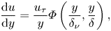 \begin{equation} \frac{\textrm{d}u}{\textrm{d}y} = \frac{u_{\tau}}{y}\varPhi \left( \frac{y}{\delta_{\nu}},\frac{y}{\delta} \right), \end{equation}
where  $u_{\tau }$ is the friction velocity defined as $u_{\tau }=\sqrt [\cdot ]{\tau _w/\rho }$, $\tau _w$ is the mean wall shear stress, $\rho$ is the fluid density, $\delta$ is the outer length scale (e.g. the BL thickness) and $\delta _{\nu }$ is the viscous length scale $\delta _{\nu }=\nu /u_{\tau }$, with $\nu$ the kinematic viscosity of the fluid. Non-dimensionalization by the viscous scales $u_{\tau }$ and $\delta _{\nu }$ is indicated by a superscript ‘+’. The friction Reynolds number based on these viscous quantities is $Re_{\tau } = {u_{\tau }\delta }/{\nu }={\delta }/{\delta _{\nu }}$, and $u_{\tau }=u_{\tau ,i}$, where the subscript $i$ refers to the inner cylinder. For Taylor–Couette (TC) turbulence $\delta =d/2$, with $d$ the gap width between the two rotating cylinders. If we assume that the dependence of the gradient of the mean velocity on viscosity vanishes with increasing $Re_{\tau }$, the yet undefined function $\varPhi ({y}/{\delta _{\nu }},{y}/{\delta })$ must go to a constant ( $=\kappa ^{-1}$) when $\delta _{\nu } \ll y \ll \delta$, which is known as the inertial sublayer. In this limit, we can integrate (1.1) and arrive at the celebrated logarithmic law of the wall for turbulent BLs over a flat surface
 \begin{equation} u^{+} = \kappa^{-1} \log{y^{+}} + B. \end{equation}
This law is connected with the names of Prandtl and von Kármán. It is supported by overwhelming experimental and numerical evidence (e.g. Smits, McKeon & Marusic Reference Smits, McKeon and Marusic2011). The values of the two parameters are  $\kappa \approx 0.39$ and $B\approx 5.0$.
An important extension of the theory concerns buoyancy stratified BLs, where an additional forcing acts on the wall-normal momentum component. A prominent example of such a system is the atmospheric surface layer, where thermal forcing stabilizes or destabilizes the flow. The thermal stratification introduces, aside from  $\delta _{\nu }$ and $\delta$, a third relevant length scale: the Obukhov length $L_{ob}$ (introduced in the year 1946 cf. Obukhov Reference Obukhov1971). This length $L_{ob}$ is proportional to the distance from the wall above which the production of turbulence is significantly affected by buoyancy, and below which the production of turbulence is governed purely by shear. With the introduction of this length $L_{ob}$, (1.1) becomes
 \begin{equation} \frac{\textrm{d}u}{\textrm{d}y} = \frac{u_{\tau}}{y}\varPhi \left(\frac{y}{\delta_{\nu}},\frac{y}{\delta}, \frac{y}{L_{ob}} \right), \end{equation}
which was first proposed by Monin & Obukhov (Reference Monin and Obukhov1954). For the inertial sublayer viscous effects and the domain size effects are negligible ( $\delta _{\nu } \ll y \ll \delta$) and only the dependence on ${y}/{L_{ob}}$ remains. Various empirical fits exist for $\varPhi ({y}/{L_{ob}})$. Evidently, in the limit of ${y}/{L_{ob}}\ll 1$ they must obey $\varPhi ({y}/{L_{ob}})=\kappa ^{-1}$, thus indicating that buoyancy plays no role. We point to § 4 of Monin & Yaglom (Reference Monin and Yaglom1975) for an in-depth analysis of stratified BLs.
1.2. Turbulent flow with streamwise curvature: Taylor–Couette turbulence
Whereas flat plate BLs are often studied, and the existence of a logarithmic profile of the mean streamwise velocity is well established, the study of flows with streamwise curvature is less developed, despite its ubiquity, e.g. ship hulls or turbomachinery. In this paper, we attempt to narrow this gap. One canonical system for flow in a curved geometry is TC flow. TC flow is the shear-driven flow in between two coaxial, independently rotating cylinders. Since the physical system is closed, one can derive a global balance between the differential rotation of the cylinders and the total energy dissipation in the flow, which is directly related to the torque ( $T$) on any of the cylinders (Grossmann, Lohse & Sun Reference Grossmann, Lohse and Sun2016).
The dimensionless torque  $G$ is defined as $G\equiv T/(\rho \nu ^{2}L_z)$, where $L_z$ is the height of the cylinder. It depends on the Reynolds numbers of the inner and outer cylinder, defined as $Re_{i,o}=\omega _{i,o}r_{i,o}d/\nu$. Here, $r_{i,o}$ is the radius of the inner (outer) cylinder and $\omega _{i,o}$ is the angular velocity of the inner (outer) cylinder. The relation $G(Re_i, Re_o, \eta )$ is directly connected to the structure of the mean velocity profile. Uncovering this relation – for its fundamental implications and practical relevance – can be considered the primary research question.
In this paper we consider pure inner cylinder rotation (i.e. outer cylinder Reynolds number is zero  $Re_o=0$), for which, in the laminar case, Taylor (Reference Taylor1923) derived that $G\propto Re$. For intermediate $Re$, Marcus (Reference Marcus1984) – in analogy to the work of Malkus & Veronis (Reference Malkus and Veronis1958) on Rayleigh–Bénard (RB) flow – argued by exploring marginal stability arguments that $G\propto Re^{5/3}$. He modelled the flow domain as being partitioned into a turbulent bulk region with constant angular momentum $L$ (Townsend Reference Townsend1956) and two laminar BLs. For high but finite $Re$, the BLs become turbulent (Grossmann & Lohse Reference Grossmann and Lohse2012; Ostilla-Mónico et al. Reference Ostilla-Mónico, Verzicco, Grossmann and Lohse2015a; Krug et al. Reference Krug, Yang, de Silva, Ostilla-Mónico, Verzicco, Marusic and Lohse2017), and the effective scaling exponent increases with increasing $Re$ (Lathrop, Fineberg & Swinney Reference Lathrop, Fineberg and Swinney1992a,Reference Lathrop, Fineberg and Swinneyb). Analogous to the interpretation of the strongly turbulent regime by Kraichnan (Reference Kraichnan1962) and Chavanne et al. (Reference Chavanne, Chilla, Castaing, Hebral, Chabaud and Chaussy1997) in RB flow, Grossmann & Lohse (Reference Grossmann and Lohse2011) derived logarithmic corrections to the $G(Re)$ scaling, coming from the turbulent BLs, such that $G\propto Re^{2} \times \log (Re)\text {-corrections}$. Recently, Cheng, Pullin & Samtaney (Reference Cheng, Pullin and Samtaney2020) obtained an accurate calculation of the torque by matching the BL and bulk velocity profiles (here referred to as the CPS model).
High-fidelity data on the structure of the BL are essential for testing all proposed scaling relationships. Therefore, much work has been carried out to determine the mean streamwise velocity profile at high  $Re$. Huisman et al. (Reference Huisman, Scharnowski, Cierpka, Kähler, Lohse and Sun2013) used particle image velocimetry (PIV) and laser doppler velocimetry to study the turbulent BL at an unprecedented resolution. For $\eta =0.716$, where $\eta$ is the radius ratio, they find that for high $Re_i$, i.e. $Re_i=O(10^{6})$, the classical logarithmic BL exists only in a very limited spatial region of $50 < y^{+} < 600$. van der Veen et al. (Reference van der Veen, Huisman, Merbold, Harlander, Egbers, Lohse and Sun2016) employed PIV to study the velocity profiles at low radius ratio of $\eta =0.50$, for which the curvature effects are stronger, and find no von Kármán type logarithmic BL. For $\eta =0.91$, Ostilla-Mónico et al. (Reference Ostilla-Mónico, van der Poel, Verzicco, Grossmann and Lohse2014a) and Ostilla-Mónico et al. (Reference Ostilla-Mónico, Verzicco, Grossmann and Lohse2015a) employed direct numerical simulations (DNSs) and find that the slope of the mean streamwise velocity profile is ever changing with $Re_i$, at least up to $Re_i=O(10^{5})$. We further note that Grossmann, Lohse & Sun (Reference Grossmann, Lohse and Sun2014) argue that the appropriate velocity that obeys the classical von Kármán profile is the angular velocity, rather than the streamwise velocity, based on conservation laws of the Navier–Stokes equations in this axial symmetry.
In this paper we will explain that the introduction of a curvature length scale delineates the region where one can expect a shear-dominated turbulent BL and another region where curvature effects will alter the structure of the flow, similar as the Obukhov length in stratified shear flow separates the shear-dominated regime from the buoyancy-dominated regime. This paper is organized as follows: in § 2 we will give the Navier–Stokes equations and boundary conditions for TC flow. In § 3 we will discuss the used datasets. We will then, in § 4, derive a functional form for the angular velocity throughout the entire BL for arbitrary Reynolds numbers but only for pure inner cylinder (IC) rotation. We extend the theory towards varying radius ratios in § 5. Finally, we match the BL and bulk velocity profiles and arrive at a new functional form for  $Nu(Ta)$ and ${C}_{f}({Re}_i)$ for TC in § 6. The paper ends with conclusions and an outlook.
2. Navier–Stokes equations for Taylor–Couette flow
When the inner cylinder rotates and the outer cylinder (OC) remains stationary (the case to which we restrict ourselves in this paper), TC flow is linearly unstable (Rayleigh Reference Rayleigh1916). The ratio between the destabilizing centrifugal force and the stabilizing viscous force is expressed by the Taylor number (Taylor Reference Taylor1923),
 \begin{equation} Ta = \frac{(1+\eta)^{4}}{64\eta^{2}}\frac{(r_o-r_i)^{2}(r_i+r_o)^{2}(\omega_i-\omega_o)^{2}}{\nu^{2}}. \end{equation}
The Reynolds number  $Re_{i,o}$ is related to $Ta$ via the relation $Re_i-\eta Re_o={Ta^{1/2}}/{f(\eta )}$ with $f(\eta ) = {(1+\eta )^{3}}/{8\eta ^{2}}$. Eckhardt, Grossmann & Lohse (Reference Eckhardt, Grossmann and Lohse2007) showed that the mean angular velocity flux
 \begin{equation} J^{\omega} = r^{3} \large[\langle u_r \omega \rangle_{A(r),t} - \nu \partial_r \langle \omega \rangle_{A(r),t}\large] \end{equation}
is independent of  $r$, where $\langle \cdot \rangle _{A(r),t}$ refers to averaging over a cylindrical surface $A(r)$ and time $t$. The torque $T$ per unit length is related to $J^{\omega }$ by $T = 2{\rm \pi} \rho J^{\omega }$. Therefore also $T$ is constant with $r$.
$r$.
TC flow, see the schematic in figure 1, is described by the three components of the Navier–Stokes equations in an inertial frame in cylindrical coordinates, as in Landau & Lifshitz (Reference Landau and Lifshitz1987), with  $w_r$ the radial velocity, $u_{\theta }$ the azimuthal velocity and $v_z$ the axial velocity
 \begin{gather} \partial_t w_r + (\boldsymbol{u}\boldsymbol{\cdot} \boldsymbol{\nabla})w_r -\frac{u_{\theta}^{2}}{r} = -\partial_r P_t + \nu \left \{\mathcal{4} w_r - \frac{2}{r^{2}}\partial_{\theta} u_{\theta} - \frac{w_r}{r^{2}} \right \}, \end{gather}
 \begin{gather} \partial_t u_{\theta} + (\boldsymbol{u}\boldsymbol{\cdot} \boldsymbol{\nabla})u_{\theta} + \frac{w_r u_{\theta}}{r} = -\frac{1}{r}\partial_{\theta} P_t + \nu \left \{\mathcal{4} u_{\theta} + \frac{2}{r^{2}}\partial_{\theta} w_r - \frac{u_{\theta}}{r^{2}} \right \}, \end{gather}
 \begin{gather} \partial_tv_z + (\boldsymbol{u}\boldsymbol{\cdot} \boldsymbol{\nabla})v_z = -\partial_z P_t + \nu \mathcal{4} v_z, \end{gather}
where the operators are
 \begin{equation} (\boldsymbol{u}\boldsymbol{\cdot} \boldsymbol{\nabla})f = w_r\partial_r f + \frac{u_{\theta}}{r}\partial_{\theta} f + v_z\partial_z f, \end{equation}
and
 \begin{equation} \mathcal{4}f = \frac{1}{r}\partial_r (r\partial_r f) + \frac{1}{r^{2}}\partial_{\theta}^{2} f + \partial_z^{2} f, \end{equation}
with for IC rotation only, the boundary conditions  $w_r(r_i)=w_r(r_o)=0$, $v_z(r_i)=v_z(r_o)=0$, $u_{\theta }(r_i)=r_i\omega _i$ and $u_{\theta }(r_o)=r_o\omega _o=0$. Note that $P_t$ is the kinematic pressure, and $\rho P_t$ is the physical pressure. The continuity equation reads
 \begin{equation} \frac{1}{r}\partial_r(rw_r) + \frac{1}{r}\partial_{\theta} u_{\theta} + \partial_z v_z =0. \end{equation}
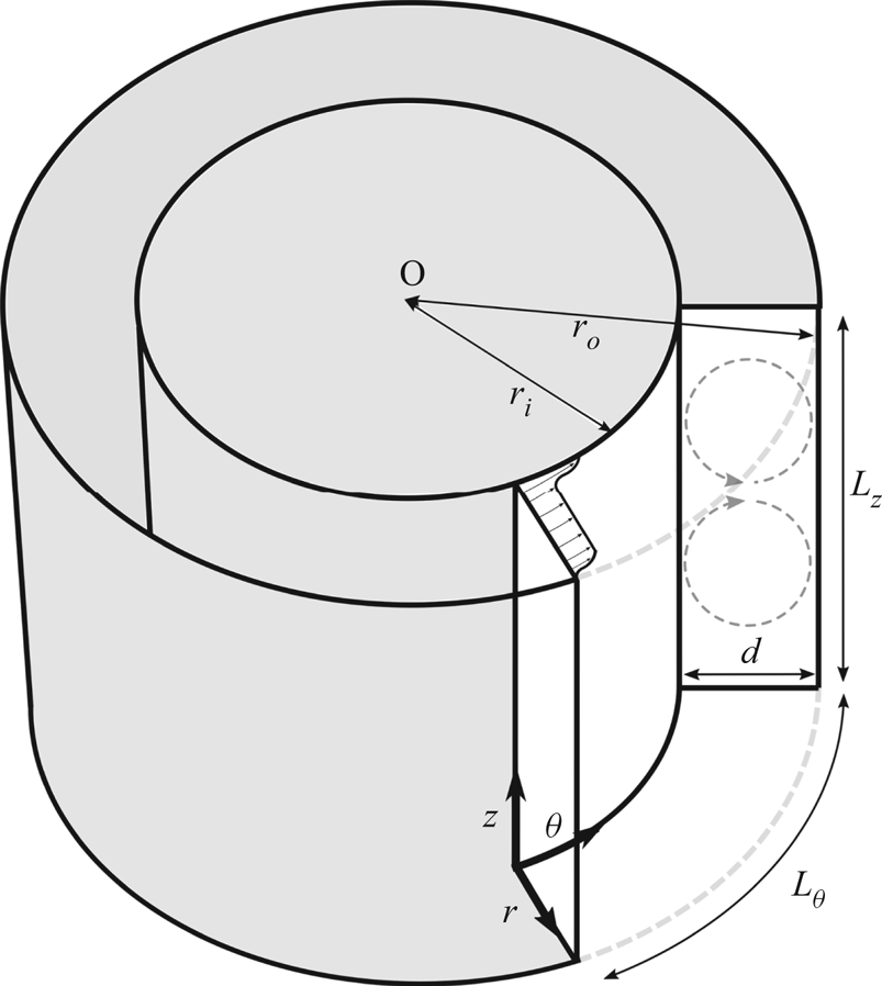
Figure 1. Schematic of TC flow including the coordinate directions  $(\theta , z, r)$, IC radius $r_i$, OC radius $r_o$, gap width $d$, the spanwise (axial) extent of the flow domain $L_z$ and the streamwise extent of the flow domain $L_{\theta }$, which is used in DNSs that employ periodic boundary conditions in the azimuthal directions. $\eta =r_i/r_o$ is the radius ratio. The grey dashed circular arrows represent the turbulent Taylor vortices.
3. Employed datasets
In this paper we apply our analysis to published datasets with varying radius ratio, see table 1 in the appendix. We now briefly describe the techniques that are used to acquire these datasets. However, we refer to the original papers for more details.
Table 1. Used datasets. The curvature Obukhov length  $L_{c}^{+}$ and friction Reynolds number $Re_{\tau }$ at varying $Ta$,
$Ta$,  $Re_i$ and radius ratio $\eta$.
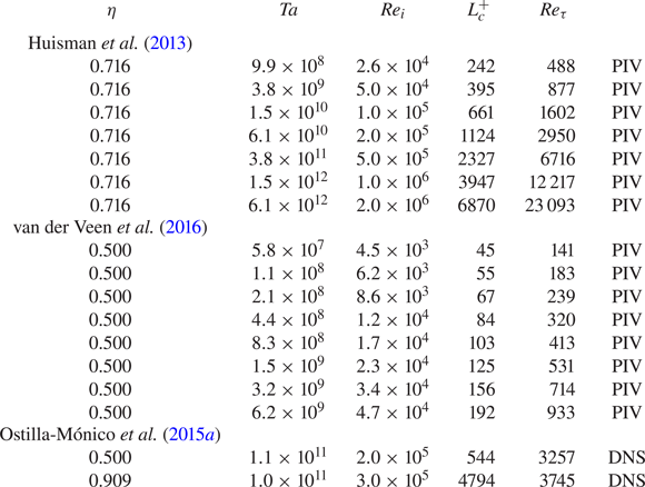
Huisman et al. (Reference Huisman, Scharnowski, Cierpka, Kähler, Lohse and Sun2013) did experiments on highly turbulent inner cylinder rotating TC flow with the Twente turbulent TC facility ( $T^{3}C$) (van Gils et al. Reference van Gils, Bruggert, Lathrop, Sun and Lohse2011a), with the radius ratio $\eta =0.716$ and the aspect ratio $\varGamma =11.7$. In particular, they carried out PIV and particle tracking velocimetry to measure the mean and the variance of the streamwise velocity profiles at $9.9\times 10^{8} \le Ta \le 6.2\times 10^{12}$, for both the IC BL and the OC BL.
van der Veen et al. (Reference van der Veen, Huisman, Merbold, Harlander, Egbers, Lohse and Sun2016) performed experiments on turbulent TC flow in the classical turbulent regime (i.e. before the BLs become turbulent) with the Cottbus TC facility (Merbold, Brauckmann & Egbers Reference Merbold, Brauckmann and Egbers2013), with radius ratio  $\eta =0.50$ and aspect ratio $\varGamma =20$. They carried out PIV to measure the mean streamwise and wall-normal velocity profiles at $5.8\times 10^{7} \le Ta \le 6.2\times 10^{9}$. Although van der Veen et al. (Reference van der Veen, Huisman, Merbold, Harlander, Egbers, Lohse and Sun2016) carried out both counter rotation and pure IC rotation experiments, we will discuss here the latter dataset only.
Ostilla-Mónico et al. (Reference Ostilla-Mónico, Verzicco, Grossmann and Lohse2015a) carried out DNSs of highly turbulent IC rotating TC flow by using a second-order finite-difference scheme (Verzicco & Orlandi Reference Verzicco and Orlandi1996; van der Poel et al. Reference van der Poel, Ostilla-Mónico, Donners and Verzicco2015). With a radius ratio of  $\eta =0.909$ they simulated three cases with $1.1\times 10^{10} \le Ta \le 1.0\times 10^{11}$. Additionally, they simulated a large gap case, $\eta =0.5$, with $Ta=1.1\times 10^{11}$. For all cases the aspect ratio was fixed at $\varGamma =2{\rm \pi} /3$. We refer to Ostilla-Mónico, Verzicco & Lohse (Reference Ostilla-Mónico, Verzicco and Lohse2015b) who found that the aspect ratios of the numerical simulations are sufficiently large to obtain the correct velocity profiles.
4. Velocity profiles in Taylor–Couette turbulence
Whereas the effects of spanwise curvature on the velocity profiles in pipe flow have been investigated before (Grossmann & Lohse Reference Grossmann and Lohse2017), in this section we set out to develop a new functional form of the mean angular velocity profile  $\omega ^{+}(y^{+})$ (with $\omega ^{+} = \omega /\omega _{\tau }$, $\omega _{\tau ,(i,o)}=u_{\tau ,(i,o)}/r_{(i,o)}$, $\omega = \omega _i - u_{\theta }/r$ for the IC BL and $\omega =u_{\theta }/r$ for the OC BL) in that part of the IC BL and OC BL where the streamwise curvature effects are significant. Note that (1.1) can also be postulated for $\omega (y)$, so that the gradient becomes
 \begin{equation} \frac{\textrm{d}\omega}{\textrm{d}y} = \frac{\omega_{\tau}}{y}\varPhi_{\omega} \left( \frac{y}{\delta_{\nu}},\frac{y}{\delta} \right), \end{equation}
where  $\varPhi _{\omega } ({y}/{\delta _{\nu }},{y}/{\delta } )$ goes to a constant in the inertial region $\delta _{\nu } \ll y \ll \delta$. We follow the conclusion of Grossmann et al. (Reference Grossmann, Lohse and Sun2014), namely that near the wall the angular velocity $\omega ^{+}(y^{+})$ fits to a logarithmic form closer than the azimuthal velocity $u^{+}(y^{+})$, and we apply our analysis to $\omega ^{+}(y^{+})$. For reference we have added figure 12 in the appendix, where we apply the analysis (see following pages) to the azimuthal velocity profile.
In § 4.1 we first derive the curvature Obukhov length and then apply our analysis to the highest  $Re$ dataset available (Huisman et al. Reference Huisman, Scharnowski, Cierpka, Kähler, Lohse and Sun2013). Subsequently, we analyse both the IC BL (§ 4.2) and OC BL (§ 4.4) and in § 4.3 also the constant angular momentum region in the bulk.
4.1. Derivation of the curvature Obukhov length  $L_c$
$L_c$

Following Bradshaw (Reference Bradshaw1969), we draw the analogy between the effects of buoyancy and streamline curvature on turbulent shear flow. Therefore it is informative to assess the balance of turbulent kinetic energy (TKE) in the flow. To do so, we first Reynolds decompose the velocity and pressure fields ((2.3)–(2.5)), such that  $\boldsymbol {v} = \boldsymbol {U} + \boldsymbol {u}$, where $\boldsymbol {v}=(w_r, u_{\theta }, v_z)$ is the full velocity, $\boldsymbol {U}=(W,U,V)$ is the time averaged velocity and $\boldsymbol {u}= (w,u,v)$ is the fluctuating component. Upon multiplying the decomposed Navier–Stokes equations by $\boldsymbol {u}$, and then taking the time average, we arrive at the TKE equations. In vector notation, with the definition of TKE (per unit mass) being $q = \left (\overline {u^{2}} + \overline {v^{2}} + \overline {w^{2}}\right )/2$, the TKE equation reads (see also Moser, Mansour & Cantwell Reference Moser, Mansour and Cantwell1984)
 \begin{align} &\partial_t q + \boldsymbol{\nabla}\boldsymbol{\cdot} (q\boldsymbol{U}) + \frac{1}{2}\boldsymbol{\nabla} \boldsymbol{\cdot} \overline{\boldsymbol{u}(\boldsymbol{u}\boldsymbol{\cdot} \boldsymbol{u})} \nonumber\\ &\quad = -\boldsymbol{\nabla} \boldsymbol{\cdot} \overline{p\boldsymbol{u}} - \frac{\overline{pw}}{r} - \overline{\boldsymbol{u}\boldsymbol{u}} \boldsymbol{:} \boldsymbol{\nabla} \boldsymbol{U} -\frac{1}{2r} \{2Wq + \overline{w(\boldsymbol{u}\boldsymbol{\cdot} \boldsymbol{u})} + 2\bar{u}^{2}W \} \nonumber\\ &\qquad + \overline{uw}\frac{U}{r} +\nu \left \{ \boldsymbol{\mathcal{4}}q -\frac{(\overline{u^{2}}+\overline{w^{2}})}{r^{2}} + \frac{2}{r^{2}} (\overline{u\partial_{\theta} w} - \overline{w\partial_{\theta} u})\right \} - \nu\overline{\boldsymbol{\nabla} \boldsymbol{u}\boldsymbol{:} \boldsymbol{\nabla} \boldsymbol{u}}, \end{align}
where  $\boldsymbol {:}$ is the double dot product. We consider a statistically stationary flow that is homogeneous in the wall-parallel directions. Further, we assume that the net radial transport of TKE over the boundaries of a thin cylindrical cell in the turbulent BL is zero for $\delta _{\nu } \ll y \ll \delta$. We then arrive at a reduced form of (4.2), where the net local production of TKE is equal to the local dissipation $\epsilon$ (Pope Reference Pope2000).
 \begin{equation} \overline{uw}\partial_r U - \frac{1}{r}\overline{uw}U = -\epsilon. \end{equation}
The first term on the left-hand side of (4.3) represents the production of TKE due to a gradient of the mean streamwise velocity profile, i.e. shear. The curvilinear coordinate system gives rise to an additional production term (the second term), as compared to turbulent shear flow over a flat boundary. In fact, such additional production terms due to curvature appear both in the  $u_{\theta }$-component equation and in the $w_r$-component equation, and are respectively, $({1}/{r})\overline {uw}U$ and $-({2}/{r})\overline {uw}U$. Together, they sum up to the second term on the left-hand side in (4.3).
The process of additional production of TKE by curvature of the streamlines may be explained by the conservation of angular momentum  $L=Ur$ (Rayleigh Reference Rayleigh1916; Townsend Reference Townsend1956). If one considers a vortex that exchanges two fluid elements from $r_1$ to $r_2$ where $r_1 < r_2$ so that the vorticity vector points in the streamwise direction, e.g. the Taylor vortex, the change in kinetic energy whilst conserving ${L}$ is
 \begin{equation} \Delta E_k = \frac{1}{2}\left(U_2^{2}r_2^{2} - U_1^{2}r_1^{2}\right)\left(\frac{1}{r_1^{2}}-\frac{1}{r_2^{2}}\right). \end{equation}
For  $(r_2-r_1)/r_1 \ll 1$, the change in $E_k$ can be rewritten as
 \begin{equation} \delta E_k = \frac{1}{r^{3}} \frac{\textrm{d}L^{2}}{\textrm{d}r}(\delta r)^{2}, \end{equation}
where  $\delta r \approx r_2-r_1$ and $r\approx r_1 \approx r_2$. This is a very similar energy exchange as for buoyancy stratified flows, where $\delta E_k = \beta g ({\textrm {d}T}/{\textrm {d}z})(\delta z)^{2}$ (Townsend Reference Townsend1976). In fact, we see that if $\textrm {d}L^{2}/\textrm {d}r < 0$, the work carried out by the vortex is negative and the IC rotating and stationary OC TC flow might be called unstably stratified (Rayleigh Reference Rayleigh1916; Esser & Grossmann Reference Esser and Grossmann1996), whereas for $\textrm {d}L^{2}/\textrm {d}r > 0$ (OC rotating, IC stationary) the work carried out by the vortex is positive and the flow is stably stratified.
In pursuing this analogy, which we illustrate in figure 2, we expect a region in the flow where ( $\partial _rU \gg U/r$) from (4.3) such that the production of TKE is governed solely by shear, and the flow there behaves identical to flat plate BLs. Next to this, another region might exist where the production of TKE is governed solely by curvature effects ( $U/r \gg \partial _rU$) and curvature stratification effects dominate. The demarcation line that separates the two regions is the location where both mechanisms are of comparable magnitude. Bradshaw (Reference Bradshaw1969) recognized the similarity between buoyancy effects and streamline curvature, and defined the curvature analogy of the Obukhov length, here called $L_c$, with
 \begin{equation} L_c = \frac{\overline{uw}\partial_r U}{\dfrac{1}{r}\overline{uw}U}y, \end{equation}
where  $y=r-r_i$. Hence, the curvature Obukhov length $L_c(y)$ is the distance from the wall ( $y$) where production of turbulence by shear and curvature balance. We realize that $\overline {uw}\approx u_{\tau }^{2}$ and the gradient of the streamwise velocity in the shear dominated region is $\partial _rU = {u_{\tau }}/{\kappa y}$, see (1.1), which we take for reference in defining $L_c$. We approximate the curvature production by $U/r=\omega _i$, and $L_c$ then becomes
 \begin{equation} L_c = \frac{u_{\tau}}{\kappa \omega_i}. \end{equation}
We use  $\kappa =0.39$ throughout the paper, which is consistent with the data of Huisman et al. (Reference Huisman, Scharnowski, Cierpka, Kähler, Lohse and Sun2013), see figure 3, and also agrees with measurements of $\kappa$ in turbulent BLs and turbulent channel flows (Marusic et al. Reference Marusic, McKeon, Monkewitz, Nagib, Smits and Sreenivasan2010). However, we note that a range of $\kappa$ are reported in literature (Smits et al. Reference Smits, McKeon and Marusic2011), and the employed data here are not conclusive on the second decimal. A subtle difference with the definition of Bradshaw (Reference Bradshaw1969) resides in the definition of the curvature production term. Bradshaw (Reference Bradshaw1969) uses the wall-normal production only (i.e. $- ({2}/{r})\overline {uw}U$), in strict analogy with the buoyancy production, that contains no streamwise production term. Here, however, we decide to use to sum of the streamwise and wall-normal curvature production terms (i.e. $- ({1}/{r})\overline {uw}U$) to account for the total effects of streamline curvature. Finally, we note that a similar length scale can be derived to account for the effects of spanwise rotation on the flow over a flat wall (Bradshaw Reference Bradshaw1969; Johnston, Halleent & Lezius Reference Johnston, Halleent and Lezius1972; Yang et al. Reference Yang, Xia, Lee, Lv and Yuan2018).
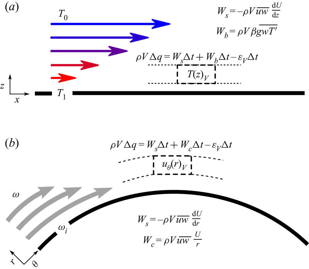
Figure 2. A schematic representation of the analogy between the effects of buoyancy and streamline curvature on a BL.  $(a)$ A flat plate unstably stratified BL. The change in energy production is governed by the work carried out on a volume element $V$ by buoyancy $W_b$ and shear $W_s$; $\beta$ is the thermal expansion coefficient, $g$ is the gravitational acceleration that is defined positive in the $-z$ direction, $T'$ is the temperate fluctuation and $\epsilon _V$ is the volumetric dissipation rate. $(b)$ A side view of a BL over a curved surface (or the top view of TC IC). In analogy to positive work carried out by buoyancy fluctuations in an unstably stratified thermal BL $(a)$, the rate of work done by centrifugal forces $W_c$ in the case of IC rotation is also positive.
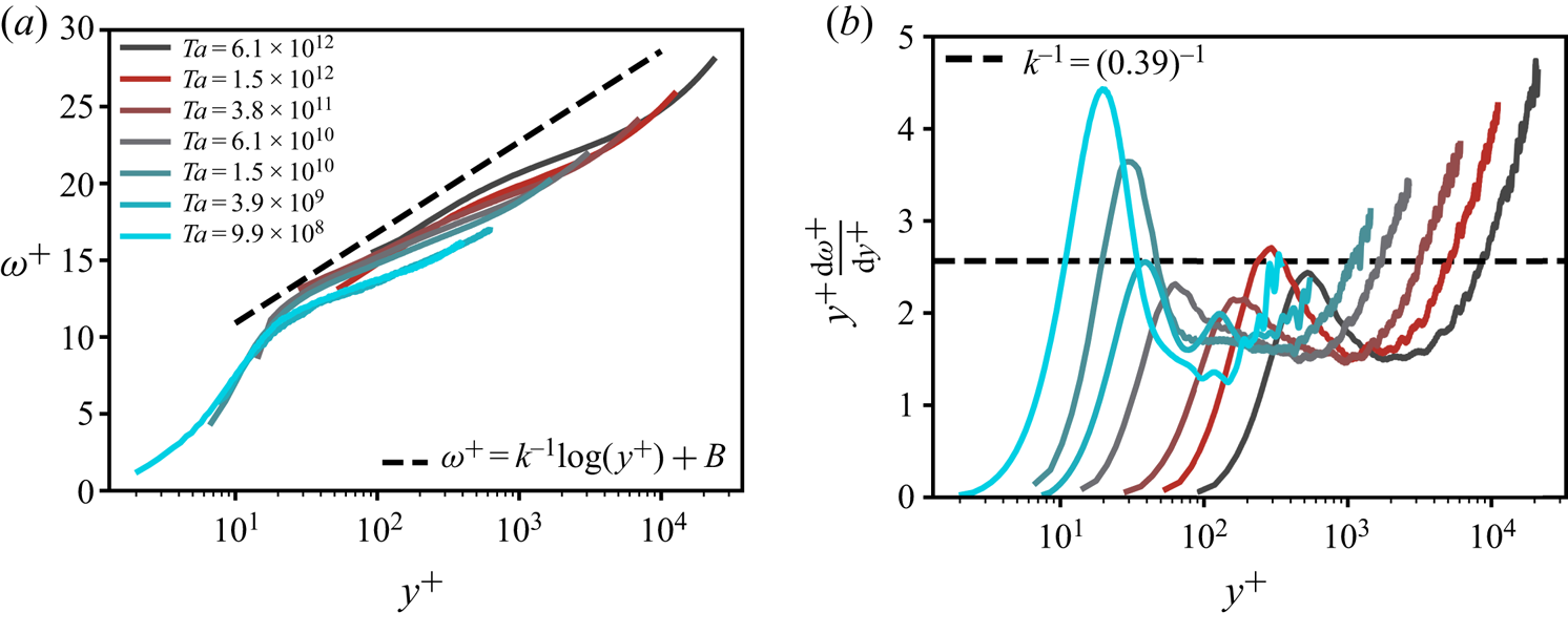
Figure 3. The IC BL angular velocity profiles for  $\eta =0.716$. $(a)$ Mean angular velocity $\omega ^{+} = (\omega _i-\langle \omega (r)\rangle _{A(r),t})/\omega _{\tau ,i}$ versus the wall-normal distance $y^{+}=(r-r_i)/\delta _{\nu ,i}$. A logarithmic velocity profile with slope $\kappa ^{-1}$ is observed in a limited spatial region at the highest Taylor numbers. $(b)$ The diagnostic function reveals a very limited spatial region in which $y^{+}({\textrm {d}\omega ^{+}}/{\textrm {d}y^{+}})=\kappa ^{-1}$, indicated by the dashed line. Data from the PIV measurements of Huisman et al. (Reference Huisman, Scharnowski, Cierpka, Kähler, Lohse and Sun2013).
4.2. Development of the functional form of $\omega ^{+}(y^{+})$

Figure 3(a) shows the angular velocity profiles for turbulent TC flow. For very high  $Re$ of $O(10^{6})$, Huisman et al. (Reference Huisman, Scharnowski, Cierpka, Kähler, Lohse and Sun2013) observed the existence of a logarithmic form of the angular velocity profile with $\kappa \approx 0.39$ and $B\approx 5$, in accordance with (4.1). However, the extent of the profile is very limited, namely $50<y^{+}<600$, covering a much smaller spatial range than it would in canonical wall-turbulence systems such as channel flow and flat plate turbulent boundary layers (Pope Reference Pope2000) at similar $Re_{\tau }$. Figure 3(b) presents the so-called diagnostic function, $y^{+}({\textrm {d}\omega ^{+}}/{\textrm {d}y^{+}})$, which allows for a more detailed investigation of the log slope of $\omega ^{+}(y^{+})$. Even for these high $Re$ flows, only a very small region of the profile coincides with the straight line with slope $\kappa ^{-1}$, which in this representation represents the log layer.
Following the analysis in § 4.1, we expect the velocity profile to behave differently in the region where curvature effects play a role – in close analogy with the Monin–Obukhov similarity theory. Therefore, we plot the compensated gradient of the velocity profile versus the ratio of turbulence production terms, see (4.6), in figure 4(a). For clarity we include only the highest three  $Ta$ number cases from the dataset of Huisman et al. (Reference Huisman, Scharnowski, Cierpka, Kähler, Lohse and Sun2013). Indeed, we find that the gradient of the velocity correlates strongly with the relative effects of shear and curvature. Where turbulence production is governed by shear alone, we find that the gradient approximates $\kappa ^{-1}$, albeit marginally. However, where curvature effects become significant, i.e. for $10^{0} \leq ({r}/{U})({\textrm {d}U}/{\textrm {d}r}) \leq 10^{1}$, we find that the gradient is $\lambda ^{-1}$. It is remarkable that the gradient is constant over such an extended range over which the relative effects of curvature and shear change. For $({r}/{U})({\textrm {d}U}/{\textrm {d}r}) \leq 10^{0}$ curvature effects are dominant and the bulk velocity profile sets in (see § 4.3).
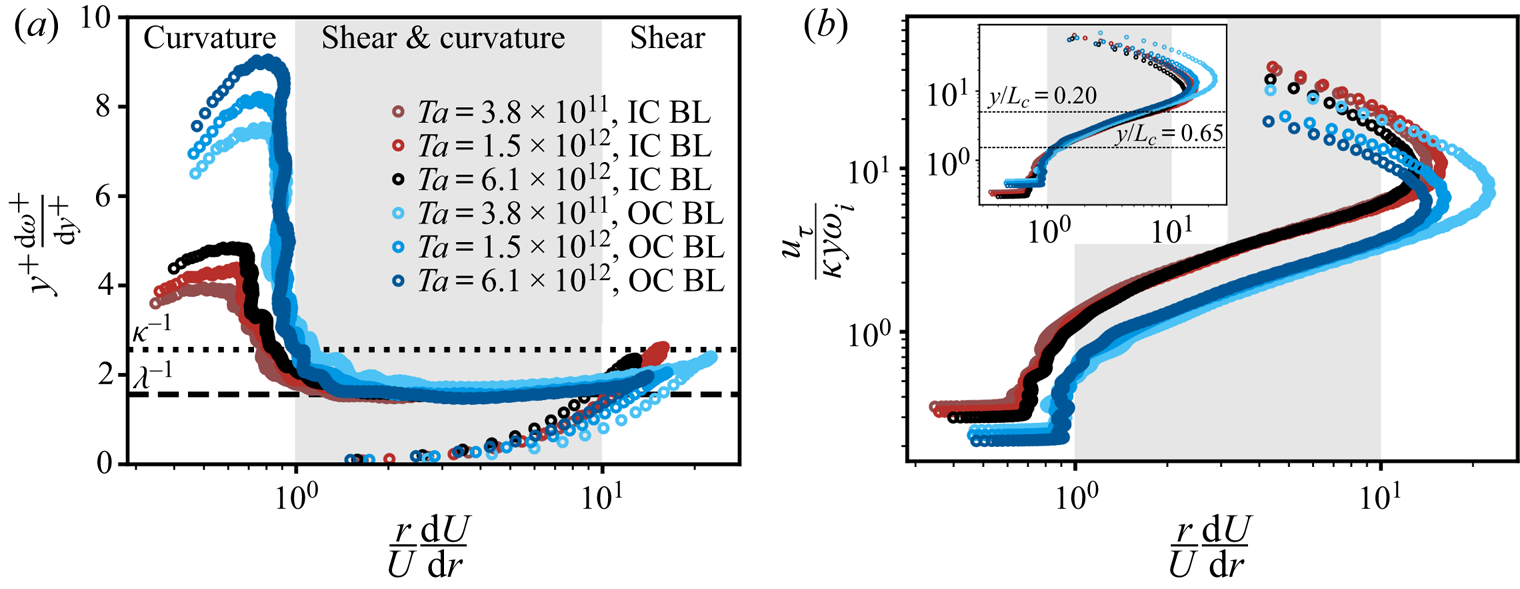
Figure 4.  $(a)$ Compensated gradient of the mean angular velocity versus the ratio of shear production of turbulence over curvature production of turbulence (see (4.6)). $(b)$ The approximation of the Obukhov curvature length $L_c(y)$ (4.7) versus the exact calculation of the Obukhov curvature length (4.6). Inset of $(b)$ highlights the collapse of IC and OC approximations with the use of different velocity scales (axis labels are the same as figure b), respectively $\omega _ir_i$ for the IC and $0.50\omega _ir_i$ for OC. Data from the PIV measurements of Huisman et al. (Reference Huisman, Scharnowski, Cierpka, Kähler, Lohse and Sun2013).
Consequently, we make the wall-normal distance dimensionless with  $L_c$, see (4.7). This is done in figure 5(b) where we plot the diagnostic function versus $y/L_c$. Similar to figure 4, we find a collapse of the angular velocity profiles, directly justifying the use of $L_c$ in turbulent TC flow. The profiles not only collapse with respect to their wall-normal location, but also all plateau at $y^{+}({\textrm {d}\omega ^{+}}/{\textrm {d}y^{+}})=\lambda ^{-1}$, i.e. the slope (in a semi-logarithmic representation) of $\omega ^{+}(y^{+})$. This secondary flat regime with slope $\lambda ^{-1}$ exists for larger $r>L_c$, than the $\kappa ^{-1}$ regime. We find that $\lambda =0.64$.
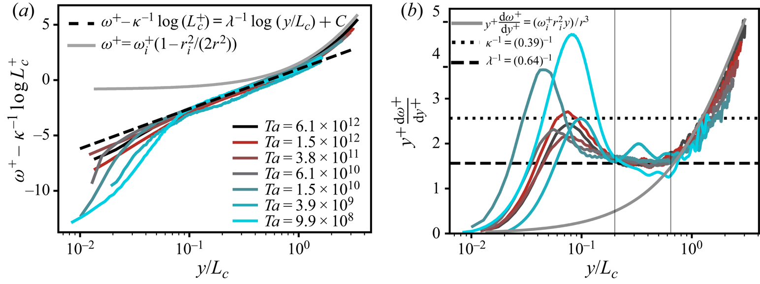
Figure 5. The IC BL mean angular velocity profiles for  $\eta =0.716$. $(a)$ Mean angular velocity $\omega ^{+} = (\omega _i-\langle \omega (r)\rangle _{A(r),t})/\omega _{\tau ,i}$ with the $L_c^{+}$ dependent offset $\kappa ^{-1}\log {(L_c^{+})}$ subtracted to highlight collapse of the profiles. The curved, thick, grey line is the constant angular momentum $M_{o}=\omega _ir_i^{2}/2$, as derived by Townsend (Reference Townsend1956), which very closely fits the data at $y>L_c$. $(b)$ Diagnostic function versus the rescaled wall-normal distance $y/L_c=(r-r_i)/L_c$, where $L_c=u_{\tau ,i}/ (\kappa \omega _i)$ is the curvature Obukhov length. The vertical grey lines indicate the bounds of the second log region. Data from the PIV measurements of Huisman et al. (Reference Huisman, Scharnowski, Cierpka, Kähler, Lohse and Sun2013).
From these observations in figure 5 we obtain the unknown function  $\varPhi _{\omega }({y}/{L_c})$ in (1.3) for $0.20<y/L_c<0.65$
 \begin{equation} \varPhi_{\omega} \left( \frac{y}{L_c} \right) = \frac{1}{\lambda} \approx \frac{1}{0.64}; \quad 0.20\lesssim y/L_c \lesssim 0.65. \end{equation}
Consequently, we integrate  ${\textrm {d}\omega ^{+}}/{\textrm {d}(y/L_c)}={1}/{(y/L_c)\lambda }$ and arrive at
 \begin{equation} \omega^{+} = \lambda^{-1}\log{(y/L_c)} + K, \end{equation}
where  $K$ is an integration constant and $\log$ is the natural logarithm. The offset $K$ of this second regime at larger $r$ is related to the height at which the first logarithmic regime at smaller $r$ peels off to the second log regime. We thus expect that $K = \kappa ^{-1}\log {L_c^{+}} + C$ which results in,
 \begin{equation} \omega^{+} = \lambda^{-1}\log{(y^{+})} + (\kappa^{-1}-\lambda^{-1})\log(L_c^{+}) + C, \end{equation}
where  $C$ is a constant equal to $1.0$ (obtained by fitting to the highest Taylor number data). If the transition from a shear logarithmic regime (with slope $\kappa ^{-1}$) to a curvature logarithmic regime (with slope $\lambda ^{-1}$) occurs exactly at $y^{+}=L_c^{+}$, and if this transition is sharp, we would expect to recover the offset of the curvature logarithmic regime as $K=\kappa ^{-1} \log L_c^{+} + B$. Hence, we would obtain the constant $C=B=5$. However, we see in figure 3(a) that the transition between the two logarithmic regions in the flow is not sharp, but gradual. The gradual transition from the shear-dominated region to the curvature affected region and the long ‘blending’ region in between made us decide not to simply equate (4.10) with the von Kármán profile to obtain the lower bound of the curvature logarithmic region (4.8). Instead, as explained, we employ a stricter empirical condition from which we find $y=0.20L_c$. In figure 5(a) we plot $\omega ^{+}$ versus $y/L_c$ and subtract $K$ to highlight the collapse. Indeed, we observe a collapse of the profiles in the range $0.20\lesssim y/L_c \lesssim 0.65$.
4.3. The constant angular momentum region in the bulk
In the previous section we discussed the shape of the mean streamwise velocity profile in the IC BL, culminating in a new functional form which includes the stratification length  $L_c$. However, to arrive at a $Nu(Ta)$ relationship, we need to assess the velocity profile in the bulk region, too. Wendt (Reference Wendt1933) already observed that for unstable flows (i.e. IC rotation and a stationary OC) the bulk flow obeys a constant angular momentum ${L}={M}_{o}$. Later, Townsend (Reference Townsend1956) came to a similar conclusion and found that ${M}_{o} = \omega _ir_i^{2}/2$ for pure IC rotation. In recent years this finding is often confirmed by new datasets, see e.g. Ostilla-Mónico et al. (Reference Ostilla-Mónico, Verzicco, Grossmann and Lohse2015a), Brauckmann, Salewski & Eckhardt (Reference Brauckmann, Salewski and Eckhardt2016) and Cheng et al. (Reference Cheng, Pullin and Samtaney2020). This region of constant angular momentum in IC rotating TC flow is reminiscent to a linear mean flow scaling in the bulk of spanwise rotating channel flow (Johnston et al. Reference Johnston, Halleent and Lezius1972; Nakabayashi & Kitoh Reference Nakabayashi and Kitoh1996; Yang et al. Reference Yang, Xia, Lee, Lv and Yuan2018).
Here, we plot the constant angular momentum region in figure 5. We find that the transition from a  $\lambda ^{-1}$ region into a constant angular momentum $\omega ^{+} = \omega _i^{+}(1-r_i^{2}/(2r^{2}))$ region occurs at $y=L_c$. As such, the bulk region is entirely dominated by curvature effects of the streamlines. Consequently, the IC BL thickness $\delta _i$ is equal to the curvature Obukhov length, $\delta _i \approx L_c$ (and OC BL thickness $\delta _o= 2.5 L_c$). Recently, a very similar thickness of the BL was empirically found by Cheng et al. (Reference Cheng, Pullin and Samtaney2020).
4.4. The outer cylinder boundary layer
Analogous to the IC BL we can analyse the OC BL, with IC rotation only, in the spirit of the Monin–Obukhov similarity theory. As mentioned in § 4, Huisman et al. (Reference Huisman, Scharnowski, Cierpka, Kähler, Lohse and Sun2013) also obtained velocity profiles of the OC BL for the highest five  $Ta$ number experiments. From (4.6) we derive that the relevant length scale for the OC BL is $L_{c,o} = r u_{\tau ,o}/(\kappa U)$ with $y=r_o-r$. We approximate the velocity $U$ with the scale $\omega _ir_i$ and the radius of curvature $r$ with $r_o$, so that with $u_{\tau , o}r_o = u_{\tau , i}r_i$, $L_{c,o}=u_{\tau ,i}/(\kappa \omega _i)$. The length scale is the same as $L_{c,i}$.
The definition of the Obukhov curvature length  $L_c = (u_{\tau ,i}r_i)/(\kappa U)$ contains a velocity $U$. Although this velocity is a function of the wall-normal coordinate, we approximate it by the velocity scale $u_i$ of the IC throughout. The difference between the actual velocity in the IC boundary layer and $u_i$ is different from the difference between the actual velocity in the outer cylinder boundary layer and $u_i$. In figure 4(b) we find that indeed the approximation of $L_c$ in (4.7) is not consistent for IC and OC when we employ $U=\omega _ir_i$. However, the inset shows that when we use $U=0.50\omega _i r_i$ as the velocity scale for the OC (and $U=\omega _ir_i$ for the IC), the approximation of $L_c$ is consistent.
Figure 6(b) presents the gradient of the OC BL velocity profiles versus the dimensionless wall distance  $y/L_c$. Again, we observe collapse of the profiles in both the vertical direction and the horizontal direction. In the range $0.20<y/L_c<0.65$ the gradient of the profiles is $\lambda ^{-1}$, whose value is identical to the IC BL profiles. Since the findings in figure 6(b) are the same as in figure 5(b), we derive the velocity profile for the OC BL in the same manner as ((4.8)–(4.10)) and arrive at
 \begin{equation} \omega^{+}_o = \lambda^{-1}\log{(y^{+})} + (\kappa^{-1}-\lambda^{-1})\log(L_c^{+}) + C_o, \end{equation}
where  $C_o=2.0$ is obtained from fits in figure 6(a). Again, the profiles in figure 6(a) exhibit fair overlap between (4.11) and the experimental data, especially at the highest two $Ta$ numbers (see inset). We note that $Re_{\tau ,o}$ at the OC BL is smaller than $Re_{\tau ,i}$ at the IC BL, and consequently, we expect that the data at lower $Ta$ still suffer from insufficient scale separation.
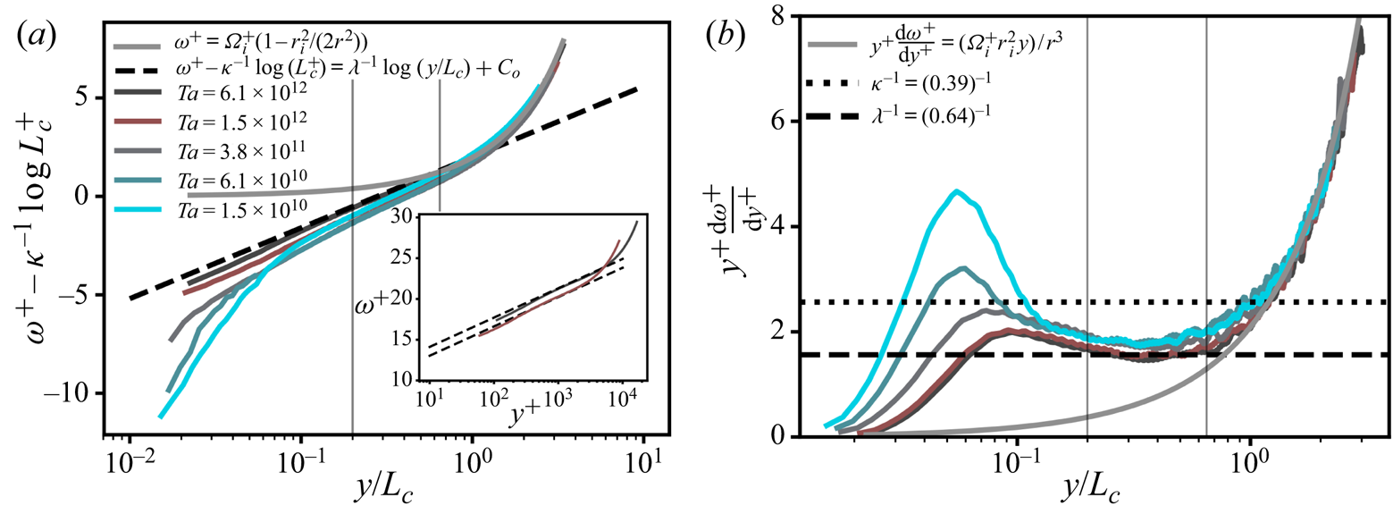
Figure 6. The OC BL angular velocity profiles for  $\eta =0.716$. $(a)$ Mean angular velocity $\omega ^{+} = \langle \omega (r)\rangle _{A(r),t}/\omega _{\tau ,o}$ with the $L_c^{+}$ dependent offset $\kappa ^{-1}\log {L_c^{+}}+C_o$ subtracted to convey collapse of the profiles. The vertical grey lines indicate the bounds of the second log region. The curved, thick, grey line is the constant angular momentum ${M}_{o}=\omega _ir_i^{2}/2$, as derived by Townsend (Reference Townsend1956), which very closely fits the data at $y>L_c$. $(b)$ Diagnostic function versus the rescaled wall-normal distance $y/L_c=(r_o-r)/L_c$, where $L_c=u_{\tau ,i}/ (\kappa \omega _i)$ is the curvature Obukhov length. For lower $y$ (
$y$ ( $y<0.20L_c$) the shear-dominated logarithmic regime with slope $\kappa ^{-1}$ peels off into a second logarithmic regime with slope $\lambda ^{-1}$. The inset to $(a)$ shows the mean angular velocity versus the wall-normal distance $y^{+}=(r_o-r)/\delta _{\nu ,o}$, where the dashed line is the curvature logarithmic relation. Data from the PIV measurements of Huisman et al. (Reference Huisman, Scharnowski, Cierpka, Kähler, Lohse and Sun2013).
5. The effects of the radius ratio $\eta$

Up to this point, we have shown that one can treat IC rotating TC flow as an unstably stratified turbulent shear flow, in close analogy with temperature stratified flows. We proposed a new functional form of the mean angular velocity in (4.10) that well describes the experimental profiles measured by Huisman et al. (Reference Huisman, Scharnowski, Cierpka, Kähler, Lohse and Sun2013) in both inner and outer BL for all  $Re$ at $\eta =0.716$. The question arises what the implications of the theory of stratified flows – and consequently (4.10) – bring to TC turbulence at varying radius ratios. To answer this question we first analyse DNS data of Ostilla-Mónico et al. (Reference Ostilla-Mónico, Verzicco, Grossmann and Lohse2015a) and PIV data of van der Veen et al. (Reference van der Veen, Huisman, Merbold, Harlander, Egbers, Lohse and Sun2016) at a lower radius ratio of $\eta =0.50$ (corresponding to larger curvature effects), followed by the analysis of the DNS Ostilla-Mónico et al. (Reference Ostilla-Mónico, Verzicco, Grossmann and Lohse2015a) data at a high radius ratio of $\eta =0.909$.
5.1. Radius ratio $\eta =0.5$

Figure 7 presents the velocity profiles at  $\eta =0.5$. The black solid line represents DNS data at a remarkable high $Ta$ of $1.1\times 10^{11}$ resulting in a significant scale separation; $Re_{\tau } = 3257$, see table 1. Nevertheless, the diagnostic function in figure 7(b) does not portray a shear-dominated $\kappa ^{-1}$ regime, i.e. the solid black line never follows the black dotted line. However, between $y/L_c\approx 0.20$ and $y/L_c\approx 0.65$ the $\lambda ^{-1}$ regime is obtained. Note that we do not fit $\lambda ^{-1}$ to the data, but only use the value ( $\lambda =0.64$) as obtained in § 4. The dark grey solid line departs from the $\lambda ^{-1}$ region around $y/L_c\approx 0.65$, to follow the ${M}_{o}=\omega _ir_i^{2}/2$ scaling of the bulk. This is in agreement with the observations at $\eta =0.716$.
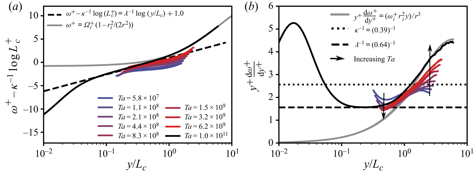
Figure 7. The IC BL mean angular velocity profile at  $\eta =0.50$. $(a)$ Mean angular velocity $\omega ^{+} = (\omega _i-\langle \omega (r)\rangle _{A(r),t})/\omega _{\tau ,i}$ with the $L_c^{+}$ dependent offset $\kappa ^{-1}\log {(L_c^{+})}$ subtracted to convey collapse of the profiles. The curved, thick, grey line is the constant angular momentum ${M}_{o}=\omega _ir_i^{2}/2$, as derived by Townsend (Reference Townsend1956), which very closely fits the data at $y>L_c$. The black solid line represents DNS data of Ostilla-Mónico et al. (Reference Ostilla-Mónico, Verzicco, Grossmann and Lohse2015a) whereas the coloured lines represent the PIV data by van der Veen et al. (Reference van der Veen, Huisman, Merbold, Harlander, Egbers, Lohse and Sun2016). $(b)$ Diagnostic function versus the rescaled wall-normal distance $y/L_c=(r-r_i)/L_c$, where $L_c=u_{\tau ,i}/ (\kappa \omega _i)$ is the curvature Obukhov length.
To understand the absence of a  $\kappa ^{-1}$ region for this low $\eta$, we refer to the scale separation in table 1. A $\kappa ^{-1}$ slope requires that $30 < y^{+} \ll 0.20L_c^{+}$. However, for $\eta =0.50$ at $Ta=1.1\times 10^{11}$ we find that $0.20L_c^{+} = 109$. This marginal scale separation is insufficient to find a logarithmic velocity profile with slope $\kappa ^{-1}$. However, the scale separation seems to be sufficient to determine the offset of the curvature logarithmic part of the velocity profile, i.e. $K=1/\kappa \log (L_c^{+}) + 1.0$ in (4.9) shown in figure 7(a). A large separation of scales between $L_c^{+}$ and $Re_{\tau }$ results in a large curvature-dominated flow region where the angular momentum becomes constant, see figure 7(a).
Figure 7 also presents PIV data for low  $Ta$ from van der Veen et al. (Reference van der Veen, Huisman, Merbold, Harlander, Egbers, Lohse and Sun2016). Although the scale separation is limited for $Re_{\tau }<1000$ we find a that with increasing $Ta$ the profiles convergence to the $\lambda ^{-1}$ region. For the very low Taylor number cases, the offset is too low to reach the dashed line, indicating that the shear logarithmic region is absent. This is confirmed by the absence of sufficient scale separation (i.e. $0.2L_c^{+}<30$, with $y^{+}=30$ the conventional start of the shear logarithmic region (Pope Reference Pope2000)) to form a shear logarithmic regime, see table 1 in the appendix. However, for $0.2L_c^{+}>30$ (at $Ta \ge 3.2\times 10^{9}$), the offset of the curvature region is correctly set by the shear velocity logarithmic profile. Hence, the profiles follow the prediction.
5.2. Radius ratio $\eta =0.909$

Figure 8 shows data from a DNS at high  $\eta =0.909$ (corresponding to small curvature effects) and $Ta = 1.0\times 10^{11}$. Interestingly, we observe a pronounced $\kappa ^{-1}$ region. However, there is a total absence of the $\lambda ^{-1}$ and the ${M}_{o}$ region. Once again this is understood with the scale separation argument. In this case $L_c^{+}>Re_{\tau }$, and therefore there is no location in the flow where the curvature effects are significant, see table 1.
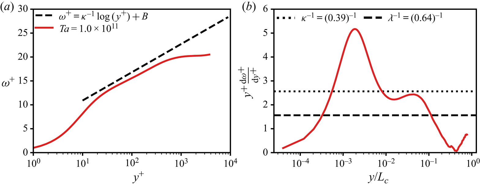
Figure 8.  $(a)$ Mean angular velocity $\omega ^{+} = (\omega _i-\langle \omega (r)\rangle _{A(r),t})/\omega _{\tau ,i}$ versus the wall-normal distance $y^{+}$. The red solid line is DNS data taken from Ostilla-Mónico et al. (Reference Ostilla-Mónico, Verzicco, Grossmann and Lohse2015a). $(b)$ Diagnostic function versus the rescaled wall-normal distance $y/L_c=(r-r_i)/L_c$, where $L_c=u_{\tau ,i}/ (\kappa \omega _i)$ is the curvature Obukhov length, for $\eta =0.909$.
5.3. General radius ratio $\eta$

To close this section, we provide a phase diagram of the scale separation at  $Re_{\tau }\approx 3000$ for varying $\eta$, in order to illustrate where one would expect to see $\kappa ^{-1}$, $\lambda ^{-1}$, and constant angular momentum regions of the angular velocity profile, in figure 9. We base the phase diagram on three cases for $\eta =(0.500, 0.716, 0.909)$ and $Re_{\tau }\approx 3000$, for which we have the phase boundaries, see table 1. Note that the boundaries are not sharp, and gradual changes in the relative importance of TKE production by shear and curvature lead to new regions. However, we now immediately see from the diagram that, for high $\eta$, the Obukhov curvature BL is only expected to appear distinctly at extremely high $Re_{\tau }$ (higher than $Re_{\tau }=3000$). In contrast, for low $\eta$, we need extremely high $Re_{\tau }$ (higher than $Re_{\tau }=3000$) to observe the Prandtl–von Kármán turbulent BL type.
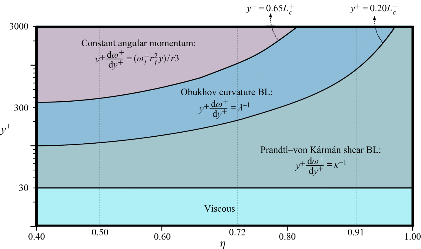
Figure 9. Varying regimes in between the solid boundary (here the IC wall at  $y^{+}=0$) and the outer length scale at $y^{+}=Re_{\tau }$ for increasing radius ratio $\eta$, from $\eta =0.4$ (strong curvature) to $\eta =1.0$ (no curvature). The diagram is based on the values of $L_c^{+}$ at $Re_{\tau }\approx 3000$ for $\eta =(0.500, 0.716, 0.909)$, see table 1 in the appendix.
6. The $Nu(Ta)$ and ${C}_{f}(Re_{i})$ relationships


The derivation of the angular velocity profile in a turbulent BL with strong curvature effects, see (4.10), allows us to obtain a functional form that relates the dimensionless torque  $Nu$ to the dimensionless driving $Ta$ at $Re_o=0$. To do so, we follow the very recent work by Cheng et al. (Reference Cheng, Pullin and Samtaney2020). Therein, the BL profile (the conventional shear-dominated von Kármán type) is matched with the constant angular momentum bulk profile at the edge of the BL. With a fitting constant for the BL thickness, Cheng et al. (Reference Cheng, Pullin and Samtaney2020) arrive at a very accurate calculation of $Nu$ over a wide range of $Ta$. Here, we match the angular velocity profiles in the bulk and the BL at the BL height $\delta = \alpha L_c$. Note that the constant $\alpha$ is easily extracted from figure 5, where it refers to the outer bound of the $\lambda ^{-1}$ region – where the BL and bulk meet.
 \begin{equation} \frac{\omega_i}{\omega_{\tau,i}} - \frac{1}{\lambda}\log \alpha L_c^{+} - \left(\frac{1}{\kappa}-\frac{1}{\lambda}\right) \log L_c^{+} - C = \frac{\omega_ir_i^{2}}{2\omega_{\tau,i}(r_i+\alpha L_c)^{2}}. \end{equation}
Note that (6.1) is equivalent to Cheng et al. (Reference Cheng, Pullin and Samtaney2020) ((4.5)–(4.7)) with differences of  $O(Re_{\tau }/Re_i)$, and with a different constant. Upon closely following Cheng et al. (Reference Cheng, Pullin and Samtaney2020) including $Re_{\tau } \ll Re_i$, (6.1) results,
 \begin{equation} Nu = \frac{\kappa^{2} \eta^{3} Ta^{1/2}}{4(1+\eta)^{2} W(Z)^{2}}, \quad Z= \sqrt{\frac{\kappa \eta^{3} Ta^{1/2}}{2(1-\eta)(1+\eta)^{3}}}\exp{\left(\frac{\kappa \left( C+\dfrac{1}{\lambda}\log \alpha \right) }{2}\right)}, \end{equation}
where  $W(Z)$ is the principal branch of the Lambert $W$ function. We note that (6.2a,b) is different from the result of Cheng et al. (Reference Cheng, Pullin and Samtaney2020) ((4.15)–(4.16)) by only a constant in the argument of the productlog function and the difference in $Nu(Ta)$ is only minor. We refer to (6.2a,b) as the ‘present CPS model’ (i.e. p-CPS).
Figure 10 presents (6.2a,b) together with 8 datasets from DNS and experiments – covering  $0.357 \le \eta \le 0.909$ and 7 orders of magnitude in $Ta$;
$Ta$;  $\alpha =0.65$, see (4.8) and figure 5. Naturally, we find deviations at low $Ta$, where the BLs are not fully turbulent yet. However, we find good overlap at high $Ta$ for various $\eta$. For high $\eta$ (at $Re_{\tau }=3000$, $\eta \gtrsim 0.80$), (6.2a,b) loses its validity since shear is dominating curvature effects throughout the entire BL at the current $Ta$. The $Nu(Ta)$ relation is thus better described by the functional form obtained in Cheng et al. (Reference Cheng, Pullin and Samtaney2020). However, we note that the ratio $Re_{\tau }/L_c^{+}$ will become larger with increasing $Ta$, so that for extremely high $Ta$ (even much higher than $10^{12}$), the $Nu(Ta)$ relationship at $\eta =0.909$ will also follow (6.2a,b).
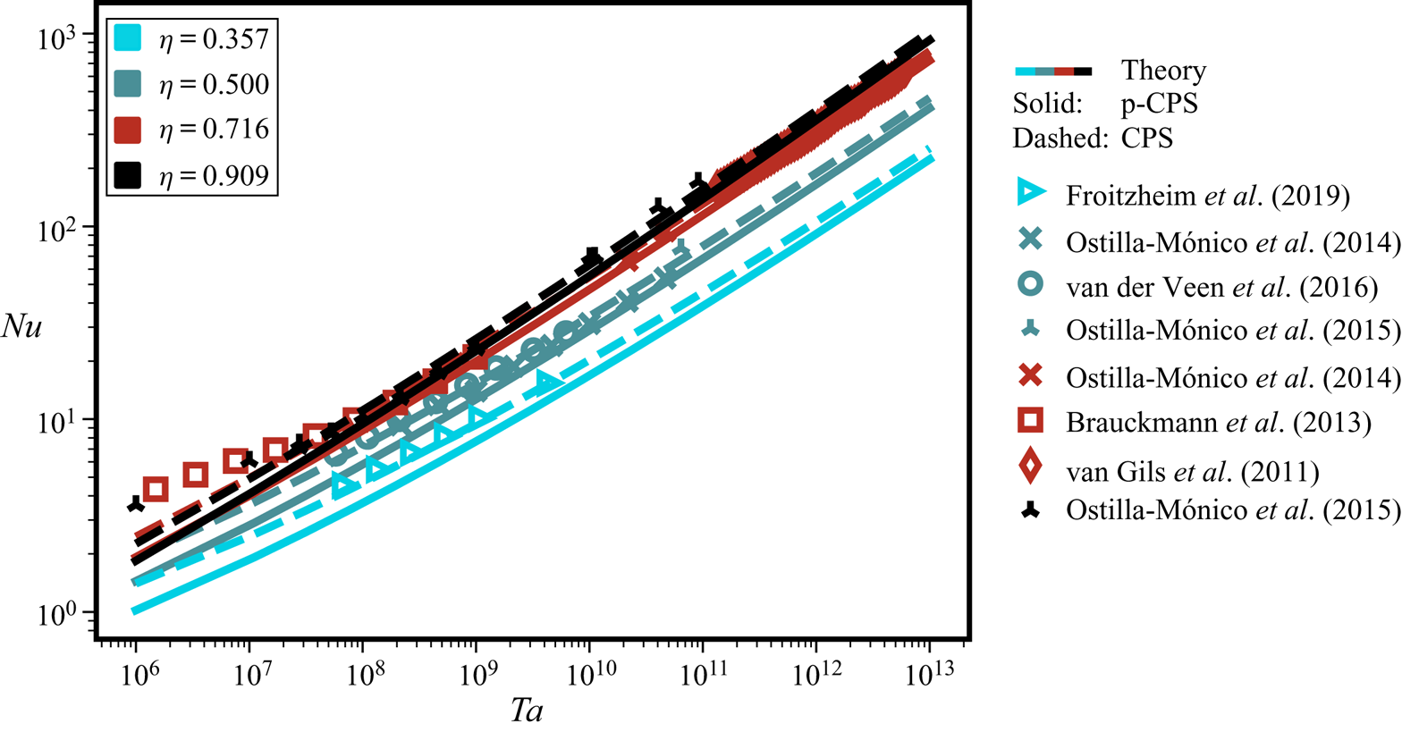
Figure 10. The dimensionless torque  $Nu$ versus the dimensionless rotation rate $Ta$ of the IC. Solid lines represent the result as obtained by the matching of profiles in § 6, with the resulting relationship $Nu(Ta)$ given by (6.2a,b) (present p-CPS). Dashed lines represent the result of Cheng et al. (Reference Cheng, Pullin and Samtaney2020) (CPS). Symbols are the values of $Nu$ obtained by DNS or experiments; $\eta =0.357$ (blue triangle) Froitzheim et al. (Reference Froitzheim, Merbold, Ostilla-Mónico and Egbers2019), $\eta =0.500$ (crosses) Ostilla-Mónico et al. (Reference Ostilla-Mónico, van der Poel, Verzicco, Grossmann and Lohse2014b), (open circles) van der Veen et al. (Reference van der Veen, Huisman, Merbold, Harlander, Egbers, Lohse and Sun2016) and (triangle) Ostilla-Mónico et al. (Reference Ostilla-Mónico, Verzicco, Grossmann and Lohse2015a), $\eta =0.716$ (squares) Brauckmann & Eckhardt (Reference Brauckmann and Eckhardt2013), (crosses) Ostilla-Mónico et al. (Reference Ostilla-Mónico, van der Poel, Verzicco, Grossmann and Lohse2014b) and (diamonds) van Gils et al. (Reference van Gils, Huisman, Bruggert, Sun and Lohse2011b), $\eta =0.909$ (triangles) Ostilla-Mónico et al. (Reference Ostilla-Mónico, Verzicco, Grossmann and Lohse2015a).
For  $Ta<10^{6}$, the BLs are of the laminar type and $Nu$ scales with $Ta^{1/3}$ (Ostilla-Mónico et al. Reference Ostilla-Mónico, van der Poel, Verzicco, Grossmann and Lohse2014a). Figure 11(a) shows the $Nu(Ta)$ relationship where $Nu$ is compensated with $Ta^{1/3}$, such that we highlight the transition to a turbulent BL where the scaling exponent is larger than ${1/3}$. We emphasize that, only after this transition, which is gradual and appears to depend on $\eta$, when BLs are entirely turbulent, will (6.2a,b) correctly calculate $Nu(Ta)$. Figure 11(b) presents the ${C}_f(Re_i$) diagram, which is more conventionally used in the pipe flow and BL flow communities. The solid lines are given by (6.2a,b) where the friction factor is calculated from $C_f = 4Nu/(\eta (1+\eta )Re_i)$.
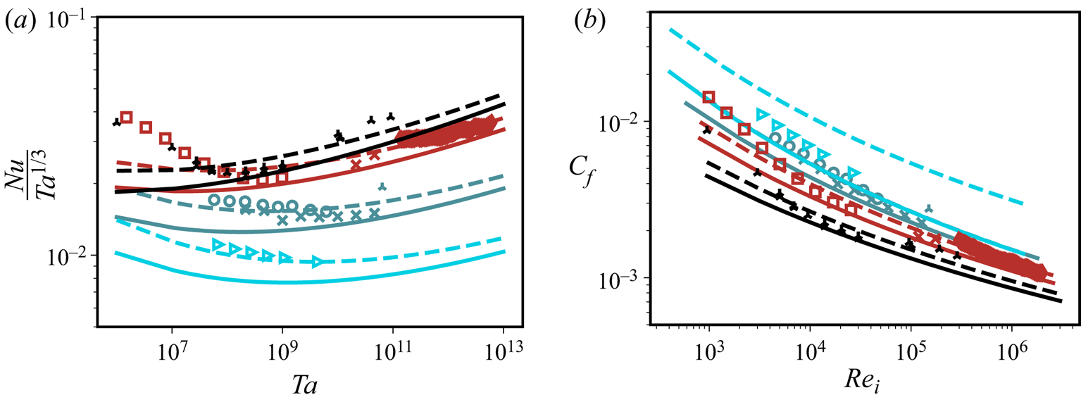
Figure 11.  $(a)$ The dimensionless torque $Nu$, compensated with the scaling of TC flow with laminar BL and turbulent bulk $Ta^{1/3}$, versus the dimensionless rotation rate $Ta$ of the IC. $(b)$ The friction factor $C_f$ versus the the IC Reynolds number $Re_i$. Colours and symbols are the same as in figure 10 and links to the references can be found in the caption of that figure.
7. Summary and conclusions
In summary, we have developed a theory, similar to that of thermally stratified turbulent BLs, as famously developed by Monin & Obukhov (Reference Monin and Obukhov1954), for the curved turbulent BLs in inner cylinder rotating TC flow. In this analogy, the destabilizing effects from curvature of the streamlines in inner cylinder rotating TC flow are similar to the destabilizing effects coming from unstable thermal stratification in the atmospheric BL.
We show that the curvature Obukhov length  $L_c$ (Bradshaw Reference Bradshaw1969) separates the spatial regions that are dominated by shear and curvature effects. We find that for $\delta _{\nu } < y \lesssim 0.20L_c$, the mean angular velocity profile in the BL is described by the classical shear profile, with the slope given by the von Kármán constant $\kappa ^{-1}=0.39^{-1}$. In contrast, for $0.20L_c \lesssim y \lesssim 0.65L_c$, where curvature effects are relevant, the slope of the angular velocity profile is $\lambda ^{-1}=0.64^{-1}$. For $y \gtrsim 0.65L_c$ curvature effects dominate, and a region with constant angular momentum sets in. This theory is applied to – and found consistent with – PIV measurements and high-fidelity DNS data covering a wide range of radius ratios $0.50 \le \eta \le 0.909$ and rotation rates $10^{8} \le Ta \le 10^{12}$, and describes both the IC BL and the OC BL.
Building on these findings we obtain a new functional form of the mean angular velocity profile in TC turbulence, with separate spatial regions where curvature and shear effects are respectively relevant. In implementing the Cheng et al. (Reference Cheng, Pullin and Samtaney2020) theory by matching our new outer boundary layer profile with the constant angular momentum profile in the bulk at the edge of the BL, we recover their  $Nu(Ta, \eta )$ (and $C_f (Re_i , \eta ))$ relations but with a different constant. For the present smooth-wall flow with the outer cylinder stationary, this supports their model, with fair agreement with various datasets at high $Ta$ and different $\eta$.
The key assumptions made by Bradshaw (Reference Bradshaw1969), namely that the net production of turbulent kinetic energy is locally balanced by dissipation, as also employed in this research, are left to be addressed by means of DNS at very high Reynolds numbers of  $Re=O(10^{6})$. Whether the Obukhov (outer) logarithmic region will survive at arbitrary high $Re_i$ remains an open question. Open questions also concern the effects of stably stratified TC flow (i.e. outer cylinder rotation), or even mixed stratified TC flow (i.e. counter cylinder rotation) within the framework of the Monin–Obukhov similarity theory. However, so far, only velocity profiles with a scale separation up to $Re_{\tau }\approx 1200$ are available for OC rotation (Ostilla-Mónico, Verzicco & Lohse Reference Ostilla-Mónico, Verzicco and Lohse2016) to apply the theoretical analysis. Also, based on the newly derived velocity profile, it becomes necessary to reassess the fully rough asymptote for rough wall turbulent TC flow (Berghout et al. Reference Berghout, Zhu, Chung, Verzicco, Stevens and Lohse2019).
Acknowledgements
This paper is devoted to Professor S. Grossmann on occasion of his 90th birthday. We congratulate him and thank him for all we learned from him on turbulence, physics, science, and beyond. We are very grateful to S. Huisman, R. Ostilla-Mónico and R. van der Veen for providing us their data. We further thank I. Marusic, D. Krug, N. Hutchins, M. Bruning, and D. Pullin for insightful discussions. This project is funded by the Priority Programme SPP 1881 Turbulent Superstructures of the Deutsche Forschungsgemeinschaft. R.S. acknowledges financial support from the European Research Council through starting grant no. 804283 UltimateRB.
Declaration of interests
The authors report no conflict of interest.
Appendix
See table 1 for an overview of the used datasets and figure 12 for an application of the analysis to the azimuthal velocity profile.
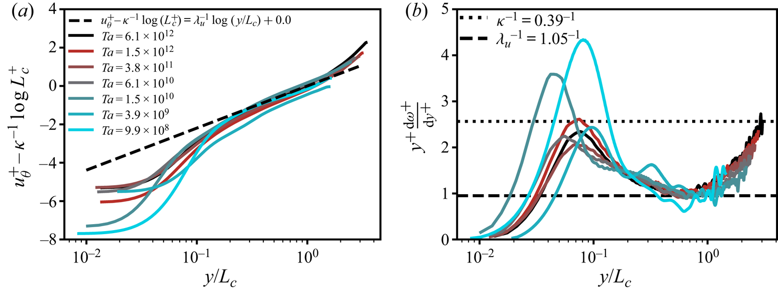
Figure 12. The inner cylinder BL mean azimuthal velocity profiles for  $\eta =0.716$. $(a)$ Mean azimuthal velocity $u_{\theta }^{+} = (u_{\theta ,i}-\langle u_{\theta }(r)\rangle _{A(r),t})/u_{\tau ,i}$ with the $L_c^{+}$ dependent offset $\kappa ^{-1}\log {(L_c^{+})}$ subtracted to highlight collapse of the profiles. $(b)$ Diagnostic function versus the rescaled wall-normal distance $y/L_c=(r-r_i)/L_c$, where $L_c=u_{\tau ,i}/ (\kappa \omega _i)$ is the curvature Obukhov length. Note that $\lambda _u^{-1}$ is different than $\lambda ^{-1}$ in the main text. Data from the PIV measurements of Huisman et al. (Reference Huisman, Scharnowski, Cierpka, Kähler, Lohse and Sun2013).


 Open access