


1 Introduction
In a horizontal convection (HC) system, heating and cooling take place over a single horizontal surface of a fluid layer. Sandstrom (Reference Sandstrom1908) argued that, due to the absence of a pressure gradient, a closed circulation cannot be maintained in such systems. However, six decades later, Rossby (Reference Rossby1965) demonstrated in his experiments that HC alone, independent of any other sources, is able to create a circulation of a fluid and therefore a net convective buoyancy flux. Over the past decades, Rossby’s set-up has become a popular paradigm case to study this important type of natural convective system (Hughes & Griffiths Reference Hughes and Griffiths2008; Griffiths, Hughes & Gayen Reference Griffiths, Hughes and Gayen2013), which is relevant in geophysical flows like the meridional overturning circulation in the ocean (Munk Reference Munk1966; Killworth Reference Killworth1983; Scott, Marotzke & Adcroft Reference Scott, Marotzke and Adcroft2001; Cushman-Roisin & Beckers Reference Cushman-Roisin and Beckers2011; Scotti & White Reference Scotti and White2011), in astrophysical flows (Spiegel Reference Spiegel1971) and in engineering applications (Gramberg, Howell & Ockendon Reference Gramberg, Howell and Ockendon2007). Investigations of HC systems are also necessary for understanding the effect of polar amplification on the ocean circulation (Holland & Bitz Reference Holland and Bitz2003), i.e. a phenomenon of global warming that decreases the temperature contrast between the poles and mid-latitudes.
In any convective system, a naturally arising question is: How do the global heat transport (Nusselt number  $Nu$) and momentum transport (Reynolds number $Re$) depend on the main input parameters (Rayleigh number $Ra$ and Prandtl number $Pr$)? While considering a laminar boundary layer (BL) and balancing buoyancy and viscous dissipation terms inside the BL, Rossby (Reference Rossby1965) proposed a relation $Nu\sim Ra^{1/5}Pr^{0}$. The existence of the ${\sim}Ra^{1/5}$ regime was supported by various numerical and experimental studies (e.g. Mullarney, Griffiths & Hughes Reference Mullarney, Griffiths and Hughes2004; Gayen, Griffiths & Hughes Reference Gayen, Griffiths and Hughes2014), but the predicted $Pr$ invariance of $Nu$ does not hold for small $Pr$ (e.g. Shishkina & Wagner Reference Shishkina and Wagner2016). By considering the dynamics to be driven by a turbulent endwall plume, Hughes et al. (Reference Hughes, Griffiths, Mullarney and Peterson2007) proposed the scaling $Nu\sim Ra^{1/5}Pr^{1/5}$, but, as shown in Shishkina & Wagner (Reference Shishkina and Wagner2016), the proposed $Pr$ scaling is too strong and is not supported by direct numerical simulations (DNS). Whereas the Rossby model is based solely on the BL scalings, the model by Shishkina, Grossmann & Lohse (Reference Shishkina, Grossmann and Lohse2016) (Reference Shishkina, Grossmann and LohseSGL model), which is an extension of the Grossmann & Lohse (Reference Grossmann and Lohse2000, Reference Grossmann and Lohse2001, Reference Grossmann and Lohse2004) theory to HC, is able to account for laminar regimes as well as for regimes where the mixing is governed by turbulent processes. In particular, the Reference Shishkina, Grossmann and LohseSGL model suggests $Nu\sim Pr^{0}Ra^{1/4}$ for large- $Pr$ and $Nu\sim Pr^{1/10}Ra^{1/5}$ for small- $Pr$ laminar flows, which was supported by several numerical studies (Shishkina & Wagner Reference Shishkina and Wagner2016; Ramme & Hansen Reference Ramme and Hansen2019).
However, verification of the other regimes needs further investigations. For this, high- $Ra$ DNS or experiments are needed, which turn out to be challenging tasks. On the one hand, the very slow diffusion in the system is a critical problem for the DNS of (almost) steady flows. On the other hand, in experiments, unwanted heat losses through the vertical walls can affect the scaling results significantly (Ahlers Reference Ahlers2000). Therefore, in this work we focus on two set-ups: classical horizontal convection (CHC) and symmetrical horizontal convection (SHC), which can be more suitable for future experiments. Here we report three-dimensional (3-D) DNS results for $Ra\leqslant 3\times 10^{12}$ and $Pr=0.1$, 1 and 10.
2 Theoretical background
We consider a fluid layer that is confined in a rectangular box and heated and cooled locally from the bottom. In the CHC set-up, heating and cooling are applied to the opposite bottom ends (figure 1a); while in the SHC set-up, the bottom is cooled at the ends and heated in the central part (figure 1b). The advantage of the SHC set-up over the HC one is the absence of the vertical endwall attached to the heated plate, which is difficult to isolate thermally in experiments. For both set-ups, we conducted extensive 3-D DNS over the range of parameters shown in figure 1(c), where the DNS data for CHC and  $Ra<3\times 10^{11}$ are taken from Shishkina (Reference Shishkina2017).

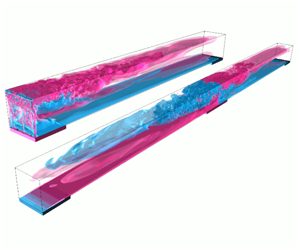
Figure 1. Sketch of (a) CHC and (b) SHC set-ups. Colours inside the cells represent the lengthwise velocity  $u_{x}$: $u_{x}>0$ (pink) and $u_{x}<0$ (blue). (c) The studied parameter range for CHC (closed symbols) and SHC (open symbols).
The governing equations in the Oberbeck–Boussinesq approximation for the dimensionless velocity  $\boldsymbol{u}$, temperature $\unicode[STIX]{x1D703}$ and pressure $p$ read as follows:
 $$\begin{eqnarray}\displaystyle & \displaystyle \unicode[STIX]{x2202}\boldsymbol{u}/\unicode[STIX]{x2202}t+\boldsymbol{u}\boldsymbol{\cdot }\unicode[STIX]{x1D735}\boldsymbol{u}+\unicode[STIX]{x1D735}p=\sqrt{Pr/Ra}\,\unicode[STIX]{x1D6FB}^{2}\boldsymbol{u}+\unicode[STIX]{x1D703}\boldsymbol{e}_{z}, & \displaystyle \nonumber\\ \displaystyle & \displaystyle \unicode[STIX]{x2202}\unicode[STIX]{x1D703}/\unicode[STIX]{x2202}t+\boldsymbol{u}\boldsymbol{\cdot }\unicode[STIX]{x1D735}\unicode[STIX]{x1D703}=1/\sqrt{PrRa}\,\unicode[STIX]{x1D6FB}^{2}\unicode[STIX]{x1D703},\quad \unicode[STIX]{x1D735}\boldsymbol{\cdot }\boldsymbol{u}=0. & \displaystyle \nonumber\end{eqnarray}$$
 The equations were made dimensionless using the free-fall velocity  $u_{ff}\equiv (\unicode[STIX]{x1D6FC}g\unicode[STIX]{x0394}L)^{1/2}$, the free-fall time $t_{ff}\equiv L/u_{ff}$, the temperature difference $\unicode[STIX]{x1D6E5}\equiv T_{+}-T_{-}$ between heated ( $T_{+}$) and cooled ( $T_{-}$) plates, and $L$ the cell length (CHC) or half cell length (SHC). The dimensionless parameters $Ra$ and $Pr$ and the aspect ratio $\unicode[STIX]{x1D6E4}$ are then defined as
 $$\begin{eqnarray}\displaystyle Ra\equiv \unicode[STIX]{x1D6FC}g\unicode[STIX]{x0394}L^{3}/(\unicode[STIX]{x1D705}\unicode[STIX]{x1D708}),\quad Pr\equiv \unicode[STIX]{x1D708}/\unicode[STIX]{x1D705},\quad \unicode[STIX]{x1D6E4}\equiv L/H=10, & & \displaystyle \nonumber\end{eqnarray}$$
 where  $H$ is the cell height, $\unicode[STIX]{x1D708}$ the kinematic viscosity, $\unicode[STIX]{x1D6FC}$ the isobaric thermal expansion coefficient, $\unicode[STIX]{x1D705}$ the thermal diffusivity and $g$ the acceleration due to gravity. In the CHC configuration, the temperature boundary conditions (BCs) at the bottom are $\unicode[STIX]{x1D703}=0.5$ for $0\leqslant x\leqslant 0.1$ and $\unicode[STIX]{x1D703}=-0.5$ for $0.9\leqslant x\leqslant 1$. The other walls are adiabatic, $\unicode[STIX]{x2202}\unicode[STIX]{x1D703}/\unicode[STIX]{x2202}\boldsymbol{n}=0$, where $\boldsymbol{n}$ is the wall-normal vector. The velocity BCs are no-slip everywhere. In the SHC set-up, the small vertical endwall near the heated plate is removed and the whole cell is extended by reflection of the cell with respect to the removed endwall. The used finite-volume code is Goldfish (Kooij et al. Reference Kooij, Botchev, Frederix, Geurts, Horn, Lohse, van der Poel, Shishkina, Stevens and Verzicco2018). A list of all simulations, their spatial resolutions and averaging times are included in the supplementary material available at https://doi.org/10.1017/jfm.2020.211.
The Reference Shishkina, Grossmann and LohseSGL model proposes different scaling regimes based on an assumption that, in HC, the globally averaged kinetic ( $\unicode[STIX]{x1D716}_{u}$) and thermal ( $\unicode[STIX]{x1D716}_{\unicode[STIX]{x1D703}}$) dissipation rates,
 $$\begin{eqnarray}\displaystyle & \displaystyle \langle \unicode[STIX]{x1D716}_{u}\rangle _{V}=\unicode[STIX]{x1D6FC}g\langle u_{z}\unicode[STIX]{x1D703}\rangle _{V}\leqslant \unicode[STIX]{x1D6FC}g\unicode[STIX]{x1D705}\unicode[STIX]{x1D6E5}/(2H)=(\unicode[STIX]{x1D6E4}/2)(\unicode[STIX]{x1D708}^{3}/L^{4})Ra\,Pr^{-2}, & \displaystyle\end{eqnarray}$$
 $$\begin{eqnarray}\displaystyle & \displaystyle \langle \unicode[STIX]{x1D716}_{\unicode[STIX]{x1D703}}\rangle _{V}=-(\unicode[STIX]{x1D705}/H)\langle \unicode[STIX]{x1D703}\unicode[STIX]{x2202}\unicode[STIX]{x1D703}/\unicode[STIX]{x2202}z\rangle _{z=0}=(\unicode[STIX]{x1D6E4}/2)(\unicode[STIX]{x1D705}\unicode[STIX]{x1D6E5}^{2}/L^{2})Nu, & \displaystyle\end{eqnarray}$$
 are determined by either the BLs (laminar flows) or the bulk (turbulent flows). Here  $\langle \cdot \rangle _{V}$ denotes the time and volume average and $\langle \cdot \rangle _{z=0}$ the time and area average at $z=0$. All this leads to different scaling regimes of $Nu$ and $Re$ versus $Ra$ and $Pr$ (see table 1).
Table 1. Limiting scaling regimes in HC, according to Shishkina et al. (Reference Shishkina, Grossmann and Lohse2016).

3 Results
3.1 Global heat and momentum transport
We start our analysis with the  $Ra$ dependences of $Nu$ and $Re$, using the definitions
 $$\begin{eqnarray}\displaystyle Nu\equiv \langle |\unicode[STIX]{x2202}_{z}\unicode[STIX]{x1D703}|\rangle _{z=0}/\langle |\unicode[STIX]{x2202}_{z}\unicode[STIX]{x1D703}_{c}|\rangle _{z=0},\quad Re\equiv \sqrt{\langle \boldsymbol{U}^{2}\rangle _{V}}\,L/\unicode[STIX]{x1D708}, & & \displaystyle \nonumber\end{eqnarray}$$
 where  $\langle |\unicode[STIX]{x2202}_{z}\unicode[STIX]{x1D703}_{c}|\rangle _{z=0}$ is the magnitude of the heat flux considering a pure conductive system subjected to the same BCs (here ${\textstyle \frac{1}{2}}\langle |\unicode[STIX]{x2202}_{z}\unicode[STIX]{x1D703}_{c}|\rangle _{z=0}\approx 1.12$) and $Re$ is based on the total kinetic energy. The results are presented in figure 2. First we observe that $Nu$ and $Re$ in CHC (solid black) and SHC (open colour) match remarkably well, with nearly equal absolute values over the whole parameter range. Therefore, both set-ups can be used for the investigation of the global heat and momentum transport in HC. However, there exist differences in the flow structures, which will be discussed in § 3.2.
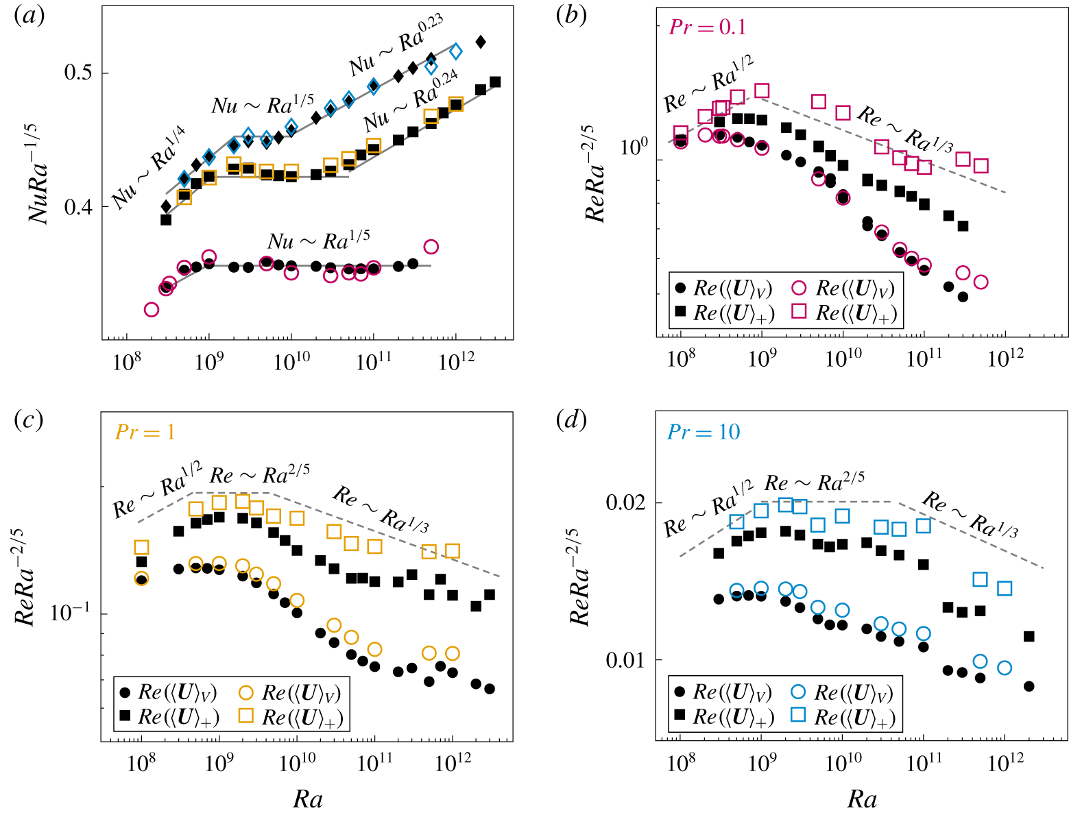
Figure 2. (a) The log–log plot of  $Nu$ versus $Ra$ for $Pr=0.1$ (circles), $Pr=1$ (squares) and $Pr=10$ (diamonds) for CHC (closed symbols) and SHC (open symbols). (b–d) Plots of $Re$ based on $\langle \boldsymbol{U}^{2}\rangle _{V}$ (circles) and of $Re_{+}$ based on $\langle \boldsymbol{U}^{2}\rangle _{+}$ (squares), the kinetic energy average only above the heated plate. The first onsets in the scalings coincide with the instability onsets found in § 3.2; other irregularities correspond to changes in the flow regimes – e.g. (c) $Ra\approx 10^{11}$ and onset to plume regime – as shown in figure 4. The straight scaling lines are a guide to the eye.
The DNS reveal a rather complex scaling dependence, with multiple transitions. Starting from left to right in figure 2(a) we find the following. First,  $Nu\sim Ra^{1/4}$ for lower $Ra$, which corresponds to regime $\text{I}_{l}^{\ast }$ in the Reference Shishkina, Grossmann and LohseSGL model, previously supported by Shishkina & Wagner (Reference Shishkina and Wagner2016) and Ramme & Hansen (Reference Ramme and Hansen2019). As $Ra$ increases, all three sets of data for different $Pr$ show a rather sharp transition to a scaling $Nu\sim Ra^{1/5}$. Note that the critical $Ra$, where this transition occurs, increases with increasing $Pr$. The ${\sim}Ra^{1/5}$ scaling seems to persist up to our highest $Ra$ for $Pr=0.1$. Regime $\text{II}_{l}$ of the Reference Shishkina, Grossmann and LohseSGL model was not observed in our DNS, because $Pr=0.1$ is still too large for this regime (Passaggia, Scotti & White Reference Passaggia, Scotti and White2018). For $Pr=1$ and $10$, the curves rise again at higher $Ra$, leading to a scaling exponent of approximately 0.24 and 0.23. Figure 2(b–d) shows $Re\sim Ra^{2/5}$ for small $Ra$ (regime $\text{I}_{l}$) and $Re\sim Ra^{1/3}$ for larger $Ra$ and no $\text{I}_{l}^{\ast }$ regime at low $Pr$. However, when $Re$ is based on $\langle \boldsymbol{U}^{2}\rangle _{+}$, where $\langle \cdot \rangle _{+}$ denotes average in time and over the volume exclusively above the heated plate(s), we find scaling transitions consistent with the $Nu{-}Ra$ transitions of figure 2(a). In general, the $Re$ scaling is sensitive to its spatial averaging domain. This displays the inhomogeneous nature of HC flows. To explain the scaling transitions, we will have a further closer look at the flow topology and its changes and relate them to the transitions in the scaling relations.
3.2 Dynamics: plumes and oscillations
In general, the HC dynamics are rich in flow structures and instability transitions. Paparella & Young (Reference Paparella and Young2002) observed that HC flows become unsteady with growing  $Ra$, while higher- $Pr$ flows are stable over a broader range of $Ra$. Chiu-Webster, Hinch & Lister (Reference Chiu-Webster, Hinch and Lister2008) and Ramme & Hansen (Reference Ramme and Hansen2019) noticed the existence of time-dependent flows for highly viscous flows. Gayen et al. (Reference Gayen, Griffiths and Hughes2014) showed, for $Pr=5$ and varying $Ra$, that the flow goes through a sequence of stability transitions, starting with the growth of plumes in the BL, followed by convective rolls at higher $Ra$, and finally show fully 3-D turbulence within a region above the hot BL at $Ra\approx 5\times 10^{11}$. The linear stability analysis of Passaggia, Scotti & White (Reference Passaggia, Scotti and White2017) for $Pr=1$ supports these findings and suggests that there exists a competition between 3-D rolls around a streamwise axis and two-dimensional (2-D) Rayleigh–Taylor (RT) instability. The former seem to be dominant in wider cells, as found by Sukhanovsky et al. (Reference Sukhanovsky, Frick, Teymurazov and Batalov2012), whereas the latter seems to be most relevant for no-slip BC in narrow cells. Sheard & King (Reference Sheard and King2011) found that the onset to unsteady flows is independent of vertical confinement for $0.16\leqslant \unicode[STIX]{x1D6E4}\leqslant 2$, and Passaggia et al. (Reference Passaggia, Scotti and White2018) observed the maximum growth for the 2-D plume instabilities at $\unicode[STIX]{x1D6E4}=6$. HC instability was studied also for the cases of a BL synthetic jet (Leigh, Tsai & Sheard Reference Leigh, Tsai and Sheard2016), 2-D HC (Tsai et al. Reference Tsai, Hussam, Fouras and Sheard2016) and different temperature BCs (Tsai et al. Reference Tsai, Hussam, King and Sheard2020).
In our DNS we found the existence of 2-D RT instabilities, which manifest themselves as sheared plumes that arise above the heated plate and which travel towards the endwall (CHC) or the centre (SHC), as shown in figure 3(a). However, for small  $Pr$ and especially in SHC flows, we found a different time-dependent behaviour prior to plumes emerging, which is an oscillatory instability, that breaks symmetry in SHC (3b). These plume- and oscillatory-induced transitions to the unsteady state are explained below.
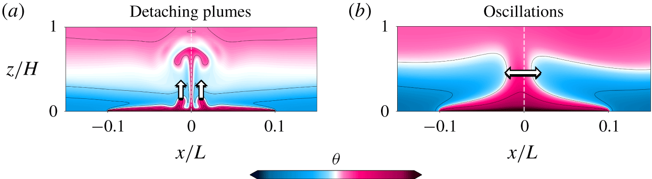
Figure 3. Snapshots of the temperature field for (a) detaching plumes ( $Pr=10$, $Ra=10^{10}$) and (b) oscillations ( $Pr=0.1$, $Ra=3\times 10^{8}$) in SHC.
3.2.1 Plumes
In terms of time scales, detached plumes can occur if the time scale of the development of RT instabilities  $T_{RT}$ is shorter than the advection time scale $T_{wind}$ of the large-scale wind: $T_{RT}/T_{wind}<C_{p}$, for a certain constant $C_{p}$. The $e$-folding time scale of RT instabilities (a characteristic time scale for RT instabilities to grow by the factor $1/e$) equals $T_{RT}\sim \unicode[STIX]{x1D708}^{1/3}/(\unicode[STIX]{x1D6FC}g\unicode[STIX]{x1D6E5})^{2/3}$ (Chandrasekhar Reference Chandrasekhar1981) and the time scale of the wind velocity equals $T_{wind}\sim L^{2}/(Re\,\unicode[STIX]{x1D708})$, which leads to an estimate
 $$\begin{eqnarray}\displaystyle T_{wind}/T_{RT}=Ra^{2/3}/(Re\,Pr^{2/3}). & & \displaystyle\end{eqnarray}$$
 As the plumes detaching regime is anticipated for large  $Pr$, we make use of the scaling relation $Re\sim Pr^{-1}Ra^{1/2}$ of the regime $\text{I}_{l}^{\ast }$ (see table 1), which gives $T_{wind}/T_{RT}\sim Pr^{1/3}Ra^{1/6}$. Thus, a certain critical value of $Pr^{1/3}Ra^{1/6}$, or an equivalent critical value of $Pr^{2}Ra$, determines the onset of the detached plumes. Note that the absolute value of the constant $C_{p}$ can be determined from simulations or experimental data. This relation shows that, for low $Pr$, the critical $Ra$ increases. Physically explained, the larger wind speed of low- $Pr$ flows advects growing plumes faster to the endwall (CHC) or the centre (SHC) before they become distinguishable from the thermal BL.
The solid red curves for  $Pr^{2}Ra\approx 10^{11}$ in figure 4(a) and 4(b) give a rough estimate of the $Pr$ and $Ra$ dependence of the onset of the plume-dominated regime. However, using $Re$ scaling relations from the DNS instead of the Reference Shishkina, Grossmann and LohseSGL model, namely $Re\sim Ra^{2/5}$ (figure 2b) and $Re\sim Pr^{-1}$ (Shishkina & Wagner Reference Shishkina and Wagner2016), together with (3.1), we obtain ${\sim}Pr^{5/4}Ra$. And, indeed, DNS (dashed curves in figure 4) supports that a constant $Pr^{5/4}Ra\approx 9\times 10^{10}$ determines the onset of the detached plumes regime.
At higher  $Ra$, plumes will detach faster, and for sufficiently large $Ra$ one finds multiple plumes detaching from the thermal BL. This phenomenon was reported in Passaggia et al. (Reference Passaggia, Scotti and White2017) for $Ra=9\times 10^{14}$, where plumes were visible immediately after entering the convectively unstable region.

Figure 4. The  $Ra$–
$Ra$– $Pr$ phase space of the flow dynamics: steady (diamonds), oscillations (open squares), plumes (triangles) and chaotic (open circles). The solid lines in (a) and (b) show the theoretically predicted onsets of oscillation and plume regime, the red dashed line the semi-empirical predicted plume regime onset. The other four plots (c–f) show the evolution of the heat flux that enters the left half (red) and the heat flux that enters through the right half of the heated plate (grey), which in the oscillatory regime are in antiphase (represented by dashed lines in (d) and (e)). The normalized frequencies for plume detaching $f_{p}$ and oscillatory movement $f_{o}$ are (c) $f_{p}\approx 0.298$, (d) $f_{p}\approx 0.522$ and $f_{o}\approx 0.070$, (e) $f_{o}\approx 0.068$ and (f) chaotic.
3.2.2 Oscillations
A laminar flow in SHC can be thought of as a configuration of two convective flows in subcells meeting in the centre and circulating in opposite directions. While talking about oscillations, we refer to a horizontal movement of these two large structures and analyse an oscillatory movement at the location where the two rolls meet. This location oscillates periodically around the geometric centre of the cell and thus breaks its symmetry.
Following the same strategy as in the previous section, the onset of oscillations can be described in a simplified way as follows. Assume there exists a temperature fluctuation in one of the subcells near the centreline, which, due to buoyancy forces, leads to a local velocity change  $\unicode[STIX]{x0394}v$ of a flow parcel travelling upwards (relative to the base flow) against the viscous forces. As the speed increases, the pressure drops according to Bernoulli’s theorem, which consequently initiates a horizontal pressure gradient between the two convective subcells. This essentially reflects the underlying role of the pressure term in the Navier–Stokes equations, which can transfer energy between modes of different directions (Batchelor Reference Batchelor1953). Therefore, a vertically directed force (buoyancy) can induce horizontal oscillations.
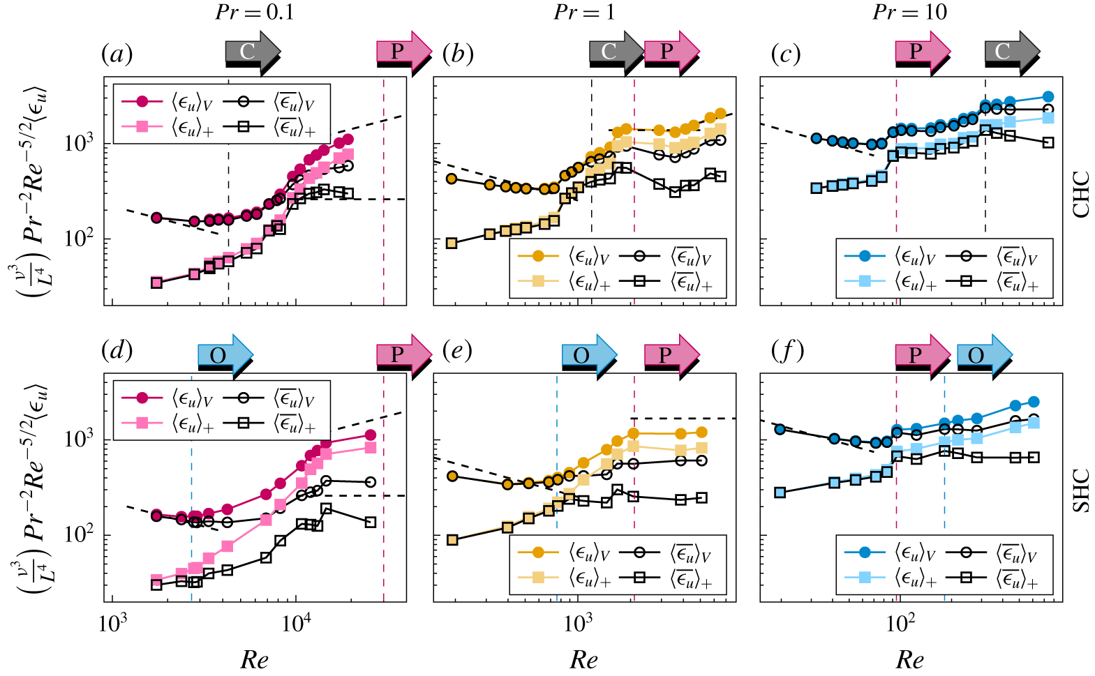
Figure 5. Kinetic dissipation rate versus  $Re$ (as defined in § 3), for (a,d) $Pr=0.1$, (b,e) $Pr=1$ and (c,f) $Pr=10$ in (a–c) CHC and (d–f) SHC. Vertical dashed lines indicate the corresponding onsets of oscillations (O) and plumes (P). Shown are total dissipation rate ( $\unicode[STIX]{x1D716}_{u}$) and contributions from the mean flow ( $\overline{\unicode[STIX]{x1D716}_{u}}$) averaged over the whole domain $\langle \cdot \rangle _{V}$ or averaged specifically over the domain above the heated plate $\langle \cdot \rangle _{+}$. Negative slopes (inclined dashed lines) show $\unicode[STIX]{x1D716}_{u}\sim Re^{2}$; positive slopes show $\unicode[STIX]{x1D716}_{u}\sim Re^{3}$.
The characteristic velocity of this Stokes-type flow is  $\unicode[STIX]{x0394}v\sim (\unicode[STIX]{x1D6FC}g\unicode[STIX]{x0394}L^{2})/\unicode[STIX]{x1D708}$ and the time scale is $T_{p}\approx L/(\unicode[STIX]{x0394}v)=\unicode[STIX]{x1D708}/(\unicode[STIX]{x1D6FC}g\unicode[STIX]{x0394}L)$. The stabilizing antagonist here is the viscous force, which acts as preserving for the symmetric flow profiles and the viscous time scale is $T_{\unicode[STIX]{x1D708}}=L^{2}/\unicode[STIX]{x1D708}$. The oscillations happen as soon as the shear time scale becomes large, unable to smooth out the asymmetric flow profiles at a certain constant value of $T_{\unicode[STIX]{x1D708}}/T_{p}$:
 $$\begin{eqnarray}T_{\unicode[STIX]{x1D708}}/T_{p}=Ra/Pr=Gr.\end{eqnarray}$$
 Our DNS results (figure 4a,b) indicate that the critical value is  $Ra/Pr\approx 5\times 10^{9}$, supporting the above described physical picture. This is consistent with the results of Paparella & Young (Reference Paparella and Young2002), who found that the transition to a time-dependent flow occurs at $Ra/Pr\approx 1.6\times 10^{8}$. The discrepancy in the prefactors is explained by different BCs and that their simulations were 2-D. Two remarks about figure 4 should be made. First, especially for low $Pr$, periodic oscillations exist only near the onset of the instability (figure 4e). With increasing $Ra$, the flow becomes chaotic (figure 4f). Second, we cannot identify the regime of oscillations in CHC, but found the onset to a time-dependent and not plume-determined flow with a similar trend.

Figure 6. Thermal dissipation rate versus  $Re$ (as defined in § 3) for (a,d) $Pr=0.1$, (b,e) $Pr=1$ and (c,f) $Pr=10$ in (a–c) CHC and (d–f) SHC. Vertical dashed lines indicate the corresponding onsets of oscillations (O) and plumes (P). Shown are total dissipation rate ( $\unicode[STIX]{x1D716}_{\unicode[STIX]{x1D703}}$) and contributions from the mean flow ( $\overline{\unicode[STIX]{x1D716}_{\unicode[STIX]{x1D703}}}$) averaged over the whole domain $\langle \cdot \rangle _{V}$ or averaged specifically over the domain above the heated plate $\langle \cdot \rangle _{+}$.
The different plots in figure 4(c–f) show the time signals of the vertical heat flux, averaged over the heated plates. As discussed, low- $Pr$ flows show oscillations and chaotic behaviour, while for large $Pr$ we find the presence of plumes and a combination of plumes and oscillations. In general, the frequency of detaching plumes is an order of magnitude larger than the oscillatory frequency (see caption of figure 4). It remains to be noted that the locations of onsets to time-dependent flows shown in figure 4(a,b) coincide with $Nu$ and $Re$ transitions as seen in figure 2(a,b).
3.3 Dissipation rates
To study how the transition to a time-dependent flow can affect the global scalings (analysed in § 3.1), we now analyse the kinetic ( $\unicode[STIX]{x1D716}_{u}$) and thermal ( $\unicode[STIX]{x1D716}_{\unicode[STIX]{x1D703}}$) dissipation rates and assess the results in the context of the Reference Shishkina, Grossmann and LohseSGL model. Following Ng et al. (Reference Ng, Ooi, Lohse and Chung2015), we decompose the dissipation rates into their mean and fluctuating parts: $\langle \unicode[STIX]{x1D716}_{u}\rangle _{V}=\langle \overline{\unicode[STIX]{x1D716}_{u}}\rangle _{V}+\langle \unicode[STIX]{x1D716}_{u}^{\prime }\rangle _{V}=\unicode[STIX]{x1D708}[\langle (\unicode[STIX]{x2202}U_{i}/\unicode[STIX]{x2202}x_{j})^{2}\rangle _{V}+\langle (\unicode[STIX]{x2202}u_{i}^{\prime }/\unicode[STIX]{x2202}x_{j})^{2}\rangle _{V}]$. This will give us a qualitative understanding about the role that fluctuations have on the mixing process. Additionally, we consider the volume averages restricted to the domain part above the heated plate, $\langle \cdot \rangle _{+}$, where we expect the most turbulent fluctuations.
For  $\langle \unicode[STIX]{x1D716}_{u}\rangle _{V}$ one can expect either the BL scalings ${\sim}Re^{2}$, ${\sim}Re^{5/2}$ or bulk scaling ${\sim}Re^{3}$. Figure 5 shows a non-monotonic behaviour in all cases. First, for the lowest $Re$, the scaling shows approximately $\langle \unicode[STIX]{x1D716}_{u}\rangle _{V}\sim Re^{2}$ behaviour, which corresponds to regime $\text{I}_{l}^{\ast }$ with $Nu\sim Ra^{1/4}$. As $Re$ increases, we observe a rather rapid increase of $\langle \unicode[STIX]{x1D716}_{u}\rangle _{V}$ leading to positive slopes in the compensated plot. The sudden increase in $\langle \unicode[STIX]{x1D716}_{u}\rangle _{V}$ is accompanied by a region where the dissipation of the mean flow starts to drop. The total kinetic dissipation rate in the region above the heated plate $\langle \unicode[STIX]{x1D716}_{u}\rangle _{+}$ increases even stronger and, for high $Ra$, most of the energy dissipates inside this region. The value of $Re$ where the first dissipation increase occurs correlates strongly with the transition to a time-dependent flow, as indicated by the vertical dashed lines. Subsequently, the curves drop again to slopes in between ${\sim}Re^{5/2}$ and ${\sim}Re^{3}$. For high $Re$ and especially for low $Pr$, we observe that the contribution from the mean flow $\langle \overline{\unicode[STIX]{x1D716}_{u}}\rangle _{V}$ is no longer dominant, which matches the observations of Mullarney et al. (Reference Mullarney, Griffiths and Hughes2004) and Scotti & White (Reference Scotti and White2011) that turbulent fluctuations start to become dominating in HC. For our highest $Ra$ and $Pr=1$ (figure 5b), a transition to a turbulent regime ${\sim}Re^{3}$ appears, but more data points at higher $Re$ are needed to extend this trend. Another observation one can make from figure 5(a,d) is that, for increasing $Re$,
$Re$,  $\langle \unicode[STIX]{x1D716}_{u}\rangle _{V}$ and $\langle \unicode[STIX]{x1D716}_{u}\rangle _{+}$ first converge and then slightly diverge again. This is explained by the fact that the region where a turbulent flow is present starts above the heated plate, but then spreads over an increasingly larger volume of the domain.
In figure 6 the thermal dissipation rate is analysed in a similar way. Other than for the kinetic dissipation, there is no observable effect from the onset of the instabilities. Moreover, it is evident that the contributions of turbulent fluctuations is small for all studied  $Ra$ and that the total thermal dissipation is well described by its mean field contribution. Only for our largest $Ra$ and only above the heated plate does the mean flow dissipation deviate slightly from the total thermal dissipation. The scaling is approximately $\unicode[STIX]{x1D716}_{\unicode[STIX]{x1D703}}\sim Re^{1/2}$ to $\unicode[STIX]{x1D716}_{\unicode[STIX]{x1D703}}\sim Re^{3/4}$ and nearly constant.
In summary, we found a strong enhancement of  $\unicode[STIX]{x1D716}_{u}$ in the vicinity of the onset of the first instabilities. These locally occurring changes can cause the sharp scaling transitions, as observed in § 3.1, suggesting not a ‘scale-free’ region. The contributions of the mean dissipation $\overline{\unicode[STIX]{x1D716}_{u}}$ gradually decrease, and for large $Re$ we observe $\unicode[STIX]{x1D716}_{u}\sim Re^{3}$, which hints towards a transition to a turbulent regime. The temperature fluctuations, for all studied $Ra$, contribute little to the total thermal dissipation rate, in contrast to the situation of the kinetic dissipation.
4 Conclusions
Long-runtime DNS were conducted for several decades of  $Ra$ and $Pr=0.1$, 1 and 10, for classical and symmetrical HC, in order to investigate the global scaling relations and the flow dynamics. The obtained results can be summarized as follows.
First, for the same parameters ( $Ra,Pr$), the SHC and CHC systems provide nearly the same heat and momentum transport ( $Nu,Re$). Thus, we conclude that SHC set-ups can serve as a good alternative to CHC in studying HC systems, which may give a better experimental accuracy, since it gets along without isolating the critical hot wall. The $Nu$ versus $Ra$ scaling analysis for both set-ups showed evidence for regimes $\text{I}_{l}$ and $\text{I}_{l}^{\ast }$, according to Shishkina et al. (Reference Shishkina, Grossmann and Lohse2016), as found previously in Shishkina & Wagner (Reference Shishkina and Wagner2016) and Ramme & Hansen (Reference Ramme and Hansen2019). Further, the $Nu$ evolution suggests another transition phase for $Ra>10^{10}$ and $Pr\geqslant 1$, which we found to be presumably related to the transition from a steady to a time-dependent bulk flow. For our highest $Ra=3\times 10^{12}$, both $Pr$ show a slope of $Nu\sim Ra^{0.24}$.
Second, the analysis of the dynamics of HC systems reveals three different unsteady flow regimes: detached plume regime, oscillatory regime in SHC and chaotic regime. The onsets of the former two instabilities have been obtained theoretically up to a constant and were confirmed by our DNS data. Detaching plumes dominate high- $Pr$ flows and are found above a critical $Ra\,Pr^{5/4}\approx 9\times 10^{10}$, while the oscillatory instability starts at a $Ra/Pr\approx 5\times 10^{9}$ and is therefore dominating especially in small- $Pr$ fluids. A subsequent examination of the kinetic and thermal dissipation rates showed that the onsets of these instabilities coincide with a strong increase in the total kinetic dissipation and a simultaneous decrease in its mean field contribution. Our DNS show also that velocity fluctuations become the dominating part of $\langle \unicode[STIX]{x1D716}_{u}\rangle _{V}$, while the temperature fluctuations contribute only a little to $\langle \unicode[STIX]{x1D716}_{\unicode[STIX]{x1D703}}\rangle _{V}$ (less than 5 %).
Further experimental or numerical investigations for  $Ra>10^{12}$ are absolutely crucial for verifying of the other regimes of the Reference Shishkina, Grossmann and LohseSGL model and for the understanding of the role of buoyancy forcing on the ocean dynamics.
Acknowledgements
We acknowledge support by the Deutsche Forschungsgemeinschaft (DFG) under the grant Sh405/10 and the Leibniz Supercomputing Centre (LRZ).
Declaration of interests
The authors report no conflict of interest.
Supplementary material
Supplementary material is available at https://doi.org/10.1017/jfm.2020.211.


 Open access