4.1 Reynolds stress

The fraction of the total Reynolds stress carried by Qs in HST is listed in the first column of table 4. The next two columns give the distribution into Q classes, which roughly agrees with Pumir (Reference Pumir1996). At least within our range of Reynolds numbers, there is a weak trend towards a smaller overall fraction of Reynolds stress being carried by intense Qs as the Reynolds number increases, due both to stronger counter-gradient Q $^{+}$ s and to weaker co-gradient Q $^{-}$ s. Since the fluctuation intensities reflect the sum of Q $^{+}$ s and Q $^{-}$ s, while the Reynolds stress reflects their difference, a consequence is that the correlation coefficient $c_{uv}=-\langle uv\rangle /u^{\prime }v^{\prime }$ between $u$ and $v$ decreases from roughly 0.41 in L38 to 0.37 in H32. A similar trend of $c_{uv}$ is found in wall-bounded flows as the Reynolds number increases. In that case, it is usually attributed to the increased importance of the inactive motions due to the blocking effect of the wall (Townsend Reference Townsend1961), but the present results suggest that there is at least some contribution from an increased cancellation among stress-carrying eddies of different kinds. Table 4 includes data from the ‘logarithmic’ range of wall distances in channel C950. They are comparable to those in HST, including the amount of momentum backscatter (Q $^{+}$ ).

Table 4. Fraction of the Reynolds stress and enstrophy contained in structures with the nominal threshold. The column Q is the percentage of the total Reynolds stress in Qs. The columns Q $^{\pm }$ refer to the stress in each Q class, while the subscript ‘ $C$ ’ refers to Qs whose box diagonal is $d>L_{c}$ , where $L_{c}$ is the Corrsin scale. The final column is the percentage of total enstrophy within vortex clusters. Data for the channel C950 in the range $y^{+}\geqslant 100$ and $y/h<0.4$ are included for comparison (LFJ12). The ‘ $C$ ’ subscript refers in this case to attached Qs.

An important property of channels is that only large attached Q $^{-}$ s carry net Reynolds stress, and that there are basically no large attached Q $^{+}$ s (LFJ12). For smaller detached structures, the counter-gradient contribution of the Q $^{+}$ s cancels the co-gradient contribution of the Q $^{-}$ s. The simplest interpretation is that a net Reynolds stress can only be produced by eddies larger than the Corrsin (Reference Corrsin1958) scale, in which statistical isotropy is broken by coupling with the shear, and that those eddies are mostly co-gradient. Observations in channels cannot easily distinguish whether the asymmetry between Q $^{+}$ and Q $^{-}$ is due to the size of the eddies or to the presence of the wall.

This is tested for HST in the right-hand part of table 4, which lists the fraction of the total stress carried by ‘active’ Q $_{C}$ with $d>L_{c}$ . Comparing with the left-most columns of the table, it is clear that large structures are also responsible for most of the momentum transfer in the absence of walls. In fact, it can be shown that there are very few Q $^{+}$ s larger than $d\approx 5L_{c}$ (see also figure 5 b below). Although not strictly equivalent, Pumir (Reference Pumir1996) mentions that 60 %–70 % of the Reynolds stress in a cubic HST box is carried by the first spanwise mode, whose wavelength is approximately  $10L_{c}$ .

The last column of table 4 shows that the fraction of enstrophy carried by vortex clusters increases slowly with the Reynolds number.

4.2 Flow anisotropy

Figure 4. (a) Shifted Lumley invariants of the Reynolds-stress anisotropy tensor: ▫, M32; ○, H32; ▵, channel C2000 above the buffer layer, with the symbol marking the lower limit, $y^{+}=100$ . Lines with closed symbols are unconditional statistics. Those with open symbols are conditioned to Q $^{-}$ s. For the two HST cases, the identification threshold increases in the direction of the arrow from $H=0.25$ to 4. The channel is only drawn for $H=1.75$ . The inset is a zoom of the region around the nominal threshold $H=1.75$ , marked by symbols. The thin dashed line at the top of the figure is the realisability limit for the invariants. The thicker dashed line that follows the thresholded HST cases is the result for a thresholded velocity field with joint-Gaussian statistics and a correlation coefficient $c_{uv}=-0.4$ . (b) The thin solid elliptical contours are the joint p.d.f., $p_{G}(u/u^{\prime },v/v^{\prime })$ , of two Gaussian variables with $c_{uv}=-0.4$ . They contain 10 %, 50 % and 90 % of the points. The thicker solid ones are $-p_{G}uv/u^{\prime }v^{\prime }$ , with contours $[0.2,0.5,0.8]$ of its maximum. The dashed ones are the same quantity for M32, and the chain-dotted ones are for C2000 at roughly the same Reynolds number $(y/h=0.15)$ . The two hyperbolas are $H=-1.75$ .

Another question is whether the flow within Qs is different from the flow as a whole. Figure 4(a) displays the Lumley invariants, which are defined from the anisotropy tensor of the Reynolds stresses, $\unicode[STIX]{x1D623}_{ij}=\langle u_{i}u_{j}\rangle /\langle u_{i}u_{i}\rangle -\unicode[STIX]{x1D6FF}_{ij}/3$ , as $\unicode[STIX]{x1D701}^{2}=\unicode[STIX]{x1D623}_{ij}\unicode[STIX]{x1D623}_{ji}/6$ and $\unicode[STIX]{x1D709}^{3}=\unicode[STIX]{x1D623}_{ij}\unicode[STIX]{x1D623}_{jk}\unicode[STIX]{x1D623}_{ki}/6$ (Pope Reference Pope2000). The dashed curve at the top of the figure is the two-component realisability limit, and the right-hand vertical axis is the axisymmetric one. The point where the two lines meet in the upper-right part of the plot corresponds to one-component flows. Isotropic flow is at $\unicode[STIX]{x1D709}=\unicode[STIX]{x1D701}=0$ , below the lower-right corner of the plot. The two solid symbols in the lower part of the plot correspond to unconditioned statistics of the HST cases M32 and H32, with the Reynolds number increasing towards the right. The line marked with the solid triangle is C2000 for $y^{+}>100$ , moving towards isotropy as $y$ increases towards the right. The kink in the line is $y/h\approx 0.2$ , and the two points for HST are near the top of the logarithmic layer of the channel, $y/h\approx 0.3{-}0.4$ .

The shorter lines in the upper-right part of the plot are conditioned to points within Q $^{-}$ s. The two roughly diagonal solid curves are the HST cases, with thresholds that increase from $H=0.25$ to $H=4$ in the direction of the arrow. The kinked line marked with a triangle is the channel $(H=1.75)$ , with the kink at $y/h\approx 0.2$ and $y$ increasing away from the triangle $(y^{+}=100)$ . The inset is an enlargement of this part of the plot. The symbols of the HST cases in the inset are for the nominal threshold $H=1.75$ , and show that the conditional statistics in HST also approximate those in the logarithmic layer of channels. It is clear from the figure that Q $^{-}$ s are more dominated by a single velocity component than the flow in general, and that this dominance is higher for the stronger events. Both within and outside the structures, the dominant velocity component is $u$ . A similar figure can be drawn for C950.

However, we should be careful to distinguish between actual properties of the flow and artefacts created by the definition of the Qs. It was shown by Antonia & Atkinson (Reference Antonia and Atkinson1973) and Lu & Willmarth (Reference Lu and Willmarth1973) that the joint p.d.f. of $u$ and $v$ in a boundary layer is essentially that of two Gaussian variables with the correct cross-correlation coefficient, $c_{uv}\approx -0.4$ . The thick dashed line in figure 4(a), largely hidden by the thresholded results, is the locus of the two Lumley invariants of such a joint-Gaussian distribution, thresholded in the same way as the Q $^{-}$ s. It agrees very well with the simulation results.

Figure 4(b) plots the joint p.d.f., $p(u,v)$ , of two Gaussian variables, together with the $H=-1.75$ threshold for Q $^{-}$ s. It also includes the product $p(u,v)uv$ , whose integral is the Reynolds stress, plotted both for the joint-Gaussian distribution and for M32. They agree very well, suggesting that most statistical moments computed for these two velocity components using a joint-Gaussian distribution should agree well with the simulation results. The chain-dotted lines in the figure are for C2000. They also agree reasonably well with the HST and with the Gaussian model, although the asymmetry between Q2s and Q4s suggests that the latter are weaker because they come from the outer part of the channel, where the shear and the velocity fluctuations are weaker.

Figure 5. (a) Anisotropy of the Reynolds-stress tensor within Qs, as a function of their box diagonal: ♢, L38; ▫, M32; ○, H32; $H=1.75$ . Open symbols are for Q $_{uv}$ and closed ones are for Q $_{uw}$ . (b) Probability density function of the box diagonal of Qs defined from different variable pairs. Case M32 and $H=1.75$ : ——, Q $_{uv}$ ; – – –, Q $_{uw}$ ; – ⋅ – ⋅ –, Q $_{vw}$ ; –▵–, Q $_{uv}$ of C2000 centred at $y/h\in (0.1,0.2)$ , where $Re_{\unicode[STIX]{x1D706}}\approx 100$ . In the case of Q $_{uv}$ , open symbols are Q $^{+}$ and closed ones are Q $^{-}$ .

Large and small structures are different from the point of view of the flow anisotropy. The open symbols in figure 5(a) show the mean second Lumley invariant of the flow within Qs, as a function of their size. This quantity is proportional to the Euclidean norm of $\unicode[STIX]{x1D623}_{ij}$ and is a measure of the anisotropy of the Reynolds-stress tensor. It ranges from $\unicode[STIX]{x1D701}=0$ for full isotropy to $\unicode[STIX]{x1D701}=1/3$ for one-component flows. It is clear that the flow is roughly isotropic within structures with $d\lesssim L_{c}$ , which are decoupled from the shear, and only becomes anisotropic within large Qs.

At this point, it may be useful to reflect on the meaning of defining Qs that are much smaller than $L_{c}$ . There is no problem in understanding small vortices, because enstrophy is a scalar quantity, independent of the orientation of the frame of reference. However, Qs are defined in terms of the product of two velocity components, $u$ and $v$ , which can only be defined with reference to a given frame orientation. In a shear flow, the frame of reference is linked to the shear: the streamwise velocity $u$ is the component along the direction of the mean flow, and $v$ is the component in the direction of the shear. Small structures that do not couple with the shear cannot have any statistically preferred direction, and there is no reason for either $u$ or $v$ to be especial. From the point of view of these structures, the mean flow appears as isotropic, and all of the velocity components are equivalent. It was indeed found in LFJ12 that the statistics of small Qs are indistinguishable among many different turbulent flows, including some without local shear, implying that many apparently meaningful statistics of small Qs are artefacts of their definition, and cannot be specific to a particular kind of eddy. For example, the closed symbols in figure 5(a) correspond to Q $_{uw}$ structures, which are defined from points in the flow for which $|uw|>Hu^{\prime }v^{\prime }$ (note that the threshold has been kept as in Q $_{uv}$ , for consistency). For small sizes, the anisotropy within these new structures is essentially the same as within the Q $_{uv}$ . The two types of Qs only differ when they are large, in which case the Q $_{uv}$ couple with the shear, but the Q $_{uw}$ (or Q $_{vw}$ , not shown) do not. It should be noted that the thresholding operation induces some anisotropy even on perfectly isotropic Reynolds-stress tensors, because it tends to select velocity pairs along the diagonal of the quadrant plot (see figure 4 b). It can be shown by direct calculation that a threshold $H=1.75$ results in $\unicode[STIX]{x1D701}\approx 0.1$ for an isotropic joint-Gaussian velocity distribution with $c_{uv}=0$ , and in $\unicode[STIX]{x1D701}\approx 0.25$ for one with $c_{uv}=0.4$ . This is approximately the range of $\unicode[STIX]{x1D701}$ in figure 5(a). Figures 4(a) and 5(a) are consistent with a model of the flow with joint-Gaussian velocity components, in which most of the velocity cross-correlation is contained in large Q $^{-}$ s.

Figure 5(b) further supports the distinction between small and large Qs. It shows the probability distribution of the size of the Qs defined for the three possible combinations of velocity components. They agree almost exactly below $d\approx 5L_{c}$ , and only diverge for structures above that limit. The figure also plots the size distribution for detached Qs in C2000 centred on the band of wall distances that matches the Reynolds number of M32, with similar results. The p.d.f.s of Q $_{uv}$ in HST and channels have been separated into Q $^{+}$ and Q $^{-}$ . Only the latter reach large sizes, presumably because they can grow by drawing energy from the shear. We have already mentioned that there are essentially no large Q $^{+}$ s.

The conclusion from these observations is that Qs much smaller than $L_{c}$ may perhaps be useful for the study of the ‘universal’ inertial range, but they should probably be defined in terms of rotationally invariant properties of the Reynolds-stress tensor. It makes little sense to classify them into quadrants.

Vortex clusters are almost isotropic in terms of the vorticity anisotropy tensor, and essentially identical in this respect to the flow in general. As in channels, vortex clusters in HST tend to be associated with Q $^{-}$ s. In contrast to channels, they are equally distributed between Q2s and Q4s in HST, as required by symmetry. The number fraction of co-gradient vortex clusters, $(uv)_{m}<0$ , is approximately 60 %, almost independent of the Reynolds number and the threshold. However, the fraction of the total cluster volume contained in co-gradient vortex clusters decreases with increasing threshold, from nearly 100 % for $\unicode[STIX]{x1D6FC}\approx 0.1$ to approximately 70 % at the nominal $\unicode[STIX]{x1D6FC}=1.5$ . The fastest decay occurs around the percolation crisis, and is more marked for the higher Reynolds numbers.

Figure 6. Average aspect ratios of the circumscribing boxes for (a) Q $^{-}$  and (b) vortex clusters, as functions of the box diagonal of the structure, scaled with the Corrsin length, for HST and channel C2000, with symbols as in table 1. The channel only includes structures whose minimum distance from the wall is $y^{+}>100$ , and their diagonal is scaled with $L_{c}$ at the centre of gravity of the structures; ——, $a_{xy}$ ; – – –, $a_{zy}$ . (c,d) Average inner and outer dimensions of the structures, as functions of their volume, for HST with symbols as in table 1. Kolmogorov scaling; ——, $r_{3}$ ; – – –, $r_{1}$ . (c) Q $^{-}$ . The two dashed straight lines have slope 1.15 and 0.57 respectively. (d) Vortex clusters. The dashed straight line has slope 1.35.

4.3 Geometry

The shape and orientation of the structures can be characterised by the aspect ratios $a_{ij}=\unicode[STIX]{x1D6E5}_{i}/\unicode[STIX]{x1D6E5}_{j}$ , where the three $\unicode[STIX]{x1D6E5}_{i}$ are the dimensions of the circumscribing parallelepiped. It was found in LFJ12 that the aspect ratios of large wall-attached Q $^{-}$ s are $a_{xy}\approx 3$ and $a_{zy}\approx 1$ , while the smaller detached Qs are roughly isotropic. Figure 6(a) shows the aspect ratios of the Q $^{-}$ s in HST as a function of their box diagonal, scaled with the Corrsin (Reference Corrsin1958) length. The longitudinal aspect ratio $a_{xy}$ increases weakly up to $d\approx 10L_{c}\approx L_{z}$ , which is the scale at which structures begin to feel the effect of the computational box. The spanwise aspect ratio $a_{zy}$ decreases slowly with the size of the structures. The figure also includes data for detached structures in the channel C2000, scaled in the same way. They agree well with HST. In both cases, small structures are roughly isotropic while larger ones tend to become longer (increasing $a_{xy}$ ) and narrower (decreasing $a_{zy}$ ), but there is a range of dimensions of approximately an order of magnitude, $1\lesssim d/L_{c}\lesssim 10$ , in which the aspect ratios remain approximately constant and the Qs can be considered to be geometrically self-similar.

Figure 6(b) shows the same data for vortex clusters. They behave similarly. The vortex clusters in channels tend to be slightly more elongated than the Qs, but it should be remembered that the quantities used to define vortex clusters in HST and channels are not the same.

A more intrinsic indicator of the shape of the structures is provided by the inner and outer dimensions, $r_{1}$ and $r_{3}$ , which are respectively the diameter of their largest inscribed and their smallest circumscribed sphere (here implemented as grid-aligned cubes). Roughly speaking, $r_{3}$ is the diameter of the structure, which typically coincides in our case with $\unicode[STIX]{x1D6E5}_{x}$ , and $r_{1}$ is the thickness of the constituent substructures. These dimensions were used by Catrakis & Dimotakis (Reference Catrakis and Dimotakis1996), Moisy & Jiménez (Reference Moisy and Jiménez2004) and LFJ12 to characterise structures in various turbulent flows. A third dimension can be defined from the volume of the structure as $r_{2}=V/r_{1}r_{3}$ , and can be used to classify simple shapes (Moisy & Jiménez Reference Moisy and Jiménez2004), but its meaning in very irregular shapes is unclear. The two intrinsic dimensions of Q $^{-}$ s and vortex clusters in HST are given in figure 6(c,d) as functions of the structure volume. They follow fairly good power laws, especially for the higher Reynolds numbers. It should be noted that $r_{3}\sim V^{\unicode[STIX]{x1D6FE}/3}$ can be rewritten as $V\sim r_{3}^{3/\unicode[STIX]{x1D6FE}}$ , which can be interpreted as a statistical estimate, $D_{f}=3/\unicode[STIX]{x1D6FE}$ , of the fractal dimension of the set of structures within a given family (LFJ12). Figures 6(c) and 6(d) imply $D_{f}=2.6$ for Q $^{-}$ and $D_{f}=2.2$ for vortex clusters. These are slightly higher than the estimates in LFJ12 for channels (2.3 and 2.0 respectively), but the difference is consistent with the fairly broad distributions that are obtained when estimating the fractal dimensions of individual structures by various methods.

A consequence of figure 6(c,d) is that the bounding box of all of the structures is fairly empty, and becomes emptier for the larger volumes. Thus, if we define a ‘fill fraction’ as $V/r_{3}^{3}$ , it varies from approximately 0.1 for the smallest Qs and vortex clusters to $3\times 10^{-3}$ and $3\times 10^{-4}$ respectively for the largest ones.

The inner dimension of vortex clusters in figure 6(d) is $r_{1}\approx 6\unicode[STIX]{x1D702}$ , independently of the cluster volume, which approximately agrees with the diameter of individual filamentary vortices in turbulence (Jiménez & Wray Reference Jiménez and Wray1998; Tanahashi, Iwase & Miyauchi Reference Tanahashi, Iwase and Miyauchi2001; del Álamo et al. Reference del Álamo, Jiménez, Zandonade and Moser2006; Pirozzoli, Bernardini & Grasso Reference Pirozzoli, Bernardini and Grasso2008; Stanislas, Perret & Foucaut Reference Stanislas, Perret and Foucaut2008). It is also consistent with the description of vortex clusters as ‘sponges of strings’ (LFJ12).

The inner dimension of the Qs in figure 6(c), $r_{1}\sim (\unicode[STIX]{x1D702}r_{3})^{1/2}$ , is more interesting because it depends on the volume, and is therefore a property of the structures rather than of the flow. These structures are described in LFJ12 as ‘sponges of flakes’, mainly from visual observation and from their relatively high fractal dimension. It follows from the definition of $r_{2}$ and from the power laws in figure 6(c) that $r_{2}\sim r_{3}$ in Qs, which also suggests flakes (see figure 3 a). A rough model that at least reproduces the functional dependence of $r_{1}$ can be constructed if we interpret these flakes as viscosity-dominated layers of thickness $r_{1}$ . We know from the definition of Qs that the velocity difference across them is of the order of $u^{\prime }$ , so that we can approximate the resulting structure-dependent mean strain as $s\approx u^{\prime }/r_{3}$ in a coarse-grained sense. Some algebra shows that the corresponding viscous equilibrium thickness is $r_{1}=(\unicode[STIX]{x1D708}/s)^{1/2}\approx (\unicode[STIX]{x1D708}/u^{\prime }\unicode[STIX]{x1D702})^{1/2}(\unicode[STIX]{x1D702}r_{3})^{1/2}$ . The prefactor in this estimate is proportional to $Re_{\unicode[STIX]{x1D706}}^{-1/4}$ , and varies between 0.28 and 0.4 in our DNS. The lower dashed line in figure 6(c) is drawn with a prefactor 0.35 and, given the qualitative nature of the above argument, agrees reasonably well with the measured $r_{1}$ .

It is clear that this argument can only be approximate, particularly regarding the estimation of the driving strain. It follows from well-known integral constraints that the predominant strain in turbulence is of the order of $\unicode[STIX]{x1D714}^{\prime }\sim u^{\prime }/\unicode[STIX]{x1D706}$ , and that the associated viscous length is the Kolmogorov scale $\unicode[STIX]{x1D702}$ (Pope Reference Pope2000). However, Hunt, Eames & Westerweel (Reference Hunt, Eames and Westerweel2006) argued that strong shear layers exclude the small-scale strain, leaving only the strain associated with the depth of the layer. In our case, the thresholding operation used to define the structures guarantees that they represent relatively strong velocity gradients, but we will see in § 5 that Qs only have velocity differences of order $u^{\prime }$ across their largest dimension, if at all, justifying our strain estimate in the previous paragraph. Smaller corrugations, such as those of size $O(r_{1})$ , correspond to weaker local velocity fluctuations that happen to cross the sharp threshold used in the identification. In the limit of very large structures, with $r_{3}\sim L_{\unicode[STIX]{x1D700}}$ , the previous estimate becomes $r_{1}\sim \unicode[STIX]{x1D706}$ , and the argument reduces to the one in Hunt et al. (Reference Hunt, Eames and Westerweel2006), but the present results require extension of the analysis to the full range of scales.

Figure 7. (a) Probability density function of the aspect ratio $a_{xy}$ of Q $^{-}$ s in C2000 as a function of their minimum distance from the wall. Each vertical section is the individual p.d.f. at one wall distance. Contours contain 50 % and 95 % of the data; –▵–, Average aspect ratio. The vertical dashed line is $y_{min}^{+}=20$ . Symbols are the mean and standard deviation of $a_{xy}$ in HST, as in table 1. They are plotted at arbitrary $y$ locations. (b) As in (a), for $a_{zy}$ . (c) Sketch of the root and body of a large attached Q2. Flow is from left to right, and the Q2 is qualitatively coloured with the distance from the wall. (d) Average $a_{xz}$ of Q $^{-}$ s with $y_{min}^{+}<100$ in C2000, as a function of their vertical dimension. See the sketch in (c) for definitions; ——, $\unicode[STIX]{x1D6E5}_{x}/\unicode[STIX]{x1D6E5}_{z}$ ; – – –, $\unicode[STIX]{x1D6E5}_{x,100}/\unicode[STIX]{x1D6E5}_{z}$ ; - - - -, $(\unicode[STIX]{x1D6E5}_{x}-\unicode[STIX]{x1D6E5}_{x,100})^{+}=100$ ; – ⋅ – ⋅ –, $\unicode[STIX]{x1D6E5}_{x,100}/\unicode[STIX]{x1D6E5}_{z}$ for Q $^{-}$ s constructed from points above $y^{+}=100$ . The short horizontal dashed line is $a_{xz}=1.27$ , as in the detached and HST structures.

4.4 Attached versus detached eddies in channels

Up to now, we have compared the structures in HST with the detached eddies in channels. Most large eddies in channels are attached, because the wall limits how high they can grow but not their wall-parallel dimensions (Townsend Reference Townsend1961). Attached and detached eddies behave differently, particularly in their geometry. It was shown in LFJ12 that attached Q $^{-}$ s in channels have $a_{xy}\approx 3$ , while we have seen that those in HST have $a_{xy}\approx 1.2$ . The higher elongations of the largest channel eddies in figures 6(a) and 6(b) correspond to attached structures.

The origin of this higher elongation is explored in figure 7(a), which contains the p.d.f. of $a_{xy}$ in C2000 as a function of the minimum distance of the structures from the wall. This is the distance originally used in AJZM06 to differentiate between attached and detached objects. The figure shows that only strictly attached structures $(y_{min}^{+}\lesssim 20)$ are elongated. Those farther from the wall have elongations very similar to those in HST. Interestingly, figure 7(b) shows that $a_{zy}$ is similar for attached and detached Qs, in agreement with the observation by Lozano-Durán & Jiménez (Reference Lozano-Durán and Jiménez2014) that large attached Qs grow predominantly by merging with other eddies in front and behind, but not sideways.

The relatively good scaling of figures 6(a) and 6(b) with $L_{c}$ suggests that the elongation of the structures is a consequence of their interaction with the mean shear. It was shown by Corrsin (Reference Corrsin1958) that the relevant parameter is $S^{\ast }=Sq^{2}/\unicode[STIX]{x1D700}$ , which measures the ratio between the eddy turnover and the shear deformation time. When $S^{\ast }\gg 1$ , the structures are controlled by the shear, but for lower $S^{\ast }$ , nonlinear effects isotropise them. Jiménez (Reference Jiménez2013b ) showed that $S^{\ast }$ is everywhere moderate in channels except for $y^{+}\lesssim 25$ , where it grows to $S^{\ast }\approx 40$ . The origin of the large elongation of attached Qs in channels could thus be the high $S^{\ast }$ in the viscous layer. In fact, it was shown by Lozano-Durán & Jiménez (Reference Lozano-Durán and Jiménez2014) that large attached Qs have two components with different properties: a coherent one above $y^{+}\approx 100$ which approximately advects with the local mean velocity and a more elongated ‘root’ near the wall whose small-scale features move at a different velocity from the structure itself, and which is constantly being shredded by the shear and recreated by viscosity (see the sketch in figure 7 c). However, it is difficult to distinguish between the averaged properties of the flow within attached and detached eddies, both of which can be described by the joint-Gaussian model discussed in figure 4. Even if the buffer layer behaves differently from the rest of the flow, it constitutes too small a part of the large attached eddies to influence their statistics.

Whether the near-wall region, as opposed to the viscous sublayer, is responsible for the higher elongation of the attached Q $^{-}$ s is tested in figure 7(d), which compares $a_{xz}$ for the attached eddies as functions of the overall eddy height, computed in three different ways. The solid line represents all of the large attached Q $^{-}$ s, defined for this particular figure as those with $y_{min}^{+}<100$ . The triangles are the dimensions of the part of those same attached eddies that extends above $y^{+}=100$ . They therefore subtract the effect of the near-wall region (figure 7 c), and show that relatively small attached eddies owe the higher elongation to the root. Their upper coherent component has an aspect ratio similar to those of detached eddies, but this effect decreases for larger structures and is negligible for the largest ones. The dashed line in figure 7(d) is a model in which the extra elongation is approximated by a fixed extra length $\unicode[STIX]{x1D6E5}_{x}^{+}=100$ , and fits the data reasonably well. This is the order of magnitude of the size of the minimal buffer-layer flow unit (Jiménez & Moin Reference Jiménez and Moin1991), suggesting that the near-wall root is formed by multiple such units underneath the coherent outer component, some of which accidentally stick in front of or behind it. Visual inspection of individual structures confirms that this is a reasonable description (see, for example, figures 8 and 12 in LFJ12). Since these minimal structures have a fixed size in viscous units, their effect on the large eddies that reach into the logarithmic and outer layers is negligible.

Because of the way in which attached Qs have been defined in the previous paragraph, the points forming the truncated and attached Qs above $y^{+}=100$ are the same, although clustered in different ways. The chain-dotted line in figure 7(d) also refers to the dimensions of eddies measured above $y^{+}=100$ , but for Qs that have been computed using only points above that level. There is no way to know whether some of these truncated Qs are connected below $y^{+}=100$ , and the difference between the chain-dotted line and the triangles measures the importance of those ‘hidden’ near-wall connections. It is clear that the truncated Qs cannot be longer than the full ones, but it is interesting that the shortening increases with the size of the eddy. While the difference in length is $\unicode[STIX]{x1D6E5}_{x}^{+}\approx 0$ for the smallest eddies, it grows to $\unicode[STIX]{x1D6E5}_{x}^{+}\approx 1500$ for the tallest ones at the right end of the figure, which is approximately 20 % of their total length.

The implied model is that large Qs in the channel grow until they hit the wall. Once they do, the outer part of the eddy keeps growing in length and width but not in height, as its bottom is continually truncated by the high shear at the wall and by viscosity. At the same time, the elongation of the attached eddies increases because they tend to get ‘spuriously’ connected near the wall. That the largest attached eddies owe part of their size to spurious connections near the wall was already noted by LFJ12.

In the rest of the paper, we will mostly restrict ourselves to comparisons of HST with detached eddies in channels, particularly with those with $y_{min}^{+}\geqslant 100$ .

5.1 Relative positions of structures of the same kind

Figure 8(a) displays the mean value of the absolute distance, $r^{(ii)}=|\boldsymbol{r}^{(ii)}|$ (no summation), from a Q to its closest Q of the same kind, as a function of the box diagonal of the reference structure. Below $d\approx 50\unicode[STIX]{x1D702}$ , the mean distance is constant, $r^{(44)}\approx 50\unicode[STIX]{x1D702}$ , which is roughly the wavelength of the maximum of the dissipation spectrum in most turbulent flows (Jiménez Reference Jiménez2013b ). This is also the size of the structures in the dissipative end of the turbulence spectrum that were shown by Yoshida, Yamaguchi & Kaneda (Reference Yoshida, Yamaguchi and Kaneda2005) to be enslaved to the larger inertial ones. They are essentially Kolmogorov viscous eddies, and the figure shows that they are densely packed on average, separated by other eddies of similar size. Above $d\approx 50\unicode[STIX]{x1D702}$ , the distance to the closest comparable structure is $r^{(44)}\approx d$ up to the largest available scale, $d\approx L_{\unicode[STIX]{x1D700}}$ . These are the self-similar inertial eddies, and they are also densely packed. It follows from their definition that the velocity fluctuations in Qs are $O(u^{\prime })$ with respect to the mean, but the velocity difference between neighbouring structures need not be of the same order. The close packing of Qs of the same kind suggests that they are pieces of larger structures. The Reynolds stress of the composite structure is $O({u^{\prime }}^{2})$ , as required by the identification procedure, but the isosurface bounding it can become broken into smaller pieces when the Reynolds stress fluctuates slightly above or below the chosen threshold.

Figure 8(b) displays two-dimensional p.d.f.s of the relative position of neighbouring ‘small’ Q4s $(d<4L_{c})$ . In channels, attached Qs are arranged streamwise in the $(x,z)$ plane (LFJ12). This is still true in HST, but, in addition, the p.d.f. is inclined downwards in the streamwise direction. It should be noted that the p.d.f.s included for detached Qs in the channel agree well with HST, and are also inclined downwards. Because of the symmetry of HST, the same inclination is found for Q2s in HST. The downward tilt of the Q2s is slightly less marked in the channels (not shown); apparently, even these relatively small detached Qs are influenced by the wall or by the inhomogeneity of the mean shear. Also not shown is the p.d.f. of the relative position of neighbouring large Q4s $(d\geqslant 4L_{c})$ . It is still true that these eddies are aligned streamwise, but the downwards inclination is less marked than for the small structures, presumably reflecting the anisotropy of the large-scale velocities. As we saw in the discussion of figures 4(a) and 5(a), $u$ is the predominant velocity component, and the flow anisotropy is mainly associated with the largest structures.

A three-dimensional view of $p^{44}(\unicode[STIX]{x1D739})$ is shown in figure 8(c), and confirms that the p.d.f. is concentrated at two diagonal locations in front of and behind the reference Q4. It is tempting to associate its downwards tilt with a systematic vertical meandering of the streaks, but the explanation is probably simpler. We have seen that small eddies are basically decoupled from the shear and the mean velocity. However, Q4s are defined by $u>0$ and $v<0$ , so that the flow velocity within them is tilted downwards, and we have seen in figure 8(a) that their separation suggests that they are pieces of larger structures whose connectivity is broken by weaker velocity fluctuations. It is then natural to expect from continuity that the closest Q of the same kind is located in the direction of the predominant velocity fluctuations which, in the case of Q4s, is the downwards diagonal. This is sketched by the nominal velocity arrows in figure 8(c), and confirmed by figure 8(d), which contains the relative position of Q1s. They are predominantly arranged along the upwards diagonal, corresponding to the mean velocity in a Q1. This is even more clearly shown by the lines with closed squares in figure 8(b,d), which correspond to small Q $_{uw}$ eddies in M32. Their separations agree well with those of the Q $_{uv}$ , and their positions are aligned along their corresponding diagonals, although in the $(x,z)$ plane, rather than in $(x,y)$ .

The interpretation that neighbouring Qs of the same kind are fragments of larger structures is confirmed by the conditional velocity field in figure 8(e), which shows the streamwise velocity conditioned to the presence of a pair of Q4s, in terms of the similarity coordinate,

(5.3) $$\begin{eqnarray}\unicode[STIX]{x1D739}=(\boldsymbol{x}-\boldsymbol{x}_{cog})/d_{12},\end{eqnarray}$$

where $\boldsymbol{x}_{cog}$ is the position of the common centre of gravity of the Qs involved in the pair and $d_{12}=(d_{1}+d_{2})/2$ is the mean of their diagonals $d_{j}$ . The two neighbours are seen to be enclosed within the same velocity structure.

Figure 9. Relative position of the closest Q4 to a given Q2: ▫, M32; ○, H32; ▵, C2000 with $y_{min}^{+}\geqslant 100$ . The solid squares are Q $_{uw}$ in M32. (a) Average closest distance $\langle r^{(24)}\rangle$ , as a function of the diagonal of the reference Q2. The dashed line has slope $2/3$ . (b) Probability density function of $r^{(24)}$ for different size bands centred at $d^{(2)}/\unicode[STIX]{x1D702}=50,100,200,400$ , with the wider tails corresponding to the smaller structures. Case M32. Each p.d.f. is normalised with its mean value. The dashed line is the nearest-neighbour distribution for a Poisson point set in three-dimensional space. (c) Probability of ‘isolated’ Q2s, defined as those with no neighbour closer than $r^{(24)}=2d^{(2)}$ , as a function of the diagonal of the reference Q2. (d) Anisotropy of the position of the closest Q4 with respect to a given Q2, as a function of $d^{(2)}$ .

5.2 Relative positions of structures of different kind

Figure 9(a) displays the mean distance between Qs of different kind (from a reference Q2 to its closest Q4). It contains the same viscous range as in the previous case, $d\lesssim 50\unicode[STIX]{x1D702}$ , but the distance between these Kolmogorov structures scales with the Taylor microscale $r^{(24)}\approx 3\unicode[STIX]{x1D706}$ . In addition, the inertial range is not self-similar any more, with $r^{(24)}\sim d^{(0.5{-}0.7)}$ . Both issues are presumably related and, although they might admit dynamical explanations such as those given in § 4.3 for the intrinsic dimensions of the Qs, the reason is again probably simpler and geometrical. It follows from the distribution of the volume of the Qs given in § 3, $p(V)\sim V^{-5/3}$ , that the probability distribution of $d\sim V^{1/3}$ is $p(d)=p(V)\,(\,\text{d}V/\,\text{d}d)\sim d^{-\unicode[STIX]{x1D6FD}}$ , with $\unicode[STIX]{x1D6FD}=3$ . In practice, the exponent ranges from $\unicode[STIX]{x1D6FD}=2.8$ for L38 to $\unicode[STIX]{x1D6FD}=3.3$ for H32 and $\unicode[STIX]{x1D6FD}=4$ for C2000. When looking for nearest neighbours satisfying condition (5.2), the number of available candidates per unit volume is then proportional to

(5.4) $$\begin{eqnarray}n\sim \int _{d/2}^{2d}\unicode[STIX]{x1D705}^{-\unicode[STIX]{x1D6FD}}\,\text{d}\unicode[STIX]{x1D705}\sim d^{1-\unicode[STIX]{x1D6FD}},\end{eqnarray}$$

where $d$ without a sub- or super-index should be understood as applying to the reference structure in a pair. Because of the restriction (5.2), such $d$ is also proportional to the average diameter of the two structures being considered. Assuming a statistically uniform spatial distribution of the candidate structures, the average distance from a randomly chosen point to the closest structure is $\langle r^{(ij)}\rangle \sim n^{-1/3}\sim d^{(\unicode[STIX]{x1D6FD}-1)/3}$ . The dashed line in figure 9(a) is drawn with slope $2/3\;(\unicode[STIX]{x1D6FD}=3)$ . It represents the data well, although the slope increase from M32 to C2000 (corresponding to an increase in $\unicode[STIX]{x1D6FD}$ ) is clear. In particular, it should be noted that $\unicode[STIX]{x1D6FD}=4$ results in $\langle r\rangle \sim d$ , which agrees with the steeper slope of C2000 in figure 9(a), and with the results in LFJ12. This dependence also explains the scaling of the minimum distance with $\unicode[STIX]{x1D706}$ . Invoking the independence of the large scales of turbulence with respect to the Reynolds number, which requires that structures with $d=O(L_{c})$ should be separated by distances $r=O(L_{c})$ , the previous relation should be written as

(5.5) $$\begin{eqnarray}\langle r^{(ij)}\rangle \sim L_{c}^{(4-\unicode[STIX]{x1D6FD})/3}d^{(\unicode[STIX]{x1D6FD}-1)/3}.\end{eqnarray}$$

Substituting $d\sim O(\unicode[STIX]{x1D702})$ in this equation, we obtain $r\sim O(\unicode[STIX]{x1D706})Re_{\unicode[STIX]{x1D706}}^{(3-\unicode[STIX]{x1D6FD})/2}$ , which is very close to $\unicode[STIX]{x1D706}$ when $\unicode[STIX]{x1D6FD}\approx 3$ .

The rest of figure 9 tests this model. Figure 9(b) displays the p.d.f.s of the distance among Q4s and Q2s for different bands of sizes of the reference structure in the ‘inertial’ range, $50\unicode[STIX]{x1D702}<d^{(2)}<4L_{c}$ , each of them normalised by their mean separation. They are compared with the distribution of closest distances for a Poisson point set in which the average number of points within a sphere of radius $r$ is $N(r)=(r/R)^{3}$ . This distribution can be computed as the derivative with respect to $r$ of the probability of finding no points closer than $r$ (Feller Reference Feller1971),

(5.6) $$\begin{eqnarray}p_{nn}(r)=(\,\text{d}N/\,\text{d}r)\exp (-N)=3r^{2}/R^{3}\exp (-r^{3}/R^{3}).\end{eqnarray}$$

The parameter $R$ is related both to the average point density per unit volume, $n=3/4\unicode[STIX]{x03C0}R^{3}$ , and to the average distance to the nearest neighbour, $\langle r\rangle \approx 0.89R$ . The different p.d.f.s agree reasonably well among themselves and with the Poisson model.

It was found by LFJ12 that tall attached Q2s in channels tend to be associated with similar Q4s within a distance of $O(d)$ , and that such pairs behave like coherent flow units that organise the flow between the pair into a quasi-streamwise ‘roller’. Structures that are much farther apart should be considered as isolated, and are unlikely to influence each other. A consequence of the two previous figures is that the average separation between small Qs of different kind tends to be much larger than their size, so that most of them cannot be considered to form part of a pair. Figure 9(c) shows the probability that a Q2 is isolated in the sense that its closest Q4 is at $r^{(24)}>\unicode[STIX]{x1D6FC}_{d}d^{(2)}$ , with $\unicode[STIX]{x1D6FC}_{d}=2$ . It shows that Qs smaller than $d/\unicode[STIX]{x1D706}\approx 5$ are most likely isolated, but that larger ones are not. The same holds for detached Qs in channels. Several scalings of $d$ were tested for figure 9(c), and the one with $\unicode[STIX]{x1D706}$ works best for this particular choice of $\unicode[STIX]{x1D6FC}_{d}$ . This is not very surprising, because we have seen that the smallest distance between different kinds of Qs is also $O(\unicode[STIX]{x1D706})$ , but it is inconsistent with (5.5), which implies that $r\sim d$ when $r\sim L_{c}$ . Changing the multiple $\unicode[STIX]{x1D6FC}_{d}$ used to define isolated structures moves the curves in figure 9(c) to the right or left, and also changes their scaling slightly. The choice above, $\unicode[STIX]{x1D6FC}_{d}=2$ , was selected for consistency with the scaling in figure 9(d), which is independent of $\unicode[STIX]{x1D6FC}_{d}$ , but we will see later that $\unicode[STIX]{x1D6FC}_{d}=1$ leads to sharper conditional flow fields for pairs of structures.

In fact, most of the rest of this section could be written substituting $\unicode[STIX]{x1D706}^{1/3}$ for $L_{c}^{1/3}$ in (5.5). The available range of Reynolds numbers is not sufficient to distinguish the $Re_{\unicode[STIX]{x1D706}}^{1/3}$ factor between the two scalings, which only changes by $1.3$ among the cases in figure 9. It can be shown that the $r\sim d^{2/3}$ law ceases to hold for $d^{(2)}\gtrsim 5L_{c}$ , above which limit the mean distance is $r/L_{c}=5{-}10$ for all Reynolds numbers. This limit corresponds to $10\unicode[STIX]{x1D706}$ in M32 and $20\unicode[STIX]{x1D706}$ in H32, which are not far from where the structures become paired in figure 9(c). In fact, it can be argued that only H32 has a convincing 2/3 range in figure 9(a). From now on, in the absence of data over a wider range of Reynolds number, we plot each figure in the scaling that works best for it, without paying too much attention to mutual consistency.

Finally, figure 9(d) tests the preferential orientation of the location of Q4s with respect to the reference Q2. The Poisson model suggests that mutually isolated structures should be isotropically distributed with respect to each other, while only those that form pairs would be organised in particular ways (LFJ12). A position-anisotropy tensor can be defined as $\unicode[STIX]{x1D70C}_{ij}=\langle r_{i}r_{j}\rangle /\langle r_{k}r_{k}\rangle -\unicode[STIX]{x1D6FF}_{ij}/3$ , where $\boldsymbol{r}$ is the relative position vector between two structures. The anisotropy of the relative positions can be measured by the second invariant $\unicode[STIX]{x1D701}_{rr}^{2}=\unicode[STIX]{x1D70C}_{ij}\unicode[STIX]{x1D70C}_{ji}/6$ of $\unicode[STIX]{x1D70C}_{ij}$ , defined in the same way as the Lumley invariant of the Reynolds-stress tensor. Although $\unicode[STIX]{x1D701}_{rr}$ is only an incomplete measure of isotropy, figure 9(d) shows that small Qs are essentially isotropically distributed with respect to each other, as required by the Poisson model, but that the isotropy breaks down for sizes of the same order as those at which the structures begin to pair. The behaviour of channels is different in this respect, presumably because of the interference from the wall, and the preferential orientation begins for much smaller eddies that do not necessarily form pairs.

It should be noted that these arguments do not apply to Qs of the same kind, where we have seen that neighbouring structures may be separated by relatively weak fluctuations that happen to cross the detection threshold. Candidate neighbours cannot then be assumed to be uniformly distributed. On the contrary, Qs of different kind are necessarily separated by velocity differences $O(u^{\prime })$ , and, if we restrict the magnitude of the velocity gradients to their average value, $O(\unicode[STIX]{x1D714}^{\prime })$ , such velocity jumps are unlikely to occur across distances much smaller than $\unicode[STIX]{x1D706}\sim u^{\prime }/\unicode[STIX]{x1D714}^{\prime }$ .

Figure 10. Cross-sections of the three-dimensional joint p.d.f. of the position of the closest Q4 relative to a given Q2: ▫, M32; ○, H32; ▵, C2000 with $y_{min}^{+}\geqslant 100$ . The similarity variable is defined in (5.7). The p.d.f.s are integrated over $\unicode[STIX]{x1D707}=\pm 0.2$ normal to the plane of the plot, and symmetrised around $\unicode[STIX]{x1D707}_{z}=0$ . (a) In the $(z,x)$ plane, for small Q4s $(50\unicode[STIX]{x1D702}<d^{(2)}<2L_{c})$ . (b) In the diagonal plane orthogonal to $\boldsymbol{r}=[1,-1,0]$ , for small Q4s. The probability contours in (a,b) contain the highest 30 % of the data. (c) Three-dimensional $p^{24}$ in M32 for $d<4L_{c}$ , as in (b). The black arrow at the centre of the box is the nominal velocity for a Q2. That at the right-hand end of the p.d.f. is a Q4, and opposes the central one, suggesting a mechanism by which the p.d.f. is excluded from the diagonal and concentrated at the equatorial plane. (d) As in (b) for H32: ——, $50\unicode[STIX]{x1D702}<d^{(2)}<L_{c}/2$ ; - - - -, $d^{(2)}>L_{c}$ . Contours contain 20 % and 40 % of the data.

Figure 10 displays sections of the three-dimensional p.d.f.s of the relative positions of Q4s with respect to a Q2. As in figure 8, statistics can only be compiled by scaling distances properly and, following (5.5), the similarity scaling (5.1) is substituted by

(5.7) $$\begin{eqnarray}\unicode[STIX]{x1D741}^{(ij)}=\frac{\boldsymbol{x}^{(j)}-\boldsymbol{x}^{(i)}}{{d^{(i)}}^{2/3}L_{c}^{1/3}}.\end{eqnarray}$$

It should be noted that the same scale is used for all of the flows, even if figure 9(a) shows that their actual average distance is not exactly the same, especially for the channel. Figure 10(a), which displays the section of the p.d.f.s in the $(z,x)$ plane, shows that the three flows collapse well. The result is similar to that found by LFJ12 for attached Qs in channels. There is essentially no probability of finding a Q4 in front of or behind the Q2, and the closest Q4s are found in the spanwise direction. The symmetry of this p.d.f. is statistical. It was shown in LFJ12 that, when the direction of the closest partner is defined as positive, the groups are found to be pairs, not trios; i.e. the second-closest partner is either much farther away, missing or in the same direction as the closest one. The same was found to be true here.

However, the Qs in figure 10(a) are relatively small $(d<2L_{c})$ , and arguments similar to the ones used in the previous section for $\boldsymbol{r}^{(44)}$ suggest that some of the properties of the p.d.f. might be kinematic. Since the perturbation velocity in a Q2 is directed along the downwards streamwise diagonal, $\boldsymbol{u}\sim [-1,1,0]$ , it tends to exclude from that direction structures with an opposing velocity ( $\boldsymbol{u}\sim [1,-1,0]$ for a Q4). In fact, the p.d.f. of $\boldsymbol{r}^{(24)}$ should be complementary to that for $\boldsymbol{r}^{(44)}$ : empty along the downwards sloping diagonal and concentrated on the equatorial plane normal to that direction. This turns out to be true. Figure 10(b) shows a section along this inclined equatorial plane and reveals that the two high-probability regions in figure 10(a) are sections of an inclined arch or semicircle, whose dimensions also collapse well among the different flows. The three-dimensional view in figure 10(c) shows that the fact that this equatorial section is not a full torus is not due to the misalignment of its plane. This figure also sketches the argument above about how conflicting axial velocities restrict where the p.d.f. can be expected to be located in the space of relative positions. Figure 10(d) shows the relative p.d.f.s of small and large Qs, and proves that the arch-like character is predominantly a property of large structures; small ones are distributed more isotropically in the equatorial plane. It should be emphasised again that the symmetry of the distributions in figure 10 is statistical, due to the symmetry S1 in § 4. In fact, this symmetry is explicitly enforced on the plot to improve statistics. It should also be made clear that these distributions do not represent the shape of any structure, even on the average. They describe probabilities of the relative positions of the centres of gravity of different structures of different kind.

The arched p.d.f. in figure 10(c) is different from that between pairs of attached Qs in channels, and also different from the conditional distribution of close pairs of Qs of different kind shown later in § 6. In these two cases, the interaction between the structures in the pair is strong, and the predominant probability distribution is formed by a Q2 and a Q4 located spanwise from one another. The p.d.f.s in figure 10 are dominated by small structures that are typically far from each other, and represent the effect of the larger flow features containing them. The shape of the p.d.f. depends on the structures involved. It follows from symmetry that the arches in figure 10 become ‘Us’ for the position of Q2s relative to a Q4 in HST. The same is true for the detached Qs in channels. The interpretation of these shapes is interesting. The Q4s in figure 10 are structures of high streamwise velocity. The figure shows that they tend to be located above or to the side of the low-streamwise-velocity Q2s, but not below. The complementary shape of the p.d.f. of $\boldsymbol{r}^{(42)}$ carries the same message: high velocity is above low velocity in the presence of a Q $^{-}$ . This is the direction of the ambient shear, and, since the Qs are defined from perturbation velocities, the implication is that they tend to be located in regions in which the shear is higher than the mean. This is reasonable, since they have to draw their energy from the local velocity difference, and has been mentioned often in the context of vortical structures (see, for example, Adrian Reference Adrian2007). These high-shear regions can be interpreted as the sharp interfaces between relatively uniform streamwise-velocity streaks, which are known to be layers of high activity both in the buffer region (Kim, Moin & Moser Reference Kim, Moin and Moser1987; Jiménez & Pinelli Reference Jiménez and Pinelli1999; Schoppa & Hussain Reference Schoppa and Hussain2002) and in the logarithmic layer (Meinhart & Adrian Reference Meinhart and Adrian1995; Flores & Jiménez Reference Flores and Jiménez2006). In the buffer layer, the high shear close to the wall substitutes the horizontal segment of the arch in figure 10, and the attached Qs are only concentrated in the lateral boundaries between low- and high-velocity streaks (although see the enveloping high-velocity streak in figure 12d of LFJ12, and the conditional flow fields in the next section). What figure 10 implies is that, away from the wall or in HST, the Qs concentrate either on the side or on the top boundary of the low-velocity streaks. A little thought shows that it also implies that only the top part of the low-velocity streaks and the bottom part of the high-velocity ones are sharp. Both of them are co-shear layers. The bottom part of the low-velocity streaks and the top part of the high-velocity ones, which would require layers of counter-shear vorticity, are either not sharp or contain no Qs. A similar arrangement of zones of relatively uniform velocity bounded by sharp interfaces has been discussed often in the literature (e.g. Meinhart & Adrian Reference Meinhart and Adrian1995).

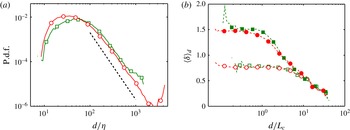
Figure 11. (a) Probability density function of the diagonal size of Q4s for which the nearest Q2 is at $r<d$ . The slope of the dashed line is $-3$ . (b) Mean dimensionless distance, $\langle \unicode[STIX]{x1D6FF}\rangle _{d}$ , defined as in (5.3) for pairs in which the diameter of the reference object is $d$ . In both figures, ▫, M32; ○, H32. Solid symbols are for pairs with $r<2d$ and open ones are for $r<d$ . Only the latter case is plotted in (a) because the two cases are almost indistinguishable.

6.1 The effect of inhomogeneity in channels

Finally, figure 14 compares the structure of the conditional flow fields for the three kinds of Q pairs discussed in this paper. Figure 14(a–c) compares the field of the streamwise velocity in the cross-flow sections. It reveals the increasing effect of inhomogeneity as we move from HST in figure 14(a), to detached channel Q pairs in figure 14(b) and to attached Q pairs in figure 14(c). Figure 14(a,b) is the same as figure 12(a,c), but the three figures have now been scaled to have a similar distance between the average positions of the members of the pairs, and aligned to the same location of their centre of gravity. The main difference between detached channel pairs and HST is that the sweep gets larger than the ejection, presumably because it is coming from layers in which the integral length (proportional to $y$ ) is larger. This difference gets most marked for the attached pairs in figure 14(c), where the high-speed streak of the sweep is considerably larger than the low-speed one (see also LFJ12). Comparing this figure with figure 14(a), it can almost be interpreted that the ejection is truncated by the presence of the impermeable wall. Although not shown in the figure, the high-shear layer of the attached pair is only clearly present above the low-velocity ejection streak. The layer underneath the high-velocity sweep has been absorbed by the high-shear viscous region at the wall. Otherwise, the differences between the three types of structures are relatively minor. In particular, the intensity of the conditional streaks is almost the same in the three cases.

Figure 14(d–f) shows three-dimensional views of the inclined roller mentioned in figure 13(a,b), now shown in relation to the high- and low-velocity streaks. Figure 14(d) reveals that the roller in HST is part of a conditional double ‘hairpin’, containing both an upright and an inverted hook, although it is important to remember that this is a conditional flow structure unlikely to represent any individual flow realisation, and that the roller is formed by the superposition of many small-scale vortices, each of which is almost isotropically oriented. Figure 14(d) shows that this double hairpin straddles both the high- and low-speed streaks in the background of figure 14(a,b), and it is interesting that both streaks extend ‘downstream’ from their respective hairpin end. The high-speed streak starts roughly at the inverted hairpin hook and extends to the right of the figure, while the low-speed streak extends in the opposite direction, starting from the upright hook. It is clear from the figure that the two ‘hooks’ are the high-shear layers whose cross-section was described in figure 12(b) and in § 5.2 as being located respectively above and below the low- and high-velocity streaks. A trivial observation is that the hairpins shown here are not connected to the wall in the wall-less HST flow.

The symmetry of figure 14(d) is a direct consequence of the statistical symmetries of HST. Figure 14(e) presents the same view of the conditional detached Q pairs in the logarithmic layer of the channel. Although less symmetric than in figure 14(d), the two figures are similar enough to strongly suggest that the same mechanisms are at play in both cases. When the plot is drawn for the attached Qs of the channel, the conditional figure is dominated by a strong vorticity layer attached to the wall, defined in this case as $\unicode[STIX]{x1D6FF}_{y}^{\prime }=0$ . Once this layer is removed by truncating the domain (to $\unicode[STIX]{x1D6FF}_{y}^{\prime }>0.15$ in figure 14 f), the roller reappears, although with a much shallower inclination with respect to the mean stream than in the case of Q pairs located farther from the wall. It can best be described as one of the quasi-streamwise vortices of the classical descriptions of the buffer layer (Robinson Reference Robinson1991), although all of the Q pairs in this figure are large $(y_{max}^{+}>100)$ . The present definition of the roller in terms of the magnitude of the conditional vorticity incorporates the wall-parallel shear layer that can be seen in figure 14(f), forming an arch above the low-velocity streak. This layer corresponds to the upright hairpin hook in figure 14(d,e). The asymmetry between the streaks, already clear in figure 14(e), is exaggerated here, with a very large high-speed streak accompanying a much smaller low-speed one, hidden in the plot by the upright hook of the conditional roller. This agrees with the picture of the same case in figure 12(c) of LFJ12. It should be noted that, even in the attached case, there is a residual inverted hook that appears as a small isolated structure to the right of figure 14(f), but which is connected to the rest of the roller by the high-vorticity wall layer that has been removed for clarity.