


1. Introduction
Spontaneous flow reversals occur in various buoyancy-driven fluid dynamical systems (Sugiyama et al. Reference Sugiyama2010; Wang et al. Reference Wang, Lai, Song and Tong2018), such as large-scale flows in the ocean (Nunes & Norris Reference Nunes and Norris2006), the atmosphere (Cai et al. Reference Cai2021), or the inner core of stars or the Earth, where such reversals are associated with the reversal of the magnetic field (Glatzmaier et al. Reference Glatzmaier, Coe, Hongre and Roberts1999). They are characterized by a large range of temporal and spatial scales, high dimensionality, and intermittence. Various models, either of a stochastic nature (Brown & Ahlers Reference Brown and Ahlers2007, Reference Brown and Ahlers2008) or based on simplified (nonlinear) dynamical equations (Araujo, Grossmann & Lohse Reference Araujo, Grossmann and Lohse2005; Chandra & Verma Reference Chandra and Verma2013; Suri Reference Suri2024), have been developed to account for the reversals. However, these models are mostly qualitative or often inaccurate in predicting the reversals. Progress in analysing and manipulating turbulent fluid motion is needed to better predict and control these dynamic structures. This is crucial not only for the reversals in buoyancy-driven flows but also for other problems in which the flow switches between either two competing states or a persistent state and a rare event, such as von Kármán swirling flow (de la Torre & Burguete Reference de la Torre and Burguete2007), rotating spherical Couette flow (Zimmerman, Triana & Lathrop Reference Zimmerman, Triana and Lathrop2011), flow mixing (Schikarski et al. Reference Schikarski, Trzenschiok, Peukert and Avila2019), near-wall turbulence (Jiménez & Moin Reference Jiménez and Moin1991; Jiménez Reference Jiménez2023), pipe flow (Avila, Barkley & Hof Reference Avila, Barkley and Hof2023), zonal flow bursts (von Hardenberg et al. Reference von Hardenberg, Goluskin, Provenzale and Spiegel2015), Taylor–Couette turbulence (Borrero-Echeverry, Schatz & Tagg Reference Borrero-Echeverry, Schatz and Tagg2010) or aerodynamic bifurcation (Gayout, Bourgoin & Plihon Reference Gayout, Bourgoin and Plihon2021).
Data-driven modelling has advanced significantly in recent decades due to algorithmic improvements, increased data availability, and faster hardware. This approach is suitable for modelling intermittent events and is pivotal for physical insight, state estimation from limited data, prediction, control and optimization (Brunton, Noack & Koumoutsakos Reference Brunton, Noack and Koumoutsakos2020). Typically, such modelling relies on a low-dimensional approximation of the state and system identification within that approximation. The commonly used reduced-order modelling methods include proper orthogonal decomposition (POD) (Holmes Reference Holmes2012; Lumey Reference Lumey2012), dynamic mode decomposition (DMD) (Schmid Reference Schmid2010) and Koopman analysis (Mezić Reference Mezić2013; Giannakis et al. Reference Giannakis, Kolchinskaya, Krasnov and Schumacher2018), which can reduce computational costs and extract the dominant flow patterns effectively, and has been applied broadly (Kutz et al. Reference Kutz, Brunton, Brunton and Proctor2016; Kou & Zhang Reference Kou and Zhang2017; Kou, Le Clainche & Zhang Reference Kou, Le Clainche and Zhang2018; Schmid Reference Schmid2022; Yang et al. Reference Yang, Zhang, Reiter, Lohse, Shishkina and Linkmann2022). For Rayleigh–Bénard convection, Podvin and Sergent use POD modes to comprehensively investigate the large-scale circulation (LSC) and the reversal dynamics (Podvin & Sergent Reference Podvin and Sergent2012, Reference Podvin and Sergent2015, Reference Podvin and Sergent2017; Castillo-Castellanos et al. Reference Castillo-Castellanos, Sergent, Podvin and Rossi2019; Soucasse et al. Reference Soucasse, Podvin, Rivière and Soufiani2019) in two- and three-dimensional turbulent convection. Xu, Chen & Xi (Reference Xu, Chen and Xi2021) use POD modes to study the reversal dynamics in two-dimensional circular convection cells, and compare them with the Fourier modes. Chandra & Verma (Reference Chandra and Verma2011) use large-scale Fourier modes, coupled with symmetry transformations, to identify the dynamics of flow reversals.
Recent developments in data-driven modelling include the sparse identification of nonlinear dynamics (SINDy) algorithm, which identifies accurate parsimonious models from data (Brunton, Proctor & Kutz Reference Brunton, Proctor and Kutz2016) but is challenging to scale to large-scale problems due to the size of the associated feature spaces; in addition, we have, among many other models, access to neural network models (Vlachas et al. Reference Vlachas, Byeon, Wan, Sapsis and Koumoutsakos2018) that avoid high computational cost but have limited interpretability and provide little physical insights. An alternative paradigm based on cluster modelling has recently been applied to fluid flows, as it presents a promising course of action for understanding the physics behind complex fluid motions (Kaiser et al. Reference Kaiser2014; Fernex, Noack & Semaan Reference Fernex, Noack and Semaan2021; Deng et al. Reference Deng, Noack, Morzyński and Pastur2022; Hou, Deng & Noack Reference Hou, Deng and Noack2024), including large-scale flow structures in three-dimensional Rayleigh–Bénard convection (Maity et al. Reference Maity, Koltai and Schumacher2022, Reference Maity, Bittracher, Koltai and Schumacher2023), flow past cylinder wakes (Deng et al. Reference Deng, Noack, Morzyński and Pastur2022; Hou et al. Reference Hou, Deng and Noack2024), and Lagrangian vortex dynamics (Hadjighasem et al. Reference Hadjighasem, Karrasch, Teramoto and Haller2016).
In this work, we promote an alternative cluster modelling technique based on a complex network, which explicitly considers the topology of the network and is designed to handle directionality in the patterns of connecting edges between nodes. The main goal of this approach is to leverage a cluster-based framework for better understanding, predicting and potentially controlling intricate flow behaviour. As a model system, we concentrate on two-dimensional turbulent Rayleigh–Bénard convection (Ahlers, Grossmann & Lohse Reference Ahlers, Grossmann and Lohse2009; Lohse & Xia Reference Lohse and Xia2010; Shishkina Reference Shishkina2021; Lohse & Shishkina Reference Lohse and Shishkina2024), consisting of a fluid layer heated from below and cooled from above, where intermittent flow reversals are readily observed (Sugiyama et al. Reference Sugiyama2010; Chandra & Verma Reference Chandra and Verma2013). Starting with a time-resolved snapshot sequence of a trajectory in a high-dimensional phase space spanned by appropriate coherent flow fields (given by e.g. POD modes), the thus reduced-order phase space is discretized, and the resulting trajectory is converted into a Markov matrix describing the transition probabilities between various phase-space elements over one time step. This Markov matrix is subsequently interpreted as a directed, weighted graph (Chartrand & Zhang Reference Chartrand and Zhang2013) consisting of all occupied phase-space elements, encoding the dynamics of the data sequence probabilistically. Different from a $K$
-means clustering algorithm used in previous cluster-based models (Kaiser et al. Reference Kaiser2014; Fernex et al. Reference Fernex, Noack and Semaan2021; Hou et al. Reference Hou, Deng and Noack2024), we reorganize the original network into larger communities, defined as groups of nodes with strong intraconnectivity and weak interconnectivity, to isolate persistent motion from rare outlier events (Newman Reference Newman2006; Leicht & Newman Reference Leicht and Newman2008; Schmid et al. Reference Schmid, Schmidt, Towne and Hack2018). This clustering method has proven itself effective in classifying communities, and makes use of the information contained in the edges, i.e. the links between nodes. An explicit network model of the flow reversals is obtained, which effectively categorizes and predicts the intermittent reversal events. Each of the procedural steps will be further explained in detail.
$K$
-means clustering algorithm used in previous cluster-based models (Kaiser et al. Reference Kaiser2014; Fernex et al. Reference Fernex, Noack and Semaan2021; Hou et al. Reference Hou, Deng and Noack2024), we reorganize the original network into larger communities, defined as groups of nodes with strong intraconnectivity and weak interconnectivity, to isolate persistent motion from rare outlier events (Newman Reference Newman2006; Leicht & Newman Reference Leicht and Newman2008; Schmid et al. Reference Schmid, Schmidt, Towne and Hack2018). This clustering method has proven itself effective in classifying communities, and makes use of the information contained in the edges, i.e. the links between nodes. An explicit network model of the flow reversals is obtained, which effectively categorizes and predicts the intermittent reversal events. Each of the procedural steps will be further explained in detail.
The organization of the paper is as follows. § 2 introduces the flow configuration, including the direct numerical simulations of thermal convection, together with the control and response parameters. § 3 introduces details of the complex-network model and presents results. Conclusions are offered in § 4.
2. Flow configuration
Direct numerical simulations (DNS) for incompressible Oberbeck–Boussinesq flow are performed (Verzicco & Orlandi Reference Verzicco and Orlandi1996), which have been widely used to study thermal convection (Yang et al. Reference Yang, Verzicco and Lohse2016, Reference Yang, Chong, Wang, Verzicco, Shishkina and Lohse2020; Blass et al. Reference Blass, Zhu, Verzicco, Lohse and Stevens2020). The non-dimensionalized governing equations, including the incompressibility condition, are given by
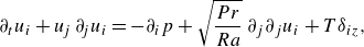 \begin{align} \partial _ { t } u _ { i } + u _{\!j}\, \partial_{\!j } u _ { i } &= - \partial _ { i } p + \sqrt { \frac { P r } { R a } }\, \partial _ { j } \partial _ { j } u _ { i } + T \delta _ { i z }, \end{align}
 \begin{align} \partial _ { t } T + u _ { i }\, \partial _ { i } T &= \frac { 1 } { \sqrt { R a\, P r }}\, \partial_j \partial_j T, \end{align}
 \begin{align} \partial _ { i } u _ { i } &= 0, \end{align}
where $u$
,
$u$
, $T$
and
$T$
and $p$
are the dimensionless velocity, temperature and pressure. The dimensionless control parameters include the Rayleigh number
$p$
are the dimensionless velocity, temperature and pressure. The dimensionless control parameters include the Rayleigh number $Ra=\alpha g H^3\Delta /(\nu \kappa )$
, the Prandtl number
$Ra=\alpha g H^3\Delta /(\nu \kappa )$
, the Prandtl number $Pr=\nu /\kappa$
, and the aspect ratio of the container
$Pr=\nu /\kappa$
, and the aspect ratio of the container $\Gamma$
, where
$\Gamma$
, where $\alpha$
,
$\alpha$
, $\nu$
and
$\nu$
and $\kappa$
denote the thermal expansion coefficient, the kinematic viscosity and the thermal diffusivity of the fluid, respectively. The parameter
$\kappa$
denote the thermal expansion coefficient, the kinematic viscosity and the thermal diffusivity of the fluid, respectively. The parameter $g$
denotes the gravitational acceleration, and
$g$
denotes the gravitational acceleration, and $\varDelta$
stands for the temperature difference between the bottom and top boundaries. The time, lengths and temperature are rendered dimensionless by the free-fall time
$\varDelta$
stands for the temperature difference between the bottom and top boundaries. The time, lengths and temperature are rendered dimensionless by the free-fall time $t_f=\sqrt {H/(\alpha g \Delta )}$
, the free-fall velocity
$t_f=\sqrt {H/(\alpha g \Delta )}$
, the free-fall velocity $U = \sqrt {\alpha g\Delta H}$
, the height
$U = \sqrt {\alpha g\Delta H}$
, the height $H$
of the container, and the temperature difference
$H$
of the container, and the temperature difference $\varDelta$
, respectively. The simulations are conducted in a two-dimensional square box with no-slip and impermeable boundary conditions for all walls. The governing equations in a Cartesian geometry were solved by a second-order finite-difference scheme in space and by a fractional-step third-order Runge–Kutta scheme combined with the Crank–Nicolson scheme for the implicit terms in time (Verzicco & Orlandi Reference Verzicco and Orlandi1996).
$\varDelta$
, respectively. The simulations are conducted in a two-dimensional square box with no-slip and impermeable boundary conditions for all walls. The governing equations in a Cartesian geometry were solved by a second-order finite-difference scheme in space and by a fractional-step third-order Runge–Kutta scheme combined with the Crank–Nicolson scheme for the implicit terms in time (Verzicco & Orlandi Reference Verzicco and Orlandi1996).
Reversals can be detected by the volume-averaged angular momentum about the centre of the box $L$
, which is defined as
$L$
, which is defined as
 \begin{equation} L(t)=\left \langle -(z-H / 2)\, u(x, t)+ (x-H / 2)\, v(x, t)\right \rangle _V, \end{equation}
where $u,v$
are the horizontal and vertical velocities, respectively. Statistics were collected after a sufficiently long start-up to ensure that the flow had reached a quasi-statistical stationary state. Here, we restrict ourselves to the study of flow reversals in a two-dimensional square geometry (
$u,v$
are the horizontal and vertical velocities, respectively. Statistics were collected after a sufficiently long start-up to ensure that the flow had reached a quasi-statistical stationary state. Here, we restrict ourselves to the study of flow reversals in a two-dimensional square geometry ( $\Gamma = 1$
) and span the parameter ranges
$\Gamma = 1$
) and span the parameter ranges $10^6 \le Ra \le 2\times 10^8,\ 3 \le Pr \le 10$
. The numerical details of the simulations are listed in table 1. We choose
$10^6 \le Ra \le 2\times 10^8,\ 3 \le Pr \le 10$
. The numerical details of the simulations are listed in table 1. We choose $Ra=10^8$
and
$Ra=10^8$
and $Pr=4.3$
as the default case, unless otherwise specified. Typical flow structures with a domain-size LSC are shown in figure 1(a) from one simulation but at different time instants. The flow reversal is indicated by the arrow directions.
$Pr=4.3$
as the default case, unless otherwise specified. Typical flow structures with a domain-size LSC are shown in figure 1(a) from one simulation but at different time instants. The flow reversal is indicated by the arrow directions.
Table 1. Simulation parameters and grid information. The columns from left to right indicate the Rayleigh number $Ra$
, the Prandtl number
$Ra$
, the Prandtl number ${Pr}$
, the total simulation time
${Pr}$
, the total simulation time $t_{total}$
in free-fall time units, and the grid information.
$t_{total}$
in free-fall time units, and the grid information.
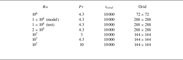
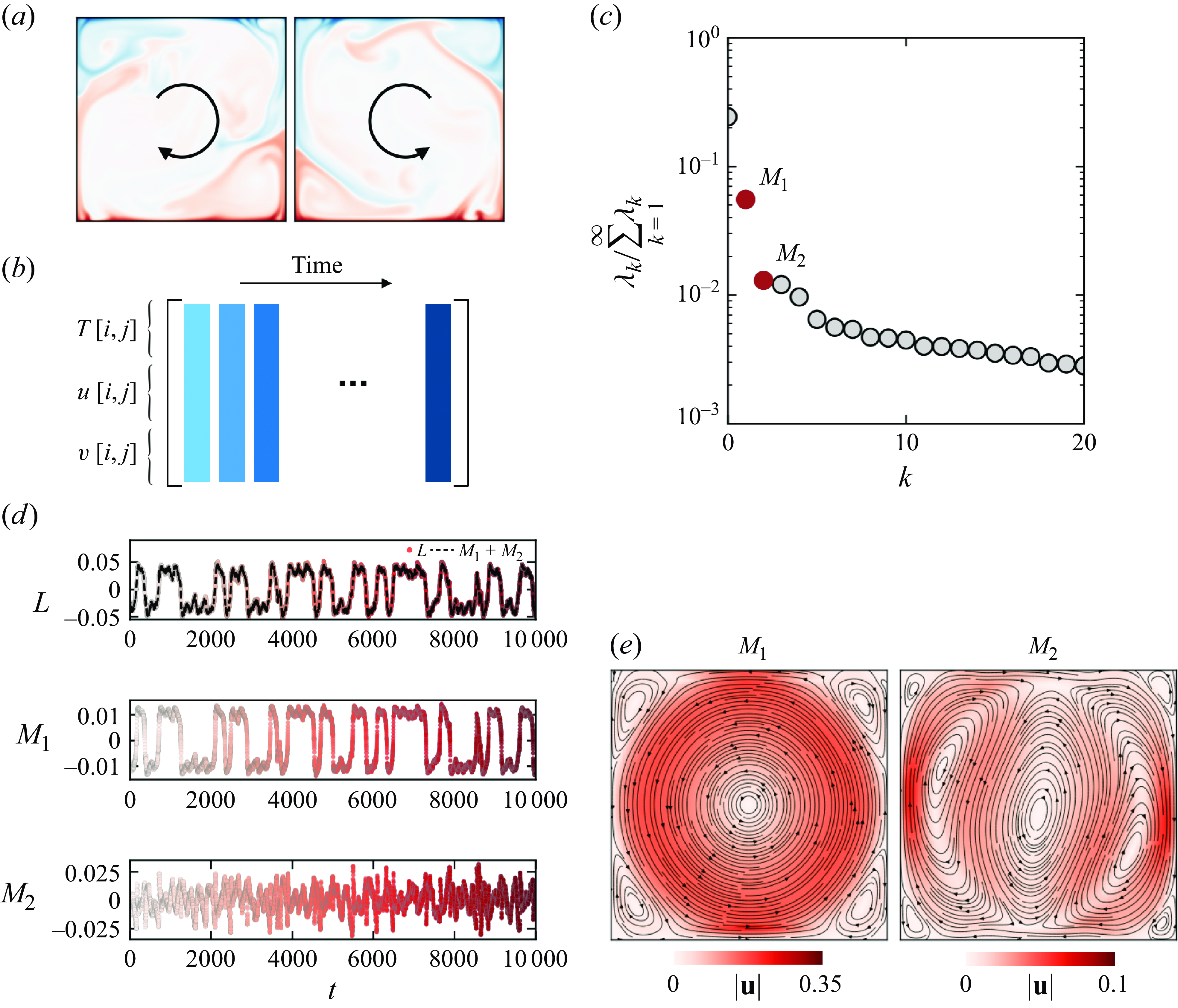
Figure 1. Sketch of the clustering procedure. (a) Temperature fields from the original data; two snapshots show different LSC orientations. (b) Data collection and reorganization into a matrix, including the state variables $T$
,
$T$
, $u$
and
$u$
and $v$
. (c) The normalized magnitude of POD modes in descending order
$v$
. (c) The normalized magnitude of POD modes in descending order $k$
. Here,
$k$
. Here, $M_1$
and
$M_1$
and $M_2$
represent the first two dominant modes after the steady mode at
$M_2$
represent the first two dominant modes after the steady mode at $k=0$
. (d) The time series of the value of
$k=0$
. (d) The time series of the value of $L$
and the first two POD modes
$L$
and the first two POD modes $M_1$
and
$M_1$
and $M_2$
. The dashed line in the plot of
$M_2$
. The dashed line in the plot of $L$
represents the reconstructed
$L$
represents the reconstructed $L'$
from
$L'$
from $M_1$
and
$M_1$
and $M_2$
. (e) The reconstructed velocity magnitude field based on
$M_2$
. (e) The reconstructed velocity magnitude field based on $M_1$
and
$M_1$
and $M_2$
; the velocity direction is shown by streamlines.
$M_2$
; the velocity direction is shown by streamlines.
3. Complex-network modelling and results
3.1. Dimensionality reduction by phase-space embedding
The first step in our approach is to project the original dataset onto a lower-dimensional space, which is an optional process but significantly reduces the overall computational costs. We choose the POD modes (Holmes Reference Holmes2012; Lumey Reference Lumey2012) as a convenient starting point. The output frequency of the temperature and velocity fields is linked to one free-fall time unit. This choice ensures that we have sufficient data points to capture the transient reversal process. Selecting a time step that is too large would result in a loss of information regarding the transition, and could compromise the quality of the clustering analysis. By downsampling and projecting the original flow fields (consisting of temperature $T$
and velocity
$T$
and velocity $u, v$
fields collected into a composite data matrix; see figure 1
b) onto the retained POD modes, we obtain a time series for the expansion coefficients.
$u, v$
fields collected into a composite data matrix; see figure 1
b) onto the retained POD modes, we obtain a time series for the expansion coefficients.
Figure 1(c) shows the magnitude of POD modes, in descending order and numbered by $k$
. The first mode (
$k$
. The first mode ( $k=0$
) is the steady mode representing the mean field, and the following two modes,
$k=0$
) is the steady mode representing the mean field, and the following two modes, $M_1$
and
$M_1$
and $M_2$
, are the dominant modes contributing to the flow reversal. Figure 1(d) shows the time series of
$M_2$
, are the dominant modes contributing to the flow reversal. Figure 1(d) shows the time series of $L$
,
$L$
, $M_1$
and
$M_1$
and $M_2$
. Surprisingly, the reconstructed angular momentum
$M_2$
. Surprisingly, the reconstructed angular momentum $L'$
, based on
$L'$
, based on $M_1$
and
$M_1$
and $M_2$
only, can well reproduce the original
$M_2$
only, can well reproduce the original $L$
, indicating that it suffices to consider only the first two POD modes, beyond the mean flow mode. More details on other POD modes are described in Appendix A. From the temporal evolution of
$L$
, indicating that it suffices to consider only the first two POD modes, beyond the mean flow mode. More details on other POD modes are described in Appendix A. From the temporal evolution of $L$
, one can clearly detect the random and intermittent occurrence of reversals of the LSC orientation. Such reversal events have been found to obey a Poisson process, i.e. successive reversal events are independent of each other (see Xi & Xia Reference Xi and Xia2007).
$L$
, one can clearly detect the random and intermittent occurrence of reversals of the LSC orientation. Such reversal events have been found to obey a Poisson process, i.e. successive reversal events are independent of each other (see Xi & Xia Reference Xi and Xia2007).
Figure 1(e) shows the reconstructed flow field based on $M_1$
and
$M_1$
and $M_2$
, where
$M_2$
, where $M_1$
stands for the single-roll structure with the changing of sign representing the flow reversal, and
$M_1$
stands for the single-roll structure with the changing of sign representing the flow reversal, and $M_2$
corresponds to the three-roll flow structure. The two-dimensional phase space of
$M_2$
corresponds to the three-roll flow structure. The two-dimensional phase space of $M_1$
and
$M_1$
and $M_2$
is displayed in figure 2(a). We observe two distinct regions representing stable LSCs with different directions, and the centre region capturing the transitions between the two stable LSCs. We also checked that higher-order phase-space modes describe noisy signals and do not contribute additional information beyond the two retained modes. A video of the temporal evolution process of the POD phase space can be found in the supplementary material (available at https://doi.org/10.1017/jfm.2025.371).
$M_2$
is displayed in figure 2(a). We observe two distinct regions representing stable LSCs with different directions, and the centre region capturing the transitions between the two stable LSCs. We also checked that higher-order phase-space modes describe noisy signals and do not contribute additional information beyond the two retained modes. A video of the temporal evolution process of the POD phase space can be found in the supplementary material (available at https://doi.org/10.1017/jfm.2025.371).
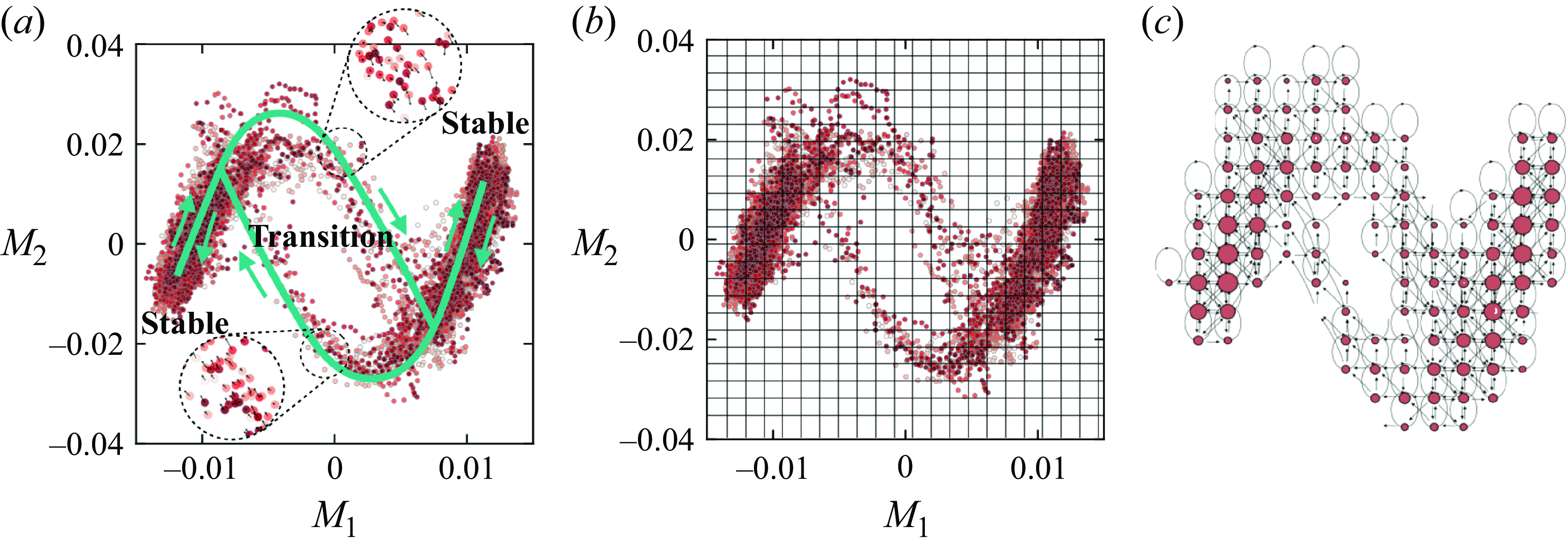
Figure 2. (a) Phase space spanned by the two dominant POD coefficients $M_1$
and
$M_1$
and $M_2$
, each point representing one instant in time. The cyan lines show the direction of the motion. (b) An illustration of the discretized network of the phase space from (a). (c) The final complex network based on (3.3) with
$M_2$
, each point representing one instant in time. The cyan lines show the direction of the motion. (b) An illustration of the discretized network of the phase space from (a). (c) The final complex network based on (3.3) with $N=30.$
The circles represent nodes, with the size indicating the density. The arrows represent the edges.
$N=30.$
The circles represent nodes, with the size indicating the density. The arrows represent the edges.
3.2. Constructing the Markov matrix
Following the phase-space trajectory in the lower-dimensional representation of the flow reversal, we proceed by discretizing the phase space to estimate transition probabilities. A straightforward and efficient discretization uses rectangular boxes (more generally hypercubes for phase spaces of any dimension) and a counting measure. More formally, we denote the set of box elements from our discretization by $\{B_1, \ldots, B_N\}$
, where
$\{B_1, \ldots, B_N\}$
, where $N$
denotes the number of boxes, and write the indicator function for
$N$
denotes the number of boxes, and write the indicator function for $B_i$
as
$B_i$
as
 \begin{equation} \mathbb{I}_{B_i(x)}=\left \{\begin{array}{ll} 1, & \text{if } x \in B_i, \\[4pt] 0, & \text{otherwise. } \end{array}\right . \end{equation}
We further introduce a suitable density measure $m(B_i)$
for each box
$m(B_i)$
for each box $B_i$
, which we take as the number of instances (phase-space points) that it contains, and a continuous operator
$B_i$
, which we take as the number of instances (phase-space points) that it contains, and a continuous operator $\mathcal{P}$
that describes the transition probabilities between phase-space elements. A Galerkin projection of
$\mathcal{P}$
that describes the transition probabilities between phase-space elements. A Galerkin projection of $\mathcal{P}$
onto a subspace spanned by the indicator function is expressed by
$\mathcal{P}$
onto a subspace spanned by the indicator function is expressed by
 \begin{equation} \int \mathbb{I}_{\mathrm{B}_{\!j}} \mathcal{P}\, \ \mathbb{I}_{\mathrm{B}_i}\, {\textrm d}m = m \left ({B}_i \cap \mathcal{F}^{-1} \left ({B}_{\!j}\right ) \right ). \end{equation}
The resulting transition probability matrix $P$
can be defined by its elements according to
$P$
can be defined by its elements according to
 \begin{equation} {P}_{i j}=\frac {m\left ({B}_i \cap \mathcal{F}^{-1}\left ({B}_{\!j}\right )\right )}{m\left ({B}_i\right )}, \quad i, j=1, \ldots, N, \end{equation}
where $\mathcal{F}^{-1}$
denotes the temporal backstep operator, i.e. we evaluate its argument at the previous time step, which is identical to the original data interval for a time-discrete formulation. The numerator in (3.3) represents the number of transitions into box
$\mathcal{F}^{-1}$
denotes the temporal backstep operator, i.e. we evaluate its argument at the previous time step, which is identical to the original data interval for a time-discrete formulation. The numerator in (3.3) represents the number of transitions into box $B_i$
from box
$B_i$
from box $B_j$
over a single time step, while the denominator denotes the total number of states located within the box
$B_j$
over a single time step, while the denominator denotes the total number of states located within the box $B_i$
. The ratio approximates the Markov transition probability between boxes
$B_i$
. The ratio approximates the Markov transition probability between boxes $B_j$
and
$B_j$
and $B_i$
. The complete matrix
$B_i$
. The complete matrix $P$
furnishes an approximation of the Markov transition probability matrix for all boxes in our phase-space discretization. Our particular discretization is referred to as the Ulam–Galerkin method (Ulam Reference Ulam1960; Li Reference Li1976; Kaiser et al. Reference Kaiser2014). Mathematically, this matrix
$P$
furnishes an approximation of the Markov transition probability matrix for all boxes in our phase-space discretization. Our particular discretization is referred to as the Ulam–Galerkin method (Ulam Reference Ulam1960; Li Reference Li1976; Kaiser et al. Reference Kaiser2014). Mathematically, this matrix $P$
constitutes a finite-dimensional approximation of the Frobenius–Perron operator – the adjoint of the Koopman operator (Lasota & Mackey Reference Lasota and Mackey2013; Kaiser et al. Reference Kaiser2014). The above approximation of the Frobenius–Perron operator can be thought of as the analogue of the DMD matrix for approximating the Koopman operator.
$P$
constitutes a finite-dimensional approximation of the Frobenius–Perron operator – the adjoint of the Koopman operator (Lasota & Mackey Reference Lasota and Mackey2013; Kaiser et al. Reference Kaiser2014). The above approximation of the Frobenius–Perron operator can be thought of as the analogue of the DMD matrix for approximating the Koopman operator.
We use a discretization with $24$
boxes in each direction, which yields
$24$
boxes in each direction, which yields $257$
cells in total; see the illustration in figure 2(b). The result of the discretized phase space is shown in figure 2(c): the circles represent nodes in the network, with the size indicating local measure density, and the arrows represent the edges indicating the cell-to-cell transitions. The network reveals two stable regions characterized by larger nodes. Before proceeding with our analysis, it is important to note that the resolution of the phase-space discretization remains an adjustable parameter in our study. A low-resolution discretization leads to too few communities and may lose pertinent information about the transition regions. A high-resolution discretization, on the other hand, identifies too many independent communities and noisy signals, since the data points that fall inside the control volumes are far too sparse. A more detailed discussion of balancing these two extreme cases is included in the Appendix B. For our case, we choose a proper resolution of the phase-space trajectory that yields a suitable number of communities.
$257$
cells in total; see the illustration in figure 2(b). The result of the discretized phase space is shown in figure 2(c): the circles represent nodes in the network, with the size indicating local measure density, and the arrows represent the edges indicating the cell-to-cell transitions. The network reveals two stable regions characterized by larger nodes. Before proceeding with our analysis, it is important to note that the resolution of the phase-space discretization remains an adjustable parameter in our study. A low-resolution discretization leads to too few communities and may lose pertinent information about the transition regions. A high-resolution discretization, on the other hand, identifies too many independent communities and noisy signals, since the data points that fall inside the control volumes are far too sparse. A more detailed discussion of balancing these two extreme cases is included in the Appendix B. For our case, we choose a proper resolution of the phase-space trajectory that yields a suitable number of communities.
3.3. Community clustering
To regroup the network into coherent clusters, we define a community as a collection of nodes that exhibits strong intraconnectivity (within the community) but weak interconnectivity (to other communities). Several algorithms are available for detecting graph communities within large networks, many of which use a measure of interconnectivity referred to as modularity (Newman Reference Newman2006; Leicht & Newman Reference Leicht and Newman2008; Schmid et al. Reference Schmid, Schmidt, Towne and Hack2018) and defined as
 \begin{equation} Q=\frac {1}{N} \sum _{i, j}\left [{P}_{i j}-\frac {k_i^{{in }} k_{\!j}^{{out }}}{N}\right ] \delta _{c_i, c_{\!j}} \end{equation}
where $k^{in,out}_i$
represents the in-degree (the number of edges that point into the node) or out-degree (the number of edges that point out from the node) of the
$k^{in,out}_i$
represents the in-degree (the number of edges that point into the node) or out-degree (the number of edges that point out from the node) of the $i$
th node, and
$i$
th node, and $c_i$
denotes the
$c_i$
denotes the $i$
th community. The Kronecker symbol is represented by
$i$
th community. The Kronecker symbol is represented by $\delta _{i,j}.$
Based on this definition, we seek a partition of the graph into communities
$\delta _{i,j}.$
Based on this definition, we seek a partition of the graph into communities $c_i$
such that
$c_i$
such that $Q$
attains a maximum value. To this end, we employ a modularity-based approximation algorithm (Leicht & Newman Reference Leicht and Newman2008), which incrementally improves the modularity
$Q$
attains a maximum value. To this end, we employ a modularity-based approximation algorithm (Leicht & Newman Reference Leicht and Newman2008), which incrementally improves the modularity $Q$
by exploiting the spectral properties of the graph; it is computationally efficient, and produces good and robust results in practice (Danon et al. Reference Danon, Diaz-Guilera, Duch and Arenas2005; Leicht & Newman Reference Leicht and Newman2008).
$Q$
by exploiting the spectral properties of the graph; it is computationally efficient, and produces good and robust results in practice (Danon et al. Reference Danon, Diaz-Guilera, Duch and Arenas2005; Leicht & Newman Reference Leicht and Newman2008).
Starting with a simplified configuration with only two communities, we define $s_i$
to be
$s_i$
to be $+1$
when
$+1$
when $i$
is in the first community, and
$i$
is in the first community, and $-1$
if it is in the second community. Then
$-1$
if it is in the second community. Then $\delta _{c_i, c_{\!j}}$
can be represented by
$\delta _{c_i, c_{\!j}}$
can be represented by $1/2(s_i s_{\!j} + 1)$
, and (3.4) can be rewritten as
$1/2(s_i s_{\!j} + 1)$
, and (3.4) can be rewritten as
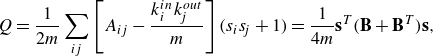 \begin{equation} Q=\frac {1}{2m}\sum _{ij}\left [A_{ij}-\frac {k_i^{{in}}k_{\!j}^{{out}}}{m}\right ](s_is_{\!j}+1)=\frac {1}{4m}{\textbf{s}}^{{T}}({\textbf{B}}+{\textbf{B}}^{{T}}){\textbf{s}}, \end{equation}
where $\textbf{s}$
is the vector form of
$\textbf{s}$
is the vector form of $s_i$
, and
$s_i$
, and $\textbf{B}$
is the so-called modularity matrix, whose entries are defined as
$\textbf{B}$
is the so-called modularity matrix, whose entries are defined as
 \begin{equation} B_{ij}=A_{ij}-\frac {k_i^{{in}}k_{\!j}^{{out}}}{m}. \end{equation}
The goal is then to find the vector $\boldsymbol{s}$
that maximizes
$\boldsymbol{s}$
that maximizes $Q$
for a given
$Q$
for a given $\textbf{B}$
. In the algorithm, the eigenvector corresponding to the largest positive eigenvalue of the symmetric matrix
$\textbf{B}$
. In the algorithm, the eigenvector corresponding to the largest positive eigenvalue of the symmetric matrix $\textbf{B}+\textbf{B}^{\mathrm T}$
is calculated, after which communities are assigned based on the signs of the elements of this eigenvector. The reasoning behind this procedural step is the goal to align
$\textbf{B}+\textbf{B}^{\mathrm T}$
is calculated, after which communities are assigned based on the signs of the elements of this eigenvector. The reasoning behind this procedural step is the goal to align $\boldsymbol{s}$
maximally parallel to the leading eigenvector of
$\boldsymbol{s}$
maximally parallel to the leading eigenvector of $\textbf{B}+\textbf{B}^{\mathrm T}$
(Leicht & Newman Reference Leicht and Newman2008). Scaling to more than two communities, we follow a simple course: we first divide the network into two communities, then subdivide those communities, and so on, until we reach a point where further divisions no longer increase
$\textbf{B}+\textbf{B}^{\mathrm T}$
(Leicht & Newman Reference Leicht and Newman2008). Scaling to more than two communities, we follow a simple course: we first divide the network into two communities, then subdivide those communities, and so on, until we reach a point where further divisions no longer increase $Q$
. A more detailed description of the clustering process can be found in Newman (Reference Newman2006) and Leicht & Newman (Reference Leicht and Newman2008).
$Q$
. A more detailed description of the clustering process can be found in Newman (Reference Newman2006) and Leicht & Newman (Reference Leicht and Newman2008).
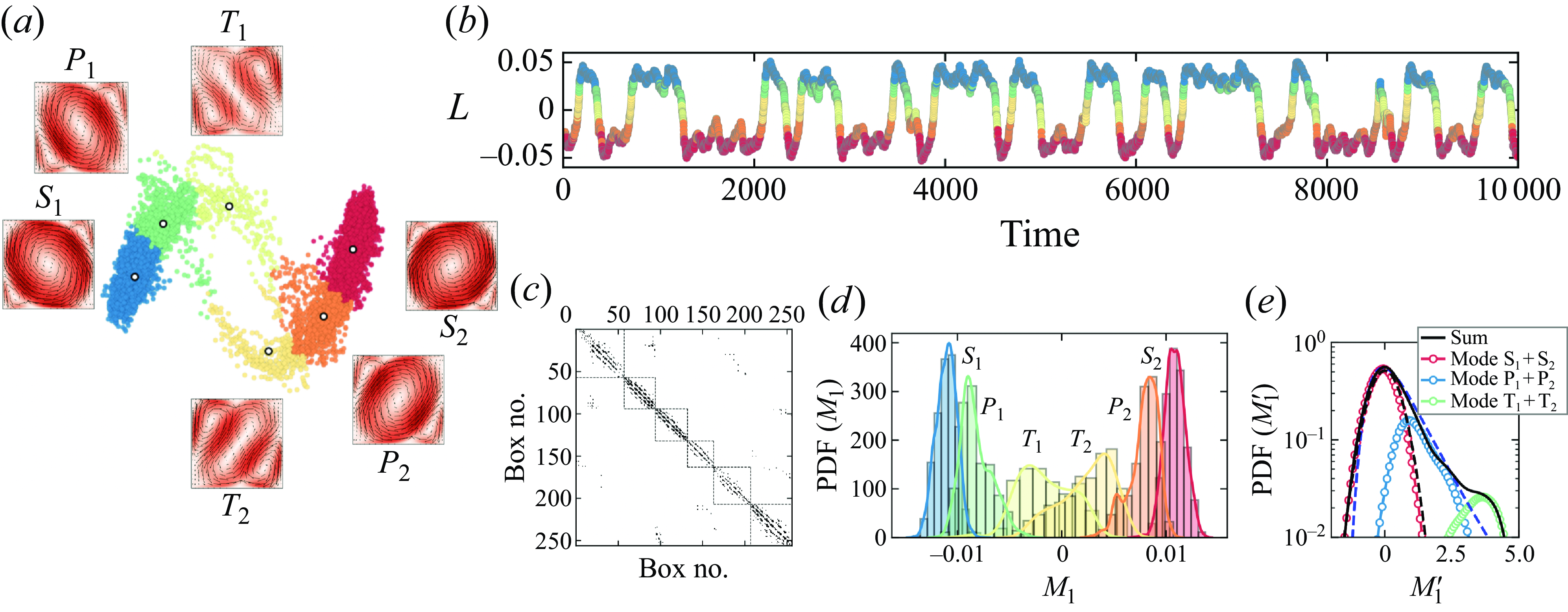
Figure 3. (a) The phase space of $M_1$
and
$M_1$
and $M_2$
, with colours representing different communities, identified based on (3.4). The symbols mark the centroids of each community, and the snapshots show the averaged velocity magnitudes field in the communities. (b) The time series of
$M_2$
, with colours representing different communities, identified based on (3.4). The symbols mark the centroids of each community, and the snapshots show the averaged velocity magnitudes field in the communities. (b) The time series of $L$
, with the colours representing different communities. (c) Fill pattern of the transition probability matrix after applying the clustering algorithm, displaying six distinct communities. (d) Separated PDF of
$L$
, with the colours representing different communities. (c) Fill pattern of the transition probability matrix after applying the clustering algorithm, displaying six distinct communities. (d) Separated PDF of $M_1$
for each community. (e) The PDF of
$M_1$
for each community. (e) The PDF of $M_1'$
for composite symmetric modes. The dashed lines represent Gaussian distributions and the extreme value distribution (Wang et al. Reference Wang, Lai, Song and Tong2018).
$M_1'$
for composite symmetric modes. The dashed lines represent Gaussian distributions and the extreme value distribution (Wang et al. Reference Wang, Lai, Song and Tong2018).
By applying community clustering on the POD-reduced data of flow reversals, we obtained six distinct communities, as depicted in figure 3(a), along with the centroid-averaged flow field for each community. These communities include (i) two stable communities ( $S_1, S_2$
) where the LSC dominates and the flow state is stable, (ii) two precursor communities (
$S_1, S_2$
) where the LSC dominates and the flow state is stable, (ii) two precursor communities ( $P_1, P_2$
) where the LSC is weaker but nonetheless sustained, and (iii) two transition communities (
$P_1, P_2$
) where the LSC is weaker but nonetheless sustained, and (iii) two transition communities ( $T_1, T_2$
) where the LSC breaks down and the flow-state switches from one direction to the opposite. The precursor community is named based on the fact that the trajectory must pass through
$T_1, T_2$
) where the LSC breaks down and the flow-state switches from one direction to the opposite. The precursor community is named based on the fact that the trajectory must pass through $P_1$
or
$P_1$
or $P_2$
in a reversal event. Consequently, the transition from
$P_2$
in a reversal event. Consequently, the transition from $P_1$
(
$P_1$
( $P_2$
) to
$P_2$
) to $T_1$
(
$T_1$
( $T_2$
) carries information that signals the initiation of a reversal. In our following predictions, we also use this precursor information as the start of a reversal. Our method explicitly accounts for the network’s topology and is particularly suited to handle directionality in the patterns of edges between nodes, which the
$T_2$
) carries information that signals the initiation of a reversal. In our following predictions, we also use this precursor information as the start of a reversal. Our method explicitly accounts for the network’s topology and is particularly suited to handle directionality in the patterns of edges between nodes, which the $K$
-means algorithm neglects. To further illustrate this difference, we provide a comparison of results from a
$K$
-means algorithm neglects. To further illustrate this difference, we provide a comparison of results from a $K$
-means clustering method and from our modularity-based method in Appendix C.
$K$
-means clustering method and from our modularity-based method in Appendix C.
Figure 3(b) shows the time series of $L$
, with different colours representing different communities. By retaining the identities of the original snapshots within each community, we reorganize the original transition probability matrix
$L$
, with different colours representing different communities. By retaining the identities of the original snapshots within each community, we reorganize the original transition probability matrix $P$
into a block diagonal form. The dense blocks on the diagonal describe motion within each community, while the sparse off-diagonal blocks represent transitions between communities. The fill pattern of the
$P$
into a block diagonal form. The dense blocks on the diagonal describe motion within each community, while the sparse off-diagonal blocks represent transitions between communities. The fill pattern of the $257 \times 257$
transition matrix, shown in figure 3(c), highlights the six diagonal blocks representing the distinct communities. The fill pattern represents the presence or absence of edges between nodes in a graph, and helps us to visualize the connectivity of the graph. A non-zero entry (black points in figure 3
c) at position
$257 \times 257$
transition matrix, shown in figure 3(c), highlights the six diagonal blocks representing the distinct communities. The fill pattern represents the presence or absence of edges between nodes in a graph, and helps us to visualize the connectivity of the graph. A non-zero entry (black points in figure 3
c) at position $(i,j)$
indicates an edge between nodes
$(i,j)$
indicates an edge between nodes $i$
and
$i$
and $j$
, while a zero indicates no link. The dashed boxes represent the identified communities based on (3.4). The on-diagonal points indicate that the state stays in the same node, the near-diagonal points within each box show a strong connectivity among different nodes in the same community, and the sparse points outside boxes indicate connections between different communities, including precursor and transition states. These precursor structures could be targeted for effective control efforts to prevent reversals, thereby maintaining the system in a single direction of LSC.
$j$
, while a zero indicates no link. The dashed boxes represent the identified communities based on (3.4). The on-diagonal points indicate that the state stays in the same node, the near-diagonal points within each box show a strong connectivity among different nodes in the same community, and the sparse points outside boxes indicate connections between different communities, including precursor and transition states. These precursor structures could be targeted for effective control efforts to prevent reversals, thereby maintaining the system in a single direction of LSC.
We further analyse the probability distribution of $M_1$
for each community in figure 3(d). Stable communities exhibit a steeper curve and shorter tail, while transition communities show a much broader distribution. Combining the symmetric communities, we plot the probability density function (PDF) in figure 3(e), which shows that the stable communities follow a Gaussian distribution, whereas the precursor communities contribute to the long tail of the extreme value distribution. This behaviour can be well described by the generalized extreme-value distribution function (Lucarini et al. Reference Lucarini2016; Wang et al. Reference Wang, Lai, Song and Tong2018)
$M_1$
for each community in figure 3(d). Stable communities exhibit a steeper curve and shorter tail, while transition communities show a much broader distribution. Combining the symmetric communities, we plot the probability density function (PDF) in figure 3(e), which shows that the stable communities follow a Gaussian distribution, whereas the precursor communities contribute to the long tail of the extreme value distribution. This behaviour can be well described by the generalized extreme-value distribution function (Lucarini et al. Reference Lucarini2016; Wang et al. Reference Wang, Lai, Song and Tong2018)
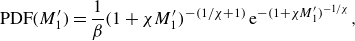 \begin{equation} \mathrm {PDF}( {M}_1^{\prime})=\frac {1}{\beta }(1+\chi {M}_1^{\prime})^{-(1 / \chi +1)}\, {\mathrm e}^{-(1+\chi {M}_1^{\prime})^{-1 / \chi }}, \end{equation}
where $M_1^{\prime}=(M_1-\mu )/\beta$
, the variable
$M_1^{\prime}=(M_1-\mu )/\beta$
, the variable $\chi$
denotes the shape parameter, set to
$\chi$
denotes the shape parameter, set to $\chi =0.1$
, and
$\chi =0.1$
, and $\mu (\chi )$
and
$\mu (\chi )$
and $\beta (\chi )$
are both functions of
$\beta (\chi )$
are both functions of $\chi$
(for details, see Lucarini et al. Reference Lucarini2016; Wang et al. Reference Wang, Lai, Song and Tong2018). This distribution aligns with the previous observations of the reversal statistics (Wang et al. Reference Wang, Lai, Song and Tong2018), and the classification successfully delineates the precursor and transition states from the stable states – another demonstration of the effectiveness of the cluster model.
$\chi$
(for details, see Lucarini et al. Reference Lucarini2016; Wang et al. Reference Wang, Lai, Song and Tong2018). This distribution aligns with the previous observations of the reversal statistics (Wang et al. Reference Wang, Lai, Song and Tong2018), and the classification successfully delineates the precursor and transition states from the stable states – another demonstration of the effectiveness of the cluster model.
3.4. Prediction based on the Markov matrix
Given that the Markov matrix describes the probabilities of transition between various phase-space elements over one time step, it can be used to predict flow reversals by calculating the transition probability for subsequent time steps as follows:
 \begin{equation} {\boldsymbol a}_{t+1,i}=\left \{\begin{array}{ll} 1,& \text{if } {\boldsymbol a}{_t} {P}\ \text{is max at }i, \\[4pt] 0, & \text{otherwise. } \end{array}\right . \end{equation}
Here, $\boldsymbol a$
is the state vector with unity at the current state, and zeros at all other states, and the index ranges from
$\boldsymbol a$
is the state vector with unity at the current state, and zeros at all other states, and the index ranges from $i=1$
to
$i=1$
to $i=257$
, which covers the total number of possible states (nodes). The next state is determined by the transition route with the highest probability among all possible paths, given an initial state with
$i=257$
, which covers the total number of possible states (nodes). The next state is determined by the transition route with the highest probability among all possible paths, given an initial state with $x_0=[0,0,\ldots, 1,0,\ldots, 0]$
, where the location of the coefficient
$x_0=[0,0,\ldots, 1,0,\ldots, 0]$
, where the location of the coefficient $1$
represents the location of the initial state. We compute the next state using the Markov matrix to obtain the probability vector
$1$
represents the location of the initial state. We compute the next state using the Markov matrix to obtain the probability vector $[P_1, P_2,\ldots, P_N]$
. This vector represents the probability of the state location at the next step. We then update the state by selecting the location with the highest probability in the vector, e.g.
$[P_1, P_2,\ldots, P_N]$
. This vector represents the probability of the state location at the next step. We then update the state by selecting the location with the highest probability in the vector, e.g. $P_i$
, and then reset the state as
$P_i$
, and then reset the state as $x_1=[0,0,\ldots, 1,0,\ldots, 0]$
, where
$x_1=[0,0,\ldots, 1,0,\ldots, 0]$
, where $1$
is located at
$1$
is located at $i$
. This updated state is then used for subsequent calculations.
$i$
. This updated state is then used for subsequent calculations.
Using this approach, the state traverses the phase space. We first build the cluster model (Markov matrix) using a test dataset with $10\,000$
snapshots, then apply this model to a new dataset with another
$10\,000$
snapshots, then apply this model to a new dataset with another $10\,000$
snapshots. If we rely solely on the above method, then the state will eventually converge to the stable communities (which are always characterized by the highest probabilities). This results in the model’s failure to capture rare reversal states. To overcome this limitation, we introduce a simple correction to the state before the reversal starts, denoted as
$10\,000$
snapshots. If we rely solely on the above method, then the state will eventually converge to the stable communities (which are always characterized by the highest probabilities). This results in the model’s failure to capture rare reversal states. To overcome this limitation, we introduce a simple correction to the state before the reversal starts, denoted as $t_{corr}$
. The correction scheme adjusts the predicted state from the stable community to the actual state near the transition community in phase space at
$t_{corr}$
. The correction scheme adjusts the predicted state from the stable community to the actual state near the transition community in phase space at $t_{corr}$
. After this correction, the state evolves again following the Markov matrix (as described in (3.8)), until it once more reaches the next reversal. We define
$t_{corr}$
. After this correction, the state evolves again following the Markov matrix (as described in (3.8)), until it once more reaches the next reversal. We define $t_{tran}$
as the time when the actual state is in a precursor community and is moving to a transition community at the next step. To assess the effect of the corrective time
$t_{tran}$
as the time when the actual state is in a precursor community and is moving to a transition community at the next step. To assess the effect of the corrective time $t_{corr}$
relative to
$t_{corr}$
relative to $t_{tran}$
, we introduce the shift time
$t_{tran}$
, we introduce the shift time $\tau =t_{tran} -t_{corr}$
. A value
$\tau =t_{tran} -t_{corr}$
. A value $\tau =0$
implies that the correction is applied right when the state switches to the transition community at the next step. The prediction accuracy (or, more specifically, the fraction of successful predictions; Farazmand & Sapsis Reference Farazmand and Sapsis2017; Vela-Martín & Avila Reference Vela-Martín and Avila2024) is defined as
$\tau =0$
implies that the correction is applied right when the state switches to the transition community at the next step. The prediction accuracy (or, more specifically, the fraction of successful predictions; Farazmand & Sapsis Reference Farazmand and Sapsis2017; Vela-Martín & Avila Reference Vela-Martín and Avila2024) is defined as $N_{m}/N_{t}$
, where
$N_{m}/N_{t}$
, where $N_{m}$
denotes the number of correctly matched reversal events between the actual reversal of mode
$N_{m}$
denotes the number of correctly matched reversal events between the actual reversal of mode $M_1$
and the predicted reversal, which is determined by the change in sign of
$M_1$
and the predicted reversal, which is determined by the change in sign of $M_1$
; the denominator
$M_1$
; the denominator $N_{t}$
represents the total number of predicted reversals.
$N_{t}$
represents the total number of predicted reversals.
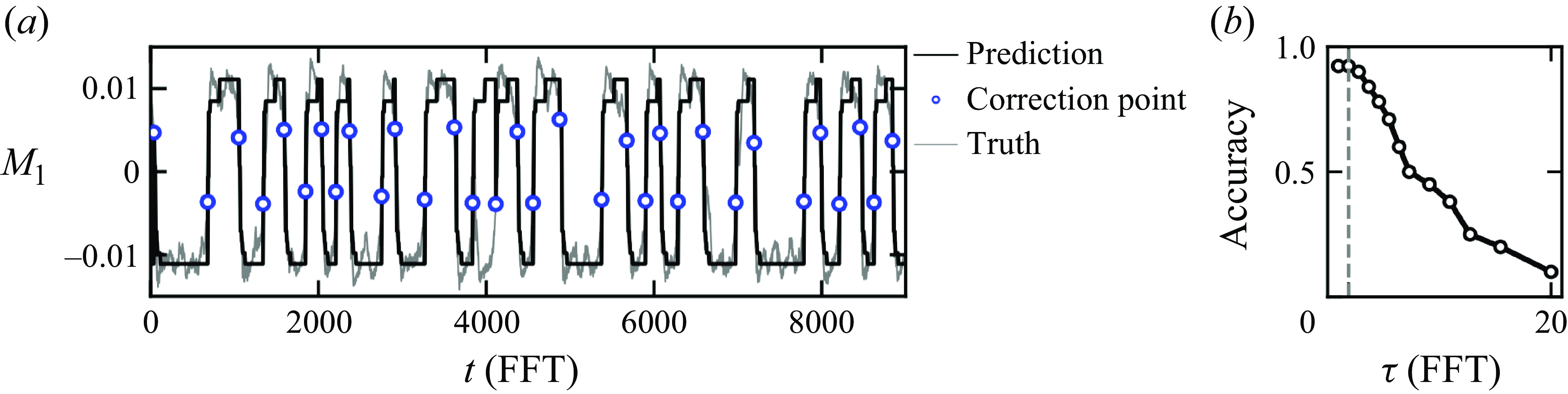
Figure 4. Test of the predictability of the cluster model. (a) The grey line shows the time series of $M_1$
for the test dataset, and the black line shows the prediction based on the Markov matrix and (3.8). The blue symbols represent the locations when a correction is added. (b) The accuracy of prediction as a function of the shift time
$M_1$
for the test dataset, and the black line shows the prediction based on the Markov matrix and (3.8). The blue symbols represent the locations when a correction is added. (b) The accuracy of prediction as a function of the shift time $\tau$
.
$\tau$
.
The prediction results, shown in figure 4(a), demonstrate that the cluster model accurately captures the reversals even for the new (unseen) data. Further analysis reveals that the prediction accuracy peaks at approximately $92\,\%$
when using
$92\,\%$
when using $t_{ {tran}}$
for corrections – and starts to decrease if the correction is applied earlier than
$t_{ {tran}}$
for corrections – and starts to decrease if the correction is applied earlier than $t_{{tran}}$
, as shown in figure 4(b). High prediction accuracy is achieved primarily when the system is near a transition point (
$t_{{tran}}$
, as shown in figure 4(b). High prediction accuracy is achieved primarily when the system is near a transition point ( $\tau \to 0$
). This is due to strong fluctuations in the
$\tau \to 0$
). This is due to strong fluctuations in the $L(t)$
evolution curve. Occasionally,
$L(t)$
evolution curve. Occasionally, $L$
exhibits a drop without leading to a subsequent transition, which complicates the identification of real reversals. As a result, the prediction accuracy tends to diminish when attempting to predict upstream of a transition. Nonetheless, we found that
$L$
exhibits a drop without leading to a subsequent transition, which complicates the identification of real reversals. As a result, the prediction accuracy tends to diminish when attempting to predict upstream of a transition. Nonetheless, we found that $t_{tran}$
is a good indicator and provides useful insight into how far in advance of a transition an accurate prediction of a reversal process is possible. We also compared the prediction of reversals from our model and from a simple threshold-based approach that uses an arbitrary value of
$t_{tran}$
is a good indicator and provides useful insight into how far in advance of a transition an accurate prediction of a reversal process is possible. We also compared the prediction of reversals from our model and from a simple threshold-based approach that uses an arbitrary value of $|L|$
(see Appendix D). The results demonstrate that the identified community structure provides a basis for a meaningful prediction of likely reversals, which can potentially be used for effective control strategies for the reversal processes (Zhang et al. Reference Zhang, Xia, Zhou and Chen2020; Zhao et al. Reference Zhao, Wang, Wu, Chong and Zhou2022; Guo et al. Reference Guo, Wu, Wang, Zhou and Chong2023).
$|L|$
(see Appendix D). The results demonstrate that the identified community structure provides a basis for a meaningful prediction of likely reversals, which can potentially be used for effective control strategies for the reversal processes (Zhang et al. Reference Zhang, Xia, Zhou and Chen2020; Zhao et al. Reference Zhao, Wang, Wu, Chong and Zhou2022; Guo et al. Reference Guo, Wu, Wang, Zhou and Chong2023).
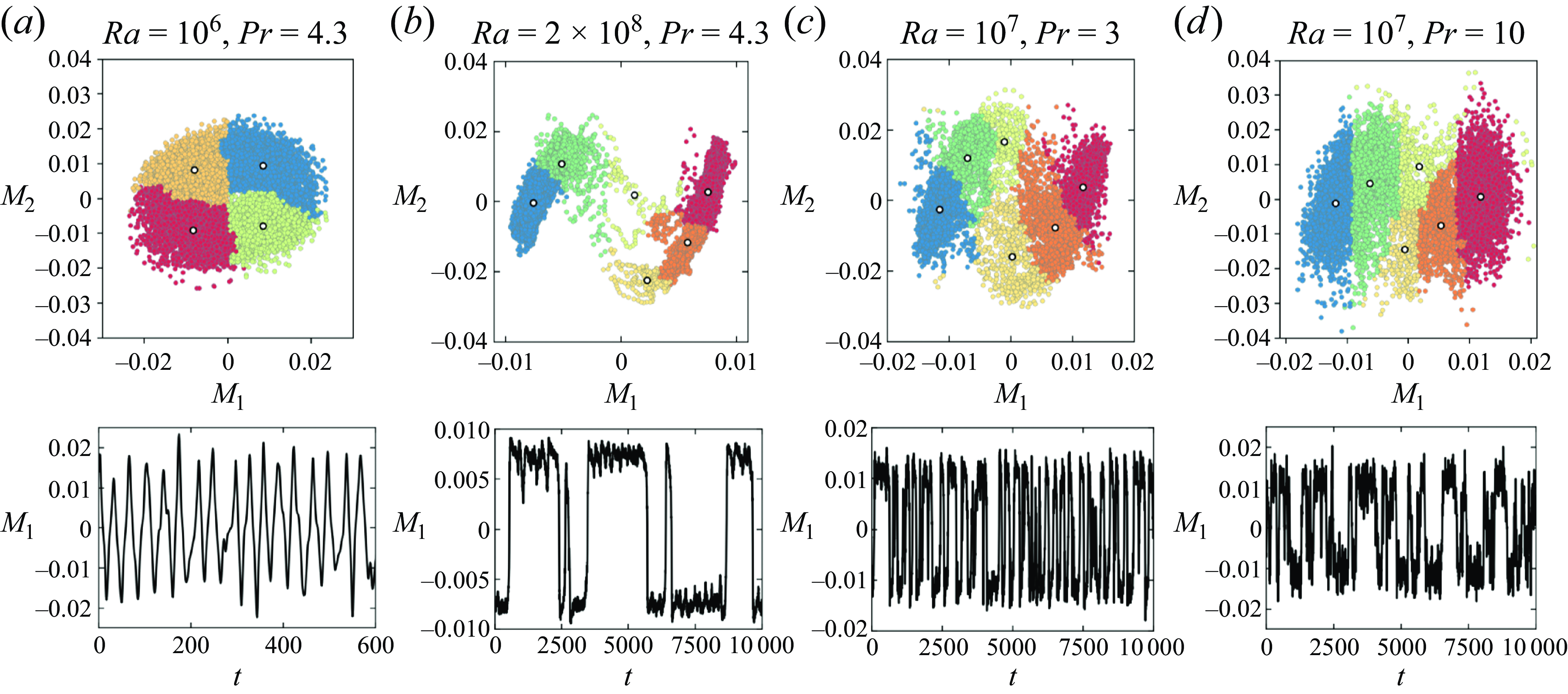
Figure 5. The two-dimensional phase space for different values of $Ra$
and
$Ra$
and $Pr$
, with the colours representing the communities identified based on (3.4), and the corresponding time series of the dominant mode
$Pr$
, with the colours representing the communities identified based on (3.4), and the corresponding time series of the dominant mode $M_1$
.
$M_1$
.
3.5.
Extension to different $Ra$
and
$Pr$
values
$Ra$
and
$Pr$
values


Finally, we extend our analysis to different values of $Ra$
and
$Ra$
and $Pr$
. The identified communities are shown in figure 5. From the cluster pattern, one can also gain insight into the dependence of flow reversals on
$Pr$
. The identified communities are shown in figure 5. From the cluster pattern, one can also gain insight into the dependence of flow reversals on $Ra$
and
$Ra$
and $Pr$
, in combination with the flow strength shown in figure 6. At low
$Pr$
, in combination with the flow strength shown in figure 6. At low $Ra$
, the flow reversal occurs periodically, and the cluster becomes well mixed without distinct branches; see figure 5(a). As
$Ra$
, the flow reversal occurs periodically, and the cluster becomes well mixed without distinct branches; see figure 5(a). As $Ra$
increases, the two stable regions increasingly separate, making transitions between the two different stable communities more difficult, as shown in figure 5(b). This separation continues until the Rayleigh number
$Ra$
increases, the two stable regions increasingly separate, making transitions between the two different stable communities more difficult, as shown in figure 5(b). This separation continues until the Rayleigh number $Ra$
exceeds a critical value (e.g.
$Ra$
exceeds a critical value (e.g. $Ra\gt 2\times 10^8$
at
$Ra\gt 2\times 10^8$
at $Pr=4.3$
), at which point the LSC is sufficiently strong (see the increasing flow strength as
$Pr=4.3$
), at which point the LSC is sufficiently strong (see the increasing flow strength as $Ra$
increases in figure 6) and flow reversals cease to occur. At both low and high Prandtl numbers
$Ra$
increases in figure 6) and flow reversals cease to occur. At both low and high Prandtl numbers $Pr$
, the two stable communities in the cluster pattern are not well separated, as shown in figures 5(c,d). This situation corresponds to a weaker LSC (see the flow strength in figure 6 at
$Pr$
, the two stable communities in the cluster pattern are not well separated, as shown in figures 5(c,d). This situation corresponds to a weaker LSC (see the flow strength in figure 6 at $Pr=10$
), which is due to chaotic plume emission that impedes the establishment of a stable LSC (Li et al. Reference Li, He, Tian, Hao and Huang2021). Consequently, flow reversals disappear at higher
$Pr=10$
), which is due to chaotic plume emission that impedes the establishment of a stable LSC (Li et al. Reference Li, He, Tian, Hao and Huang2021). Consequently, flow reversals disappear at higher $Ra$
due to a strong LSC, which suppresses the reversal, while they also diminish at low and high Prandtl numbers owing to a weak LSC.
$Ra$
due to a strong LSC, which suppresses the reversal, while they also diminish at low and high Prandtl numbers owing to a weak LSC.
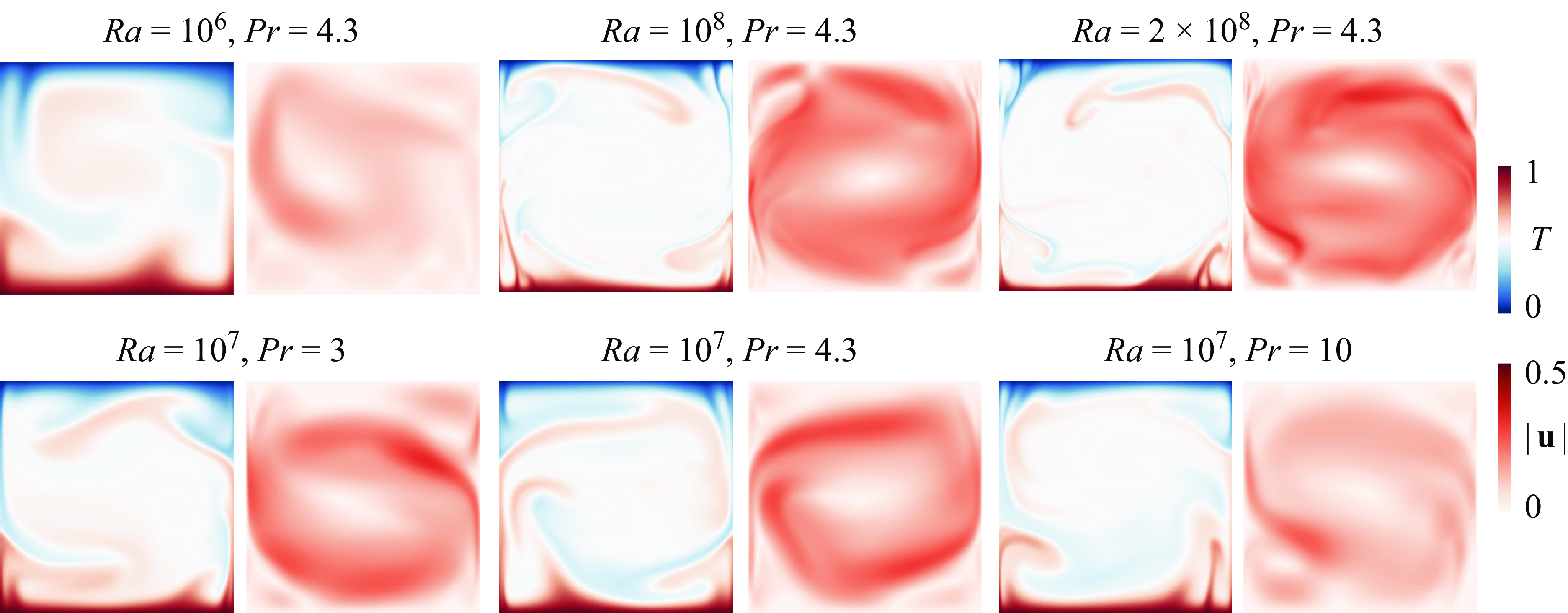
Figure 6. Snapshots of the temperature and flow strength fields for different $Ra$
and
$Ra$
and $Pr$
values.
$Pr$
values.
Note that the mode $M_1$
is always the first dominant mode, while
$M_1$
is always the first dominant mode, while $M_2$
is selected based on the cluster structures for different
$M_2$
is selected based on the cluster structures for different $Ra$
and
$Ra$
and $Pr$
, and the order may change due to the chaotic nature of the underlying flow; see more details in Appendix A. In previous work by Castillo-Castellanos et al. (Reference Castillo-Castellanos, Sergent, Podvin and Rossi2019), the cluster pattern was also explored for different
$Pr$
, and the order may change due to the chaotic nature of the underlying flow; see more details in Appendix A. In previous work by Castillo-Castellanos et al. (Reference Castillo-Castellanos, Sergent, Podvin and Rossi2019), the cluster pattern was also explored for different $Ra$
. While our cluster patterns differ from theirs due to a different selection of POD modes, the observed and reported tendency of cluster evolution with varying
$Ra$
. While our cluster patterns differ from theirs due to a different selection of POD modes, the observed and reported tendency of cluster evolution with varying $Ra$
shows similarities: for low
$Ra$
shows similarities: for low $Ra$
(
$Ra$
( $\sim 10^6$
), the cluster shrinks and is better mixed without a distinct branch, since the reversal becomes increasingly periodic, while for high
$\sim 10^6$
), the cluster shrinks and is better mixed without a distinct branch, since the reversal becomes increasingly periodic, while for high $Ra$
(
$Ra$
( $\gt 2\times 10^8$
), only one branch emerges as the reversal event disappears.
$\gt 2\times 10^8$
), only one branch emerges as the reversal event disappears.
4. Conclusions
In conclusion, we have presented a purely data-driven cluster-based approach utilizing set-theoretic tools and cluster analysis to examine reversal events in turbulent thermal convection. This method effectively represents the temporal evolution of the primary flow dynamics, including cluster identification and probability distributions for the system behaviour. The network-based model clearly identifies three types of key communities: the stable communities, where the large-scale circulation (LSC) maintains a consistent orientation; the transition communities, where the LSC is changing orientation, and the precursor community, where the LSC is stable but near transition, which is crucial for early prediction of reversal events. The cluster model is also capable of predicting flow reversals, using the cluster community information and the Markov matrix. We quantify the dependence of the prediction accuracy for the reversal events as a function of $\tau$
: for predictions later in the transition state, the results are very encouraging and accurate, whereas for predictions from the earlier stable state, we obtain results based on the ergodic probability. Additionally, the model’s cluster pattern offers insight into the mechanism of flow reversal within the
$\tau$
: for predictions later in the transition state, the results are very encouraging and accurate, whereas for predictions from the earlier stable state, we obtain results based on the ergodic probability. Additionally, the model’s cluster pattern offers insight into the mechanism of flow reversal within the $(Ra, Pr)$
parameter space. Specifically, reversals are suppressed at large Rayleigh numbers due to the presence of a strong LSC (represented by
$(Ra, Pr)$
parameter space. Specifically, reversals are suppressed at large Rayleigh numbers due to the presence of a strong LSC (represented by $M_1$
), reflected in the separation of stable communities in the cluster pattern. At high and low
$M_1$
), reflected in the separation of stable communities in the cluster pattern. At high and low $Pr$
and low
$Pr$
and low $Ra$
, on the other hand, the cluster pattern shows a mixing of states without distinct and well-separated communities due to chaotic plume emissions, and hence a weaker LSC.
$Ra$
, on the other hand, the cluster pattern shows a mixing of states without distinct and well-separated communities due to chaotic plume emissions, and hence a weaker LSC.
It is important to note that we use only two POD modes for the cluster analysis since they appear sufficient to capture the reversal event and angular momentum dynamics. Nevertheless, we emphasize that this cluster-based modelling framework can readily be applied to high-dimensional systems, as demonstrated in recent work (Giorgini, Souza & Schmid Reference Giorgini, Souza and Schmid2024); the cluster dynamics and reversal study in higher-dimensional systems deserves further exploration in a future effort.
Finally, this purely data-driven approach can be extended to other flow systems that switch between co-existing states or between persistent dynamics and rare events; examples, among many others, include bursts in zonal flows (von Hardenberg et al. Reference von Hardenberg, Goluskin, Provenzale and Spiegel2015), near-wall turbulence (Jiménez & Moin Reference Jiménez and Moin1991; Jiménez Reference Jiménez2023), buoyancy-driven phase-change flows (Yang et al. Reference Yang, Howland, Liu, Verzicco and Lohse2023; Du, Calzavarini & Sun Reference Du, Calzavarini and Sun2024), and pipe flows (Avila et al. Reference Avila, Barkley and Hof2023). Furthermore, potential applications in control-oriented extensions (Wang, Zhou & Sun Reference Wang, Zhou and Sun2020; Yang et al. Reference Yang, Chong, Wang, Verzicco, Shishkina and Lohse2020; Zhang et al. Reference Zhang, Xia, Zhou and Chen2020; Zhao et al. Reference Zhao, Wang, Wu, Chong and Zhou2022, Reference Zhao, Zhao, Zhou and Chong2024) could broaden its utility across various complex dynamical phenomena.
Supplementary movie
Supplementary movie is available at https://doi.org/10.1017/jfm.2025.371.
Acknowledgements
R.Y. would like to thank Professor D. Lohse and Professor A. Prosperetti for their helpful discussions and deep insights.
Funding
This research was supported by the 2022 Geophysical Fluid Dynamics Summer Fellowship at the Woods Hole Oceanographic Institution. R.Y. was also supported by the EuroHPC Joint Undertaking for awarding the projects EHPC-REG2022R03-208 and EHPC-REG-2023R03-178 for access to the EuroHPC supercomputer Discoverer. This work was also financially supported by the European Union (ERC, MultiMelt, 101094492).
Declaration of interests
The authors report no conflict of interest.
Appendix A. Proper orthogonal decomposition details
For high-dimensional data such as turbulent flow fields, data compression with lossless POD can reduce the computational cost of clustering by decomposing the data field $\textbf X$
into a set of POD modes according to
$\textbf X$
into a set of POD modes according to
 \begin{equation} X(n, t)=\sum _{k=1}^{\infty } a_k(t)\, \phi _k(n), \end{equation}
where $\phi _k(n)$
is a deterministic spatial function, and
$\phi _k(n)$
is a deterministic spatial function, and $a_k(t)$
is the corresponding temporal coefficient.
$a_k(t)$
is the corresponding temporal coefficient.
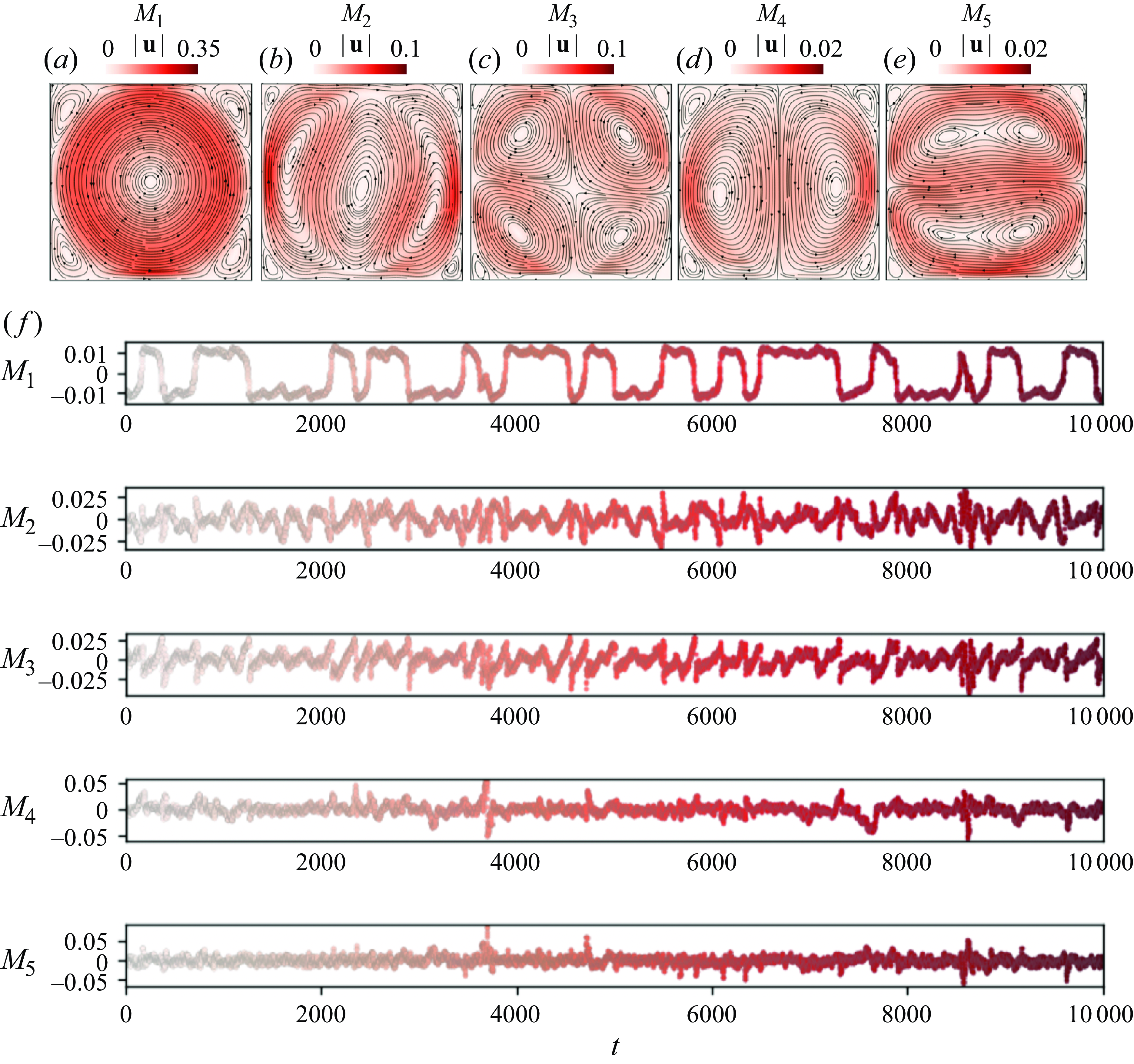
Figure 7. (a–e) The reconstructed velocity field, based on each of the first five POD modes for $Ra=10^8, Pr=4.3$
, with the colours representing the magnitude of the flow velocity, and the streamlines representing the direction of the flow. (f) The time series of the value of each POD mode.
$Ra=10^8, Pr=4.3$
, with the colours representing the magnitude of the flow velocity, and the streamlines representing the direction of the flow. (f) The time series of the value of each POD mode.
First, we reorganize the multidimensional data $(T, u_x, u_z)_{ij}$
in each snapshot into a corresponding one-dimensional real vector. At this stage we also downsample in space to further reduce the computational load (Yang et al. Reference Yang, Zhang, Reiter, Lohse, Shishkina and Linkmann2022). The time series can then be represented by an ordered sequence
$(T, u_x, u_z)_{ij}$
in each snapshot into a corresponding one-dimensional real vector. At this stage we also downsample in space to further reduce the computational load (Yang et al. Reference Yang, Zhang, Reiter, Lohse, Shishkina and Linkmann2022). The time series can then be represented by an ordered sequence ${\textbf X}={\textbf x}_{n},\ n=1,\ldots, N$
, where
${\textbf X}={\textbf x}_{n},\ n=1,\ldots, N$
, where $N$
represents the number of snapshots. We next decompose
$N$
represents the number of snapshots. We next decompose $\textbf X$
using a singular value decomposition according to
$\textbf X$
using a singular value decomposition according to ${\textbf X}={\textbf U} \Sigma {\textbf V}^{*}$
, where
${\textbf X}={\textbf U} \Sigma {\textbf V}^{*}$
, where $\textbf U$
contains the spatial structures
$\textbf U$
contains the spatial structures $\phi _k(n)$
,
$\phi _k(n)$
, $\Sigma$
contains the magnitudes of each mode, and
$\Sigma$
contains the magnitudes of each mode, and ${\textbf V}^{*}$
contains the temporal coefficients
${\textbf V}^{*}$
contains the temporal coefficients $a_k(t)$
.
$a_k(t)$
.
For example, the reconstructed flow structures based on each of the first five POD modes for $Ra=10^8,\ Pr=4.3$
are shown in figure 7. Each of them shows a characteristic flow pattern, related to the LSC. In figure 8, we display the two-dimensional phase spaces of different combinations of POD modes; from this figure, we conclude that only the
$Ra=10^8,\ Pr=4.3$
are shown in figure 7. Each of them shows a characteristic flow pattern, related to the LSC. In figure 8, we display the two-dimensional phase spaces of different combinations of POD modes; from this figure, we conclude that only the $(M_1, M_2)$
phase space captures both stable states as well as distinct transition states. The dominant modes are similar to those reported in Podvin & Sergent (Reference Podvin and Sergent2015), albeit in different order – a feature attributable to a different
$(M_1, M_2)$
phase space captures both stable states as well as distinct transition states. The dominant modes are similar to those reported in Podvin & Sergent (Reference Podvin and Sergent2015), albeit in different order – a feature attributable to a different $Ra$
or the chaotic nature of the underlying flow.
$Ra$
or the chaotic nature of the underlying flow.
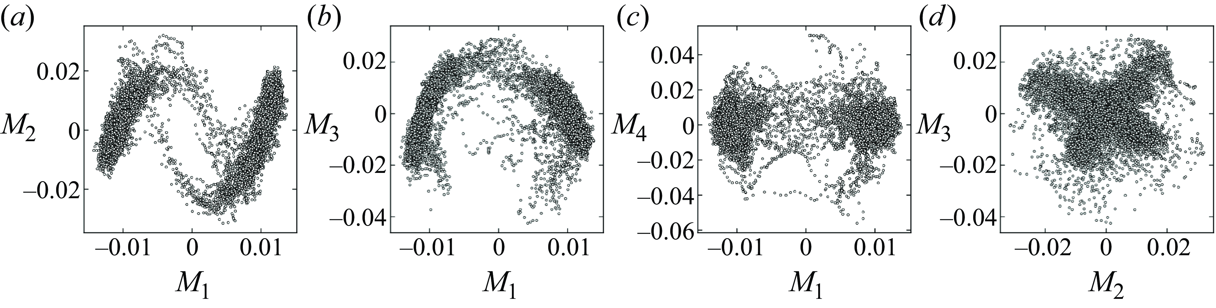
Figure 8. Two-dimensional phase spaces of (a) $(M_1, M_2)$
, (b)
$(M_1, M_2)$
, (b) $(M_1, M_3)$
, (c)
$(M_1, M_3)$
, (c) $(M_1, M_4)$
, (d)
$(M_1, M_4)$
, (d) $(M_2, M_3)$
.
$(M_2, M_3)$
.
Appendix B. The discretization resolution effect on the cluster modelling
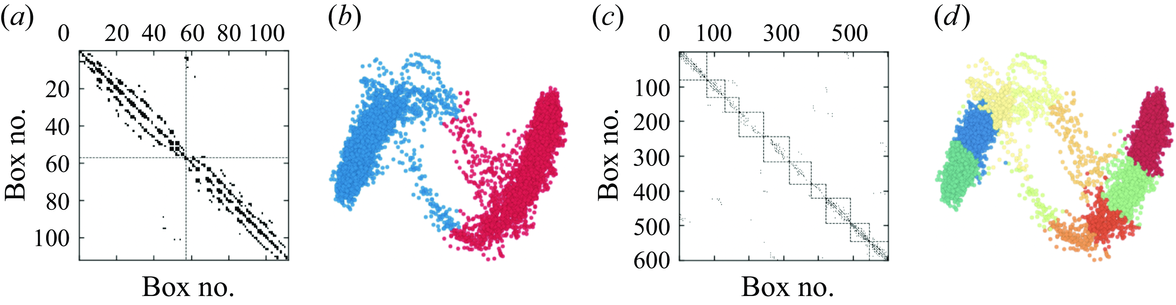
Figure 9. (a) Fill pattern of the transition probability matrix after the clustering algorithm with box number 15 in both directions, consisting of 112 cells in total, and displaying two communities. (b) The corresponding phase space of $M_1$
and
$M_1$
and $M_2$
, with the colours representing different clusters. (c) Fill pattern of the transition probability matrix after the clustering algorithm with box number 40 in both directions, consisting of 601 cells in total, and displaying ten communities. (d) The corresponding phase space of
$M_2$
, with the colours representing different clusters. (c) Fill pattern of the transition probability matrix after the clustering algorithm with box number 40 in both directions, consisting of 601 cells in total, and displaying ten communities. (d) The corresponding phase space of $M_1$
and
$M_1$
and $M_2$
, with the colours representing different clusters.
$M_2$
, with the colours representing different clusters.
The discretization of phase space is marked by crucial adjustable parameters in our analysis. It must be sufficiently fine to accurately approximate the phase-space trajectory, and at the same time sufficiently coarse to contain enough trajectory points for a precise representation of the transition probabilities. To demonstrate the impact of the discretization box size, we compare results using 15 boxes in both directions (low resolution), and 40 boxes in both directions (high resolution). As shown in figure 9, a low-resolution discretization (figures 9 a,b) leads to the clusters being divided into two communities, losing detailed information about the precursor and transition regions. Conversely, a high-resolution discretization (figures 9 c,d) identifies more independent communities, providing detailed information about the transition regions.
Although higher resolutions may lead to a more discerning subdivision of stable, transition and precursor communities, the overall flow structures within these sub-communities remain consistent. If one can reliably identify the main flow structures and associate the sub-communities with stable, transition or precursor states, then the full model would still be effective. For clarity and conciseness, we have chosen an intermediate resolution of $25$
boxes in this work; this resolution allows us to distinguish the stable, precursor and transition regions, without introducing redundant information from too many clusters.
$25$
boxes in this work; this resolution allows us to distinguish the stable, precursor and transition regions, without introducing redundant information from too many clusters.
Appendix C. Comparison with the
$K$
-means clustering method

The $K$
-means clustering method is an unsupervised machine learning algorithm, which is widely used to group unlabelled datasets into different clusters (Brunton & Kutz Reference Brunton and Kutz2022). It has also been applied in previous studies of fluid flows (Kaiser et al. Reference Kaiser2014; Castillo-Castellanos et al. Reference Castillo-Castellanos, Sergent, Podvin and Rossi2019; Fernex et al. Reference Fernex, Noack and Semaan2021; Hou et al. Reference Hou, Deng and Noack2024). In this appendix, we include a comparison of our method to
$K$
-means clustering method is an unsupervised machine learning algorithm, which is widely used to group unlabelled datasets into different clusters (Brunton & Kutz Reference Brunton and Kutz2022). It has also been applied in previous studies of fluid flows (Kaiser et al. Reference Kaiser2014; Castillo-Castellanos et al. Reference Castillo-Castellanos, Sergent, Podvin and Rossi2019; Fernex et al. Reference Fernex, Noack and Semaan2021; Hou et al. Reference Hou, Deng and Noack2024). In this appendix, we include a comparison of our method to $K$
-means clustering for the phase space of our reversal dynamics, shown in figure 10.
$K$
-means clustering for the phase space of our reversal dynamics, shown in figure 10.
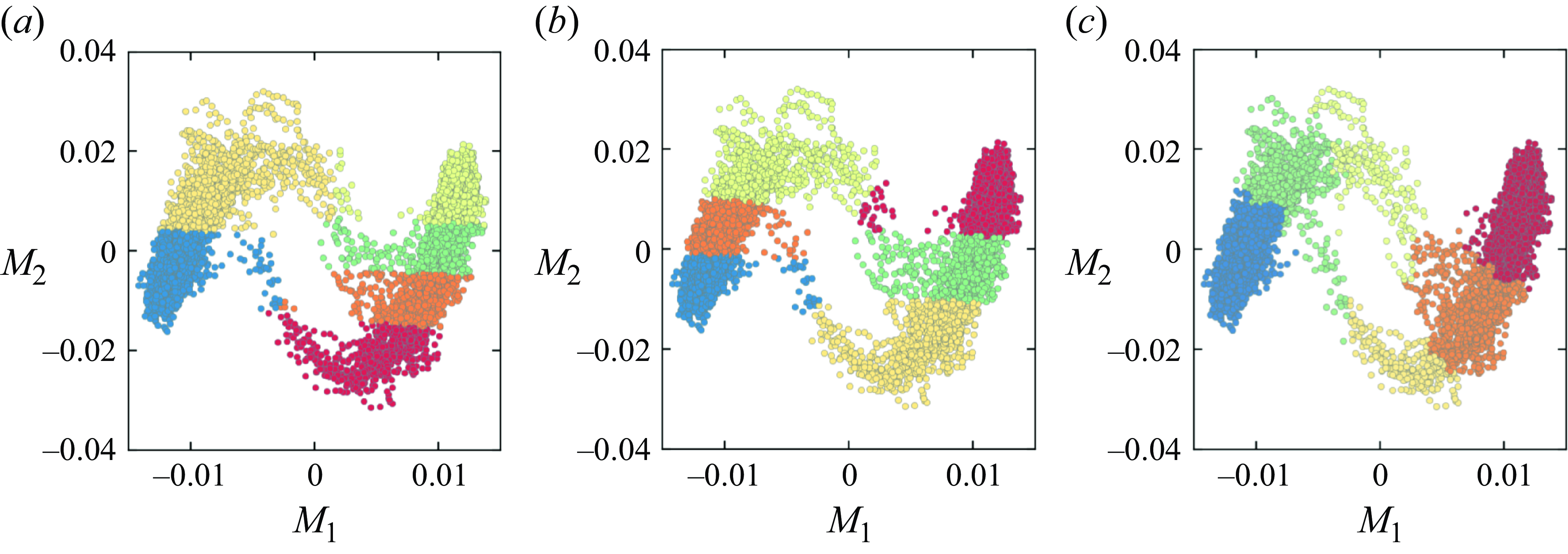
Figure 10. The results of clustering of the $(M_1,M_2)$
phase space using (a,b) the
$(M_1,M_2)$
phase space using (a,b) the $K$
-means algorithm with different random initializations of the centroids, and (c) our method.
$K$
-means algorithm with different random initializations of the centroids, and (c) our method.
The results confirm the sensitivity of the $K$
-means algorithm to the random initialization of the centroids (see figures 10
a,b), combined with a convergence towards a local minimum. Even in the case when the
$K$
-means algorithm to the random initialization of the centroids (see figures 10
a,b), combined with a convergence towards a local minimum. Even in the case when the $K$
-means algorithm produces acceptable and symmetric results (figure 10
b), an obvious mixing of stable and transition communities persists. This shortcoming emerges since the
$K$
-means algorithm produces acceptable and symmetric results (figure 10
b), an obvious mixing of stable and transition communities persists. This shortcoming emerges since the $K$
-means algorithm takes into account only the spatial distribution of data points, ignoring directional information in the network’s connectivity pattern.
$K$
-means algorithm takes into account only the spatial distribution of data points, ignoring directional information in the network’s connectivity pattern.
Appendix D. Comparison with a simple threshold-based correction scheme for predicting reversal
In this appendix, we compare the prediction of reversals from our model to predictions from a simple threshold-based approach that uses an arbitrary value of $|L|$
. For the threshold-based method, we predict flow reversals based on the condition
$|L|$
. For the threshold-based method, we predict flow reversals based on the condition $(|L(t)|-L_{c})(|L(t+1)|-L_{c})\lt 0$
, where
$(|L(t)|-L_{c})(|L(t+1)|-L_{c})\lt 0$
, where $L_c$
denotes a threshold for the reversal, combined with the sign of the gradient of
$L_c$
denotes a threshold for the reversal, combined with the sign of the gradient of $L(t)$
. The results of the comparison are presented in figure 11. We observe that the accuracy of the latter method is limited by the presence of natural fluctuations in the
$L(t)$
. The results of the comparison are presented in figure 11. We observe that the accuracy of the latter method is limited by the presence of natural fluctuations in the $|L|$
curve. These fluctuations often lead to false predictions or missed transitions, especially in cases where
$|L|$
curve. These fluctuations often lead to false predictions or missed transitions, especially in cases where $|L|$
exhibits declines that do not correspond to actual reversals. In contrast, our model uses cluster information to effectively filter out most of these fluctuations, enabling it to produce more robust and systematic predictions without the need for additional constraints.
$|L|$
exhibits declines that do not correspond to actual reversals. In contrast, our model uses cluster information to effectively filter out most of these fluctuations, enabling it to produce more robust and systematic predictions without the need for additional constraints.
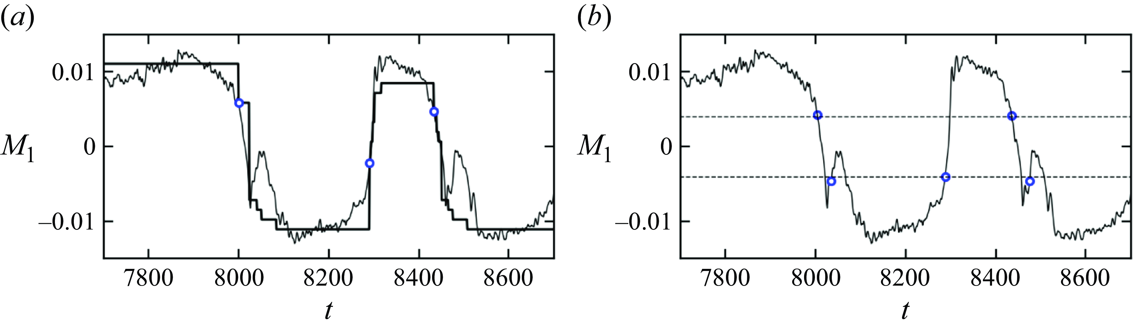
Figure 11. (a) The prediction of reversals based on our cluster-based method. The blue points represent the predicted reversal locations. (b) The prediction of the reversal based on the simple threshold-based method. The blue points represent the predicted reversal locations. The dashed lines show the value of the threshold, which we adjusted to a value similar to that in our model.
Hence a key advantage of our approach lies in its ability to handle fluctuations without requiring special constraints, which in turn yields a robust and effective framework for reversal prediction. Despite this advantage, it remains challenging to achieve accurate predictions in the earlier states due to the chaotic nature of the system. We acknowledge this limitation, and plan to investigate further improvements in this direction.


 Open access