


1 Introduction
Gravity currents are primarily horizontal flows driven by gravity acting on the density difference between fluids. In porous media, gravity currents describe the behaviour of flows relevant to geological carbon sequestration, geothermal energy, groundwater flows and the motion of contaminants in the subsurface, for example. The behaviour of gravity currents in porous media has been studied extensively, both experimentally and theoretically. The majority of these studies consider long, thin currents, propagating through homogeneous porous media with no mixing between the fluids. However, due to the complexity of flow within realistic geological media, the distribution of fluids may become dispersed by heterogeneities at a range of scales and hence the behaviour of these buoyancy-driven flows may differ significantly from idealized models. It is therefore important to incorporate the mixing between fluids driven by the complexity of the pore space and natural heterogeneities within the rocks in models of gravity currents in porous media.
Unconfined gravity currents in porous media have been studied theoretically and experimentally by Huppert & Woods (Reference Huppert and Woods1995) for rectilinear geometries and by Lyle et al. (Reference Lyle, Huppert, Hallworth, Bickle and Chadwick2005) for the axisymmetric case. These models are based on the assumption that (i) the gravity currents are long and thin so that the vertical velocity can be neglected, (ii) the background flow is negligible when the ambient is much deeper than the current and (iii) that there is no mixing between the injected and ambient fluids, commonly referred to as the sharp-interface assumption. In both geometries the gravity currents exhibit a self-similar behaviour as described previously by Pattle (Reference Pattle1959). The propagation of gravity currents in porous media has been studied further with additional geometrical complications. For example, gravity currents on an inclined surface have been studied by Vella & Huppert (Reference Vella and Huppert2006) and Gunn & Woods (Reference Gunn and Woods2011), or in a vertically confined medium by Nordbotten, Celia & Bachu (Reference Nordbotten, Celia and Bachu2005), MacMinn et al. (Reference MacMinn, Neufeld, Hesse and Huppert2012), Pegler, Huppert & Neufeld (Reference Pegler, Huppert and Neufeld2014) and Zheng et al. (Reference Zheng, Guo, Christov, Celia and Stone2015). Moreover, by relaxing the restriction of a homogeneous medium, Pritchard, Woods & Hogg (Reference Pritchard, Woods and Hogg2001), Goda & Sato (Reference Goda and Sato2011) and Sahu & Flynn (Reference Sahu and Flynn2017) have investigated gravity currents in layered porous media of differing permeabilities, while Zheng, Christov & Stone (Reference Zheng, Christov and Stone2014) have investigated flow in horizontally heterogeneous medium. Formulations for modelling gravity currents in a highly heterogeneous medium have been presented by Anderson, McLaughlin & Miller (Reference Anderson, McLaughlin and Miller2003, Reference Anderson, McLaughlin and Miller2004), who describe homogenization methods for the averaging of medium properties. Apart from considering various geometries, the effects of non-uniform fluid properties in porous gravity currents have also been investigated. Some examples include: two-layer or stratified gravity currents by Woods & Mason (Reference Woods and Mason2000) and Pegler, Huppert & Neufeld (Reference Pegler, Huppert and Neufeld2016), respectively; vaporizing gravity currents by Woods & Mason (Reference Woods and Mason1998); and non-Newtonian gravity currents in porous media by Ciriello et al. (Reference Ciriello, Longo, Chiapponi and Di Federico2016) and Lauriola et al. (Reference Lauriola, Felisa, Petrolo, Di Federico and Longo2018).
For miscible fluids in porous medium, mass transfer of solute occurs either by molecular diffusion if the system is static, or by hydrodynamic dispersion if there is flow (Delgado Reference Delgado2007; Woods Reference Woods2015). However, the effects of mixing between the gravity current and ambient fluid remain largely unexplored despite the extensive literature on porous medium gravity currents outlined above. Some examples, where mass transfer across the interface during a density-driven flow have been explored, include convective dissolution which occurs during geological carbon sequestration (Neufeld et al. Reference Neufeld, Hesse, Riaz, Hallworth, Tchelepi and Huppert2010; MacMinn et al. Reference MacMinn, Neufeld, Hesse and Huppert2012; Guo et al. Reference Guo, Bandilla, Nordbotten, Celia, Keilegavlen and Doster2016) and the intrusion of sea water into coastal aquifers (Huyakorn et al. Reference Huyakorn, Andersen, Mercer and White1987; Dentz et al. Reference Dentz, Tartakovsky, Abarca, Guadagnini, Sanchez-Vila and Carrera2006; Pastar & Dagan Reference Pastar and Dagan2007). Solute transport obeys a Fickian model of dispersion when the medium is homogeneous. However, given the heterogeneous nature of aquifers, mixing of solute with the ambient generally occurs in a non-Fickian regime. A significant amount of work has been done on modelling solute transport in heterogeneous, three-dimensional media using stochastic methods, which have proved to be a helpful tool in capturing the anomalies in solute transport in more realistic field problems (Carrera Reference Carrera1993; Fleurant & van der Lee Reference Fleurant and van der Lee2001; Verwoerd Reference Verwoerd2007; Fiori et al. Reference Fiori, Bellin, Cvetkovic, de Barros and Dagan2015).
An investigation of mixing in miscible gravity currents that more directly addresses mixing between fluids is the work of Szulczewski & Juanes (Reference Szulczewski and Juanes2013). In that study the authors considered mixing due to molecular diffusion between dense and light fluids within a confined porous layer. They investigated the case of a constant volume release and found the time-dependent evolution of the interface and concentration. They identify five regimes: early diffusion, S slumping, straight-line slumping, Taylor slumping and late diffusion. They find that diffusion is predominant in the early and late-time regimes, whereas in the S-slumping and straight-line-slumping regimes the interface remains sharp. However, in the Taylor-slumping regime, they show that the mixing is enhanced through Taylor dispersion. Their study, however, did not consider the effects of enhanced mixing through dispersion driven by the flow. It may be anticipated that at early and late times, where the velocity is small, mixing is diffusive, but that at intermediate times mixing is enhanced through dispersion. Furthermore, it may be anticipated that the mixing in the unconfined limit may differ substantially from that found in confined aquifers.
The prevalence of dispersion in miscible gravity currents is apparent in previous work, for example in flows through homogeneous porous media by Sahu & Flynn (Reference Sahu and Flynn2015) and Pegler et al. (Reference Pegler, Maskell, Daniels and Bickle2017) – see their figures 6 and 12, respectively, and the associated discussions. In multilayered porous media this mixing may be greatly enhanced as observed in the laboratory experiments of Huppert, Neufeld & Strandkvist (Reference Huppert, Neufeld and Strandkvist2013, figure 7) and Sahu & Flynn (Reference Sahu and Flynn2015, figure 4). In those studies the volume of the current became larger than that anticipated by the fluid injected alone. In practice, most geological aquifers are highly heterogeneous (Alpay Reference Alpay1972) and the fluids are not entirely immiscible (Enick & Klara Reference Enick and Klara1990), so it may be anticipated that the effects of mixing during flow may be significant.
In this paper we present a model of mixing in porous medium gravity currents, considering mechanical dispersion as the primary source of entrainment. We consider the case of a continuous, constant volume flux injection and begin by presenting a general mathematical model for dispersive entrainment in gravity currents in porous media in § 2. In § 3 we demonstrate the character of the flow and mixing through mathematical analysis. In § 4 we present laboratory exteriments and explain how we determine the concentration and hence mixing rates from laboratory images. In § 4.3 we present a comparison between the mathematical model and our experimental results. In § 5 we compare the findings from the current model with the previous models and also describe how the current entrainment model may be applied more broadly to heterogeneous porous media. Finally, in § 6 we conclude by summarizing the current work and identifying future problems of interest.
2 Mathematical model of flow and dispersive entrainment
2.1 Governing equations
We consider the injection of a fluid of initial concentration $C_{0}$
, and hence density
$C_{0}$
, and hence density $\unicode[STIX]{x1D70C}_{0}$
, at fixed volume flux
$\unicode[STIX]{x1D70C}_{0}$
, at fixed volume flux $q$
into a large, horizontal porous medium of uniform porosity
$q$
into a large, horizontal porous medium of uniform porosity $\unicode[STIX]{x1D719}$
and permeability
$\unicode[STIX]{x1D719}$
and permeability $k$
that is initially saturated with an ambient fluid of concentration
$k$
that is initially saturated with an ambient fluid of concentration $C_{a}=0$
and density
$C_{a}=0$
and density $\unicode[STIX]{x1D70C}_{a}$
. In general, flow through the porous medium is described by a statement of mass conservation, Darcy’s law, a statement of conservation of solute as expressed by an advection–diffusion relationship, and an equation of state describing the dependence of the density on concentration,
$\unicode[STIX]{x1D70C}_{a}$
. In general, flow through the porous medium is described by a statement of mass conservation, Darcy’s law, a statement of conservation of solute as expressed by an advection–diffusion relationship, and an equation of state describing the dependence of the density on concentration,
 $$\begin{eqnarray}\displaystyle & \displaystyle \unicode[STIX]{x1D735}\boldsymbol{\cdot }\boldsymbol{u}=0, & \displaystyle\end{eqnarray}$$
 $$\begin{eqnarray}\displaystyle & \displaystyle \boldsymbol{u}=-\frac{k}{\unicode[STIX]{x1D707}}(\unicode[STIX]{x1D735}p+\unicode[STIX]{x1D70C}g\hat{\boldsymbol{z}}), & \displaystyle\end{eqnarray}$$
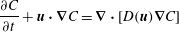 $$\begin{eqnarray}\displaystyle & \displaystyle \frac{\unicode[STIX]{x2202}C}{\unicode[STIX]{x2202}t}+\boldsymbol{u}\boldsymbol{\cdot }\unicode[STIX]{x1D735}C=\unicode[STIX]{x1D735}\boldsymbol{\cdot }[D(\boldsymbol{u})\unicode[STIX]{x1D735}C] & \displaystyle\end{eqnarray}$$
 $$\begin{eqnarray}\displaystyle & \displaystyle \unicode[STIX]{x1D70C}(\boldsymbol{x},t)=\unicode[STIX]{x1D70C}_{a}[1+\unicode[STIX]{x1D6FD}(C(\boldsymbol{x},t)-C_{a})]. & \displaystyle\end{eqnarray}$$
Here, $\unicode[STIX]{x1D707}$
is the dynamic viscosity,
$\unicode[STIX]{x1D707}$
is the dynamic viscosity, $p$
is pressure,
$p$
is pressure, $\boldsymbol{x}=(x,z)$
represents the horizontal and vertical coordinates,
$\boldsymbol{x}=(x,z)$
represents the horizontal and vertical coordinates, $\boldsymbol{u}=(u,w)$
is the velocity vector and
$\boldsymbol{u}=(u,w)$
is the velocity vector and $D(\boldsymbol{u})$
is, in general, the dispersion coefficient of concentration and
$D(\boldsymbol{u})$
is, in general, the dispersion coefficient of concentration and $\unicode[STIX]{x1D6FD}$
is the coefficient of solute contraction.
$\unicode[STIX]{x1D6FD}$
is the coefficient of solute contraction.
This general model for buoyancy-driven flow presents a challenge for numerical simulations over very large lateral length scales. Our aim is therefore to construct a reduced model of the average properties within the current using parameterizations, where appropriate, of the vertical structure. We focus on cases where the depth of the medium is large, and hence the flow of the ambient fluid may be neglected (the so-called unconfined limit). Further, we consider cases where the lateral extent of the current is much greater than the vertical extent. In this limit, scaling analysis of (2.1)–(2.3) suggests that for long, thin currents $|w|\ll |u|$
and the pressure is hydrostatic
$|w|\ll |u|$
and the pressure is hydrostatic
 $$\begin{eqnarray}p(x,z,t)=p_{H}+\unicode[STIX]{x1D70C}_{a}g(H-z)+\unicode[STIX]{x1D70C}_{a}g\unicode[STIX]{x1D6FD}\int _{z}^{h}[C(x,z,t)-C_{a}]\,\text{d}z,\quad (0\leqslant z\leqslant h).\end{eqnarray}$$
Here, $w$
and
$w$
and $u$
are the vertical and horizontal velocities of the current and
$u$
are the vertical and horizontal velocities of the current and $h(x,t)$
is the gravity current height, which is identified as the interface between the current and ambient where
$h(x,t)$
is the gravity current height, which is identified as the interface between the current and ambient where $C(x,z=h,t)\approx C_{a}$
, and
$C(x,z=h,t)\approx C_{a}$
, and $p_{H}$
is the pressure at a reference height
$p_{H}$
is the pressure at a reference height $z=H\gg h$
. Since the pressure is hydrostatic the horizontal velocity of the current is
$z=H\gg h$
. Since the pressure is hydrostatic the horizontal velocity of the current is
 $$\begin{eqnarray}u=-\frac{k}{\unicode[STIX]{x1D707}}\frac{\unicode[STIX]{x2202}p}{\unicode[STIX]{x2202}x}=-\frac{k\unicode[STIX]{x1D70C}_{a}g\unicode[STIX]{x1D6FD}}{\unicode[STIX]{x1D707}}\left[\frac{\unicode[STIX]{x2202}}{\unicode[STIX]{x2202}x}\int _{0}^{h}(C-C_{a})\,\text{d}z\right]\simeq -\frac{k\unicode[STIX]{x1D70C}_{a}g\unicode[STIX]{x1D6FD}}{\unicode[STIX]{x1D707}}\frac{\unicode[STIX]{x2202}[h(\overline{C}-C_{a})]}{\unicode[STIX]{x2202}x},\end{eqnarray}$$
where the depth-averaged concentration
 $$\begin{eqnarray}\overline{C}(x,t)=C_{a}+\frac{1}{h}\int _{0}^{h}[C(x,z,t)-C_{a}]\,\text{d}z.\end{eqnarray}$$
Here, we make an ansatz that the concentration within the current is uniform with depth, and only varies over a mixing region of width $\unicode[STIX]{x1D6FF}$
at
$\unicode[STIX]{x1D6FF}$
at $z=h$
. This assumption may be generalized to a self-symmetric concentration profile throughout the length of the current – see for example Johnson & Hogg (Reference Johnson and Hogg2013). In effect, we neglect vertical variations in the concentration throughout the current, except at the edge as depicted in figure 1, and model only the evolution of the bulk concentration.
$z=h$
. This assumption may be generalized to a self-symmetric concentration profile throughout the length of the current – see for example Johnson & Hogg (Reference Johnson and Hogg2013). In effect, we neglect vertical variations in the concentration throughout the current, except at the edge as depicted in figure 1, and model only the evolution of the bulk concentration.

Figure 1. Schematic of a gravity current in a porous medium indicating how dispersion may be incorporated through an effective entrainment. The red curve depicts a typical vertical concentration profile throughout the current.
Considering that mass transfer due to concentration gradient occurs at the gravity current edge through dispersion, the flux of concentration through $z=h$
must be zero so that a kinematic condition describing the surface of the current may be written as
$z=h$
must be zero so that a kinematic condition describing the surface of the current may be written as
 $$\begin{eqnarray}\unicode[STIX]{x1D719}C|_{h}\frac{\unicode[STIX]{x2202}h}{\unicode[STIX]{x2202}t}+(uC)|_{h}\frac{\unicode[STIX]{x2202}h}{\unicode[STIX]{x2202}x}=(wC)|_{h}-\left.D\frac{\unicode[STIX]{x2202}C}{\unicode[STIX]{x2202}z}\right|_{h}.\end{eqnarray}$$
It is worth emphasizing that, as defined by the concentration contour $C(h,t)$
, growth of the current may be driven by both advection and diffusive or dispersive mixing. The evolution of the bulk concentration is therefore constrained by a depth integral of (2.3) along with the kinematic condition (2.8) and the velocity model (2.6),
$C(h,t)$
, growth of the current may be driven by both advection and diffusive or dispersive mixing. The evolution of the bulk concentration is therefore constrained by a depth integral of (2.3) along with the kinematic condition (2.8) and the velocity model (2.6),
 $$\begin{eqnarray}\unicode[STIX]{x1D719}\frac{\unicode[STIX]{x2202}(h\overline{C})}{\unicode[STIX]{x2202}t}-\frac{k\unicode[STIX]{x1D70C}_{a}g\unicode[STIX]{x1D6FD}}{\unicode[STIX]{x1D707}}\frac{\unicode[STIX]{x2202}}{\unicode[STIX]{x2202}x}\left[h\overline{C}\frac{\unicode[STIX]{x2202}(h\overline{C})}{\unicode[STIX]{x2202}x}\right]=0.\end{eqnarray}$$
This equation expresses conservation of solute, or buoyancy, within the current. Depth integration of a statement of conservation of mass, equation (2.1), along with the kinematic condition
 $$\begin{eqnarray}\unicode[STIX]{x1D719}\frac{\unicode[STIX]{x2202}h}{\unicode[STIX]{x2202}t}+u\frac{\unicode[STIX]{x2202}h}{\unicode[STIX]{x2202}x}=w+\frac{D}{\overline{C}-C_{a}}\left.\frac{\unicode[STIX]{x2202}C}{\unicode[STIX]{x2202}z}\right|_{h},\end{eqnarray}$$
provides a second equation that expresses conservation of mass within the current
 $$\begin{eqnarray}\unicode[STIX]{x1D719}\frac{\unicode[STIX]{x2202}h}{\unicode[STIX]{x2202}t}-\frac{k\unicode[STIX]{x1D70C}_{a}g\unicode[STIX]{x1D6FD}}{\unicode[STIX]{x1D707}}\frac{\unicode[STIX]{x2202}}{\unicode[STIX]{x2202}x}\left(h\frac{\unicode[STIX]{x2202}(h\overline{C})}{\unicode[STIX]{x2202}x}\right)=\frac{D}{\overline{C}-C_{a}}\left.\frac{\unicode[STIX]{x2202}C}{\unicode[STIX]{x2202}z}\right|_{h}=w_{e}.\end{eqnarray}$$
Here, mixing across the concentration boundary layer at the edge of the current is modelled by an effective diffusive or dispersive entrainment $w_{e}$
. For dispersive processes, we therefore approximate the effective entrainment of ambient fluid over a small length scale
$w_{e}$
. For dispersive processes, we therefore approximate the effective entrainment of ambient fluid over a small length scale $\unicode[STIX]{x1D6FF}$
to be
$\unicode[STIX]{x1D6FF}$
to be
 $$\begin{eqnarray}w_{e}\simeq \frac{D_{m}+\tilde{\unicode[STIX]{x1D6FC}}u}{\unicode[STIX]{x1D6FF}}\simeq \unicode[STIX]{x1D6FC}u\end{eqnarray}$$
for processes in which Péclet number,
 $$\begin{eqnarray}Pe=\tilde{\unicode[STIX]{x1D6FC}}u/D_{m}\gg 1,\end{eqnarray}$$
such that dispersion dominates (Delgado Reference Delgado2007; Woods Reference Woods2015). Here $D_{m}$
is the molecular diffusivity,
$D_{m}$
is the molecular diffusivity, $\unicode[STIX]{x1D6FC}=\tilde{\unicode[STIX]{x1D6FC}}/\unicode[STIX]{x1D6FF}\sim O(1)$
is the effective entrainment coefficient and
$\unicode[STIX]{x1D6FC}=\tilde{\unicode[STIX]{x1D6FC}}/\unicode[STIX]{x1D6FF}\sim O(1)$
is the effective entrainment coefficient and $\tilde{\unicode[STIX]{x1D6FC}}$
and
$\tilde{\unicode[STIX]{x1D6FC}}$
and $\unicode[STIX]{x1D6FF}$
are representative of the pore scale. This dimensionless transverse dispersivity plays a role that is qualitatively similar to the entrainment coefficient in turbulent plumes and gravity currents (Morton, Taylor & Turner Reference Morton, Taylor and Turner1956; Johnson & Hogg Reference Johnson and Hogg2013). Here, for simplicity, we assume that the non-dimensional transverse dispersivity
$\unicode[STIX]{x1D6FF}$
are representative of the pore scale. This dimensionless transverse dispersivity plays a role that is qualitatively similar to the entrainment coefficient in turbulent plumes and gravity currents (Morton, Taylor & Turner Reference Morton, Taylor and Turner1956; Johnson & Hogg Reference Johnson and Hogg2013). Here, for simplicity, we assume that the non-dimensional transverse dispersivity $\unicode[STIX]{x1D6FC}\approx$
constant, and constrain the value of this entrainment constant through experimental measurements in § 4.3. It is important to note that we neglect the longitudinal, or horizontal, entrainment in our model and leave its inclusion for a future study.
$\unicode[STIX]{x1D6FC}\approx$
constant, and constrain the value of this entrainment constant through experimental measurements in § 4.3. It is important to note that we neglect the longitudinal, or horizontal, entrainment in our model and leave its inclusion for a future study.
Equations (2.9) and (2.11) express the local conservation of buoyancy and mass respectively. At the origin, $x=0$
, mass and concentration are injected at rates
$x=0$
, mass and concentration are injected at rates
 $$\begin{eqnarray}\displaystyle q=[uh]_{x=0},\quad \text{and}\quad q(C_{0}-C_{a})=[u(\overline{C}-C_{a})h]_{x=0}, & & \displaystyle\end{eqnarray}$$
respectively, where $q$
is the volume flux into the current and
$q$
is the volume flux into the current and $C_{0}$
the initial concentration. Note that (2.14a,b
) can be used to show that the concentration at the origin is fixed at the input concentration,
$C_{0}$
the initial concentration. Note that (2.14a,b
) can be used to show that the concentration at the origin is fixed at the input concentration,
 $$\begin{eqnarray}\overline{C}(0,t)=C_{0}.\end{eqnarray}$$
Globally, concentration, or equivalently buoyancy, is conserved within the current
 $$\begin{eqnarray}qt(C_{0}-C_{a})=\unicode[STIX]{x1D719}\int _{0}^{x_{N}}(\overline{C}-C_{a})h\,\text{d}x,\end{eqnarray}$$
where $x_{N}(t)$
is the extent of the gravity current. Equation (2.16) together with (2.14) and (2.9) imply that there is no buoyancy flux through the nose of the current,
$x_{N}(t)$
is the extent of the gravity current. Equation (2.16) together with (2.14) and (2.9) imply that there is no buoyancy flux through the nose of the current,
 $$\begin{eqnarray}[u(\overline{C}-C_{a})h]_{x_{N}}=0,\end{eqnarray}$$
which we identify as the location where
 $$\begin{eqnarray}\overline{C}(x_{N},t)=C_{a}.\end{eqnarray}$$
2.2 Non-dimensional governing equations
The presence of entrainment implies that (2.9) and (2.11) along with boundary conditions (2.14)–(2.18) may be made non-dimensional, with dimensionless variables defined as
 $$\begin{eqnarray}\displaystyle & \displaystyle {\hat{C}}=\frac{\overline{C}-C_{a}}{C_{0}-C_{a}}, & \displaystyle\end{eqnarray}$$
 $$\begin{eqnarray}\displaystyle & \displaystyle {\hat{h}}=\frac{\unicode[STIX]{x1D6FC}kg\unicode[STIX]{x1D6FD}(C_{0}-C_{a})}{q\unicode[STIX]{x1D708}}h, & \displaystyle\end{eqnarray}$$
 $$\begin{eqnarray}\displaystyle & \displaystyle \hat{x}=\frac{\unicode[STIX]{x1D6FC}^{2}kg\unicode[STIX]{x1D6FD}(C_{0}-C_{a})}{q\unicode[STIX]{x1D708}}x, & \displaystyle\end{eqnarray}$$
 $$\begin{eqnarray}\displaystyle & \displaystyle \hat{t}=\frac{\unicode[STIX]{x1D6FC}^{3}}{\unicode[STIX]{x1D719}q}\left[\frac{kg\unicode[STIX]{x1D6FD}(C_{0}-C_{a})}{\unicode[STIX]{x1D708}}\right]^{2}t. & \displaystyle\end{eqnarray}$$ $C_{0}-C_{a}$
). Length and time scales are made fully non-dimensional with the length, height and time scales over which dispersive entrainment becomes comparable with the buoyancy velocity. On implementing these forms, the governing equations, equations (2.9) and (2.11), therefore become
$C_{0}-C_{a}$
). Length and time scales are made fully non-dimensional with the length, height and time scales over which dispersive entrainment becomes comparable with the buoyancy velocity. On implementing these forms, the governing equations, equations (2.9) and (2.11), therefore become  $$\begin{eqnarray}\displaystyle & \displaystyle \frac{\unicode[STIX]{x2202}({\hat{h}}{\hat{C}})}{\unicode[STIX]{x2202}\hat{t}}-\frac{\unicode[STIX]{x2202}}{\unicode[STIX]{x2202}\hat{x}}\left[{\hat{h}}{\hat{C}}\frac{\unicode[STIX]{x2202}({\hat{h}}{\hat{C}})}{\unicode[STIX]{x2202}\hat{x}}\right]=0, & \displaystyle\end{eqnarray}$$
 $$\begin{eqnarray}\displaystyle & \displaystyle \frac{\unicode[STIX]{x2202}{\hat{h}}}{\unicode[STIX]{x2202}\hat{t}}-\frac{\unicode[STIX]{x2202}}{\unicode[STIX]{x2202}\hat{x}}\left[{\hat{h}}\frac{\unicode[STIX]{x2202}({\hat{h}}{\hat{C}})}{\unicode[STIX]{x2202}\hat{x}}\right]=\hat{u} =-\frac{\unicode[STIX]{x2202}({\hat{h}}{\hat{C}})}{\unicode[STIX]{x2202}\hat{x}}, & \displaystyle\end{eqnarray}$$
respectively, where we have used the characteristic local gravity current velocity $\hat{u} =-{\hat{h}}\unicode[STIX]{x2202}({\hat{h}}{\hat{C}})/\unicode[STIX]{x2202}\hat{x}$
to express the local dispersive entrainment. These governing equations are solved subject to the boundary conditions
$\hat{u} =-{\hat{h}}\unicode[STIX]{x2202}({\hat{h}}{\hat{C}})/\unicode[STIX]{x2202}\hat{x}$
to express the local dispersive entrainment. These governing equations are solved subject to the boundary conditions
 $$\begin{eqnarray}\displaystyle & \displaystyle -{\hat{h}}{\hat{C}}\frac{\unicode[STIX]{x2202}({\hat{h}}{\hat{C}})}{\unicode[STIX]{x2202}\hat{x}}=1\quad (\hat{x}=0), & \displaystyle\end{eqnarray}$$
 $$\begin{eqnarray}\displaystyle & \displaystyle {\hat{C}}=1\quad (\hat{x}=0), & \displaystyle\end{eqnarray}$$
 $$\begin{eqnarray}\displaystyle & \displaystyle -{\hat{h}}{\hat{C}}\frac{\unicode[STIX]{x2202}({\hat{h}}{\hat{C}})}{\unicode[STIX]{x2202}\hat{x}}=0\quad (\hat{x}=\hat{x}_{N}), & \displaystyle\end{eqnarray}$$
 $$\begin{eqnarray}\displaystyle & \displaystyle {\hat{C}}=0\quad (\hat{x}=\hat{x}_{N}), & \displaystyle\end{eqnarray}$$ $\hat{x}_{N}(\hat{t})$
is the dimensionless length of the gravity current. Alternatively, we may substitute one of (2.22a,b
) with
$\hat{x}_{N}(\hat{t})$
is the dimensionless length of the gravity current. Alternatively, we may substitute one of (2.22a,b
) with  $$\begin{eqnarray}\int _{0}^{\hat{x}_{N}}{\hat{h}}{\hat{C}}\,\text{d}\hat{x}=\hat{t},\end{eqnarray}$$
which expresses global conservation of solute (or buoyancy).
3 Fixed mass and buoyancy flux with dispersive entrainment
We begin by considering the case, outlined in § 2.2, in which a constant mass and buoyancy flux is injected into a porous medium to form a long, thin gravity current. Dispersion between the injected and ambient fluids acts to mix the fluids across the interface, thus effectively entraining mass into the spreading current. The incorporation of mixing, through dispersive entrainment, introduces a new length scale in the physical problem, so that the self-similar spreading found by previous authors (Huppert & Woods Reference Huppert and Woods1995; Lyle et al. Reference Lyle, Huppert, Hallworth, Bickle and Chadwick2005) is not an obvious outcome. We therefore first look for direct numerical solutions to equations (2.20)–(2.22).
3.1 Dimensionless numerical solutions
To investigate the mathematical consequences of the model of dispersive entrainment, we solve (2.20) and (2.21) subject to (2.22a–d
) numerically. We use a flux-conservative, Crank–Nicholson finite difference scheme to solve (2.20) with an upwinding scheme implemented to solve (2.21). Boundary conditions (2.22a–d
) are implemented at $\hat{x}=\hat{L}>\hat{x}_{N}(\hat{t})$
, but we find that the solutions naturally have compact support, as described in the following sections, and hence boundary conditions (2.22a–d
) are satisfied implicitly at
$\hat{x}=\hat{L}>\hat{x}_{N}(\hat{t})$
, but we find that the solutions naturally have compact support, as described in the following sections, and hence boundary conditions (2.22a–d
) are satisfied implicitly at $\hat{x}=\hat{x}_{N}(\hat{t})$
in our numerical solutions. Solutions are found on a fixed grid of size
$\hat{x}=\hat{x}_{N}(\hat{t})$
in our numerical solutions. Solutions are found on a fixed grid of size $\hat{x}=[0,\hat{L}]$
, with spatially uniform discretization. In all cases we simulate the propagation of the current until
$\hat{x}=[0,\hat{L}]$
, with spatially uniform discretization. In all cases we simulate the propagation of the current until $\hat{x}_{N}\simeq 0.9\hat{L}$
.
$\hat{x}_{N}\simeq 0.9\hat{L}$
.
The numerical results obtained from this dimensionless analysis are shown in figure 2. In figure 2(a) the product of height and concentration, which is the buoyancy
 $$\begin{eqnarray}\hat{b}={\hat{h}}{\hat{C}},\end{eqnarray}$$
is plotted as a function of $\hat{x}/\hat{x}_{N}$
for times
$\hat{x}/\hat{x}_{N}$
for times $\hat{t}=[10^{-2},10^{-1},1,10^{1},10^{2}]$
. The results demonstrate that
$\hat{t}=[10^{-2},10^{-1},1,10^{1},10^{2}]$
. The results demonstrate that $\hat{b}$
exhibits a self-similar profile for all times, a point we return to in § 3.2. Figure 2(b) shows the length scale of the current,
$\hat{b}$
exhibits a self-similar profile for all times, a point we return to in § 3.2. Figure 2(b) shows the length scale of the current, $\hat{x}_{N}(t)$
, and the height, or equivalently buoyancy, at the origin,
$\hat{x}_{N}(t)$
, and the height, or equivalently buoyancy, at the origin, ${\hat{h}}_{0}$
or
${\hat{h}}_{0}$
or $\hat{b}_{0}$
, as a function of time. We find that
$\hat{b}_{0}$
, as a function of time. We find that $\hat{x}_{N}\sim \hat{t}^{2/3}$
and
$\hat{x}_{N}\sim \hat{t}^{2/3}$
and ${\hat{h}}_{0}=\hat{b}_{0}\sim \hat{t}^{1/3}$
, values in keeping with the self-similar description of a gravity current in a porous medium without mixing, as described in the analysis of Huppert & Woods (Reference Huppert and Woods1995).
${\hat{h}}_{0}=\hat{b}_{0}\sim \hat{t}^{1/3}$
, values in keeping with the self-similar description of a gravity current in a porous medium without mixing, as described in the analysis of Huppert & Woods (Reference Huppert and Woods1995).
3.2 Modified similarity solution
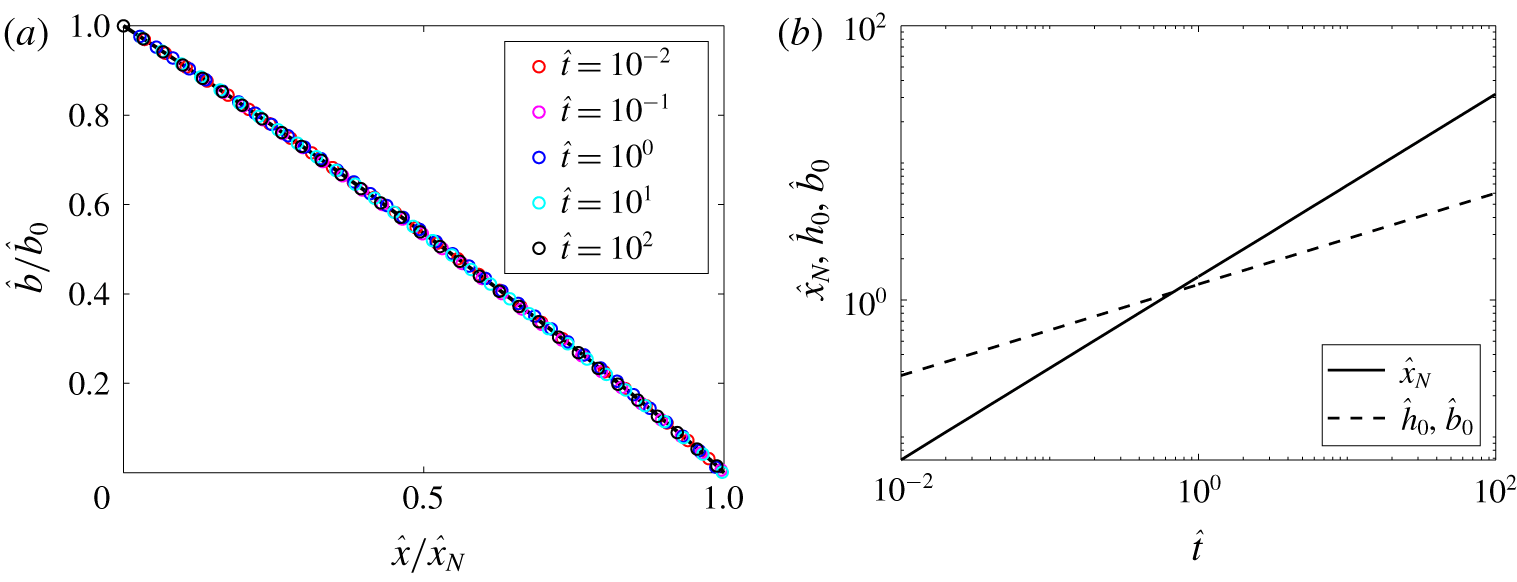
Figure 2. Numerical solutions of (2.20) and (2.21) using a finite difference scheme for: (a) dimensionless buoyancy, $\hat{b}={\hat{h}}{\hat{C}}$
, versus dimensionless length,
$\hat{b}={\hat{h}}{\hat{C}}$
, versus dimensionless length, $\hat{x}$
, at various dimensionless times,
$\hat{x}$
, at various dimensionless times, $\hat{t}$
, corresponding to (2.19), and (b)
$\hat{t}$
, corresponding to (2.19), and (b) ${\hat{h}}$
and
${\hat{h}}$
and $\hat{b}$
at
$\hat{b}$
at $\hat{x}=0$
and the nose location,
$\hat{x}=0$
and the nose location, $\hat{x}_{N}$
, as functions of
$\hat{x}_{N}$
, as functions of $\hat{t}$
.
$\hat{t}$
.
Motivated by the numerical solutions presented in § 3.1 we first look for self-similar solutions describing the evolution of the buoyancy within the current, returning to their implications for the height and concentration profiles throughout. We first note that (2.20) may be written in terms of the buoyancy, $\hat{b}={\hat{h}}{\hat{C}}$
, as
$\hat{b}={\hat{h}}{\hat{C}}$
, as
 $$\begin{eqnarray}\frac{\unicode[STIX]{x2202}\hat{b}}{\unicode[STIX]{x2202}\hat{t}}-\frac{\unicode[STIX]{x2202}}{\unicode[STIX]{x2202}\hat{x}}\left(\hat{b}\frac{\unicode[STIX]{x2202}\hat{b}}{\unicode[STIX]{x2202}\hat{x}}\right)=0,\end{eqnarray}$$
subject to
 $$\begin{eqnarray}\displaystyle -\left.\hat{b}\frac{\unicode[STIX]{x2202}\hat{b}}{\unicode[STIX]{x2202}\hat{x}}\right|_{\hat{x}=0}=1,\quad \hat{b}(\hat{x}_{N})=0,\quad \int _{0}^{\hat{x}_{N}}\hat{b}\,\text{d}\hat{x}=\hat{t}, & & \displaystyle\end{eqnarray}$$
where we have used (2.22a
) and (2.23) to write (3.3a
) and (3.3c
) respectively, and likewise used the assumption that ${\hat{h}}(\hat{x}_{N})$
is finite to rewrite (2.22d
) as (3.3b
). It is readily apparent that (3.2) and (3.3a–c
) satisfy the formulation for a sharp-interface gravity current in a porous medium (Huppert & Woods Reference Huppert and Woods1995), and hence we recover the classical result that the buoyancy is self-similar. In detail we find that
${\hat{h}}(\hat{x}_{N})$
is finite to rewrite (2.22d
) as (3.3b
). It is readily apparent that (3.2) and (3.3a–c
) satisfy the formulation for a sharp-interface gravity current in a porous medium (Huppert & Woods Reference Huppert and Woods1995), and hence we recover the classical result that the buoyancy is self-similar. In detail we find that
 $$\begin{eqnarray}\displaystyle \hat{b}=\hat{t}^{1/3}f(\unicode[STIX]{x1D702}),\quad \text{where }\unicode[STIX]{x1D702}=\frac{\hat{x}}{\hat{t}^{2/3}}\in [0,\unicode[STIX]{x1D702}_{N}] & & \displaystyle\end{eqnarray}$$
and $f(\unicode[STIX]{x1D702})$
satisfies
$f(\unicode[STIX]{x1D702})$
satisfies
 $$\begin{eqnarray}\frac{1}{3}f-\frac{2}{3}\unicode[STIX]{x1D702}\frac{\text{d}f}{\text{d}\unicode[STIX]{x1D702}}=\frac{\text{d}}{\text{d}\unicode[STIX]{x1D702}}\left(f\frac{\text{d}f}{\text{d}\unicode[STIX]{x1D702}}\right),\end{eqnarray}$$
subject to
 $$\begin{eqnarray}\displaystyle -\left.f\frac{\text{d}f}{\text{d}\unicode[STIX]{x1D702}}\right|_{0}=1,\quad f(\unicode[STIX]{x1D702}_{N})=0\quad \text{and}\quad \int _{0}^{\unicode[STIX]{x1D702}_{N}}f\,\text{d}\unicode[STIX]{x1D702}=1. & & \displaystyle\end{eqnarray}$$
Equation (3.5) is solved using a shooting method (using the Matlab routine ode45) and the result is shown in figure 3, where $f(0)=1.296$
and
$f(0)=1.296$
and $\unicode[STIX]{x1D702}_{N}=1.482$
.
$\unicode[STIX]{x1D702}_{N}=1.482$
.
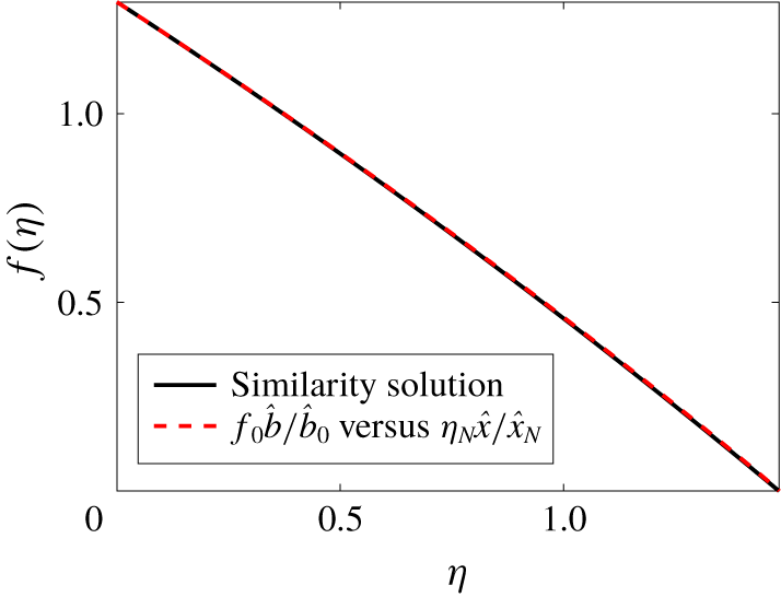
Figure 3. Numerical solution of (3.5) showing the self-similar buoyancy, or solute mass, of the gravity current. We find that $f_{0}=f(\unicode[STIX]{x1D702}=0)=1.296$
and
$f_{0}=f(\unicode[STIX]{x1D702}=0)=1.296$
and $\unicode[STIX]{x1D702}_{N}=1.482$
. The red dashed curve shows the numerical result of figure 2(a) normalized using
$\unicode[STIX]{x1D702}_{N}=1.482$
. The red dashed curve shows the numerical result of figure 2(a) normalized using $f_{0}$
and
$f_{0}$
and $\unicode[STIX]{x1D702}_{N}$
.
$\unicode[STIX]{x1D702}_{N}$
.
This result anticipates the conclusion that in the absence of entrainment, where ${\hat{C}}=1$
everywhere and hence
${\hat{C}}=1$
everywhere and hence ${\hat{h}}=\hat{b}$
, the classical, self-similar model of a gravity current in a porous medium is recovered. Furthermore this result suggests that at all times we may expect this self-similar behaviour for buoyancy, which drives the propagation of the dispersively entraining gravity current.
${\hat{h}}=\hat{b}$
, the classical, self-similar model of a gravity current in a porous medium is recovered. Furthermore this result suggests that at all times we may expect this self-similar behaviour for buoyancy, which drives the propagation of the dispersively entraining gravity current.
In contrast, dispersive entrainment dilutes the concentration within the current and adds to its apparent mass, and hence we may anticipate that the height and concentration profiles will not evolve in a self-similar manner. However, noting that ${\hat{C}}(\hat{x}=0)=1$
and hence
${\hat{C}}(\hat{x}=0)=1$
and hence ${\hat{h}}(0,\hat{t})=\hat{b}(0,\hat{t})\sim \hat{t}^{1/3}$
, we write
${\hat{h}}(0,\hat{t})=\hat{b}(0,\hat{t})\sim \hat{t}^{1/3}$
, we write
 $$\begin{eqnarray}{\hat{h}}=\hat{t}^{1/3}g(\unicode[STIX]{x1D702},\hat{t}),\end{eqnarray}$$
so that (2.21) may be rewritten as
 $$\begin{eqnarray}\frac{\unicode[STIX]{x2202}g}{\unicode[STIX]{x2202}\hat{t}}=\frac{1}{\hat{t}}\left[-\frac{g}{3}+\frac{2\unicode[STIX]{x1D702}}{3}\frac{\unicode[STIX]{x2202}g}{\unicode[STIX]{x2202}\unicode[STIX]{x1D702}}+\frac{\unicode[STIX]{x2202}g}{\unicode[STIX]{x2202}\unicode[STIX]{x1D702}}\frac{\text{d}f}{\text{d}\unicode[STIX]{x1D702}}+g\frac{\text{d}^{2}f}{\text{d}\unicode[STIX]{x1D702}^{2}}\right]-\frac{1}{\hat{t}^{2/3}}\frac{\text{d}f}{\text{d}\unicode[STIX]{x1D702}},\end{eqnarray}$$
which is subject to
 $$\begin{eqnarray}\displaystyle g(0,\hat{t})=f_{0}\quad \text{and}\quad g(\unicode[STIX]{x1D702},0)=f(\unicode[STIX]{x1D702}). & & \displaystyle\end{eqnarray}$$
Given the profile of the buoyancy, $f(\unicode[STIX]{x1D702})$
, which can be independently determined as shown previously, we see that the profile of the current, as described by
$f(\unicode[STIX]{x1D702})$
, which can be independently determined as shown previously, we see that the profile of the current, as described by $g(\unicode[STIX]{x1D702},\hat{t})$
, is governed by a purely hyperbolic (i.e. advective) equation driven by entrainment. We therefore use an upwinding discretization for
$g(\unicode[STIX]{x1D702},\hat{t})$
, is governed by a purely hyperbolic (i.e. advective) equation driven by entrainment. We therefore use an upwinding discretization for $\unicode[STIX]{x2202}g/\unicode[STIX]{x2202}\unicode[STIX]{x1D702}$
from
$\unicode[STIX]{x2202}g/\unicode[STIX]{x2202}\unicode[STIX]{x1D702}$
from $\unicode[STIX]{x1D702}=0$
, where (3.9a
) is applied, to
$\unicode[STIX]{x1D702}=0$
, where (3.9a
) is applied, to $\unicode[STIX]{x1D702}=\unicode[STIX]{x1D702}_{N}$
with the same number of grid points in between as used for
$\unicode[STIX]{x1D702}=\unicode[STIX]{x1D702}_{N}$
with the same number of grid points in between as used for $f$
in (3.5). Since
$f$
in (3.5). Since $f(\unicode[STIX]{x1D702})$
is determined independently, the values of
$f(\unicode[STIX]{x1D702})$
is determined independently, the values of $f^{\prime }$
and
$f^{\prime }$
and $f^{\prime \prime }$
at each
$f^{\prime \prime }$
at each $\unicode[STIX]{x1D702}$
used in the numerical solution for
$\unicode[STIX]{x1D702}$
used in the numerical solution for $g(\unicode[STIX]{x1D702})$
are obtained from the solution presented in figure 3. Given the
$g(\unicode[STIX]{x1D702})$
are obtained from the solution presented in figure 3. Given the $\hat{t}$
term in the denominator of (3.8), we assume that the initial condition (3.9b
) is valid at an early time
$\hat{t}$
term in the denominator of (3.8), we assume that the initial condition (3.9b
) is valid at an early time $\hat{t}=10^{-4}$
and use a time step of
$\hat{t}=10^{-4}$
and use a time step of $10^{-8}$
to solve for
$10^{-8}$
to solve for $\unicode[STIX]{x2202}g/\unicode[STIX]{x2202}\hat{t}$
explicitly, marching forward in
$\unicode[STIX]{x2202}g/\unicode[STIX]{x2202}\hat{t}$
explicitly, marching forward in $\hat{t}$
. Results for
$\hat{t}$
. Results for $g$
and
$g$
and ${\hat{C}}$
are shown in figure 4 for various values of
${\hat{C}}$
are shown in figure 4 for various values of $\hat{t}$
, where the concentration
$\hat{t}$
, where the concentration ${\hat{C}}$
is obtained from
${\hat{C}}$
is obtained from
 $$\begin{eqnarray}{\hat{C}}(\unicode[STIX]{x1D702},\hat{t})=\frac{f(\unicode[STIX]{x1D702})}{g(\unicode[STIX]{x1D702},\hat{t})}.\end{eqnarray}$$
The shock solution obtained at the nose in figure 4(a) is due to the purely advective (or hyperbolic) nature of (3.8). Furthermore, the appearance of the shock is a natural consequence of neglecting horizontal dispersion in our mathematical model. Entrainment through dispersion acts to thicken the current, ultimately leading to a large, blunt nose (see figure 4 a) and an almost linear profile of the average concentration (see figure 4 b). It is observed in figure 4(a) that at late times the height profile has a positive slope, which signifies that the volume accumulated through vertical entrainment becomes greater than the volume advected horizontally. However, the combination of the height and concentration profiles, in the form of the buoyancy (see equation (2.6)), still drives the net flow from the origin to the nose of the current, and therefore the positive slope of the height profile does not result into a backflow.

Figure 4. Numerical results obtained using an upwinding finite difference scheme for dimensionless height and concentration from (3.8) and (3.10), respectively. The dashed curve in panel (a) shows the sharp-interface solution derived by Huppert & Woods (Reference Huppert and Woods1995) which also represents $\hat{t}=0$
for the dispersive model. The solution obtained from the current, dispersive model is shown for
$\hat{t}=0$
for the dispersive model. The solution obtained from the current, dispersive model is shown for $\hat{t}=[10^{-4},10^{-3},10^{-2},10^{-1},1]$
both for
$\hat{t}=[10^{-4},10^{-3},10^{-2},10^{-1},1]$
both for $g$
and
$g$
and ${\hat{C}}$
, with arrows indicating increasing
${\hat{C}}$
, with arrows indicating increasing $\hat{t}$
.
$\hat{t}$
.
Due to the continuous entrainment from the ambient, the total volume of the current $V_{c}$
increases at a rate in excess of the injected volume,
$V_{c}$
increases at a rate in excess of the injected volume, $qt$
. The total dimensionless volume of the gravity current,
$qt$
. The total dimensionless volume of the gravity current, $\hat{V}_{c}=\unicode[STIX]{x1D719}V_{c}/(qt)$
, can therefore be written as
$\hat{V}_{c}=\unicode[STIX]{x1D719}V_{c}/(qt)$
, can therefore be written as
 $$\begin{eqnarray}\hat{V}_{c}=\frac{\unicode[STIX]{x1D719}}{qt}\int _{0}^{t}\left(\frac{q}{\unicode[STIX]{x1D719}}+\int _{0}^{x_{N}}w_{e}\,\text{d}x\right)\text{d}t=1+\frac{3}{4}\unicode[STIX]{x1D719}f_{0}\hat{t}^{1/3},\end{eqnarray}$$
where $f_{0}=1.296$
as presented in figure 3. The last term appears by combining (2.6), (2.12) and (3.4) with the similarity solution presented in figure 3. Equation (3.11) shows that the rate of entrainment is self-similar and hence the total volume of the gravity current can be predicted analytically as a function of dimensionless time
$f_{0}=1.296$
as presented in figure 3. The last term appears by combining (2.6), (2.12) and (3.4) with the similarity solution presented in figure 3. Equation (3.11) shows that the rate of entrainment is self-similar and hence the total volume of the gravity current can be predicted analytically as a function of dimensionless time $\hat{t}$
. In dimensional form, equation (3.11) reads
$\hat{t}$
. In dimensional form, equation (3.11) reads
 $$\begin{eqnarray}V_{c}=\frac{qt}{\unicode[STIX]{x1D719}}+\frac{3\unicode[STIX]{x1D6FC}f_{0}}{4\unicode[STIX]{x1D719}^{1/3}}\left[\frac{qkg\unicode[STIX]{x1D6FD}(C_{0}-C_{a})}{\unicode[STIX]{x1D708}}\right]^{2/3}t^{4/3}.\end{eqnarray}$$
This shows that when the entrainment coefficient $\unicode[STIX]{x1D6FC}=0$
,
$\unicode[STIX]{x1D6FC}=0$
, $V_{c}=qt/\unicode[STIX]{x1D719}$
, which reproduces the limiting case of the sharp-interface model. Furthermore, considering the additional volume that has entrained, a mean solute concentration
$V_{c}=qt/\unicode[STIX]{x1D719}$
, which reproduces the limiting case of the sharp-interface model. Furthermore, considering the additional volume that has entrained, a mean solute concentration $C_{c}$
, or reduced gravity, normalized by
$C_{c}$
, or reduced gravity, normalized by $C_{0}-C_{a}$
, at any
$C_{0}-C_{a}$
, at any $\hat{t}$
can be derived by buoyancy conservation as
$\hat{t}$
can be derived by buoyancy conservation as
 $$\begin{eqnarray}{\hat{C}}_{c}=\frac{C_{c}-C_{a}}{C_{0}-C_{a}}=\int _{0}^{x_{N}}\frac{\overline{C}-C_{a}}{C_{0}-C_{a}}\,\text{d}x=\frac{4}{4+3\unicode[STIX]{x1D719}f_{0}\hat{t}^{1/3}}.\end{eqnarray}$$
Thus, we find that the mean concentration of the contaminated region described by (3.13) is self-similar, which can be written in dimensional form as
 $$\begin{eqnarray}C_{c}=C_{a}+\frac{4(C_{0}-C_{a})(\unicode[STIX]{x1D719}q\unicode[STIX]{x1D708}^{2})^{1/3}}{4(\unicode[STIX]{x1D719}q\unicode[STIX]{x1D708}^{2})^{1/3}+3\unicode[STIX]{x1D719}f_{0}\unicode[STIX]{x1D6FC}[kg\unicode[STIX]{x1D6FD}(C_{0}-C_{a})]^{2/3}t^{1/3}}.\end{eqnarray}$$
4 Experimental investigation
A series of laboratory experiments were performed in which the spatial and temporal distributions of concentration were measured so as to assess the impact of dispersive mixing on the structure and dynamics of a gravity current within a porous medium. These measurements were made possible by carefully calibrating the concentration of dye, and hence colour intensity, within the experimental images. From these measurements we obtained the structure of the concentration field and were therefore able to assess the importance of dispersive mixing in the resulting gravity current.
4.1 Experimental set-up and calibration curve
The experiments were conducted in a transparent rectangular tank of size $200\times 20\times 1~\text{cm}^{3}$
. The tank was filled with
$200\times 20\times 1~\text{cm}^{3}$
. The tank was filled with $d_{p}=3.1\pm 0.2~\text{mm}$
diameter ballotini and tap water of density
$d_{p}=3.1\pm 0.2~\text{mm}$
diameter ballotini and tap water of density $\unicode[STIX]{x1D70C}_{a}=0.998~\text{g}~\text{cm}^{-3}$
. The porosity of the tank was measured and found to be
$\unicode[STIX]{x1D70C}_{a}=0.998~\text{g}~\text{cm}^{-3}$
. The porosity of the tank was measured and found to be $\unicode[STIX]{x1D719}=0.41\pm 0.01$
, which is slightly higher than the value for randomly close-packed beads (
$\unicode[STIX]{x1D719}=0.41\pm 0.01$
, which is slightly higher than the value for randomly close-packed beads ( $\unicode[STIX]{x1D719}=0.37$
) since the width of the tank is comparable with the diameter of the beads and therefore inhibits the packing. The permeability was estimated using the Kozeny–Carman relation
$\unicode[STIX]{x1D719}=0.37$
) since the width of the tank is comparable with the diameter of the beads and therefore inhibits the packing. The permeability was estimated using the Kozeny–Carman relation
 $$\begin{eqnarray}k=\frac{d_{p}^{2}}{180}\frac{\unicode[STIX]{x1D719}^{3}}{(1-\unicode[STIX]{x1D719})^{2}}\simeq 1.17\pm 0.30\times 10^{-4}~\text{cm}^{2},\end{eqnarray}$$
which compares favourably to the values $k=1.11\pm 0.17\times 10^{-4}~\text{cm}^{2}$
based on the rate of propagation of the gravity currents described below. Salt water of fixed salt and dye concentration was injected at the bottom-left corner of the tank at a constant rate during the experiments using a peristaltic pump. The water level in the tank was kept constant throughout the experiments by an overflow port at the top of the tank opposite the input port, as shown in the schematic of the experimental set-up in figure 5.
$k=1.11\pm 0.17\times 10^{-4}~\text{cm}^{2}$
based on the rate of propagation of the gravity currents described below. Salt water of fixed salt and dye concentration was injected at the bottom-left corner of the tank at a constant rate during the experiments using a peristaltic pump. The water level in the tank was kept constant throughout the experiments by an overflow port at the top of the tank opposite the input port, as shown in the schematic of the experimental set-up in figure 5.
We used a Nikon D5300 DSLR camera, with a resolution of $6000\times 4000$
pixels, to capture images of the experiments, with images recorded directly to a computer every 60 s. To ensure uniform illumination, the experimental tank was backlit by a LED light panel with the same dimensions as the tank.
$6000\times 4000$
pixels, to capture images of the experiments, with images recorded directly to a computer every 60 s. To ensure uniform illumination, the experimental tank was backlit by a LED light panel with the same dimensions as the tank.
Calibration experiments were performed to determine the functional relationship between the dye concentration and image intensity. For these experiments, the tank was uniformly saturated with a red dye of concentration $C_{d}$
. A total of 10 concentration values were used to construct the calibration curve,
$C_{d}$
. A total of 10 concentration values were used to construct the calibration curve,
 $$\begin{eqnarray}C_{d}=[0,0.02,0.05,0.10,0.20,0.40,0.60,0.80,1.00,1.20]\pm 0.01~\text{g}~\text{L}^{-1},\end{eqnarray}$$
with concentration spacing set to optimize camera sensitivity and fully resolve the calibration curve. The camera settings used were aperture $\text{f}/10$
, shutter speed
$\text{f}/10$
, shutter speed $1/2500~\text{s}$
and only the green channel of the image was used for processing. In detail, the calibration curve, shown in figure 6, was constructed by subtracting each image with non-zero dye concentration from a reference image in which
$1/2500~\text{s}$
and only the green channel of the image was used for processing. In detail, the calibration curve, shown in figure 6, was constructed by subtracting each image with non-zero dye concentration from a reference image in which $C_{d}=0$
. To account for small variations in light intensity across the tank, we divided each calibration image into a series of 1.0 (horizontal)
$C_{d}=0$
. To account for small variations in light intensity across the tank, we divided each calibration image into a series of 1.0 (horizontal) $\times$
0.3 (vertical)
$\times$
0.3 (vertical) $\text{cm}^{2}$
subregions, each containing approximately 120–150 pixels. We found that the concentration could be recovered from the image intensity in each subregion using a polynomial of the form
$\text{cm}^{2}$
subregions, each containing approximately 120–150 pixels. We found that the concentration could be recovered from the image intensity in each subregion using a polynomial of the form
 $$\begin{eqnarray}C_{d}=A(I_{0}-I)+B(I_{0}-I)^{2}~\text{g}~\text{L}^{-1},\end{eqnarray}$$
where $I$
and
$I$
and $I_{0}$
are the image intensities of the calibration image and reference image, respectively, in each subregion and
$I_{0}$
are the image intensities of the calibration image and reference image, respectively, in each subregion and $A$
and
$A$
and $B$
are their polynomial fitting coefficients. Characteristic values of
$B$
are their polynomial fitting coefficients. Characteristic values of $A$
and
$A$
and $B$
across each subregion are
$B$
across each subregion are $A=5.44\pm 1.58\times 10^{-3}~\text{g}~\text{L}^{-1}$
and
$A=5.44\pm 1.58\times 10^{-3}~\text{g}~\text{L}^{-1}$
and $B=6.73\pm 1.15\times 10^{-5}~\text{g}~\text{L}^{-1}$
.
$B=6.73\pm 1.15\times 10^{-5}~\text{g}~\text{L}^{-1}$
.
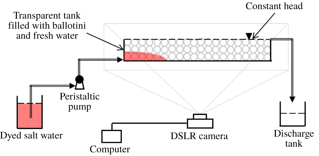
Figure 5. Schematic of the experimental set-up.
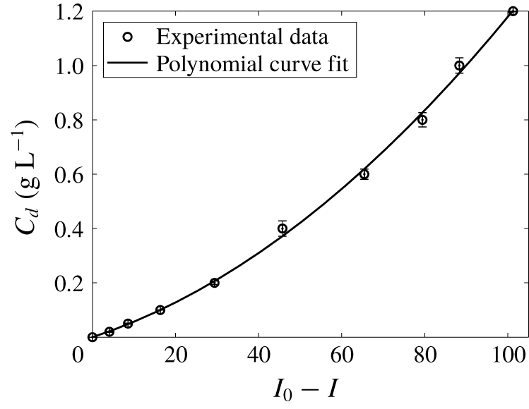
Figure 6. Calibration curve: dye concentration versus image intensity, with $C_{d}\pm 0.01~\text{g}~\text{L}^{-1}$
.
$C_{d}\pm 0.01~\text{g}~\text{L}^{-1}$
.
4.2 Gravity current experiments and concentration maps
Table 1. A summary of the experimental parameters: source volume flux $q$
, source density
$q$
, source density $\unicode[STIX]{x1D70C}_{0}$
and source reduced gravity
$\unicode[STIX]{x1D70C}_{0}$
and source reduced gravity $g_{0}^{\prime }$
, where
$g_{0}^{\prime }$
, where $g_{0}^{\prime }=g(\unicode[STIX]{x1D70C}_{0}-\unicode[STIX]{x1D70C}_{a})/\unicode[STIX]{x1D70C}_{a}\equiv g\unicode[STIX]{x1D6FD}(C_{0}-C_{a})$
. Typical measurement uncertainty of these quantities is
$g_{0}^{\prime }=g(\unicode[STIX]{x1D70C}_{0}-\unicode[STIX]{x1D70C}_{a})/\unicode[STIX]{x1D70C}_{a}\equiv g\unicode[STIX]{x1D6FD}(C_{0}-C_{a})$
. Typical measurement uncertainty of these quantities is $q\pm 0.001~\text{cm}^{2}~\text{s}^{-1}$
,
$q\pm 0.001~\text{cm}^{2}~\text{s}^{-1}$
, $\unicode[STIX]{x1D70C}_{0}\pm 0.005~\text{g}~\text{cm}^{-3}$
and
$\unicode[STIX]{x1D70C}_{0}\pm 0.005~\text{g}~\text{cm}^{-3}$
and $g_{0}^{\prime }\pm 0.52~\text{cm}~\text{s}^{-2}$
, respectively. Also presented in the table are the standard deviations of the errors
$g_{0}^{\prime }\pm 0.52~\text{cm}~\text{s}^{-2}$
, respectively. Also presented in the table are the standard deviations of the errors $\text{err}$
, calculated using (4.4), involved with the post-processing scheme in measuring the concentration and volume within the currents from the start to end of each experiment.
$\text{err}$
, calculated using (4.4), involved with the post-processing scheme in measuring the concentration and volume within the currents from the start to end of each experiment.

A suite of gravity current experiments was conducted in which the fixed source volume flux $q$
and fluid density
$q$
and fluid density $\unicode[STIX]{x1D70C}_{0}$
, or equivalently concentration
$\unicode[STIX]{x1D70C}_{0}$
, or equivalently concentration $C_{0}$
, were varied. In total, we report on 10 experiments, for which the details are listed in table 1, where experiments 4 and 7 are repeats of experiments 3 and 6 respectively. The images from these experiments were processed in a manner consistent with the calibration experiments: they were first cropped and subtracted from a reference image taken of the tank saturated with tap water just before starting each experiment. The image intensity of these processed images was then converted into a concentration,
$C_{0}$
, were varied. In total, we report on 10 experiments, for which the details are listed in table 1, where experiments 4 and 7 are repeats of experiments 3 and 6 respectively. The images from these experiments were processed in a manner consistent with the calibration experiments: they were first cropped and subtracted from a reference image taken of the tank saturated with tap water just before starting each experiment. The image intensity of these processed images was then converted into a concentration, $C_{d}(x,z,t)$
using the calibration curve (4.3) in each
$C_{d}(x,z,t)$
using the calibration curve (4.3) in each $0.3~\text{cm}^{2}$
subregion. An example of the processed experimental images is shown in figure 7 where the raw gravity current images and the processed concentration maps are shown from a representative experiment (experiment 7) at four time points.
$0.3~\text{cm}^{2}$
subregion. An example of the processed experimental images is shown in figure 7 where the raw gravity current images and the processed concentration maps are shown from a representative experiment (experiment 7) at four time points.
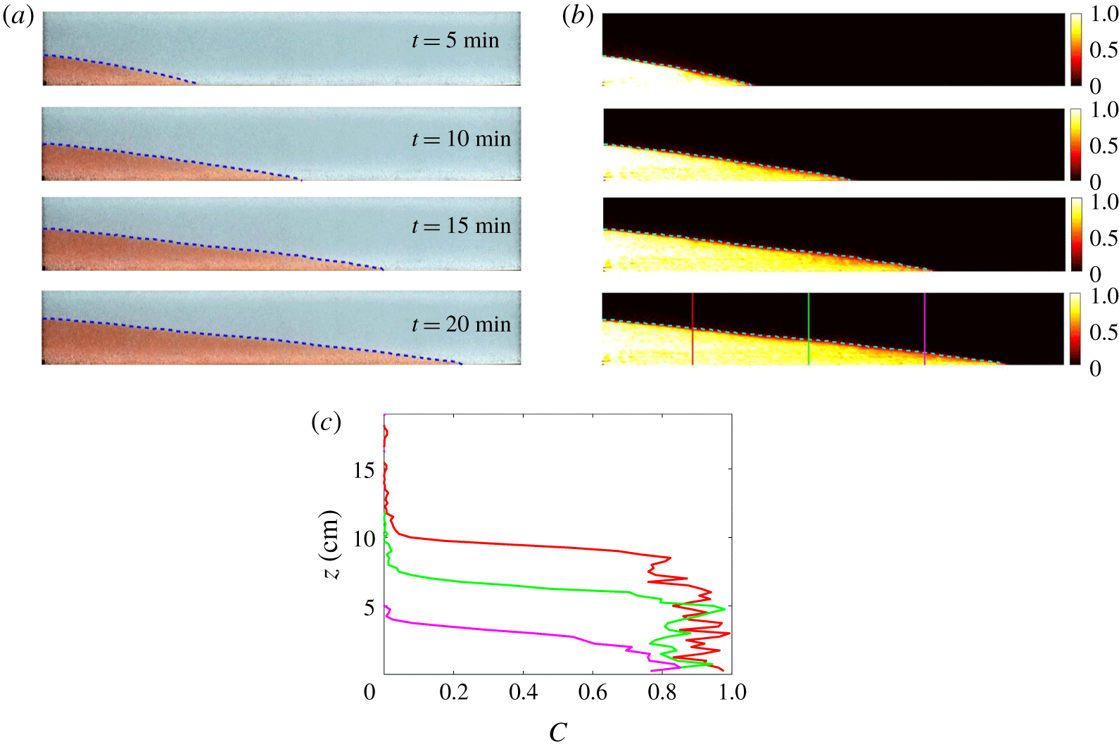
Figure 7. (a) Gravity current images, (b) their concentration maps and (c) vertical concentration profiles. Dashed curves represent the height profiles obtained using interface detection algorithm. Each individual panel is 200 cm long and 20 cm tall, whereas the colour map scale represents $(C-C_{a})/(C_{0}-C_{a})$
. In (c) the red, green and magenta curves represent the vertical concentration variation at three different locations indicated in the concentration map at
$(C-C_{a})/(C_{0}-C_{a})$
. In (c) the red, green and magenta curves represent the vertical concentration variation at three different locations indicated in the concentration map at $t=20~\text{min}$
.
$t=20~\text{min}$
.
To measure the height profiles of the gravity currents we use an interface detection method on the image intensity or concentration which does not rely on the calibration data. After subtracting the gravity current images from a reference image the resultant image is divided into vertical columns of 1 cm thickness across the tank. For each column the vertical gradient of the intensity, indirectly the concentration gradient, is calculated. From these intensity or concentration gradients, the location of the maximum absolute gradient is taken as the interface between the gravity current and ambient fluid. Height profiles obtained through this interface detection method are shown using dashed curves in figure 7, both in the raw images and on the concentration maps.
Furthermore, we note that the concentration maps in figure 7 are uniform to leading order, but contain a concentration profile that varies systematically across the current. We divided the concentration maps into vertical columns of equal thickness and the mean vertical concentration for each column was calculated. Also presented in figure 7 are the vertical variations of concentration at three different locations, shown in red, green and magenta. The clear difference in concentration between these three curves at $z\rightarrow 0$
, signifies the horizontal variation, whereas their individual vertical variations correspond to the assumption we made in § 2.1, i.e. shown figure 1, that maximum concentration gradient occurs at the edge and remains nearly constant beneath that.
$z\rightarrow 0$
, signifies the horizontal variation, whereas their individual vertical variations correspond to the assumption we made in § 2.1, i.e. shown figure 1, that maximum concentration gradient occurs at the edge and remains nearly constant beneath that.
As a check on the accuracy of the dye-concentration calibration scheme, we calculate the normalized difference between the concentration injected, and that imaged in the entire tank at any time $t$
. The percentage error, defined in this way, is therefore given by
$t$
. The percentage error, defined in this way, is therefore given by
 $$\begin{eqnarray}\text{err}=\left[\frac{qt(C_{0}-C_{a})}{\unicode[STIX]{x1D719}}-V_{c}C_{c}\right]\frac{100\unicode[STIX]{x1D719}}{qt(C_{0}-C_{a})},\end{eqnarray}$$
where $V_{c}$
and
$V_{c}$
and $C_{c}$
are the total volume and mean concentration of the contaminated region measured using the dye-attenuation image processing routine at time
$C_{c}$
are the total volume and mean concentration of the contaminated region measured using the dye-attenuation image processing routine at time $t$
for an experiment of volume flux
$t$
for an experiment of volume flux $q$
and source concentration
$q$
and source concentration $C_{0}$
. The percentage error,
$C_{0}$
. The percentage error, $\text{err}$
, is estimated for each experiment at 10 different times from the start to end of the experiment. The values are found to be random and do not show any particular trend in time. Standard deviations of these errors are presented in table 1 and are encouragingly within
$\text{err}$
, is estimated for each experiment at 10 different times from the start to end of the experiment. The values are found to be random and do not show any particular trend in time. Standard deviations of these errors are presented in table 1 and are encouragingly within $\pm 2.5\,\%$
for each case.
$\pm 2.5\,\%$
for each case.
4.3 Comparison with dispersive entrainment theory

Figure 8. Log–log plot of total entrained volume in gravity currents versus time. The straight lines represent theoretical predictions from (3.12) with the best fit $\unicode[STIX]{x1D6FC}=0.013\pm 0.005$
.
$\unicode[STIX]{x1D6FC}=0.013\pm 0.005$
.
The raw gravity current images and concentration maps in figure 7 verify the occurrence of entrainment in gravity currents in porous media. To quantitively analyse the effects of entrainment and compare the results of our experiments with our theoretical predictions we first estimate the value of the entrainment coefficient $\unicode[STIX]{x1D6FC}$
. We consider the total entrained volume (
$\unicode[STIX]{x1D6FC}$
. We consider the total entrained volume ( $V_{c}-qt/\unicode[STIX]{x1D719}$
) as the basis for a global estimate of
$V_{c}-qt/\unicode[STIX]{x1D719}$
) as the basis for a global estimate of $\unicode[STIX]{x1D6FC}$
, whose theoretical predictions are obtained from (3.12) and experimental values from the concentration maps in figure 7. A best fit analysis of the quantity
$\unicode[STIX]{x1D6FC}$
, whose theoretical predictions are obtained from (3.12) and experimental values from the concentration maps in figure 7. A best fit analysis of the quantity $V_{c}-qt/\unicode[STIX]{x1D719}$
is performed and compared to the theoretical predictions for each experiment, which suggests
$V_{c}-qt/\unicode[STIX]{x1D719}$
is performed and compared to the theoretical predictions for each experiment, which suggests $\unicode[STIX]{x1D6FC}=0.013\pm 0.005$
and is shown in figure 8. The vertical and horizontal axes represent the left and right (without
$\unicode[STIX]{x1D6FC}=0.013\pm 0.005$
and is shown in figure 8. The vertical and horizontal axes represent the left and right (without $\unicode[STIX]{x1D6FC}$
) terms in (3.12), respectively, and the straight lines are the theoretical predictions. The data are consistent with the simple, linear entrainment law used, particularly at later times, with discrepancies between theory and experiment at early times likely amplified by the relaxation of the source flow to a long, thin gravity current.
$\unicode[STIX]{x1D6FC}$
) terms in (3.12), respectively, and the straight lines are the theoretical predictions. The data are consistent with the simple, linear entrainment law used, particularly at later times, with discrepancies between theory and experiment at early times likely amplified by the relaxation of the source flow to a long, thin gravity current.
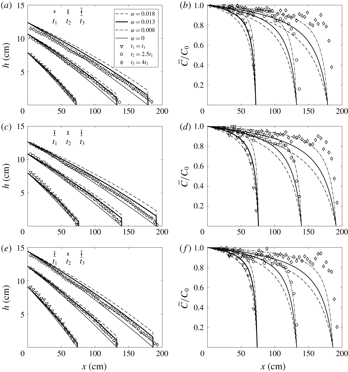
Figure 9. Comparison of theory versus experiment for $h$
and
$h$
and $\overline{C}$
: (a,b) experiment 1, (c,d) experiment 6 and (e,f) experiment 8. Results are presented for three different times with
$\overline{C}$
: (a,b) experiment 1, (c,d) experiment 6 and (e,f) experiment 8. Results are presented for three different times with $t_{1}=[12,6,5]~\text{min}$
for experiments 1, 6 and 8, respectively. Indicative error bars for the height profiles are shown at the top left corners in each panel for times
$t_{1}=[12,6,5]~\text{min}$
for experiments 1, 6 and 8, respectively. Indicative error bars for the height profiles are shown at the top left corners in each panel for times $t_{1}$
,
$t_{1}$
, $t_{2}$
and
$t_{2}$
and $t_{3}$
. These error bars represent the mean difference between the height measured and the height predicted using
$t_{3}$
. These error bars represent the mean difference between the height measured and the height predicted using $\unicode[STIX]{x1D6FC}=0.013$
for each time.
$\unicode[STIX]{x1D6FC}=0.013$
for each time.
The height profiles of the experimental gravity currents are presented in figure 9 for three different experiments at three different times, where the time span is different for each experiment. The experimental results are compared with the predictions of our dispersive model for $\unicode[STIX]{x1D6FC}=0.008$
, 0.013 and 0.018, consistent with figure 8, and the height profiles predicted by the sharp-interface model, i.e.
$\unicode[STIX]{x1D6FC}=0.008$
, 0.013 and 0.018, consistent with figure 8, and the height profiles predicted by the sharp-interface model, i.e. $\unicode[STIX]{x1D6FC}=0$
(Huppert & Woods Reference Huppert and Woods1995). At early times (
$\unicode[STIX]{x1D6FC}=0$
(Huppert & Woods Reference Huppert and Woods1995). At early times ( $t_{1}$
in each panel) the dispersive and sharp-interface predictions almost coincide, whereas at later times the difference between them increases gradually as the accumulated mixing increases. This behaviour is confirmed by our experiments, as the discrete experimental data show a good agreement with the dispersive height profiles and tend to evolve a blunted nose at the front due to entrainment. Encouragingly, most of the experimental data fall between the height profiles predicted for
$t_{1}$
in each panel) the dispersive and sharp-interface predictions almost coincide, whereas at later times the difference between them increases gradually as the accumulated mixing increases. This behaviour is confirmed by our experiments, as the discrete experimental data show a good agreement with the dispersive height profiles and tend to evolve a blunted nose at the front due to entrainment. Encouragingly, most of the experimental data fall between the height profiles predicted for $\unicode[STIX]{x1D6FC}=0.013\pm 0.005$
.
$\unicode[STIX]{x1D6FC}=0.013\pm 0.005$
.
In the concentration plots of figure 9 (right side panels) we find that the spatio-temporal variation of mean concentration is in agreement with the theoretical predictions, which we have plotted for three different values of $\unicode[STIX]{x1D6FC}$
similar to that for the height profiles – note that, according to our theoretical model, the length of the gravity current,
$\unicode[STIX]{x1D6FC}$
similar to that for the height profiles – note that, according to our theoretical model, the length of the gravity current, $x_{N}$
, is unaffected by the entrainment and therefore the predictions for different
$x_{N}$
, is unaffected by the entrainment and therefore the predictions for different $\unicode[STIX]{x1D6FC}$
in figure 9 converge at the nose. The experimental data highlight the effect of mixing, with a decreasing concentration towards the front of the current, as predicted by the dispersive entrainment model. In comparison, the mean concentration predicted by the sharp-interface model is
$\unicode[STIX]{x1D6FC}$
in figure 9 converge at the nose. The experimental data highlight the effect of mixing, with a decreasing concentration towards the front of the current, as predicted by the dispersive entrainment model. In comparison, the mean concentration predicted by the sharp-interface model is $C(x,t)=1$
. While these concentration plots show a clear demonstration of mixing in experiments, we observe that at late times the data around the nose are quite dispersed and they deviate significantly from the predictions. This may be either because the gravity current closer to the nose is much thinner, which makes it more prone to the errors linked with the post-processing scheme we use for making the concentration maps or because the horizontal entrainment is significant at the nose which we do not consider in our theoretical model.
$C(x,t)=1$
. While these concentration plots show a clear demonstration of mixing in experiments, we observe that at late times the data around the nose are quite dispersed and they deviate significantly from the predictions. This may be either because the gravity current closer to the nose is much thinner, which makes it more prone to the errors linked with the post-processing scheme we use for making the concentration maps or because the horizontal entrainment is significant at the nose which we do not consider in our theoretical model.

Figure 10. Comparison of theory versus experiment for the buoyancy flux. Black curve represent the prediction shown in figure 3 and the discrete data are from experiments 1, 6 and 8 at three different times.
In figure 10 we show the buoyancy $(b=h\overline{C})$
profiles for the experiments presented in figure 9 by combining the left and right panels at the respective times. All the data are normalized using the buoyancy at
$(b=h\overline{C})$
profiles for the experiments presented in figure 9 by combining the left and right panels at the respective times. All the data are normalized using the buoyancy at $x=0$
,
$x=0$
, $b_{0}$
, and length
$b_{0}$
, and length $x_{N}$
such that they collapse onto a universal profile, thus demonstrating the self-similarity of the buoyancy flux. The self-similar profile (solid curve) obtained from figure 3 shows a good agreement with the discrete experimental data.
$x_{N}$
such that they collapse onto a universal profile, thus demonstrating the self-similarity of the buoyancy flux. The self-similar profile (solid curve) obtained from figure 3 shows a good agreement with the discrete experimental data.

Finally, we compare the length ( $x_{N}$
) and height at the source (
$x_{N}$
) and height at the source ( $h_{0}$
) of the gravity currents for all 10 experiments from table 1 as shown in figure 11. Here,
$h_{0}$
) of the gravity currents for all 10 experiments from table 1 as shown in figure 11. Here, $\hat{x}_{N}$
,
$\hat{x}_{N}$
, ${\hat{h}}_{0}$
and
${\hat{h}}_{0}$
and $\hat{t}$
are the non-dimensional quantities defined in (2.19) and the straight lines represent the predictions from (3.4) and (3.7), respectively, with
$\hat{t}$
are the non-dimensional quantities defined in (2.19) and the straight lines represent the predictions from (3.4) and (3.7), respectively, with $\unicode[STIX]{x1D702}=\unicode[STIX]{x1D702}_{N}=1.482$
and
$\unicode[STIX]{x1D702}=\unicode[STIX]{x1D702}_{N}=1.482$
and $g=f_{0}=1.296$
. Agreement between the theory and experiments is promising, with minor deviation in panel (b) for
$g=f_{0}=1.296$
. Agreement between the theory and experiments is promising, with minor deviation in panel (b) for $h_{0}$
. This deviation may be attributed to the fact that the ambient fluid motion is neglected in our theoretical analysis, whereas in the experiments
$h_{0}$
. This deviation may be attributed to the fact that the ambient fluid motion is neglected in our theoretical analysis, whereas in the experiments $h_{0}$
is of the order of ambient fluid depth.
$h_{0}$
is of the order of ambient fluid depth.
5 Discussion
The mixing of fluids in porous media is a long-standing problem with a large number of important geophysical and industrial applications. To date, many approaches to modelling mixing, or dispersion, within porous media have focused on augmented advection–diffusion models. Here, motivated by highly successful models of turbulent plumes and gravity currents, we have instead sought to constrain only the bulk properties of the gravity current, the mass and the concentration or buoyancy. While such conservation arguments neglect the variance inherent in the flows, they are a powerful tool for understanding the large-scale dynamics.
Through a set of careful laboratory experiments we have tested the predicted consequences of such a dispersive entrainment model, and find good agreement when analysing the structure of the depth-averaged concentration in particular (see figure 9).
We see a clear indication of entrainment in the laboratory experiments through the increasing volume with time (see figure 8). However, we see only a minor difference between our dispersive model and the sharp-interface model predictions, particularly for height profiles (figure 9), although we note that the laboratory experiments generally fall in a range where dimensionless time $\hat{t}<10^{-3}$
. At these early times the total entrainment is small, increasing the volume of the current by only approximately 4 % (see (3.11)). When the gravity currents are allowed to develop for longer, e.g. in real geological flows where
$\hat{t}<10^{-3}$
. At these early times the total entrainment is small, increasing the volume of the current by only approximately 4 % (see (3.11)). When the gravity currents are allowed to develop for longer, e.g. in real geological flows where $\hat{t}$
can become much larger, the discrepancy between the sharp-interface model and actual flow may increase with time and in these cases dispersive mixing would become more significant. We also anticipate that as time progresses and dispersive entrainment leads to the formation of a shock front at the nose, longitudinal dispersion may become more significant, an effect we here neglected in this study.
$\hat{t}$
can become much larger, the discrepancy between the sharp-interface model and actual flow may increase with time and in these cases dispersive mixing would become more significant. We also anticipate that as time progresses and dispersive entrainment leads to the formation of a shock front at the nose, longitudinal dispersion may become more significant, an effect we here neglected in this study.
The importance or magnitude of the dispersive entrainment depends crucially on the small-scale structure of the porous medium. Here, for mathematical and experimental simplicity, we have focused on pore-scale dispersion for which the effective entrainment coefficient is necessarily small. However, for many natural systems the effective dispersion may be much larger, particularly when considering heterogeneities at the 10 cm scale acting on currents which are 1–10 m thick. In such cases the effective entrainment would necessarily reflect the underlying structure of the medium, appropriately averaged.
In many heterogeneous media the dispersivity becomes dependent on the scale of the flow because of resultant flow instabilities and local non-uniform velocities (Wheatcarft & Tyler Reference Wheatcarft and Tyler1988; Gelhar Reference Gelhar1992). An example of enhanced entrainment can be seen in the two-layered experiments of Huppert et al. (Reference Huppert, Neufeld and Strandkvist2013, figure 7) and Sahu & Flynn (Reference Sahu and Flynn2017, figure 4). In these cases the entrainment is enhanced because of a layered permeability structure which results in Rayleigh–Taylor instabilities which actively promote mixing.
The experimental images of Huppert et al. (Reference Huppert, Neufeld and Strandkvist2013) and Sahu & Flynn (Reference Sahu and Flynn2017) also show that the gravity current is significantly thicker at the nose even at the laboratory scale than seen in the homogenous cases (see figure 9). This is consistent with our findings shown in figure 4(a) for larger $\hat{t}$
, which is greater in those experiments due to enhanced
$\hat{t}$
, which is greater in those experiments due to enhanced $\unicode[STIX]{x1D6FC}$
.
$\unicode[STIX]{x1D6FC}$
.
While the total volume of entrained fluid increases with time due to the increasing interfacial area, the entrainment rate, $w_{e}$
(see (2.12)) decreases because the horizontal velocity of the current decreases as
$w_{e}$
(see (2.12)) decreases because the horizontal velocity of the current decreases as $u\propto t^{-1/3}$
as can be inferred from (2.6) and (3.4). This implies that the Péclet number
$u\propto t^{-1/3}$
as can be inferred from (2.6) and (3.4). This implies that the Péclet number $Pe\propto t^{-1/3}$
(see (2.13)), and therefore at late times the effects of dispersion may no longer be dominant.
$Pe\propto t^{-1/3}$
(see (2.13)), and therefore at late times the effects of dispersion may no longer be dominant.
The time scale for the transition between dispersive (advective) and diffusive behaviour can be estimated by considering the velocity at the nose,
 $$\begin{eqnarray}u_{N}=\unicode[STIX]{x1D719}\frac{\text{d}x_{N}}{\text{d}t}=\frac{2}{3}\unicode[STIX]{x1D702}_{N}\left(\frac{\unicode[STIX]{x1D719}kg\unicode[STIX]{x1D6FD}C_{0}q}{\unicode[STIX]{x1D708}}\right)^{1/3}\frac{1}{t^{1/3}},\end{eqnarray}$$
which is characteristic of velocities within the current. The time at which the current reaches $Pe\lesssim 1$
can then be straightforwardly given as
$Pe\lesssim 1$
can then be straightforwardly given as
 $$\begin{eqnarray}t_{D}=\frac{\unicode[STIX]{x1D719}kg\unicode[STIX]{x1D6FD}C_{0}q}{\unicode[STIX]{x1D708}}\left(\frac{2}{3}\frac{\unicode[STIX]{x1D70F}d_{p}\unicode[STIX]{x1D702}_{N}}{D_{m}}\right)^{3}.\end{eqnarray}$$
At times $t>t_{D}$
diffusion may become significant, and thus the nature of entrainment may change. In addition, over time
$t>t_{D}$
diffusion may become significant, and thus the nature of entrainment may change. In addition, over time $t\sim O(t_{D})$
the front of the gravity current may develop a shock-type structure implying that the assumption of negligible lateral entrainment is no longer valid.
$t\sim O(t_{D})$
the front of the gravity current may develop a shock-type structure implying that the assumption of negligible lateral entrainment is no longer valid.
A related analysis of the mixing of miscible fluids in a confined gravity current in a porous medium was conducted by Szulczewski & Juanes (Reference Szulczewski and Juanes2013). In their analysis Szulczewski & Juanes (Reference Szulczewski and Juanes2013) consider only molecular diffusion, and show that there are five dominant regimes of mixing: an early-time diffusive regime, an S-slumping regime, a straight-line slumping regime, a Taylor-slumping regime and a late-time diffusive regime. In the first and last regimes they show that the mixing between the gravity current and ambient occurs purely due to molecular diffusion and the concentration follows an error-function distribution, where solute mass flux, $F$
, across a vertical cross-section varies in time as
$F$
, across a vertical cross-section varies in time as $F\propto t^{-1/2}$
. In the S-slumping regime the mass flux is independent of time, whereas in the straight-line and Taylor-slumping regimes, the flux
$F\propto t^{-1/2}$
. In the S-slumping regime the mass flux is independent of time, whereas in the straight-line and Taylor-slumping regimes, the flux $F\propto t^{-1/2}$
and
$F\propto t^{-1/2}$
and $F\propto t^{-3/4}$
, respectively. In our analysis the flux
$F\propto t^{-3/4}$
, respectively. In our analysis the flux $F\sim uC$
and, in contrast to the work of Szulczewski & Juanes (Reference Szulczewski and Juanes2013), follows a single dependence on time as
$F\sim uC$
and, in contrast to the work of Szulczewski & Juanes (Reference Szulczewski and Juanes2013), follows a single dependence on time as $F\propto t^{-1/3}$
up to times
$F\propto t^{-1/3}$
up to times $t\sim t_{D}$
. However, it is important to note that our results differ from those of Szulczewski & Juanes (Reference Szulczewski and Juanes2013) both in that we consider a velocity-dependent dispersion (rather than a molecular diffusivity), and because we consider the case of continuous flux injection in an unconfined ambient in contrast to the fixed volumes of dense and ambient fluid and a confined boundary. Flows in confined settings are likely to generate significant vertical sheer, such that the feedback between the flow and the concentration distribution may not satisfy the simple approximations model here which are more appropriate for unconfined flows.
$t\sim t_{D}$
. However, it is important to note that our results differ from those of Szulczewski & Juanes (Reference Szulczewski and Juanes2013) both in that we consider a velocity-dependent dispersion (rather than a molecular diffusivity), and because we consider the case of continuous flux injection in an unconfined ambient in contrast to the fixed volumes of dense and ambient fluid and a confined boundary. Flows in confined settings are likely to generate significant vertical sheer, such that the feedback between the flow and the concentration distribution may not satisfy the simple approximations model here which are more appropriate for unconfined flows.
6 Conclusion
Motivated by the importance of mixing in geological flows, we have described a modelling approach for understanding dispersive entrainment in gravity currents in porous media. The mathematical model conserves mass and concentration, or buoyancy, within the current and considers the addition of mass to the current through a dispersive interface. For simplicity we assume that the entrainment is proportional to the velocity of the current and may be characterized by a constant entrainment coefficient.
Here, we show that a natural consequence of the model is that the buoyancy flux of the current exhibits a self-similar behaviour and does not depend on the details of the dispersive entrainment. Using a modified similarity solution we then derive the height profiles and concentration of the gravity current, which prove to not be self-similar in nature, and show that the shape of the current and the concentration change with time. However, the total amount of entrainment and the mean concentration of the contaminated region are self-similar and vary with dimensionless time as $\hat{t}^{1/3}$
and
$\hat{t}^{1/3}$
and $\hat{t}^{-1/3}$
, respectively. We note that the resulting model recovers classical models of gravity currents in porous media when dispersive entrainment is negligible.
$\hat{t}^{-1/3}$
, respectively. We note that the resulting model recovers classical models of gravity currents in porous media when dispersive entrainment is negligible.
We also present laboratory experiments which were performed using a dye-attenuation technique. We first performed calibration experiments to find a functional relationship between the dye concentration and image intensity. These calibration data were then used to determine the concentration in the gravity current experiments. A total of 10 experiments were performed with varying volume flux and concentration at the source as variables. For these experiments we find that the volume of the current grows measurably by entrainment, and that the entrainment coefficient $\unicode[STIX]{x1D6FC}=0.013\pm 0.005$
. Furthermore, the experimental results independently confirm the occurrence of entrainment in porous medium gravity currents and in general show a good agreement with the predictions of our dispersive interface model.
$\unicode[STIX]{x1D6FC}=0.013\pm 0.005$
. Furthermore, the experimental results independently confirm the occurrence of entrainment in porous medium gravity currents and in general show a good agreement with the predictions of our dispersive interface model.
We predict that at late times, when the velocity of the gravity current becomes significantly small, it may be sensible to consider the effects of molecular diffusion and also discard the assumption of long and thin current.
The modelling framework presented here, along with the experimental methodology, provide a new approach to characterizing mixing in porous media. In particular, we anticipate that the approach may provide a significant simplification in cases where the porous medium is heterogeneous across a range of scales. In addition, the transition between dispersive entrainment, dominated by rapid advection, to late-time diffusive mixing may yet be incorporated in such an averaged model with implications for the ultimate fate of sequestered $\text{CO}_{2}$
, for example.
$\text{CO}_{2}$
, for example.
Acknowledgements
This research is a contribution from the GeoCquest consortium, a BHP-supported collaborative project between the Cambridge, Stanford, and Melbourne Universities. J.A.N. is partly supported through a Royal Society University Research Fellowship.


 Open access