


1. Introduction
Vortex dominated flow physics behind oscillating plates and airfoils in low Reynolds number ( $Re$) regime has been studied quite extensively in the literature. These studies have been inspired from the optimum lift and thrust generation capabilities observed in different biological phyla, such as insects, birds and fishes, through an excellent interplay between flapping wings/fins and the flow field vortices. Recent research interests in this field also stem from the need for designing biomimetic robotic devices, such as flapping wing microaerial vehicles (known as MAVs) and autonomous underwater vehicles (known as AUVs) (Triantafyllou, Triantafyllou & Yue Reference Triantafyllou, Triantafyllou and Yue2000; Platzer et al. Reference Platzer, Jones, Young and Lai2008; Shyy et al. Reference Shyy, Aono, Chimakurthi, Trizila, Kang, Cesnik and Liu2010). The aerodynamic performance of flapping airfoils in pure pitching (Koochesfahani Reference Koochesfahani1989; Godoy-Diana, Aider & Wesfreid Reference Godoy-Diana, Aider and Wesfreid2008; Schnipper Reference Schnipper2010) and pure heaving (Jones, Dohring & Platzer Reference Jones, Dohring and Platzer1998; Lai & Platzer Reference Lai and Platzer1999; Lewin & Haj-Hariri Reference Lewin and Haj-Hariri2003; Heathcote & Gursul Reference Heathcote and Gursul2007) has been studied quite extensively. However, the literature on combined pitching–heaving kinematics is relatively limited (Anderson et al. Reference Anderson, Streitlien, Barrett and Triantafyllou1998; Read, Hover & Triantafyllou Reference Read, Hover and Triantafyllou2003; Von Ellenrieder, Parker & Soria Reference Von Ellenrieder, Parker and Soria2003; Van Buren, Floryan & Smits Reference Van Buren, Floryan and Smits2019). The present study considers a canonical pitch–heave flapping model for investigating the transitional behaviour of the far-field wake as the flow dynamics approaches chaos. The unsteady load generation mechanisms of flapping foils are inherently linked with the nature of the wake interactions around them, and chaotic flow field would result in unfavourable load conditions from the control point of view of man-made flapping devices. It is of considerable importance to have an appropriate understanding of the transitional flow-dynamics around flapping foils for the efficient design and development of control algorithms for nature-inspired flapping devices to ensure their stable operations. Furthermore, the novelty of the present study lies in filling in the gaps in the existing literature on the transitional wake patterns of a flapping airfoil beyond the periodic regime, which is rarely addressed in the literature from a combined viewpoint of the behaviour of flow field vortices and nonlinear dynamics.
The existing literature categorises the flow field in a variety of trailing-wake patterns depending on the amplitude-based Strouhal number,  $St_A =2fA/U_\infty$ (Anderson et al. Reference Anderson, Streitlien, Barrett and Triantafyllou1998), where $A$ and $f$ are the flapping amplitude and frequency, respectively, and $U_\infty$ is the free stream velocity. The dynamic heave velocity ( $\kappa h$), which is proportional to $St_A$, has also been commonly used in this regard; $h$ (
$h$ ( ${=}A/c$) is the non-dimensional stroke amplitude, $\kappa$ ( ${=}2 {\rm \pi}f c/U_\infty$) is the reduced frequency and $c$ is chord length of the airfoil. As $\kappa h$ is increased to a high value ( $\kappa h > 1.50$), the periodicity of the wake is gradually lost and the wake transitions to aperiodicity. This has been investigated for heaving airfoils in a series of studies – see Lewin & Haj-Hariri (Reference Lewin and Haj-Hariri2003), Ashraf, Young & Lai (Reference Ashraf, Young and Lai2012), Martín-Alcántara, Fernandez-Feria & Sanmiguel-Rojas (Reference Martín-Alcántara, Fernandez-Feria and Sanmiguel-Rojas2015) and Khalid et al. (Reference Khalid, Akhtar, Dong, Ahsan, Jiang and Wu2018). Most of them have reported a quasi-periodic transition to chaos, though no rigorous dynamical tests were used to establish this route. Badrinath, Bose & Sarkar (Reference Badrinath, Bose and Sarkar2017) have observed the presence of an intermittency route to chaos in pure heaving and have also established the dynamics using classical and non-classical tools based on nonlinear dynamical theories. For a pitching airfoil as well, a quasi-periodic route to chaos was reported at high pitch amplitudes by Zaman, Young & Lai (Reference Zaman, Young and Lai2017). Recently, Deng et al. (Reference Deng, Sun, Teng, Pan and Shao2016) have observed chaotic flow patterns for both pure heaving and pure pitching separately, though the authors did not comment on the nature of the transition route.
To the best of the authors’ knowledge, similar studies for a combined pitching–heaving airfoil are hard to find, notable exceptions being the studies reported by Lentink and his coworkers (Lentink et al. Reference Lentink, Muijres, Donker-Duyvis and van Leeuwen2008, Reference Lentink, Van Heijst, Muijres and Van Leeuwen2010). Also, very recently, Bose & Sarkar (Reference Bose and Sarkar2018) considered a pitching–heaving case and observed a quasi-periodic transition to chaos in the near-field patterns. Each dynamical state and the transitions were established using robust measures from dynamical systems theories. The authors further investigated the role of leading-edge vortices (LEVs) in triggering aperiodicity in the near-field. Nonlinear time series analyses were undertaken using the time histories of the aerodynamic loads, which directly reflect the near-field behaviour. A study of the far-field dynamics in the same parametric regime was not attempted by the authors. While the near-field holds the key to understanding the trigger to aperiodicity, far-field patterns reveal the development of the wake and its long term evolution. As the near-field and far-field dynamics are related, one would also expect the far-field to lose its periodicity; however, the underlying mechanism needs to be established. Although some interesting observations of the far-field wake patterns, such as loss of stability of a deflected reverse Kármán wake and irregular jet-switching, have been reported in the literature, chaos has not been reported in the far-field wake. Furthermore, these interesting far-field patterns have not been linked to the near-field transition behaviour. The present study investigates the transition route to chaos in the far-field wake, the influence of the near-field on its transitions and the spatio-temporal behaviour that leads to aperiodicity and chaos, while a dynamic interlinking of the far-wake with the near-field interactions is sought.
Though the far-field wake in the periodic but deflected regime has been studied widely, a few questions have remained unanswered. For example, the role of LEVs has not been addressed. Godoy-Diana et al. (Reference Godoy-Diana, Marais, Aider and Wesfreid2009) have studied the mechanism of wake deflection by modelling the self-advection and relative phase velocities of two consecutive vortex dipoles. Zheng & Wei (Reference Zheng and Wei2012) supported these findings and also proposed an extension to this wake model. Recently, He & Gursul (Reference He and Gursul2016) have also proposed a simplified point-vortex-based model to investigate the criterion of symmetry breaking deflection in the wake. Though these simplified artefacts can provide some answers to the mechanism of wake deflection, they cannot capture the effect of the LEVs in it. The role of the LEVs on the transition of the wake from deflected periodic to aperiodic and chaotic patterns is also unknown. On the other hand, LEVs have been reported to provide the first trigger for the aperiodic transition in the near-field, as reported by Bose & Sarkar (Reference Bose and Sarkar2018). The mechanism of propagation of aperiodicity from near- to far-field and the significance of the LEVs need further investigation. It is also of interest to explore the possible different transitional wake patterns that would precede chaos.
Note that a deflected wake is periodic and is a stable dynamical state. It can be aligned either in the upward or in the downward direction depending on the initial condition of the airfoil motion and the sense of the starting vortex. However, there have been reports of gradual switching in the deflection direction of the reverse Kármán street with time at high  $\kappa h$, where it can switch completely from upward to downward and vice versa (Jones et al. Reference Jones, Dohring and Platzer1998; Heathcote & Gursul Reference Heathcote and Gursul2007), with the switching being independent of the initial condition of the airfoil motion. This has been referred to as ‘jet-switching’ in the literature. Jones et al. (Reference Jones, Dohring and Platzer1998) had experimentally observed that the direction of deflection switches in a random fashion and is triggered by small perturbations present in the flow field. The authors could not capture the switching in their inviscid simulations, which underlines the role of viscous mechanisms behind it. Lewin & Haj-Hariri (Reference Lewin and Haj-Hariri2003) were the first to observe switching through numerical simulations, using a Navier–Stokes (N–S) solver. However, they did not comment on whether the switching occurred periodically. Heathcote & Gursul (Reference Heathcote and Gursul2007) reported the presence of jet-switching in their experiments with heaving foils in a quiescent flow condition. They further observed a quasi-periodic pattern in switching and reported the switching period to be at least two orders of magnitude higher than that of flapping. The authors also commented that, due to its very slow return period, capturing the switching numerically through high fidelity simulations is prohibitively expensive. They further said that the time scale of switching is influenced by the amplitude and the frequency of the flapping motion. Wei & Zheng (Reference Wei and Zheng2014) have observed a reversal in the deflection angle from the near-field to the far-field. This is an important observation as it points to the fact that switching may actually start from the far-wake and gradually propagate to the near-field, eventually reversing the deflection direction of the entire wake. Shinde & Arakeri (Reference Shinde and Arakeri2013) observed jet-switching in their experiments with a pitching foil in quiescent fluid, that reportedly took place in an aperiodic manner.
Therefore, the existing literature is not conclusive about the regularity of jet-switching phenomenon; whether it has any well-defined period, is slightly aperiodic (quasi-periodic) or is completely unpredictable. One also needs to study if and how the regularity of switching contributes towards the overall chaotic transition in the wake. Note that none of these studies did go beyond the periodic regime and study the parametric regime of chaos in the far-field wake. Besides, the role of LEV in providing the flow field trigger for switching has not been investigated either. Although Heathcote & Gursul (Reference Heathcote and Gursul2007) reported the presence of LEV during jet-switching, Shinde & Arakeri (Reference Shinde and Arakeri2013) witnessed switching in the absence of any LEV generation. Also, to the best of our knowledge, the spatio-temporal behaviour of the vortex interactions during the transition between the two stable deflected patterns (upward and downward) of the wake has not been reported in the literature. Shinde & Arakeri (Reference Shinde and Arakeri2013) have reported the existence of a jet spread-out prior to switching, but no information on its dynamical signature was provided. At higher  $\kappa h$, the mechanism of breakdown of a jet-switched wake and the role of near-field interactions on it are also unknown. In light of the above, the present study investigates the far-field dynamics, starting from a parametric regime of deflected wake and jet-switching to the regime of complete loss of periodicity. To search for the mechanisms behind this transition, as well as to understand the role of aperiodic jet-switching behind chaos, are important objectives of this study. Also, in the context of combined pitch–heave cases, Heathcote & Gursul (Reference Heathcote and Gursul2007) have explicitly pointed out that the existence of jet-switching is not known for coupled pitch and heave motions, and as the addition of pitch to heave kinematics would change the leading-edge separation characteristics, the scenario could be significantly altered.
The primary objectives of this study can be identified as follows. (i) To establish dynamical interlinking of near- and far-field wakes during the course of flow field transitions, (ii) to investigate the role of aperiodic jet-switching as a precursor to chaos in the wake of a pitching–heaving flapping system, (iii) to understand the mechanism of jet-switching and the importance of the LEVs and other near-field interactions in triggering it. For the first objective, the far-wake dynamics corresponding to the near-field transitions is investigated in terms of the vorticity contours and the Lagrangian coherent structures (LCS), identified through backward finite-time Lyapunov exponents (bFTLE) ridges. The far-wake patterns are interlinked with the corresponding near-field flow dynamics using an array of robust quantitative measures to uncover the overall wake dynamics. For the second objective, different intermediate transitional far-wake patterns presaging chaos are characterized, and following the trajectories of the consecutive couples individually, the existence of jet-switching and the changes in switching location and frequency are identified. Thereafter, the dynamical signatures of the intermediate far-field patterns are investigated to establish whether jet-switching acts as a precursor to chaos in the far-wake. It is substantiated from the present study that the frequent aperiodic bursts in the dynamical state of intermittency lead to rapid aperiodic switching through irregular flipping of the immediate couple at the trailing edge that translates to eventual transition to sustained chaos. For the third objective, a thorough investigation of the near-field interactions is carried out and the fundamental vortex interaction mechanisms are identified to highlight the role played by the LEV.
The remainder of this paper is organized as follows. Section 2 outlines the computational methodologies and the flow-solver validation studies. Section 3 depicts the overall course of transition in the wake and establishes different transitional wake patterns. The underlying vortex interactions and the role of leading-edge separation is presented in § 4. Finally, § 5 highlights the salient outcomes of this study.
2. Problem definition and simulation methodology
2.1. Flapping kinematics
A flapping NACA0012 airfoil with combined pitching–heaving kinematics is considered for the present unsteady simulations and the governing kinematic equations are given by
 \begin{equation} y(t) = A \sin (2 {\rm \pi}f t);\quad \alpha(t) = \alpha_0 \sin (2 {\rm \pi}f t + \phi). \end{equation}
Here,  $A$ is the heave amplitude, $\alpha _0$ is the pitch amplitude and $f$ is the oscillation frequency. Note that the phase difference between the pitch and heave motions ( $\phi$) has been considered to be zero in the present study. A schematic of the prescribed flapping motion is presented in figure 1. Equation (2.1a,b) can be non-dimensionalised as
 \begin{equation} \bar{y}(t) = h \sin (\kappa \tau);\quad \bar{\alpha}(t) = \alpha_0 \sin (\kappa \tau + \phi). \end{equation}
The corresponding non-dimensional parameters are defined as follows: reduced frequency  $\kappa = 2{\rm \pi} fc/U_{\infty }$, non-dimensional time $\tau = tU_{\infty }/c$, non-dimensional heaving amplitude $h=A/c$ and Reynolds number $Re = U_{\infty }c/\nu$, amplitude-based Strouhal number $St_A = fA/U_\infty$ and chord-based Strouhal number $St_c = fc/U_\infty$, where $c$ is the chord length, $U_{\infty }$ is the free stream velocity and $\nu$ is the kinematic viscosity. The unsteady flow past a simultaneously pitching–heaving wing is simulated for various $h$ values ranging from moderate to high value ( $0.5 \leqslant h \leqslant 1.25$) at $\kappa =2$, $\alpha _0 = 15^\circ$ and $Re=1000$. The chosen parameter values enable us studying the role of the leading-edge separation on the dynamical transition in the flow field at the high amplitude and low frequency regime.

Figure 1. Schematic of the prescribed pitching–heaving airfoil motion.
2.2. Governing equation and solver details
The flow is modelled by incompressible N–S equations and are solved in an arbitrary Lagrangian–Eulerian-based framework (known as ALE) (Ferziger & Peric Reference Ferziger and Peric2002), involving a time-varying computational domain. A radial basis function (known as RBF) interpolation-based (Bos, Van Oudheusden & Bijl Reference Bos, Van Oudheusden and Bijl2013) mesh motion strategy has been used here. The N–S equations, cast into arbitrary Lagrangian–Eulerian, are given by
 \begin{gather} \boldsymbol{\nabla} \boldsymbol{\cdot}\boldsymbol{u} =0 , \end{gather}
 \begin{gather}\frac{\partial \boldsymbol{u}}{\partial {t}} + [(\boldsymbol{u} - \boldsymbol{u}^m)\boldsymbol{\cdot} \boldsymbol{\nabla}] \boldsymbol{u} = -\boldsymbol{\nabla} {p}/\rho +\nu \nabla^2 \boldsymbol{u}. \end{gather}
Here,  $\boldsymbol {u}$ is the velocity of the flow, $\boldsymbol {u}^m$ is the grid point velocity, $p$ and $\rho$ are, respectively, the fluid pressure and density.
The forced flapping simulations of a rigid airfoil are performed using an unsteady incompressible N–S solver ‘icoDymFoam’ from an extended version of the finite-volume based open-source computational fluid dynamics package OpenFOAM – foam-extend-3.0 (Jasak et al. Reference Jasak, Jemcov and Tukovic2007). The spatial and temporal discretization, used in the present solver, are second-order accurate. A second-order implicit backward differencing scheme is used for the temporal discretization along with a maximum Courant-number-based variable time-stepping method. A pressure implicit with splitting of operator (known as PISO) algorithm (Ferziger & Peric Reference Ferziger and Peric2002) with a predictor step and three pressure correction loops has been used to couple the pressure and velocity equations. A preconditioned conjugate gradient (known as PCG) iterative solver is used to solve the pressure equation where a diagonal incomplete-Cholesky (known as DIC) method is used for preconditioning. A preconditioned bi-conjugate gradient (known as PBiCG) solver is used to solve the pressure–velocity coupling equation and the diagonal incomplete-LU method is used for preconditioning. The absolute error tolerance criteria for pressure and velocity are set to  $10^{-6}$.
2.3. Computational domain and boundary conditions
A circular computational domain is chosen for the present study – see the schematic of the computational domain in figure 2(a). A zero pressure gradient and a constant free stream are considered at the inlet; whereas a zero velocity gradient and atmospheric pressure condition are imposed at the outlet. Besides, no-slip and zero normal pressure gradient conditions are considered on the horizontal walls and the airfoil surface – the latter is considered to be a moving wall.

Figure 2. (a) Computational domain for the analysis (not to scale); domain size independence study for (b)  $C_l$ and (c) $C_d$; (d) comparison of the flow field for three different domain sizes.
The size of the computational domain has been chosen based on a domain independence study to ensure that the present results are insensitive to an increase in the domain size. The time histories of  $C_l$ and $C_d$ at $\kappa = 2$, $h = 0.6$ and $\alpha _0 = 15^\circ$ have been compared for three different domain sizes with radius = 20c (domain 1), 25c (domain 2) and 30c (domain 3) – see figures 2(b) and 2(c). It is seen that the results, obtained using domain 1, show a slight deviation in the ‘kink’ regions compared with those obtained using domain 2 and domain 3. However, the time histories of both $C_l$ and $C_d$, obtained using domain 2, show an excellent match with the results of domain 3. The flow field comparisons, presented in figure 2(d), also show a good agreement with each other. Based on these observations, domain 2 has been chosen for further computations in the present study. It is also verified that the results obtained using the chosen domain are not affected by the imposed pressure boundary condition at the outlet. This is achieved through a comparison of the present results with those obtained using a zero pressure gradient boundary condition at the outlet (results are not presented here for the sake of brevity).
The computational domain is discretized using unstructured grids. Figure 3(a) shows a close-up view of the mesh around the airfoil. For better visualization of the boundary layer discretization, the zoomed view of the mesh around the leading-edge and trailing-edge have been presented in figures 3(b) and 3(c), respectively. A grid independence test has been performed by comparing the aerodynamic lift and thrust coefficients  $C_l$ and $C_t$, instantaneous velocity ( $U/U_\infty$) at ( $x/c =2, y/c =0$) and instantaneous velocity profile at $x/c = 2, t/T = 10$, using grids of different resolutions to finalize the mesh, and the results are presented in figures 3(d), 3(e), 3(f) and 3(g), respectively. The results with 400 grid points on the airfoil show an excellent match with those obtained using the 600 grid points mesh for all four quantities. Consequently, the mesh with 400 grid points on the airfoil (containing 0.36 million grid points in total) is chosen for further analysis. The quantitative values and the corresponding relative errors with respect to the chosen mesh are presented in table 1.
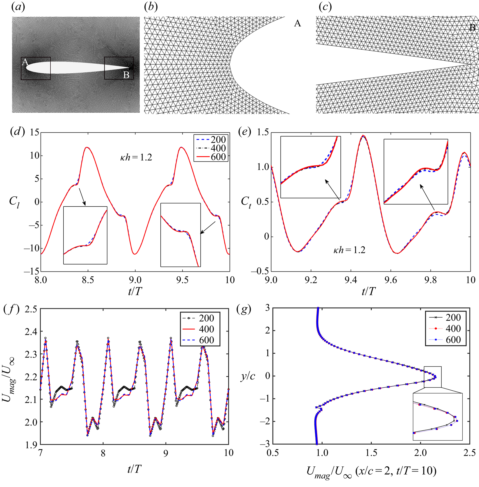
Figure 3. (a) Close-up view of the computational grid around the airfoil; zoomed view of the mesh around (b) the leading-edge (inset ‘A’) and (c) the trailing-edge (inset ‘B’); grid independence results for (d)  $C_l$, (e) $C_t$; (f) instantaneous velocity time-history at $x/c = 2, y/c = 0$; and (g) instantaneous velocity profile at $x/c = 2, t/T = 10$. The legends in panels (d–g) indicate the number of points on the airfoil surface.
Table 1. Results of grid independence study (% relative error). The abbreviation RMS stands for root mean square.

2.4. Validation of the solver
The unsteady flow solver has been extensively validated both qualitatively and quantitatively for pure heaving as well as pure pitching kinematics by comparing the results of present computations with experimental studies available in the literature – see Bose & Sarkar (Reference Bose and Sarkar2018). Figure 4 presents the qualitative validation of the flow solver in terms of a comparison of the trailing-edge wake patterns of a heaving airfoil obtained from the present computations with results from the dye flow visualization available in Jones et al. (Reference Jones, Dohring and Platzer1998) for two different  $\kappa h$ values. Figures 4(a) and 4(b) show the comparison of wake vorticity contours for $\kappa =3$ and $h=0.2$ ( $\kappa h=0.60$). The present computational results corroborate the experimental results in capturing the reverse Kármán vortex street. A similar comparison is presented for a higher non-dimensional heave velocity case for $\kappa =12.5$ and $h=0.12$ ( $\kappa h = 1.50$) in figures 4(c) and 4(d). A deflected vortex street is observed for such high non-dimensional heave velocities ( $\kappa h>1.00$). A close agreement is seen between the computational and experimental flow patterns in this case, as well.

Figure 4. A comparison of the vorticity contours from the present computation (a,c) with the dye flow visualization results obtained by Jones et al. (Reference Jones, Dohring and Platzer1998) (b,d) for a heaving airfoil with kinematic parameters:  $\kappa h=0.60$, $h=0.20$ (a,b) and $\kappa h=1.50$, $h=0.12$ (c,d). (Permission to reproduce the experimental frames has been obtained from the authors.)
The present solver has also been qualitatively validated in the periodic as well as the chaotic regime in terms of phase-averaged vorticity fields, by comparing with the two-dimensional experimental results of Lentink et al. (Reference Lentink, Van Heijst, Muijres and Van Leeuwen2010) – see figure 5. The comparison for the chaotic case is presented close to the onset of chaos at  $\kappa h = 2.1$, with the experimental result that is available nearest to the onset. The phase-averaged vorticity fields from the experimental results of Lentink et al. (Reference Lentink, Van Heijst, Muijres and Van Leeuwen2010) are shown in figures 5(a) and 5(b), respectively. For the numerical simulations, the phase-averaged vorticity contours are obtained by averaging the flow field snapshots over the same time interval and presented in figures 5(c) and 5(d), corresponding to $\kappa h = 1.25$ and $2.1$, respectively. A crisp pattern, as observed in figures 5(a) and 5(c) for $\kappa h = 1.25$ (with $\alpha _0 = 0^\circ$), results due to repeating flow-structures in the consecutive cycles, and thus is representative of periodic dynamics. On the other hand, a blurry pattern is observed for $\kappa h$ = 2.1 (with $\alpha _0 = 15^\circ$) in figures 5(b) and 5(d), indicating loss of periodicity due to unpredictable chaotic interactions in the wake. The phase-averaged vorticity field for $\kappa h = 2.5$ (with $\alpha _0 = 15^\circ$) also shows a qualitatively similar blurry pattern, representative of chaos (not shown here for the sake of brevity). The numerical predictions are seen to match the experimental results qualitatively, having a reasonable agreement on the onset of aperiodicity as well. Nevertheless, a direct one-to-one comparison cannot be made here since the experiments were carried out with an elliptic airfoil, having 5 % relative thickness. Note that both the studies are carried out at $Re = 10^3$.

Figure 5. Phase-averaged vorticity contours at different non-dimensional heaving velocities ( $kh$). Images in panels (a,b) are from the soap film experiments by Lentink et al. (Reference Lentink, Van Heijst, Muijres and Van Leeuwen2010). Images in panels (c,d) are results from the present computations. The experimental parameters are (a) $\kappa = 1.25$, $h = 1$, $\kappa h = 1.25$, $\alpha _0 = 0^\circ$; (b) $\kappa = 2.094$, $h = 1$, $\kappa h = 2.094$, $\alpha _0 = 15^\circ$. The present simulation parameters are (c) $\kappa = 1.25$, $h = 1$, $\kappa h = 1.25$, $\alpha _0 = 0^\circ$; (d) $\kappa = 2$, $h = 1.05$, $\kappa h = 2.1$, $\alpha _0 = 15^\circ$ (Permission has been obtained to reproduce the experimental results from the publishers of the original work).
A quantitative validation study has been performed for a pure heaving case for high values of  $\kappa h$ (up to $\kappa h \sim 1.9$), where the drag coefficient ( $C_d$) has been compared with the experimental measurements of Cleaver, Wang & Gursul (Reference Cleaver, Wang and Gursul2012) at $Re = 10\,000$ – see figure 6(a). Additionally, a combined pitching–heaving kinematics case has also been used for quantitative validation, by comparing with the thrust coefficients from the recent experimental results of Van Buren et al. (Reference Van Buren, Floryan and Smits2019). The authors carried out experimental force measurements for a teardrop airfoil for various amplitudes and frequencies in a water tunnel at $Re = 8000$. Figure 6(b) shows the comparison of the time-averaged thrust coefficients for different non-dimensional frequencies $f^*$ ( ${=}fc/U_\infty$), for $\alpha _0 = 15^{\circ }$ and $h=0.25$ ( $h_0 = 20 \ \mathrm {mm}$). The present computational results show very good agreement with the experimental results for both the cases.

Figure 6. (a) Comparison of drag coefficient ( $C_d$) with the experimental measurements of Cleaver et al. (Reference Cleaver, Wang and Gursul2012) for a heaving airfoil at $Re = 1 \times 10^4$; (b) comparison of time-averaged thrust coefficients ( $\bar {C}_T$) with the experimental measurements of Van Buren et al. (Reference Van Buren, Floryan and Smits2019) for a simultaneously pitching–heaving airfoil with $\alpha _0 = 15^{\circ }$, $h = 0.25 \ (h_0 = 20 \ \mathrm {mm})$, $Re = 8\times 10^3$.
3. Course of dynamical transition in the overall wake pattern
The parametric variation of  $\kappa h$ has been planned in the present study in such a way that the transition of the trailing wake from periodic reverse Kármán to chaos can be captured. We analyse the overall behaviour in terms of the near- and far-field wakes. The near-field is defined as the region that mainly includes the leading-edge separation and where the interactions between the primary LEV and trailing-edge vortices (TEVs) take place giving rise to the primary vortex couple at the trailing edge (also referred to as the ‘immediate vortex couple’ in this paper). The rest of the downstream region is termed as the far-field or far-wake. These two regions are schematically shown in figure 7. In our recent work (Bose & Sarkar Reference Bose and Sarkar2018), a quasi-periodic route to chaos was identified in the near-field of a simultaneously pitching–heaving system. This transition route is revisited here with a fresh perspective of interlinking the near-and far-wake behaviour. In order to do so, the parametric variation of $\kappa h$ has been considered with a finer resolution in the present study as compared with Bose & Sarkar (Reference Bose and Sarkar2018). The periodicity in the near-field is lost as $h$ is gradually increased beyond $0.80$ ( $\kappa h \geqslant 1.60$), giving way to a quasi-periodic transition. The quasi-periodic state, upon increasing $h$ further, gives rise to the dynamical state of intermittency in which multiple windows of aperiodic (chaotic) bursts appear in the otherwise quasi-periodic state. The bursts become more frequent with increasing $h$ and the dynamics ultimately culminates into chaos beyond a threshold value of $\kappa h$. Intermittency is a stable dynamical state but could not be captured by Bose & Sarkar (Reference Bose and Sarkar2018) as an extremely fine resolution of parametric variation is required in order to capture it, which is considered in the present study. Consequently, a more detailed transition route to chaos is presented here. The near-field behaviour gets directly reflected on the aerodynamic loads. Hence, the load time histories are chosen to analyse the near-field dynamics in detail. As will be presented later in the paper, a dynamic interlinking of the near- and far-field behaviour can reveal that intermittency in the near-field successfully explains the interesting transitional wake patterns observed in the far-field. Note that no investigation on the far-field behaviour was taken up by Bose & Sarkar (Reference Bose and Sarkar2018). In this section, the existence of four distinct dynamical states (periodic, quasi-periodic, intermittent and chaotic) is conclusively established through nonlinear time series analyses of the drag coefficient ( $C_d$) using an array of tools based on dynamical systems theories, such as, phase portraits, frequency spectra, time-frequency analyses (wavelet spectra) and recurrence plots (RPs). The same dynamics is also observed in the lift coefficient ( $C_l$) time histories, but are not presented here for the sake of brevity.
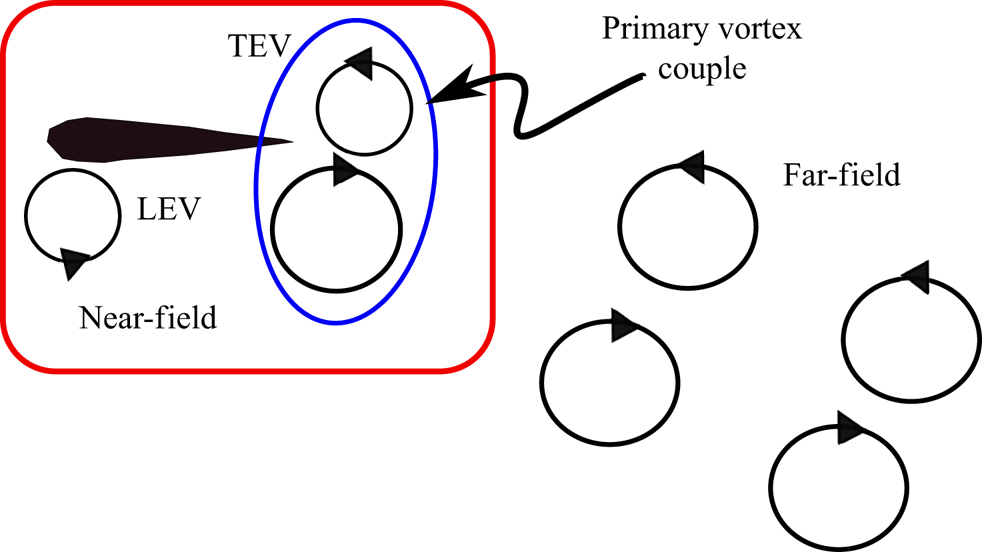
Figure 7. Schematic representation of near- and far-field wake regions.
The associated far-field behaviour and the role of the near-field interactions in shaping the far-wake dynamics is the main focus of discussion in the present section. At low  $\kappa h$ values ( $\kappa h < 1.5$), the entire flow field remains periodic. Vortex interactions in the near-field happens in a regular fashion that result in a reverse Kármán vortex street which subsequently becomes a stable deflected reverse Kármán wake. During the quasi-periodic transition in the near-field, this deflected vortex street loses its stability in which its spatial pattern is lost and switching starts from the far end of the wake. This dynamical state is followed by a regime of intermittency in the near wake, where bursts of aperiodic interactions in the near-field makes the wake experience switching that happens at the trailing edge intermittently. As the intermittent aperiodic windows appear more and more frequently, switching becomes more rampant and repeats in an aperiodic manner. Eventually, the structure of the immediate vortex couple at the trailing-edge, responsible for promoting an organized wake, is destroyed completely paving way to sustained chaos in both near- and far-fields. In this section, the actual triggers in the flow field for the above-mentioned transitions are identified, and also a connection between the near- and far-field wake dynamics is established.
Note that the qualitative flow field and the wake patterns across all the different dynamical states discussed in this paper are presented in terms of vorticity contours. The vorticity range has now been kept uniform as  $-10$ to 10 for all the presented vorticity contours in this paper. However, for certain cases, the LCS are also presented to augment the discussion. For example, the wake interactions become quite complicated at high $\kappa h$ values as the flow field loses periodicity, identifying LCS (Haller & Yuan Reference Haller and Yuan2000; Haller Reference Haller2015) enables better understanding about the flow physics to be achieved in these cases, through a better visualization of the vortex structures. Hence, the LCSs are tracked along with the vorticity contours for the important snapshots of the flow field in different dynamical regimes to capture the intricate details of the wake patterns and the underlying vortex interactions. Lagrangian coherent structures are identified in terms of the bFTLE (Haller Reference Haller2001) ridges. A finite-time Lyapunov exponent (FTLE) range of 0 to 0.5 is used for all bFTLE contours. The bFTLE ridges represent the attracting material lines in the unsteady flow field and are characteristic of the unstable manifolds (dynamic transport barriers in the flow) that contain the information of the past. Here, the bFTLE ridges are computed based on the Cauchy–Green tensor of the velocity vector field using the algorithm developed by Onu, Huhn & Haller (Reference Onu, Huhn and Haller2015). The attracting bFTLE contours help in understanding the complex vortex interactions, especially in the aperiodic regime, with better clarity as compared with the vorticity contours. Discussions in the following subsections are presented for different $\kappa h$ values corresponding to different dynamical states highlighting the respective behaviour of the near and far-fields.
3.1.  $\kappa h = 1.00$ and 1.40: periodic near-field and deflected reverse Kármán wakes

Figure 8(a) presents the time history of  $C_d$ at $h =0.50$ ( $\kappa h = 1.00$) which shows a constant amplitude regular oscillatory behaviour indicative of periodic dynamics in the near-field. In order to reveal the system attractors, the pseudo-phase-portraits are reconstructed from the scalar time series of $C_d$. The time-delay reconstruction of the pseudo-phase-space is performed using Takens’ embedding theorem (Takens Reference Takens1981). The method of time delay involves obtaining a series of independent time-delayed vectors representing the system dynamics from a single time series data based on an optimum time delay (say $\tau$) and the minimum embedding dimension (say $m$) of the system. The reconstruction matrix ( $Y$) can be expressed as $Y = [C_d(t)\ C_d(t+\tau )\ C_d(t+2\tau )\ldots C_d(t+(m-1)\tau )]$. The value of $\tau$ is determined using the method of mutual information (Fraser & Swinney Reference Fraser and Swinney1986) by calculating the average mutual information between the original and the time delayed vectors. The required value of $m$ is computed using the method of false neighbourhood (Kennel, Brown & Abarbanel Reference Kennel, Brown and Abarbanel1992) by checking whether the distance between two points in the phase space is invariant with increasing dimension. Time series analysis has been carried out on sufficiently long-time simulations (approximately 80 flapping cycles) to establish the correct dynamical state, the first 10 cycles of which have been neglected to ensure that the cycles with transient effects are not included in the analysis. The reconstructed phase portrait at $h = 0.50$ (figure 8b) represents a closed one-dimensional attractor characterizing the periodic nature of the dynamics. The corresponding frequency spectra consists of a dominant frequency $f1$ (double the flapping frequency) and its superharmonics (see figure 8c), thus confirming the periodic state.
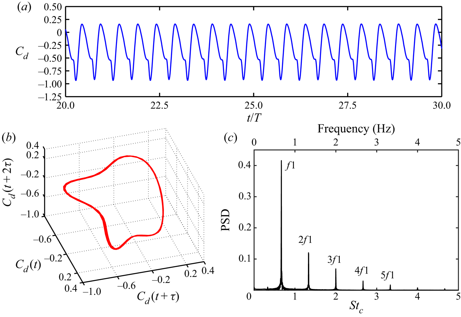
Figure 8. Time series analyses of  $C_d$ at $\kappa h = 1.00$ for the periodic regime: (a) time history; (b) phase portrait; (c) frequency spectra.
In the corresponding flow field, the periodic vortex interactions in the near-field results in a reverse Kármán street. It is an outcome of the alternate shedding of isolated vortices with opposite sense of rotation in every half-cycle. The corresponding vorticity and bFTLE contours are shown in figures 9(a) and 9(b), respectively. Note that a reverse Kármán wake is a signature of thrust generation by the flapping foil with zero mean lift. With increase in  $\kappa h$, the spatial symmetry of the reverse Kármán wake is lost giving rise to a deflected reverse Kármán wake at $h = 0.70$ ( $\kappa h = 1.40$). In the present case, the deflection is observed in the downward direction – see the corresponding vorticity and bFTLE contours in figures 9(c) and 9(d), respectively. The deflected wake remains stable at the far-field (confirmed through a sufficiently long time history of the simulation) in this dynamical state. It must be noted that a secondary vortex street is also formed at the same time, and is deflected in the upward direction. It consists of a series of clockwise (CW) vortices of much weaker strengths compared with those in the downward deflected primary vortex street (see figure 9d). Note that the dynamical signature of the deflected reverse Kármán wake is also periodic at $\kappa h = 1.40$. The time scales related to the secondary vortex-street are ascribed to the superharmonics of the shedding frequency of the immediate vortex couple, which is same as the flapping frequency.

Figure 9. Wake characteristics in the periodic regime: (a,b) symmetric reverse BvK wake at  $\kappa h = 1.00$; (c,d) asymmetric deflected wake at $\kappa h = 1.40$. The present colourmap of vorticity contours (with a range of $-10$ to 10) has been used in the rest of the paper. (a) Vorticity contour at $t/T = 60$; (b) LCS (bFTLE contours) at $t/T = 60$; (c) vorticity contour at $t/T = 60$; (d) LCS (bFTLE contours) at $t/T = 60$.
3.2. $\kappa h = 1.60$: quasi-periodic near-field and switching of deflection direction at the far end of the wake

With further increase in  $h$, the near-field is seen to attain a quasi-periodic state through small phase lags in the leading-edge separation behaviour from one cycle to another. Time history of $C_d$ showing a modulating oscillation at $h =0.80$ ( $\kappa h =1.60$) is indicative of quasi-periodic behaviour and is in contrast to the previous periodic case – see figure 10(a). The corresponding reconstructed pseudo-phase-portrait takes a toroidal shape (figure 10b) which is indicative of a quasi-periodic attractor. Besides, the presence of two incommensurate frequencies ( $f1$ and $f2$) along with the presence of other non-harmonic frequencies, that are in linear combinations of these two, further establishes the existence of a quasi-periodic dynamics – see figure 10(c).

Figure 10. Time series analyses of  $C_d$ at $\kappa h = 1.60$ for the quasi-periodic regime: (a) time history; (b) phase portrait; (c) frequency spectra.
In this parametric regime, the wake that remained deflected downwards during the periodic regime gradually begins to lose its downward structure at its far end during the 15th flapping cycle. The vorticity contours, presented in figure 11, show the corresponding wake patterns at different flapping cycles. Initially, the wake is deflected completely downward (figure 11a) until at the 15th cycle a switch in its deflection direction is noticed at the far end of the wake (see figure 11b). The vortex street still remains deflected downward near the trailing-edge and as a result, it takes an arc-like shape. To understand this transition better, the individual motion paths of three consecutive trailing-edge couples, namely the  $C_{13}$, $C_{14}$ and $C_{15}$ which are formed at the start of the $13\textrm {th}$, $14\textrm {th}$ and $15\textrm {th}$ cycles, respectively, are tracked – see figure 12. It is seen that $C_{13}$ follows a straight downward deflected path until it gets dissipated in the far-field; $C_{14}$ initially traverses in the downward direction but gradually switches its direction at the far end of the wake during the $15\textrm {th}$ cycle; $C_{15}$ undergoes a similar switching behaviour. However, the latter's path is different with a higher upward deflection angle compared with $C_{14}$ at the far end. The subsequent primary couples continue to switch the deflection direction in a similar fashion at the far end but with small deviations in their upward deflection angles. After that, the wake remains stable in its switched state with an arc shape and no further switch in the deflection direction is observed. This has been confirmed by running the simulations through long time windows (carried out until $t/T = 70$). The overall mechanism of the formation of the immediate vortex couple at the trailing-edge remains very similar in each cycle with only minor deviations. These deviations are the result of small phase lags in the separation behaviour of the LEVs and the subsequent near-field interactions, from one cycle to another, that show up as quasi-periodic dynamics in the near-field behaviour and the load patterns. The detailed analysis of the emergence of quasi-periodic trigger and the underlying role of LEV was discussed in Bose & Sarkar (Reference Bose and Sarkar2018).

Figure 11. The change in the deflection pattern of a downward deflected wake at the far end of the wake during different flapping cycles at  $\kappa h = 1.60$ with $t/T =10, 15, 20, 25, 30, 35, 40, 45, 50$ in panels (a–i), respectively.

Figure 12. Comparison of motion trajectories of three consecutive primary vortex couples ( $C_{13}$, $C_{14}$ and $C_{15}$) during far-end switching of the wake at $\kappa h = 1.60$.
As a result, the arc-shaped wake shows minor deviation from one cycle to another, and the wakes stay in each other's neighbourhood – see figure 13(a–h). A superposition of the centrelines of the wake for different flapping cycles ( $15\textrm {th}\text {--}50\textrm {th}$), shown in figure 13(i), reveals that the path line of these couples are not unique and the upward deflection angle of the vortex street in the far-end changes slightly from one cycle to another. This highlights the quasi-periodic tendency present in the wake deflection behaviour.

Figure 13. (a–h) The shape of the wake at  $\kappa h = 1.60$ for different flapping cycles ( $15\textrm {th}\text {--}50\textrm {th}$); (i) superposition of the centrelines of the spatial shapes of the wake for different flapping cycles ( $15\textrm {th}\text {--}50\textrm {th}$) at $\kappa h = 1.60$ showing the quasi-periodic signature.
Figures 14(a) and 14(b) present the LCS (in terms of bFTLE contours) of the deflected patterns before and after the far-end switching, respectively. Note that an organized secondary vortex street consisting of a series of CW vortex pairs is observed, while the primary wake is deflected downward – this is shown at  $t/T = 10$, in figure 14(a). Minor deviations in the near-field interactions between the LEV and the TEV, owing to quasi-periodicity, are seen to propagate through the secondary vortex street in terms of a phase lag in the formation of consecutive vortex pairs. For a better understanding, one such typical sequence of interactions is presented in figure 15. Although the far-wake switching (FWS) is first observed in the 15th cycle, the gradual propagation of the underlying quasi-periodic trigger starts at an earlier flapping cycle, hence, the chronology of vortex interactions during the 12th cycle is presented in figure 15. The quasi-periodic trigger, that emerged from the leading-edge shedding and the subsequent LEV–TEV interactions, gets propagated in the far-wake through the forward motion of the immediate vortex couple, as well as through a series of interactions among the secondary vortex structures generated in the near-field. As the immediate vortex couple $\boldsymbol {C}'$ moves forward with the free stream, the trailing-edge vortex filament entailed with the vortex couple gets strained and eventually gets split into small isolated CW vortices – SV1 and SV2 – in the near-wake due to the stronger CW counterparts of $\boldsymbol {C}'$ – see figure 15(b,c). As can be seen from figure 15(c), the motion of SV1 is initially governed by the resultant velocity induced by the previously existing same-sense secondary vortex SV0, as well as the opposite-sense TEV, and is inversely proportional to their corresponding normal distances $r1$ and $r2$, respectively. The opposite-sense TEV tries to form a couple with SV1, whereas, same-sense SV0 applies a CW rotational velocity on it. Subsequently, another LEV is shed as a vortex couple $\boldsymbol {C}''$, which becomes another influencing factor. The anticlockwise (ACW) component of $\boldsymbol {C}''$ undergoes a partial merging with the TEV and the CW counterpart interacts with SV1 – see figure 15(f). Eventually, SV1 moves with its resultant velocity and participate in forming the secondary vortex street with the existing array of CW vortex pairs. Therefore, the formation of the secondary vortex street indirectly depends on the LEV–TEV interactions. It is worthwhile to mention that this chronology of events changes by a small margin in every flapping cycle due to quasi-periodicity, which in turn changes the resultant velocity of the secondary vortices. Consequently, a phase lag is induced in the formation of subsequent vortex pairs, which eventually results in multiple merging among the vortex pairs in the secondary vortex-street. This leads to a gradual destruction of the secondary vortex-street, which can be seen from the sequence of interactions during 10 consecutive cycles from $t/T = 10$ to $t/T = 20$, presented in figure 16. As a result, a region of disturbance is created in the far end of the wake that influences the vortex couples to switch their deflection direction in that region. This can be considered as one of the mechanisms of FWS.

Figure 14. The bFTLE contours at  $\kappa h = 1.60$ with (a) $t/T = 10$, (b) $t/T = 20$. The colourmap of bFTLE contour is same as that of figure 9.

Figure 15. A typical sequence of near-field interactions in the 12th cycle affecting the formation of a CW vortex pair in the secondary vortex street.

Figure 16. Transition in the secondary vortex street at  $\kappa h = 1.60$. Here $t/T = 10, 11, 12, 13, 14, 15, 16, 17, 18, 19, 20$ in panels (a–k), respectively.
Wei & Zheng (Reference Wei and Zheng2014) also observed a similar far-end switching for a heaving airfoil at a regime of high reduced frequency ( $k = 20$) and a small amplitude ( $h = 0.06$). However, the quasi-periodic signature of the switching phenomenon and the presence of the secondary vortex street and the associated transitions were not observed by the authors. A vortex interaction mechanism in the far-wake, termed as ‘opposite vortex pairing process’, characterized by exchange of partners among consecutive couples, was said to be responsible for the far-end switching. The authors further reported that, as the distance between consecutive couples decreases while the distance between the opposite sense partners in each couple increases, a more favourable condition for this mechanism to take place is created. However, this observation seems to be applicable only for the high frequency and low amplitude cases where the distance between couples are less, and wake formation is primarily a trailing-edge phenomenon without much contribution from the LEVs. In fact, well-formed LEVs are either absent (Wei & Zheng Reference Wei and Zheng2014; Shinde & Arakeri Reference Shinde and Arakeri2013) or are mostly dissipated by their interactions with the subsequent nascent LEVs (Lewin & Haj-Hariri Reference Lewin and Haj-Hariri2003) for these high frequency and low amplitude cases. The present study does not fall under this parametric range and no such opposite vortex pairing process has been observed here. Rather, the primary trigger for the far-end switching comes from the minor deviations in the quasi-periodic near-field interactions between the LEV and the TEV that is propagated through the transition in the secondary vortex street. To the best of the authors’ knowledge, this kind of quasi-periodic switching in the wake of a pitching–heaving system is being reported for the first time in the present study.
3.3. $\kappa h$ = 1.66: appearance of intermittency and switching of the immediate vortex couple

As the value of  $h$ is further increased to $h = 0.83$ ( $\kappa h = 1.66$), the quasi-periodic signature starts to get interspersed with irregular windows of chaos. Such temporal patterns of response are reported as intermittency in the nonlinear dynamics literature (Hilborn Reference Hilborn2000), in which the system irregularly switches between two different attractors or dynamical states. In this case, the switch happens between the state of quasi-periodicity and chaos. The sporadic bursts of aperiodic windows are expected to become longer as the parameter value ( $h$) increases gradually. The intermittent aperiodic windows appear due to the stronger perturbations coming from the leading-edge separation resulting in nonlinear interactions among the near-field flow-structures. The time history of $C_d$ at $h = 0.83$, presented in figure 17(a), shows a typical intermittent state where the insets ‘A1’, ‘B1’, ‘C1’ and ‘D1’ denote the sporadic aperiodic windows. A better understanding of the temporal evolution of the frequency content is possible from the scalogram obtained through the wavelet analysis using the Morlet wavelet function (Grossmann, Kronland-Martinet & Morlet Reference Grossmann, Kronland-Martinet and Morlet1990) – see figure 17(b). Sporadic bursts of broadband frequencies that correspond to the aperiodic windows are clearly seen from the wavelet spectra – see inlet sections ‘A1’, ‘B1’, ‘C1’ and ‘D1’ in figure 17(b). The time history and the wavelet spectra of $C_d$ at a higher $h$ of 0.85 ( $\kappa h = 1.70$), presented in figures 17(c) and 17(d), respectively, show that such aperiodic windows (‘A2’, ‘B2’, ‘C2’ and ‘D2’ in this case) are significantly longer and more frequent than that of the previous case ( $h =0.83$). As $h$ increases further and reaches a threshold, the entire time window turns aperiodic and the response becomes completely chaotic.

Figure 17. Time series analyses of  $C_d$ at $\kappa h = 1.66$ and $\kappa h = 1.70$: intermittent dynamics; the aperiodic window is marked as ‘Z’. (a) Time history of drag coefficient ( $C_d$) at $\kappa h = 1.66$. (b) Wavelet spectra of drag coefficient ( $C_d$) at $\kappa h = 1.66$. (c) Time history of drag coefficient ( $C_d$) at $\kappa h = 1.70$. (d) Wavelet spectra of drag coefficient ( $C_d$) at $\kappa h = 1.70$. (e) Phase portrait of $C_d$ at $\kappa h = 1.70$. (f) Frequency spectra of $C_d$ at $\kappa h = 1.70$.
The reconstructed pseudo-phase-portraits and the frequency spectra for the intermittent state at  $h = 0.85$ ( $\kappa h = 1.70$) are presented in figures 17(e) and 17(f), respectively. The appearance of small regions of aperiodic evolution of the trajectory in the otherwise toroidal phase portrait is clear. However, these characteristics of intermittency are not captured in the frequency spectra as it reflects an average quasi-periodic behaviour of the system. The existence of intermittency can be conclusively established using RPs (Eckmann & Ruelle Reference Eckmann and Ruelle1985; Marwan et al. Reference Marwan, Carmen Romano, Thiel and Kurths2007). The changes in the dynamical signature of a system are revealed very easily through the visual representation of RPs. Also, RPs bring out meaningful results even from relatively short time data unlike the conventional time series tools which require sufficiently long time histories for the convergence of the respective algorithms. Recurrence plots are constructed from a binary recurrence matrix, $R_{i,j} = \varTheta (\epsilon - ||x_i -x_j||); i,j = 1,2,3..N$, for a phase space with $N$ points. Here, $x_i$ is a point in the ‘ $d$’-dimensional phase space, $\varTheta$ is the Heaviside step function, $\epsilon$ is a predefined threshold and $||\cdot ||$ indicates the $L_2$ norm. The graphical representation of RPs are sensitive to the threshold $\epsilon$; an optimal value of $\epsilon$ needs to be chosen to represent the dynamics accurately. In the present calculations, $\epsilon$ is chosen to be 10 % of the diameter of the reconstructed phase space. The diameter refers to the distance between the two farthest points in the phase space. $R_{i,j}$ is considered to be zero if the distance between the two points $x_i$ and $x_j$ in the phase space is greater than $\epsilon$, or else it is equal to unity. The RP contains black and white points corresponding to the ones and zeros of the recurrence matrix, respectively. The RP for the $C_d$ time history at $h = 0.85$ ( $\kappa h = 1.70$) is presented in figure 18, which clearly reflects the intermittent transition through alternative windows with different characteristics over the main diagonal. There are sporadic aperiodic windows over the main diagonal (one such is marked as ‘Z’) consisting of mostly small broken lines. This is indicative of the non-recurrent signature corresponding to the aperiodic dynamics and is in contrast to the periodic signature, which comprises of equidistant solid diagonal lines parallel to the primary diagonal.

Figure 18. RP of  $C_d$ at $\kappa h = 1.70$.
The most important outcome of intermittency on the flow field is the switching of the immediate vortex couple at the trailing-edge which is triggered by the aperiodic bursts. During these bursts, the wake goes through an aperiodic breakdown resulting in spontaneous and arbitrary movements of vortex couples in different directions before reorganizing itself into a fully deflected pattern of the opposite direction. As discussed before, in the quasi-periodic state ( $\kappa h = 1.60$), the near-field disturbances are propagated mainly through the secondary vortex street in terms of minor deviations in its pairing process and these disturbances deflect the wake at its far end giving it an arc shape. The intermittent transition does not, however, follow the same mechanism. Instead, the aperiodic interactions during the intermittent chaotic bursts provide quick and strong disturbance at the region immediately close to the body (trailing-edge) which flips the deflection direction of the immediate couple. This eventually makes the whole wake follow the same flipped direction and a fully reversed (upward or downward) wake is obtained. However, when the aperiodic window ends, far-end switching slowly starts to take place after experiencing the expected quasi-periodic trigger from the near-field giving rise to an arc-shaped wake. The next aperiodic burst flips the immediate couple again and the whole wake follows that signature and thus the process continues. To summarize, four different wake patterns are observed at different flapping cycles in the dynamical state of intermittency – see figure 19. Figure 19(a) is indicative of a downward deflected wake pattern ${D}$ at $t/T = 30$. A concave and a convex arc-shaped far-wake switched wake – FWS DU and FWS UD – are observed at $t/T = 32$ and $65$, respectively; see figures 19(b) and 19(c). Figures 19(d) and 19(e) present an aperiodic ${A}$ and an upward deflected ${U}$ wake pattern, respectively, at $t/T = 35$ and $42$. Therefore, the jet-switching phenomenon does not take place directly from the ${D}$ to the ${U}$ wake and vice versa, rather, it is associated with different intermediate transitional wake patterns (FWS and ${A}$). For example, a ${D}$ wake undergoes a complete reversal of its deflection direction that results in a ${U}$ wake, after evolving through FWS DU and ${A}$ wakes in the process. Subsequently, the ${U}$ wake transitions back to a ${D}$ wake through the sequence of FWS UD and ${A}$ patterns.

Figure 19. Vorticity contours corresponding to different transitional wake patterns at  $\kappa h = 1.66$: (a) downward deflected ( ${D}$); (b) far-wake switched downward at the near-field and upward at the far-field (FWS-DU); (c) aperiodic ( ${A}$); (d) upward deflected ( ${U}$) and (e) far-wake switched upward at the near-field and downward at the far-field (FWS-UD). Here $t/T = 30, 32, 35, 42, 65$ in panels (a–e), respectively.
Figure 20 connects the spatial transitions that take place in the far-wake in terms of the occurrence of these four wake-patterns. The figure shows that the direction flipping of the immediate couple, accompanied by intermediate FWS and  ${A}$ wake patterns, happens in an irregular fashion. This observation is in contrast with Heathcote & Gursul (Reference Heathcote and Gursul2007) who reported a quasi-periodic pattern in their observed gradual switching of the deflected jet. Note that Heathcote & Gursul (Reference Heathcote and Gursul2007) only reported ${D}$ and ${U}$ wakes and transitions between them. Far-wake switching was not observed in their study. Moreover, the authors did not analyse this immediate couple switching phenomenon from a dynamical perspective either, as has been carried out in the present study with an objective of establishing the overall transition route. It is also observed that FWS wakes can evolve into ${A}$ patterns during the aperiodic bursts, only if the aperiodic window is long enough to flip the immediate couple. One such window is marked as ‘C1’ in the drag time-history in figure 17(a). In this case, the organization of the entire wake breaks down to an ${A}$ pattern (figure 19c) before reorganizing itself into the ${U}$ wake (figure 19d). Conversely, the immediate couple switching may not take place if the aperiodic bursts are short, such as ‘A1’ (around $t/T = 15$), ‘B1’ (around $t/T = 22$) or ‘D1’ (around $t/T = 48$) as marked in figure 17(a). In these cases, the aperiodic perturbations in the near-field are not sufficiently strong due to their short presence to flip the immediate couple and the wake regains the FWS pattern after a small windows of aperiodicity ( ${A}$) – see figure 20.

Figure 20. Different transitional wake patterns versus number of flapping cycles:  ${U}$, upward deflected, ${A}$, aperiodic and ${D}$, downward deflected. The numbers over the boxes denote the duration in terms of the number of flapping cycles ( $\kappa h = 1.66$); ‘A1’, ‘B1’, ‘C1’, ‘D1’ are windows of aperiodic bursts as marked in figure 17(a).
To understand how the  ${A}$ pattern kicks in, the motion paths of the immediate couples are followed between $t/T = 32$ to $t/T = 35$, where the wake follows an FWS pattern just before the start of aperiodic window ‘C1’. The main vortex couples are $C_{32}$, $C_{33}$, $C_{34}$ and $C_{35}$, formed as the immediate couples at the start of $32\mathrm {nd}$, $33\mathrm {rd}$, $34\mathrm {th}$ and $35\mathrm {th}$ cycles, respectively. The vortex couple $C_{32}$ initially follows a downward path in the $32\mathrm {nd}$ cycle, however, gradually switching upwards in the far end (at approximately $9c$ from the trailing-edge) during the $33\mathrm {rd}$ cycle – see figure 21. The upward deflection angle is seen to be small in this case. The vortex couple $C_{33}$ also undergoes a similar upward switching in the far-field, but at a relatively closer distance from the trailing-edge (at approximately $5c$ from the trailing-edge) and the deflection angle is also higher. The vortex couple $C_{34}$ follows a downward deflected path throughout, which destroys the organization of the prevailing FWS pattern. The next couple $C_{35}$ undergoes an upward switching at the far end (at approximately $3c$ from the trailing-edge). This chain of events is presented here as an example of the transition of an FWS pattern, which is facilitated by the arbitrary movement of the primary couple at the start of the aperiodic burst. This is followed by the switching of the immediate couple in the subsequent cycles.

Figure 21. Comparison of motion trajectories of three consecutive primary vortex couples ( $C_{13}$, $C_{14}$ and $C_{15}$) during far-end switching of the wake at $\kappa h = 1.60$.
Figure 22(a–c) presents the LCSs of the  ${U}$, ${A}$ and ${D}$ wakes at $t/T = 30$, $35$ and $42$, respectively. The corresponding temporal as well as spatial evolution of the velocity profiles are presented in figure 23. Figures 23(a), 23(c) and 23(e) present the velocity contours during ${D}$ ( $t/T = 30$), ${A}$ ( $t/T = 35$) and ${U}$ ( $t/T = 42$) wake patterns, respectively. The spatial evolution of the velocity magnitude profiles (solid lines) and streamwise velocity profiles (dotted lines) corresponding to these three wake patterns are presented in figures 23(b), 23(d) and 23(f), respectively, for the strategic locations marked in the velocity contours. At $t/T = 30$, the locus of the maxima of the velocity profiles is seen to move downwards at the far-field, representing the ${D}$ wake. However, at $t/T =35$, the profiles get scattered as their distance from the trailing-edge increases. This characterizes the spatial aperiodicity in the ${A}$ wake. At $t/T = 42$, the locus of the maxima of the velocity profiles is seen to move upward. This shows the reorganization of the wake into a ${U}$ wake after the aperiodic burst. In order to show the temporal behaviour at a fixed spatial location, the velocity magnitude as well as the streamwise velocity profiles are plotted for five consecutive cycles from $t/T =34$ to $t/T = 38$ at $x/c = 7$ and are shown in figure 24. Despite having the same spatial location, both the profiles mark significant differences in their patterns from one cycle to another. This temporal behaviour of the flow field directly reflects the effect of the aperiodic time windows during the dynamical state of intermittency.

Figure 22. The bFTLE contours at  $\kappa h = 1.66$. Here (a) ${D}$ is the wake at $t/T = 30$; (b) the ${A}$ wake at $t/T = 35$; (c) the $\textbf {U}$ wake at $t/T = 42$. The colourmap of bFTLE contour is same as that of figure 9.

Figure 23. Vorticity contours and spatial evolution of velocity profiles during the regime of intermittency at  $\kappa h = 1.66$. In panels (b), (d) and (f) the solid lines refer to velocity magnitude profile and dotted lines refer to streamwise velocity profile. Panels (a–f) give the velocity contours at $t/T = 30, 30, 35, 35, 42, 42$, respectively.

Figure 24. Comparison of velocity magnitude (a) and streamwise velocity profiles (b) at  $x/c = 7$ in four consecutive cycles from $t/T = 34$ to $t/T =38$.
The direction flipping of the immediate couple becomes more frequent at higher  $\kappa h$ values as the frequency of aperiodic bursts increases. As a result, the far-wake does not get sufficient time to recover itself from the aperiodic state and eventually the whole wake becomes aperiodic. Similar increase in switching frequency was also reported by Heathcote & Gursul (Reference Heathcote and Gursul2007), for a pure heaving case. However, as mentioned earlier, the presence of FWS wakes or the underlying dynamical state of intermittency which brings out the varied wake patterns in the far-field was not observed in their study. The authors mentioned that this switching period of ${D}$ to ${U}$ to ${D}$ was observed to be two orders of magnitude higher than the heaving period. The present study shows that a full reversal from ${D}$ to ${U}$ (through FWS and ${A}$) can happen within 40 cycles. Figure 25(a) presents the variation of the period-averaged lift coefficients ( $\langle C_l\rangle$) over different flapping cycles. It is observed that its sign changes from negative to positive at approximately $t/T = 40$, indicating the switching of the immediate vortex couple from ${D}$ to ${U}$. Note that the dominant leading-edge separation at $Re=10^3$ for the present pitching–heaving case could be a possible reason for advancing the switching phenomenon, as compared with the experimental results of Heathcote & Gursul (Reference Heathcote and Gursul2007). It is also believed that the near-field disturbances accelerate the flipping of the immediate couple during the aperiodic bursts. Furthermore, the most probable states of the $C_l$ values are estimated through its probability distribution function (p.d.f.) and is presented in figure 25(b). Among the three dominant peaks, the peaks on either sides of $C_l = 0$ can, respectively, be attributed to the ${D}$ and ${U}$ modes of the wake in the pre- and post-jet-switching regime, confirming the bistability of the wake (Cadot, Evrard & Pastur Reference Cadot, Evrard and Pastur2015). The peak about zero primarily corresponds to the mean $C_l$ value.

Figure 25. (a) Variation of period-averaged lift coefficient ( $\langle C_l\rangle$); (b) p.d.f. of the instantaneous lift coefficient ( $C_l$).
3.4. $\kappa h = 2.50$: sustained chaos

As  $\kappa h$ is further increased ( $h \geqslant 1.00, \kappa h \geqslant 2.1$), the flow field attains a chaotic state through the frequent aperiodic windows. The $C_d$ time history is observed to be completely irregular at $h=1.25$ ( $\kappa h = 2.50$) – see figure 26(a). This chaotic state is represented by a volume in the state space with densely filled trajectories indicating the presence of a strange attractor in the phase space (figure 26b) and a broadband frequency spectrum (figure 26c). In this regime, the near-field interactions become significantly complex giving rise to spontaneous formation of fast-moving vortex couples. The free movement of the vortex couples and their collisions with other isolated vortices or other couples result in various fundamental vortex interactions (Leweke, Le Dizès & Williamson Reference Leweke, Le Dizès and Williamson2016) which eventually turn the flow field completely chaotic and sustain it. Rapid aperiodic jet-switching is seen to act as a precursor to the chaotic flow dynamics. Two typical snapshots of the vorticity contours and LCS corresponding to the chaotic flow topology at $t/T = 25$ and $t/T = 30$ are presented in figure 27. It is evident that there is no correlation between them as the flow field has become completely unpredictable in this regime.

Figure 26. Time series analyses of  $C_d$ time history at $\kappa h = 2.50$. (a) Time history; (b) phase portrait; (c) frequency spectra.

Figure 27. Chaotic flow topology at  $\kappa h = 2.50$. (a) Vorticity contour at $t/T = 12$; (b) bFTLE contours at $t/T = 12$; (c) vorticity contour at $t/T = 25$; (d) bFTLE contours at $t/T = 25$. The colourmap of bFTLE contour is same as that of figure 9.
The dynamical signature of the various transitional far-wake patterns during the jet-switching phenomenon has been conclusively established in this section. The intermittency in the near-field has been manifested to be the key reason behind the immediate couple switching at the trailing-edge for the first time. Finally, it has been substantiated that the aperiodic jet-switching acts as a precursor to sustained chaos in the flow field. The next section focuses on the underlying vortex interaction mechanisms through which these dynamical transitions, especially switching of the immediate couple at the trailing-edge takes place, leading to an eventual complete breakdown of the organization of the wake.
4. Mechanism of direction flipping of the immediate couple at the trailing-edge: role of LEV
The unsteady separation of LEVs is one of the governing factors that decides the nature of near-field interactions. It has been established that the first trigger to aperiodicity in the near-field emerges from the discrepancy of the leading-edge separation. The shedding frequency of the LEV becomes incommensurate to the flapping frequency and gives rise to the quasi-periodic trigger; refer to the supplementary data available at https://doi.org/10.1017/jfm.2020.1030 for the detailed analysis carried out to identify the source of quasi-periodicity. Subsequently, the diverse interactions among LEV, TEV and the other main near-field vortex structures propagate this aperiodic trigger, leading to qualitative changes in the dynamics of the wake. There exist a number of fundamental vortex interaction mechanisms in two dimensions, such as partial and complete merging, vortex splitting and shredding, collisions of vortex couples, exchange of partners, etc. that manifest the change in the flow dynamics. The detailed definitions of these mechanisms can be found in Leweke et al. (Reference Leweke, Le Dizès and Williamson2016). The LEV–TEV interactions lead to the formation of a strong vortex couple at the trailing-edge in every flapping cycle which becomes the primary unit of an organized wake. This section examines the near-field behaviour that is responsible for the flipping of this immediate couple in the intermittency regime ( $\kappa h = 1.66$), in terms of various fundamental vortex interactions; refer to ‘Movie1’ and ‘Movie2’ for the animated view of the underlying vortex interactions behind jet-switching and the role of LEV in triggering it, respectively. Detailed discussions are presented in the following to present the chronology of events that take place during the dynamical state of intermittency, in which a downward deflected couple at the trailing-edge can transition to an upward deflected couple through a window of aperiodic interactions. This phenomenon has been earlier referred to as the ‘direction flipping of the immediate couple’ in § 3.3.
All the flow field plots presented in this section belong to the regime of intermittency. The bFTLE contours for three consecutive flapping cycles (from  $33\mathrm {rd}$ to $35\mathrm {th}$) showing the near-field interactions are presented in figure 28. These cycles are chosen to demonstrate the change in the deflection direction of the immediate couple from downward to upward through an in-between aperiodic phase. The flapping cycles are presented from their up-strokes to down-strokes. During the up-stroke, the primary ACW LEV ‘1’ grows and subsequently forms couple ‘C2’ at the trailing-edge (figure 28a,c). At the same time, an ACW TEV ‘3’ sheds in the wake and two CW isolated vortices ‘4’ and ‘5’ are formed due to the rolling up of the trailing vortex filament from the primary couple of the previous cycle ‘C1’ (figure 28b). In the down-stroke, ‘C2’ traverses in an ACW circular arc and undergoes partial merging with ‘5’ and ‘3’, respectively (figure 28d,e). On the other hand, CW LEV ‘6’ and CW TEV ‘7’ shed and undergo partial merging to form an isolated CW vortex that interacts with the ACW component of ‘C2’ giving way to another primary vortex couple ‘C3’ (like ‘C1’) at the end of $33\mathrm {rd}$ cycle ( $t/T = 34$) (figure 28f). Note that ‘C3’ is deflected downwards at the trailing-edge.

Figure 28. Vortex interaction mechanisms during  $33\mathrm {rd}$ to $35\mathrm {th}$ cycles that underlie the immediate couple switching at $\kappa h = 1.66$. The present colourmap has also been used in figures 29 and 30.
During the up-stroke of the next cycle (35th), another ACW LEV ‘8’ grows, convects over the lower surface of the airfoil like ‘1’ (figure 28g–i). However, due to near-field disturbances, the location of its reattachment gets altered. A part of it is seen to circumnavigate the trailing-edge feeding the vortex filament connected with the TEV and the remaining part forms a weaker couple ‘C5’ (figure 28j). Therefore, the strength and the trajectory of this couple get significantly altered as compared with ‘C2’ of the previous cycle. Now ‘C5’ traverses in the ACW direction following a different circular arc with a significantly higher radius than that of ‘C2’ (figure 28k–m). As a result, ‘C5’ cannot come in the neighbourhood of the TEV shed in the next half-cycle as it did in the previous cycle, and the formation of the primary couple at the trailing-edge gets disrupted. Notably, the trigger comes from the discrepancy in the LEV separation which in turn alters the subsequent interactions in terms of the formation of ‘C5’. On the other hand, the ACW TEV ‘9’ sheds and forms couple ‘C4’ with the existing CW ‘5’ (figure 28i). Next ‘C4’ advects upwards due to its self-induced velocity and the connecting vortex filament splits into two ACW vortices ‘12’ and ‘13’ (figure 28j,k). At the same time, CW LEV ‘11’ evolves and convects over the upper surface and sheds from the trailing-edge (figure 28j–l). A CW TEV ‘14’ also sheds in the wake (figure 28l). The movements of these vortex structures are followed in the next cycle.
In the next cycle (35th), this aperiodic trigger is propagated further to the far-field through the self-induced movements of the generated vortex couples ‘C4’ and ‘C5’ and their subsequent interactions, thus destroying the organization of the wake. During the up-stroke, ‘11’ and ‘14’ undergo partial merging resulting in a CW isolated vortex ‘18’ (figure 28m–p). On the other hand, an ACW LEV ‘15’ grows, convects over the lower surface of the airfoil and sheds from the trailing-edge (figure 28m–o). Subsequently, it undergoes partial merging with the newly shed TEV and gains strength and forms an ACW vortex ‘17’ (figure 28p). Thus, the first couple of an upward deflected vortex street ‘C6’ is formed with ‘17’ and ‘18’ as the ACW and CW counterparts (figure 28p–r). The aperiodic window of near-field interactions ends by paving the way for an upward-deflected vortex couple through the flipping of its deflection direction at the trailing-edge. From the next cycle onwards, the primary vortex couple generated at the trailing-edge in every cycle is seen to have an upward self-induced velocity under the influence of ‘C6’ and the wake gradually starts to organize itself into the  ${U}$ pattern in the subsequent flapping cycles until the next transition happens. Until then (from $t/T =36$ up to $t/T = 40$), the far-wake remain disordered as an ‘A’ wake.
The detailed flow mechanism of formation of the upward deflected primary vortex couple during the 38th cycle is presented in figure 29. The ACW LEV ‘19’ forms a couple ‘C9’ with the CW secondary structure ‘20’ at the trailing-edge. The ACW component of ‘C9’ subsequently undergoes a partial merging with the same-signed TEV ‘21’ and the weaker CW counterpart gets eventually shredded, thus forming the ACW counterpart of the upward-deflected primary couple ‘C10’ (similar to ‘C7’). On the other hand, the CW component of the couple ‘C8’, formed from the contribution of the primary CW LEV and the secondary ACW vortex structure in the previous half-cycle, undergoes partial merging with the same-signed TEV and its ACW component eventually gets shredded. Thus, ‘C8’ gets transformed into a CW isolated vortex which constitutes the CW component of the primary couple ‘C10’.

Figure 29. Vortex interaction mechanism behind the formation of the upward deflected wake during 38th cycle.
As  $\kappa h$ increases, the frequency of such sporadic aperiodic bursts also increases resulting in more frequent switching of the immediate couple at the trailing-edge. As a result, the stay period of the wake in either of ${U}$ or ${D}$ patterns gradually decreases and eventually, the wake reaches a chaotic state ( $h \geqslant 1.00, \kappa h \geqslant 2.1, \alpha _0 = 15^\circ$) where the wake pattern becomes completely unpredictable and uncorrelated in the consecutive flapping cycles. In order to examine the implication of the leading-edge separation on the aperiodic transition during the dynamical state of chaos, the leading-edge behaviour at $h = 1.25$ is compared for three consecutive flapping cycles (11th to 13th) in figure 30. It is seen that the separation pattern gets significantly altered from one cycle to another. Thus, the aperiodic trigger can be attributed to this discrepancy in the leading-edge behaviour in the chaotic regime.

Figure 30. Comparison of the near-field flow-interactions in the three consecutive flapping cycles (11th–13th) in the chaotic regime at  $\kappa h = 2.50$.
Once the aperiodicity is triggered in the near-field by the irregular leading-edge separation, it starts to propagate downstream primarily through the near-field interactions resulting in spontaneous vortex couples irregularly moving in the upward and downward directions. The instantaneous bFTLE contours of the flow fields at  $h = 1.25$ during the 11th–13th cycles are presented in figure 31. Chaos is sustained in the far-field by these fast-moving couples and their subsequent inelastic collisions (Leweke et al. Reference Leweke, Le Dizès and Williamson2016) with other flow structures in the wake. As a result, the width of the wake increases significantly. It is noteworthy that the same chain of events is never seen to repeat in the consecutive cycles, making the flow patterns completely erratic in nature. The fundamental vortex interactions such as vortex merging, vortex splitting, vortex shredding, collision of couples, partner exchange (Leweke et al. Reference Leweke, Le Dizès and Williamson2016), are seen to occur spontaneously at different locations of the wake one after another in quick succession without having any regularity in their occurrence. It is important to note that the underlying vortex interactions in the near-field responsible for the switching of the immediate couple and the mechanism of jet-switching that have been discussed in the present section are important ingredients of the route to chaos in the far-field. Moreover, the present study uncovers the role of LEV in triggering the jet-switching phenomenon in the dynamical regime of intermittency. It further establishes that rapid irregular jet-switching gives way to sustained chaos by making the near-field completely aperiodic – refer to ‘Movie3’ and ‘Movie4’ for the animated view of the underlying vortex interactions behind the chaotic transition and the role of LEV plays, respectively.

Figure 31. The bFTLE contours of the chaotic wake during 11th–13th cycles at  $\kappa h = 2.50$. Panels (a–m) with $t/T = 11, 11.25, 11.50, 11.75, 12, 12.25, 12.50, 12.75, 13, 13.25, 13.50, 13.75, 14.00$, respectively. The colourmap of bFTLE contour is same as that of figure 16.
5. Concluding remarks
In the present study, the transitional dynamics of the far-wake behind a simultaneously pitching–heaving airfoil has been investigated. The near-field is observed to undergo a chaotic transition through quasi-periodic and intermittent states with an increase in  $\kappa h$. This study establishes the dynamic interlinking of the near- and far-field wakes during the overall course of transition to chaos in the flow field. The corresponding dynamical signatures of the far-wake are investigated in terms of various transitional wake patterns. It has been observed that the propagation of the near-field quasi-periodic trigger forces a switching of the far-wake in its deflection direction. Further increase in $\kappa h$ results in an intermittent dynamical state that lies between quasi-periodicity and chaos. During the state of intermittency, a jet-switching or flipping phenomenon of the immediate couple at the trailing-edge takes place. The mechanism of this flipping and the essential role of leading-edge separation behind it are also explained through a detailed analysis of the near-field vortex interactions. A variety of qualitatively different wake patterns in this regime are observed. Finally, the unsteady flow field attains a completely chaotic state through more frequent aperiodic switching among different transitional wake patterns at high $\kappa h$ values. To the best of the authors’ knowledge, the role of underlying intermittent dynamics behind the flipping of the immediate couple at the trailing-edge has not been reported in the literature so far. Also, the presence of jet-switching has been conclusively established as a precursor to chaos in the wake of a pitching–heaving airfoil for the first time in this paper. Isolating the spatio-temporal characteristics of the flow field, such as by using a modal decomposition of the unsteady flow field, may provide a deeper insight into the dynamical bifurcations and route to chaos. This direction of study is presently being pursued by the authors.
Supplementary material and movies
Supplementary material and movies are available at https://doi.org/10.1017/jfm.2020.1030.
Declaration of interests
The authors report no conflict of interest.


 Open access