


1 Introduction
There is a proliferation in studies of microswimmer dynamics motivated by interest in biological micro-organisms and artificial materials such as active colloids (Lauga & Powers Reference Lauga and Powers2009; Duprat & Stone Reference Duprat and Stone2016) with a view to not only understanding physical aspects of life at the microscale but also learning how to control active systems in colloid science and micro- and nano-fluidics. The induction of the flow, by which we mean the imposition of a controlled background ambient flow, is widely used as a means of controlling microswimmers (Hill et al. Reference Hill, Kalkanci, McMurry and Koser2007; Kantsler et al. Reference Kantsler, Dunkel, Blayney and Goldstein2014; Rusconi, Guasto & Stocker Reference Rusconi, Guasto and Stocker2014) in a microfluidic chamber, where boundaries significantly affect the behaviour (Denissenko et al. Reference Denissenko, Kantsler, Smith and Kirkman-Brown2012; Kantsler et al. Reference Kantsler, Dunkel, Polin and Goldstein2013; Nosrati et al. Reference Nosrati, Driouchi, Yip and Sinton2015). Such flows are ubiquitous in biological situations too. In the mammalian oviduct, a flow is generated towards the uterus and then sperm is observed to swim upstream under such a flow (Miki & Clapham Reference Miki and Clapham2013). This response to the flow, known as (positive) rheotaxis, is hypothesized as a possible means to guide sperm towards the eggs, and has been found to be a robust mechanical phenomenon (Kantsler et al. Reference Kantsler, Dunkel, Blayney and Goldstein2014; Ishimoto & Gaffney Reference Ishimoto and Gaffney2015; Tung et al. Reference Tung, Ardon, Roy, Koch, Suarez and Wu2015), driven by a hydrodynamic interaction between the swimmer, the wall and the background shear flow. Rheotaxis is also studied in bacteria (Hill et al. Reference Hill, Kalkanci, McMurry and Koser2007) and in chemically reacting colloids involving so-called Janus particles (Crowdy Reference Crowdy2013; Uspal et al. Reference Uspal, Popescu, Dietrich and Tasinkevych2015). Infectious microswimmers are transported by the flow in vessels, e.g. a parasitic flagellate protozoa, Trypanosoma, and travel in the bloodstream while interacting with the epithelial surface (Broadhead et al. Reference Broadhead, Dawe, Farr, Griffiths, Hart, Portman, Shaw, Ginger, Gaskell and McKean2006). Such flow transportation should also be considered when one designs a micromachine for a drug-delivery system.
Fundamental studies of flow effects on a microswimmer near a wall are therefore important in a range of engineering and medical applications. The dynamics of a point-like model swimmer in a Poiseuille flow in a cylindrical pipe has been investigated theoretically by Zöttl & Stark (Reference Zöttl and Stark2012), with extensions of those models to ellipsoidal swimmers made later (Zöttl & Stark Reference Zöttl and Stark2013). Other authors (Rusconi et al. Reference Rusconi, Guasto and Stocker2014) have studied shear-induced depletion and trapping of swarms of bacteria in Poiseuille flow in a microchannel, with the focus on understanding the coupling of the swimmer motility with the ambient flow and including the effects of stochasticity. None of these prior theoretical studies of swimmers in background flows take into account the hydrodynamic interaction of the swimmer with the wall, and this is the focus of the present article. Near a no-slip wall, and on the scale of an individual swimmer, an ambient flow is well approximated as a simple linear shear. Here, we present a theoretical model of a treadmilling swimmer near a wall in simple shear with full account taken of the hydrodynamic interactions with the wall. We believe the results to be valuable because no approximations are needed to derive the swimmer evolution equations, even when the swimmer draws close to the wall.
One of the most commonly used theoretical models is a squirmer, also called a treadmiller, which exhibits a tangential slip on its surface to propel it in low-Reynolds-number flow (Ishikawa, Simmons & Pedley Reference Ishikawa, Simmons and Pedley2006; Leshansky et al. Reference Leshansky, Kenneth, Gat and Avron2007). Even with this simple geometry, the motion of such a swimmer near a no-slip wall is difficult to study analytically, although an exact expression is given for a rigid sphere near a no-slip wall in a shear by Goldman, Cox & Brenner (Reference Goldman, Cox and Brenner1967). Davis & Crowdy (Reference Davis and Crowdy2015) used the method of matched asymptotics, both with and without use of the reciprocal theorem, to determine the motion of a spherical treadmiller under the assumption that it is always sufficiently well separated from the wall. In most cases, though, one must resort to numerical methods to study such flows (Ishimoto & Gaffney Reference Ishimoto and Gaffney2013; Uspal et al. Reference Uspal, Popescu, Dietrich and Tasinkevych2015), but these can lose accuracy when the swimmers are very close to the wall.
A simplified two-dimensional model of a squirmer is the circular treadmiller first proposed by Blake (Reference Blake1971) and later investigated using singularity approximations to understand the swimmer–wall hydrodynamic interactions by Crowdy & Or (Reference Crowdy and Or2010) and others (Crowdy & Samson Reference Crowdy and Samson2011; Obuse & Thiffeault Reference Obuse, Thiffeault, Childress, Hosoi, Schultz and Wang2012). Spagnolie & Lauga (Reference Spagnolie and Lauga2012) later extended the same singularity approximation ideas to three-dimensional swimmers near walls. The model introduced in Crowdy & Or (Reference Crowdy and Or2010) predicts oscillatory periodic motion of the swimmer along the wall, and this behaviour was later shown to be qualitatively the same as that described by analytical solutions that fully describe such a circular treadmiller near the wall without any need for a singularity approximation (Crowdy Reference Crowdy2011). Qualitatively similar nonlinear periodic motions have been found in a three-sphere swimmer (Or, Zhang & Murray Reference Or, Zhang and Murray2011), a spheroidal squirmer (Ishimoto & Gaffney Reference Ishimoto and Gaffney2013) and in experiments (Or et al. Reference Or, Zhang and Murray2011), which provides evidence that even idealized two-dimensional models can provide useful insights into more complicated three-dimensional dynamics in certain situations, especially when the physical source of the observed dynamics is not clear. More recently, simple two-dimensional swimmer models have been used to study self-diffusiophoretic Janus particles near a wall (Crowdy Reference Crowdy2013), swimmer–swimmer interactions in a film (Clarke, Finn & MacDonald Reference Clarke, Finn and MacDonald2014) and wall-bounded motion of swimmers incorporating viscoelastic effects (Yazdi, Ardekani & Borham Reference Yazdi, Ardekani and Borham2014, Reference Yazdi, Ardekani and Borham2015). Simple two-dimensional modelling has also been widely used to provide insights into electrophoresis near a wall (Keh, Horng & Kuo Reference Keh, Horng and Kuo1991; Zhao & Bau Reference Zhao and Bau2007).
The purpose of this paper is to show that the analytical approach introduced by Crowdy (Reference Crowdy2011) for a circular treadmiller near a no-slip wall (see § 2) can be generalized to examine the additional effect of a linear shear flow. Crowdy & Samson (Reference Crowdy and Samson2011) have already studied the motion of a model point swimmer near a wall when a linear shear is imposed and where there is, in addition, a gap in the wall. Even without the shear, the gap induces the existence of localized ‘hydrodynamic bound states’, and the addition of shear affects the structure of these states (Crowdy & Samson Reference Crowdy and Samson2011). Here, we focus on a wall without a gap, but the swimmer here is not taken to be a point singularity but is modelled as a finite-area circular cylinder exhibiting a detailed treadmilling action. The derivation of the shear effects is given in § 3. In § 4, the evolution equations of the swimmer are derived in analytical form (with no approximation) for an arbitrary axisymmetric surface velocity profile. It is not necessary to solve the swimmer problem directly; rather, the reciprocal theorem is used together with an exact solution to the ‘dragging problem’ of a cylinder near a wall. This is an idea first used in this geometry by Crowdy (Reference Crowdy2011), and it has since been used by subsequent authors (Yazdi et al.
Reference Yazdi, Ardekani and Borham2014, Reference Yazdi, Ardekani and Borham2015) in more general situations. The solution to the dragging problem was first derived by Jeffrey & Onishi (Reference Jeffrey and Onishi1981) using bipolar coordinates and rederived in a convenient complex variable form by Crowdy (Reference Crowdy2011). It is the latter form of the solution that we employ here. One of our main results is to show that the centre
 $(X(t),Y(t))$
and orientation angle
$(X(t),Y(t))$
and orientation angle
 $\unicode[STIX]{x1D703}(t)$
of a treadmilling swimmer near a no-slip wall in a shear flow with shear rate
$\unicode[STIX]{x1D703}(t)$
of a treadmilling swimmer near a no-slip wall in a shear flow with shear rate
 $\dot{\unicode[STIX]{x1D6FE}}$
and actuated by an imposed tangential surface velocity
$\dot{\unicode[STIX]{x1D6FE}}$
and actuated by an imposed tangential surface velocity
 $\boldsymbol{U}_{s}=[V_{1}\sin (\unicode[STIX]{x1D719}-\unicode[STIX]{x1D703})+V_{2}\sin (2(\unicode[STIX]{x1D719}-\unicode[STIX]{x1D703}))]\,\text{d}\unicode[STIX]{x1D703}/\text{d}s$
evolve according to the system
$\boldsymbol{U}_{s}=[V_{1}\sin (\unicode[STIX]{x1D719}-\unicode[STIX]{x1D703})+V_{2}\sin (2(\unicode[STIX]{x1D719}-\unicode[STIX]{x1D703}))]\,\text{d}\unicode[STIX]{x1D703}/\text{d}s$
evolve according to the system
 $$\begin{eqnarray}\left.\begin{array}{@{}lcl@{}}\displaystyle \frac{\text{d}X}{\text{d}t}\, & =\, & \displaystyle \frac{1}{2}(1-\unicode[STIX]{x1D70C}^{2})[V_{1}\cos \unicode[STIX]{x1D703}-2\unicode[STIX]{x1D70C}V_{2}\sin 2\unicode[STIX]{x1D703}]+\dot{\unicode[STIX]{x1D6FE}}r\frac{1-\unicode[STIX]{x1D70C}^{2}}{2\unicode[STIX]{x1D70C}},\\ \displaystyle \frac{\text{d}Y}{\text{d}t}\, & =\, & \displaystyle \frac{(1-\unicode[STIX]{x1D70C}^{2})^{2}}{2(1+\unicode[STIX]{x1D70C}^{2})}[V_{1}\sin \unicode[STIX]{x1D703}+2\unicode[STIX]{x1D70C}V_{2}\cos 2\unicode[STIX]{x1D703}],\\ \displaystyle \frac{\text{d}\unicode[STIX]{x1D703}}{\text{d}t}\, & =\, & \displaystyle \frac{\unicode[STIX]{x1D70C}^{2}}{r(1+\unicode[STIX]{x1D70C}^{2})}[2\unicode[STIX]{x1D70C}V_{1}\cos \unicode[STIX]{x1D703}+(1-3\unicode[STIX]{x1D70C}^{2})V_{2}\sin 2\unicode[STIX]{x1D703}]-\frac{\dot{\unicode[STIX]{x1D6FE}}}{2}\frac{1-\unicode[STIX]{x1D70C}^{2}}{1+\unicode[STIX]{x1D70C}^{2}},\end{array}\right\}\end{eqnarray}$$
where
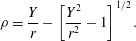 $$\begin{eqnarray}\unicode[STIX]{x1D70C}=\frac{Y}{r}-\left[\frac{Y^{2}}{r^{2}}-1\right]^{1/2}.\end{eqnarray}$$
With
 $\dot{\unicode[STIX]{x1D6FE}}=0$
and
$\dot{\unicode[STIX]{x1D6FE}}=0$
and
 $V_{1}=0$
, these equations were derived by Crowdy (Reference Crowdy2011) using complex variable methods; with
$V_{1}=0$
, these equations were derived by Crowdy (Reference Crowdy2011) using complex variable methods; with
 $\dot{\unicode[STIX]{x1D6FE}}=0$
, they were later generalized to the case
$\dot{\unicode[STIX]{x1D6FE}}=0$
, they were later generalized to the case
 $V_{1}\neq 0$
by Yazdi et al. (Reference Yazdi, Ardekani and Borham2014) using an approach based on bipolar coordinates. The new feature in (1.1) is the addition of the shear-dependent terms with
$V_{1}\neq 0$
by Yazdi et al. (Reference Yazdi, Ardekani and Borham2014) using an approach based on bipolar coordinates. The new feature in (1.1) is the addition of the shear-dependent terms with
 $\dot{\unicode[STIX]{x1D6FE}}\neq 0$
.
$\dot{\unicode[STIX]{x1D6FE}}\neq 0$
.
We also demonstrate, in § 5, the new result that the dynamical system (1.1) has an associated Hamiltonian structure both with and without a background shear flow. It is interesting to note that theoretical models of swimmers in Poiseuille flow derived by previous authors (Zöttl & Stark Reference Zöttl and Stark2012, Reference Zöttl and Stark2013) have also been shown to be Hamiltonian; those models do not, however, incorporate hydrodynamic interactions with the wall and assume that the swimmer is sufficiently far from the wall that those interactions can be neglected. An oscillatory swimmer motion in a cylindrical tube has been reported in a detailed numerical calculation incorporating swimmer–wall hydrodynamic interactions by Zhu, Lauga & Brandt (Reference Zhu, Lauga and Brandt2013). In contrast, the analytically expressed model (1.1) is valid for any separation of the swimmer from the wall and fully accounts for hydrodynamic interactions, without any approximations. In § 6, we use all of the aforementioned results to investigate how the periodic orbits of a swimmer actuated by a particular two-mode tangential slip profile are modulated by the background shear flow.
2 Problem setting
2.1 Flow configuration
We assume that a circular treadmiller of radius
 $r$
is situated at distance
$r$
is situated at distance
 $Y(t)$
above a plane no-slip wall (figure 1). Its centre is at
$Y(t)$
above a plane no-slip wall (figure 1). Its centre is at
 $\boldsymbol{x}_{\boldsymbol{d}}(t)=(X(t),Y(t))$
. The ambient fluid is assumed to have viscosity
$\boldsymbol{x}_{\boldsymbol{d}}(t)=(X(t),Y(t))$
. The ambient fluid is assumed to have viscosity
 $\unicode[STIX]{x1D707}$
. A background shear with shear rate
$\unicode[STIX]{x1D707}$
. A background shear with shear rate
 $\dot{\unicode[STIX]{x1D6FE}}$
is present, so that, as
$\dot{\unicode[STIX]{x1D6FE}}$
is present, so that, as
 $y\rightarrow \infty$
,
$y\rightarrow \infty$
,
 $$\begin{eqnarray}(u,v)\rightarrow (\dot{\unicode[STIX]{x1D6FE}}y,0).\end{eqnarray}$$
A tangential treadmilling velocity is present on the swimmer boundary, causing it to move in a force- and torque-free motion near the wall. This tangential slip can be chosen as we like, and we will consider an arbitrary smooth axisymmetric velocity profile, which is discussed in detail in § 4. The key difference between the flow configuration here and that considered earlier in Crowdy (Reference Crowdy2011) is the presence of the background shear.

Figure 1. Circular treadmiller, of radius
 $r$
and orientation
$r$
and orientation
 $\unicode[STIX]{x1D703}(t)$
, with centre
$\unicode[STIX]{x1D703}(t)$
, with centre
 $\boldsymbol{x}_{\boldsymbol{d}}(t)=(X(t),Y(t))$
above a no-slip wall along
$\boldsymbol{x}_{\boldsymbol{d}}(t)=(X(t),Y(t))$
above a no-slip wall along
 $y=0$
.
$y=0$
.
2.2 Reciprocal theorem
Let
 $D$
denote the domain shown in figure 2(b) and let
$D$
denote the domain shown in figure 2(b) and let
 $\unicode[STIX]{x2202}D$
denote its boundary, including the semicircle
$\unicode[STIX]{x2202}D$
denote its boundary, including the semicircle
 $C_{S}$
of radius
$C_{S}$
of radius
 $S$
around the point at infinity; later, we will take the limit
$S$
around the point at infinity; later, we will take the limit
 $S\rightarrow \infty$
. The reciprocal theorem based on this domain choice implies the following integral relation with respect to the velocity vectors and the stress tensors,
$S\rightarrow \infty$
. The reciprocal theorem based on this domain choice implies the following integral relation with respect to the velocity vectors and the stress tensors,
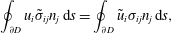 $$\begin{eqnarray}\oint _{\unicode[STIX]{x2202}D}u_{i}\tilde{\unicode[STIX]{x1D70E}}_{ij}n_{j}\,\text{d}s=\oint _{\unicode[STIX]{x2202}D}\tilde{u} _{i}\unicode[STIX]{x1D70E}_{ij}n_{j}\,\text{d}s,\end{eqnarray}$$
between two distinct solutions of the Stokes equations in the same domain, i.e.
 $$\begin{eqnarray}\frac{\unicode[STIX]{x2202}u_{i}}{\unicode[STIX]{x2202}x_{i}}=0,\quad \frac{\unicode[STIX]{x2202}\unicode[STIX]{x1D70E}_{ij}}{\unicode[STIX]{x2202}x_{j}}=0;\quad \frac{\unicode[STIX]{x2202}\tilde{u} _{i}}{\unicode[STIX]{x2202}x_{i}}=0,\quad \frac{\unicode[STIX]{x2202}\tilde{\unicode[STIX]{x1D70E}}_{ij}}{\unicode[STIX]{x2202}x_{j}}=0.\end{eqnarray}$$
These are solutions to two different boundary value problems. We make the following special choices:
 $(u_{i},\unicode[STIX]{x1D70E}_{ij})$
is the solution of the Jeffrey–Onishi boundary value problem just described (for a solid cylinder translating and rotating near a no-slip wall);
$(u_{i},\unicode[STIX]{x1D70E}_{ij})$
is the solution of the Jeffrey–Onishi boundary value problem just described (for a solid cylinder translating and rotating near a no-slip wall);
 $(\tilde{u} _{i},\tilde{\unicode[STIX]{x1D70E}}_{ij})$
is taken to be the flow associated with a force-free and torque-free treadmilling swimmer in a linear shear with shear rate
$(\tilde{u} _{i},\tilde{\unicode[STIX]{x1D70E}}_{ij})$
is taken to be the flow associated with a force-free and torque-free treadmilling swimmer in a linear shear with shear rate
 $\dot{\unicode[STIX]{x1D6FE}}$
.
$\dot{\unicode[STIX]{x1D6FE}}$
.

Figure 2. Contours of integration in (a) the
 $\unicode[STIX]{x1D701}$
plane and (b) the
$\unicode[STIX]{x1D701}$
plane and (b) the
 $z$
plane.
$z$
plane.
In both problems, the fluid velocity on the wall vanishes, so (2.2) becomes
 $$\begin{eqnarray}\displaystyle & \displaystyle -\oint _{|z-z_{d}|=r}u_{i}\tilde{\unicode[STIX]{x1D70E}}_{ij}n_{j}\,\text{d}s+\lim _{S\rightarrow \infty }\int _{C_{S}}u_{i}\tilde{\unicode[STIX]{x1D70E}}_{ij}n_{j}\,\text{d}s=-\oint _{|z-z_{d}|=r}\tilde{u} _{i}\unicode[STIX]{x1D70E}_{ij}n_{j}\,\text{d}s+\lim _{S\rightarrow \infty }\int _{C_{S}}\tilde{u} _{i}\unicode[STIX]{x1D70E}_{ij}n_{j}\,\text{d}s,\qquad & \displaystyle\end{eqnarray}$$
where
 $C_{S}$
is a semicircle of radius
$C_{S}$
is a semicircle of radius
 $S$
centred at
$S$
centred at
 $z=0$
. On the cylinder boundary,
$z=0$
. On the cylinder boundary,
 $$\begin{eqnarray}u_{i}=\boldsymbol{U}_{i}+\unicode[STIX]{x1D716}_{imn}\unicode[STIX]{x1D734}_{m}(x_{n}-x_{dn}),\end{eqnarray}$$
where
 $\boldsymbol{U}=({\mathcal{U}},{\mathcal{V}},0)$
and
$\boldsymbol{U}=({\mathcal{U}},{\mathcal{V}},0)$
and
 $\unicode[STIX]{x1D734}=(0,0,\unicode[STIX]{x1D6FA})$
, and where
$\unicode[STIX]{x1D734}=(0,0,\unicode[STIX]{x1D6FA})$
, and where
 ${\mathcal{U}}$
and
${\mathcal{U}}$
and
 ${\mathcal{V}}$
are the velocity components of the cylinder and
${\mathcal{V}}$
are the velocity components of the cylinder and
 $\unicode[STIX]{x1D6FA}$
is its angular velocity. We use
$\unicode[STIX]{x1D6FA}$
is its angular velocity. We use
 $x_{dn}$
to denote the components of
$x_{dn}$
to denote the components of
 $\boldsymbol{x}_{\boldsymbol{d}}$
. Similarly, we let
$\boldsymbol{x}_{\boldsymbol{d}}$
. Similarly, we let
 $\boldsymbol{U}^{\prime }=({\mathcal{U}}^{\prime },{\mathcal{V}}^{\prime },0)$
and
$\boldsymbol{U}^{\prime }=({\mathcal{U}}^{\prime },{\mathcal{V}}^{\prime },0)$
and
 $\unicode[STIX]{x1D734}^{\prime }=(0,0,\unicode[STIX]{x1D6FA}^{\prime })$
, where
$\unicode[STIX]{x1D734}^{\prime }=(0,0,\unicode[STIX]{x1D6FA}^{\prime })$
, where
 $\unicode[STIX]{x1D6FA}^{\prime }$
is the angular velocity of the swimmer, so that, on the swimmer boundary,
$\unicode[STIX]{x1D6FA}^{\prime }$
is the angular velocity of the swimmer, so that, on the swimmer boundary,
 $$\begin{eqnarray}\tilde{u} _{i}=\boldsymbol{U}_{i}^{\prime }+\unicode[STIX]{x1D716}_{imn}\unicode[STIX]{x1D734}_{m}^{\prime }(x_{n}-x_{dn})+\boldsymbol{U}_{si},\end{eqnarray}$$
where
 $\boldsymbol{U}_{si}$
denotes the imposed treadmilling action. We can therefore write
$\boldsymbol{U}_{si}$
denotes the imposed treadmilling action. We can therefore write
 $$\begin{eqnarray}\displaystyle & & \displaystyle -\oint _{|z-z_{d}|=r}(\boldsymbol{U}_{i}+\unicode[STIX]{x1D716}_{imn}\unicode[STIX]{x1D734}_{m}(x_{n}-x_{dn}))\tilde{\unicode[STIX]{x1D70E}}_{ij}n_{j}\,\text{d}s+\lim _{S\rightarrow \infty }\int _{C_{S}}u_{i}\tilde{\unicode[STIX]{x1D70E}}_{ij}n_{j}\,\text{d}s\nonumber\\ \displaystyle & & \displaystyle \quad =-\oint _{|z-z_{d}|=r}(\boldsymbol{U}_{i}^{\prime }+\unicode[STIX]{x1D716}_{imn}\unicode[STIX]{x1D734}_{m}^{\prime }(x_{n}-x_{dn})+\boldsymbol{U}_{si})\unicode[STIX]{x1D70E}_{ij}n_{j}\,\text{d}s+\lim _{S\rightarrow \infty }\int _{C_{S}}\tilde{u} _{i}\unicode[STIX]{x1D70E}_{ij}n_{j}\,\text{d}s.\quad\end{eqnarray}$$
The left-hand side can be written as
 $$\begin{eqnarray}\displaystyle & & \displaystyle -\boldsymbol{U}_{i}\oint _{|z-z_{d}|=r}\tilde{\unicode[STIX]{x1D70E}}_{ij}n_{j}\,\text{d}s-\unicode[STIX]{x1D734}_{m}\oint _{|z-z_{d}|=r}\unicode[STIX]{x1D716}_{mni}(x_{n}-x_{dn})\tilde{\unicode[STIX]{x1D70E}}_{ij}n_{j}\,\text{d}s\nonumber\\ \displaystyle & & \displaystyle \quad +\,\lim _{S\rightarrow \infty }\int _{C_{S}}u_{i}\tilde{\unicode[STIX]{x1D70E}}_{ij}n_{j}\,\text{d}s=-\boldsymbol{F}^{\prime }\boldsymbol{\cdot }\boldsymbol{U}-\unicode[STIX]{x1D734}\boldsymbol{\cdot }\boldsymbol{T}^{\prime }+\lim _{S\rightarrow \infty }\int _{C_{S}}u_{i}\tilde{\unicode[STIX]{x1D70E}}_{ij}n_{j}\,\text{d}s,\end{eqnarray}$$
where
 $\boldsymbol{F}^{\prime }$
and
$\boldsymbol{F}^{\prime }$
and
 $\boldsymbol{T}^{\prime }$
are the force and torque on the swimmer. However, these are both zero. It follows that
$\boldsymbol{T}^{\prime }$
are the force and torque on the swimmer. However, these are both zero. It follows that
 $$\begin{eqnarray}\displaystyle \lim _{S\rightarrow \infty }\int _{C_{S}}u_{i}\tilde{\unicode[STIX]{x1D70E}}_{ij}n_{j}\,\text{d}s & = & \displaystyle -\oint _{|z-z_{d}|=r}(\boldsymbol{U}_{i}^{\prime }+\unicode[STIX]{x1D716}_{imn}\unicode[STIX]{x1D734}_{m}^{\prime }(x_{n}-x_{dn})+\boldsymbol{U}_{si})\unicode[STIX]{x1D70E}_{ij}n_{j}\,\text{d}s\nonumber\\ \displaystyle & & \displaystyle +\,\lim _{S\rightarrow \infty }\int _{C_{S}}\tilde{u} _{i}\unicode[STIX]{x1D70E}_{ij}n_{j}\,\text{d}s.\end{eqnarray}$$
On rearrangement, and by similar arguments to those just used, we find
 $$\begin{eqnarray}\boldsymbol{F}\boldsymbol{\cdot }\boldsymbol{U}^{\prime }+\unicode[STIX]{x1D734}^{\prime }\boldsymbol{\cdot }\boldsymbol{T}=-\oint _{|z-z_{d}|=r}\boldsymbol{U}_{si}\unicode[STIX]{x1D70E}_{ij}n_{j}\,\text{d}s+\underbrace{\lim _{S\rightarrow \infty }\int _{C_{S}}(\tilde{u} _{i}\unicode[STIX]{x1D70E}_{ij}n_{j}-u_{i}\tilde{\unicode[STIX]{x1D70E}}_{ij}n_{j})\,\text{d}s}_{\text{shear}\text{-}\text{induced term}},\end{eqnarray}$$
where
 $\boldsymbol{F}$
and
$\boldsymbol{F}$
and
 $\boldsymbol{T}$
are the force and torque on the cylinder in the Jeffrey–Onishi problem.
$\boldsymbol{T}$
are the force and torque on the cylinder in the Jeffrey–Onishi problem.
The key difference between (2.10) and an analogous equation derived in Crowdy (Reference Crowdy2011) is the retention of the contribution from the integral around
 $C_{S}$
in the limit
$C_{S}$
in the limit
 $S\rightarrow \infty$
. In the absence of background shear, this term vanishes and (2.10) reduces to the equation considered in Crowdy (Reference Crowdy2011).
$S\rightarrow \infty$
. In the absence of background shear, this term vanishes and (2.10) reduces to the equation considered in Crowdy (Reference Crowdy2011).
2.3 Conformal mapping
Following Crowdy (Reference Crowdy2011), we now compute these additional integral contributions using a complex variable formulation together with the convenient complex variable form of the Jeffrey–Onishi solution derived using conformal mapping ideas. The general solution for the streamfunction associated with a two-dimensional Stokes flow can be written as
 $$\begin{eqnarray}\unicode[STIX]{x1D713}(z,\overline{z})=\text{Im}[\overline{z}f(z)+g(z)],\end{eqnarray}$$
where
 $f(z)$
and
$f(z)$
and
 $g(z)$
are two functions that are analytic in the fluid region (and are often called Goursat functions). We will use
$g(z)$
are two functions that are analytic in the fluid region (and are often called Goursat functions). We will use
 $f(z)$
and
$f(z)$
and
 $g(z)$
to denote the Goursat functions for the dragging problem and
$g(z)$
to denote the Goursat functions for the dragging problem and
 $\tilde{f}(z)$
and
$\tilde{f}(z)$
and
 $\tilde{g}(z)$
to denote the Goursat functions for the swimmer in shear. These functions will be time-dependent, but, due to the quasisteady nature of the flow generated by the swimmer, it is natural to suppress this explicit dependence on time in our notation.
$\tilde{g}(z)$
to denote the Goursat functions for the swimmer in shear. These functions will be time-dependent, but, due to the quasisteady nature of the flow generated by the swimmer, it is natural to suppress this explicit dependence on time in our notation.
We introduce the conformal mapping
 $$\begin{eqnarray}z=X+\text{i}R\left[\frac{\unicode[STIX]{x1D701}+1}{\unicode[STIX]{x1D701}-1}\right]\end{eqnarray}$$
from the annulus
 $\unicode[STIX]{x1D70C}<|\unicode[STIX]{x1D701}|<1$
to the fluid region exterior to the treadmilling swimmer. We let the centre of the swimmer have complex position
$\unicode[STIX]{x1D70C}<|\unicode[STIX]{x1D701}|<1$
to the fluid region exterior to the treadmilling swimmer. We let the centre of the swimmer have complex position
 $z_{d}=X+\text{i}Y$
. It is known (Crowdy Reference Crowdy2011) that
$z_{d}=X+\text{i}Y$
. It is known (Crowdy Reference Crowdy2011) that
 $$\begin{eqnarray}\unicode[STIX]{x1D70C}=\frac{Y}{r}-\left[\frac{Y^{2}}{r^{2}}-1\right]^{1/2},\quad \frac{1}{\unicode[STIX]{x1D70C}}=\frac{Y}{r}+\left[\frac{Y^{2}}{r^{2}}-1\right]^{1/2},\quad \frac{z-z_{d}}{r}=-\frac{\text{i}}{\unicode[STIX]{x1D70C}}\left[\frac{\unicode[STIX]{x1D701}-\unicode[STIX]{x1D70C}^{2}}{\unicode[STIX]{x1D701}-1}\right]\!.~\end{eqnarray}$$
As the swimmer evolves, the parameters
 $X$
and
$X$
and
 $Y$
, and hence
$Y$
, and hence
 $R,\unicode[STIX]{x1D70C}$
and
$R,\unicode[STIX]{x1D70C}$
and
 $z_{d}$
, will be time-evolving parameters, but, again, we suppress this dependence in our notation. When the swimmer is far from the wall, so that
$z_{d}$
, will be time-evolving parameters, but, again, we suppress this dependence in our notation. When the swimmer is far from the wall, so that
 $Y/r\rightarrow \infty$
, then
$Y/r\rightarrow \infty$
, then
 $\unicode[STIX]{x1D70C}\rightarrow 0$
; the situation where the swimmer draws close to the wall, so that
$\unicode[STIX]{x1D70C}\rightarrow 0$
; the situation where the swimmer draws close to the wall, so that
 $Y/r\rightarrow 1$
, corresponds to
$Y/r\rightarrow 1$
, corresponds to
 $\unicode[STIX]{x1D70C}\rightarrow 1$
.
$\unicode[STIX]{x1D70C}\rightarrow 1$
.
For large
 $S$
, the preimage of the large semicircular contour
$S$
, the preimage of the large semicircular contour
 $C_{S}$
will be a small semicircular contour
$C_{S}$
will be a small semicircular contour
 $C_{\unicode[STIX]{x1D716}}$
of radius
$C_{\unicode[STIX]{x1D716}}$
of radius
 $\unicode[STIX]{x1D716}\ll 1$
centred at
$\unicode[STIX]{x1D716}\ll 1$
centred at
 $\unicode[STIX]{x1D701}=1$
; see figure 2. In complex variable notation,
$\unicode[STIX]{x1D701}=1$
; see figure 2. In complex variable notation,
 $$\begin{eqnarray}\unicode[STIX]{x1D70E}_{ij}n_{j}\mapsto 2\unicode[STIX]{x1D707}\text{i}\frac{\text{d}H}{\text{d}s},\quad \tilde{\unicode[STIX]{x1D70E}}_{ij}n_{j}\mapsto 2\unicode[STIX]{x1D707}\text{i}\frac{\text{d}\tilde{H}}{\text{d}s},\end{eqnarray}$$
where
 $$\begin{eqnarray}H\equiv f(z)+z\overline{f^{\prime }(z)}+\overline{g^{\prime }(z)},\quad \tilde{H}\equiv \tilde{f}(z)+z\overline{\tilde{f}^{\prime }(z)}+\overline{\tilde{g}^{\prime }(z)},\end{eqnarray}$$
and where we use the notation
 $\mapsto$
to denote the complex variable form of a two-dimensional vector quantity:
$\mapsto$
to denote the complex variable form of a two-dimensional vector quantity:
 $\boldsymbol{a}=(a_{x},a_{y})\mapsto a_{x}+\text{i}a_{y}$
. It follows that the complex variable form of the new integral contribution in (2.10) is
$\boldsymbol{a}=(a_{x},a_{y})\mapsto a_{x}+\text{i}a_{y}$
. It follows that the complex variable form of the new integral contribution in (2.10) is
 $$\begin{eqnarray}\lim _{S\rightarrow \infty }\int _{C_{S}}(\tilde{u} _{i}\unicode[STIX]{x1D70E}_{ij}n_{j}-u_{i}\tilde{\unicode[STIX]{x1D70E}}_{ij}n_{j})\,\text{d}s=\lim _{\unicode[STIX]{x1D716}\rightarrow 0}\text{Re}\left[2\unicode[STIX]{x1D707}\text{i}\left\{\int _{C_{\unicode[STIX]{x1D716}}}(\tilde{u} -\text{i}\tilde{v})\,\text{d}H-(u-\text{i}v)\text{d}\tilde{H}\right\}\right].\end{eqnarray}$$
3 Shear effects
We now show how to compute the additional shear-induced term on the right-hand side of (2.16). Since it involves a contribution from around the large circular contour
 $C_{S}$
, where
$C_{S}$
, where
 $S\rightarrow \infty$
, in the physical plane, this implies evaluation of an integral around a small contour
$S\rightarrow \infty$
, in the physical plane, this implies evaluation of an integral around a small contour
 $C_{\unicode[STIX]{x1D716}}$
of radius
$C_{\unicode[STIX]{x1D716}}$
of radius
 $\unicode[STIX]{x1D716}\rightarrow 0$
around
$\unicode[STIX]{x1D716}\rightarrow 0$
around
 $\unicode[STIX]{x1D701}=1$
in the parametric
$\unicode[STIX]{x1D701}=1$
in the parametric
 $\unicode[STIX]{x1D701}$
plane, as indicated schematically in figure 2.
$\unicode[STIX]{x1D701}$
plane, as indicated schematically in figure 2.
For the swimmer problem, we have
 $$\begin{eqnarray}\tilde{f}(z)\sim \frac{\text{i}\dot{\unicode[STIX]{x1D6FE}}z}{4}+O(1/z),\quad \tilde{g}^{\prime }(z)\sim -\frac{\text{i}\dot{\unicode[STIX]{x1D6FE}}z}{2}+O(1/z^{2}),\end{eqnarray}$$
in order that
 $\tilde{u} -\text{i}\tilde{v}\rightarrow \dot{\unicode[STIX]{x1D6FE}}y+O(1/|z|)$
. Written in terms of
$\tilde{u} -\text{i}\tilde{v}\rightarrow \dot{\unicode[STIX]{x1D6FE}}y+O(1/|z|)$
. Written in terms of
 $\unicode[STIX]{x1D701}$
and
$\unicode[STIX]{x1D701}$
and
 $\overline{\unicode[STIX]{x1D701}}$
, this is
$\overline{\unicode[STIX]{x1D701}}$
, this is
 $$\begin{eqnarray}\tilde{u} -\text{i}\tilde{v}\rightarrow \dot{\unicode[STIX]{x1D6FE}}R\frac{(\unicode[STIX]{x1D701}\overline{\unicode[STIX]{x1D701}}-1)}{(\unicode[STIX]{x1D701}-1)(\overline{\unicode[STIX]{x1D701}}-1)}+O(|\unicode[STIX]{x1D701}-1|).\end{eqnarray}$$
It can be verified that, as
 $|z|\rightarrow \infty$
, or as
$|z|\rightarrow \infty$
, or as
 $\unicode[STIX]{x1D701}\rightarrow 1$
,
$\unicode[STIX]{x1D701}\rightarrow 1$
,
 $$\begin{eqnarray}\tilde{H}=\tilde{f}(z)+z\overline{\tilde{f}^{\prime }(z)}+\overline{\tilde{g}^{\prime }(z)}\sim \frac{\text{i}\dot{\unicode[STIX]{x1D6FE}}\overline{z}}{2}+O(1/|z|).\end{eqnarray}$$
Written in terms of
 $\unicode[STIX]{x1D701}$
and
$\unicode[STIX]{x1D701}$
and
 $\overline{\unicode[STIX]{x1D701}}$
, this is
$\overline{\unicode[STIX]{x1D701}}$
, this is
 $$\begin{eqnarray}\tilde{H}=\frac{\dot{\unicode[STIX]{x1D6FE}}R}{2}\left(\frac{\overline{\unicode[STIX]{x1D701}}+1}{\overline{\unicode[STIX]{x1D701}}-1}\right)+O(|\unicode[STIX]{x1D701}-1|).\end{eqnarray}$$
On substitution of the following parametrizations of the contour
 $C_{\unicode[STIX]{x1D716}}$
,
$C_{\unicode[STIX]{x1D716}}$
,
 $$\begin{eqnarray}\unicode[STIX]{x1D701}=1+\unicode[STIX]{x1D716}\text{e}^{\text{i}\unicode[STIX]{x1D703}},\quad \overline{\unicode[STIX]{x1D701}}=1+\unicode[STIX]{x1D716}\text{e}^{-\text{i}\unicode[STIX]{x1D703}},\end{eqnarray}$$
we find
 $$\begin{eqnarray}\tilde{u} -\text{i}\tilde{v}=\frac{\dot{\unicode[STIX]{x1D6FE}}R}{\unicode[STIX]{x1D716}}[\text{e}^{\text{i}\unicode[STIX]{x1D703}}+\text{e}^{-\text{i}\unicode[STIX]{x1D703}}]+o(1/\unicode[STIX]{x1D716}),\quad \tilde{H}=\frac{\dot{\unicode[STIX]{x1D6FE}}R\text{e}^{\text{i}\unicode[STIX]{x1D703}}}{\unicode[STIX]{x1D716}}+o(1/\unicode[STIX]{x1D716}).\end{eqnarray}$$
On the other hand, for the dragging problem, it can be shown from the results in Crowdy (Reference Crowdy2011) that
 $$\begin{eqnarray}H=F(\unicode[STIX]{x1D701})+F(1/\overline{\unicode[STIX]{x1D701}})+\frac{\overline{F}^{\prime }(\overline{\unicode[STIX]{x1D701}})}{\overline{z}^{\prime }(\overline{\unicode[STIX]{x1D701}})}[z(\unicode[STIX]{x1D701})-z(1/\overline{\unicode[STIX]{x1D701}})],\end{eqnarray}$$
implying the expression
 $$\begin{eqnarray}H=F_{d}\log \left[\frac{\unicode[STIX]{x1D701}}{\overline{\unicode[STIX]{x1D701}}}\right]+B\left[\overline{\unicode[STIX]{x1D701}}+\frac{1}{\unicode[STIX]{x1D701}}\right]+C\left[\unicode[STIX]{x1D701}+\frac{1}{\overline{\unicode[STIX]{x1D701}}}\right]+\left[\frac{\overline{F_{d}}}{\overline{\unicode[STIX]{x1D701}}}-\frac{\overline{B}}{\overline{\unicode[STIX]{x1D701}}^{2}}+\overline{C}\right](\unicode[STIX]{x1D701}\overline{\unicode[STIX]{x1D701}}-1)\frac{\overline{\unicode[STIX]{x1D701}}-1}{\unicode[STIX]{x1D701}-1}.\end{eqnarray}$$
Moreover,
 $$\begin{eqnarray}u-\text{i}v=-F(\unicode[STIX]{x1D701})+F(1/\overline{\unicode[STIX]{x1D701}})+\frac{\overline{F}^{\prime }(\overline{\unicode[STIX]{x1D701}})}{\overline{z}^{\prime }(\overline{\unicode[STIX]{x1D701}})}[z(\unicode[STIX]{x1D701})-z(1/\overline{\unicode[STIX]{x1D701}})],\end{eqnarray}$$
implying the expression
 $$\begin{eqnarray}u-\text{i}v=-\overline{F_{d}}\log |\unicode[STIX]{x1D701}|^{2}+\overline{B}\left[\unicode[STIX]{x1D701}-\frac{1}{\overline{\unicode[STIX]{x1D701}}}\right]+\overline{C}\left[\frac{1}{\unicode[STIX]{x1D701}}-\overline{\unicode[STIX]{x1D701}}\right]+\left[\frac{F_{d}}{\unicode[STIX]{x1D701}}-\frac{B}{\unicode[STIX]{x1D701}^{2}}+C\right](\unicode[STIX]{x1D701}\overline{\unicode[STIX]{x1D701}}-1)\frac{\unicode[STIX]{x1D701}-1}{\overline{\unicode[STIX]{x1D701}}-1}.\end{eqnarray}$$
On substitution of the parametrizations (3.5), we find
 $$\begin{eqnarray}\left.\begin{array}{@{}c@{}}H\sim 2(B+C)+\unicode[STIX]{x1D716}[(F_{d}-B+C)(\text{e}^{\text{i}\unicode[STIX]{x1D703}}-\text{e}^{-\text{i}\unicode[STIX]{x1D703}})+(\overline{F_{d}}-\overline{B}+\overline{C})(\text{e}^{-\text{i}\unicode[STIX]{x1D703}}+\text{e}^{-3\text{i}\unicode[STIX]{x1D703}})]+O(\unicode[STIX]{x1D716}^{2}),\\ u-\text{i}v\sim \unicode[STIX]{x1D716}[(F_{d}-B+C)(\text{e}^{\text{i}\unicode[STIX]{x1D703}}+\text{e}^{3\text{i}\unicode[STIX]{x1D703}})-(\overline{F_{d}}-\overline{B}+\overline{C})(\text{e}^{\text{i}\unicode[STIX]{x1D703}}+\text{e}^{-\text{i}\unicode[STIX]{x1D703}})]+O(\unicode[STIX]{x1D716}^{2}).\end{array}\right\}\end{eqnarray}$$
On combining all of these results, we find
 $$\begin{eqnarray}\displaystyle & & \displaystyle \int _{C_{\unicode[STIX]{x1D716}}}(u^{\prime }-\text{i}v^{\prime })\,\text{d}H-(u-\text{i}v)\,\text{d}\tilde{H}\nonumber\\ \displaystyle & & \displaystyle \quad =-\text{i}\dot{\unicode[STIX]{x1D6FE}}R\left\{\int _{\unicode[STIX]{x03C0}/2}^{3\unicode[STIX]{x03C0}/2}(F_{d}-B+C)[(\text{e}^{\text{i}\unicode[STIX]{x1D703}}+\text{e}^{-\text{i}\unicode[STIX]{x1D703}})^{2}-(\text{e}^{2\text{i}\unicode[STIX]{x1D703}}+\text{e}^{4\text{i}\unicode[STIX]{x1D703}})]\,\text{d}\unicode[STIX]{x1D703}\right.\nonumber\\ \displaystyle & & \displaystyle \qquad +\left.(\overline{F_{d}}-\overline{B}+\overline{C})[\text{e}^{2\text{i}\unicode[STIX]{x1D703}}+1-(\text{e}^{\text{i}\unicode[STIX]{x1D703}}+\text{e}^{-\text{i}\unicode[STIX]{x1D703}})(\text{e}^{-\text{i}\unicode[STIX]{x1D703}}+3\text{e}^{-\text{i}\unicode[STIX]{x1D703}})]\,\text{d}\unicode[STIX]{x1D703}\vphantom{\int _{\unicode[STIX]{x03C0}/2}^{3\unicode[STIX]{x03C0}/2}}\right\}+o(1)\nonumber\\ \displaystyle & & \displaystyle \quad =-2\unicode[STIX]{x03C0}\text{i}\dot{\unicode[STIX]{x1D6FE}}R(F_{d}-B+C)+O(\unicode[STIX]{x1D716}).\end{eqnarray}$$
From (2.16) and (2.10), in the limit
 $\unicode[STIX]{x1D716}\rightarrow 0$
,
$\unicode[STIX]{x1D716}\rightarrow 0$
,
 $$\begin{eqnarray}\boldsymbol{F}\boldsymbol{\cdot }\boldsymbol{U}^{\prime }+\unicode[STIX]{x1D734}^{\prime }\boldsymbol{\cdot }\boldsymbol{T}=-\oint _{|z-z_{d}|=r}\boldsymbol{U}_{si}\unicode[STIX]{x1D70E}_{ij}n_{j}\,\text{d}s+\underbrace{4\unicode[STIX]{x03C0}\unicode[STIX]{x1D707}R\dot{\unicode[STIX]{x1D6FE}}\text{Re}[F_{d}-\unicode[STIX]{x1D70C}^{2}\overline{C}+C]}_{\text{shear}\text{-}\text{induced term}},\end{eqnarray}$$
where we have used the fact, derived in Crowdy (Reference Crowdy2011), that
 $B=\unicode[STIX]{x1D70C}^{2}\overline{C}$
.
$B=\unicode[STIX]{x1D70C}^{2}\overline{C}$
.
3.1 Three comparison flows
Following Crowdy (Reference Crowdy2011), to derive the equations of motion, we make three independent choices of solution to the dragging problem. Due to the linearity of the flow problem, it is convenient to decompose the components of the speed of the swimmer as follows:
 $$\begin{eqnarray}{\mathcal{U}}^{\prime }={\mathcal{U}}_{tread}^{\prime }+{\mathcal{U}}_{shear}^{\prime },\quad {\mathcal{V}}^{\prime }={\mathcal{V}}_{tread}^{\prime }+{\mathcal{V}}_{shear}^{\prime },\quad \unicode[STIX]{x1D6FA}^{\prime }=\unicode[STIX]{x1D6FA}_{tread}^{\prime }+\unicode[STIX]{x1D6FA}_{shear}^{\prime },\end{eqnarray}$$
where it has already been demonstrated in Crowdy (Reference Crowdy2011, Reference Crowdy2013) how to compute the speeds
 ${\mathcal{U}}_{tread}^{\prime },{\mathcal{V}}_{tread}^{\prime }$
and
${\mathcal{U}}_{tread}^{\prime },{\mathcal{V}}_{tread}^{\prime }$
and
 $\unicode[STIX]{x1D6FA}_{tread}^{\prime }$
induced by the treadmilling action. Here, we focus on calculating the additional terms
$\unicode[STIX]{x1D6FA}_{tread}^{\prime }$
induced by the treadmilling action. Here, we focus on calculating the additional terms
 ${\mathcal{U}}_{shear}^{\prime },{\mathcal{V}}_{shear}^{\prime }$
and
${\mathcal{U}}_{shear}^{\prime },{\mathcal{V}}_{shear}^{\prime }$
and
 $\unicode[STIX]{x1D6FA}_{shear}^{\prime }$
due to the background shear.
$\unicode[STIX]{x1D6FA}_{shear}^{\prime }$
due to the background shear.
3.1.1 Angular velocity
 $\unicode[STIX]{x1D6FA}_{shear}^{\prime }$

First, let
 $U=0$
,
$U=0$
,
 $\unicode[STIX]{x1D6FA}=1$
. Then, it follows (Crowdy Reference Crowdy2011) that
$\unicode[STIX]{x1D6FA}=1$
. Then, it follows (Crowdy Reference Crowdy2011) that
 $$\begin{eqnarray}F_{d}=0,\quad C=\frac{2R\unicode[STIX]{x1D70C}^{2}}{(1-\unicode[STIX]{x1D70C}^{2})^{3}},\quad T=-4\unicode[STIX]{x03C0}\unicode[STIX]{x1D707}r^{2}\left(\frac{1+\unicode[STIX]{x1D70C}^{2}}{1-\unicode[STIX]{x1D70C}^{2}}\right).\end{eqnarray}$$
It follows from (3.13) that
 $$\begin{eqnarray}T\unicode[STIX]{x1D6FA}_{shear}^{\prime }=4\unicode[STIX]{x03C0}\unicode[STIX]{x1D707}\dot{\unicode[STIX]{x1D6FE}}R\frac{2R\unicode[STIX]{x1D70C}^{2}}{(1-\unicode[STIX]{x1D70C}^{2})^{2}},\end{eqnarray}$$
implying
 $$\begin{eqnarray}\unicode[STIX]{x1D6FA}_{shear}^{\prime }=-\frac{\dot{\unicode[STIX]{x1D6FE}}}{2}\left[\frac{1-\unicode[STIX]{x1D70C}^{2}}{1+\unicode[STIX]{x1D70C}^{2}}\right],\end{eqnarray}$$
where we have used the fact (Crowdy Reference Crowdy2011) that
 $$\begin{eqnarray}\frac{R}{r}=\frac{\unicode[STIX]{x1D70C}^{2}-1}{2\unicode[STIX]{x1D70C}}.\end{eqnarray}$$
3.1.2 Velocity
${\mathcal{U}}_{shear}^{\prime }$
parallel to wall

Next, let
 $\unicode[STIX]{x1D6FA}=0$
and
$\unicode[STIX]{x1D6FA}=0$
and
 $U=1$
. It follows that (Crowdy Reference Crowdy2011)
$U=1$
. It follows that (Crowdy Reference Crowdy2011)
 $$\begin{eqnarray}F_{d}=-\frac{1}{\log \unicode[STIX]{x1D70C}^{2}},\quad C=\frac{F_{d}}{(1-\unicode[STIX]{x1D70C}^{2})}=-\frac{1}{(1-\unicode[STIX]{x1D70C}^{2})\log \unicode[STIX]{x1D70C}^{2}},\quad F_{x}+\text{i}F_{y}=\frac{4\unicode[STIX]{x03C0}\unicode[STIX]{x1D707}}{\log \unicode[STIX]{x1D70C}}.\end{eqnarray}$$
Hence, (3.13) implies
 $$\begin{eqnarray}F_{x}{\mathcal{U}}_{shear}^{\prime }=-\frac{4\unicode[STIX]{x03C0}\dot{\unicode[STIX]{x1D6FE}}\unicode[STIX]{x1D707}R}{\log \unicode[STIX]{x1D70C}},\end{eqnarray}$$
from which we find
 $$\begin{eqnarray}{\mathcal{U}}_{shear}^{\prime }=\frac{\dot{\unicode[STIX]{x1D6FE}}r(1-\unicode[STIX]{x1D70C}^{2})}{2\unicode[STIX]{x1D70C}}.\end{eqnarray}$$
3.1.3 Velocity
${\mathcal{V}}_{shear}^{\prime }$
perpendicular to wall

Finally, let
 $\unicode[STIX]{x1D6FA}=0$
and
$\unicode[STIX]{x1D6FA}=0$
and
 $U=\text{i}$
. It follows that (Crowdy Reference Crowdy2011)
$U=\text{i}$
. It follows that (Crowdy Reference Crowdy2011)
 $$\begin{eqnarray}F_{d}=-\frac{\text{i}}{2(1-\unicode[STIX]{x1D70C}^{2})/(1+\unicode[STIX]{x1D70C}^{2})+\log \unicode[STIX]{x1D70C}^{2}},\quad C=-\frac{F_{d}}{1+\unicode[STIX]{x1D70C}^{2}}\end{eqnarray}$$
and
 $$\begin{eqnarray}F_{x}+\text{i}F_{y}=-\frac{4\unicode[STIX]{x03C0}\unicode[STIX]{x1D707}\text{i}}{\log (1/\unicode[STIX]{x1D70C})-(1-\unicode[STIX]{x1D70C}^{2})/(1+\unicode[STIX]{x1D70C}^{2})},\end{eqnarray}$$
which, from (3.13), implies that
 $$\begin{eqnarray}{\mathcal{V}}_{shear}^{\prime }=0.\end{eqnarray}$$
Hence, the background shear does not induce any swimmer motion perpendicular to the wall.
3.2 Summary
We can rewrite the final results in physical variables. On use of (2.13), the results we have found are
 $$\begin{eqnarray}{\mathcal{U}}_{shear}^{\prime }=\dot{\unicode[STIX]{x1D6FE}}[Y^{2}-r^{2}]^{1/2},\quad {\mathcal{V}}_{shear}^{\prime }=0,\quad \unicode[STIX]{x1D6FA}_{shear}^{\prime }=-\frac{\dot{\unicode[STIX]{x1D6FE}}}{2Y}[Y^{2}-r^{2}]^{1/2}.\end{eqnarray}$$
These contributions can be added to the contribution to the swimmer motion from the treadmilling action to produce the generalized dynamical systems for swimmers in shear. As a check on the results, it should be noted that in the limit
 $Y/r\rightarrow \infty$
, we find
$Y/r\rightarrow \infty$
, we find
 $$\begin{eqnarray}{\mathcal{U}}_{shear}^{\prime }=\dot{\unicode[STIX]{x1D6FE}}Y,\quad {\mathcal{V}}_{shear}^{\prime }=0,\quad \unicode[STIX]{x1D6FA}_{shear}^{\prime }=-\frac{\dot{\unicode[STIX]{x1D6FE}}}{2},\end{eqnarray}$$
which retrieves the known result for the motion of a solid cylinder in force- and torque-free motion in simple shear (see Crowdy (Reference Crowdy2016), for example).
The evolution equations (3.25) for a solid force-free and torque-free two-dimensional circular cylinder in a shear flow near a no-slip wall have been previously calculated in a thesis by Raasch using a separable solution method based on bipolar coordinates; a little-known paper, in German, summarizing that derivation appeared in 1961 (Raasch Reference Raasch1961). In principle, we could have simply invoked those results, but the derivation above using the reciprocal theorem and conformal mapping (rather than bipolar coordinates) is novel and is worth reporting in its own right. It is also a natural extension of previous work for swimming near a wall in the absence of shear (Crowdy Reference Crowdy2011, Reference Crowdy2013).
4 Swimmer dynamics
Consider a general axisymmetric treadmilling swimmer with a tangential velocity slip profile
 $V_{slip}$
such that the slip velocity
$V_{slip}$
such that the slip velocity
 $\boldsymbol{U}_{\boldsymbol{s}}$
on its boundary is given by
$\boldsymbol{U}_{\boldsymbol{s}}$
on its boundary is given by
 $$\begin{eqnarray}\boldsymbol{U}_{s}=V_{slip}\boldsymbol{t},\quad V_{slip}=\mathop{\sum }_{n=1}^{\infty }V_{n}\sin (n(\unicode[STIX]{x1D719}-\unicode[STIX]{x1D703})),\end{eqnarray}$$
where
 $\boldsymbol{t}$
denotes the unit tangent to the swimmer boundary and
$\boldsymbol{t}$
denotes the unit tangent to the swimmer boundary and
 $\unicode[STIX]{x1D719}$
is the angular coordinate on the surface relative to the centre of the swimmer. This is an extension of the treadmilling swimmer of Crowdy (Reference Crowdy2011) where only the
$\unicode[STIX]{x1D719}$
is the angular coordinate on the surface relative to the centre of the swimmer. This is an extension of the treadmilling swimmer of Crowdy (Reference Crowdy2011) where only the
 $n=2$
mode is considered in detail (such a swimmer does not move in the absence of wall effects). We can invoke the reciprocal theorem (2.10), without the shear-induced term,
$n=2$
mode is considered in detail (such a swimmer does not move in the absence of wall effects). We can invoke the reciprocal theorem (2.10), without the shear-induced term,
 $$\begin{eqnarray}\boldsymbol{F}\boldsymbol{\cdot }\boldsymbol{U}^{\prime }+\unicode[STIX]{x1D734}^{\prime }\boldsymbol{\cdot }\boldsymbol{T}=-\oint _{|z-z_{d}|=r}\boldsymbol{U}_{si}\unicode[STIX]{x1D70E}_{ij}n_{j}\,\text{d}s=-\text{Re}\left[2\unicode[STIX]{x1D707}\text{i}\oint _{|\unicode[STIX]{x1D701}|=\unicode[STIX]{x1D70C}}\overline{U}_{s}\frac{\text{d}H}{\text{d}\unicode[STIX]{x1D701}}\,\text{d}\unicode[STIX]{x1D701}\right],\end{eqnarray}$$
to derive the formulae for the linear and angular velocities due to the surface slip. In the second equality, we have used the complex variable form of the expression and rewritten the surface velocity as
 $$\begin{eqnarray}\boldsymbol{U}_{s}\mapsto U_{s}=V_{slip}\frac{\text{d}z}{\text{d}s},\end{eqnarray}$$
where we have used the fact that
 $\boldsymbol{t}\mapsto \text{d}z/\text{d}s$
. On use of (2.13), the surface velocity profile
$\boldsymbol{t}\mapsto \text{d}z/\text{d}s$
. On use of (2.13), the surface velocity profile
 $V_{slip}$
can be expressed in terms of
$V_{slip}$
can be expressed in terms of
 $\unicode[STIX]{x1D70C}$
and
$\unicode[STIX]{x1D70C}$
and
 $\unicode[STIX]{x1D701}$
in the form
$\unicode[STIX]{x1D701}$
in the form
 $$\begin{eqnarray}\displaystyle V_{slip}=\mathop{\sum }_{n=1}^{\infty }-\frac{\text{i}}{2}V_{n}\left[\left(-\frac{\text{i}}{\unicode[STIX]{x1D70C}}\left(\frac{\unicode[STIX]{x1D701}-\unicode[STIX]{x1D70C}^{2}}{\unicode[STIX]{x1D701}-1}\right)\right)^{n}\text{e}^{-\text{i}n\unicode[STIX]{x1D703}}-\left(-\frac{\text{i}}{\unicode[STIX]{x1D70C}}\left(\frac{\unicode[STIX]{x1D701}-\unicode[STIX]{x1D70C}^{2}}{\unicode[STIX]{x1D701}-1}\right)\right)^{-n}\text{e}^{\text{i}n\unicode[STIX]{x1D703}}\right]. & & \displaystyle\end{eqnarray}$$
We can therefore write
 $\overline{U_{s}}=\sum _{n=1}^{\infty }\overline{u_{s}}^{(n)}$
, where
$\overline{U_{s}}=\sum _{n=1}^{\infty }\overline{u_{s}}^{(n)}$
, where
 $$\begin{eqnarray}\overline{u}_{s}^{(n)}=\frac{\text{i}}{2}\left[c_{n}\text{i}^{n}\unicode[STIX]{x1D70C}^{n}\left(\frac{\unicode[STIX]{x1D701}-1}{\unicode[STIX]{x1D701}-\unicode[STIX]{x1D70C}^{2}}\right)^{n}-\overline{c_{n}}\text{i}^{-n}\unicode[STIX]{x1D70C}^{-n}\left(\frac{\unicode[STIX]{x1D701}-\unicode[STIX]{x1D70C}^{2}}{\unicode[STIX]{x1D701}-1}\right)^{n}\right]\overline{\frac{\text{d}z}{\text{d}s}},\end{eqnarray}$$
and where the notation
 $c_{n}=V_{n}\text{e}^{\text{i}n\unicode[STIX]{x1D703}}$
is introduced.
$c_{n}=V_{n}\text{e}^{\text{i}n\unicode[STIX]{x1D703}}$
is introduced.
One of the authors (Crowdy Reference Crowdy2013) has previously shown that for a general tangential slip profile of the form
 $$\begin{eqnarray}V_{slip}=b_{0}+\mathop{\sum }_{k=1}^{\infty }\left(b_{k}\unicode[STIX]{x1D701}^{k}+\overline{b_{k}}\frac{\unicode[STIX]{x1D70C}^{2k}}{\unicode[STIX]{x1D701}^{k}}\right),\end{eqnarray}$$
the associated velocities of a force-free and torque-free circular swimmer are
 $$\begin{eqnarray}({\mathcal{U}}_{tread}^{\prime },{\mathcal{V}}_{tread}^{\prime },\unicode[STIX]{x1D6FA}_{tread}^{\prime })=\left(\unicode[STIX]{x1D70C}\text{Re}[b_{1}],-\frac{\unicode[STIX]{x1D70C}(1-\unicode[STIX]{x1D70C}^{2})}{1+\unicode[STIX]{x1D70C}^{2}}\text{Im}[b_{1}],-\frac{1}{r}b_{0}-\frac{2\unicode[STIX]{x1D70C}^{2}}{r(1+\unicode[STIX]{x1D70C}^{2})}\text{Re}[b_{1}]\right).\end{eqnarray}$$
In other words, only the two coefficients
 $b_{0}$
and
$b_{0}$
and
 $b_{1}$
contribute to any net motion of the swimmer. If we denote by
$b_{1}$
contribute to any net motion of the swimmer. If we denote by
 $b_{0}^{(n)}$
and
$b_{0}^{(n)}$
and
 $b_{1}^{(n)}$
these relevant coefficients arising from the contribution
$b_{1}^{(n)}$
these relevant coefficients arising from the contribution
 $u_{s}^{(n)}$
, then some direct calculations lead to
$u_{s}^{(n)}$
, then some direct calculations lead to
 $$\begin{eqnarray}\left.\begin{array}{@{}c@{}}\displaystyle b_{0}^{(n)}=\frac{1}{2\unicode[STIX]{x03C0}\text{i}}\oint _{|\unicode[STIX]{x1D701}|=\unicode[STIX]{x1D70C}}\frac{|u_{s}^{(n)}|}{\unicode[STIX]{x1D701}}\,\text{d}\unicode[STIX]{x1D701}=\frac{\text{i}\unicode[STIX]{x1D70C}^{n}}{2}[c_{n}\text{i}^{n}-\overline{c_{n}}(-\text{i})^{n}],\\ \displaystyle b_{1}^{(n)}=\frac{1}{2\unicode[STIX]{x03C0}\text{i}}\oint _{|\unicode[STIX]{x1D701}|=\unicode[STIX]{x1D70C}}\frac{|u_{s}^{(n)}|}{\unicode[STIX]{x1D701}^{2}}\,\text{d}\unicode[STIX]{x1D701}=\frac{(-1)^{n}\text{i}^{n+1}}{2}n(1-\unicode[STIX]{x1D70C}^{2})\unicode[STIX]{x1D70C}^{n-2}\overline{c_{n}}.\end{array}\right\}\end{eqnarray}$$
The swimmer velocities are then obtained from (4.7) in the form
 $$\begin{eqnarray}\left({\mathcal{U}}_{tread}^{\prime },{\mathcal{V}}_{tread}^{\prime },\unicode[STIX]{x1D6FA}_{tread}^{\prime }\right)=\left(\mathop{\sum }_{n=1}^{\infty }U_{n}^{\prime },\mathop{\sum }_{n=1}^{\infty }V_{n}^{\prime },\mathop{\sum }_{n=1}^{\infty }\unicode[STIX]{x1D6FA}_{n}^{\prime }\right),\end{eqnarray}$$
with
 $$\begin{eqnarray}\displaystyle & \displaystyle U_{n}^{\prime }=\frac{n}{2}(1-\unicode[STIX]{x1D70C}^{2})\unicode[STIX]{x1D70C}^{n-1}V_{n}\sin \left(n\left(\unicode[STIX]{x1D703}+\frac{\unicode[STIX]{x03C0}}{2}\right)\right), & \displaystyle\end{eqnarray}$$
 $$\begin{eqnarray}\displaystyle & \displaystyle V_{n}^{\prime }=-\frac{n}{2}\frac{(1-\unicode[STIX]{x1D70C}^{2})^{2}}{1+\unicode[STIX]{x1D70C}^{2}}\unicode[STIX]{x1D70C}^{n-1}V_{n}\cos \left(n\left(\unicode[STIX]{x1D703}+\frac{\unicode[STIX]{x03C0}}{2}\right)\right), & \displaystyle\end{eqnarray}$$
 $$\begin{eqnarray}\displaystyle & \displaystyle \unicode[STIX]{x1D6FA}_{n}^{\prime }=-\frac{\unicode[STIX]{x1D70C}^{n}}{r}\frac{(n-1)-(n+1)\unicode[STIX]{x1D70C}^{2}}{1+\unicode[STIX]{x1D70C}^{2}}V_{n}\sin \left(n\left(\unicode[STIX]{x1D703}+\frac{\unicode[STIX]{x03C0}}{2}\right)\right). & \displaystyle\end{eqnarray}$$
5 Hamiltonian structure
Since the problem has a translational symmetry with respect to the
 $x$
axis, the dynamical system is independent of
$x$
axis, the dynamical system is independent of
 $X(t)$
. It is therefore convenient to study a two-dimensional symmetry reduction of the system in the coordinates
$X(t)$
. It is therefore convenient to study a two-dimensional symmetry reduction of the system in the coordinates
 $Y$
and
$Y$
and
 $\unicode[STIX]{x1D703}$
, or, equivalently, in
$\unicode[STIX]{x1D703}$
, or, equivalently, in
 $\unicode[STIX]{x1D70C}$
and
$\unicode[STIX]{x1D70C}$
and
 $\unicode[STIX]{x1D703}$
. It turns out that this system possesses an interesting mathematical structure: it is Hamiltonian. To see this, for each mode of the swimmer surface velocity, let us consider the integral curve as in Crowdy (Reference Crowdy2011). It is easy to show that
$\unicode[STIX]{x1D703}$
. It turns out that this system possesses an interesting mathematical structure: it is Hamiltonian. To see this, for each mode of the swimmer surface velocity, let us consider the integral curve as in Crowdy (Reference Crowdy2011). It is easy to show that
 $$\begin{eqnarray}\frac{\text{d}\unicode[STIX]{x1D70C}}{\text{d}t}=n\unicode[STIX]{x1D70C}^{n+1}\frac{1-\unicode[STIX]{x1D70C}^{2}}{1+\unicode[STIX]{x1D70C}^{2}}\frac{V_{n}}{r}\cos \left(n\left(\unicode[STIX]{x1D703}+\frac{\unicode[STIX]{x03C0}}{2}\right)\right),\end{eqnarray}$$
and the two-dimensional phase portrait is obtained by integrating
 $\text{d}\unicode[STIX]{x1D70C}/\text{d}\unicode[STIX]{x1D703}$
, given by
$\text{d}\unicode[STIX]{x1D70C}/\text{d}\unicode[STIX]{x1D703}$
, given by
 $$\begin{eqnarray}\frac{\text{d}\unicode[STIX]{x1D70C}}{\text{d}\unicode[STIX]{x1D703}}=\frac{\text{d}\unicode[STIX]{x1D70C}/\text{d}t}{\text{d}\unicode[STIX]{x1D703}/\text{d}t}=-\frac{n\unicode[STIX]{x1D70C}(1-\unicode[STIX]{x1D70C}^{2})}{(n-1)-(n+1)\unicode[STIX]{x1D70C}^{2}}\cot \left(n\left(\unicode[STIX]{x1D703}+\frac{\unicode[STIX]{x03C0}}{2}\right)\right).\end{eqnarray}$$
On integration, we find
 $$\begin{eqnarray}\unicode[STIX]{x1D70C}^{n-1}(1-\unicode[STIX]{x1D70C}^{2})\sin \left(n\left(\unicode[STIX]{x1D703}+\frac{\unicode[STIX]{x03C0}}{2}\right)\right)=\text{const.}\end{eqnarray}$$
These constants can be used to construct the Hamiltonian
 $$\begin{eqnarray}{\mathcal{H}}_{tread}=\mathop{\sum }_{n=1}^{\infty }{\mathcal{H}}_{n}=\mathop{\sum }_{n=1}^{\infty }\unicode[STIX]{x1D70C}^{n-1}(1-\unicode[STIX]{x1D70C}^{2})\frac{V_{n}}{r}\sin \left(n\left(\unicode[STIX]{x1D703}+\frac{\unicode[STIX]{x03C0}}{2}\right)\right),\end{eqnarray}$$
where the canonical coordinates for the system are not
 $(\unicode[STIX]{x1D70C},\unicode[STIX]{x1D703})$
but
$(\unicode[STIX]{x1D70C},\unicode[STIX]{x1D703})$
but
 $(Q,P)$
, where
$(Q,P)$
, where
 $$\begin{eqnarray}Q\equiv \unicode[STIX]{x1D70C}-\unicode[STIX]{x1D70C}^{-1}=-2\left[\left(\frac{Y}{r}\right)^{2}-1\right]^{1/2},\quad P=\unicode[STIX]{x1D703}.\end{eqnarray}$$
The governing equations can then be verified to have the canonical form
 $$\begin{eqnarray}\frac{\text{d}Q}{\text{d}t}=\frac{\unicode[STIX]{x2202}{\mathcal{H}}_{tread}}{\unicode[STIX]{x2202}P}(Q,P)\quad \text{and}\quad \frac{\text{d}P}{\text{d}t}=-\frac{\unicode[STIX]{x2202}{\mathcal{H}}_{tread}}{\unicode[STIX]{x2202}Q}(Q,P),\end{eqnarray}$$
where
 $$\begin{eqnarray}{\mathcal{H}}_{tread}(Q,P)=-\mathop{\sum }_{n=1}^{\infty }\frac{V_{n}}{r}Q\left[\frac{Q+\sqrt{Q^{2}+4}}{2}\right]^{n}\sin \left(n\left(P+\frac{\unicode[STIX]{x03C0}}{2}\right)\right).\end{eqnarray}$$
From this, we conclude that the trajectories in the phase portrait are periodic orbits, corresponding to oscillatory trajectories near a wall (Crowdy Reference Crowdy2011) or ‘escapers’ that can approach infinity. In turn, unless the swimmer dynamics lies on the separatrices in the phase plane, the swimmer cannot swim stably at constant separation from the wall, in contrast to what is known to occur for spherical squirmers (Ishimoto & Gaffney Reference Ishimoto and Gaffney2013). This is because the Hamiltonian structure precludes the existence of asymptotically stable fixed points in the reduced system.
The imposition of a background shear flow does not destroy the Hamiltonian structure. Indeed, from (3.25), the velocities induced by the shear flow
 $u^{\infty }=\dot{\unicode[STIX]{x1D6FE}}y$
are
$u^{\infty }=\dot{\unicode[STIX]{x1D6FE}}y$
are
 $$\begin{eqnarray}{\mathcal{U}}_{shear}^{\prime }=\dot{\unicode[STIX]{x1D6FE}}r\frac{1-\unicode[STIX]{x1D70C}^{2}}{2\unicode[STIX]{x1D70C}},\quad {\mathcal{V}}_{shear}^{\prime }=0,\quad \unicode[STIX]{x1D6FA}_{shear}^{\prime }=-\frac{\dot{\unicode[STIX]{x1D6FE}}}{2}\frac{1+\unicode[STIX]{x1D70C}^{2}}{1-\unicode[STIX]{x1D70C}^{2}},\end{eqnarray}$$
from which we can write down the Hamiltonian of the reduced system associated with the background shear flow as
 $$\begin{eqnarray}{\mathcal{H}}_{shear}(Q,P)=-\frac{\dot{\unicode[STIX]{x1D6FE}}}{2}\left(\unicode[STIX]{x1D70C}+\frac{1}{\unicode[STIX]{x1D70C}}\right)=-\dot{\unicode[STIX]{x1D6FE}}\left[\frac{Q^{2}}{4}+1\right]^{1/2}.\end{eqnarray}$$
The Hamiltonian
 ${\mathcal{H}}(Q,P)$
associated with a treadmilling swimmer in a background shear is the sum of the two contributions,
${\mathcal{H}}(Q,P)$
associated with a treadmilling swimmer in a background shear is the sum of the two contributions,
 $$\begin{eqnarray}{\mathcal{H}}(Q,P)={\mathcal{H}}_{tread}(Q,P)+{\mathcal{H}}_{shear}(Q,P).\end{eqnarray}$$
This Hamiltonian structure of a general circular treadmiller near a no-slip wall does not appear to have been noticed before.
6 Two-mode swimmer
We consider a treadmilling swimmer with the lowest two modes in the tangential surface velocity, i.e.
 $\boldsymbol{U}_{s}=[V_{1}\sin (\unicode[STIX]{x1D719}-\unicode[STIX]{x1D703})+V_{2}\sin (2(\unicode[STIX]{x1D719}-\unicode[STIX]{x1D703}))]\,\text{d}\unicode[STIX]{x1D703}/\text{d}s$
. With
$\boldsymbol{U}_{s}=[V_{1}\sin (\unicode[STIX]{x1D719}-\unicode[STIX]{x1D703})+V_{2}\sin (2(\unicode[STIX]{x1D719}-\unicode[STIX]{x1D703}))]\,\text{d}\unicode[STIX]{x1D703}/\text{d}s$
. With
 $V_{1}=0$
, the dynamics of such a treadmilling swimmer near a wall was studied by Crowdy & Or (Reference Crowdy and Or2010) and Crowdy (Reference Crowdy2011); with
$V_{1}=0$
, the dynamics of such a treadmilling swimmer near a wall was studied by Crowdy & Or (Reference Crowdy and Or2010) and Crowdy (Reference Crowdy2011); with
 $V_{1}\neq 0$
, it was used in Yazdi et al. (Reference Yazdi, Ardekani and Borham2014, Reference Yazdi, Ardekani and Borham2015) as a theoretical alternative for the spherical squirmer with the lowest two modes with respect to the Legendre expansions (Ishikawa et al.
Reference Ishikawa, Simmons and Pedley2006).
$V_{1}\neq 0$
, it was used in Yazdi et al. (Reference Yazdi, Ardekani and Borham2014, Reference Yazdi, Ardekani and Borham2015) as a theoretical alternative for the spherical squirmer with the lowest two modes with respect to the Legendre expansions (Ishikawa et al.
Reference Ishikawa, Simmons and Pedley2006).
Although § 5 discussed the Hamiltonian nature of the system with respect to canonical coordinates
 $(Q,P)$
in order to discuss its general properties, we continue to use the coordinates
$(Q,P)$
in order to discuss its general properties, we continue to use the coordinates
 $(\unicode[STIX]{x1D70C},\unicode[STIX]{x1D703})$
in performing the calculations to follow. From a combination of the expressions derived in §§ 3 and 4, the equations of motion of the two-mode swimmer are given by the system (1.1) reported earlier.
$(\unicode[STIX]{x1D70C},\unicode[STIX]{x1D703})$
in performing the calculations to follow. From a combination of the expressions derived in §§ 3 and 4, the equations of motion of the two-mode swimmer are given by the system (1.1) reported earlier.
From the time-reversal symmetry of the Stokes equations, these equations are identical with respect to the change of variables
 $X\rightarrow -X$
,
$X\rightarrow -X$
,
 $\unicode[STIX]{x1D703}\rightarrow -\unicode[STIX]{x1D703}$
,
$\unicode[STIX]{x1D703}\rightarrow -\unicode[STIX]{x1D703}$
,
 $V_{2}\rightarrow -V_{2}$
,
$V_{2}\rightarrow -V_{2}$
,
 $\dot{\unicode[STIX]{x1D6FE}}\rightarrow -\dot{\unicode[STIX]{x1D6FE}}~t\rightarrow -t$
. When
$\dot{\unicode[STIX]{x1D6FE}}\rightarrow -\dot{\unicode[STIX]{x1D6FE}}~t\rightarrow -t$
. When
 $V_{1}\neq 0$
, the sign of the parameter
$V_{1}\neq 0$
, the sign of the parameter
 $\unicode[STIX]{x1D6FD}=V_{2}/V_{1}$
characterizes the swimming, and the treadmiller is called a puller for a positive
$\unicode[STIX]{x1D6FD}=V_{2}/V_{1}$
characterizes the swimming, and the treadmiller is called a puller for a positive
 $\unicode[STIX]{x1D6FD}$
case and a pusher when
$\unicode[STIX]{x1D6FD}$
case and a pusher when
 $\unicode[STIX]{x1D6FD}$
is negative. When
$\unicode[STIX]{x1D6FD}$
is negative. When
 $\unicode[STIX]{x1D6FD}=0$
, the swimmer is called neutral. The time-reversal symmetry, therefore, means that the dynamics of a pusher is obtained if we trace back the dynamics of the corresponding puller to the negative time direction, which we call pusher–puller duality (Ishimoto & Gaffney Reference Ishimoto and Gaffney2013). In the presence of shear flow, the swimming direction relative to the background shear is identical between a puller and the corresponding pusher.
$\unicode[STIX]{x1D6FD}=0$
, the swimmer is called neutral. The time-reversal symmetry, therefore, means that the dynamics of a pusher is obtained if we trace back the dynamics of the corresponding puller to the negative time direction, which we call pusher–puller duality (Ishimoto & Gaffney Reference Ishimoto and Gaffney2013). In the presence of shear flow, the swimming direction relative to the background shear is identical between a puller and the corresponding pusher.
As in previous studies (Crowdy Reference Crowdy2011; Ishimoto & Gaffney Reference Ishimoto and Gaffney2013), we focus on the reduced dynamical system with the two variables,
 $Y$
and
$Y$
and
 $\unicode[STIX]{x1D703}$
. In this two-dimensional reduction, the pusher–puller duality means that if there is a fixed point of a source (or a sink) for a puller, the stability around the fixed point is opposite, i.e. a sink (or a source) for the corresponding pusher. However, due to the Hamiltonian structure, there cannot be any fixed points that are sources or sinks, but they must be centres or saddles, which leads to oscillatory motion or ‘escapers’ in the real space unless on the separatrices. In figure 3, the two types of behaviour are illustrated by example trajectories for the case without the shear flow, which we discuss in detail below.
$\unicode[STIX]{x1D703}$
. In this two-dimensional reduction, the pusher–puller duality means that if there is a fixed point of a source (or a sink) for a puller, the stability around the fixed point is opposite, i.e. a sink (or a source) for the corresponding pusher. However, due to the Hamiltonian structure, there cannot be any fixed points that are sources or sinks, but they must be centres or saddles, which leads to oscillatory motion or ‘escapers’ in the real space unless on the separatrices. In figure 3, the two types of behaviour are illustrated by example trajectories for the case without the shear flow, which we discuss in detail below.

Figure 3. Example trajectories of the two-mode swimmer without a shear flow. The swimmer parameter is set to
 $\unicode[STIX]{x1D6FD}=2$
and the initial position is
$\unicode[STIX]{x1D6FD}=2$
and the initial position is
 $(X,Y)=(0,1.2r)$
, where the length scale is non-dimensionalized by selecting
$(X,Y)=(0,1.2r)$
, where the length scale is non-dimensionalized by selecting
 $r=1$
. The different initial angles
$r=1$
. The different initial angles
 $\unicode[STIX]{x1D703}=0$
(a) and
$\unicode[STIX]{x1D703}=0$
(a) and
 $\unicode[STIX]{x1D703}=2$
(b) lead to the two types of swimmer behaviour: escape from the wall (a) and periodic motion confined near a wall (b). The arrows indicate the swimming directions.
$\unicode[STIX]{x1D703}=2$
(b) lead to the two types of swimmer behaviour: escape from the wall (a) and periodic motion confined near a wall (b). The arrows indicate the swimming directions.
6.1 Without a shear flow
First, we consider the case of no shear flow:
 $\dot{\unicode[STIX]{x1D6FE}}=0$
. When
$\dot{\unicode[STIX]{x1D6FE}}=0$
. When
 $V_{1}=0$
, the swimmer exhibits nonlinear periodic motion in the phase portrait, as discussed in Crowdy (Reference Crowdy2011) (figure 4
d), and this swimmer is called a stirrer (Yazdi et al.
Reference Yazdi, Ardekani and Borham2015). Hereafter, we consider
$V_{1}=0$
, the swimmer exhibits nonlinear periodic motion in the phase portrait, as discussed in Crowdy (Reference Crowdy2011) (figure 4
d), and this swimmer is called a stirrer (Yazdi et al.
Reference Yazdi, Ardekani and Borham2015). Hereafter, we consider
 $V_{1}\neq 0$
and can set
$V_{1}\neq 0$
and can set
 $\unicode[STIX]{x1D6FD}$
to be positive without loss of generality due to the pusher–puller duality. Thus, the results in this subsection will be similar to the numerical examinations by Yazdi et al. (Reference Yazdi, Ardekani and Borham2015), but here with more mathematical detail.
$\unicode[STIX]{x1D6FD}$
to be positive without loss of generality due to the pusher–puller duality. Thus, the results in this subsection will be similar to the numerical examinations by Yazdi et al. (Reference Yazdi, Ardekani and Borham2015), but here with more mathematical detail.
The fixed points of the two-dimensional reduced dynamical system are obtained by the equations
 $\text{d}Y/\text{d}t=0$
and
$\text{d}Y/\text{d}t=0$
and
 $\text{d}\unicode[STIX]{x1D703}/\text{d}t=0$
, or
$\text{d}\unicode[STIX]{x1D703}/\text{d}t=0$
, or
 $$\begin{eqnarray}\left.\begin{array}{@{}c@{}}0=\sin \unicode[STIX]{x1D703}+2\unicode[STIX]{x1D70C}\unicode[STIX]{x1D6FD}\cos 2\unicode[STIX]{x1D703},\\ 0=\cos \unicode[STIX]{x1D703}[2\unicode[STIX]{x1D70C}+(1-3\unicode[STIX]{x1D70C}^{2})\unicode[STIX]{x1D6FD}\sin \unicode[STIX]{x1D703}].\end{array}\right\}\end{eqnarray}$$
It is readily found that
 $\cos \unicode[STIX]{x1D703}=0$
is a solution of the second equation, and then the first equation gives us a fixed point
$\cos \unicode[STIX]{x1D703}=0$
is a solution of the second equation, and then the first equation gives us a fixed point
 $(\unicode[STIX]{x1D70C}_{\ast },\unicode[STIX]{x1D703}_{\ast })=(1/(2\unicode[STIX]{x1D6FD}),\unicode[STIX]{x03C0}/2)$
. Noting that the variable
$(\unicode[STIX]{x1D70C}_{\ast },\unicode[STIX]{x1D703}_{\ast })=(1/(2\unicode[STIX]{x1D6FD}),\unicode[STIX]{x03C0}/2)$
. Noting that the variable
 $\unicode[STIX]{x1D70C}$
moves between 0 and 1, this fixed point appears only when
$\unicode[STIX]{x1D70C}$
moves between 0 and 1, this fixed point appears only when
 $\unicode[STIX]{x1D6FD}>1/2$
(figure 4
b). When
$\unicode[STIX]{x1D6FD}>1/2$
(figure 4
b). When
 $\cos \unicode[STIX]{x1D703}=0$
, we find
$\cos \unicode[STIX]{x1D703}=0$
, we find
 $\text{d}X/\text{d}t=0$
, and thus these solutions are equilibria since the motion is totally steady.
$\text{d}X/\text{d}t=0$
, and thus these solutions are equilibria since the motion is totally steady.

Figure 4. Contour of the Hamiltonian and the trajectory in the phase portrait for different values of
 $\unicode[STIX]{x1D6FD}$
. The arrows show the flow of the dynamical system and the white circles indicate equilibria of the system. The length scale is non-dimensionalized by
$\unicode[STIX]{x1D6FD}$
. The arrows show the flow of the dynamical system and the white circles indicate equilibria of the system. The length scale is non-dimensionalized by
 $r=1$
and the velocity is non-dimensionalized by
$r=1$
and the velocity is non-dimensionalized by
 $V_{1}=1$
(a–c) or
$V_{1}=1$
(a–c) or
 $V_{2}=1$
(d).
$V_{2}=1$
(d).
Next, we consider the case of
 $\cos \unicode[STIX]{x1D703}\neq 0$
. Then, the solutions are, in general, not steady in the sense that
$\cos \unicode[STIX]{x1D703}\neq 0$
. Then, the solutions are, in general, not steady in the sense that
 $\text{d}X/\text{d}t\neq 0$
, and we call these solutions relative equilibria. Without loss of generality, we can limit the range of the angle as
$\text{d}X/\text{d}t\neq 0$
, and we call these solutions relative equilibria. Without loss of generality, we can limit the range of the angle as
 $\unicode[STIX]{x1D703}\in (-\unicode[STIX]{x03C0}/2,\unicode[STIX]{x03C0}/2)$
. The set of equations gives the relative equilibria as the solutions of
$\unicode[STIX]{x1D703}\in (-\unicode[STIX]{x03C0}/2,\unicode[STIX]{x03C0}/2)$
. The set of equations gives the relative equilibria as the solutions of
 $$\begin{eqnarray}\unicode[STIX]{x1D6FD}^{2}=\frac{1+\unicode[STIX]{x1D70C}^{2}}{2-12\unicode[STIX]{x1D70C}^{2}+18\unicode[STIX]{x1D70C}^{4}},\end{eqnarray}$$
and we can find three types of regions with different numbers of relative equilibria,
 $$\begin{eqnarray}\left.\begin{array}{@{}c@{}}\text{no relative equilibria},\quad 0<\unicode[STIX]{x1D6FD}\leqslant {\textstyle \frac{1}{2}},\\ \text{one relative equilibrium},\quad {\textstyle \frac{1}{2}}<\unicode[STIX]{x1D6FD}\leqslant {\textstyle \frac{1}{\sqrt{2}}},\!\\ \text{two relative equilibria},\quad {\textstyle \frac{1}{\sqrt{2}}}<\unicode[STIX]{x1D6FD}.\end{array}\right\}\end{eqnarray}$$
This bifurcation can be illustrated using contours of the Hamiltonian, which correspond to trajectories in the phase plane with respect to the polar coordinate
 $(\unicode[STIX]{x1D70C},\unicode[STIX]{x1D703})$
(figure 5). For a neutral swimmer (
$(\unicode[STIX]{x1D70C},\unicode[STIX]{x1D703})$
(figure 5). For a neutral swimmer (
 $\unicode[STIX]{x1D6FD}=0$
), all trajectories pass the origin, meaning that the swimmer–wall interaction is repulsive and the swimmer goes to infinity (figure 4
a) except in the case
$\unicode[STIX]{x1D6FD}=0$
), all trajectories pass the origin, meaning that the swimmer–wall interaction is repulsive and the swimmer goes to infinity (figure 4
a) except in the case
 $\unicode[STIX]{x1D703}=-\unicode[STIX]{x03C0}/2$
, when it approaches the wall. When
$\unicode[STIX]{x1D703}=-\unicode[STIX]{x03C0}/2$
, when it approaches the wall. When
 $\unicode[STIX]{x1D6FD}$
exceeds
$\unicode[STIX]{x1D6FD}$
exceeds
 $1/2$
, new separatrices emerge and closed trajectories appear. These trajectories correspond to oscillatory motion along the wall, with the angle
$1/2$
, new separatrices emerge and closed trajectories appear. These trajectories correspond to oscillatory motion along the wall, with the angle
 $0<\unicode[STIX]{x1D703}<\unicode[STIX]{x03C0}$
(figure 4
b). The next bifurcation occurs at
$0<\unicode[STIX]{x1D703}<\unicode[STIX]{x03C0}$
(figure 4
b). The next bifurcation occurs at
 $\unicode[STIX]{x1D6FD}=1/\sqrt{2}$
, where another oscillatory motion with
$\unicode[STIX]{x1D6FD}=1/\sqrt{2}$
, where another oscillatory motion with
 $-\unicode[STIX]{x03C0}<\unicode[STIX]{x1D703}<0$
is possible (figures 4
c, 5
c). When
$-\unicode[STIX]{x03C0}<\unicode[STIX]{x1D703}<0$
is possible (figures 4
c, 5
c). When
 $V_{1}=0$
or
$V_{1}=0$
or
 $\unicode[STIX]{x1D6FD}=\infty$
, all of the trajectories are nonlinear periodic orbits unless they lie on the separatrices (figure 4
d).
$\unicode[STIX]{x1D6FD}=\infty$
, all of the trajectories are nonlinear periodic orbits unless they lie on the separatrices (figure 4
d).

Figure 5. Contours of the Hamiltonian plotted in polar coordinates
 $(\unicode[STIX]{x1D70C},\unicode[STIX]{x1D703})$
for different values of
$(\unicode[STIX]{x1D70C},\unicode[STIX]{x1D703})$
for different values of
 $\unicode[STIX]{x1D6FD}$
and
$\unicode[STIX]{x1D6FD}$
and
 $\unicode[STIX]{x1D6E4}$
, where
$\unicode[STIX]{x1D6E4}$
, where
 $\unicode[STIX]{x1D70C}$
moves between 0 and 1. The angle
$\unicode[STIX]{x1D70C}$
moves between 0 and 1. The angle
 $\unicode[STIX]{x1D703}$
indicates the swimmer orientation as shown in figure 1. The wall is depicted by a blue unit circle (
$\unicode[STIX]{x1D703}$
indicates the swimmer orientation as shown in figure 1. The wall is depicted by a blue unit circle (
 $\unicode[STIX]{x1D70C}=1$
) and infinity is denoted by a point at the origin (
$\unicode[STIX]{x1D70C}=1$
) and infinity is denoted by a point at the origin (
 $\unicode[STIX]{x1D70C}=0$
). The colour of the contour is graded from blue to red as the Hamiltonian increases from negative to positive values. Thus, a closed loop that passes through the origin represents escape from the wall, whereas time-periodic motion near a wall is expressed by a loop that does not contain the origin.
$\unicode[STIX]{x1D70C}=0$
). The colour of the contour is graded from blue to red as the Hamiltonian increases from negative to positive values. Thus, a closed loop that passes through the origin represents escape from the wall, whereas time-periodic motion near a wall is expressed by a loop that does not contain the origin.
In the absence of the background shear flow, the velocity in the flow direction is simply written as
 $$\begin{eqnarray}\frac{\text{d}X}{\text{d}t}=2r\mathop{\sum }_{n=1}^{\infty }n{\mathcal{H}}_{n}.\end{eqnarray}$$
Thus, we have for the two-mode squirmer
 $\text{d}X/\text{d}t=2r({\mathcal{H}}_{1}+2{\mathcal{H}}_{2})=2r({\mathcal{H}}+{\mathcal{H}}_{2})$
, where the Hamiltonian
$\text{d}X/\text{d}t=2r({\mathcal{H}}_{1}+2{\mathcal{H}}_{2})=2r({\mathcal{H}}+{\mathcal{H}}_{2})$
, where the Hamiltonian
 ${\mathcal{H}}={\mathcal{H}}_{1}+{\mathcal{H}}_{2}$
is a constant.
${\mathcal{H}}={\mathcal{H}}_{1}+{\mathcal{H}}_{2}$
is a constant.
The periodic orbits around a relative equilibrium that bifurcates at
 $\unicode[STIX]{x1D6FD}=1/2$
are confined by separatrices,
$\unicode[STIX]{x1D6FD}=1/2$
are confined by separatrices,
 ${\mathcal{H}}=0$
and
${\mathcal{H}}=0$
and
 $\unicode[STIX]{x1D703}=\unicode[STIX]{x03C0}/2$
(figure 5), and therefore we have negative
$\unicode[STIX]{x1D703}=\unicode[STIX]{x03C0}/2$
(figure 5), and therefore we have negative
 ${\mathcal{H}}$
for a periodic orbit with
${\mathcal{H}}$
for a periodic orbit with
 $0<\unicode[STIX]{x1D703}<\unicode[STIX]{x03C0}/2$
and positive
$0<\unicode[STIX]{x1D703}<\unicode[STIX]{x03C0}/2$
and positive
 ${\mathcal{H}}$
for a periodic orbit with
${\mathcal{H}}$
for a periodic orbit with
 $\unicode[STIX]{x03C0}/2<\unicode[STIX]{x1D703}<\unicode[STIX]{x03C0}$
. Together with the sign of
$\unicode[STIX]{x03C0}/2<\unicode[STIX]{x1D703}<\unicode[STIX]{x03C0}$
. Together with the sign of
 ${\mathcal{H}}_{2}$
, we have
${\mathcal{H}}_{2}$
, we have
 $\text{d}X/\text{d}t<0$
for a periodic orbit around a relative equilibrium with
$\text{d}X/\text{d}t<0$
for a periodic orbit around a relative equilibrium with
 $0<\unicode[STIX]{x1D703}<\unicode[STIX]{x03C0}/2$
and
$0<\unicode[STIX]{x1D703}<\unicode[STIX]{x03C0}/2$
and
 $\text{d}X/\text{d}t>0$
for a periodic orbit around a relative equilibrium with
$\text{d}X/\text{d}t>0$
for a periodic orbit around a relative equilibrium with
 $\unicode[STIX]{x03C0}/2<\unicode[STIX]{x1D703}<\unicode[STIX]{x03C0}$
.
$\unicode[STIX]{x03C0}/2<\unicode[STIX]{x1D703}<\unicode[STIX]{x03C0}$
.
We then consider the periodic orbits around a relative equilibrium that bifurcates at
 $\unicode[STIX]{x1D6FD}=1/\sqrt{2}$
. When the treadmiller swims at distances far from the wall (
$\unicode[STIX]{x1D6FD}=1/\sqrt{2}$
. When the treadmiller swims at distances far from the wall (
 $\unicode[STIX]{x1D70C}\approx 0$
), it has a straight trajectory, and thus
$\unicode[STIX]{x1D70C}\approx 0$
), it has a straight trajectory, and thus
 $\unicode[STIX]{x1D703}$
must be
$\unicode[STIX]{x1D703}$
must be
 $0<\unicode[STIX]{x1D703}<\unicode[STIX]{x03C0}$
. Noting that
$0<\unicode[STIX]{x1D703}<\unicode[STIX]{x03C0}$
. Noting that
 $\text{d}\unicode[STIX]{x1D703}/\text{d}t$
is positive for
$\text{d}\unicode[STIX]{x1D703}/\text{d}t$
is positive for
 $\unicode[STIX]{x1D703}=0$
and that it becomes negative for
$\unicode[STIX]{x1D703}=0$
and that it becomes negative for
 $\unicode[STIX]{x1D703}=\unicode[STIX]{x03C0}$
, the periodic orbits around these equilibria are confined in the third and fourth quadrants in the polar coordinates
$\unicode[STIX]{x1D703}=\unicode[STIX]{x03C0}$
, the periodic orbits around these equilibria are confined in the third and fourth quadrants in the polar coordinates
 $(\unicode[STIX]{x1D70C},\unicode[STIX]{x1D703})$
(figure 5). From analogous arguments for the first type of periodic orbit, we find that
$(\unicode[STIX]{x1D70C},\unicode[STIX]{x1D703})$
(figure 5). From analogous arguments for the first type of periodic orbit, we find that
 $\text{d}X/\text{d}t<0$
for a periodic orbit around a relative equilibrium with
$\text{d}X/\text{d}t<0$
for a periodic orbit around a relative equilibrium with
 $\unicode[STIX]{x03C0}<\unicode[STIX]{x1D703}<-\unicode[STIX]{x03C0}/2$
and
$\unicode[STIX]{x03C0}<\unicode[STIX]{x1D703}<-\unicode[STIX]{x03C0}/2$
and
 $\text{d}X/\text{d}t>0$
for a periodic orbit around a relative equilibrium with
$\text{d}X/\text{d}t>0$
for a periodic orbit around a relative equilibrium with
 $-\unicode[STIX]{x03C0}/2<\unicode[STIX]{x1D703}<0$
.
$-\unicode[STIX]{x03C0}/2<\unicode[STIX]{x1D703}<0$
.
In summary, in the absence of a background shear flow, the swimming direction on the
 $x$
axis is the same as the signature of the Hamiltonian
$x$
axis is the same as the signature of the Hamiltonian
 ${\mathcal{H}}$
for periodic orbits, i.e.
${\mathcal{H}}$
for periodic orbits, i.e.
 $$\begin{eqnarray}\text{sgn}\left(\frac{\text{d}X}{\text{d}t}\right)=\text{sgn}({\mathcal{H}}).\end{eqnarray}$$
6.2 Under a shear flow
Now, we consider a background shear flow with
 $\dot{\unicode[STIX]{x1D6FE}}>0$
in (1.1). We introduce a parameter
$\dot{\unicode[STIX]{x1D6FE}}>0$
in (1.1). We introduce a parameter
 $\unicode[STIX]{x1D6E4}=\dot{\unicode[STIX]{x1D6FE}}r/V_{1}$
when
$\unicode[STIX]{x1D6E4}=\dot{\unicode[STIX]{x1D6FE}}r/V_{1}$
when
 $V_{1}\neq 0$
and
$V_{1}\neq 0$
and
 $\unicode[STIX]{x1D6E4}=\dot{\unicode[STIX]{x1D6FE}}r/V_{2}$
when
$\unicode[STIX]{x1D6E4}=\dot{\unicode[STIX]{x1D6FE}}r/V_{2}$
when
 $V_{1}=0$
(stirrers). The parameters
$V_{1}=0$
(stirrers). The parameters
 $\unicode[STIX]{x1D6E4}$
and
$\unicode[STIX]{x1D6E4}$
and
 $\unicode[STIX]{x1D6FD}$
are set to be non-negative without loss of generality, and contours of the Hamiltonian for different values of
$\unicode[STIX]{x1D6FD}$
are set to be non-negative without loss of generality, and contours of the Hamiltonian for different values of
 $\unicode[STIX]{x1D6E4}$
and
$\unicode[STIX]{x1D6E4}$
and
 $\unicode[STIX]{x1D6FD}$
are illustrated in figure 5.
$\unicode[STIX]{x1D6FD}$
are illustrated in figure 5.
The stationary solutions of the system satisfy the equations
 $$\begin{eqnarray}\displaystyle & 0=\sin \unicode[STIX]{x1D703}+2\unicode[STIX]{x1D70C}\unicode[STIX]{x1D6FD}\cos 2\unicode[STIX]{x1D703}, & \displaystyle\end{eqnarray}$$
 $$\begin{eqnarray}\displaystyle & \displaystyle \unicode[STIX]{x1D6E4}=\frac{4\unicode[STIX]{x1D70C}^{2}}{1-\unicode[STIX]{x1D70C}^{2}}[\unicode[STIX]{x1D70C}+\unicode[STIX]{x1D6FD}(1-3\unicode[STIX]{x1D70C}^{2})\sin \unicode[STIX]{x1D703}]\cos \unicode[STIX]{x1D703}. & \displaystyle\end{eqnarray}$$
We first study a neutral swimmer. With the shear, we find that periodic orbits appear around the origin (
 $\unicode[STIX]{x1D70C}=0$
), which are illustrated in figure 5(a). These orbits correspond to shear-induced rotation. Meanwhile, periodic orbits also appear that do not include the origin and that move around a relative equilibrium with
$\unicode[STIX]{x1D70C}=0$
), which are illustrated in figure 5(a). These orbits correspond to shear-induced rotation. Meanwhile, periodic orbits also appear that do not include the origin and that move around a relative equilibrium with
 $-\unicode[STIX]{x03C0}/2<\unicode[STIX]{x1D703}<\unicode[STIX]{x03C0}/2$
. The periodic orbits around this relative equilibrium are downstream migration due to the sign of
$-\unicode[STIX]{x03C0}/2<\unicode[STIX]{x1D703}<\unicode[STIX]{x03C0}/2$
. The periodic orbits around this relative equilibrium are downstream migration due to the sign of
 ${\mathcal{H}}_{tread}$
, and the orientation of the treadmiller oscillates but the range of the angle is limited. When
${\mathcal{H}}_{tread}$
, and the orientation of the treadmiller oscillates but the range of the angle is limited. When
 $\unicode[STIX]{x1D6FD}=0$
with
$\unicode[STIX]{x1D6FD}=0$
with
 $-\unicode[STIX]{x03C0}/2<\unicode[STIX]{x1D703}<\unicode[STIX]{x03C0}/2$
, equations (6.6) and (6.7) are reduced to
$-\unicode[STIX]{x03C0}/2<\unicode[STIX]{x1D703}<\unicode[STIX]{x03C0}/2$
, equations (6.6) and (6.7) are reduced to
 $\unicode[STIX]{x1D6E4}=4\unicode[STIX]{x1D70C}^{3}/(1-\unicode[STIX]{x1D70C}^{2})$
, which possess a solution for arbitrary
$\unicode[STIX]{x1D6E4}=4\unicode[STIX]{x1D70C}^{3}/(1-\unicode[STIX]{x1D70C}^{2})$
, which possess a solution for arbitrary
 $\unicode[STIX]{x1D6E4}>0$
. Thus, it is found that such a relative equilibrium and its accompanying periodic orbits exist for any strength of the shear. Even when
$\unicode[STIX]{x1D6E4}>0$
. Thus, it is found that such a relative equilibrium and its accompanying periodic orbits exist for any strength of the shear. Even when
 $\unicode[STIX]{x1D6FD}>0$
, from (6.6),
$\unicode[STIX]{x1D6FD}>0$
, from (6.6),
 $\unicode[STIX]{x1D70C}$
can be arbitrarily close to unity as we choose
$\unicode[STIX]{x1D70C}$
can be arbitrarily close to unity as we choose
 $\unicode[STIX]{x1D703}$
(
$\unicode[STIX]{x1D703}$
(
 $-\unicode[STIX]{x03C0}/4\leqslant \unicode[STIX]{x1D703}<0$
), and the right-hand side of (6.7) can be increased indefinitely. In turn, for any
$-\unicode[STIX]{x03C0}/4\leqslant \unicode[STIX]{x1D703}<0$
), and the right-hand side of (6.7) can be increased indefinitely. In turn, for any
 $\unicode[STIX]{x1D6FD}$
and
$\unicode[STIX]{x1D6FD}$
and
 $\unicode[STIX]{x1D6E4}$
, there exists a relative equilibrium and periodic orbits with downstream migration. It is noteworthy that for the spherical squirmer under a shear flow there exists a relative equilibrium that corresponds to downstream migration at a separation from the wall with constant distance. This relative equilibrium is unstable to disturbances perpendicular to the
$\unicode[STIX]{x1D6E4}$
, there exists a relative equilibrium and periodic orbits with downstream migration. It is noteworthy that for the spherical squirmer under a shear flow there exists a relative equilibrium that corresponds to downstream migration at a separation from the wall with constant distance. This relative equilibrium is unstable to disturbances perpendicular to the
 $xy$
plane (Uspal et al.
Reference Uspal, Popescu, Dietrich and Tasinkevych2015), which leads to a large basin of attraction for the equilibria corresponding to rheotaxis (upstream migration). In the model here, however, the motion is confined in two dimensions and there cannot be pathways between equilibria for the upstream and downstream migration.
$xy$
plane (Uspal et al.
Reference Uspal, Popescu, Dietrich and Tasinkevych2015), which leads to a large basin of attraction for the equilibria corresponding to rheotaxis (upstream migration). In the model here, however, the motion is confined in two dimensions and there cannot be pathways between equilibria for the upstream and downstream migration.
The shear flow induces another bifurcation in the Hamiltonian. Without a shear, the equilibria arising from the bifurcation at
 $\unicode[STIX]{x1D6FD}=1/2$
are accompanied by separatrices corresponding to the isosurface
$\unicode[STIX]{x1D6FD}=1/2$
are accompanied by separatrices corresponding to the isosurface
 ${\mathcal{H}}_{tread}=0$
. The relative equilibrium with
${\mathcal{H}}_{tread}=0$
. The relative equilibrium with
 $0<\unicode[STIX]{x1D703}<\unicode[STIX]{x03C0}/2$
, corresponding to swimming with
$0<\unicode[STIX]{x1D703}<\unicode[STIX]{x03C0}/2$
, corresponding to swimming with
 $\text{d}X/\text{d}t<0$
in the absence of a shear flow, disappears as the shear strength
$\text{d}X/\text{d}t<0$
in the absence of a shear flow, disappears as the shear strength
 $\unicode[STIX]{x1D6E4}$
increases (figure 5
c,d).
$\unicode[STIX]{x1D6E4}$
increases (figure 5
c,d).
When
 $\unicode[STIX]{x1D6FD}=\infty$
, from (6.6) and (6.7), the critical shear strength is obtained as
$\unicode[STIX]{x1D6FD}=\infty$
, from (6.6) and (6.7), the critical shear strength is obtained as
 $\unicode[STIX]{x1D6E4}_{\ast }=10-4\sqrt{6}\approx 0.202$
, below which it is found that the swimmer exhibits rheotaxis (upstream migration,
$\unicode[STIX]{x1D6E4}_{\ast }=10-4\sqrt{6}\approx 0.202$
, below which it is found that the swimmer exhibits rheotaxis (upstream migration,
 $\text{d}X/\text{d}t<0$
) at the relative equilibrium.
$\text{d}X/\text{d}t<0$
) at the relative equilibrium.

Figure 6. Trajectories of a swimmer in a shear flow. The swimmer trajectories are shown by red lines, and the swimmer at the final time of the computation is depicted by a blue circle, with its direction shown by an arrow. The swimmer parameter
 $\unicode[STIX]{x1D6FD}=2$
and the shear strength
$\unicode[STIX]{x1D6FD}=2$
and the shear strength
 $\unicode[STIX]{x1D6E4}=0.2$
are fixed. The initial angle was set to
$\unicode[STIX]{x1D6E4}=0.2$
are fixed. The initial angle was set to
 $\unicode[STIX]{x1D703}=1$
, and the positions are (a)
$\unicode[STIX]{x1D703}=1$
, and the positions are (a)
 $(X,Y)=(0,1.4r)$
, (b)
$(X,Y)=(0,1.4r)$
, (b)
 $(X,Y)=(0,1.6r)$
, (c)
$(X,Y)=(0,1.6r)$
, (c)
 $(X,Y)=(0,1.62r)$
; the initial positions of the swimmers are shown by small black dots. The shear flow is applied towards the
$(X,Y)=(0,1.62r)$
; the initial positions of the swimmers are shown by small black dots. The shear flow is applied towards the
 $+x$
axis, and the swimmer can exhibit upstream migration (a,b) or a more complex trajectory (c), although these are periodic orbits in the phase space. The length scale is non-dimensionalized by
$+x$
axis, and the swimmer can exhibit upstream migration (a,b) or a more complex trajectory (c), although these are periodic orbits in the phase space. The length scale is non-dimensionalized by
 $r=1$
.
$r=1$
.
The trajectory in real space is, in general, more complicated, even though the trajectories in the phase portrait are time-periodic. Example trajectories are illustrated in figure 6. All trajectories are obtained with the parameters
 $(\unicode[STIX]{x1D6FD},\unicode[STIX]{x1D6E4})=(2,0.2)$
, but for different initial distances from the wall, (a)
$(\unicode[STIX]{x1D6FD},\unicode[STIX]{x1D6E4})=(2,0.2)$
, but for different initial distances from the wall, (a)
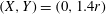 $(X,Y)=(0,1.4r)$
, (b)
$(X,Y)=(0,1.4r)$
, (b)
 $(X,Y)=(0,1.6r)$
and (c)
$(X,Y)=(0,1.6r)$
and (c)
 $(X,Y)=(0,1.62r)$
. The periodic orbit close to the relative equilibrium can exhibit oscillatory wave-like motion as in the absence of the flow (figure 6
a), but when the treadmiller is initially located at a larger separation from the wall, the trajectory can form a closed loop. The slight change in the initial position leads to swimming in the opposite direction, as illustrated in figure 6(b) (upstream migration) and figure 6(c) (downstream migration).
$(X,Y)=(0,1.62r)$
. The periodic orbit close to the relative equilibrium can exhibit oscillatory wave-like motion as in the absence of the flow (figure 6
a), but when the treadmiller is initially located at a larger separation from the wall, the trajectory can form a closed loop. The slight change in the initial position leads to swimming in the opposite direction, as illustrated in figure 6(b) (upstream migration) and figure 6(c) (downstream migration).
The relative equilibrium with
 $\unicode[STIX]{x03C0}/2<\unicode[STIX]{x1D703}<\unicode[STIX]{x03C0}$
, corresponding to swimming with
$\unicode[STIX]{x03C0}/2<\unicode[STIX]{x1D703}<\unicode[STIX]{x03C0}$
, corresponding to swimming with
 $\text{d}X/\text{d}t>0$
in the absence of a flow, however, does not disappear even when the shear strength is increased, which follows from the similar argument on the relative equilibrium with
$\text{d}X/\text{d}t>0$
in the absence of a flow, however, does not disappear even when the shear strength is increased, which follows from the similar argument on the relative equilibrium with
 $-\unicode[STIX]{x03C0}/2<\unicode[STIX]{x1D703}<0$
.
$-\unicode[STIX]{x03C0}/2<\unicode[STIX]{x1D703}<0$
.
When
 $\unicode[STIX]{x1D6FD}$
exceeds
$\unicode[STIX]{x1D6FD}$
exceeds
 $1/\sqrt{2}$
, another relative equilibrium bifurcates from infinity
$1/\sqrt{2}$
, another relative equilibrium bifurcates from infinity
 $(\unicode[STIX]{x1D70C}=0)$
with the angle
$(\unicode[STIX]{x1D70C}=0)$
with the angle
 $-\unicode[STIX]{x03C0}/2<\unicode[STIX]{x1D703}<-\unicode[STIX]{x03C0}/2$
. When a shear is applied to the swimmer with
$-\unicode[STIX]{x03C0}/2<\unicode[STIX]{x1D703}<-\unicode[STIX]{x03C0}/2$
. When a shear is applied to the swimmer with
 $1/\sqrt{2}<\unicode[STIX]{x1D6FD}<\infty$
, this relative equilibrium disappears at a lower shear strength than that discussed for the relative equilibrium with
$1/\sqrt{2}<\unicode[STIX]{x1D6FD}<\infty$
, this relative equilibrium disappears at a lower shear strength than that discussed for the relative equilibrium with
 $0<\unicode[STIX]{x1D703}<\unicode[STIX]{x03C0}$
, as this relative equilibrium is located further away from the wall. When
$0<\unicode[STIX]{x1D703}<\unicode[STIX]{x03C0}$
, as this relative equilibrium is located further away from the wall. When
 $\unicode[STIX]{x1D6FD}=\infty$
, the critical shear strength is again
$\unicode[STIX]{x1D6FD}=\infty$
, the critical shear strength is again
 $\unicode[STIX]{x1D6E4}_{\ast }=10-4\sqrt{6}$
, due to the symmetry.
$\unicode[STIX]{x1D6E4}_{\ast }=10-4\sqrt{6}$
, due to the symmetry.
7 Discussion
We have derived analytical expressions for the equations of motion of a circular treadmiller, with an arbitrary tangential velocity profile, near a no-slip wall in a simple shear. The governing dynamical equations are exact, and we have made no simplifying approximations. The mathematical approach made use of the reciprocal theorem of Stokes flow combined with a complex variable solution of a ‘dragging problem’ which greatly facilitated the evaluation of some integral expressions.
We demonstrated a Hamiltonian structure of the two-dimensional reduced dynamical system. With this symmetry, we found that the relative equilibria cannot be sources or sinks, but are always centres or saddles. As a result, the treadmiller is sensitive to external perturbations, which contrasts with the stable swimming of a spherical squirmer near a wall with constant separation from it (Ishimoto & Gaffney Reference Ishimoto and Gaffney2013). Stable swimming is only possible when the Hamiltonian symmetry is broken (such as in the case where weak fluid viscoelasticity is included (Yazdi et al. Reference Yazdi, Ardekani and Borham2015)). Wall potential forces, included in numerical studies (Ishikawa & Pedley Reference Ishikawa and Pedley2007; Spagnolie & Lauga Reference Spagnolie and Lauga2012; Ishimoto & Gaffney Reference Ishimoto and Gaffney2016), give rise to an additional velocity perpendicular to the wall given by
 $$\begin{eqnarray}{\mathcal{V}}_{ext}^{\prime }=\frac{1}{F_{y}}\left(-\frac{\unicode[STIX]{x2202}\unicode[STIX]{x1D719}}{\unicode[STIX]{x2202}y}\right),\end{eqnarray}$$
where
 $F_{y}$
is the perpendicular drag in the Jeffery–Onishi problem (3.23) and
$F_{y}$
is the perpendicular drag in the Jeffery–Onishi problem (3.23) and
 $\unicode[STIX]{x1D719}(y)$
is the external potential. This additional velocity breaks the Hamiltonian structure, and thus stable unidirectional swimming near the wall is possible, which may indicate that the swimmer behaviour depends on details of the swimmer–wall interactions, as examined for a spherical squirmer (Lintuvuori et al.
Reference Lintuvuori, Brown, Stratford and Marenduzzo2016). A gravitational potential can also be considered in the same manner, and the dynamics of a microswimmer with density offset such as green algae may be more stable (Drescher et al.
Reference Drescher, Leptos, Tuval, Pedley, Ishikawa and Goldstein2010).
$\unicode[STIX]{x1D719}(y)$
is the external potential. This additional velocity breaks the Hamiltonian structure, and thus stable unidirectional swimming near the wall is possible, which may indicate that the swimmer behaviour depends on details of the swimmer–wall interactions, as examined for a spherical squirmer (Lintuvuori et al.
Reference Lintuvuori, Brown, Stratford and Marenduzzo2016). A gravitational potential can also be considered in the same manner, and the dynamics of a microswimmer with density offset such as green algae may be more stable (Drescher et al.
Reference Drescher, Leptos, Tuval, Pedley, Ishikawa and Goldstein2010).
We studied the detailed motion of the treadmiller with the lowest two modes. Without a shear flow, as the swimmer parameter
 $\unicode[STIX]{x1D6FD}$
increases, two types of periodic orbit appear, associated with the bifurcation of relative equilibria of the reduced system. It is found that the swimming direction of oscillatory motion along the wall is determined by the sign of the Hamiltonian. When the shear is applied, the upstream oscillatory migration near the wall disappears at a critical shear strength. In contrast, the downstream oscillatory migration can be realized up to arbitrarily large shear strength, which indicates that shear flow can confine the swimmer near the wall with its orientation aligned. These results indicate that a simple shear near a wall can be used as a means to guide microswimmers with a particular swimming gait. They might also be useful in designing a microrobot (e.g. for drug-delivery) that would work in a vessel or an organ where a background flow is present.
$\unicode[STIX]{x1D6FD}$
increases, two types of periodic orbit appear, associated with the bifurcation of relative equilibria of the reduced system. It is found that the swimming direction of oscillatory motion along the wall is determined by the sign of the Hamiltonian. When the shear is applied, the upstream oscillatory migration near the wall disappears at a critical shear strength. In contrast, the downstream oscillatory migration can be realized up to arbitrarily large shear strength, which indicates that shear flow can confine the swimmer near the wall with its orientation aligned. These results indicate that a simple shear near a wall can be used as a means to guide microswimmers with a particular swimming gait. They might also be useful in designing a microrobot (e.g. for drug-delivery) that would work in a vessel or an organ where a background flow is present.
Acknowledgements
K.I. is supported by JSPS-KAKENHI for Young Researchers (15H06314), Kyoto University Hakubi Project and Kyoto University Supporting Program for Interaction-based Initiative Team Studies (SPIRIS). D.G.C. is supported by an EPSRC Established Career Fellowship EP/K019430/1 and a Royal Society Wolfson Research Merit Award. This work was initiated while D.G.C. was the SGU Distinguished Visiting Professor at Kyoto University in 2015–2016. The authors acknowledge Dr K. Obuse for fruitful discussions.


 Open access