


1. Introduction
Analyses and computations of colloidal particle electrophoresis in a liquid-filled circular cylinder usually assume that the cylinder is infinitely long (Keh & Anderson Reference Keh and Anderson1985; Keh & Chiou Reference Keh and Chiou1996; Yariv & Brenner Reference Yariv and Brenner2002, Reference Yariv and Brenner2003; Hsu & Yeh Reference Hsu and Yeh2007; Sherwood & Ghosal Reference Sherwood and Ghosal2018). The volumetric flow rate far from the particle is determined by the electroosmotic slip velocity created by the uniform electric field if the wall of the cylinder is charged (or is zero if the wall is uncharged). Misiunas et al. (Reference Misiunas, Pagliara, Lauga, Lister and Keyser2015) have shown that when the cylinder has finite length with open ends, Brownian motion of a particle creates a net liquid flow along the cylinder, leading to long-range particle–particle interactions within the cylinder. Similarly, if several particles are present within a cylinder or channel of finite length, electrophoresis is faster than for a single particle (Misiunas & Keyser Reference Misiunas and Keyser2019). We shall show that this too can be explained on the basis of a net volumetric flow along the cylinder. Other hydrodynamic interactions between the particles are expected to be weak once particles are separated by distances comparable to, or greater than, the cylinder diameter (Wang & Skalak Reference Wang and Skalak1969).
The aim of this paper is to determine the electrophoretic velocity of  $N$ identical spherical particles of radius $a$ along the axis of a liquid-filled cylinder of radius $R$ and of finite length $L$. The spheres fit tightly within the cylinder, i.e. $R-a=h_0\ll a$, and have uniform zeta potential $\zeta ^{s}$. The interior wall of the cylinder has uniform zeta potential $\zeta ^{c}$, and, far from the spheres, the imposed electric field $\boldsymbol E_0$ (with magnitude $E_0$) is aligned parallel to the axis of the cylinder. The incompressible liquid has viscosity $\mu$ and electrical permittivity $\epsilon _ l$, and the number density of ions within the liquid is sufficiently high that the Debye length $\kappa ^{-1}$, which characterizes the thickness of the charge cloud of counter-ions adjacent to any charged surface, is small compared with the gap width $h_0$. The electrophoretic velocity of the sphere in unbounded liquid is given by the Smoluchowski velocity $\epsilon _l\boldsymbol E_0\zeta ^{s}/\mu$. The electroosmotic velocity of liquid within an infinite cylinder would be $-\epsilon _l\boldsymbol E_0\zeta ^{c}/\mu$, so that if the spherical particle were small compared with the cylinder radius its observed velocity would be
 \begin{equation} U_{Smol}= \epsilon_l\boldsymbol E_0(\zeta^{s}-\zeta^{c})/\mu.\end{equation}
Electrophoretic velocities are usually small, as are colloidal particles. For example, in the experiments of Misiunas & Keyser (Reference Misiunas and Keyser2019) the electrophoretic velocity was typically  $17\ \mathrm {\mu }\text {m s}^{-1}$ and the particle diameter was $2a=505\ \textrm {nm}$. We therefore assume that Reynolds numbers are small, so that liquid motion is governed by the Stokes equations.
Our strategy is to first determine the pressure difference  ${\rm \Delta} p$, generated by the electrophoretic motion, between liquid in front of and behind a single tightly fitting sphere. In an infinitely long cylinder this pressure difference has no effect upon the infinite columns of liquid within the cylinder. But in a cylinder of finite length, opening into reservoirs with fixed pressure, the pressure difference causes motion of the liquid, thereby enhancing the observed electrophoretic velocity. If there are several spheres within the cylinder, the pressure-generated motion and the velocities of the spheres are further enhanced, as has been observed experimentally by Misiunas & Keyser (Reference Misiunas and Keyser2019).
Sherwood & Ghosal (Reference Sherwood and Ghosal2018) used a lubrication analysis to determine the electrophoretic velocity of a tightly fitting sphere inside an infinite cylinder. They found a pressure difference  ${\rm \Delta} p$ which was nominally $O((R/h_0)^{5/2})$, whereas the total force due to wall shear stresses was $O((R/h_0)^{3/2})$. A force balance on a cylindrical control volume containing the spherical particle was impossible in the limit $h_0/R\rightarrow 0$, unless the leading-order pressure difference ${\rm \Delta} p$ vanished, which required the electrophoretic velocity of the sphere to be $U_{Smol}/2$. This is the electrophoretic velocity in the limit $h_0/R\rightarrow 0$ determined analytically by Yariv & Brenner (Reference Yariv and Brenner2003) and numerically by Keh & Chiou (Reference Keh and Chiou1996).
This limit leaves us with  ${\rm \Delta} p=0$ and no possibility of predicting pressure-driven motion within a cylinder of finite length. We therefore embark upon a higher-order lubrication analysis of the flow (Bungay & Brenner Reference Bungay and Brenner1973). The leading-order analysis is similar to that of Yariv & Brenner (Reference Yariv and Brenner2003), who considered a sphere at an arbitrary radial position, rather than on the centreline of the cylinder. They split the velocity field into the irrotational flow due to a uniform potential $\zeta ^{c}$ on both the cylinder and sphere, and an additional velocity due to a potential $\zeta ^{s}-\zeta ^{c}$ on the sphere alone. The leading-order force on the sphere due to this additional velocity was evaluated by means of the reciprocal theorem and an integral over the surface of the sphere. Contributions to this integral from higher terms in the expansion of the electric potential were zero, so there was no need to determine these higher terms. Here, we shall continue our analysis to second order and predict a non-zero pressure difference ${\rm \Delta} p$ when $h_0/R$ is small but non-zero. We shall then turn to more physically based arguments to determine the motion of $N$ identical spheres along the cylinder.
The geometry is axisymmetric: we use cylindrical polar coordinates  $(r,z)$, with the $z$ axis aligned along the axis of the cylinder, and with the centre of the sphere on the plane $z=0$, as seen in figure 1. We shall also use $x=R-r$ as a coordinate normal to the inner surface of the cylinder. A potential difference $V$ is applied across the ends of the cylinder, such that the electric field is $\boldsymbol E_0 =E_0\hat {\boldsymbol z}$ within the cylinder far from the sphere.

Figure 1. A single charged sphere of radius  $a$ in a liquid-filled circular cylinder of radius $R=a+h_0$, with $h_0\ll R$. The electrophoretic velocity of the sphere is $U$, and the imposed electric field has strength $E_0$ away from the sphere.
The surface of the sphere is at  $(r,z)=a(\cos \theta,\sin \theta )$ where $\theta$ is a spherical polar coordinate with $\theta =0$ in the plane $z=0$. The gap width $h$ is therefore
 \begin{equation} \frac{h}{a}=\frac{R-a}{a}+\frac{z^2}{2a^2}+\frac{z^4}{8a^4}+\cdots. \end{equation}
We follow Bungay & Brenner (Reference Bungay and Brenner1973) and Yariv & Brenner (Reference Yariv and Brenner2003) and set  $x=R-r$, $\epsilon =(R-a)/a=h_0/a$, $X=x/(a\epsilon )$, $H=h/(a\epsilon )$ and $Z=z/(a\epsilon ^{1/2})$, so that
 \begin{equation} \frac{h}{a}=\epsilon+\epsilon\frac{Z^2}{2}+\epsilon^2\frac{Z^4}{8}+\cdots, \end{equation}
and
 \begin{equation} H=1+\frac{Z^2}{2}+\epsilon\frac{Z^4}{8}+\cdots\quad \equiv H_0+\epsilon H_1+\cdots.\end{equation}
Note that  $R=a(1+\epsilon )$ and $r=R-x=a(1+\epsilon -\epsilon X)$.
2. The electric field in the narrow gap
We have to solve the Laplace equation for the potential  $\phi$, which is axisymmetric,
 \begin{equation} \left[\frac{1}{r}\frac{\partial}{\partial r} r \frac{\partial}{\partial r} +\frac{\partial^2}{\partial z^2}\right]\phi=0, \end{equation}
i.e.
 \begin{equation} \left[\frac{1}{\epsilon^2(1+\epsilon-\epsilon X)}\frac{\partial}{\partial X} (1+\epsilon-\epsilon X) \frac{\partial}{\partial X} +\frac{1}{\epsilon}\frac{\partial^2}{\partial Z^2}\right]\phi=0.\end{equation}
The surface conduction of a plane charge cloud adjacent to a surface at potential  $\zeta _0$ is negligible compared with that of the electrolyte-filled gap of width $h$ if $\exp (e\zeta _0/2kT)\ll \kappa h$, where $e$ is the charge on a proton and $kT$ is the Boltzmann temperature. We assume that both $\zeta ^{c}$ and $\zeta ^{s}$ satisfy this condition, since $\kappa h\gg 1$, and surface conduction can indeed be neglected. There can therefore be no flux of current normal to the surfaces of the sphere and cylinder, where the normal component of the electric field must be zero. The potential $\phi$ therefore satisfies the boundary conditions
 $$\begin{gather} \frac{\partial\phi}{\partial X}=0\quad \hbox{on } X=0, \end{gather}$$
 $$\begin{gather}\boldsymbol n\boldsymbol{\cdot} \boldsymbol{\nabla}\phi=0 \quad\hbox{on } X=H, \end{gather}$$
where  $\boldsymbol n$ is the normal to the surface of the sphere, which is described by $x-h(z)=0$. The normal $\boldsymbol n=\boldsymbol {\nabla }(x-h(z))$ is therefore
 \begin{align} \boldsymbol n=(n_x,n_z)=(1,-\partial_zh)=(1,-z/a-z^3/(2a^3)+\cdots) =(1,-\epsilon^{1/2}[Z+\epsilon Z^3/2+\cdots]).\end{align}
But  $n_x\partial _x\phi +n_z\partial _z\phi =0$ implies $n_x\epsilon ^{-1}\partial _X\phi +n_z\epsilon ^{-1/2}\partial _Z\phi =0$, so we require
 \begin{equation} \frac{\partial \phi}{\partial X}-\epsilon(Z+\epsilon Z^3/2+\cdots) \frac{\partial \phi}{\partial Z}=0, \quad \hbox{on } X=H.\end{equation}
 We seek solutions for the electrical potential and liquid velocities that can be expanded in powers of the small parameter  $\epsilon$, and we shall make all such expansions non-dimensional. We therefore look for a non-dimensional expansion of $\phi$ of the form
 \begin{equation} \phi=\epsilon^{{-}1/2}\left(\frac{E_0R^2}{a}\right)(\phi_0 +\epsilon\phi_1+\cdots).\end{equation}
A factor  $R^2/a$ enters naturally later in the analysis when the electric field is evaluated from the total flux across the cross-section of the cylinder, and it is convenient to include this factor in the definition of the expansion (2.6). The Laplace equation (2.2) becomes
 \begin{equation} \left[\frac{\partial}{\partial X} (1+\epsilon-\epsilon X) \frac{\partial}{\partial X} +\epsilon(1+\epsilon-\epsilon X)\frac{\partial^2}{\partial Z^2}\right] (\phi_0+\epsilon\phi_1+\cdots)=0.\end{equation}
At leading order
 \begin{equation} \frac{\partial^2\phi_0}{\partial X^2} =0, \end{equation}
and since  $\partial \phi /\partial X=0$ on $X=0$, we conclude that $\phi _0$ is independent of $X$. We follow Yariv & Brenner (Reference Yariv and Brenner2003) and determine $\phi _0$ by appealing to conservation of the total flux of the electric field (and current), which is easily evaluated to be ${\rm \pi} R^2E_0$ far from the sphere, so that
 \begin{equation} 2{\rm \pi} \int_a^R r\frac{\partial \phi}{\partial z}\,\textrm{d}r={-}{\rm \pi} R^2E_0, \end{equation}
i.e.
 \begin{equation} \int_0^H (1+\epsilon-\epsilon X)\frac{\partial }{\partial Z} (\phi_0 +\epsilon\phi_1+\cdots)\,\textrm{d}X={-}1/2. \end{equation}
Hence
 \begin{equation} \left\{ (1+\epsilon)\left(1+\frac{{Z}^2}{2}+\epsilon\frac{{Z}^4}{8}\right) -\frac{\epsilon}{2}\left(1+\frac{{Z}^2}{2}+\epsilon\frac{{Z}^4}{8}\right)^2 \right\} \frac{\textrm{d}\phi_0}{\textrm{d}Z} +\int_0^H\epsilon \frac{\partial \phi_1}{\partial Z}\,\textrm{d}X ={-}\frac{1}{2}.\end{equation}
At leading order
 \begin{equation} \frac{\textrm{d}\phi_0}{\textrm{d}Z}={-}\frac{1}{2(1+Z^2/2)},\end{equation}
and hence
 \begin{equation} \phi_0={-}\frac{1}{2^{1/2}}\tan^{{-}1}\left(\frac{Z}{\sqrt 2}\right), \end{equation}
as found by Yariv & Brenner (Reference Yariv and Brenner2003) when the sphere is on the axis of the cylinder. Thus to leading order the change in electrical potential across the particle is
 \begin{equation} {\rm \Delta}\phi=[\phi_0(\infty)-\phi_0(-\infty)] \frac{E_0R^2}{a\epsilon^{1/2}}={-}\frac{{\rm \pi} E_0R^2 }{(2ah_0)^{1/2}}.\end{equation}
The second-order terms in the Laplace equation (2.7) are
 \begin{equation}
\frac{\partial^{2}\phi_1}{\partial X^{2}}={-}\frac{\textrm{d}^{2} \phi_{0}}{\textrm{d}Z^{2}}=
-\frac{Z}{2(1+Z^2/2)^{2}},\end{equation}
\begin{equation}
\frac{\partial^{2}\phi_1}{\partial X^{2}}={-}\frac{\textrm{d}^{2} \phi_{0}}{\textrm{d}Z^{2}}=
-\frac{Z}{2(1+Z^2/2)^{2}},\end{equation}
subject to boundary conditions  $\partial _X\phi _1=0$ on $X=0$ and, by (2.5),
 \begin{equation} \frac{\partial\phi_1 }{\partial X}=Z \frac{\textrm{d}\phi_0}{\textrm{d}Z}={-}\frac{Z}{2(1+Z^2/2)},\quad \hbox{on } X=H. \end{equation}
The governing equation (2.15) and boundary conditions for  $\phi _1$ were given by Yariv & Brenner (Reference Yariv and Brenner2003), but $\phi _1$ was not required for their leading-order evaluation of the force on the sphere, and so was not determined explicitly. Integrating (2.15) once gives
 \begin{equation} \frac{\partial\phi_1 }{\partial X}={-}\frac{Z}{2(1+Z^2/2)^2}X+f(Z),\end{equation}
and the boundary condition  $\partial _X\phi =0$ on $X=0$ implies that the unknown function of integration $f(Z)=0$. If we evaluate $\partial _X\phi _1$ (2.17) on $X=H$,
 \begin{equation} \frac{\partial\phi_1}{\partial X}={-}\frac{Z}{2(1+Z^2/2)^2}\left(1+\frac{Z^2}{2}+\cdots\right),\quad X=H, \end{equation}
we see that the boundary condition (2.16) is satisfied. Integrating (2.17),
 \begin{equation} \phi_1={-}\frac{Z}{2(1+Z^2/2)^2}\frac{X^2}{2}+g(Z),\end{equation}
where  $g(Z)$ is as yet unknown. The flux condition (2.11) gives, at second order,
 \begin{equation} \frac{1}{2}\frac{\textrm{d}\phi_0}{\textrm{d}Z}+\int_0^H \frac{\partial\phi_1}{\partial Z}\,\textrm{d}X=0. \end{equation}
Hence
 \begin{equation} -\frac{1}{4(1+Z^2/2)} ={-}\frac{\textrm{d}g(Z)}{\textrm{d}Z}\left(1+\frac{Z^2}{2}\right)+\frac{H^3}{12} \left[ \frac{1-3Z^2/2}{(1+Z^2/2)^3}\right], \end{equation}
i.e.
 \begin{equation} \frac{\textrm{d}g(Z)}{\textrm{d}Z} \left(1+\frac{Z^2}{2}\right) = \frac{(4-Z^2-3Z^4/4)}{12(1+Z^2/2)}. \end{equation}
Hence, differentiating (2.19),
 \begin{equation} \frac{\partial\phi_1}{\partial Z} = \left[-\frac{(1-3Z^2/2)X^2}{4(1+Z^2/2)^3} + \frac{(4-Z^2-3Z^4/4)}{12(1+Z^2/2)^2} \right],\end{equation}
and we see that as  $Z\rightarrow \infty$ the dimensional electric field is
 \begin{equation} -\frac{\partial }{\partial z} (\epsilon^{1/2}\phi_1) \frac{R^2E_0}{a} ={-}\frac{\partial\phi_1 }{\partial Z}\frac{R^2E_0}{a^2}={-}\frac{R^2E_0}{4a^2}. \end{equation}
Thus our expansion does not match to the uniform electric field far from the gap, and we have no analytic solution to which the lubrication analysis might be matched in some intermediate zone. Our analysis is therefore closer to an extended lubrication analysis (cf. Tavakol et al. Reference Tavakol, Froehlicher, Holmes and Stone2017), rather than to one based on matched asymptotic expansions. However, the hydrodynamic problem is strongly dominated by the region of the narrow gap (more so than the electrostatic problem), and a solution in the narrow gap is all that we shall need.
3. Liquid motion within the narrow gap
3.1. The Smoluchowski slip boundary conditions
The electric field is tangential to the insulating surfaces of the sphere and cylinder, and creates motion of the liquid within the charge cloud adjacent to the surface. If the surface has potential  $\zeta _0$, liquid just outside the charge cloud appears to slip relative to the surface with the Smoluchowski slip velocity
 \begin{equation} u_{tan}={-}\frac{\epsilon_l\zeta_0}{\mu}E_{tan},\end{equation}
where  $E_{tan}$ is the tangential electric field. We have ensured that the electric field $\boldsymbol E$ satisfies $\boldsymbol n\boldsymbol {\cdot } \boldsymbol E=0$ on the boundaries of the sphere and cylinder, so if we impose $\boldsymbol u=-\epsilon _l\zeta \boldsymbol E/\mu$ on these surfaces (with $\zeta =\zeta ^{c}$ or $\zeta ^{s}$ as appropriate), we ensure that both the Smoluchowski slip condition (3.1) and the zero normal velocity condition $\boldsymbol n\boldsymbol {\cdot } \boldsymbol u=0$ are satisfied. We non-dimensionalize surface potentials by the arbitrary potential $\zeta _0$, setting
 \begin{equation} \widehat{\zeta^{c}}=\zeta^{c}/\zeta_0,\quad \widehat{\zeta^{s}}=\zeta^{s}/\zeta_0, \end{equation}
and for ease of notation we use  $(u^{c},v^{c})$ and $(u^{s},v^{s})$ to denote the $(z,r)$ components of the slip velocities on the cylinder and sphere, respectively, with
 \begin{equation} u^{c}=\frac{\epsilon_l\zeta^{c}}{\mu}\frac{\partial\phi }{\partial z} =\frac{\widehat{\zeta^{c}}}{\epsilon}\left(\frac{\zeta_0\epsilon_lR^2E_0}{\mu a^2}\right) \frac{\partial }{\partial Z} (\phi_0+\epsilon\phi_1+\cdots). \end{equation}
Motivated by (3.3), we non-dimensionalize the expansion of velocities by the velocity scale
 \begin{equation} u_{scale}=\zeta_0\epsilon_lR^2E_0/(\mu a^2), \end{equation}
and that of pressure (and stress) by  $\mu u_{scale}/a$. Expansions for volumetric flow rates will be non-dimensionalized by $a^2u_{scale}$, and those for force (e.g. over the area of a control volume) by $\mu au_{scale}$. On the cylindrical boundary we therefore adopt the expansion
 \begin{equation} u=u^{c} =\epsilon^{{-}1}u_{scale} \{ u^{c}_0+\epsilon u^{c}_1+\cdots\},\end{equation}
where, by (2.12),
 \begin{equation} u^{c}_0={-}\widehat{\zeta^{c}}\frac{\textrm{d}\phi_0}{\textrm{d}Z} ={-}\frac{\widehat{\zeta^{c}}}{2(1+Z^2/2)}.\end{equation}
By (2.23) with  $X=0$,
 \begin{equation} u^{c}_1 =\widehat{\zeta^{c}}\frac{\partial\phi_1}{\partial Z} =\widehat{\zeta^{c}}\frac{(4-Z^2-3Z^4/4)}{12(1+Z^2/2)^2}.\end{equation}
The slip velocity on the sphere is, like (3.5), expanded as
 \begin{equation} u(X=H)=u^{s} =\epsilon^{{-}1}u_{scale} \{ u^{s}_0+\epsilon u^{s}_1+\cdots\}, \end{equation}
with
 \begin{equation} u_0^{s}={-}\frac{\hat\zeta^{s}}{2(1+Z^2/2)}. \end{equation}
We shall discuss the next-order correction  $u_1^{s}$ to the slip velocity on the sphere in § 3.5.
3.2. Governing equations
The equation of continuity in cylindrical polars  $(r,z)$, for an axisymmetric flow field $(v,u)$, is
 \begin{equation} \frac{\partial }{\partial r} (rv)+r \frac{\partial u}{\partial z}=0.\end{equation}
The Stokes equations are
 \begin{equation} \frac{1}{\mu}\frac{\partial p}{\partial r}=\nabla^2 v-\frac{v}{r^2}=\frac{1}{r}\frac{\partial }{\partial r} \left(r\frac{\partial v}{\partial r}\right) +\frac{\partial^2v }{\partial z^2}-\frac{v}{r^2}, \end{equation}
and
 \begin{equation} \frac{1}{\mu}\frac{\partial p}{\partial z}=\nabla^2 u =\frac{1}{r}\frac{\partial }{\partial r} \left(r \frac{\partial u}{\partial r}\right)+\frac{\partial^2 u}{\partial z^2}. \end{equation}
We again set  $r=R-x$, $X=x/(a\epsilon )$, $Z=z/(a\epsilon ^{1/2})$, $r=a(1+\epsilon -\epsilon X)$. The equation of continuity (3.10) becomes
 \begin{equation} -\frac{1}{\epsilon}\frac{\partial }{\partial X}[(1+\epsilon-\epsilon X)v]+\frac{(1+\epsilon-\epsilon X)}{\epsilon^{1/2}}\frac{\partial u}{\partial Z}=0. \end{equation}
We see that  $v$ is smaller than $u$, and we therefore look for non-dimensional expansions
 $$\begin{gather} u=\epsilon^{{-}1}u_{scale}\{ u_0+\epsilon u_1+\cdots\}, \end{gather}$$
 $$\begin{gather}v={-}\epsilon^{{-}1/2} u_{scale}\{ v_1+\cdots\}, \end{gather}$$
 $$\begin{gather}p=\epsilon^{{-}5/2}\left(\frac{\mu u_{scale}}{a}\right) \{ p_0+\epsilon p_1+\cdots\}. \end{gather}$$
Note that we have chosen the sign of the expansion of  $v$ such that $v_1>0$ corresponds to flow in the $x$ direction, inwards from the wall of the cylinder, rather than in the $r$ direction.
The equation of continuity (3.13) becomes, at leading order,
 \begin{equation} \frac{\partial v_1}{\partial X}+\frac{\partial u_0}{\partial Z}=0.\end{equation}
The Stokes equation for the axial velocity  $u$ (3.12) becomes
 \begin{equation} \frac{(1+\epsilon-\epsilon X)} {\epsilon^{1/2}\mu}\frac{\partial p}{\partial Z}=\frac{1}{a\epsilon^2}\frac{\partial }{\partial X}\left[ (1+\epsilon-\epsilon X) \frac{\partial u}{\partial X}\right]+\frac{(1+\epsilon-\epsilon X)}{a\epsilon}\frac{\partial^2u }{\partial Z^2}. \end{equation}
At leading order
 \begin{equation} \frac{\partial p_0}{\partial Z}=\frac{\partial^2u_0}{\partial X^2}.\end{equation}
At second order, equating the coefficients of  $\epsilon ^{-5/2}$ in (3.16) gives
 \begin{equation} \left[ \frac{\partial p_1}{\partial Z}+(1-X) \frac{\partial p_0}{\partial Z} \right] =\frac{\partial^2u_1}{\partial X^2} +\frac{\partial^2 u_0}{\partial Z^2} +(1-X) \frac{\partial^2 u_0}{\partial X^2}-\frac{\partial u_0}{\partial X}, \end{equation}
which simplifies immediately to give
 \begin{equation} \frac{\partial p_1}{\partial Z} =\frac{\partial^2u_1}{\partial X^2}+\frac{\partial^2u_0}{\partial Z^2}-\frac{\partial u_0}{\partial X}.\end{equation}
The leading-order Stokes equation (3.11) for  $v$ is
 \begin{equation} -\frac{a}{\mu\epsilon}\frac{\partial p}{\partial X}=\frac{1}{\epsilon^2}\frac{\partial^2v}{\partial X^2} +\frac{1}{\epsilon}\frac{\partial^2 v}{\partial Z^2}-v,\end{equation}
and we conclude from the leading-order  $\epsilon ^{-7/2}$ term
 \begin{equation} \frac{\partial p_0}{\partial X}=0,\end{equation}
so that  $p_0$ is a function of $Z$ alone. At the next order, equating the coefficients of $\epsilon ^{-5/2}$, (3.20) gives
 \begin{equation} \frac{\partial p_1}{\partial X}=\frac{\partial^2v_1}{\partial X^2}, \end{equation}
so that
 \begin{equation} p_1=\frac{\partial v_1}{\partial X}+F(Z), \end{equation}
for some as yet unknown function of integration  $F(Z)$.
The velocity normal to the solid surfaces must be zero. This immediately gives
 \begin{equation} v=0\quad \hbox{on } X=0. \end{equation}
The normal to the surface of the sphere is given by (2.4) and leads to the condition
 \begin{equation} -\epsilon^{{-}1/2}v_1+\epsilon^{{-}1/2}(Z+\epsilon Z^3/2)(u_0+\epsilon u_1)=0. \end{equation}
Hence, on the sphere,
 \begin{equation} v_1=Zu_0.\end{equation}
 If  $\zeta ^{s}=\zeta ^{c}$ the irrotational velocity field $\boldsymbol u=-\zeta ^{s}\epsilon _l\boldsymbol E/\mu$, with the sphere at rest, satisfies both the flow equations and the boundary conditions, and hence the electrophoretic velocity $U$ of the sphere is zero. We have assumed that charge clouds are sufficiently thin so that the slip velocity at each boundary depends linearly on its zeta potential. We therefore expect the electrophoretic velocity to depend linearly on both $\zeta ^{s}$ and $\zeta ^{c}$ and to take the form $U=\alpha \zeta ^{s}+\beta \zeta ^{c}$ for some as yet unknown $\alpha$ and $\beta$. Only if $\alpha =-\beta$ will $U$ be zero when $\zeta ^{s}=\zeta ^{c}$ and hence $U$ must be proportional to $\zeta ^{s}-\zeta ^{c}$ for all values of $a/R$, and not just for $a\ll R$ (1.1). This will be a useful check on analytic predictions.
3.3. The leading-order axial velocity  $u_0$
$u_0$

We assume that the sphere moves along the cylinder with a velocity  $U$ that can be expanded as
 \begin{equation} U=u_{scale}\{ U_0+\epsilon U_1+\cdots\},\end{equation}
where we have adopted our usual velocity scale  $u_{scale}$ (3.4) for non-dimensionalization of the series expansion of $U$, and we note that this expansion (3.27) starts at $O(1)$, whereas the expansion (3.14a) for the liquid velocity $u$ starts at $O(\epsilon ^{-1})$, since liquid has to squeeze through the narrow gap between the sphere and cylinder wall.
Far away from the sphere, the electric field  $E_0$ generates a uniform electroosmotic velocity $-\epsilon _l\zeta ^{c}E_0/\mu$ leading to a volumetric flow rate $-{\rm \pi} R^2\epsilon _l\zeta ^{c}E_0/\mu$, and we shall non-dimensionalize all volumetric flow rates by $a^2u_{scale} =\epsilon _l\zeta _0E_0R^2/\mu$. When we later discuss motion in cylinders of finite length, we shall allow for the possibility of an additional pressure-driven volumetric flow rate $Q_L$ in the laboratory frame. We know from previous work (Sherwood & Ghosal Reference Sherwood and Ghosal2018) that in the limit $\epsilon =0$ there is no pressure difference across the sphere, and hence no pressure-driven flow. In consequence, we expect
 \begin{equation} Q_L=a^2u_{scale}\{\epsilon Q_{L1}+\cdots\}.\end{equation}
We now move into the frame of reference which moves with the sphere, so that the total volumetric flow rate in the frame in which the sphere is at rest is
 \begin{align} Q &= Q_{L} -{\rm \pi} R^2\left(\frac{\epsilon_l\zeta^{c}}{\mu}E_0+U\right) \nonumber\\ &=\left(\frac{\epsilon_l\zeta_0E_0R^2}{\mu}\right)\left\{ \epsilon Q_{L1} -{\rm \pi} \widehat{\zeta^{c}} -\frac{{\rm \pi} R^2}{a^2}(U_0+\epsilon U_1)+\cdots\right\} \nonumber\\ &=\left(\frac{\epsilon_l\zeta_0E_0R^2}{\mu}\right)\{ Q_0+\epsilon Q_1+\cdots\}, \end{align}
so that
 \begin{equation} Q_0={-}{\rm \pi} \left(\widehat{\zeta^{c}}+\frac{R^2}{a^2}U_0\right),\quad Q_1=\left(Q_{L1}-\frac{{\rm \pi} R^2}{a^2} U_1\right). \end{equation}
Note that in this frame the liquid velocity at the cylindrical wall is  $u=u^{c}-U$, which in terms of the non-dimensional series expansions becomes
 \begin{equation} \epsilon^{{-}1} \{ u_0+\epsilon u_1+\cdots\} =\epsilon^{{-}1}\{ u^{c}_0+\epsilon u^{c}_1+\cdots\} -\{ U_0+\epsilon U_1+\cdots\},\quad \hbox{on } X=0.\end{equation}
We see that at  $O(\epsilon ^{-1})$ this change in frame of reference makes no difference to the boundary condition for $u_0$ at the cylinder wall.
We first integrate the Stokes equation (3.17) to obtain
 \begin{align} u_0&=\frac{\textrm{d}p_0 }{\textrm{d}Z } \frac{X(X-H_0)}{2}+u_0^{c}+\frac{(u_0^{s}-u_0^{c})X}{H_0}, \end{align}
 \begin{align} &=\frac{\textrm{d}p_0 }{\textrm{d}Z } \frac{X(X-1-Z^2/2)}{2}-\frac{\hat\zeta^{c}}{2(1+Z^2/2)}- \frac{(\hat\zeta_0^{s}-\hat\zeta_0^{c})X}{2(1+Z^2/2)^2}. \end{align}
This solution for  $u_0$ satisfies the Smoluchowski slip boundary conditions (to leading order) at the bounding surfaces of the cylinder and sphere. The unknown pressure gradient $\partial _Zp_0$ is a function of $Z$ alone, by (3.21). It is found by considering the total volumetric flow through the gap between the sphere and cylinder, which is
 \begin{equation} Q=2{\rm \pi} \int_h^R ru\,\textrm{d}r =2{\rm \pi} \epsilon a^2u_{scale}\int_0^H(1+\epsilon-\epsilon X) \frac{(u_0+\epsilon u_1+\cdots)}{\epsilon}\,\textrm{d}X. \end{equation}
In terms of the non-dimensional expansion (3.29)
 \begin{align} \frac{Q_0}{2{\rm \pi} }+\epsilon \frac{Q_1}{2{\rm \pi} }&=\int_0^H u_0\,\textrm{d}X+\epsilon\int_0^H[ (1-X)u_0+u_1]\,\textrm{d}X\nonumber\\ &=\int_0^{H_0} u_0\,\textrm{d}X +\epsilon\int_0^{H_0}[(1-X)u_0+u_1]\,\textrm{d}X +\epsilon H_1 u_0(H). \end{align}
At leading order, using (3.32a)
 \begin{equation} \frac{Q_0}{2{\rm \pi} }=\int_0^{H_0} u_0\,\textrm{d}X ={-}\frac{\textrm{d}p_0}{\textrm{d}Z}\frac{H_0^3}{12}+u_0^{c}H_0+(u_0^{s}-u_0^{c})\frac{H_0}{2}, \end{equation}
so that, by (3.30a,b),
 \begin{equation} \frac{\textrm{d}p_0}{\textrm{d}Z}=\frac{12}{H_0^3}\left\{ (u_0^{s}+u_0^{c})\frac{H_0}{2} -\frac{Q_0}{2{\rm \pi} }\right\} ={-}(\hat\zeta^{c}+\hat\zeta^{s})\frac{3}{H_0^3} +6\frac{\hat\zeta^{c}}{H_0^3}+\frac{6 R^2U_0}{a^2 H_0^3}.\end{equation}
 We consider the forces on a cylindrical control volume, which we choose with axis along  $r=0$, plane ends at $\pm |z|\gg a$ and with radius slightly smaller than $R$, so that the interior is electrically neutral (since the charge cloud adjacent to the cylinder is excluded, and the sphere is surrounded by its cloud of counter-ions). The pressure forces on the two plane ends contribute a non-dimensional force in the $z$ direction with leading order
 \begin{align} - \frac{{\rm \pi} R^2}{a^2\epsilon^{5/2}}\int_{-\infty}^\infty \frac{\textrm{d}p_0}{\textrm{d}Z}\textrm{d}Z&={-} \frac{{\rm \pi} R^2}{ a^2\epsilon^{5/2}} \left[\hat\zeta^{c}-\hat\zeta^{s}+\frac{2R^2}{a^2}U_0\right]\int_{-\infty}^\infty \frac{\textrm{d}Z}{(1+Z^2/2)^3} \nonumber\\ &={-}\frac{{\rm \pi} R^2}{a^2\epsilon^{5/2}} \left[ \hat\zeta^{c}-\hat\zeta^{s}+\frac{2R^2}{a^2}U_0\right] \frac{3\sqrt 2{\rm \pi} }{8}. \end{align}
The leading-order shear stress is
 \begin{equation} \tau_{zx} =\mu \frac{\partial u}{\partial x}=\frac{\mu u_{scale}}{a\epsilon^2}\frac{\partial u_0 }{\partial X} =\frac{\mu u_{scale}}{a\epsilon^2}\left[ \frac{\textrm{d}p_0}{\textrm{d}Z} (X-H_0/2)+\frac{(u_0^{s}-u_0^{c})}{H_0} \right]. \end{equation}
On  $X=0^+$ (i.e. just outside the charge cloud adjacent to the cylinder) this is
 \begin{align} \tau_{zx}=\frac{\mu u_{scale}}{a\epsilon^2}\left\{ \left[ \hat\zeta^{s}-\hat\zeta^{c}-\frac{2R^2}{a^2}U_0\right] \frac{3}{2H_0^2} -\frac{(\hat\zeta^{s}-\hat\zeta^{c})}{2H_0^2}\right\} =\frac{\mu u_{scale}}{a\epsilon^2H_0^2} \left[ \hat\zeta^{s} -\hat\zeta^{c}-3\frac{R^2}{a^2}U_0\right]. \end{align}
The total force acting on the curved surface of the control volume, in the  $z$ direction, is
 \begin{equation} -2{\rm \pi} R\int_{-\infty}^{\infty}\tau_{xz}\,\textrm{d}z ={-}\frac{2{\rm \pi} R\mu u_{scale}}{\epsilon^{3/2}}\left[ \hat\zeta^{s} -\hat\zeta^{c}-3\frac{R^2}{a^2}U_0\right] \int_{-\infty}^{\infty}\frac{\textrm{d}Z}{(1+Z^2/2)^2}.\end{equation}
We see that the force on the control volume due to pressure at the plane ends is  $O(\epsilon ^{-5/2})$, whereas that due to the shear stress over the curved cylindrical surface is $O(\epsilon ^{-3/2})$. No balance is possible unless $\textrm {d}p_0/\textrm {d}Z=0$. We conclude from (3.37) that
 \begin{equation} U_0=\frac{a^2}{2R^2}(\hat\zeta^{s}-\hat\zeta^{c}), \end{equation}
so that, to leading order, the dimensional electrophoretic velocity is
 \begin{equation} U=\frac{\epsilon_l (\zeta^{s}-\zeta^{c})E_0}{2\mu},\end{equation}
as found by Yariv & Brenner (Reference Yariv and Brenner2003), and the leading-order pressure gradient (3.36) and total pressure force (3.37) are zero. The leading-order liquid velocity (3.32b) reduces to
 \begin{equation} u_0={-}\frac{\hat\zeta^{c}}{2(1+Z^2/2)}- \frac{(\hat\zeta^{s}-\hat\zeta^{c})X}{2(1+Z^2/2)^2},\end{equation}
and the leading-order force on the cylindrical surface of the control volume (3.40) due to shear stress is
 \begin{equation} -2{\rm \pi} R\int_{-\infty}^{\infty}\tau_{xz}\,\textrm{d}z =\frac{{\rm \pi} R\mu u_{scale}}{\epsilon^{3/2}}[ \hat\zeta^{s} -\hat\zeta^{c}] \frac{\sqrt 2{\rm \pi} }{2}.\end{equation}
3.4. Leading-order radial velocity $v_1$

We can now obtain  $v_1$ from the equation of continuity (3.15)
 \begin{equation} \frac{\partial v_1}{\partial X}={-}\frac{\partial u_0}{\partial Z} ={-}\frac{\hat\zeta^{c}Z}{2(1+Z^2/2)^2}-(\hat\zeta^{s}-\hat\zeta^{c})\frac{ZX}{(1+Z^2/2)^3}. \end{equation}
Integrating, and using the result  $v=0$ on $X=0$,
 \begin{equation} v_1={-}\frac{\hat\zeta^{c}ZX}{2(1+Z^2/2)^2}-(\hat\zeta^{s}- \hat\zeta^{c})\frac{ZX^2}{2(1+Z^2/2)^3}.\end{equation}
On  $X=H$ this becomes
 \begin{equation} v_1={-}\frac{\hat\zeta^{c}Z}{2(1+Z^2/2)}-(\hat\zeta^{s}-\hat\zeta^{c})\frac{Z}{2(1+Z^2/2)}, \end{equation}
and we see, by comparison with (3.32b), that  $v_1=Zu_0$ on $X=H$, as required by the boundary condition (3.26).
Having found  $v_1$ (3.46), we obtain $p_1$ (3.23) as
 \begin{align} p_1&=\frac{\partial v_1}{\partial X}+F(Z) \end{align}
 \begin{align} &={-}\frac{\hat\zeta^{c}Z}{2(1+Z^2/2)^2}-(\hat\zeta^{s}-\hat\zeta^{c}) \frac{ZX}{(1+Z^2/2)^3}+F(Z). \end{align}
3.5. Second-order axial velocity $u_1$

We have already determined the second-order correction  $u_1^{c}$ (3.7) to the slip velocity on the surface of the cylinder. We now determine the correction to the slip velocity on the surface of the sphere. Our leading-order axial velocity $u_0$ satisfies the slip velocity on $X=H_0$, but when working to higher order we must take account of the first-order perturbation $H_1$ to the gap width, i.e. $H=H_0+\epsilon H_1+\cdots$ (1.4). The tangential velocity boundary condition on $X=H$ (equivalent to (3.3), with $\zeta ^{c}$ replaced by $\zeta ^{s}$) becomes
 \begin{align} u_0(H_0)+\epsilon H_1 \frac{\partial u_0}{\partial X}+\epsilon u_1 &=\hat\zeta^{s}\frac{\partial}{\partial Z}\{\phi_0+\epsilon\phi_1+\cdots\}\nonumber\\ & ={-} \frac{\hat\zeta^{s}}{2(1+Z^2/2)} +\epsilon \frac{\hat\zeta^{s}}{4} \left[-\frac{(1-3Z^2/2)}{(1+Z^2/2)} + \frac{(4-Z^2-3Z^4/4)}{3(1+Z^2/2)^2}\right]. \end{align}
So the boundary condition for  $u_1$ on the sphere becomes $u_1(H_0)=u_1^{s}$, where
 \begin{align} u^{s}_1&=\frac{\hat\zeta^{s}}{4} \left[-\frac{(1-3Z^2/2)}{(1+Z^2/2)} +\frac{(4-Z^2-3Z^4/4)}{3(1+Z^2/2)^2} \right] -\frac{Z^4}{8}\frac{\partial u_0}{\partial X}\nonumber\\ &=\frac{\hat\zeta^{s}}{4} \left[\frac{(1+2Z^2+3Z^4/2)}{3(1+Z^2/2)^2} \right] +\frac{Z^4}{8}\frac{(\hat\zeta^{s}-\hat\zeta^{c})}{(1+Z^2/2)^2}. \end{align}
 The first two terms in the expression (3.48b) for  $p_1$ make no contribution to the pressure far from the sphere. But as yet $F(Z)$ is unknown. To find it, we must first find $u_1$, and then, as in § 3.3, choose $F(Z)$ such that the volumetric flow rate is correct.
As a first step, we obtain, from (3.48a) and continuity (3.15)
 \begin{equation} \frac{\partial p_1}{\partial Z}=\frac{\partial^2 v_1 }{\partial Z\partial X}+\frac{\textrm{d}F(Z)}{\textrm{d}Z} ={-}\frac{\partial^2u_0 }{\partial Z^2}+\frac{\textrm{d}F(Z)}{\textrm{d}Z}, \end{equation}
so that the  $Z$ component of the Stokes equation (3.19) becomes
 \begin{align} \frac{\partial^2u_1}{\partial X^2}&= \frac{\partial p_1}{\partial Z} -\frac{\partial^2u_0 }{\partial Z^2}+\frac{\partial u_0}{\partial X} ={-}2 \frac{\partial^2u_0}{\partial Z^2}+\frac{\textrm{d}F(Z)}{\textrm{d}Z}+\frac{\partial u_0}{\partial X}\nonumber\\ &={-}\frac{\hat\zeta^{c}(1-3Z^2/2)}{(1+Z^2/2)^3} -\frac{2(\hat\zeta^{s}-\hat\zeta^{c})(1-5Z^2/2)X}{(1+Z^2/2)^4} +\frac{\textrm{d}F(Z)}{\textrm{d}Z}-\frac{(\hat\zeta^{s}-\hat\zeta^{c})}{2(1+Z^2/2)^2}. \end{align}
We integrate twice with respect to  $X$ to obtain
 \begin{align} u_1&={-}\frac{\hat\zeta^{c}(1-3Z^2/2)}{2(1+Z^2/2)^3}X(X-H) -\frac{(\hat\zeta^{s}-\hat\zeta^{c})(1-5Z^2/2)}{3(1+Z^2/2)^4}X(X^2-H^2)\nonumber\\ &\quad +\frac{\textrm{d}F(Z)}{\textrm{d}Z}\frac{X(X-H)}{2} -\frac{(\hat\zeta^{s}-\hat\zeta^{c})}{2(1+Z^2/2)^2}\frac{X(X-H)}{2}+G(Z)+XJ(z), \end{align}
where  $G(Z)$ and $J(Z)$ are to be chosen in order to satisfy the boundary conditions $u_1=u_1^{s}$ (3.50) on $X=H_0$ and $u_1=u_1^{c}-U_0$ on $X=0$, where $u_1^{c}$ is given by (3.7), and we have used (3.31) to account for the change in reference frame to that in which the sphere is stationary. Hence
 \begin{align} u_1&={-}\frac{\hat\zeta^{c}(1-3Z^2/2)}{2(1+Z^2/2)^3}X(X-H) -\frac{(\hat\zeta^{s}-\hat\zeta^{c})(1-5Z^2/2)}{3(1+Z^2/2)^4}X(X^2-H^2)\nonumber\\ &\quad +\frac{\textrm{d}F(Z)}{\textrm{d}Z}\frac{X(X-H)}{2} -\frac{(\hat\zeta^{s}-\hat\zeta^{c})}{(1+Z^2/2)^2}\frac{X(X-H)}{4} +u_1^{c}-U_0+X\frac{(u_1^{s}-u_1^{c}+U_0)}{H}. \end{align}
At  $O(\epsilon )$ the volumetric flow rate equation (3.34) gives
 \begin{align} \frac{Q_1}{2{\rm \pi} }&=\int_0^{H_0} u_1\,\textrm{d}X-\int_0^{H_0}(1-X) \left\{ \frac{\hat\zeta^{c}}{2(1+Z^2/2)} +\frac{(\hat\zeta^{s}-\hat\zeta^{c})X}{2(1+Z^2/2)^2} \right\}\,\textrm{d}X-\frac{Z^4}{16}\frac{\hat\zeta^{s}}{(1+Z^2/2)}\nonumber\\ &=\frac{\hat\zeta^{c}(1-3Z^2/2)}{12} +\frac{(\hat\zeta^{s}-\hat\zeta^{c})(1-5Z^2/2)}{12} -\frac{\textrm{d}F(Z)}{\textrm{d}Z}\frac{H_0^3}{12} +\frac{(\hat\zeta^{s}-\hat\zeta^{c})H_0}{24}\nonumber\\ &\quad +\frac{H_0(u_1^{s}+u_1^{c}-U_0)}{2} -\frac{\hat\zeta^{c}}{2}(1-H_0/2) -(1/4-H_0/6)(\hat\zeta^{s}-\hat\zeta^{c}) -\frac{\hat\zeta^{s}Z^4}{16(1+Z^2/2)}, \end{align}
and hence, using the slip velocities  $u_1^{c}$ (3.7) and $u_1^{s}$ (3.50),
 \begin{align} \frac{Q_1}{2{\rm \pi} } &=(\hat\zeta^{s}-\hat\zeta^{c})\left\{\frac{1}{12(1+Z^2/2)} +\frac{Z^4}{24(1+Z^2/2)} \right\}\nonumber\\ &\quad -\frac{\textrm{d}F(Z)}{\textrm{d}Z} \frac{H_0^3}{12} +\frac{\hat\zeta^{c}(1-Z^2+3Z^4/4)}{24(1+Z^2/2)}-\frac{H_0U_0}{2} -\frac{\hat\zeta^{s}Z^4}{16(1+Z^2/2)}, \end{align}
so that
 \begin{align} \frac{\textrm{d}F(Z)}{\textrm{d}Z}&=(\hat\zeta^{s}-\hat\zeta^{c})\left\{\frac{1}{(1+Z^2/2)^4} +\frac{Z^4}{2(1+Z^2/2)^4}\right\}\nonumber\\ &\quad +\frac{\hat\zeta^{c}(1-Z^2+3Z^4/4)}{2(1+Z^2/2)^4}-\frac{6U_0}{(1+Z^2/2)^2} -\frac{3\hat\zeta^{s}Z^4}{4(1+Z^2/2)^4}-\frac{6Q_1}{{\rm \pi} (1+Z^2/2)^3}, \end{align}
where the perturbed volumetric flow rate  $Q_1$ is given by (3.30a,b). We now integrate (3.57) to find the change in pressure $p_1$ (3.48b)
 \begin{align} {\rm \Delta} p_1= p_1(\infty)-p_1(-\infty)&=\int_{-\infty}^\infty \frac{\textrm{d}F(Z)}{\textrm{d}Z}\,\textrm{d}Z ={-}(\hat\zeta^{s}-\hat\zeta^{c})\frac{5\sqrt2{\rm \pi} }{4} -\frac{9\sqrt2Q_1}{4}\nonumber\\ &={-}(\hat\zeta^{s}-\hat\zeta^{c})\frac{5\sqrt2{\rm \pi} }{4} +\frac{9\sqrt2{\rm \pi} U_1R^2}{4a^2}-\frac{9\sqrt2Q_{L1}}{4}. \end{align}
The total force balance on the control volume, in the  $z$ direction, is
 \begin{equation} {\rm \pi}R^2[ p(-\infty)-p(\infty)] -2{\rm \pi} R\int_{-\infty}^\infty\tau_{rz}\,\textrm{d}z=0,\end{equation}
where the pressure difference is given by (3.58) and the leading-order force due to the wall shear stress by (3.44), both of which we now know up to  $O(\epsilon ^{-3/2})$. In an infinitely long cylinder $Q_L=0$, so that the non-dimensional force balance at $O(\epsilon ^{-3/2})$ gives
 \begin{equation} \frac{R^2}{a^2}\left[ (\hat\zeta^{s}-\hat\zeta^{c})\frac{5\sqrt2{\rm \pi} }{4} -\frac{9\sqrt2{\rm \pi} U_1R^2}{4a^2}\right] +\frac{\sqrt2R{\rm \pi} }{2a}(\hat\zeta^{s}-\hat\zeta^{c})=0, \end{equation}
i.e.
 \begin{equation} \frac{9U_1R^2}{4a^2} =(\hat\zeta^{s}-\hat\zeta^{c})\left[ \frac{a}{2R}+\frac{5}{4}\right]. \end{equation}
Hence
 \begin{align} U= U_0+\epsilon U_1=(\zeta^{s}-\zeta^{c})\frac{\epsilon_lE_0}{\mu}\left[ \dfrac{1}{2}+\epsilon\dfrac{7}{9} \right] =(\zeta^{s}-\zeta^{c})\frac{\epsilon_lE_0}{\mu}\left[ \dfrac{1}{2} +\left(\frac{R}{a}-1 \right)\dfrac{7}{9}\right].\end{align}
 Figure 2 shows results for  $U$ (scaled by the Smoluchowski prediction (1.1)) as a function of $a/R$, computed numerically by Keh & Chiou (Reference Keh and Chiou1996) (solid line), together with our prediction (3.62) (dashed line). When $a/R=0$ the numerical results tend to the Smoluchowski prediction (1.1), as expected. As $a/R\rightarrow 1$ both curves tend to the limit (3.42) predicted by Yariv & Brenner (Reference Yariv and Brenner2003). We see that the slope of the prediction (3.62) is good near $a/R=1$ (i.e. when $h_0\ll a$), but rapidly becomes poor as $h_0$ increases. We make the Euler transformation (Hinch Reference Hinch1991)
 \begin{equation} \delta=\frac{\epsilon}{1+\epsilon}=\frac{h_0}{R}, \end{equation}
and (3.62), expressed in terms of  $\delta$ and linearized for $\delta \ll 1$ becomes
 \begin{equation} U=(\zeta^{s}-\zeta^{c})\frac{\epsilon_lE_0}{\mu}\left[ \dfrac{1}{2} +\dfrac{7}{9}\delta\right] =(\zeta^{s}-\zeta^{c})\frac{\epsilon_lE_0}{\mu}\left[ \dfrac{1}{2} +\dfrac{7}{9}\left(\frac{h_0}{R}\right)\right].\end{equation}
This too is shown in figure 2. The improved agreement suggests that  $\delta =h_0/R$ might be more appropriate as a small parameter for our analysis than $\epsilon =h_0/a$, and that the length scale $R$ might have been more appropriate for non-dimensionalization than $a$. However, the representation of the gap width $H$ (1.4) would have been more complicated.

Figure 2. The electrophoretic velocity  $U$ of a single sphere, scaled by $\epsilon _l E_0(\zeta ^{s}-\zeta ^{c})/\mu$, as a function of the ratio of the sphere radius $a$ to the cylinder radius $R$. ———– Numerical predictions (Keh & Chiou Reference Keh and Chiou1996); – – – – prediction based on (3.62); – - – - – transformed prediction (3.64).
4. Case of $N$ spheres in a pipe of finite length

We now assume that the cylinder has finite length  $L$, with $\kappa ^{-1}\ll h_0\ll R\ll L$. The ends of the cylinder are at $z=L_1<0$ and $z=L_2>0$, with
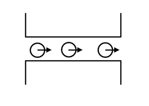
  $L_2-L_1=L$. The cylinder ends open into large reservoirs (figure 3). In § 4.1 the analysis of § 2 for the electric field in the narrow gap between a single sphere (centred at $(r,z)=(0,0)$) and the cylinder wall is combined with an estimate of the electric field far from the sphere, and it is straightforward to extend this analysis in order to estimate the electric field when $N$ well-spaced spheres are present. In § 4.2 we perform similar steps for the pressure field, and obtain a prediction for the electrophoretic velocity, which is compared against experimental results in § 4.3.

Figure 3. The liquid-filled cylinder has total length  $L=L_2-L_1$. The figure shows the case of one sphere ( $N=1$) at $z=0$, with two sections of liquid-filled pipe of length $L_2-a$ and $-L_1-a$, in which the electric field and pressure gradient are assumed uniform.
4.1. The electric field
A potential difference  $V$ is applied between the two liquid reservoirs at each end of the cylindrical tube, such that the electric field is $\boldsymbol E_0 =E_0\hat {\boldsymbol z}$ within the cylinder far from any sphere. In the absence of spheres and of any end effects, $E_0=V/L$. We model electrical end effects by the electric field around a circular hole in a membrane of zero thickness (Sherwood, Mao & Ghosal Reference Sherwood, Mao and Ghosal2014). This end effect is discussed in detail in the context of acoustic impedance by Brandão & Schnitzer (Reference Brandão and Schnitzer2020). In the absence of any sphere, but when end effects are included, the imposed electric field within the pipe is
 \begin{equation} E_0\approx\frac{V}{L+{\rm \pi} R/2}. \end{equation}
In § 2 we showed that the total drop in potential (2.14) across the particle is
 \begin{equation} [\phi]_{-\infty}^\infty={-}\frac{E_0R^2{\rm \pi} }{(2ah_0)^{1/2}}. \end{equation}
The electric field  $E_0$ away from the particle (i.e. in the liquid-filled portion of the cylinder, of length approximately $L-2a$) contributes a potential difference $E_0(L-2a)$, and end effects add a potential difference $E_0{\rm \pi} R/2$. The total potential drop between the two reservoirs is therefore
 \begin{equation} V\approx E_0\left[ \frac{{\rm \pi} R}{2}+(L-2a)+\frac{{\rm \pi} R^2}{(2ah_0)^{1/2}} \right]. \end{equation}
Analogous arguments predict that when there are  $N$ particles
 \begin{equation} V\approx E_0\left[\frac{{\rm \pi} R}{2}+(L-2Na)+\frac{N{\rm \pi} R^2}{(2ah_0)^{1/2}} \right]. \end{equation}
 We assume that  $L/R\approx L/a\gg 1$, which enables us to neglect terms in (4.4) that have been estimated, rather than rigorously derived. The electric field (4.4) away from any of the spheres therefore simplifies to
 \begin{equation} E_0\approx V\left[ L+\frac{N{\rm \pi} R^2}{(2ah_0)^{1/2}} \right]^{{-}1} =\frac{V}{L}\left[ 1+\frac{N{\rm \pi} R^2}{L(2ah_0)^{1/2}} \right]^{{-}1}.\end{equation}
The correction term on the right-hand side of (4.5) is  $O(\epsilon ^{-1/2}R/L)$, and as long as this is small we may expand (4.5) to obtain the electric field $E_0$ away from any of the spheres in the form
 \begin{equation} E_0 =\frac{V}{L}\left(1-\frac{N{\rm \pi} R^2}{L(2ah_0)^{1/2}} +\cdots\right).\end{equation}
 We see from (4.6) that one effect of increasing the number of spheres,  $N$, within the cylinder is to decrease the electric field $E_0$ away from any sphere if $V$ is held constant. This effect on its own would tend to reduce the electrophoretic velocity of the spheres to below that of a single sphere.
4.2. The pressure field
As in § 4.1 for the electric field, we first examine electrophoretic motion of a single sphere with centre at  $z=0$, and determine the pressure generated by this motion. The results will then be generalized to the case of $N$ spheres along the centreline. We assume that the ends of the cylinder open into liquid-filled half-spaces, both of which are at pressure $P_0$. The pressure at the right-hand end of the cylinder, $z=L_2$, is $P_2$, and that at the left end $z=L_1$ is $P_1$ (figure 3). The pressure losses due to a volumetric flow rate $Q_L$ into and out of the ends of the pipe are each approximated as $3Q_L\mu /(2R^3)$, based on flow through a hole of radius $R$ in a membrane of zero thickness (Happel & Brenner Reference Happel and Brenner1973). The (small) errors due to this approximation are discussed by Dagan, Weinbaum & Pfeffer (Reference Dagan, Weinbaum and Pfeffer1982).
We assume that the pressure  $p$ tends towards $P_{\infty }$ as we move away from the sphere into a region $z>a$ sufficiently far from the particle for the pressure gradient to be unaffected by the presence of the sphere. Similarly $p$ tends to $P_{-\infty }$ away from the sphere in $z<-a$, and in § 3.5 we obtained an estimate (3.58) for the pressure difference ${\rm \Delta} p=P_{\infty }-P_{-\infty }$ in terms of the (as yet unknown) electrophoretic velocity $U$ and any pressure driven volumetric flow rate $Q_L$.
Looking at the Poiseuille flow in the left- and right-hand parts of the liquid-filled pipe, the lengths of which we approximate as  $-L_1-a$ and $L_2-a$, and at the pressure losses due to entrance and exit effects at the ends of the cylinder, we find
 \begin{equation} Q_L=\frac{{\rm \pi} R^4(P_{\infty}-P_2)}{8\mu(L_2-a)} =\frac{{\rm \pi} R^4(P_1-P_{-\infty})}{8\mu({-}L_1-a)} =\frac{2R^3(P_0-P_1)}{3\mu}=\frac{2R^3(P_2-P_0)}{3\mu}.\end{equation}
Hence
 \begin{equation} \frac{8\mu Q_L}{{\rm \pi} R^4}[ L-2a] =P_1-P_2+{\rm \Delta} p, \end{equation}
and since the two reservoirs are at the same pressure  $P_0$,
 \begin{equation} \frac{3\mu Q_L}{R^3}=P_2-P_1, \end{equation}
so that
 \begin{equation} {\rm \Delta} p=\frac{8\mu Q_L}{{\rm \pi} R^4}\left[ L-2a+\frac{3{\rm \pi} R}{8}\right]. \end{equation}
If there are  $N$ spheres, an analysis including the pressure drop in each of the $N+1$ portions of the cylinder not containing a sphere leads to
 \begin{equation} N{\rm \Delta} p=\frac{8\mu Q_L}{{\rm \pi} R^4}\left[ L-2Na +\frac{3{\rm \pi} R}{8} \right].\end{equation}
As for the electric field, we now assume  $R\ll L$, so that (4.11) simplifies to
 \begin{equation} N{\rm \Delta} p=\frac{8\mu Q_LL}{{\rm \pi} R^4}.\end{equation}
We rewrite (4.12) in terms of the non-dimensional expansions for  $p$ (3.14c) and $Q_L$ (3.28):
 \begin{equation} Q_{L1}=\frac{N{\rm \pi} R^4{\rm \Delta} p_1}{8 a^3L\epsilon^{5/2}}.\end{equation}
We have ignored perturbations to the electroosmotically generated volume flow rate due to electroosmotic effects at the two ends of the cylinder. Such entrance and exit effects may be important when salt concentrations are low and surface conductivities large (Lee et al. Reference Lee, Joly, Siria, Biance, Fulcrand and Bocquet2012). However, we have assumed that Debye lengths are small and zeta potentials not too large, so that surface conductivity is negligible.
We use (4.13) in order to eliminate  $Q_L$ from the expression (3.58) for ${\rm \Delta} p_1$, leading to
 \begin{equation} {\rm \Delta} p_1\left[ \frac {1}{2^{1/2}{\rm \pi} }+ \frac{9 NR^4}{32 La^3\epsilon^{5/2}}\right] ={-}(\hat\zeta^{s}-\hat\zeta^{c})\frac{5}{4} +\frac{9 U_1R^2}{4a^2}.\end{equation}
We now reconsider the force balance (3.59) on our control volume, using (3.44), and find at  $O(\epsilon ^{-3/2})$
 \begin{equation} \frac{{\rm \pi} R^2}{a^2}{\rm \Delta} p_1={\rm \pi} R^2\frac{9U_1R^2/(4a^2)-5(\hat\zeta^{s}-\hat\zeta^{c})/4}{1/(\sqrt 2{\rm \pi} )+9NR^4/(32La^3\epsilon^{5/2})}=\frac{\sqrt 2{\rm \pi} ^2R}{2a}(\hat\zeta^{s}-\hat\zeta^{c}), \end{equation}
and hence
 \begin{equation} U_1=(\hat\zeta^{s}-\hat\zeta^{c})\frac{a^2}{R^2}\left[ \frac{7}{9}+\frac{R^3N\sqrt2{\rm \pi} }{16La^2\epsilon^{5/2}}\right]. \end{equation}
The non-dimensional electrophoretic velocity of the  $N$ spheres is therefore
 \begin{equation} U_0+\epsilon U_1+\cdots =\frac{(\hat\zeta^{s}-\hat\zeta^{c})}{2} \left[ 1+\frac{14\epsilon}{9}+\frac{R^3N\sqrt2{\rm \pi} }{8La^2\epsilon^{3/2}}\right].\end{equation}
Writing this in dimensional terms, and using (4.6) to express the electric field  $E_0$ in terms of the applied potential difference $V$
$V$
 \begin{equation} U=\frac{\epsilon_l(\zeta^{s}-\zeta^{c})}{2\mu}\frac{V}{L} \left(1-\frac{N{\rm \pi} R^2}{L(2ah_0)^{1/2}}\right) \left[ 1+\frac{14h_0}{9a}+\frac{R^3N\sqrt2{\rm \pi} }{8La^{1/2}h_0^{3/2}}\right]. \end{equation}
We see that the reduction in velocity due to the reduction in the electric field  $E_0$ (4.6) is $O(h_0/R)$ smaller than the increase in velocity due to the pressure-driven flow and may be neglected, leaving
 \begin{equation} U =\frac{\epsilon_l}{2\mu}(\zeta^{s}-\zeta^{c}) \frac{V}{L} \left\{ 1+\frac{14h_0}{9a}+\frac{NR^3\sqrt 2{\rm \pi} }{8La^{1/2}h_0^{3/2}}+\cdots \right\}.\end{equation}
This tends to our previous result (3.62) in the limit  $L\rightarrow \infty$. As might be expected, the rate of increase in electrophoretic velocity is largest when $h_0$ is small, so that leakage fluxes past the spheres are small. The increase becomes infinite in the limit $h_0\rightarrow 0$. However, we have assumed $h\gg \kappa ^{-1}$. Moreover, if liquid velocities and electric fields become too large within the narrow gap, the charge clouds will be deformed (Sherwood & Ghosal Reference Sherwood and Ghosal2018), and an analysis based solely on the Smoluchowski slip velocity (3.1) no longer suffices.
If, as earlier in (3.64), we replace  $\epsilon =h_0/a$ in (4.17) by $\delta =h_0/R$, the prediction (4.19) for the electrophoretic velocity becomes
 \begin{equation} U =\frac{\epsilon_l}{2\mu}(\zeta^{s}-\zeta^{c}) \frac{V}{L} \left\{1+\frac{14h_0}{9R}+\frac{NR^{9/2}\sqrt 2{\rm \pi}}{8La^{2}h_0^{3/2}}+\cdots \right\}.\end{equation}
4.3. Comparison with experiments
We now look at the experiments of Misiunas & Keyser (Reference Misiunas and Keyser2019), who used particles of diameter  $2a=505\ \textrm {nm}$ in a rectangular channel with side $2b=750\ \textrm {nm}$ and length $L=10^4\ \textrm {nm}$. We consider an effective cylinder radius $R=423\ \textrm {nm}$ such that ${\rm \pi} R^2=4b^2$, leading to estimates $h_0=R-a=171\ \textrm {nm}$, $L/R=23.6$, $h_0/R=0.4$, $\epsilon =h_0/a=0.68$, $a/R=0.6$, $\delta =h_0/R=0.4$. Misiunas & Keyser (Reference Misiunas and Keyser2019) do not state the Debye length in their experiments, but an electrolyte concentration of 2 mM KCl suggests $\kappa ^{-1}\approx 7\ \textrm {nm}$, so that $\kappa ^{-1}\ll h_0$. Similarly our assumption $R\ll L$ is satisfied. The gap width $h_0$ is sufficiently large that we see from figure 2 that our predicted velocity $U$ (3.62) in an infinite cylinder is poor, but the transformed expression (3.64) remains good, and we adopt this here. Our predicted velocity, using (4.19) for the increase in velocity due to the finite length of the cylinder, is therefore
 \begin{equation} U(N)=\frac{\epsilon_lV}{\mu L}(\zeta^{s}-\zeta^{c}) \left\{ \frac{1}{2}+\frac{7\delta}{9} +\frac{NR^3\sqrt 2{\rm \pi} }{16La^{1/2}h_0^{3/2}} \right\}=0.93\frac{\epsilon_lV}{\mu L}(\zeta^{s}-\zeta^{c}) [1+0.07(N-1)].\end{equation}
If instead we use (4.20), our prediction becomes
 \begin{equation} U=0.94\frac{\epsilon_lV}{\mu L}(\zeta^{s}-\zeta^{c}) [ 1+0.13(N-1)].\end{equation}
 The experiments of Misiunas & Keyser (Reference Misiunas and Keyser2019) found that the electrophoretic velocity of  $N$ spheres, $U(N)\approx U(1)[1+0.09(N-1)]$, increases linearly with $N$ only slightly faster than predicted by (4.21) or less than predicted by (4.22). This agreement between theory and experiment is much better than one might expect, given the square cross-section of the experimental flow channel and the only moderately small experimental value of $h_0/a$.
The theoretical prediction of the dependence of the electrophoretic velocity on the number of particles  $N$ in the cylinder, obtained above ((4.20) and (4.19)) complements the experimental and numerical results of Misiunas & Keyser (Reference Misiunas and Keyser2019). Our analysis requires the particles to be spherical, and only slightly smaller in diameter than the circular cylinder along which they move. The Debye length must be thin compared with the minimum gap width between the cylinder wall and the particle. The zeta potentials on the surfaces of the particles and cylinder are assumed to be sufficiently small so that surface conductivity can be neglected: this constraint is usually satisfied if, as here, Debye lengths are small. We have assumed that the particles lie along the axis of the cylinder: the effect of radial position of the particle has been studied (for the case of a single particle in an infinite cylinder) by Yariv & Brenner (Reference Yariv and Brenner2003). The cylinder length $L$ is assumed to be long compared with the particle radius $a$, so that the pressure-driven flow is dominated by Poiseuille flow in the particle-free portions of the cylinder, and the particle separation is assumed to be large compared with the cylinder diameter $2R$, so that hydrodynamic interactions other than those due to the volumetric flow of liquid are negligible.
Electrophoresis experiments in which the particle diameter is only slightly less than that of the liquid-filled cylinder are perhaps rare, since the particle might be attracted to the cylinder wall if the two surfaces have opposite sign or (at close range) even if they have different fixed charge densities of the same sign (Israelachvili Reference Israelachvili2011). Entry into such a cylinder may lead to clogging, and particles accumulated outside (but did not clog) the channel entrance in the experiments of Misiunas & Keyser (Reference Misiunas and Keyser2019). However, our predictions (4.21) and (4.22) appear to be useful even when the gap is as large as  $h_0/R=0.4$, and may therefore serve to help design experiments in which the cylinder length $L$ is sufficiently long for bulk volumetric flow and end effects to be negligible.
Acknowledgements
We thank Professor E. Yariv (Technion) for helpful suggestions. J.D.S. thanks the Department of Applied Mathematics and Theoretical Physics, University of Cambridge, for virtual hospitality.
Funding
This research received no specific grant from any funding agency, commercial or not-for-profit sectors.
Declaration of interest
The authors report no conflict of interest.


 Open access