4.1. Instantaneous flow visualisation

Observing the instantaneous flow reveals the emergence of numerous spatial scales as $Re_\tau$ increases. Figure 1 shows streamwise velocity $u_z$ contours in a cross-stream plane and on a near-wall cylindrical shell at $y^+ \approx 15$ ($y^+=(R-r)^+$), similar to Pirozzoli et al. (Reference Pirozzoli, Romero, Fatica, Verzicco and Orlandi2021) but with a much longer axial extent.

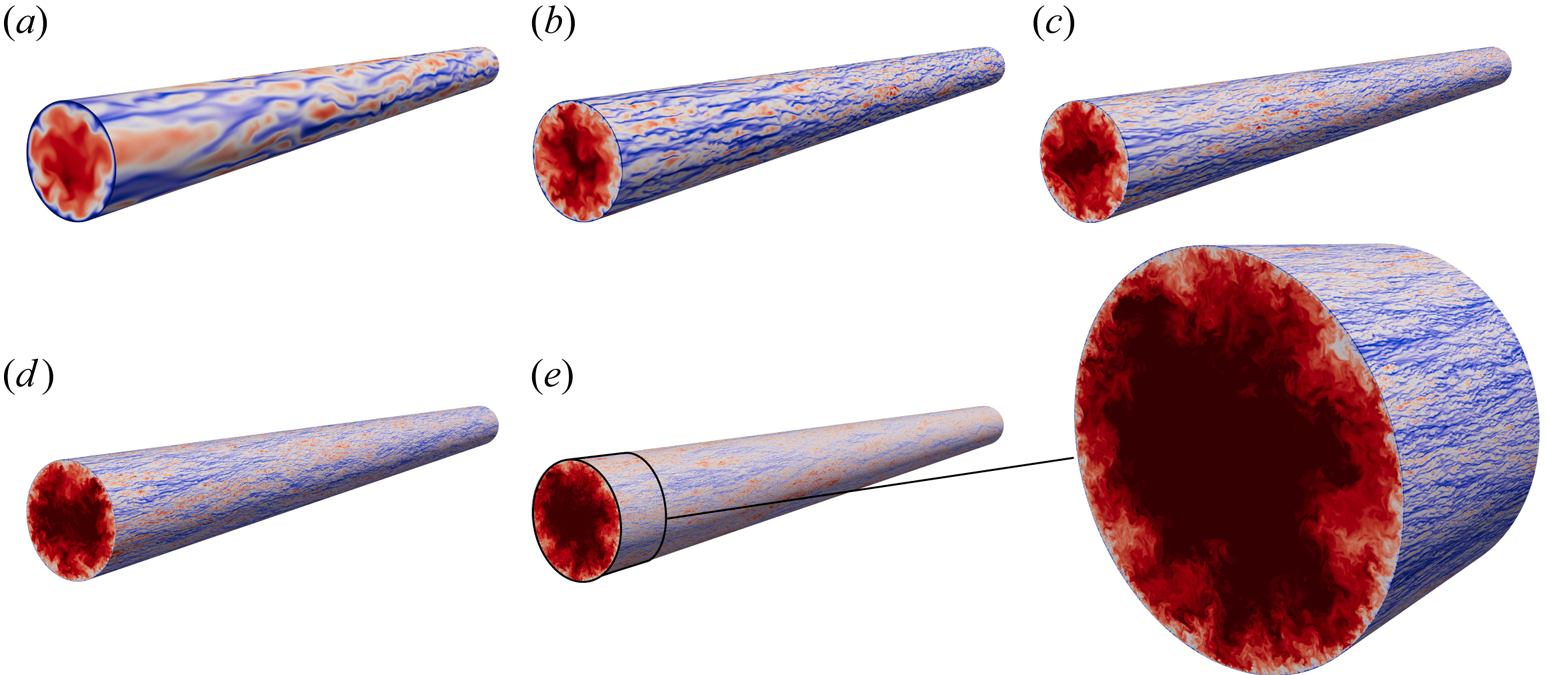
Figure 1.

Instantaneous streamwise velocity contours ($u_z$) with low- and high-speed velocity streaks in blue and red, respectively. Panels (a–e) show a cross-stream plane and a near-wall cylindrical shell ($y^+ \approx 15$) at $Re_\tau =180, 550, 1000, 2000$ and $5200$.

In the cross-stream planes the flow consistently exhibits a limited number of bulges distributed azimuthally. These low azimuthal wavenumber patterns correspond to regions where high-speed fluid enters from the pipe's core while low-speed fluid is ejected from the wall. As discussed below, their resemblance to the POD modes is quite striking, as previously reported at lower Reynolds numbers by Hellström, Ganapathisubramani & Smits (Reference Hellström, Ganapathisubramani and Smits2015). In all cases, large scales dominate in the central region of the pipe. Figure 1 shows, among the multitude of small streaks, elongated regions of low and high velocity, in blue and red, respectively. These streaks have an average spacing of $(R\theta )^+ \approx 100$ and are elongated in $z$. In the near-wall cylindrical shell at $y^+ \approx 15$, streaks are observed with an arrangement visibly connected to the cross-stream pattern, as seen at $Re_\tau =180$ in figure 1(a). As $Re_\tau$ increases, the scale separation gets larger, the near-wall streaks scale in wall units, and the centre modes scaling in integral scales become more and more distinct.

Decomposing the flow according to the KL expansion, we aim to understand the spatial (temporal) correlation between instantaneous structures. The near-wall dynamics of streaks have been extensively discussed in the past and the influence of the Reynolds number on the autonomous wall cycle is limited, if not entirely negligible (Jiménez & Pinelli Reference Jiménez and Pinelli1999). Therefore, for the remainder of the paper, our focus is on the larger scales in the outer layer, rather than the buffer layer and viscous sublayer.

4.2. The POD modes hierarchy

The 10 most energetic modes at the five Reynolds numbers considered are listed in table 2. For each wavenumber pair ($\kappa _\theta$, $\kappa _z$), the corresponding quantum index and the fraction of the fluctuating energy $f=\lambda _{(q,p)}/k$ are reported. The energy fraction is computed relative to the total fluctuating energy. Note that the mean flow is not subtracted in advance, thus, it corresponds to the zeroth POD mode, and it is not reported in table 2.

Table 2.

The 10 most energetic POD modes at $Re_\tau =180, 550, 1000, 2000$ and $5200$: the azimuthal and streamwise wavenumber ($\kappa _\theta$, $\kappa _z$), the quantum index ($q$) and the fraction of the total fluctuating kinetic energy ($\,f=\lambda _{(q,p)}/k$, with $p=$($\kappa _\theta$, $\kappa _z$)).

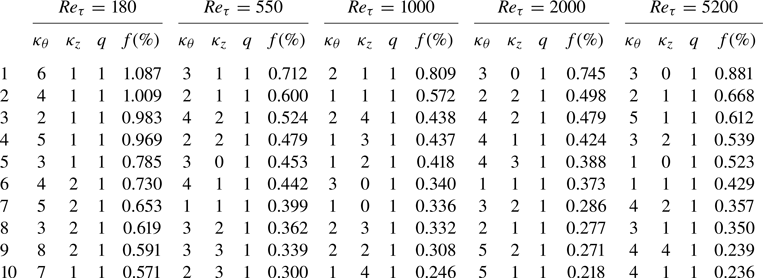
At the lowest Reynolds number ($Re_\tau =180$), the most energetic modes are characterised by a large number of streaks in the cross-stream planes, with the azimuthal wavenumber varying from 2 to 8. The POD mode 1 corresponds to six pairs of streamwise streaks that qualitatively resemble the evenly distributed low-speed streaks in figure 2(a). Their maximum magnitude is located at $y^+ \approx 20$, with an azimuthal separation of $\Delta R\theta ^+ \approx 85$ and an axial wavelength of $\Delta z^+ \approx 1000$. The POD mode 1 makes a substantial contribution, approximately 1.1 %, to the total kinetic energy. Note that a single POD mode does not represent a dynamic flow feature, but it does provide an indication of the energetic level of such structures. Therefore, we have examined the evolution of the POD mode 1 as $Re_\tau$ increases to understand how the mode and its energetic contribution vary. Since only the first 32 modes in the axial and azimuthal directions are retained in the POD calculation, we can identify the equivalent mode at $Re_\tau =550$ and $1000$ only. At higher Reynolds numbers, the mode exhibits wavenumbers beyond 32. As one would expect, the mode shape is maintained, i.e. the mode resembles near-wall streaks, but the energy contribution drops significantly; see figure 2(b). This decrease occurs because larger structures in the outer layer contain the majority of the energy. The POD mode 342 ($\kappa _\theta =18$, $\kappa _z=3$) at $Re_\tau =550$ and the POD mode $2382$ ($\kappa _\theta =32$, $\kappa _z=6$) at $Re_\tau =1000$, contribute only 0.0259 % and 0.0017 % to the total kinetic energy, respectively. The energy is spread across a wider range of scales with the larger scales containing a higher portion of the energy. As stated earlier, the energy contributions of multiple POD modes that describe a single dynamical feature, such as the streaks, should be combined.

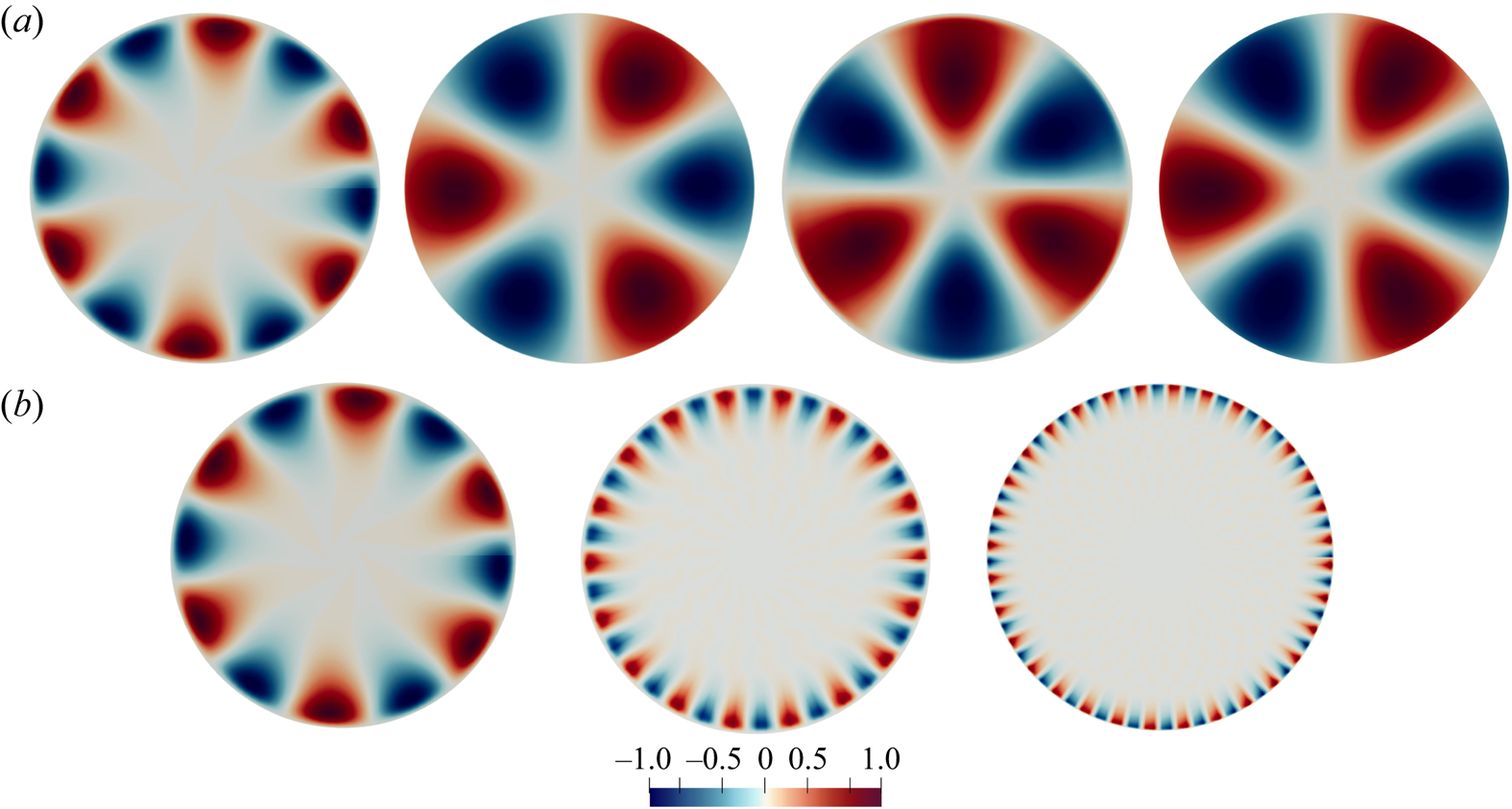
Figure 2.

(a) From left to right, cross-stream planes of the streamwise velocity of the most energetic POD modes $\hat {\varPhi }_{(q=1,p)}(r)$ (normalised by their maximum) at $Re_\tau =180, 550, 2000, 5200$. (b) Scaling of the most energetic POD mode at $Re_\tau =180$, i.e. near-wall streaks, at higher Reynolds numbers $Re_\tau =550$ and $1000$.

When the Reynolds number increases, the energy contribution of the top-ranked modes, as the POD mode 1, gradually diminishes. Notably, starting from $Re_\tau =550$, a mode with $\kappa _z=0$ appears in table 2. This becomes the dominant mode at the highest Reynolds numbers, contributing 35 % more energy than the POD mode 2. Observe that an eddy with $\kappa _z=0$ represents a structure with a wavelength longer than the entire pipe, despite the considerable length of the current set-up ($L_z=10 {\rm \pi}R$). Modes with $\kappa _z=0$ were previously classified by Duggleby et al. (Reference Duggleby, Ball, Paul and Fischer2007) as non-propagating modes, and further categorised into shear ($\kappa _\theta =0$) and roll ($\kappa _\theta \neq 0$) modes. The contribution of the non-propagating modes to the total fluctuating energy increases with the Reynolds number. In particular, these modes constitute approximately 1.6 % and 2.1 % of $k$ at $Re_\tau =2000$ and $5200$, respectively. The shear modes contribute 0.38 % and 0.54 % at $Re_\tau =2000$ and 5200, respectively, while the roll modes contribute more: 1.22 % and 1.56 % at $Re_\tau =2000$ and 5200, respectively.

In general, a distinct pattern emerges: with increasing Reynolds numbers, structures that maintain spatial correlation over more than $3R$ become more energetically significant. These structures have been referred to as VLSMs in turbulent pipe flows (Adrian et al. Reference Adrian, Meinhart and Tomkins2000). Using an array of hot wires and operating under Taylor's hypothesis, Monty et al. (Reference Monty, Stewart, Williams and Chong2007) also documented the existence of long meandering features in both pipe and channel flows. These features qualitatively resemble those observed in boundary layers, with lengths of the order of $O(20 \delta )$ (Hutchins & Marusic Reference Hutchins and Marusic2007). Based on the above definition of the VLSM ($\lambda _z > 3R$), the VLSM contribution to the total $k$ is seen to increase with Reynolds number, particularly reaching around 14 % and 16 % at $Re_\tau =2000$ and 5200, respectively.

The VLSM with $\kappa _\theta =3$ and $\kappa _z=0$ appears as most energetic at $Re_\tau =2000$ and $5200$ and consistently ranks among the top six from $Re_\tau =550$ to $5200$. It is worth noting that this mode ($\kappa _\theta =3$, $\kappa _z=0$) has already been reported previously. Bailey & Smits (Reference Bailey and Smits2010), despite not observing a clear distinction between VLSMs and LSMs, reported that a VLSM tends to be concentrated within the lower azimuthal modes, typically around $\kappa _\theta =3$. This observation aligns with the large transverse scales reported in the spectrally filtered results, also discussed in Bailey & Smits (Reference Bailey and Smits2010). In contrast, the LSM appears to be distributed across a broader range of azimuthal scales, hence, no dominant transverse scale and spanning a wide range of streamwise and transverse scales. Our results, covering a wider range of Reynolds numbers and higher values, support their observations, as illustrated by the mode hierarchy in table 2. This finding is also in line with other studies that consistently identify modes around ($\kappa _\theta =3$, $\kappa _z=0$) as the energetically dominant (Baltzer et al. Reference Baltzer, Adrian and Wu2013; Hellström et al. Reference Hellström, Marusic and Smits2016). Furthermore, there may be a noteworthy connection with transitional pipe flow. Faisst & Eckhardt (Reference Faisst and Eckhardt2003) and Eckhardt et al. (Reference Eckhardt, Schneider, Hof and Westrweel2007) predicted that nonlinear travelling wave instabilities exhibiting threefold azimuthal symmetry are the first to appear with increasing Reynolds numbers, marking the transition to turbulence in pipe flow. Experimental observations by Hof et al. (Reference Hof, van Doorne, Westerweel, Nieuwstadt, Faisst, Eckhardt, Wedin, Kerswell and Waleffe2004) have also identified states with up to sixfold symmetry. Their findings align with the range of the azimuthal modes observed in the VLSM wavenumbers within turbulent flows. This suggests that the VLSMs stem from the persistence of unstable travelling waves that originate during the transition phase and continue into the turbulent flow regime. However, as discussed by Bailey & Smits (Reference Bailey and Smits2010), some inconsistencies need to be considered. Firstly, the formation mechanism of these travelling waves in transitional flows is inherently unstable, making it challenging for these modes to persist in turbulent flows where the mean shear is significantly different. Secondly, the wavelengths observed by Faisst & Eckhardt (Reference Faisst and Eckhardt2003) are much shorter than those of the VLSM. This latter difference could be explained by the fact that the wavelength of the instability depends on the Reynolds number and azimuthal mode, generally increasing with higher Reynolds numbers and decreasing with higher azimuthal modes.

From our perspective, the persistence of the roll modes with $\kappa _\theta =3$ at different Reynolds number regimes (and in many different works) is unlikely to be a mere coincidence. A possible explanation could be that these modes represent exact solutions in the state space of parallel shear flows (Pringle & Kerswell Reference Pringle and Kerswell2007; Duguet, Willis & Kerswell Reference Duguet, Willis and Kerswell2008). Although further studies are required in this direction, the consistency between VLSMs and the travelling wave instability with $\kappa _\theta \approx 3$ is important and further corroborated by the present results at high Reynolds numbers.

4.3. Spatial classification

The POD analysis has proven valuable by providing insights into energy variations across the inhomogeneous wall-normal direction (Hellström et al. Reference Hellström, Marusic and Smits2016). In the current formulation, the KL decomposition exploits the two homogeneous directions, defining one-dimensional modes (varying in the radial direction) for a given triplet $\boldsymbol {k} = (q,\kappa _{\theta },\kappa _z) = (q,p)$. For each mode, we only consider the dominant peak, specifically using $q=1$ for each triplet, which represents the most energetic structure within a wavenumber pair $p$. It is important to note that the below classification holds when all pairs are included, i.e. $q=1,\ldots,\tilde {N}$ for each triple $\boldsymbol {k}=(q,p)$ (Massaro et al. Reference Massaro, Yao, Rezaeiravesh, Schlatter and Hussain2024).

A MATLAB code is used to extract the spatial characteristics of the POD modes, as shown in figure 3. Each structure is characterised by the peak height ($h$), peak location ($y_p$) and mode thickness ($l_y$), all normalised by $R$. The size $l_y$ represents the radial extension $l_y=y_c-y_w$. The coordinates $y_w$ and $y_c$ are the radial locations where the peak halves towards the wall ($y=R-r=0$) and towards the centre ($y=1$), respectively. The positions $y_w$ and $y_c$ mark the structure's start and end points, offering insight into the degree of asymmetry, as the peak is not necessarily symmetric. The depiction of the coordinates $y_w$ and $y_c$ as the positions where the peak halves occur is reasonable and customary, but to some extent arbitrary. Alternative definitions for assessing the size of the structure would yield a similar classification, albeit leading to a potentially unrealistic estimation of the radial thickness. The classification is conducted in spectral space for the streamwise velocity component $u_z$. The solid black line in figure 3 illustrates $|u_z|$ and the spatial characteristics of the POD mode for a generic $\boldsymbol {k}=(q=1,p)$. Similar results are obtained by classifying in physical space and then averaging in the streamwise and azimuthal directions.

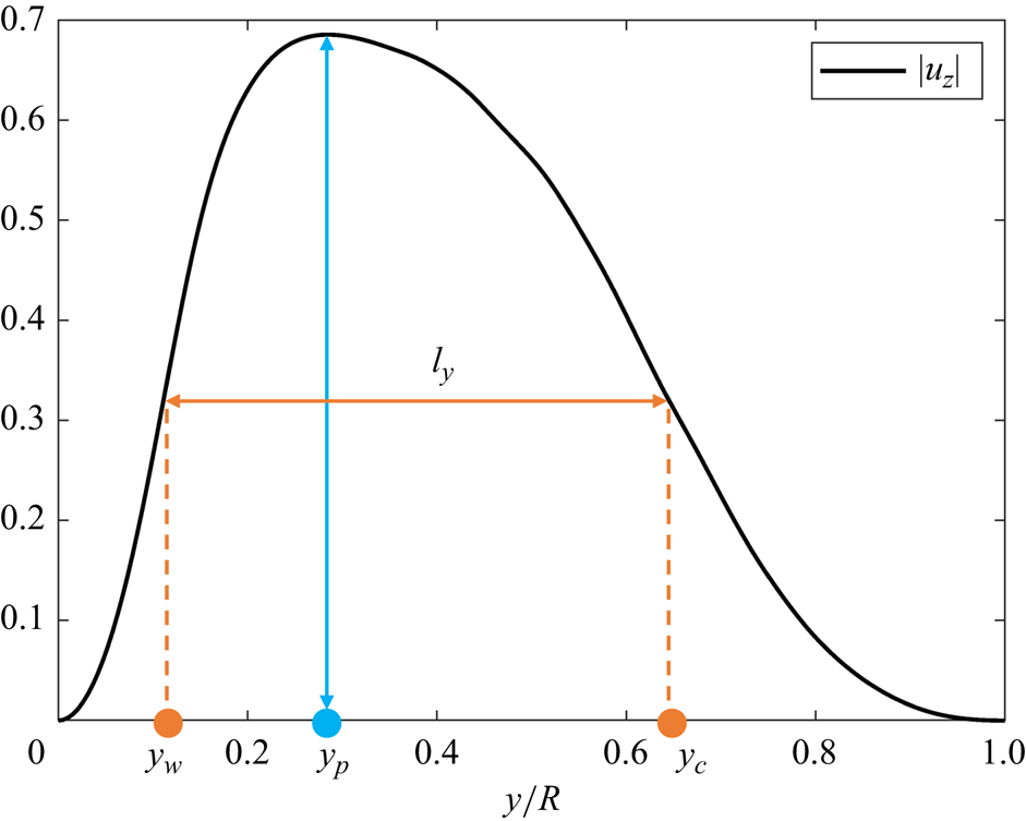
Figure 3.

Illustration of the spatial characteristics of a generic POD mode. The modulus of the (complex) streamwise velocity is shown together with the height of the largest peak $h$ (blue), the wall-normal position of the peak $y_p$ and the thickness of the mode $l_y$ (orange). The wall distances at half-amplitude, $y_w$ and $y_c$, indicate the beginning and the end of the structure, respectively. The wall and the pipe centre are located at $y=0$ and $y=R$, respectively. All the lengths are normalised by $R$.

4.3.1. Voronoi tessellation

The KL decomposition produces spatially orthogonal modes whose energetic contributions add up to the total fluctuating kinetic energy. Therefore, when examining the energy distribution in the radial direction, the density of POD modes at a particular location is essential, as their contributions are cumulative. An example at $Re_\tau =2000$ is displayed in figure 4. In panel (a) each point represents the energy contribution of a mode with size $l_y$ and the peak at radial position $y_p$. The intensity of the colour (over the blue-to-red range) indicates the mode's contribution to the total fluctuating energy. In panel (b) the contour plot of scattered points reveals a region with high energy between $0.12< y_p/R<0.5$ for $l_y/R > 0.45$ (upper vertex of the triangular contour plot). However, this plot represents the average energetic intensity and does not consider the density of the POD modes. Neglecting this aspect can lead to misleading results. For instance, a cluster of points at a specific $y$ location may contribute more to the total energy than a single point with high energy at the same location. This issue has been highlighted by Massaro et al. (Reference Massaro, Yao, Rezaeiravesh, Schlatter and Hussain2024). Thus, the density of points ($\rho$) should be considered. When we weigh the energy contribution, it significantly alters the shape of the contour plot, as shown in figure 4(c). The radial classification based on energy reveals the emergence of two branches, although they are not fully separated at this $Re_\tau$. These branches are classified and analysed in detail in the rest of this paper. Note that the contour plot undergoes substantial changes due to the consideration of the POD mode density. To accurately estimate the density $\rho$ for each point, a Voronoi diagram is utilised.

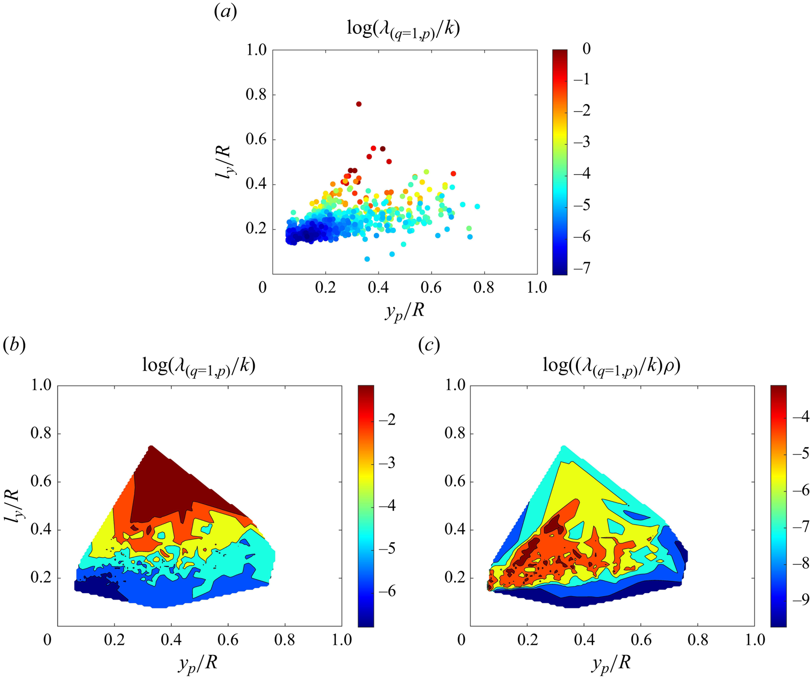
Figure 4.

(a) Scatter plot of the points corresponding to the radial size of the POD mode ($l_y$) at the wall-normal location of the peak ($y_p$) at $Re_\tau =2000$. The colour of the point indicates the energy content: the more intense the colour (in the blue–red scale), the more energetic the content is. (b) Contours of the energy in the scatter plot in (a). (c) Contours of the energy in the scatter plot in (a) weighted by the density estimated through the Voronoi tessellation.

Given a discrete set of points {$x_j, y_j$} for $j=1,\ldots, N_{TOT}$, the Voronoi diagram decomposes the space around each point ($x_j, y_j$) into a region of influence $\varOmega _j$, which ensures that any arbitrary point within $\varOmega _j$ is closer to point $j$ than to any other point. The Voronoi region $\varOmega _j$, with an area $A_j$, is referred to as the Voronoi region, and the collection of all these Voronoi regions forms the Voronoi diagram. A MATLAB algorithm was implemented to account for the external boundaries, where an infinite area of interest was generated. Further details can be found in Massaro et al. (Reference Massaro, Yao, Rezaeiravesh, Schlatter and Hussain2024), and an example is given in the supplementary material available at https://doi.org/10.1017/jfm.2024.776. The code defines an area ($A_j$) for each point, and the inverse of this area provides the density ($\rho _j$), representing the two-dimensional concentration of points. The Voronoi diagram, originally employed in fluid mechanics to describe the spatial structure of dispersed phases (Monchaux, Bourgoin & Cartellier Reference Monchaux, Bourgoin and Cartellier2010; García-Villalba, Kidanemariam & Uhlmann Reference García-Villalba, Kidanemariam and Uhlmann2012), is now utilised to represent the spatial energy distribution of the POD modes.

4.4. Attached and detached eddies

The Voronoi-based contour plot effectively quantifies the energy, more precisely, the logarithm of the energy contribution weighted by its density. As the Reynolds number increases, a clear trend emerges, and two different classes of POD modes emerge. We begin by providing a comprehensive description of the spatial properties of these modes and how the Reynolds number affects the size of the most energetic structures (figure 5). Henceforth, the energy contribution, i.e. the ratio of the eigenvalue obtained by the KL decomposition $\lambda _{q,p}$ to the total kinetic energy $k$, is weighted by the Voronoi density $\rho$ to account for the density of points in a region of the ($l_y/R$, $y_p/R$) space. A logarithmic scale is used for $(\lambda _{q,p}/k)\rho$. Note that the plots depicted in figure 5 do not capture energy information near the wall ($y=0$). This occurs as our analysis focuses specifically on LSMs, considering only the first 32 azimuthal and streamwise wavenumbers. Additionally, the classification of space is based on the location of the largest peak ($y_p/R=0$), which accurately represents the near-wall location only in an idealised scenario, as depicted in figure 3. However, the shapes of POD modes are more complex and asymmetric. These factors contribute to the lack of populated regions near the wall. It is important to keep these considerations in mind to avoid misinterpretation, as no near-wall filtering or shifting was applied.

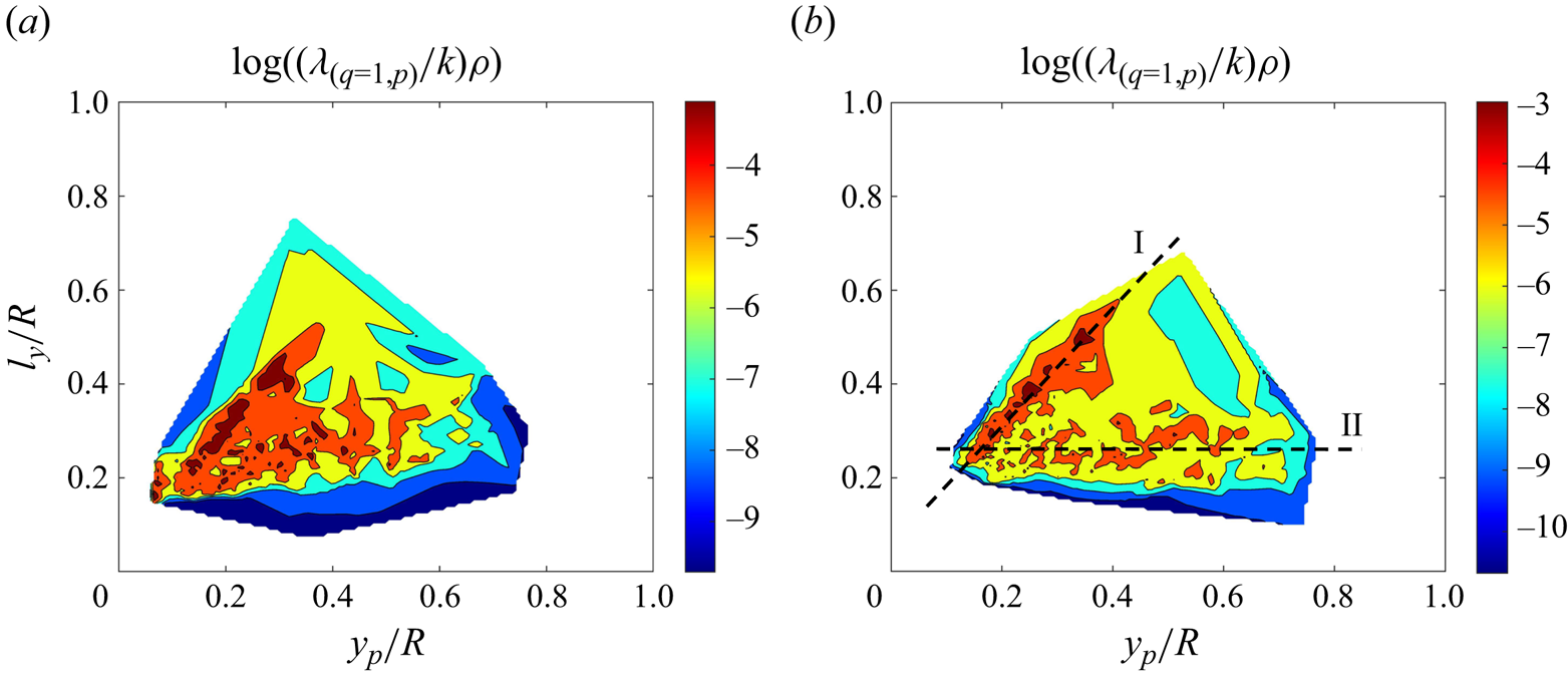
Figure 5.

Density-weighted energy contour of the scattered points {$y_p$, $l_y$}: $y_p$ is the radial location of the largest peak and $l_y$ is a measure of the structure's size. Plots (a,b) refer to $Re_\tau =2000$ and $5200$, respectively.

In figure 5 a specific $y_p/R$ point corresponds to the radial location of the largest peak of a structure that extends radially (not symmetrically) with a thickness denoted as $l_y$. At the lowest Reynolds numbers, the energy is concentrated in relatively small structures near the wall (Massaro et al. Reference Massaro, Yao, Rezaeiravesh, Schlatter and Hussain2024). Omitting the discussion of the results at the intermediate $Re_\tau =1000$ (which aligns with those at $Re_\tau =2000$), we find that at $Re_\tau =2000$, the energy is distributed across structures of varying sizes. The peak is located within a broad range of radial positions, specifically between $0.1R$ and $0.6R$. Among the most energetic structures, some exhibit peak positions beyond $0.5R$, near the centre of the pipe. In particular, the contour plot in (a) shows two distinct high-energy branches: the first is steep and extends up to $y/R \approx 0.4$ and the second reaches up to $y/R \approx 0.6$, but with a much lower slope. The distinction between these two classes of modes becomes even more obvious at $Re_\tau =5200$, where the two branches are definitely set apart; see figure 5(b). The first family represents a highly energetic class of POD modes, with their size linearly correlated to the wall-normal distance of their peak, denoted as $y_p$. The inclined dashed line (class I) exhibits a slope of $l_y \sim 1.29 y/R$ and $l_y \sim 1.20 y/R$ at $Re_\tau =2000$ and $5200$, respectively. The horizontal line represents another class of structures (class II) where the size remains nearly constant as the peak moves toward the centre of the pipe. The approximate values are $l_y \approx 0.25R$ at $Re_\tau =2000$ and $l_y \approx 0.26R$ at $Re_\tau =5200$, respectively.

However, the structure's size alone does not provide the complete picture. We also need to account for the degree of asymmetry. To this end, we calculate density-weighted contour plots for the starting ($y_w$) and ending ($y_c$) locations of the modes. Indeed, the energy distribution of the starting and ending points of the POD modes supports the classification into two distinct classes. At the two highest Reynolds numbers in the left panels of figure 6(a,b), two distinct branches are observed for $y_w$, which represents the wall-normal location of the beginning of the structures. The left panels show that the beginning of the detached eddies scales with $y$ as these structures detach from the wall. The scaling relationship is $y_w \sim 0.836 y/R$ at $Re_\tau =2000$ and $y_w \sim 0.938 y/R$ at $Re_\tau =5200$. Additionally, the horizontal energetic branch near $y_w \approx 0$ represents modes where the beginning is ‘attached’ to the wall, meaning that $y_w$ is constant over a range of $y_p$. As expected, the ending of the structures scales for both types of eddies, with linear trends of $y_c \sim 1.03 y/R$ for both Reynolds numbers.

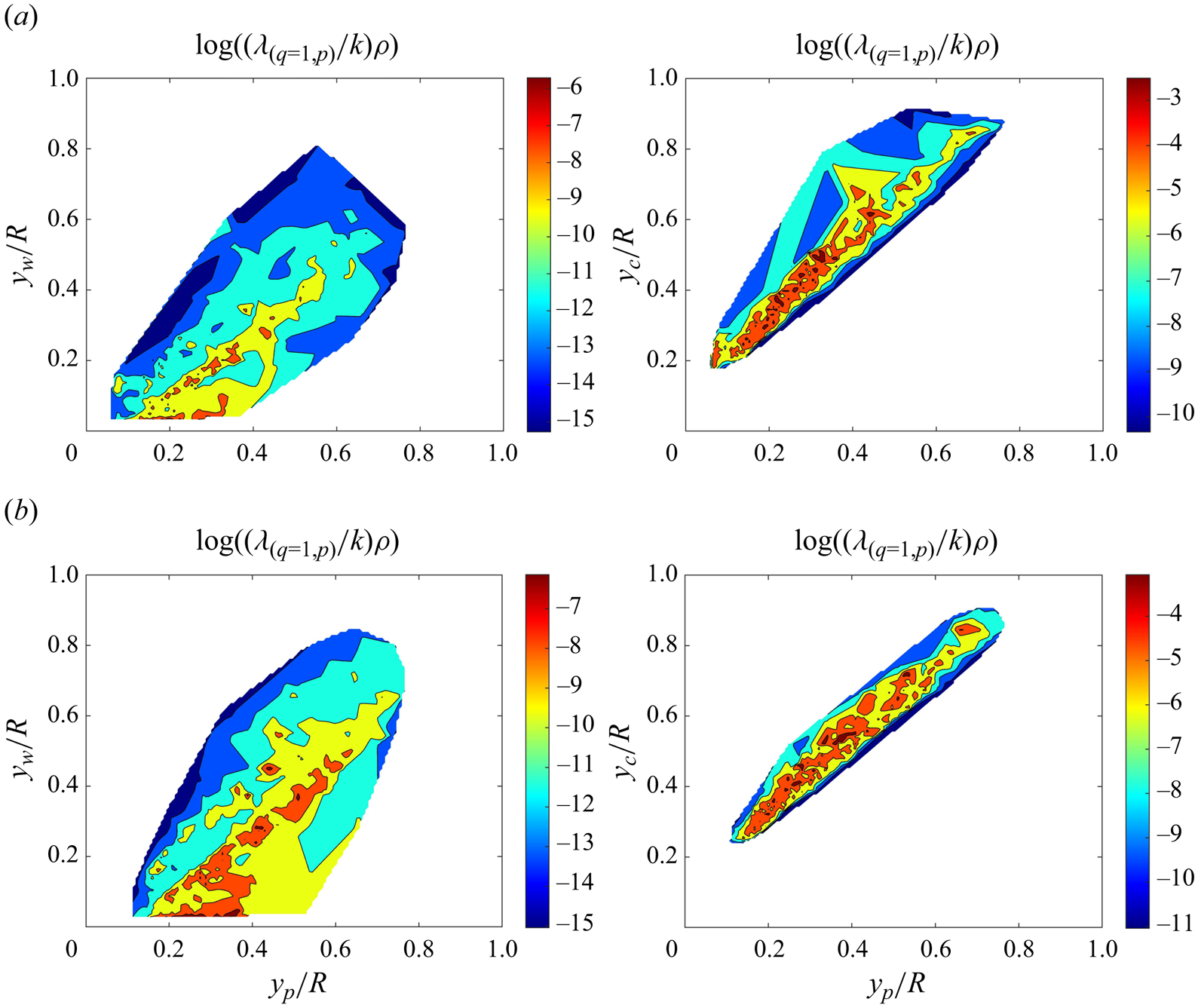
Figure 6.

Density-weighted energy contour of the scatter points (left) {$y_p$, $y_w$} and (right) {$y_p$, $y_c$}: $y_p$ is the radial location of the highest peak, $y_w$ and $y_c$ are the wall-normal distances indicating the beginning and the end of the structure, respectively. Plots (a,b) refer to $Re_\tau =2000$ and $Re_\tau =5200$, respectively.

The sets of points in the two branches are extracted based on the high-energy content and linearly fitted in the least squares sense. The resulting classes are indeed distinct in terms of the axial and azimuthal wavenumbers. At both $Re_\tau =2000$ and $5200$, class I (attached) and class II (detached) include only POD modes with $\kappa _\theta > \kappa _z$ and $\kappa _\theta < \kappa _z$, respectively. According to the previous classification by Duggleby et al. (Reference Duggleby, Ball, Paul and Fischer2007), these correspond to the wall and lift propagating modes, respectively, i.e. structures that turn azimuthally more than they lift axially ($\kappa _\theta > \kappa _z$) and that lift axially more than turning azimuthally ($\kappa _\theta < \kappa _z$). All the three highest Reynolds numbers depict these two classes, but, at $Re_\tau =5200$, in particular, they are clearly distinct. Figure 7 shows the modes that belong to class I and class II with blue and black lines, respectively. As observed above, class I consists of eddies whose size scales linearly with the wall-normal distance, whereas the size remains constant for class II. Figure 7(a) is crucial, as it concisely illustrates the core distinction between wall-attached (blue lines) and detached (black lines) eddies. This illustration makes the definition of the term ‘attached’ evident, reflecting the model outlined in Perry & Chong (Reference Perry and Chong1982). At a low Reynolds number the classification by Duggleby et al. (Reference Duggleby, Ball, Paul and Fischer2007) indicates a comparable energy content between the wall and lift modes, i.e. classes I and II, respectively. At $Re_\tau =5200$, the energy contained in the attached eddies is around 2 times larger than the energy in the detached eddies. This finding is of particular interest, especially in the context of the attached eddy model as discussed below.

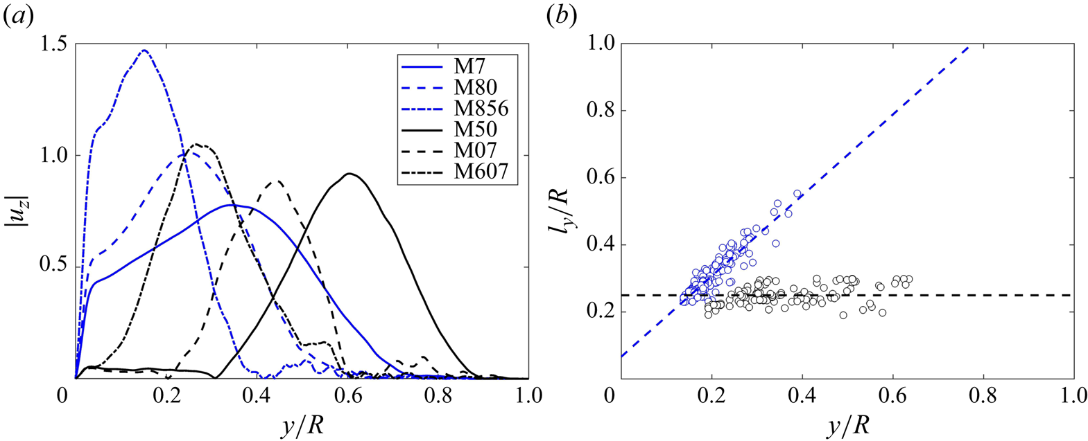
Figure 7.

(a) Modulus of the (complex) streamwise velocity of the POD modes belonging to the inclined (blue) and horizontal (black) branches. The legend indicates the POD mode number according to the global energy-based ordering. (b) The points belonging to the two red branches in figure 5 are extracted according to their energy level. As shown in (a), these correspond to attached and detached eddies, respectively. The dashed lines are obtained via linear regression in the least squares sense for the two sets of points, separately. Only data at $Re_\tau =5200$ are considered in (a,b).

As previously outlined, the size of the attached structures linearly scales with the wall-normal distance: $l_y \sim 1.29 y/R$ and $l_y \sim 1.20 y/R$ at $Re_\tau =2000$ and $Re_\tau =5200$, respectively. The result is consistent with the attached eddy model (Townsend Reference Townsend1976; Perry & Chong Reference Perry and Chong1982) as well as the previous findings (Hu et al. Reference Hu, Yang and Zheng2020). As $Re_\tau$ increases, a trend is also observed, with the slope decreasing from 1.42 ($Re_\tau =1000$) to 1.20 ($Re_\tau =5200$). However, it is important to note that studying a simplified one-dimensional representation of the statistically coherent structures emerging from the KL decomposition has its limitations. For example, the behaviour of $\lambda _z$ and $\lambda _{R\theta }$ as functions of $y$ cannot be investigated, in contrast to other studies (Hwang Reference Hwang2015; Deshpande et al. Reference Deshpande, de Silva, Lee, Monty and Marusic2021).

Eventually, the degree of asymmetry is also reported in figure 8 at $Re_\tau =2000$ and $5200$, respectively. The asymmetry of the mode is measured with respect to the radial location of the largest peak ($y_p$). The distance between where the structure begins ($y_w$) and the largest peak ($y_p$), and the distance between where the structure ends ($y_c$) and the largest peak ($y_p$) are used to estimate the asymmetry of the mode: $d_a=\log (|y_c-y_p|/|y_w-y_p|)$. For $d_a=0$, the structure is perfectly symmetric. In both cases, most of the modes are symmetric. A few structures with a remarkably non-symmetric behaviour appear for $d_a>2$ towards the centre of the pipe. These outliers are more numerous at higher Reynolds numbers. However, overall, the increase in the Reynolds number indicates a rise in the symmetry of the POD modes, with 64 % and 76 % of the modes falling within the range $|d_a|<0.4$ at $Re_\tau =2000$ and $5200$, respectively.

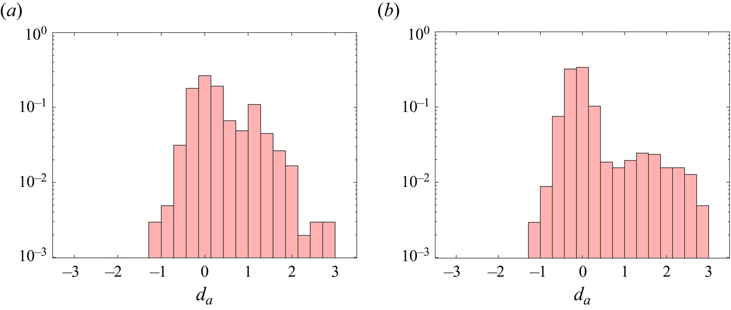
Figure 8.

Histograms of the degree of asymmetry ($d_a$) are reported (with a constant unitary area for each diagram). Panels (a,b) refer to $Re_\tau =2000$ and $5200$, respectively.

4.5. Modal self-similarity

The POD modes in the azimuthal and streamwise directions are Fourier harmonics and, therefore, inherently self-similar. On the other hand, the modes in the radial direction are data driven, and their shape function is not known a priori. Following Hellström et al. (Reference Hellström, Marusic and Smits2016), we explore the self-similarity to examine the presence of a universal length scale for the attached and detached eddies. In this context, we specifically focus on the self-similarity of the modal peak location.

The azimuthal and radial length scales of the eddies are estimated as follows. For any POD mode $\hat {\varPhi }_{(q=1,p)}(r)$, similar to the approach used in Hellström et al. (Reference Hellström, Marusic and Smits2016), we estimate the azimuthal wavelength as $\lambda _\theta = 2 {\rm \pi}(R-y_p)/\kappa _\theta$, where $(R-y_p)$ represents the radial location of the mode maximum. For the radial size, we employ the wall-normal location of the peak. In figure 9 we present the wall-normal ($y_p/R$) and the azimuthal length scale ($\kappa _\theta R$). In panel (a) the Reynolds number is reasonably close to the value in the experiments by Hellström et al. (Reference Hellström, Marusic and Smits2016), namely $Re_\tau =2460$. The agreement is striking: the structure exhibits a self-similar behaviour over more than a decade of $\kappa _\theta R \in [2,42]$, with a radial extension of $y_p/R \in [0.1,0.3]$ (blue points). Similar to the findings in figure 5 of Hellström et al. (Reference Hellström, Marusic and Smits2016), our results also indicate a deviation for the smaller eddies. Hellström et al. (Reference Hellström, Marusic and Smits2016) suggest that this deviation is related to their proximity to the wall, implying that these eddies are influenced by the viscosity. They excluded these structures when estimating the scaling law. However, our previous energy-based classification allowed us to distinguish between the attached and detached eddies, represented in black and blue, respectively, in the various figures.

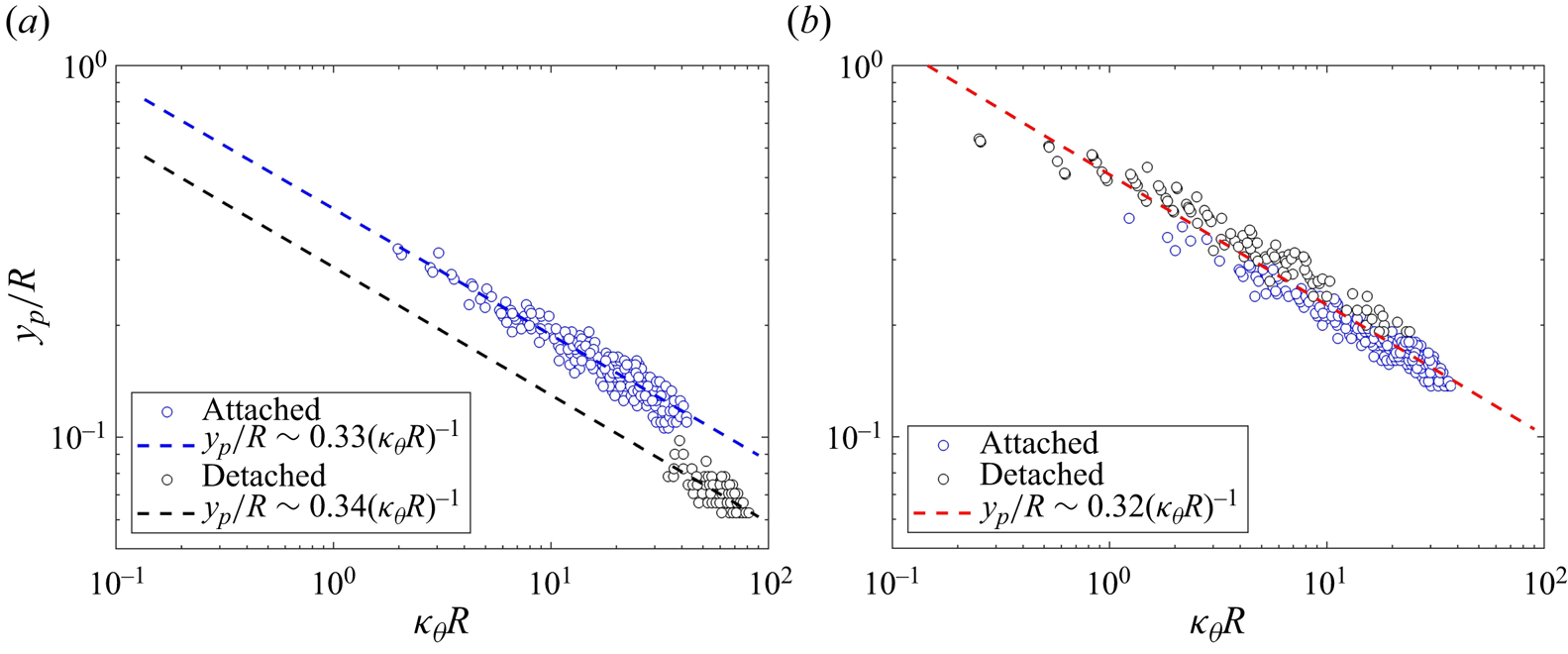
Figure 9.

Modal self-similarity of the POD modes $\hat {\varPhi }_{(q=1,p)}(r)$. Plots (a,b) refer to $Re_\tau =2000$ and $Re_\tau =5200$, respectively. The wall-normal length scale is estimated as radial extension $y_p/R$, with the scaling law $y_p/R \sim C(\kappa _\theta R)^{-1}$ and $C \approx 0.32$. Attached and detached eddies are shown in blue and black, respectively. The dashed lines are obtained via linear regression in the least squares sense for the two sets of points.

This distinction shows that the two clusters of points in figure 9(a) correspond to the two previously extracted classes of modes. Therefore, the black modes do not constitute a set of deviated POD modes but rather a topologically distinct set of modes, i.e. detached modes, which also exhibit self-similarity. In fact, by extrapolating the constant of linear scaling for these two groups individually, it becomes evident that they both exhibit self-similarity, with a similar constant $C \approx 0.3$. This value is in close agreement with the estimation by Hellström et al. (Reference Hellström, Marusic and Smits2016) at $Re_\tau =2460$, where this ‘deviating set of modes’ was excluded since it was not previously identified as detached eddies. Nevertheless, as suggested by Hellström et al. (Reference Hellström, Marusic and Smits2016), this deviation is likely an effect of the low Reynolds number. Therefore, considering that the two classes are not very distinct at $Re_\tau =2000$, as seen in figure 5(a), we also examine the highest Reynolds number, $Re_\tau =5200$, where the two branches exhibit two distinct slopes; see figure 5(b). The set of points converges to a single, overlapping group of modes, showing a slope of $y_p/R \sim 0.32 (\kappa _\theta R)^{-1}$. Figure 9(b) indicates a linear scaling for $\kappa _\theta R \in [0.2,37]$. The most energetic structures located in the logarithmic and outer layers, which were categorised above as attached and detached eddies, clearly exhibit a single azimuthal length scale. The geometric self-similarity of the energy-containing motions, for both attached and detached eddies, is reported here for the first time as it necessitates a high Reynolds number and the subsequent separation of scales. This observation aligns with the findings of Hwang (Reference Hwang2015) for turbulent channel flows and constitutes a fundamental aspect for models based on Townsend's AEH.

4.6. Helix angle of the modes

To comprehensively characterise the spatial arrangements of the attached and detached eddies within the logarithmic layer and above, we measure the dominant helix angle, which represents the azimuthal inclinations relative to the streamwise direction. For this analysis, we exclusively focus on the highest Reynolds number, namely $Re_\tau =5200$, since an adequate separation of scales is needed. When examining instantaneous velocity streaks longer than $3R$ (as shown on the cylindrical shells in figure 1), they frequently exhibit relatively straight configurations, indicating minimal variation in their azimuthal inclinations with respect to the streamwise direction. While they may maintain constant angles on the shell (Baltzer et al. Reference Baltzer, Adrian and Wu2013), these extended streaks can take on the appearance of a helix in the three-dimensional space. Therefore, we now refer to the angle between the streamwise direction within a cross-stream plane ($r, \theta$) as the ‘helix angle’. The helix angle, denoted as $\alpha _h$, can be either positive or negative, depending on whether the helix rotates clockwise or anticlockwise when viewed from a downstream location.

For the POD modes, the helix angle can be measured following the definition by Baltzer et al. (Reference Baltzer, Adrian and Wu2013), where $\alpha _h$ is defined as

(4.1)\begin{equation} \alpha_h \approx \text{arctan} \left( \frac{(R-y)2{\rm \pi} \kappa_z}{L_z \kappa_\theta} \right), \end{equation}

a function of the wall-normal distance $y$, the axial length ($L_z$) and wavenumber ($\kappa _z$). In the current classification, we estimate $\alpha _h$ for each POD mode using the location of the largest peak ($y_p$). In 95.2 % of cases, both classes exhibit a helix angle below $6.5^{\circ }$. This consistency with the helix angles measured in the instantaneous fluctuating axial-velocity structures and the dominant streaks of the two-point correlations by Baltzer et al. (Reference Baltzer, Adrian and Wu2013) is noteworthy. Their study was conducted in a pipe of similar length ($30R$) and moderately high Reynolds number ($Re_\tau =685$). They also performed POD and measured angles of ${\approx }5.1^{\circ }$ and ${\approx }6.8^{\circ }$ for the most energetic modes. The energy-based classification introduced above allows us to observe how the helix angles vary for the specific classes that contribute significantly to the energy, i.e. attached and detached eddies.

The two classes exhibit distinct helical behaviours. The attached eddies, primarily located in the logarithmic region ($y/R<0.3$), consistently exhibit helix angles of less than $3.2^{\circ }$; see figure 10(a). This results from the combination of two effects. First, the size of the attached eddies scales linearly with the wall-normal distance, as discussed earlier, but the peak does not shift significantly toward the centre of the pipe. Additionally, these modes can have large wavelengths; see figure 10(c). When these observations are combined in (4.1), the resulting helical twist remains relatively small (figure 10). In contrast, the detached eddies exhibit significant variability. As mentioned in the previous section, a clear separation between the two classes only occurs at the highest Reynolds number. This could potentially explain why Baltzer et al. (Reference Baltzer, Adrian and Wu2013) did not report larger $\alpha _h$ values among the most energetic modes. The detached eddies maintain an almost constant size regardless of their wall-normal location and have helix angles ranging between $3^{\circ }$ and $7^{\circ }$, with some outliers having a helix angle exceeding $7.5^{\circ }$. The outlier modes do not have an exceptionally long streamwise length, with their axial wavelength always remaining below 5; see figure 10(c). However, they do exhibit a significant shift towards the centre of the pipe with a peak occurring around $y/R \approx 0.5$. This implies that as the eddies detach from the wall while maintaining an almost constant size, they progressively exhibit a larger twisting with an angle of up to $11.2^{\circ }$. This is also evident in figure 11, where we present the POD modes 27 and 7, as examples. The attached eddy in figure 11(a) exhibits a smaller twist, with the streamwise velocity streaks remaining attached to the wall. In contrast, the detached mode in figure 11(b) displays a more pronounced twisting, attributed to a stronger azimuthal velocity.

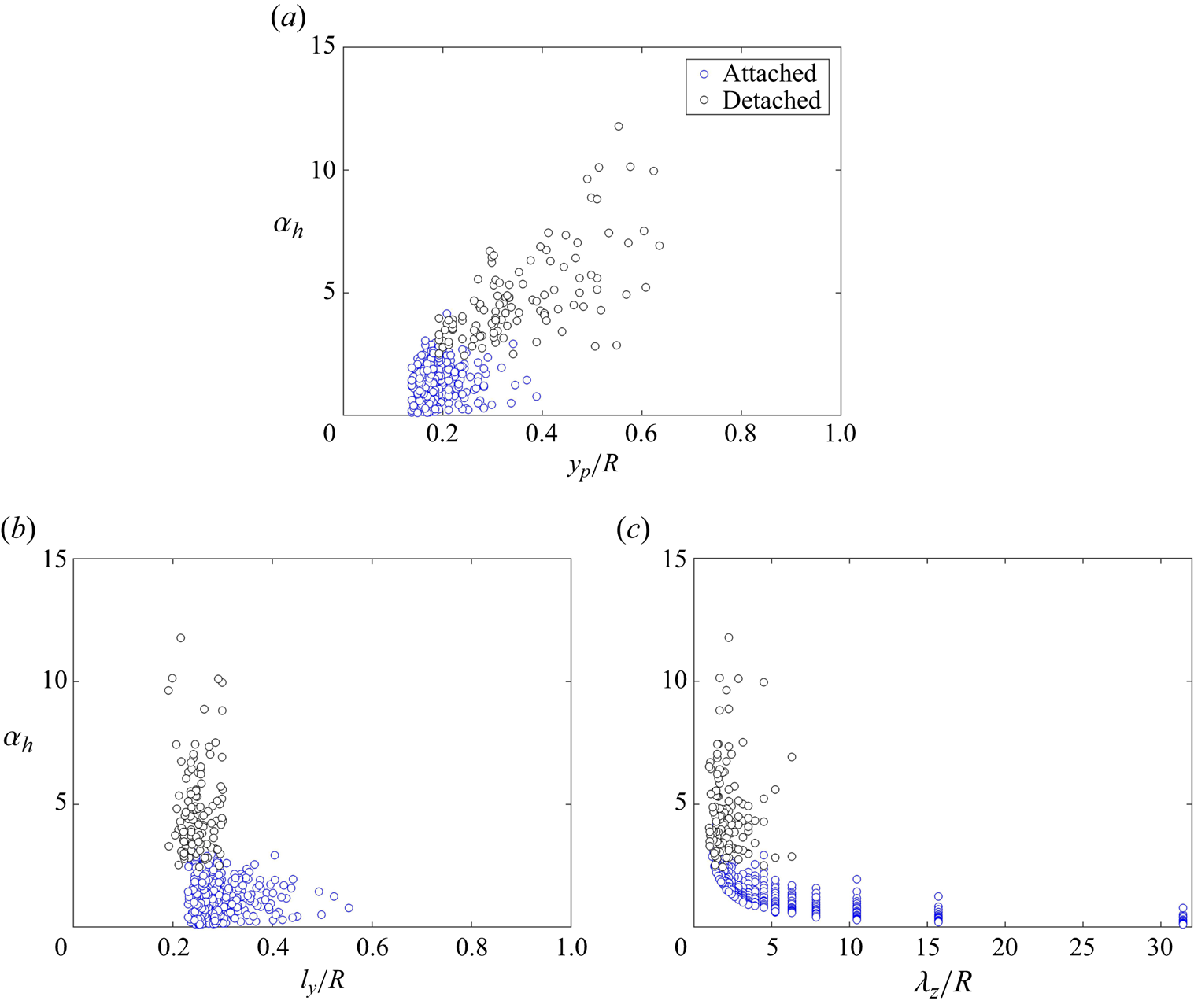
Figure 10.

Helix angle of the attached (blue) and detached (black) POD modes $\hat {\varPhi }_{(q=1,p)}(r)$, as a function of (a) the peak location, (b) the radial size of the mode and (c) the axial extension, i.e. the axial wavenumber. All the panels refer to $Re_\tau =5200$.

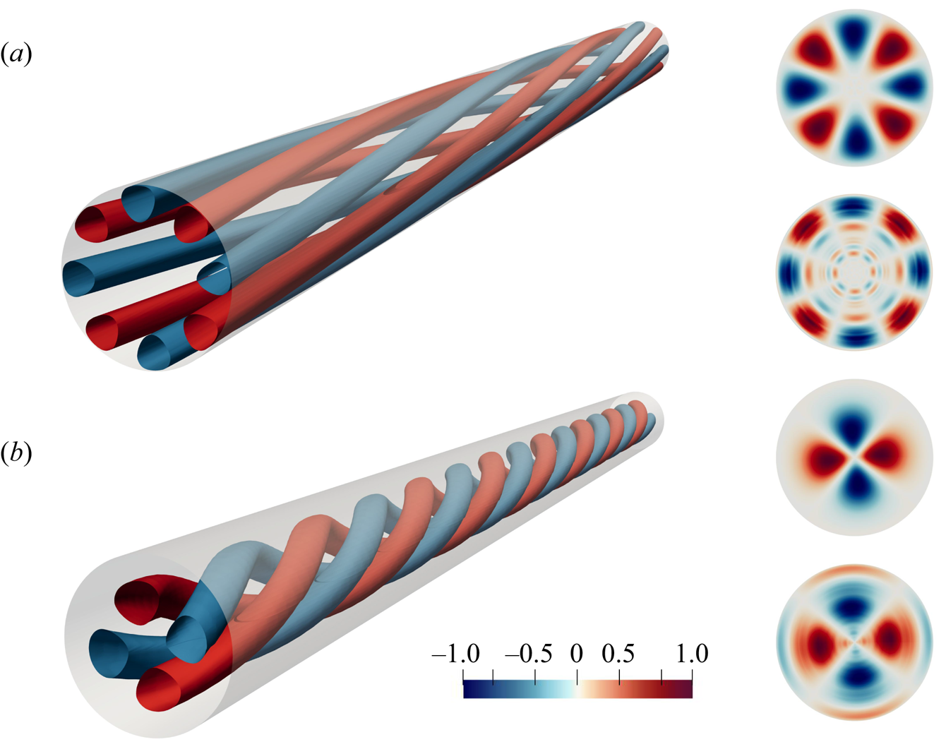
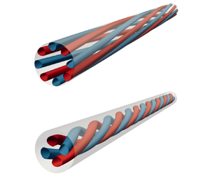
Figure 11.

Illustration of the spatial development and corresponding helical angle for the (a) attached and (b) detached POD mode with wavenumbers ($\kappa _\theta =4$, $\kappa _z=2$) and ($\kappa _\theta =2$, $\kappa _z=7$), respectively. From left to right: positive and negative three-dimensional isosurfaces of the axial velocity $u_z$ (corresponding to 50 % of the maximum magnitude) and cross-stream planes of the radial and azimuthal velocity. Both panels refer to $Re_\tau =5200$.

Thus, the two classes exhibit distinctive helical characteristics. Remarkably, they share similarities with very long fluctuating axial motions and the two-point correlation, as reported in Baltzer et al. (Reference Baltzer, Adrian and Wu2013). However, the POD modes display organised, periodic patterns around the circumference of the pipe. These vector patterns remain consistent for each POD mode as $z$ varies, with the only variation being a rotation around the pipe axis in a helical manner. Note that while the counterclockwise modes are presented in figure 11, there is always an equivalent set of clockwise modes for oppositely signed wavenumbers. The only difference is that the azimuthal variations are mirror images of the illustrated modes. In general, these motions exhibit characteristics resembling roll cells in a statistical sense. As a result, these mode patterns may not appear visually symmetric in the instantaneous planes, especially as they approach the core.

4.7. Large- and very-large-scale motions

Large-scale motions are commonly described as the coalescence of vortex packets generated when multiple structures travel at the same convective velocity (Kim & Adrian Reference Kim and Adrian1999; Adrian et al. Reference Adrian, Meinhart and Tomkins2000; Balakumar & Adrian Reference Balakumar and Adrian2007). In particular, LSMs involve the alignment of vortical structures within the packet in the streamwise direction, leading to the creation of zones with reduced streamwise momentum (Adrian et al. Reference Adrian, Meinhart and Tomkins2000; Ganapathisubramani, Longmire & Marusic Reference Ganapathisubramani, Longmire and Marusic2003). In turbulent pipe flows, LSMs are associated with structures of a size of approximately $3R$ (Baltzer et al. Reference Baltzer, Adrian and Wu2013). In addition to these, energetic modes that are not only longer but also taller have been observed. These ‘VLSMs’ are defined as motions that are longer than the mean bulge length (Jiménez Reference Jiménez1998; Kim & Adrian Reference Kim and Adrian1999). In the outer region of fully developed turbulent pipe flow, VLSMs reach wavelengths well beyond dozens of the pipe radius in length (Guala, Hommema & Adrian Reference Guala, Hommema and Adrian2006; Monty et al. Reference Monty, Stewart, Williams and Chong2007). In this context, our objective is to identify whether the two previously detected classes correspond (or are related) to LSMs and VLSMs. Note that both sets of the POD modes, calculated for $\{N_\theta \times N_z\}=\{32,32\}$, predominantly exhibit their largest peak in the outer layer. Figure 12 illustrates the regions of interest in the current study, which focuses on LSMs. Let us emphasise once more that the transparent light-blue region in figure 12 is not intended as a threshold for filtering, but rather represents an outcome of the energy-based classification.

Figure 12.

(a) Mean velocity profile and (b) wavenumber pre-multiplied energy spectrum $k_\theta E_{zz}/u_\tau ^2$ for $Re_\tau =5200$. The light-blue area refers to the locations where the largest peak of the most energetic modes for $\{N_\theta \times N_z\}=\{32,32\}$ are located.

The distribution of POD modes for each of the two classes is measured in terms of the axial size ($l_z$), the largest peak location ($y_p$) and the beginning/end of the structure. Probability density functions (PDFs) are obtained via histograms (with a constant unitary area for each diagram) and the conclusions drawn in this section are not affected by the binning choice. In figure 13(a) the PDF of the streamwise length is shown ($l_z=10 {\rm \pi}R/\kappa _z$). Note that a distinction is necessary between the streamwise wavelengths defined using the streamwise Fourier decomposition and the streamwise wavelengths defined based on the presence of azimuthal wavering (Baltzer et al. Reference Baltzer, Adrian and Wu2013). In an experimental hot-wire rake measurement of turbulent pipe flow, Monty et al. (Reference Monty, Stewart, Williams and Chong2007) observed exceptionally long streamwise velocity structures, reaching lengths of up to $25R$. These structures exhibited a $180^{\circ }$ rotation about the pipe axis, as well as meandering with large helix angles. This interpretation of sinusoidal meandering is in agreement with the view of attached eddies with high (and almost constant in $y$) helix angles. It is also consistent with the interpretation based on shorter streaks with azimuthal inclinations interacting with a helix angle varying in $z$. Both scenarios can generate two-point correlation patterns consistent with those observed in experiments (Monty et al. Reference Monty, Stewart, Williams and Chong2007; Baltzer et al. Reference Baltzer, Adrian and Wu2013). However, the current energy-based statistical approach makes it impossible to distinguish the two interpretations. An alternative decomposition based on dynamic evolution, such as dynamic mode decomposition (Schmid Reference Schmid2022), might provide additional insights. In that case, identifying the most ‘relevant’ mode becomes critical, as no clear hierarchy is inherently present.

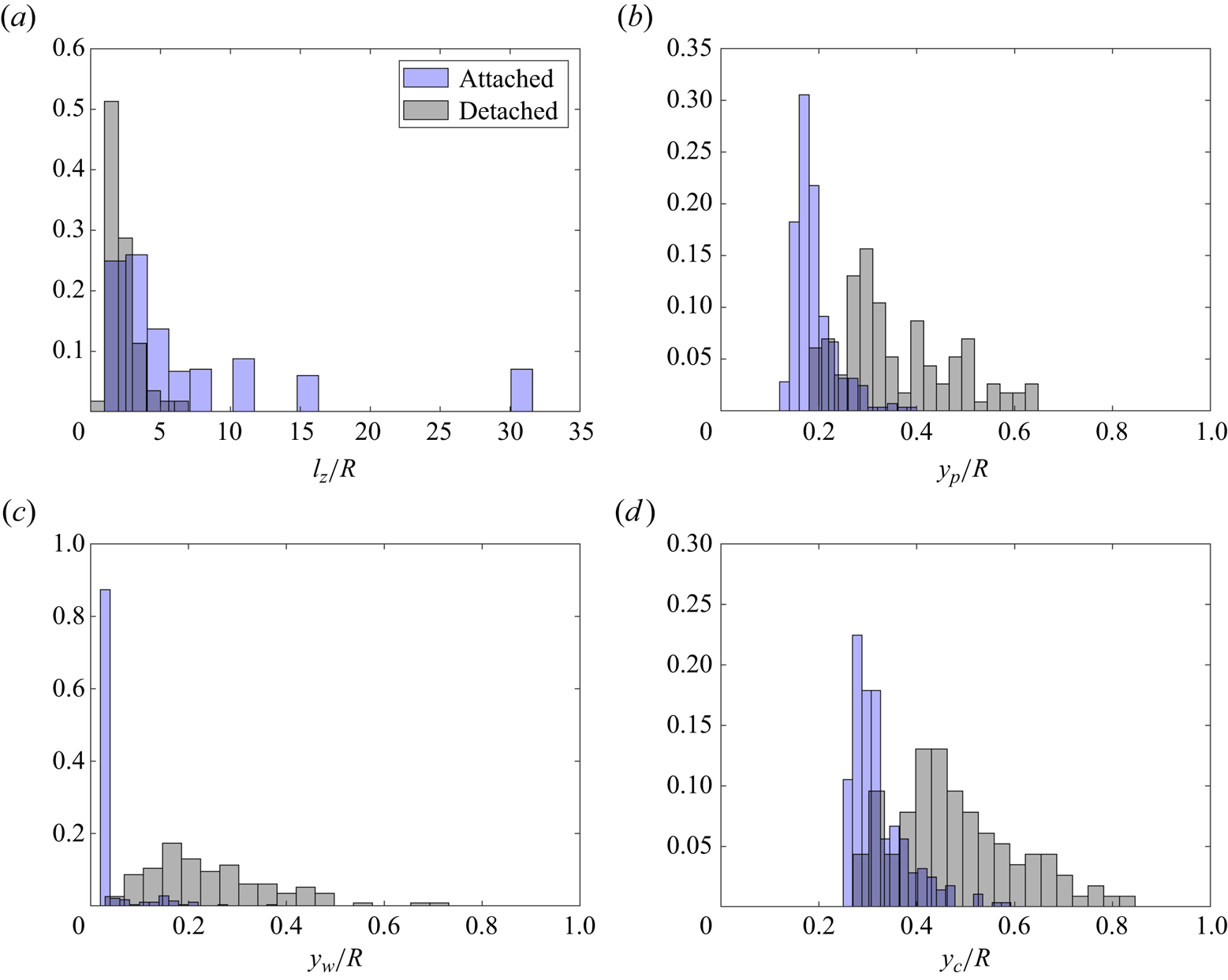
Figure 13.

Discrete PDF of the attached and detached eddies for (a) axial extension, (b) the largest peak location, (c) the beginning and (d) the ending of the POD mode in the radial direction. The blue and black areas are normalised to guarantee a unitary area. All the panels refer to $Re_\tau =5200$.

In this section, our focus is not to delve into the mechanism of VLSM formation. Instead, we aim to quantify the presence of VLSMs and LSMs within the two energetic classes of attached and detached structures. Our findings strongly suggest that the VLSM structures are most likely attached. This conclusion is supported by the observation that all POD modes in class I (see figure 5) exhibit an elongation greater than $3R$ in the axial direction ($\kappa _z < 10$). In contrast, the detached eddies exhibit similarities to LSMs, with approximately 83 % of them having an axial extension smaller than $3R$ ($l_z \lessapprox 3$). The few VLSMs within the detached eddies still have relatively short lengths, ranging from 3.1$R$ to 6.1$R$, whereas the VLSM attached motions consistently exhibit lengths exceeding $8R$; see figure 13(a).

The largest peak location in the radial direction also exhibits an interesting pattern. In the case of attached eddies, i.e. VLSM, approximately 97.8 % of these structures have their peaks in the log region ($y/R < 0.3$), as shown in figure 13(b). Thus, the proposed characterisation outlines the attached nature of these motions; see figure 13(c). The beginning of these structures, denoted by $y_w$, is consistently located near the wall. These VLSMs typically terminate around $0.5R$, not extending far into the pipe's central region (figure 13d), consistently with the modes shown in figure 11. However, this situation changes for the detached motions. Only 33.1 % of them have the largest peak in the log layer, with structures progressively shifting towards the pipe centre. They reach up to a wall-normal distance of approximately 0.8$R$, with their beginnings completely detached from the wall. Figure 13(c) clearly illustrates this detachment as structures become progressively more centralised.