


1. Introduction
Rayleigh–Bénard (RB) convection is the fluid flow driven by the buoyancy forces arising from temperature gradients acting in the direction opposite to gravity. Such a process is almost ubiquitous both in nature and in industrial environments. Examples of natural processes dominated by RB convection are the formation of ocean currents and winds (Rahmstorf Reference Rahmstorf2006), the convection in the Earth's inner core (Glatzmaier & Roberts Reference Glatzmaier and Roberts1995) and plate tectonics (Morgan Reference Morgan1972; Richter Reference Richter1978). Moreover, since the early experiments by Bénard (Reference Bénard1900) and the later theoretical work of Rayleigh (Reference Rayleigh1916), both the experimental and theoretical studies of RB convection have prompted the development of the hydrodynamic stability theories (Chandrasekhar Reference Chandrasekhar1981; Drazin & Reid Reference Drazin and Reid1981) and the basic knowledge on pattern formation in turbulent chaotic flows (Getling Reference Getling1998).
The evolution of RB convection is characterized by the formation of coherent structures, which persist in the regime of strong turbulence and exhibit a complex and chaotic dynamics. In recent years, statistical approaches have been adopted to study the behaviour of such structures both experimentally and numerically (Ahlers, Grossmann & Lohse Reference Ahlers, Grossmann and Lohse2009; Lohse & Xia Reference Lohse and Xia2010; Chillà & Schumacher Reference Chillà and Schumacher2012; Xia Reference Xia2013). This has been possible in the wake of the development of non-intrusive whole-field flow visualization techniques, such as particle image velocimetry (PIV) or laser induced fluorescence (LIF), and the advent of high-speed supercomputers that have enabled the direct numerical simulation (DNS) of highly turbulent flows. The extensive amount of experimental and numerical data gathered in the last years has also promoted further theoretical work aimed at developing theories for the prediction of the global flow transport properties, such as the heat transfer efficiency and the dynamic properties of the mean wind of the turbulent convection.
In order to make experimental and numerical results comparable with each other, most of the latest works have focused on the analysis of RB convection in closed boxes. Therefore, a typical RB system consists of a fluid layer delimited by two horizontal plates, kept at constant temperature and confined by a lateral wall. The fluid is heated from below and cooled from above, whereas the sidewall is typically adiabatic. Moreover, thermal convection is generally studied within the Oberbeck–Boussinesq approximation (i.e. the fluid density is assumed to vary linearly with the temperature). A system of such a kind is effortlessly accessible in a laboratory, as well as easy to reproduce in a numerical environment; furthermore, although less complex than systems occurring in natural phenomena or engineering applications, it preserves the most relevant features of the latter. More specifically, in the following, attention is paid to RB convection inside a cylindrical cell, which is widely addressed in the literature (Ahlers et al. Reference Ahlers, Grossmann and Lohse2009). Such a system is controlled essentially by three dimensionless parameters: the Rayleigh number  $Ra=\beta g {\rm \Delta} T H^{3}/(\nu \alpha )$; the Prandtl number $Pr=\nu /\alpha$; and the cell aspect ratio $\varGamma =D/H$, where $\beta$, $\nu$ and $\alpha$ are the thermal expansion coefficient, kinematic viscosity and thermal diffusivity of the fluid, $g$ is the gravitational acceleration, ${\rm \Delta} T$ is the temperature difference across the fluid layer and $H$ and $D$ are the height and the diameter of the convection cell.
As well known, the convective motion inside the cell originates from an overturning thermal instability of the fluid layer above a critical value of the Rayleigh number. Buoyancy forces cause hot and cold plumes to detach from the boundary layers on the top and the bottom plates and, while moving across the cell, they organize themselves into a large-scale circulatory motion, known as large scale circulation (LSC) (Xi, Lam & Xia Reference Xi, Lam and Xia2004). In most cases, the latter spans the entire height of the cell and has a quasi-planar flywheel structure (Qiu & Tong Reference Qiu and Tong2001). The LSC features a very complex and chaotic behaviour characterized by a multiplicity of dynamical modes, which, however, show periodicity in time. First, the nearly vertical plane of the LSC undergoes continual reorientation in a Brownian fashion, in such a way that a preferential azimuthal orientation does not exist (at least until the cylinder axis forms a negligible angle with the gravity) (Cioni, Ciliberto & Sommeria Reference Cioni, Ciliberto and Sommeria1997; Sun, Xi & Xia Reference Sun, Xi and Xia2005b; Brown & Ahlers Reference Brown and Ahlers2006a,Reference Brown and Ahlersb; Xi, Zhou & Xia Reference Xi, Zhou and Xia2006; Xi & Xia Reference Xi and Xia2007). Such rotation of the LSC plane is associated with torsional oscillations (Funfschilling & Ahlers Reference Funfschilling and Ahlers2004; Funfschilling, Brown & Ahlers Reference Funfschilling, Brown and Ahlers2008) and sloshing oscillations (Xi et al. Reference Xi, Zhou, Zhou, Chan and Xia2009; Zhou et al. Reference Zhou, Xi, Zhou, Sun and Xia2009). The torsional mode consists of out-of-phase azimuthal rotations of the upper and lower parts of the LSC, resulting in a twist of its structure. On the other hand, the sloshing mode consists of a horizontal displacement of the entire LSC away from the cylinder axis and is accompanied by horizontal fluctuations of both velocity and temperature in the bulk. Before the identification of such a mode, these oscillations had been associated with the periodic and alternate emissions of plumes from the opposite boundary layers (Villermaux Reference Villermaux1995). However, the work by Xi et al. (Reference Xi, Zhou, Zhou, Chan and Xia2009) elucidated conclusively that thermal plumes are emitted neither periodically nor alternately, but randomly and continuously, from the top and bottom plates. A further relevant mode of the LSC is the occurrence of cessations and reversals, i.e. abrupt interruptions and changes in the orientation of the circulatory motion (Brown, Nikolaenko & Ahlers Reference Brown, Nikolaenko and Ahlers2005; Brown & Ahlers Reference Brown and Ahlers2006b; Xi & Xia Reference Xi and Xia2007). Cessations and reversals of the thermal convection have been often related and compared to Earth's magnetic pole inversions (Glatzmaier & Roberts Reference Glatzmaier and Roberts1995) and reversals of the wind in Earth's atmosphere (van Doorn et al. Reference van Doorn, Dhruva, Sreenivasan and Cassella2000). This explains the deep interest of the research community in characterizing the statistical properties of their occurrence. Several studies have shown that, after a cessation, any azimuthal orientation has the same probability to occur and, thus, a reversal is only a special case of cessation. Moreover, since cessation events are Poisson distributed in time, successive cessations are statistically uncorrelated (Brown et al. Reference Brown, Nikolaenko and Ahlers2005).
Most of the above results are related to RB convection in cylindrical cells with  $\varGamma =1$. Numerous studies have been also focused on the $\varGamma =0.5$ case, which is of interest for the present work. In $\varGamma =0.5$ cells, the LSC has been observed to have an even richer dynamics, characterized by a periodic switching between different states. In their DNS study, Verzicco & Camussi (Reference Verzicco and Camussi2003) found out the existence of a flow mode consisting of two vertically stacked nearly circular counter-rotating rolls, which were later observed experimentally by Xi & Xia (Reference Xi and Xia2008). Xi & Xia (Reference Xi and Xia2008) revealed random temporal successions of the single-roll state (SRS) and the double-roll state (DRS), with a prevalent occurrence of the DRS as $\varGamma$ is decreased. In Stringano & Verzicco (Reference Stringano and Verzicco2006) a simple model for the prediction of this bimodality was also given. Moreover, Xi & Xia (Reference Xi and Xia2007) showed that cessations and reversals are more frequent in $\varGamma =0.5$ cells than in $\varGamma =1$ cells, although in the later work of Weiss & Ahlers (Reference Weiss and Ahlers2011b) frequencies of such events comparable to those observed in $\varGamma =1$ cells (Brown & Ahlers Reference Brown and Ahlers2006b) were found.
The LSC has been recognized as the first mode (or dipole mode) of the RB convection. In addition to it, higher-order modes have been identified and their role in the events characterizing the evolution of the LSC has been investigated. For a  $\varGamma =1$ cell, $Pr=0.7$ and $Ra$ between $6\times 10^{5}$ and $3\times 10^{7}$, Mishra et al. (Reference Mishra, De, Verma and Eswaran2011) observed the dominance of the second Fourier mode during a cessation/reversal event. Xi et al. (Reference Xi, Zhang, Hao and Xia2016) studied the high-order modes of the flow in a $\varGamma =1$ cell in the range $9\times 10^{8}< Ra<6\times 10^{9}$ and in a $\varGamma =0.5$ cell in the range $1.6\times 10^{10}< Ra<7.2\times 10^{10}$, using water as working fluid with $Pr=5.0$ in both cases. Their results show that in $\varGamma =1$ cells the higher-order modes are very weak compared with the LSC and contain less than $4\,\%$ of the total flow energy, whereas in $\varGamma =0.5$ cells they become stronger, with the second mode containing $13.7\,\%$ of the total flow energy. Moreover, they observed that during a reversal/cessation, the amplitude of the higher-order modes experiences a rapid increase followed by a decrease, which is opposite to the behaviour of the amplitude of the first mode. The relative importance of the higher-order modes has also been studied to assess the persistence of the LSC after cell rotation, tilting or changing to smaller aspect ratio (Kunnen, Clercx & Geurts Reference Kunnen, Clercx and Geurts2008; Stevens, Clercx & Lohse Reference Stevens, Clercx and Lohse2011; Weiss & Ahlers Reference Weiss and Ahlers2011a, Reference Weiss and Ahlers2013).
Apart from the investigation into the behaviour of the coherent structures of the flow, as highlighted by Xia (Reference Xia2013) in his review, other relevant trends in the research on RB convection have pertained to the analysis of turbulent heat transfer, the boundary layer dynamics and the inspection of small-scale turbulence. Such topics are strictly correlated with each other and with the dynamics of the vortex coherent structures. It is straightforward that the transition of the flow to different dynamical states may have an impact on both the global heat transfer and the structure of the boundary layers and of the bulk turbulence (Verzicco & Camussi Reference Verzicco and Camussi2003). The same Grossman–Lohse theory (Grossmann & Lohse Reference Grossmann and Lohse2000, Reference Grossmann and Lohse2001, Reference Grossmann and Lohse2002, Reference Grossmann and Lohse2004), which constituted an attempt to unify experimental and numerical data from the manifold of works available in the literature, relies on the theoretical assumption that the turbulent bulk and the boundary layers on the plates and the lateral wall contribute with different mechanisms (and thus different scaling laws) to the time- and volume-averages of the kinetic and thermal energy-dissipation rates. This leads to a classification of different flow regimes in the  $Ra$–
$Ra$– $Pr$ parametric space, based on the prevalence of one contribution over the other. Each of these regimes corresponds to a different power law of the Nusselt number $Nu =\dot {q}H/(\kappa {\rm \Delta} T)$ (with $\dot {q}$ being the area- and time-averaged total heat flux across any horizontal section of the cell and $\kappa$ being the fluid thermal conductivity) and the Reynolds number $Re =WH/\nu$ (where $W$ is a characteristic velocity scale of the turbulent motion) as functions of $Ra$ and $Pr$. On the other hand, several works (Funfschilling et al. Reference Funfschilling, Brown, Nikolaenko and Ahlers2005; Nikolaenko et al. Reference Nikolaenko, Brown, Funfschilling and Ahlers2005; Sun et al. Reference Sun, Ren, Song and Xia2005a) have shown that $Nu$ has a weak dependence on $\varGamma$ in both cylindrical and rectangular samples. This would suggest an insensitivity of the heat flux to the actual configuration of the coherent vortex structures present in the flow field. As concerns the main results about the structure of the small-scale thermal turbulence and, in particular, the existence of a Bolgiano–Obukhov scaling, the reader is referred to the comprehensive review of Lohse & Xia (Reference Lohse and Xia2010).
In conclusion of the present overview, it is worth remarking that, while theoretical and numerical studies generally address only the influence of the above-mentioned parameters ( $Ra$,
$Ra$,  $Pr$ and $\varGamma$) on the thermo-fluid-dynamic properties of RB convection, further effects might have a relevance in laboratory tests, as a consequence of imperfections and non-idealities of the experimental set-up. Among them, the finite conductivity of the bottom and top plates of the cell and the never-perfect adiabaticity of the lateral wall can limit the global heat transfer and also affect the flow dynamics (Ahlers Reference Ahlers2000; Roche et al. Reference Roche, Castaing, Chabaud, Hébral and Sommeria2001; Hunt et al. Reference Hunt, Vrieling, Nieuwstadt and Fernando2003; Niemela & Sreenivasan Reference Niemela and Sreenivasan2003; Verzicco Reference Verzicco2004; Stevens, Lohse & Verzicco Reference Stevens, Lohse and Verzicco2014). In principle, the thermal conductivity of the plates $\kappa _p$ is required to be much larger than the effective thermal conductivity of the flow $\kappa Nu$, otherwise the emission of a plume results in a deficiency or excess of enthalpy that leaves a cold or warm spot on the plate where the probability of a new plume emission is diminished, until the spot itself is diffused away. Hunt et al. (Reference Hunt, Vrieling, Nieuwstadt and Fernando2003) observed that such mechanisms have a great impact on the flow structures, leading to the formation of elongated plumes when $\alpha _p\ge \alpha$ and, vice versa, small-scale puffs when $\alpha _p\le \alpha$, with $\alpha _p$ being the thermal diffusivity of the plates. If the finite conductivity of the plates is relevant for large $Ra$, the sidewall properties affect the thermal convection only at small or moderate values of $Ra$. Specifically, even when perfectly isolated on the external side, the presence of a sidewall results in a heat current that circumvents the fluid layer, entering the wall in the bottom half of the cell and exiting it in the top half. However, this coupling between the sidewall and the convecting fluid has only a minor effect on the global heat transfer, even though it can significantly affect the structure and intensity of the LSC (Niemela & Sreenivasan Reference Niemela and Sreenivasan2003). Stevens et al. (Reference Stevens, Lohse and Verzicco2014) also showed that the nature of the thermal boundary condition (constant temperature or adiabatic surface) at the external side of the sidewall can determine different flow organizations and, correspondingly, different heat transport. In the case of an isothermal boundary condition, they showed that a difference between the temperature imposed at the external side of the sidewall and the volume-averaged temperature of the fluid can introduce asymmetries in the flow and the heat transfer rates at the two opposite plates.
The present paper reports on an experimental study of thermal convection inside a cylinder with  $\varGamma =0.5$ via time-resolved PTV. Differently from previous investigations in the field, velocity measurements are carried out over the whole interior of the cylindrical cell for a very long time. This allows us to provide insight into the instantaneous complex dynamics of RB convection and the statistical properties of its characteristic modes. For this purpose, most of the previous studies have relied on the multithermal-probe approach (Funfschilling et al. Reference Funfschilling, Brown, Nikolaenko and Ahlers2005, Reference Funfschilling, Brown and Ahlers2008; Brown & Ahlers Reference Brown and Ahlers2006a) or punctual or planar velocity field measurements (Sun et al. Reference Sun, Xi and Xia2005b; Sun, Xia & Tong Reference Sun, Xia and Tong2005c; Xi & Xia Reference Xi and Xia2008) performed via laser Doppler anemometry (LDA) or PIV. Experimental works featuring three-dimensional (3-D) measurements of the velocity field are almost rare. Worthy of mention are: the works by Gasteuil et al. (Reference Gasteuil, Shew, Gibert, Chilla, Castaing and Pinton2007) and Shew et al. (Reference Shew, Gasteuil, Gibert, Metz and Pinton2007), who used small buoyant capsules equipped with temperature sensors, an on-board battery and a signal emitter (smart particles) to both track the flow trajectories and measure heat flux along them; the PTV study of Ni, Huang & Xia (Reference Ni, Huang and Xia2012); the simultaneous velocity and temperature measurements of convection in a rectangular box by Schiepel, Schmeling & Wagner (Reference Schiepel, Schmeling and Wagner2016). In not one of these investigations, however, have 3-D measurements been performed in the whole domain of the turbulent convection or for a duration of time sufficiently long enough to obtain reliable turbulent statistics. In the present experiment, the working fluid is water and the Rayleigh number and Prandtl numbers are equal to $1.86\times 10^{8}$ and $7.6$, respectively, the cylinder height is $H=148$ mm and the experiments are carried out for approximately four hours. The aim of the present measurements is to provide a full-field visualization of the characteristic modes of the turbulent convection and a statistical description of their behaviour across the time by using the proper orthogonal decomposition (POD) technique. In the literature on RB convection, a systematic POD analysis has been carried out for rectangular cavities (Verdoold, Tummers & Hanjalić Reference Verdoold, Tummers and Hanjalić2009; Podvin & Sergent Reference Podvin and Sergent2012, Reference Podvin and Sergent2015, Reference Podvin and Sergent2017) or cubic cells (Soucasse et al. Reference Soucasse, Podvin, Rivière and Soufiani2019), whereas very few attempts have been made in the case of cylindrical samples (e.g. Bailon-Cuba, Emran & Schumacher Reference Bailon-Cuba, Emran and Schumacher2010). In the current work, the relationship between the POD modes and the recurring states of the LSC circulation is deeply investigated and innovative criteria for the classification of the flow state based on the POD analysis are introduced and proved to be more effective than methods classically used in the literature and relying on the analysis of the azimuthal profiles of the temperature or the vertical velocity at three different levels (Funfschilling et al. Reference Funfschilling, Brown, Nikolaenko and Ahlers2005; Brown & Ahlers Reference Brown and Ahlers2006a; Xi & Xia Reference Xi and Xia2007, Reference Xi and Xia2008; Funfschilling et al. Reference Funfschilling, Brown and Ahlers2008; Stevens et al. Reference Stevens, Clercx and Lohse2011; Weiss & Ahlers Reference Weiss and Ahlers2011b). The paper is organized as follows. In § 2 the experimental set-up and techniques are described. In §§ 3–5 the main results are presented and discussed. Finally, in § 6, conclusions are drawn.
2. Experimental set-up and techniques
2.1. The convection cell
A sketch of the experimental apparatus is reported in figure 1. The convection cell consists of a Plexiglas cylinder filled with water. The internal diameter of the cylinder is  $D=74$ mm, the aspect ratio is $\varGamma =0.5$ (height equal to twice the internal diameter) and the sidewall thickness is $3$ mm. The cylinder is immersed in an octagonal tank, also filled with water.
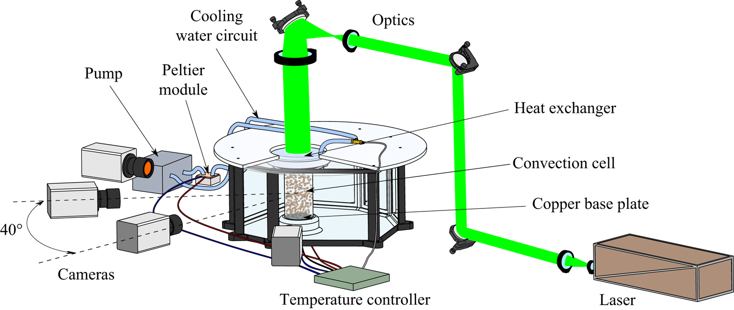
Figure 1. Schematic of the experimental apparatus.
The water inside the cylinder is heated from below and cooled from above by thermal sources kept at constant temperature throughout the duration of the experiment via a high-precision thermoelectric controller (TEC). The bottom heating system consists of an electrolytic copper slab connected to a mica-insulated flat heater, which can provide heating power up to  $100$ W. The copper slab is made of two parts, glued to each other via a highly conductive epoxy, in-between which a PT100 1/10-DIN RTD sensor is placed. The distance of the sensor from the slab surface in contact with the fluid is $12$ mm; due to the large thermal conductivity of the copper, the temperature drop across this layer is negligible with respect to the sensor accuracy. The copper slab is housed in an appropriate site on the bottom of the tank, and the cylinder is fastened to the copper insert with an interference fit. The cylinder sidewall is in contact with the copper insert for a depth of approximately $20$ mm.
The top cooling system consists of a water heat exchanger obtained by assembling a set of Plexiglas layers. These layers comprise two recirculation chambers with nearly opposite tangential inlet and outlet, delimited by a thin slab with a small central hole. The lower recirculation chamber is separated by the convection cell via an acrylic foil of 0.25 mm thickness, which offers a small thermal resistance. The water is refrigerated by a Peltier thermoelectric cooler and pumped into the lower recirculation chamber. The cooler consists of a copper waterblock coupled with a Peltier element, connected to a heat sink with fan, with a maximum heating/cooling power of  $118$ W and a maximum allowable temperature difference between its sides of $\pm 75\,^{\circ }$C. The tubes of the water circuit are coated with neoprene rubber so as to limit heat losses due to heat transfer with the surrounding ambient. The water temperature is measured at the heat exchanger inlet by means of an immersion ultraprecise PT100 1/10-DIN RTD sensor.
Based on the continual measurements from the two resistance temperature detection (RTD) sensors, the thermoelectric controller performs a proportional–integral–derivative control by adjusting the current inputs to the flat heater and the Peltier element and ensures a temperature stability of  $0.01\,^{\circ }$C. Since the temperature difference between the top and the bottom plates is $5\,^{\circ }$C in the present experiments, this corresponds to a percentage stability of the imposed unstable temperature gradient of $0.2\,\%$. The laboratory room with the tank is air conditioned, and maintained at constant temperature; the water temperature is measured by means of an immersion PT100 1/10-DIN RTD probe to check that it remains constant and near to the ambient temperature. The latter is equal to $17.5\,^{\circ }$C; being the nominal temperature difference equal to $5\,^{\circ }$C, the nominal temperature of the bottom is $20\,^{\circ }$C, while the nominal temperature of the top is $15\,^{\circ }$C. The tank temperature during the present experiment is $17.35\,^{\circ }$C.
2.2. Imaging system and camera calibration
The imaging system consists of a dual pulse Nd:YAG laser with maximum pulse energy of  $200$ mJ and four sCMOS cameras (Andor Zyla) with a resolution of $2560\times 2160$ pixels. The laser light is shaped into a cylindrical beam that is passed through the transparent heat exchanger on the top of the cell and illuminates the entire convection domain. The cylindrical shape is obtained by using an appropriate system of mirrors and lenses, as shown in figure 1.
The four cameras are arranged in a planar configuration with an angular spacing of approximately  $40^{\circ }$. In order to focus the whole cylinder interior, each camera is equipped with $28$ mm focal length objectives set at an f-number equal to $22$. The resulting digital resolution is $14$ pixel mm $^{-1}$.
The seeding particles are orange fluorescent polyethylene microspheres (Cospheric UVPMS-BO-1.00); the average particle diameter is  $58\ \mathrm {\mu }$m, while the particle density is $1.00$ g cm $^{-3}$, resulting in a relaxation time lower than $1$ ms (which is significantly below the turbulent dissipative time scales of the thermal convection at the currently investigated conditions). The working fluid is seeded before placing the cylinder in situ and it is not possible to add further seeding particles after the beginning of the experiment. Fluorescence of the particles is exploited to reduce the green reflections from the copper base and increase the particle scattering contrast in the recorded images. For this purpose, the camera lenses are equipped with HOYA YA3 orange filters.
Optical calibration of the camera system is a critical point of the present experimental set-up, because of inaccessibility of the cylinder interior and optical distortions caused by the curvature of the sidewall. As is well known, such distortions depend on the ratio of the refractive indexes of the sidewall material (Plexiglas) and the surrounding fluid (water) and vary locally with the viewing direction. Specifically, in the present arrangement, the regions affected by the largest optical distortions are those adjacent to the cylinder sidewall, where classical camera models, such as the pinhole-camera model (Tsai Reference Tsai1987; Heikkila & Silven Reference Heikkila and Silven1997; Zhang Reference Zhang2000), do not provide a satisfactory quality of the tomographic reconstruction of the particle distribution. This issue is obviated by using a perspective camera model with a refraction correction for cylindrical distortion based on Snell's law of refraction. All the relevant details about this method are given in Paolillo & Astarita (Reference Paolillo and Astarita2020). The main strengths of the refractive camera model are the limited number of parameters involved (which all have a clear physical or geometrical meaning and thus are easily checkable) and the possibility of calibrating such parameters without placing a calibration target inside the cylindrical cell (for this purpose, it is sufficient to record images of the target with the cylinder interposed between the cameras and the target itself). The refractive camera model is initially calibrated following the procedure explained in Paolillo & Astarita (Reference Paolillo and Astarita2020); subsequently, both the pinhole camera and the cylinder parameters are refined and optimized via the volume self-calibration technique (Wieneke Reference Wieneke2008; Discetti & Astarita Reference Discetti and Astarita2014).
2.3. Data acquisition and processing
Once the temperature difference between the top and the bottom is set, the system is allowed to settle for approximately two hours before starting the experiment. Then, measurements are carried out over approximately four hours with a sampling frequency of  $7.5$ Hz. The image analysis consists essentially of three stages: image preprocessing; time-resolved motion analysis; velocity data post-processing.
Time-resolved motion analysis is based on a combination of the most recent algorithms for particle motion tracking and consists essentially of two steps. Initially, a first set of snapshots (typically 5–10) is processed with the sequential-motion-tracking enhancement (SMTE) algorithm (Lynch & Scarano Reference Lynch and Scarano2015); at this stage, multiple iterations of the SMART (Atkinson & Soria Reference Atkinson and Soria2009) and CSMART (Ceglia et al. Reference Ceglia, Discetti, Ianiro, Michaelis, Astarita and Cardone2014; Castrillo et al. Reference Castrillo, Cafiero, Discetti and Astarita2016) algorithms are carried out with a multiresolution approach (Discetti & Astarita Reference Discetti and Astarita2012a); multipass volumetric cross-correlations are performed via an efficient algorithm using sparse matrices (Discetti & Astarita Reference Discetti and Astarita2012b). In the second phase of the process, the STB method (Schanz, Gesemann & Schröder Reference Schanz, Gesemann and Schröder2016) is used for particle tracking. Particle triangulation is performed by the iterative particle identification method (Wieneke Reference Wieneke2012), while the forward-time projection of particles is based on both the extrapolation of known trajectories and cross-correlation techniques.
The output of the above process consists of the particle tracks. The velocity data processing step is aimed at estimating the instantaneous velocity fields from the particle trajectories. This implies the estimation of the particle velocities and the interpolation of the latter onto a structured grid. In the present experiments, a fourth-order polynomial fitting based on a kernel of seven time positions of the particles was used to calculate the particle velocities. The employed kernel, with the current sampling frequency, corresponds to a time interval of  $0.66$ s, which is smaller than the Kolmogorov time scale, estimated to be approximately $1.8$ s for the current experimental conditions. The latter estimate is based on the computation of the time- and volume-averaged turbulent kinetic energy dissipation rate from the theoretical relation $\varepsilon _u=\nu ^{3}H^{-4}(Nu -1)RaPr^{-2}$ (Ahlers et al. Reference Ahlers, Grossmann and Lohse2009), which indeed is exact for cylindrical cells with adiabatic sidewalls. The Nusselt number $Nu$ in the previous formula has been estimated from separate numerical simulations of thermal convection accounting for the presence of the cylinder sidewall and performed with the same code used in Stevens et al. (Reference Stevens, Lohse and Verzicco2014); for all the relevant details about the numerical procedure the reader is also referred to the works of Verzicco & Orlandi (Reference Verzicco and Orlandi1996) and of Verzicco & Camussi (Reference Verzicco and Camussi1999, Reference Verzicco and Camussi2003). As concerns the interpolation of the particle velocities onto a structured grid (i.e. transformation from a Lagrangian reference frame to an Eulerian one), it is based on least-squares polynomial fitting of local data. More specifically, a structured (Cartesian or cylindrical) grid is chosen within the measurement volume; for each point of the grid, particles falling within a fixed search radius are identified and the velocities of such particles are used to determine a local polynomial fitting function which is then evaluated at the location of the grid point. Moreover, to reduce the effects of ghost particles on the determination of the velocity field, only particles with trajectories longer than a fixed number of time instants are used in the above procedure. For the results reported in the following, the employed grid is cylindrical and consists of 71, 38 and 98 nodes in the axial, radial and azimuthal directions, respectively. Each velocity vector in this grid is computed with a second-order polynomial fit on the particle velocities within a search radius of $30$ voxels (approximately $2$ mm) and relying only on the particles with trajectories longer than seven sampling periods. The uncertainty of the present velocity measurements is estimated to be approximately $2\,\%$ of the root mean square of the vertical velocity over the time and the cell volume (which is approximately $0.04w_0$).
2.4. POD
The POD, also known as the Karhunen–Loève method, is a statistical method aimed at finding a basis for modal decomposition from an ensemble of signals (Berkooz, Holmes & Lumley Reference Berkooz, Holmes and Lumley1993). The POD provides a linear decomposition that is optimal from an energetic viewpoint; this means that there is no further linear decomposition that approximates – in a least squares sense – the signal better than the POD when truncated at a specified order (lower than the number of the signal degrees-of-freedom). In the investigation of complex turbulent flows, the POD has been applied for the identification of the most energetic coherent structures since the seminal paper of Lumley (Reference Lumley1967). In 3-D unsteady flows, the POD modes of the velocity field  $\underline {u}(\underline {x},t)$ are sought as the functions $\underline {\phi }(\underline {x})$ that maximize their projection on the velocity field itself. This leads to the following eigenvalue problem:
 \begin{equation} \int_V \overline{\underline{u}(\underline{x},t) \underline{u}(\underline{x}',t)} \underline{\phi}(\underline{x'})\, {\textrm{d}} \underline{x'}=\lambda \underline{\phi}(\underline{x}),\end{equation}
where  $V$ is the cell volume, the symbol $\overline {(\cdot )}$ indicates the statistical average, $\lambda$ is the eigenvalue corresponding to the eigenfunction $\underline {\phi }(\underline {x})$ and $\overline { \underline {u}(\underline {x},t) \underline {u}(\underline {x}',t) } \underline {\phi }(\underline {x'})=\sum _{j=1}^{3} \overline { \underline {u}(\underline {x},t)u_j(\underline {x}',t) } \phi _j(\underline {x'})$. When working with discrete measurements, the integral equation (2.1) turns into the following linear eigenvalue problem:
 \begin{equation} \boldsymbol{C}_{\boldsymbol{U}}\boldsymbol{\phi}= \lambda\boldsymbol{\phi},\end{equation}
where  $\boldsymbol {C}_{\boldsymbol {U}}=1/(N_s-1)\boldsymbol {U}\boldsymbol {U}^{\mathrm {T}}$ is the velocity covariance matrix with $\boldsymbol {U}$ being the observation matrix $\boldsymbol {U}=[\boldsymbol {u}_1,\boldsymbol {u}_2,\dots ,\boldsymbol {u}_{N_s}]$. Each observation $\boldsymbol {u}_i$ includes the set of the measurements of the three velocity components for the $i$th snapshot; thus, the size of $\boldsymbol {U}$ is $3 N_p \times N_s$, where $N_p$ is the number of measurement points and $N_s$ the number of snapshots employed for the computation of the POD modes.
Since the number of grid points is significantly larger than the number of snapshots used for the computation of the POD modes (in the present case  $N_p=264,404$ and $N_s=2,350$), the eigenvalue problem (2.2) is solved via the so-called method of snapshots, first introduced by Sirovich (Reference Sirovich1987). Such a method allows a reduction of the problem size from $3 N_p\times 3 N_p$ to $N_s \times N_s$ and thus it is computationally advantageous. It is also worth remarking that in the discrete form (2.2), the POD reduces to the singular value decomposition (SVD); in the present case, singular value decomposition algorithms are used to apply the method of snapshots.
The POD has been performed by using a subset of all the available snapshots, which covers the two central hours of the experiment. Moreover, only one in every 25 consecutive snapshots is considered for a total of  $2350$ samples. Based on the value of the integral time scales computed from the autocorrelation functions of the three velocity components, the number of statistically independent samples is estimated to be approximately a quarter of the number of employed samples. The uncertainty associated with the POD results reported in the following has been estimated by repeating the same analyses with a different number of samples used for the computation of the POD modes. This resulted in a relative uncertainty up to $7\,\%$.
3. Structure of the mean velocity field and its relationship with the instantaneous evolution
The morphology of the time-averaged velocity field is shown in figure 2; this is obtained by averaging the velocity snapshots over the whole duration of the experiment. In figure 2(a) the isosurfaces of the vertical velocity component corresponding to the values  $\pm 0.026 w_0$, with $w_0$ being the free-fall velocity $w_0=\sqrt {\beta {\rm \Delta} T g H}$ ( $=38.2$ mm s $^{-1}$ in the current case), are represented; in addition, two annular vortex structures (white isosurfaces) are identified and displayed using the $Q$-criterion (Hunt, Wray & Moin Reference Hunt, Wray and Moin1988; Kolar Reference Kolar2007). Figure 2(b) reports the velocity map in the $yz$-plane; here, the magnitude of the velocity vectors is coded in their length, while the colour is representative of the value of the $z$-component (vertical velocity). Previous experimental and numerical investigations (Verzicco & Camussi Reference Verzicco and Camussi2003; Sun et al. Reference Sun, Xi and Xia2005b; Tsuji et al. Reference Tsuji, Mizuno, Mashiko and Sano2005) reported an azimuthally symmetric structure of the mean flow field. Such a result is substantially confirmed by the present measurements; on the other side, minor detectable asymmetries are mainly ascribed to imperfections of the experimental set-up, such as misalignment of the cell axis with respect to the vertical direction, imperfections in geometry, etc. In addition, the asymmetries may also be associated with the chaotic nature of the turbulent convection, which might require a time longer than the duration of the experiment to achieve symmetry in the average.
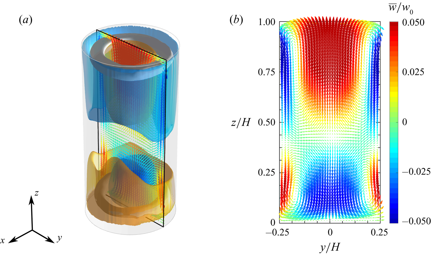
Figure 2. Mean velocity flow field: (a) isosurfaces of vertical velocity corresponding to the values  $\pm \,0.026 w_0$ (yellow and cyan surfaces for the positive and the negative value, respectively) and isosurfaces of the scalar quantity $Q$ corresponding to $0.1$ of the maximum value (white surfaces); (b) velocity vector map in the $yz$-plane. The velocity magnitude is coded in the vector length, while the colour indicates the value of the vertical velocity (scaled by the free-fall velocity $w_0$).
The time-mean flow field is characterized by two separate and opposite radial recirculations extending over the lower and the upper part of the convection cell. In the lower part, the flow is observed to rise up in the regions adjacent to the sidewalls and fall down in the middle; a specular behaviour occurs in the upper part. Such recirculations are associated with the two toroidal vortex structures found in the proximity of the top and bottom plates and shown in figure 2(a). From figure 2(b) it is evident that the recirculation localized in the upper part covers a wider portion of the convection cell than that localized in the lower part. More specifically, the two recirculations are separated by a saddle point on the cylinder axis which is located at  $z/H\approx 0.43$. This is in disagreement with the findings of previous studies (cf. Sun et al. Reference Sun, Xi and Xia2005b), where the saddle point was found at middle height. The present behaviour is associated with an influence of the heat transfer between the fluid sample and the external ambient on the internal dynamics. In fact, in the present experiment, the cylinder sidewall is not perfectly adiabatic and the temperature in the tank $T_e$ (temperature at the external side of the cylinder sidewall) was measured and found to be lower than the average temperature $T_m$ between the top and the bottom of the cell. More specifically, in the investigated case $T_e=17.35\,^{\circ }$C and $T_m=17.5\,^{\circ }$C. Indeed, when $T_e< T_m$ the hot plumes detaching from the boundary layer on the bottom plate and moving near the sidewall lose their heat excess faster than the cold plumes, since they are subjected to a greater heat transfer with the external ambient across the sidewall; thus, the hot plumes are carried into the bulk motion earlier (i.e. at a smaller distance from the bottom plate) with respect to the case $T_e=T_m$ or the case of a cell with an adiabatic sidewall (cases typically investigated in the literature).
The enclosed recirculations present in the time-averaged flow field are not observed in the unsteady evolution. Conversely, the flow organizes in ascending and descending currents which cross the entire cell from one plate to the opposite one. This is clearly visible in the instantaneous velocity maps of figure 3. In both the selected snapshots, plumes rising from the bottom plate or falling from the top plate emerge in the proximity of the cylinder sidewall. In the bottom half of the cell, the emerging hot plumes agglomerate on one side and form a vigorous current which is pushed by buoyancy forces towards the top plate; this current moves near the sidewall for approximately three-quarters of the cell height, then impinges the cold plumes detached from the top, deviates from the sidewall to the centre of the cell and finally reaches the top plate. An analogous behaviour is observed for the cold plumes on the diametrically opposite side of the cell in the top half. Vice versa, the hot/cold plumes which are impeded by opposing descending/ascending currents in their vertical motion are either deviated azimuthally or pushed back; as a consequence, confined recirculations are formed close to the cylinder corners.

Figure 3. Instantaneous velocity vector maps (a) in the  $xz$-plane and (b) in the $yz$-plane corresponding to two different snapshots. The velocity magnitude is coded in the vector length, while the colour indicates the value of the vertical velocity (scaled by the free-fall velocity $w_0$).
The spatial structure and evolution of the ascending and descending currents are in general very complex and are variable across the time. In both the snapshots of figure 3, opposite currents are localized in the same azimuthal plane, thus forming an LSC that exhibits an elliptical structure inclined with respect to the cylinder axis with two counter-rotating rolls in the corners where the currents deviate from the sidewall. However, different states of the turbulent convection are observed in the unsteady evolution. Figure 4 reports, for instance, a snapshot in which the flow appears to be organized in two counter-rotating vertically stacked rolls, localized in the lower and the upper half of the cell. In this configuration, the vertical currents moving along the sidewall travel just one half of the cell height before deviating and going backwards. As aforementioned, such a state is typically referred to as DRS in opposition to the SRS which essentially consists of the domain-filling LSC. The occurrence of the DRS in a cylinder with  $\varGamma =1/2$ was first found numerically by Verzicco & Camussi (Reference Verzicco and Camussi2003) and subsequently observed in several experimental investigations (e.g. Xia, Sun & Cheung Reference Xia, Sun and Cheung2008; Weiss & Ahlers Reference Weiss and Ahlers2011b).

Figure 4. Snapshot of the velocity field in the DRS: velocity vector map in the  $xz$-plane. The velocity magnitude is coded in the vector length, while the colour indicates the value of the vertical velocity (scaled by the free-fall velocity $w_0$).
In order to better identify the characteristic states of the turbulent convection in the unsteady evolution, a POD (Berkooz et al. Reference Berkooz, Holmes and Lumley1993) of the fluctuating part of the velocity field is presented in the next section.
4. Characteristic modes of the turbulent convection
Figure 5 reports the normalized energy spectrum of the POD modes for the first 200 modes. It is worth noting that the normalized energy levels of the POD modes represent the percentage contributions to the average kinetic energy of the fluctuating velocity field, i.e. to the turbulent kinetic energy. The energetic budget of the first modes is not very large compared with that of the high-order modes. The first mode retains only  $6.7\,\%$ of the turbulent kinetic energy, while the sum of the energies of the first 200 modes amount to approximately $87\,\%$, and the energy of the 200th mode is $0.0079\,\%$ of that of the first mode. This is evidence of the absence of statistically dominant modes in the turbulent flow evolution. A closer look at the inset of figure 5 reveals a pairing of the energy levels for the first and the second mode (which amount to $6.7\,\%$ and $6\,\%$ of the total, respectively), as well as for the third and the fourth mode ( $4.4\,\%$ and $4\,\%$) and for the fifth and the sixth mode ( $3.2\,\%$ and $3\,\%$). These pairs of modes share also the same flow structure, except for a $90^{\circ }$ rotation about the cylinder axis, as shown below.

Figure 5. The POD spectrum of the fluctuating velocity field. Energy of the first 200 modes normalized by the total amount of energy. The inset shows the semilogarithmic plot of the normalized energy for the first 50 modes.
The flow morphology of the first and the second POD mode is shown figure 6. In both modes, it is possible to observe the presence of two vertical currents forming a domain-filling circulation. This single roll (SR) has a quasi-planar structure and is not tilted with respect to the cylinder axis. In addition, four small counter-rotating rolls are observed in the corners between the SR and the top and bottom plates (see figure 6c). It is evident that the first two POD modes mainly contribute to the SRS of the LSC observed in the present experiment and in numerous previous experimental and numerical investigations over different ranges of the control parameters. A remarkable difference between the SR of the first two POD modes and the instantaneous LSC in the SRS is the significant inclination of the latter with respect to the cylinder axis, which is visible in figure 3 and was also observed in previous works (Sun et al. (Reference Sun, Xi and Xia2005b), to cite one). Indeed, the inclination of the instantaneous LSC results from the combination of the mean velocity field (see figure 2) and the contribution from the first two POD modes. In fact, this leads to a strengthening of the rising hot plumes and a weakening of the falling cold plumes near the sidewall on the side of the ascending current of the SR and vice versa on the side of the descending current. As a consequence, two of the four rolls observed in figure 2(b) merge in the plane of the SR structure and form an elliptic LSC, while the other two originate counter-rotating rolls at the diagonally opposite corners, as observed experimentally by Sun et al. (Reference Sun, Xi and Xia2005b). Far from the SR plane, the flow is not significantly affected by its dynamics, so, after the superimposition of the contribution from the POD modes 1–2 to the mean flow field, the pattern in the plane normal to the SR plane is similar to that reported in figure 2(b). This picture is consistent with the experimental observations of Sun et al. (Reference Sun, Xia and Tong2005c). However, as shown below (cf. § 5.3), this heuristic description is effective only when the energy in the POD modes 1–2 is dominant over that in the remaining modes.

Figure 6. First pair of POD modes. Three-dimensional isosurfaces of the vertical velocity corresponding to values of  $\pm 0.1$ of the maximum for (a) the first and (b) the second mode (red corresponds to the positive value) and (c) velocity vector map in the $yz$-plane for the second mode. The velocity magnitude is coded in the vector length, while the colour indicates the value of the vertical velocity (scaled by the maximum).
It is worth remarking that the only relevant difference between the patterns of the first two POD velocity modes is the azimuthal orientation, which differs by approximately  $90^{\circ }$. To better show this, figure 7 reports the azimuthal profiles of the axially and radially averaged vertical velocity for both modes. The profiles have a quasi-sinusoidal shape and their cosine regressions are also represented in the same diagram. The calculated phase shift between the two cosine regression curves is $91.86^{\circ }$. This property can be explained by considering that the first POD mode could describe only one azimuthal orientation of the LSC plane in the SRS, while the combination of the first two POD modes can result practically in any azimuthal orientation of the LSC plane in the instantaneous flow field. It is also evident that the two POD modes have comparable energetic levels since the probability of occurrence of any azimuthal orientation is almost the same (cf. § 5.2 for more details on this point). Interestingly, a degenerated pair of POD modes displaying a single-roll structure has been detected also in the numerical study of Soucasse et al. (Reference Soucasse, Podvin, Rivière and Soufiani2019) on thermal convection in a cubic cell (at $Ra=10^{7}$ and $Pr=0.707$). Also these two modes are identical after a rotation of $90^{\circ }$. However, they have been found to combine with each other to form an LSC localized in one of the two diagonal planes, as a clear consequence of the diagonal symmetry for the cubic cell.

Figure 7. Azimuthal profiles of the axially and radially averaged vertical velocity for the first and the second mode. The data points represent the experimental measurements, whereas the solid lines are the cosine fits to this probe data. Values are scaled by the maximum of the vertical velocity component in each mode.
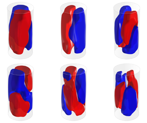
The third and fourth modes are represented in figure 8. Similarly to the first pair of POD modes, these modes share an almost identical pattern consisting of two counter-rotating large-scale rolls localized approximately in the same azimuthal plane. Such a pattern resembles considerably the DRS observed in cylindrical samples with aspect ratio lower than unity (Verzicco & Camussi Reference Verzicco and Camussi2003; Xia et al. Reference Xia, Sun and Cheung2008; Weiss & Ahlers Reference Weiss and Ahlers2011b), and also detected in specific snapshots of the present experiment (figure 4). Since both the pairs of modes 1–2 and 3–4 generally contribute to the structure of the instantaneous velocity fields, the emergence of the DRS is indeed associated with a weak correlation of the instantaneous velocity field with the first POD modes (i.e. small values of the projection of the snapshot onto these POD modes), as better shown later in § 5.3. When both the contributions from these POD mode pairs are not negligible, the SR and double-roll patterns are combined with each other. It is here observed that this can result in a torsion of the LSC. In order to show such a property, figure 9 reports the POD-based low-order reconstructions (LORs) of a selected snapshot by varying the number of modes employed. The LOR based only on the first two modes (figure 9a) is characterized by the presence of a quasi-planar LSC circulation: when the contribution from the second mode pair is added (figure 9b), the ascending and descending sides of the LSC appear to swirl around the vertical direction; the addition of the contributions from the remaining modes does not alter significantly this pattern, which in fact is present in the full snapshot (figure 9f). The above example seems to suggest a strict relationship between the torsional mode of the LSC (deeply investigated in the literature, e.g. Weiss & Ahlers (Reference Weiss and Ahlers2011b)) and the nature of the DRS. In principle, the DRS might be regarded as the result of an extreme torsion of the LSC.

Figure 8. Second pair of POD modes. Three-dimensional isosurfaces of the vertical velocity component corresponding to values of  $\pm 0.1$ of the maximum for (a) the third and (b) the fourth mode (red corresponds to the positive value) and (c) velocity vector map in the $xz$-plane for the fourth mode. The velocity magnitude is coded in the vector length, while the colour indicates the value of the vertical velocity (scaled by the maximum).
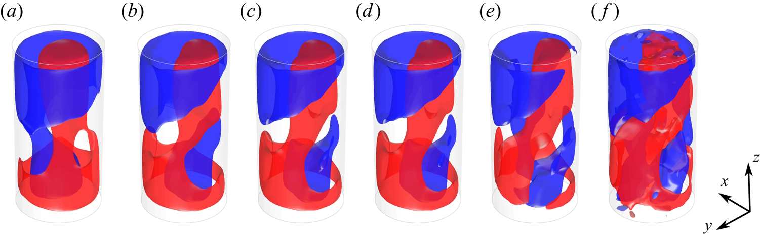
Figure 9. Torsion of the LSC due to the addition of the contribution from the third and the fourth POD mode. The POD based LOR of a specific snapshot by using the time-averaged velocity fields and the first (a) 2, (b) 4, (c) 6, (d) 8 or (e) 20 POD modes of the velocity fluctuation field and (f) instantaneous velocity field. Red and blue isosurfaces correspond to values of  $\pm 0.04w_0$.
It is also worth mentioning that the SR present in the first two POD modes is not a purely planar circulation, but has itself a swirled structure. This can be seen in figure 10(a), which reports the azimuthal profiles of the vertical velocity at three different heights, namely,  $0.25$, $0.5$ and $0.75$ of the cell height, for the second mode. Here, the data points indicate the experimental data (obtained by interpolation on an evenly spaced mesh), while the solid lines are the cosine fits to this data. The phase angles of these regression curves are clearly not coincident and the absolute difference between the phases of the curves related to the top and the bottom is approximately $15^{\circ }$. Furthermore, it can be noted that the profiles are slightly different from their cosine regressions, which suggests local flow velocity variations likely due to the presence of thermal plumes. Indeed, also the axially and radially averaged profiles reported in figure 7 are not optimally fitted by the cosine model. The above features (twisting of the SR and local flow velocity variations) are related to the fact that first POD modes, while capturing the most energetic coherent structures, are typically contaminated by smaller structures that exhibit a high degree of temporal correlation over the investigation time (Zhang, Liu & Wang Reference Zhang, Liu and Wang2014). Moreover, it should be remarked that, although in the literature the first-order azimuthal Fourier mode is generally associated with the LSC, there is no evidence for expecting that the LSC states (both the SRS and the DRS) have a purely harmonic structure. The observed deviation of the first two POD modes from a harmonic shape might be also associated with the oscillatory modes of the LSC which influence its instantaneous structure. For the purpose of comparison, in figure 10(b) the azimuthal profiles of the vertical velocity at the same heights and radial position are reported for the fourth mode. In such a case, the cosine fits of the profiles related to the top and the bottom are shifted by nearly $180^{\circ }$, whereas the profile at $z/H=0.5$ has a distribution very different from its cosine fit, since it corresponds to the flow region between the two rolls.

Figure 10. Azimuthal profiles of the vertical velocity at the heights  $z/H=0.25$ (red), $z/H=0.5$ (green) and $z/H=0.75$ (blue) and radial position $r/H=0.20$ for (a) the second POD mode and (b) the fourth POD mode. The data points represent the experimental measurements, whereas the solid lines are the cosine fits to this data. Values are scaled by the maximum of the vertical velocity component in each mode.
Figure 11 shows the morphology of the fifth and the sixth POD velocity mode. These two modes are characterized by the presence of four adjacent vertical currents localized in separate angular sectors of the cylindrical sample, as also visible from the slice of the velocity field at midheight (Figure 11c). When superimposed on the flow pattern given by mean flow field and the contributions from the first four POD modes, the contribution from this POD mode pair can result in an out-of-plane motion of the LSC, which squeezes it onto a side of the cylindrical cell. This is shown in figure 12 by means of the LORs of a specific snapshot by varying the number of modes employed. In the selected case, the addition of the contribution from the second pair of POD modes (compare figures 12a and 12b) does not change significantly the structure of the LSC, which lies approximately in the azimuthal plane  $x=y$. After the addition of the contributions related to the fifth and the sixth mode (figure 12c), the ascending and descending sides of the LSC are shifted in the direction normal to its plane and approach the sidewall on one side. The addition of two more POD modes (figure 12d) does not introduce significant changes, whereas the high-order POD modes (figure 12e,f) seem to modify the region of the flow opposite to the squeezed LSC. The case reported in figure 12 shows that the fifth and sixth modes are responsible of the sloshing mode of the LSC, that has been reported and investigated in numerous works (Brown & Ahlers Reference Brown and Ahlers2009; Xi et al. Reference Xi, Zhou, Zhou, Chan and Xia2009; Zhou et al. Reference Zhou, Xi, Zhou, Sun and Xia2009).
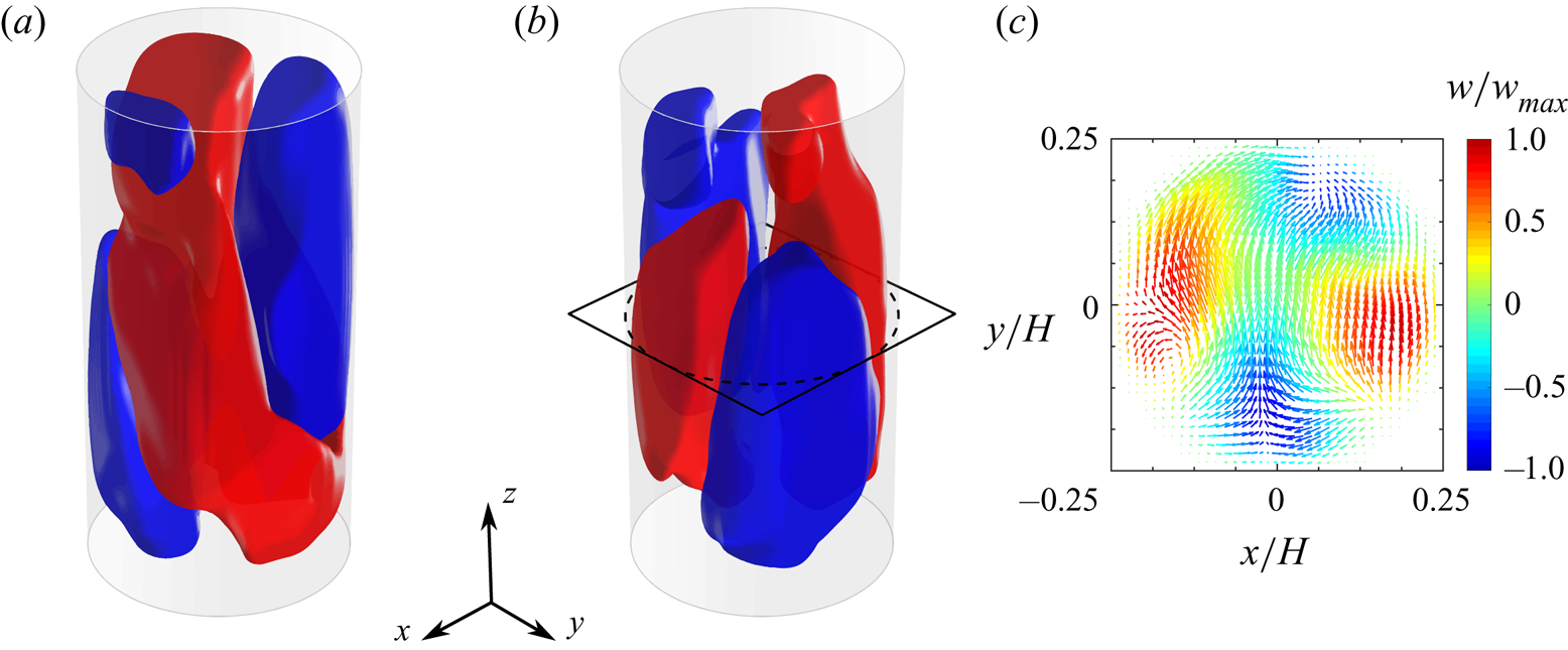
Figure 11. Third pair of POD modes. Three-dimensional isosurfaces of the vertical velocity component corresponding to values of  $\pm 0.1$ of the maximum for (a) the fifth and (b) the sixth mode (red corresponds to the positive value) and (c) velocity vector map in the $xy$-plane for the sixth mode. The velocity magnitude is coded in the vector length, while the colour indicates the value of the vertical velocity (scaled by the maximum).

Figure 12. Sloshing of the LSC due to the addition of the contribution from the fifth and sixth POD mode. POD based LOR of a specific snapshot by using the time-averaged velocity fields and the first (a) 2, (b) 4, (c) 6, (d) 8 or (e) 20 POD modes of the velocity fluctuation field and (f) instantaneous velocity field. Red and blue isosurfaces correspond to values of  $\pm 0.04w_0$.
5. Statistical analysis of the flow state
In this section the statistical behaviour of the LSC is analysed. In previous experimental investigations the LSC orientation and characteristic modes have been identified by measuring the azimuthal temperature distribution at the sidewall (Funfschilling et al. Reference Funfschilling, Brown, Nikolaenko and Ahlers2005; Brown & Ahlers Reference Brown and Ahlers2006b; Funfschilling et al. Reference Funfschilling, Brown and Ahlers2008; Xi & Xia Reference Xi and Xia2008; Weiss & Ahlers Reference Weiss and Ahlers2011b). Thermal probes are typically placed along circumferences at three different cell heights, namely  $z=0.25\,H$, $z=0.5\,H$ and $z=0.75\,H$, with a uniform angular spacing; the most common number of probes is eight. Since temperature measurements are not available in the present study, a similar analysis is carried out by focusing on the azimuthal profiles of the vertical velocity, as already done by Stevens et al. (Reference Stevens, Clercx and Lohse2011) in their numerical investigation. For this purpose, virtual anemometric probes are placed on circumferences at one quarter, one half and three quarters of the cell height localized at a radial distance of $0.9r_i$ from the cylinder axis ( $r_i=D/2$ is the cylinder internal radius). Since the present measurements are carried out in a relatively low $Ra$ regime, as suggested by Stevens et al. (Reference Stevens, Clercx and Lohse2011) it is necessary to employ a number of probes much larger than eight to have sufficient resolution to distinguish between the different states of the LSC. Therefore, 98 probes are placed with an angular spacing of approximately ${\rm \Delta} \varphi =3.7^{\circ }$ (linear spacing along the circumferences of approximately $2.11$ mm, i.e. $\approx 30$ voxels). The probe measurements are obtained by interpolating the Lagrangian trajectories as explained in § 2.3; since the resulting azimuthal profiles can be very noisy in the instantaneous velocity field, a moving time-averaging filter is used, as is suggested in Stevens et al. (Reference Stevens, Clercx and Lohse2011). As a final step, the discrete vertical velocity measurements $w_j^{(k)}$ are fitted to a cosine function according to the following model:
 \begin{equation} w_j^{(k)}=w_j+A_j\cos(\varphi^{(k)}-\varphi_j)+\varepsilon_j^{(k)},\end{equation}
where  $\varphi ^{(k)}=k{\rm \Delta} \varphi$ with $k=0,1,\ldots ,97$ are the angular positions of the probes, $w_{j}$, $A_j$ and $\varphi _j$ are the average velocity, the amplitude and the initial phase of the cosine fit at the $j$th height where measurements are taken and $\varepsilon _j^{(k)}$ is the residual error of the fit. The parameter $w_{j}$ is computed as the average of the available measurements $w_j^{(k)}$, while $A_j$ and $\varphi _j$ are estimated via a least-squares procedure by minimizing the sum of the squared residual errors $\sum _k (\varepsilon _j^{(k)})^{2}$. In the following, the indices $b$,
$b$,  $m$ and $t$ are used in place of the index $j$ to denote the quantities related to the heights $z=0.25\,H$ (bottom), $z=0.5\,H$ (middle) and $z=0.75\,H$ (top), respectively. In the literature, the LSC orientation is identified by the angle $\varphi _m$, while the differences between each pair of the angles $\varphi _b$, $\varphi _m$ and $\varphi _t$ provide insight into the current state of the LSC.
In addition to the above analysis, following Stevens et al. (Reference Stevens, Clercx and Lohse2011), the time-resolved relative LSC strength  $S_j$ at the generic height is also calculated as the ratio of the energy $\tilde {E}_j^{(1)}(t)$ in the first Fourier mode of the azimuthal vertical velocity profile to the total energy in all Fourier modes, according to the following equation:
 \begin{equation} S_j(t) = \left.\left( \frac{ \tilde{E}_j^{(1)}(t) }{\displaystyle \sum_{i=1}^{N} \tilde{E}_j^{(i)}(t) } -\frac{1}{N} \right) \right/ \left( 1 - \frac{1}{N} \right),\end{equation}
where  $N$ is the number of the available Fourier modes. A value of $S_j$ greater than 0.5 indicates a high goodness of the cosine fit, which is a necessary condition for the occurrence of the LSC, according to Stevens et al. (Reference Stevens, Clercx and Lohse2011). Alternatively, the strength of the LSC can be assessed based on the vertical velocity amplitudes $A_j$. According to Weiss & Ahlers (Reference Weiss and Ahlers2011b), the existence of the LSC in the SRS or the DRS implies that $A_b$, $A_m$ and $A_t$ have to be higher than a fixed threshold, otherwise a transitional state (TS) of the turbulent convection is observed. Weiss & Ahlers (Reference Weiss and Ahlers2011b) fixed as a reasonable threshold $15\,\%$ of the time-averaged amplitude $\overline {A_j}$ and defined as ‘events’ all the realizations in which one of the three amplitudes is lower than such a threshold. In particular, the simultaneous drop of all the amplitudes below the threshold is associated with a cessation of the LSC.
In the following, an analysis of the flow behaviour based on the cosine fits of the vertical velocity profile is carried out for the purpose of comparison with the results existing in the literature. In § 5.2, the identification of the SRS and the DRS is performed using the criteria introduced by Xi & Xia (Reference Xi and Xia2008) and Weiss & Ahlers (Reference Weiss and Ahlers2011b). Based on the latter, the LSC is in the SRS when the three amplitudes  $A_j$ are simultaneously above the thresholds $0.15\,\overline {A_j}$ (i.e. the current state is not an event) and the phase differences $|\delta \varphi _{ij}|=|\varphi _i-\varphi _j|$ for each $i\neq j$ are lower than $60^{\circ }$. On the other side, the occurrence of the DRS requires $|\delta \varphi _{tb}|>120^{\circ }$ and the amplitudes of the top and the bottom vertical velocity profiles to be above their thresholds. All the remaining states are identified as TSs. In § 5.3, the relationship between the SRSs and DRSs identified with the above criteria and the POD modes is investigated and the limitations of such an approach are shown. Contextually, a more robust method based on the POD analysis is introduced.
5.1. Statistical behaviour of the LSC strength
Figure 13 reports the probability density functions (p.d.f.s) and the cumulative distribution functions (c.d.f.s) of the amplitudes  $A_j$ for the top, middle and the bottom. With the chosen scaling ( $A_j$ normalized by its time-averaged value $\overline {A_j}$), the three p.d.f.s essentially collapse on each other, as already observed in the study of Weiss & Ahlers (Reference Weiss and Ahlers2011b) for $Ra=9\times 10^{10}$, $Pr=4.38$ and $\varGamma =0.5$. However, differently from the latter investigation, in the present case the maximum of the p.d.f. is reached at a value lower than unity for the middle and the top, whereas it is found at $A_j=\overline {A_j}$ for the bottom. In figure 13(b) the dashed line represents the threshold indicated by Weiss & Ahlers (Reference Weiss and Ahlers2011b) to identify an event. The probability that $A_j<0.15\overline {A_j}$ is $3.15\,\%$, $1.73\,\%$ and $2.98\,\%$ for the bottom, middle and top, respectively. These values correspond to frequencies of such events that are, respectively, equal to $112\tau _\nu ^{-1}$, $53\tau _\nu ^{-1}$ and $106\tau _\nu ^{-1}$, with $\tau _\nu =H^{2}/\nu$ being the viscous time. Such values are in agreement with the observations of Xi & Xia (Reference Xi and Xia2007) and Weiss & Ahlers (Reference Weiss and Ahlers2011b) for higher Rayleigh numbers ( $>10^{9}$) and lower Prandtl number ( $\approx 4.3$). However, a remarkable difference of the present experiment from the latter studies is that the occurrence frequency of the events at midheight is found to be significantly lower than (almost one half) those at the bottom and the top. Moreover, no cessations (i.e. events when all the three amplitudes are below their thresholds) are observed in the present investigation. This is consistent with the experimental observations of Weiss & Ahlers (Reference Weiss and Ahlers2011b), who found a frequency of occurrence of cessations equal to $1.1\tau _\nu ^{-1}$, which turns into a value of approximately 0.2 cessations per hour in the present case, although in disagreement with the study of Xi & Xia (Reference Xi and Xia2007), which reported a considerably higher frequency of cessations in analogous operating conditions (i.e. $Ra$ in the range $10^{10}$– $10^{11}$ and $Pr$ between $4.38$ and $5$).
$5$).

Figure 13. Probability distribution of the vertical velocity amplitudes of the LSC at the bottom ( $z/H=0.25$), middle ( $z/H=0.5$) and top ( $z/H=0.75$): (a) p.d.f.; (b) c.d.f.. Each amplitude is normalized by the corresponding time-averaged value.
The statistical distributions of the LSC strengths  $S_j$ are reported in figure 14. The behaviour of $S_m$ (black dots) is similar to that reported in the numerical study of Stevens et al. (Reference Stevens, Clercx and Lohse2011) for analogous operating conditions (but with a perfect adiabatic wall condition). Here $S_m$ can be considered as representative of the strength of the LSC in the SRS, while $S_t$ (blue triangles) and $S_b$ (red triangles) are related to both the SRS and the DRS. Indeed, the higher values of the $S_m$ p.d.f. compared with the p.d.f.s of $S_b$ and $S_t$ over the range $0< S_j<0.2$ are essentially related to the occurrence of the DRS which causes $S_m$ to have values statistically smaller than those of $S_t$ and $S_b$. It is also noted that $S_b$ shows values of the p.d.f. greater than those related to $S_t$ in the range $0< S_j<0.05$. This indicates that in the SRS the strength of the LSC in the top half of the cell is statistically greater than that in the bottom half. Such an observation is corroborated by figure 14(b), where it is apparent that the c.d.f. of $S_t$ has lower values than those of $S_m$ and $S_b$. The reason for this behaviour can be found in the influence of the temperature condition at the external side of the sidewall: as aforementioned, hot plumes rising from the bottom are subjected to a stronger heat transfer with the sidewall than the cold plumes and this results in a weakening of the recirculation in the lower half of the cell.

Figure 14. Probability distribution of the LSC strength at the bottom ( $z/H=0.25$), middle ( $z/H=0.5$) and top ( $z/H=0.75$) of the cell: (a) p.d.f.; (b) c.d.f..
5.2. Statistical occurrence and properties of the SRS and DRS
As commented above, the statistical distribution of the absolute differences  $|\delta \varphi _{ij}|$ provides insight in the occurrence of the SRS and the DRS. Figure 15 reports the p.d.f.s of the absolute differences $|\delta \varphi _{tm}|$ (blue triangles), $|\delta \varphi _{bm}|$ (red triangles) and $|\delta \varphi _{tb}|$ (black squares). Such a diagram is obtained using only the samples that satisfy the criterion for the LSC amplitude ( $A_j>0.15\overline {A_j}$). The distributions of $|\delta \varphi _{tm}|$ and $|\delta \varphi _{bm}|$ are similar and they exhibit a bell-like shape. This is in very good agreement with the experimental results of Weiss & Ahlers (Reference Weiss and Ahlers2011b) and the numerical results of Stevens et al. (Reference Stevens, Clercx and Lohse2011). On the other side, $|\delta \varphi _{tb}|$ shows higher values of the p.d.f. between $0^{\circ }$ and $60^{\circ }$ and lower values between $120^{\circ }$ and $180^{\circ }$. This suggests that the probability of occurrence of the DRS is slightly lower than that of the SRS. Indeed, the computed values of such probabilities are $27\,\%$ and $29\,\%$, respectively, for the DRS and the SRS; on the other hand, the TSs have a probability of occurrence of $44\,\%$ among states that are not classified as events. Such results are in agreement with the much longer experiments of Weiss & Ahlers (Reference Weiss and Ahlers2011b), who observed that, for $Ra=2\times 10^{8}$ and $Pr=4.38$, the flow state is undefined for approximately $50\,\%$ of the time (in this regard, it is remarked that the events cover only $6\,\%$ of the total time in the present experiments, thus the TSs constitute $41\,\%$ of the total duration).

Figure 15. Probability distributions for the absolute differences between the orientation of the LSC at the bottom ( $z/H=0.25$), middle ( $z/H=0.5$) and top ( $z/H=0.75$). Only the samples satisfying the criterion for the amplitudes have been considered (see the text for explanation). When exceeding $180^{\circ }$, the difference $|\delta \varphi _{ij}|$ was replaced by $360^{\circ }-|\delta \varphi _{ij}|$. The dashed lines indicate the thresholds for the identification of the SRS ( $|\delta \varphi _{ij}|<60^{\circ }$ for any $i\neq j$) and the DRS ( $|\delta \varphi _{tb}|>120^{\circ }$) according to Xi & Xia (Reference Xi and Xia2008) and Weiss & Ahlers (Reference Weiss and Ahlers2011b).
Figure 16 shows the p.d.f.s of the LSC orientations at the top, middle and bottom for both the SRS and the DRS. The p.d.f.s for the SRS (figure 16a) are essentially the same at all the three levels and they exhibit a pronounced peak around  $\varphi =0^{\circ }$, while the p.d.f.s go to zero towards $\pm 180^{\circ }$. The existence of a preferential orientation of the LSC has already been noted in previous works. Brown & Ahlers (Reference Brown and Ahlers2006a) demonstrated that symmetry-breaking inhomogeneities can be generated by several factors, among which are the Earth's Coriolis force and imperfections of the experimental apparatus such as a slight tilt of the sample, small horizontal thermal gradients in the top and bottom plates and eccentricity of the circular cross-section. However, the studies of Xi & Xia (Reference Xi and Xia2008) and Weiss & Ahlers (Reference Weiss and Ahlers2011b) have shown that the effect of the Earth's Coriolis force seems to be smaller in convection cells with $\varGamma =0.5$ than those with $\varGamma =1$. Interestingly, the p.d.f.s of the LSC orientations for the DRS (figure 16b) are fairly uniform for the top and the bottom, whereas lower values around $\pm 180^{\circ }$ are found for the middle. In conclusion, it is possible to assert that a preferential orientation does not exist for the DRS.

Figure 16. Probability distributions for the LSC orientation at the bottom ( $z/H=0.25$), middle ( $z/H=0.5$) and top ( $z/H=0.75$) for (a) the SRS and (b) the DRS.
Figure 17 reports the p.d.f. of the LSC angular velocity estimated as the time derivative of the LSC orientation at midheight  $\varphi _m$. The p.d.f. computed using all the available samples (blue dots) has a Gaussian shape in the central part with fairly heavy tails, in agreement with the results from the previous investigations of Xi & Xia (Reference Xi and Xia2008) and Weiss & Ahlers (Reference Weiss and Ahlers2011b). In the same diagram, the p.d.f. for the samples satisfying the criterion of Stevens et al. for identification of a coherent LSC based on circulation strength, i.e. $S_m>0.5$, (black squares) and the p.d.f. for the samples with $A_m>\overline {A_m}$ (red diamonds) are also reported. Such curves exhibit an almost identical narrower Gaussian shape, which indicates that the high values of the angular velocity of the LSC are indeed related to states of the turbulent convection with a not-well defined LSC, in which the determination of the LSC orientation is affected by greater uncertainty.

Figure 17. Probability distribution for the angular velocity of the LSC. The light-blue solid line is the Gaussian fit to the data related to all samples in the range between  $\pm 0.05$ rad s $^{-1}$.
5.3. Relationship of the SRS and the DRS with low-order POD modes
In this section, the relationship of the SRS and the DRS with the first two pairs of POD modes is investigated by focusing on the statistical behaviour of the corresponding POD coefficients, which are the projections of the snapshots onto the POD modes. Since the first POD modes appear to be paired as shown above, it is convenient to define an energy contribution related to a single pair of the POD modes and study the statistical distribution of this quantity. In the following, the energy contribution due to the pair of the  $i$th and the $j$th POD mode is denoted with the symbol $E^{(i-j)}$.
Figure 18 reports the c.d.f.s of the energy contributions  $E^{(1-2)}$ and $E^{(3-4)}$ distinguishing between the samples in the SRS, in the DRS and in a TS. It is worth remarking that a high value of the c.d.f. corresponding to a certain energy level $E^{*}$ means that the probability that $E^{(i-j)}< E^{*}$ is high. Consequently, figure 18(a) shows that the first pair of POD modes statistically contributes more to the SRS than to the DRS. On the other side, figure 18(b) shows that the second pair of POD modes statistically contributes more to the DRS than to the SRS. It is also noted that the energetic contributions of the POD modes’ pairs to the TSs are on an intermediate level between those related to the SRS and the DRS.

Figure 18. Cumulative probability distributions of the energy contribution due to the (a) the first pair and (b) the second pair of POD modes for the different states of the LSC. Energies are scaled by the maximum value detected over the entire measurement duration.
Another useful perspective on the relationship between the states of the LSC and the POD modes is obtained by representing the c.d.f.s of the energies  $E^{(i-j)}$ of the different POD mode pairs for all the samples corresponding to a single state of the LSC. Such a representation is given in figure 19 for the SRS and the DRS; here, energy values are scaled by the mean energy $\overline {E}^{(1-2)}$ contained in the first pair of POD mode in the corresponding state of the LSC. Figure 19(a) shows that the contribution of the first pair of POD modes to the SRS is statistically preponderant with respect to the contributions of the remaining modes. This could seem an obvious consideration since the POD modes retain most of the time-averaged fluctuating kinetic energy. However, it should be remarked that the c.d.f.s in figure 19(a) were constructed by using only the samples in the SRS and not the whole ensemble. When a subset of samples is considered, it is not true in general that the first two POD modes contain the greatest amount of kinetic energy. Indeed, in figure 19(b) it is possible to note that the largest energy contribution to the snapshots in the DRS is provided by the third and the fourth mode.

Figure 19. Cumulative probability distributions of the mode pair energies for (a) the SRS and (b) the DRS. Energies are scaled by the average energy in the first pair of POD modes related to each state.
The above analysis suggests that the occurrence of the SRS is related to the dominance of the energy contribution from the first two POD modes over the remaining modes, as well as the appearance of the DRS in the unsteady evolution is associated with the energetic prevalence of the third and the fourth POD modes. In order to better show this property and also to discuss the limits of the criteria for the identification of the LSC states used up to this point, in the following focus is given to the unsteady flow evolution over specific time intervals of the experiment.
Figure 20 reports a time sequence related to a transition from the DRS to the SRS. In figure 20(a) the time behaviour of the energy contributions from the POD modes to the total kinetic energy of the fluctuating velocity field is represented, whereas figure 20(b–g) show the 3-D structure of the first-order azimuthal Fourier modes of the instantaneous vertical velocity field corresponding to the time instants marked with yellow lines in figure 20(a). It is worth remarking that the first-order azimuthal Fourier mode is indeed the harmonic regression (with zero mean) of the velocity signal along the azimuthal direction. Therefore, such a mode reflects the current state of the LSC, provided that its energy is larger enough than the higher-order azimuthal modes. Based on the approach of Stevens et al. (Reference Stevens, Clercx and Lohse2011), the relative strength of the first-order azimuthal Fourier mode is evaluated using the following definition:
 \begin{equation} S(t) = \left.\left( \frac{ \tilde{E}^{(1)}(t) }{\displaystyle \sum_{i=1}^{N} \tilde{E}^{(i)}(t) } -\frac{1}{N} \right) \right/ \left( 1 - \frac{1}{N} \right).\end{equation}
Equation (5.3) is analogous to (5.2), except that here  $\tilde {E}^{(1)}(t)$ and $\sum _{i=1}^{N} \tilde {E}^{(i)}(t)$, respectively, define the energy in the first-order Fourier mode and the sum of the energies in all Fourier modes of the 3-D velocity field (not only of the vertical component). In figure 20(a) the behaviour of $S(t)$ is also reported (pink curve). It is worth remarking that, according to Stevens et al. (Reference Stevens, Clercx and Lohse2011), $S(t)>0.5$ indicates a secondary effect of the plumes and/or corner flows on the coherence of the LSC (the first Fourier modes contains at least $50\,\%$ of the energy of the velocity field). With regard to the time sequence of figure 20, $S(t)$ is always above this threshold, thus the flow is organized in a well-defined LSC.

Figure 20. A time sequence illustrating the transition from the DRS to the SRS. (a) Evolution of the contributions from the POD modes to the total kinetic energy of the flow and of the strength  $S$ of the first-order azimuthal Fourier mode of the 3-D velocity field. (b–g) First-order azimuthal Fourier mode of the vertical velocity field at the time instants marked by the yellow vertical lines in panel (a): isosurfaces of the vertical velocity corresponding to the values $\pm 0.01w_0$ (red corresponds to the positive value).
In figure 20(a) the time is normalized by the free-fall time  $\tau _0=H/w_0$ (which is approximately $3.87$ s in the present case). A different time scale is also reported based on the convective time $\tau _c=D/u_c$ with $u_c$ being the root mean square of the horizontal velocity over the time and the cell volume. In the literature, the large-scale eddy turnover time is usually estimated from the vertical velocity (e.g. see Bailon-Cuba et al. Reference Bailon-Cuba, Emran and Schumacher2010). The present choice of using the horizontal velocity is motivated by the observation that the dynamics of some LSC oscillatory modes, such as the torsional and the sloshing mode, is characterized by times faster than the LSC turnover time $\tau _{{LSC}}$, and such times depend on the horizontal motions in the cell. An estimate of $\tau _{{LSC}}$ is given by $\tau _{{LSC}}=H/w_c$ with $w_c$ being the root mean square of the vertical velocity over the time and the cell volume. In the present experiments $\tau _{{LSC}}\approx 3\tau _c\approx 52\tau _0$.
Focusing on the behaviour of the energy in the POD modes, from figure 20(a) it is apparent that the energy in the POD modes 3–4, after an initial increase, monotonically decreases across the DRS phase of the flow evolution and reaches a minimum in the TS phase. Conversely, the energy contribution from the POD modes 1–2, despite some fluctuations, undergoes a continual increase up to a maximum at the beginning of the SRS phase. The energy in the POD modes 5–6 reaches relevant values at the turn of the DRS phase and vanishes in the TS one. At the beginning of the sequence (time instant (b)) the prominent value of the energy in the POD modes 3–4 results in a well-defined planar double-roll structure of the flow (the two counter-rotating rolls lie in the same plane), as visible in figure 20(b). The weakening of the contribution from the POD modes 3–4 and the gradual strengthening of that from the POD modes 1–2 during the DRS phase is accompanied by a rotation of the roll in the lower half of the cell. A significant misalignment of the two rolls is, however, observed only after the energy in the POD modes 1–2 has reached a value equal to half of the energy in the POD modes 3–4 (time instant (d), see figure 20c,d). In the TS phase, the flow is much more organized in a twisted domain-filling circulation, as can be inferred from 20(f). It is interesting to note that at the time instant (f), despite the energies in the POD mode pairs 3–4 and 5–6 are in fact insignificant compared with the energy in the POD modes 1–2, the LSC does not have a planar structure. This can be associated with the non-negligible value of the energy in the higher-order modes. Finally, a planar SR structure is attained in the SRS phase when the energy in the POD modes 1–2 is dominant. In conclusion, the above example, on one side, confirms that the occurrence of the SRS and of the DRS is related to the energetic prevalence of the associated POD mode pairs, on the other side, it suggests that a possible mechanism of the transition between the DRS to the SRS is the torsional mode of the LSC.
A distinct time sequence is reported in figure 21. In this case, the flow evolves through an alternation of DRSs and TSs, identified via the criteria introduced above and based on the comparative analysis of the azimuthal velocity profiles at three different heights. The coherence of the LSC, indicated by the value of  $S$, is lower than the previous case; however, for most of the time, $S(t)$ is around $0.5$, thus the structure of the first-order azimuthal Fourier mode (figure 21b–g) still provides a reliable description of the flow morphology. Interestingly, the diagram in figure 21 shows that, except in the beginning and in the final part of the selected time interval, the energy in the POD modes 3–4 is considerably smaller than the energies in the POD modes 1–2 and 5–6. Indeed, a well-defined DRS is only detectable in these two phases of the evolution (see figures 21b and 21g). At the other stages (figure 21c–f) the flow tends to organize itself in an SRS, although the LSC does not exhibit an exactly planar structure at any time; indeed, it has a twisted shape (this is associated with the contribution from the POD modes 5–6, which is comparable to that of the POD modes 1–2). It is, therefore, clear that the adopted criteria for the detection of the LSC state are imprecise in the present case. In particular, focusing on the time instant (d), the flow state is classified as DRS based on such criteria, however, an LSC in the SRS is detected both in the first-order azimuthal Fourier mode in figure 21(d) and in the full instantaneous velocity field, which is represented in figure 22. Here, both the isosurfaces (figure 22a) and the $yz$-slice (figure 22b) of the vertical velocity field show the presence of an LSC in an SRS. Stevens et al. (Reference Stevens, Clercx and Lohse2011) noticed that the misinterpretation of the state of the large-scale flow assessed using a cosine fit procedure on the temperature or the velocity profiles can be associated with passing plumes and/or the corner flows: the lower the Rayleigh number and the cell aspect ratio, the more relevant such an issue. Figure 22(c) reports the azimuthal profiles of the vertical velocity at the heights $z/H=0.25,0.5,0.75$ and radial position $r/r_i=0.9$, which have been used in the present case for the determination of the LSC orientation. The diagram clearly shows the low correlation of the cosine fits for the considered profiles; indeed, the corresponding strengths are $S_b=0.11$, $S_m=0.01$ and $S_t=0.11$. Therefore, following the approach of Stevens et al. (Reference Stevens, Clercx and Lohse2011), one might conclude that the state of the LSC is not defined at the selected time instant. Nevertheless, such a misinterpretation is purely related to the choice of the velocity probes employed in the present case. To better show this, in figure 22(d) the azimuthal vertical velocity profiles for the radial location $r/r_i=0.4$ at the bottom, the middle and the top are reported. In this case, the cosine fits show a high goodness; the corresponding strengths are $S_b=0.50$, $S_m=0.81$ and $S_t=0.81$.
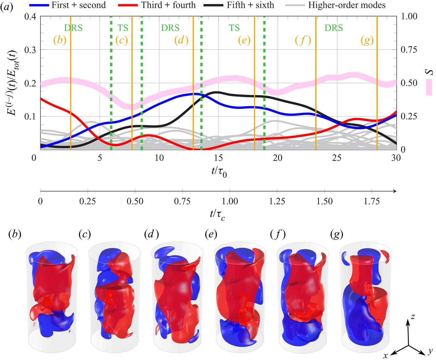
Figure 21. A time sequence illustrating an alternation between the DRS and the TS. (a) Evolution of the contributions from the POD modes to the total kinetic energy of the flow and of the strength  $S$ of the first-order azimuthal Fourier mode of the 3-D velocity field. (b–g) First-order azimuthal Fourier mode of the vertical velocity field at the time instants marked by the yellow vertical lines in panel (a): isosurfaces of the vertical velocity corresponding to the values $\pm 0.01w_0$ (red corresponds to the positive value).

Figure 22. Snapshot of the velocity at the time instant (d) of figure 21: (a) isosurfaces of vertical velocity corresponding to the values  $\pm 0.02 w_0$ (red and blue surfaces for the positive and the negative value, respectively); (b) velocity vector map in the $yz$-plane, the velocity magnitude is coded in the vector length, while the colour indicates the value of the vertical velocity (scaled by the free-fall velocity $w_0$); (c,d) azimuthal profiles of the vertical velocity at the heights $z/H=0.25$ (red), $z/H=0.5$ (green) and $z/H=0.75$ (blue) for radial positions (c) $r/r_i=0.9$ and (d) $r/r_i=0.4$. The data points represent the experimental measurements, whereas the solid lines are the cosine fits based on this data.
The above analysis reveals the limitations of the criteria for the identification of the LSC state classically used in the literature. On the other side, the POD analysis appears as a powerful tool for the characterization of the flow state and more reliable criteria can be formulated on such a basis. It is evident that a well-defined LSC (in either the SRS or the DRS) results from the energetic prevalence of the first two pairs of POD modes. Thus, after denoting the energy contribution from these modes as  $E^{(1-4)}(t)$, a first requirement for the occurrence of a definite LSC is that $E^{(1-4)}(t)/E_{{tot}}(t)>\varepsilon _{{LSC}}$, where $E_{{tot}}(t)=\sum _i E^{(i)}(t)$ is the total energy in the POD modes (equal to the energy of the instantaneous fluctuating velocity field) and $\varepsilon _{{LSC}}$ is a fixed threshold. On the other side, the occurrence of the SRS or the DRS is related to the relative importance of the energy in the POD mode pairs 1–2 and 3–4, i.e. on the ratio $E^{(3-4)}(t)/E^{(1-2)}(t)$. It is then convenient to define two further thresholds: $\varepsilon _{{SRS}}$ such that the SRS occurs when $E^{(3-4)}(t)/E^{(1-2)}(t)<\varepsilon _{{SRS}}$ and $\varepsilon _{{DRS}}$ such that the DRS occurs when $E^{(3-4)}(t)/E^{(1-2)}(t)>\varepsilon _{{DRS}}$. The TSs are classified as those realizations at any time $t$ such that $\varepsilon _{{SRS}}< E^{(3-4)}(t)/E^{(1-2)}(t)<\varepsilon _{{DRS}}$. Obviously, the above thresholds should be defined in such a way that $0<\varepsilon _{{LSC}}<1$, $0<\varepsilon _{{SRS}}<1$ and $\varepsilon _{{DRS}}>1$.
Figure 23 reports the p.d.f.s of both the quantities  $E^{(1-4)}/E_{{tot}}$ and $E^{(3-4)}/E^{(1-2)}$. The p.d.f. of $E^{(1-4)}/E_{{tot}}$ (figure 23a) has a quasi-Gaussian shape with a peak around $0.19$ which is indeed approximately equal to the sum of the percentage energy levels of the first four POD modes ( $\approx 21\,\%$), already reported in § 4. In figure 23(a) a threshold value $\varepsilon _{{LSC}}$ is also reported. This has been assumed equal to the sum of the percentage energy levels of the POD modes 3–4, which is $\approx 8.4\,\%$. Although arbitrary, such a choice is based on the idea that, when the energy contribution from the POD modes 1–2 is negligible, the occurrence of the DRS requires the instantaneous contribution from the POD modes 3–4 to be greater than its averaged value. With this threshold, the probability of occurrence of a well-defined LSC is estimated to be $89\,\%$, thus the probability of an event is $11\,\%$. In figure 23(b) the p.d.f. of $E^{(3-4)}/E^{(1-2)}$ is built by considering only the samples where a well-defined LSC is detected (i.e. such that $E^{(1-4)}/E_{{tot}}>\varepsilon _{{LSC}}=8.4\,\%$). It is possible to see that this p.d.f. is monotonically decreasing and the probability that $E^{(3-4)}\gg E^{(1-2)}$ is small. The thresholds values $\varepsilon _{{SRS}}$ and $\varepsilon _{{DRS}}$ are also denoted in the same figure with dashed lines. In particular, $\varepsilon _{{SRS}}$ has been chosen equal to the statistically average value of the quantity $E^{(3-4)}/E^{(1-2)}$, whereas $\varepsilon _{{DRS}}=1+(1-\varepsilon _{{SRS}})$; the resulting values are $\varepsilon _{{SRS}}=0.67$ and $\varepsilon _{{DRS}}=1.33$. With these thresholds, the probability of occurrence for the SRS, the TS and the DRS are, respectively, $49\,\%$, $18\,\%$ and $33\,\%$, among states that are not classified as events. Therefore, compared with the values determined with the criteria classically used in the literature ( $29\,\%$, $44\,\%$ and $27\,\%$, respectively, for the SRS, the TS and the DRS), a greater frequency of occurrence of the SRS and lower frequency of occurrence of the TS are found, whereas the frequency of occurrence of the DRS is substantially unchanged. This suggests that the criteria adopted in the literature lead essentially to a misinterpretation of the flow state in the SRS, which is often classified erroneously as a TS.
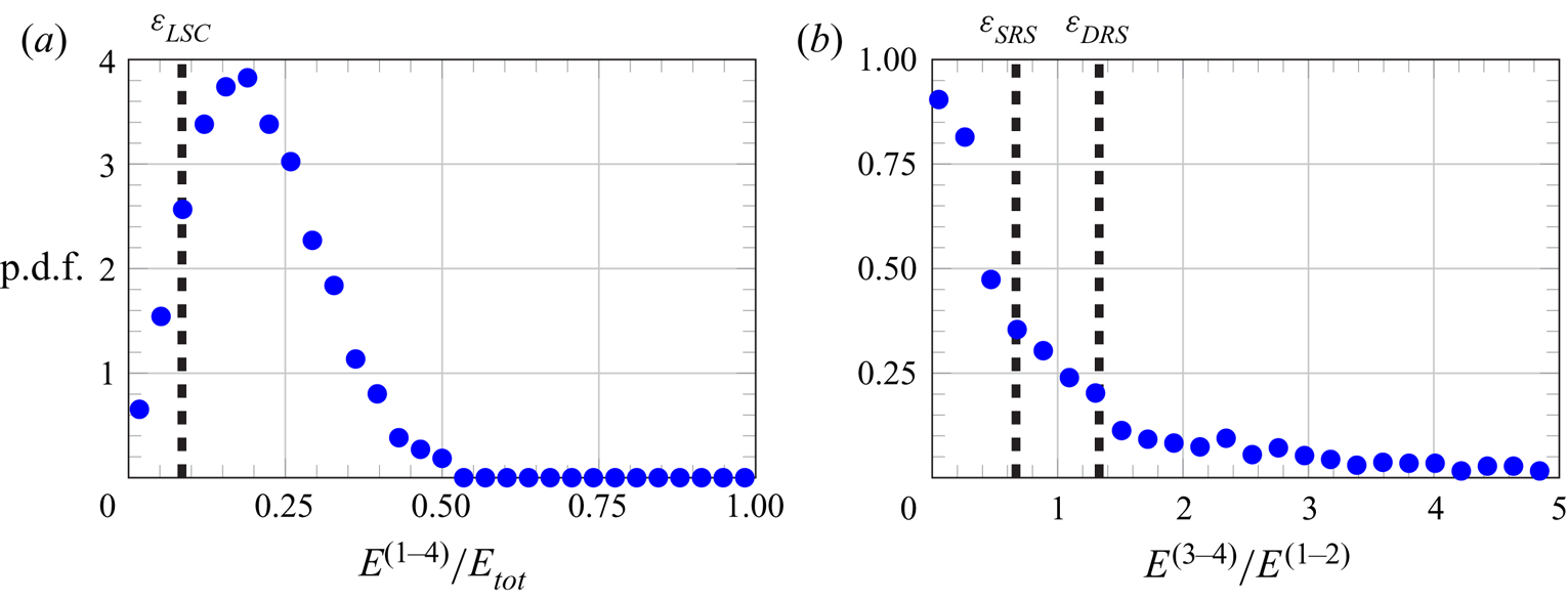
Figure 23. Criteria for the identification of the flow state based on POD analysis of the velocity field. (a) P.d.f. of the ratio of the energy in the first four POD modes to the total energy of the fluctuating velocity field. The dashed line indicates the threshold for the identification of a well-defined LSC. (b) P.d.f. of the ratio of the energy in the POD modes 3–4 to the that in the POD modes 1–2. The dashed lines indicate the threshold for the identification of the SRS and the DRS.
The evidence that the first two POD modes contribute more to the SRS allows us to conceive a different way of detecting the LSC orientation, based on the correlation of the snapshots with the first two POD modes. Such a technique and its relationship with the method adopted above is discussed in the next section.
5.4. Identification of LSC orientation based on POD
In this section, an alternative method of detecting the LSC orientation is introduced. Such a method relies on an LOR of snapshots based on only the first two POD modes, which, as aforementioned, contribute more to the SRS. In principle, the following steps have to be performed: reconstructing each snapshot by combining the mean velocity field and the contributions from the first two POD modes; extracting the azimuthal profile of the vertical velocity at midheight; estimating the parameters of the cosine fit model and thus the LSC orientation  $\varphi _m$. The main advantage of this method is that the contributions of secondary modes, such as torsion and sloshing, are filtered out by the LOR process, since they are related to the higher-order POD modes. To ease computation, in the second step, it is possible to extract the azimuthal profiles of the vertical velocity at midheight for the first and the second mode and combining them with the corresponding POD mode temporal coefficients to obtain the velocity profile for a selected snapshot. A more robust procedure consists in combining the profiles reported in figure 7, i.e. the azimuthal profiles of the axially and radially averaged velocity for the first and the second mode. This is more accurate since, as shown in § 4, the SR in the first two POD modes has a twisted structure.
Figure 24(a) presents the p.d.f. of the LSC orientation based on the method described above (denoted by the symbol  $\varPhi$). Differently from the p.d.f. of $\varphi _m$ (figure 16a), the p.d.f. of $\varPhi$ does not feature a well-defined Gaussian distribution. However, a preferred orientation is still detected, approximately at $\varPhi \approx -12^{\circ }$. This indeed corresponds to the phase angle of the blue curve in figure 7. Such a result is expected since the first POD mode should in principle capture a preferential orientation of the LSC, if any. The fact that the method based on the cosine fit of the azimuthal velocity profile at midheight does not present a prominent peak at the LSC orientation of the first POD mode could indicate a bias in the estimation of the LSC orientation. Indeed, when the p.d.f. of the difference between $\varPhi$ and $\varphi _m$ is plotted (blue dots in figure 24b), a peak at the above-mentioned angle is not observed. However, when restricting to only the samples related to the SRS, a peak appears in the p.d.f. The origin of such a bias is not clear and further investigations are needed on this point.

Figure 24. Statistical behaviour of the LSC orientation identified by means of the first two POD modes: (a) p.d.f.; (b) comparison with the LSC orientation identified by the cosine fit of the azimuthal velocity profile at  $z/H=0.5$. The SRS is identified with criteria based on the analysis of the vertical velocity azimuthal profile.
6. Conclusions
This work has investigated the statistical behaviour and the characteristic modes of RB convection inside a cylinder with aspect ratio equal to one half at specific flow conditions, namely Rayleigh and Prandtl numbers equal to  $1.86\times 10^{8}$ and $7.6$ (the working fluid is water). A peculiarity of the present experiment is that the convection cell has a smaller size than systems that have been investigated previously in the literature, and this allows velocimetry measurements in the whole interior of the convection cell. In such a way, it has been possible to extract the full 3-D structure of the flow modes. Proper orthogonal decomposition of the fluctuating velocity field has been used for such a purpose. The structure of the POD modes reflects and gives a clear picture of the most characteristic patterns in which the LSC organizes itself in the instantaneous evolution. The SRS and the DRS have been recognized in the first POD modes; the latter appear to be coupled in pairs since any azimuthal orientation of the flow pattern is possible in the unsteady evolution. Additionally, it has been shown that states of the LSC different from a pure SRS or DRS, which are typically associated with the LSC oscillatory modes (such as torsion and sloshing), are retrieved from the combination of the velocity field components related to distinct POD mode pairs. This proves that the oscillatory modes are ascribable to the dynamic evolution of the contributions from the POD velocity modes. A clear picture of such mechanisms has been drawn by means of low-order reconstruction of specific snapshots. To the authors’ knowledge, this is the first attempt to concretely visualize the LSC oscillatory modes in the whole convection cell, which in previous studies have been inferred and statistically analysed from the azimuthal measurements of the temperature at the sidewall or two-dimensional velocimetry measurements.
In order to study the relationship between the occurrence of the SRS and the DRS in the unsteady evolution and the energetic prevalence of the related POD modes, the statistical behaviour of the LSC has been characterized with conventional diagnostic methods based on the analysis of the azimuthal profiles of the vertical velocity near the cylinder sidewall at three different heights, i.e.  $z/H=0.25$, $z/H=0.5$ and $z/H=0.75$. Results consistent with the existing literature on the topic have been retrieved regarding the statistical analysis of both the LSC strengths at the different heights and the LSC azimuthal orientation. Moreover, it has been observed that the detection of the SRS is strictly correlated to the energetic dominance of the POD modes 1–2, while the occurrence of the DRS is associated with the prevalence of the POD modes 3–4. Nevertheless, specific time sequences have been found, in which the criteria based on the cosine fits of the azimuthal velocity profiles fail in the detection of the LSC state. Previous works (Stevens et al. Reference Stevens, Clercx and Lohse2011) have correctly identified the reason for this failure in the passage of plumes and/or corner flows across the locations of the probes for the measurement of the temperature or the vertical velocity. The present study has shown that the bulk flow can exhibit a distinct organization from the variety of plumes localized in the proximity of the sidewall. Such a complex flow structure can lead to misinterpretation of the actual large-scale flow state inferred from the azimuthal measurements at the bottom, middle and top of the cell in the proximity of the sidewall. In the light of these findings, innovative criteria based on the POD analysis have been proposed for the identification of the LSC states. More specifically, it is suggested that the occurrence of a well-defined LSC is associated with a sufficiently high level of the energy in the first four POD modes, such that $E^{(1-4)}/E_{{tot}}>\varepsilon _{{LSC}}$, with $\varepsilon _{{LSC}}$ being a threshold defined as a percentage of the total energy $E_{{tot}}$ in all POD modes. All the states that do not satisfy such a condition are classified as events. Conversely, among the LSC states, the distinction between the SRSs, the TSs and the DRSs can be made by evaluating the ratio of the energy in the POD modes 3–4 to the energy in the POD modes 1–2, in such a way that $E^{(1-4)}/E^{(1-2)}<\varepsilon _{{SRS}}$ indicates an SRS, $\varepsilon _{{SRS}}< E^{(1-4)}/E^{(1-2)}<\varepsilon _{{DRS}}$ indicates a TS and $E^{(1-4)}/E^{(1-2)}>\varepsilon _{{DRS}}$ indicates a DRS. Compared with the criteria based on the cosine fits, the new criteria lead to a greater frequency of occurrence of the SRS and lower frequency of occurrence of the TS. Thus, the SRS is found to be the most probable state of the LSC in a cylinder with one-half aspect ratio. This result contrasts with the findings from the previous work of Weiss & Ahlers (Reference Weiss and Ahlers2011b), although in the latter study the Prandtl number is different and the Rayleigh number is slightly higher.
Declaration of interests
The authors report no conflict of interest.


 Open access