


1. Introduction
It is now well known that even small concentrations of long-chain polymers in a Newtonian solvent can give rise to interesting new behaviour (e.g. Larson Reference Larson1988). Perhaps the most extreme demonstration of this is the existence of ‘elastic’ turbulence (ET) at vanishingly small Reynolds numbers ( $Re$) where inertia is minimal (Groisman & Steinberg Reference Groisman and Steinberg2000, Reference Groisman and Steinberg2001; Steinberg Reference Steinberg2021). In 2013, a further multiscale, time-dependent state, ‘elasto-inertial’ turbulence (EIT), was found which differs from Newtonian turbulence (NT) in being predominantly two-dimensional and seems to require finite Reynolds number ( $Re=O(10^{3}$)) and Weissenberg number $Wi=O(10)$ to exist (Dubief, Terrapon & Soria Reference Dubief, Terrapon and Soria2013; Samanta et al. Reference Samanta, Dubief, Holzner, Schäfer, Morozov, Wagner and Hof2013; Sid, Terrapon & Dubief Reference Sid, Terrapon and Dubief2018). Understanding exactly how these different types of turbulence relate to each other remains an outstanding challenge. Work at the NT–EIT interface has so far focussed on the possible sustenance of elastically modified Tollmien–Schlichting waves at least for very dilute solutions and weak elasticity (Shekar et al. Reference Shekar, McMullen, Wang, McKeon and Graham2019, Reference Shekar, MucMullen, McKeon and Graham2020). Our focus here is the possible relationship between EIT and ET: are they two extremes of one whole (Samanta et al. Reference Samanta, Dubief, Holzner, Schäfer, Morozov, Wagner and Hof2013; Qin et al. Reference Qin, Salipante, Hudson and Arratia2019; Choueiri et al. Reference Choueiri, Lopez, Varshey, Sankar and Hof2021; Steinberg Reference Steinberg2021) or distinct flow responses (see, e.g., figure 30 of Chaudhary et al. (Reference Chaudhary, Garg, Subramanian and Shankar2021) and figures 21 and 22 of Datta et al. (Reference Datta2021)). Finding the dynamical origin for either could help in resolving this question.
The very recent discovery of a new linear instability in dilute viscoelastic rectilinear flows at high  $Wi=O(20)$ (in pipes by Garg et al. (Reference Garg, Chaudhary, Khalid, Shankar and Subramanian2018) and channels by Khalid et al. (Reference Khalid, Chaudhary, Garg, Shankar and Subramanian2021a)) seems highly relevant. Such ‘straight’ flows had always been believed linearly stable due to the absence of curved streamlines (see, e.g., Chaudhary et al. (Reference Chaudhary, Garg, Shankar and Subramanian2019, Reference Chaudhary, Garg, Subramanian and Shankar2021), Datta et al. (Reference Datta2021) and Castillo-Sanchez et al. (Reference Castillo-Sanchez, Jovanovic, Kumar, Morozov, Shankar, Subramanian and Wilson2022) for extensive discussions of this) although there had been some evidence of instability to finite-amplitude disturbances at low $Re$ (Bertola et al. Reference Bertola, Meulenbroek, Wagner, Storm, Morozov, van Saarloos and Bonn2003; Pan et al. Reference Pan, Morozov, Wagner and Arratia2013; Choueiri et al. Reference Choueiri, Lopez, Varshey, Sankar and Hof2021; Jha & Steinberg Reference Jha and Steinberg2021). Significantly, the neutral curve for this instability lies in a region of the $(Wi,Re)$ parameter space between where EIT and ET are believed to exist. The instability was initially only found above $Re \approx 63$ in pipe flow in the Oldroyd-B model (Garg et al. Reference Garg, Chaudhary, Khalid, Shankar and Subramanian2018; Chaudhary et al. Reference Chaudhary, Garg, Subramanian and Shankar2021), suggesting that it needs some inertia to function. However, the corresponding instability in channel flow was found to have no such finite- $Re$ threshold, although for Oldroyd-B fluids, the instability is restricted to ultra dilute solutions with $\beta \gtrsim 0.99$, and very large $Wi=O(10^{3})$ (Khalid et al. Reference Khalid, Chaudhary, Garg, Shankar and Subramanian2021a; Khalid, Shankar & Subramanian Reference Khalid, Shankar and Subramanian2021b). Subsequently, these conditions have been relaxed to a more physically relevant critical $Wi\gtrsim 110$ at $\beta \approx 0.98$, by limiting the maximum extension of the polymers ( $L_{max}=70$) in a FENE-P model (Buza, Page & Kerswell Reference Buza, Page and Kerswell2022). This suggests that a purely elastic instability can smoothly morph into an elasto-inertial instability, where inertia plays a role but the instability is found to only derive its energy through elastic terms. This remains the case even as high as $Re=O(1000)$ (Buza et al. Reference Buza, Page and Kerswell2022). While this new instability is active for a wide range of parameter values, it does not appear to overlap with areas where either EIT or ET have been found, consistently appearing at much higher $Wi$ at a given $Re$. Therefore, the question of its relevance to these nonlinear states remains open.
A key issue is whether the branch of travelling wave (TW) solutions which emerge from the neutral curve is subcritical and so exist down to some saddle node at Weissenberg number  $Wi_{sn}$ below the critical value $Wi_c$, thereby potentially connecting the instability to either EIT and/or ET in parameter space. Page, Dubief & Kerswell (Reference Page, Dubief and Kerswell2020) demonstrated the existence of substantial subcriticality albeit at $Re=60$ (and $\beta =0.9$) where $Wi_{sn}=8.8$ is much lower than $Wi_c=26.7$. Despite EIT not existing at this low $Re$, the upper branch TWs found there clearly resembled the ‘arrowhead’ states found in the simulations of Dubief et al. (Reference Dubief, Page, Kerswell, Terrapon and Steinberg2022) at $Re=1000$ when EIT was annealed by increasing the elasticity. Weakly nonlinear analysis (in the channel by Buza et al. (Reference Buza, Page and Kerswell2022) and pipe flow by Wan, Sun & Zhang (Reference Wan, Sun and Zhang2021)) has confirmed the general subcritical nature of the instability but cannot give global information about how far $Wi_{sn}(Re,\beta )$ is below $Wi_c(Re,\beta )$. Our purpose here is to answer this by performing an investigation using branch continuation to track where the TWs exist in $(Wi,Re,\beta )$-parameter space. This turns out to be feasible, as a branch continuation procedure based on solving an algebraic set of equations derived directly from the governing equations is much more efficient than branch continuing using a direct numerical simulation (DNS) code as done in Page et al. (Reference Page, Dubief and Kerswell2020). There are two reasons for this. First, the TW is highly symmetric: it is two-dimensional and has a symmetry around the channel's midplane. Second, far fewer degrees of freedom are needed to resolve the flow algebraically compared with the number needed to keep a time-stepping code stable. For example, the algebraic formulation needs only ${\approx }50$ Chebyshev modes in the cross-stream direction for convergence at the parameters considered while the DNS code needs ${\approx }128$ modes to remain time stable. There have been previous theoretical attempts to generate nonlinear solutions to viscoelastic flow in channels and pipes but without an anchoring bifurcation point. These have centred on constructing a high-order expansion assuming the solution is dominantly streamwise and temporally monochromatic and taking the leading state to be one of the least-damped linear modes of the base state (Meulenbroek et al. Reference Meulenbroek, Storm, Bertola, Wagner, Bonn and van Saarloos2003; Morozov & Saarloos Reference Morozov and van Saarloos2005; Morozov & van Saarloos Reference Morozov and van Saarloos2019).
This approach has produced some interesting signs of convergence with an increasing number of terms included in the expansion. In particular, by taking expansions up to 11th order in the amplitude, Morozov & Saarloos (Reference Morozov and van Saarloos2005) and Morozov & van Saarloos (Reference Morozov and van Saarloos2019) (plane Couette and channel flow, respectively) see apparent convergence to non-trivial TW solutions in creeping ( $Re \ll 1$) flows of upper-convected Maxwell (UCM) fluids ( $\beta = 0$) as well as Oldroyd-B fluids at low $\beta$. The branch continuation used here is similar in spirit but closer to classical weakly nonlinear theory, and differs in two significant ways: (1) it is firmly rooted in the neutral curve found by Khalid et al. (Reference Khalid, Chaudhary, Garg, Shankar and Subramanian2021a), i.e. the zero-amplitude limit smoothly leads to the neutral curve (unknown in Morozov & van Saarloos Reference Morozov and van Saarloos2019); and (2) the order of the expansion is taken as high as necessary (typically 50–80 Fourier modes) to obtain convergence.
The rest of the paper is organised as follows. Section 2 briefly recaps the formulation of viscoelastic channel flow described in our earlier work (Buza et al. Reference Buza, Page and Kerswell2022). Section 3 then outlines the branch continuation approach, with the technical details relegated to a series of Appendices. The results are presented in two sections: § 4 considers finite inertia  $Re >0$ and § 5 deals with inertialess flows at $Re=0$. Section 4 exclusively concentrates on $\beta =0.9$ and considers how the subcritical TW branches behave as: (1) $Re$ varies over the range $Re \in [0,3000]$; and (2) as the domain size varies at $Re=30$. For the analysis of creeping flow in § 5 at $Re=0$, we explore the existence of the TWs over the $(Wi,\beta )$ plane for $\beta \in [0.5,1)$ and $Wi < 50$ and $L_{max} \in \{70,100,500\}$, the maximum polymer extensibility in the FENE-P model. Morozov (Reference Morozov2022) has concurrently found TWs in viscoelastic channel flow at $Re=0.01$ by the complementary approach of time stepping in the Phan–Thien–Tanner model. These waves correspond to the attracting upper branch of the curves shown here. Finally, a discussion follows in § 6.
2. Formulation
As in Buza et al. (Reference Buza, Page and Kerswell2022), we consider pressure-driven flow of an incompressible viscoelastic fluid in a channel bounded by two parallel, stationary, rigid plates separated by a distance of  $2h$. We model viscoelasticity using the FENE-P model so that the governing equations are
 $$\begin{gather} Re [ \partial_t \boldsymbol u + ( \boldsymbol u \boldsymbol{\cdot} \boldsymbol{\nabla} ) \boldsymbol u ]+ \boldsymbol{\nabla} p = \beta {\rm \Delta} \boldsymbol u + (1-\beta) \boldsymbol{\nabla} \boldsymbol{\cdot} \boldsymbol{\mathsf{T}}(\boldsymbol{\mathsf{C}}) + \begin{pmatrix} F_x \\ 0 \end{pmatrix}, \end{gather}$$
 $$\begin{gather}\boldsymbol{\nabla} \boldsymbol{\cdot} \boldsymbol u =0, \end{gather}$$
 $$\begin{gather}\partial_t \boldsymbol{\mathsf{C}} + ( \boldsymbol u \boldsymbol{\cdot} \boldsymbol{\nabla}) \boldsymbol{\mathsf{C}} + \boldsymbol{\mathsf{T}}(\boldsymbol{\mathsf{C}}) = \boldsymbol{\mathsf{C}} \boldsymbol{\cdot} \boldsymbol{\nabla} \boldsymbol u + ( \boldsymbol{\nabla} \boldsymbol u )^{\rm T} \boldsymbol{\cdot} \boldsymbol{\mathsf{C}} + \frac{1}{Re Sc} {\rm \Delta} \boldsymbol{\mathsf{C}}. \end{gather}$$
The constitutive relation for the polymer stress,  $\boldsymbol{\mathsf{T}}$, is given by the Peterlin function
 \begin{equation} \boldsymbol{\mathsf{T}}(\boldsymbol{\mathsf{C}}) := \frac{1}{Wi} ( f (\mathrm{tr} \, \boldsymbol{\mathsf{C}}) \boldsymbol{\mathsf{C}} - \boldsymbol{\mathsf{I}}), \quad {\rm where} \ f(s) := \left(1-\frac{s-3}{L^{2}_{max}}\right)^{{-}1}, \end{equation}
with  $L_{max}$ denoting the maximum extensibility of polymer chains. Here $\boldsymbol{\mathsf{C}} \in {Pos}(3)$ is the positive-definite polymer conformation tensor and $\beta := \nu _s/\nu \in [0,1]$ denotes the viscosity ratio where $\nu _s$ and $\nu _p=\nu -\nu _s$ are the solvent and polymer contributions to the total kinematic viscosity $\nu$. The equations are non-dimensionalized by $h$ and the bulk speed
 \begin{equation} U_b:= \frac{1}{2h} \int^{h}_{{-}h} u_x\, {{\rm d} y}, \end{equation}
which, through adjusting the imposed pressure gradient  $F_x$ appropriately, is kept constant so that the Reynolds and Weissenberg numbers are defined as
 \begin{equation} Re:= \frac{hU_b}{\nu}, \quad Wi:= \frac{\tau U_b}{h}, \end{equation}
where  $\tau$ is the polymer relaxation time.
The Schmidt number  $Sc$, appearing solely in the polymer diffusion term and defined as the ratio between the solvent kinematic viscosity and polymer diffusivity (Sid et al. Reference Sid, Terrapon and Dubief2018), is typically of the order of $O (10^{6})$ in physical applications. In this work, enhanced diffusion (i.e. lower $Sc$) had to be employed to regularize the hyperbolic equation (2.1c), as is customarily done in other works involving viscoelastic DNS (Sid et al. Reference Sid, Terrapon and Dubief2018; Dubief et al. Reference Dubief, Page, Kerswell, Terrapon and Steinberg2022). This is also necessitated by the spectral methods embedded in our branch continuation scheme, which behave slightly worse than finite-difference methods in this respect, pushing the maximum admissible Schmidt number down to $Sc = 250$ from typically $1000$ (cf. Dubief et al. (Reference Dubief, Page, Kerswell, Terrapon and Steinberg2022) and Appendix C).
Equation (2.1) is supplemented with non-slip boundary conditions on the velocity field. For the conformation tensor  $\boldsymbol{\mathsf{C}}$, we impose
 \begin{equation} \partial_t \boldsymbol{\mathsf{C}} + ( \boldsymbol{u} \boldsymbol{\cdot} \boldsymbol{\nabla}) \boldsymbol{\mathsf{C}} + \boldsymbol{\mathsf{T}}(\boldsymbol{\mathsf{C}}) = \boldsymbol{\mathsf{C}} \boldsymbol{\cdot} \boldsymbol{\nabla} \boldsymbol u + ( \boldsymbol{\nabla} \boldsymbol u )^{\rm T} \boldsymbol{\cdot} \boldsymbol{\mathsf{C}} + \frac{1}{Re Sc} \partial_{xx} \boldsymbol{\mathsf{C}} , \end{equation}
at the wall, i.e. we minimize the deviation from the  $Sc \to \infty$ limit, where no boundary conditions are necessary. In the streamwise ( $x$) direction, periodic boundary conditions are imposed on both $\boldsymbol u$ and $\boldsymbol{\mathsf{C}}$. Solutions to (2.1) of the form
 \begin{equation} \boldsymbol{\varphi}(x,y,t;Wi,Re,\beta) = \boldsymbol{\varphi}_b(y;Wi,Re,\beta) + \hat{\boldsymbol{\varphi}}(X:=x-ct,y;Wi,Re,\beta), \end{equation}
(where  $\boldsymbol {\varphi } = (u_X,u_y,p,C_{XX},C_{yy},C_{zz},C_{Xy})$ is the vector composed of all variables) are sought in two consecutive steps. First, the steady, one-dimensional base state $\boldsymbol {\varphi }_b(y;Wi,Re,\beta )$ is solved for numerically at a given $Wi$,
$Wi$,  $Re$ and $\beta$ (with other model parameters such as $L_{max}$ suppressed for clarity). Then a possibly large, two-dimensional perturbation $\hat {\boldsymbol {\varphi }}(X,y;Wi,Re,\beta )$ is sought which is steady in a frame travelling at some a priori unknown phase speed $c$ in the $\hat {\boldsymbol x}$ direction.
3. Numerical methods
For TWs, time derivatives can be replaced by  $-c\partial _X$ in the governing equations and the problem then becomes elliptic with a ‘nonlinear’ eigenvalue $c$. This approach circumvents the need for time integration but at the price of specialising to steady solutions viewed from some Galilean frame. Writing the various terms of the governing equations (2.1) for $\hat {\boldsymbol {\varphi }}$ according to their degree of nonlinearity gives
 \begin{equation} \mathcal{L}[\hat{\boldsymbol{\varphi}}] + \mathcal{B}[\hat{\boldsymbol{\varphi}}, \hat{\boldsymbol{\varphi}}] + \mathcal{N}[\hat{\boldsymbol{\varphi}}] + \boldsymbol F = \boldsymbol{0},\end{equation}
where
 \begin{equation} \mathcal{L}[\hat{\boldsymbol{\varphi}}] := \begin{pmatrix} Re ({-}c \partial_X \hat{\boldsymbol u} + ( \boldsymbol u_b \boldsymbol{\cdot} \boldsymbol{\nabla} ) \hat{\boldsymbol u} + ( \hat{\boldsymbol u} \boldsymbol{\cdot} \boldsymbol{\nabla}) \boldsymbol u_b ) + \boldsymbol{\nabla} \hat{p} - \beta {\rm \Delta} \hat{\boldsymbol u}\\ \boldsymbol{\nabla} \boldsymbol{\cdot} \hat{\boldsymbol u}\\ -c \partial_X \hat{\boldsymbol{\mathsf{C}}} + ( \boldsymbol u_b \boldsymbol{\cdot} \boldsymbol{\nabla} ) \hat{\boldsymbol{\mathsf{C}}} + ( \hat{\boldsymbol u} \boldsymbol{\cdot} \boldsymbol{\nabla}) \boldsymbol{\mathsf{C}}_b - 2 \mathrm{sym} ( \boldsymbol{\mathsf{C}}_b \boldsymbol{\cdot} \boldsymbol{\nabla} \hat{\boldsymbol u} + \hat{\boldsymbol{\mathsf{C}}} \boldsymbol{\cdot} \boldsymbol{\nabla} \boldsymbol u_b) - \dfrac{1}{Re Sc} {\rm \Delta} \hat{\boldsymbol{\mathsf{C}}}\\ \end{pmatrix}, \end{equation}
collects the linear contributions,
 \begin{equation} \mathcal{B}[\hat{\boldsymbol{\varphi}}_1,\hat{\boldsymbol{\varphi}}_2] := \begin{pmatrix} Re \, ( \hat{\boldsymbol u}_1 \boldsymbol{\cdot} \boldsymbol{\nabla} ) \hat{\boldsymbol u}_2\\ 0\\ (\hat{\boldsymbol u}_1 \boldsymbol{\cdot} \boldsymbol{\nabla}) \hat{\boldsymbol{\mathsf{C}}}_2 - 2 \mathrm{sym} ( \hat{\boldsymbol{\mathsf{C}}}_1 \boldsymbol{\cdot} \boldsymbol{\nabla} \hat{\boldsymbol u}_2 ) \end{pmatrix}, \end{equation}
forms the bilinear part of the nonlinearity and
 \begin{align} \mathcal{N} [ \boldsymbol{\varphi} ] := \begin{pmatrix} -(1- \beta) \boldsymbol{\nabla} \boldsymbol{\cdot} \boldsymbol{\mathsf{T}} (\hat{\boldsymbol{\mathsf{C}}})\\ 0\\ \boldsymbol{\mathsf{T}} (\hat{\boldsymbol{\mathsf{C}}}) \end{pmatrix} \quad \text{and} \quad \boldsymbol F := \begin{pmatrix} (1- \beta) \boldsymbol{\nabla} \boldsymbol{\cdot} \boldsymbol{\mathsf{T}}(\boldsymbol{\mathsf{C}}_b) +\begin{pmatrix} F_X \\ 0 \end{pmatrix}\\ 0\\ - \boldsymbol{\mathsf{T}}(\boldsymbol{\mathsf{C}}_b) \end{pmatrix}, \end{align}
contain the remainder of the terms, with  $\mathcal {N}$ representing the general nonlinearity that originates from the constitutive relation ( $\boldsymbol u_b$ is the base flow and $\boldsymbol{\mathsf{C}}_b$ is the base conformation tensor which, along with the base pressure, make up $\boldsymbol {\varphi }_b$). The channel is the two-dimensional domain $\varOmega = S^{1} \times [-1,1]$, with $S^{1} = \mathbb {R} / (2 {\rm \pi}/ k)\mathbb {Z}$ denoting a $2 {\rm \pi}/ k$-periodic domain that represents the streamwise ( $X$) direction.
The bifurcating eigenfunction has a symmetry about the midplane,  $(u_X,C_{XX},C_{yy},C_{zz})$ are symmetric in $y$ and $(u_y,C_{Xy})$ are antisymmetric, which is preserved at finite amplitude in the subsequent ‘arrowhead’-type TWs. This is exploited in what follows by only solving the flow in the lower half of the channel $y \in [-1,0]$ and assuming appropriate symmetry conditions at the midplane $y=0$.
3.1. Branch continuation
All dependent variables are approximated using a Fourier–Chebyshev basis  $\{ \phi _n(X) \psi _m(y) \}_{n,m \in \mathbb {N}}$, where
 \begin{equation} \phi_n(X):= \sqrt{k/(2 {\rm \pi})} \, {\rm e}^{{\rm i}nkX} \quad {\rm and} \quad \psi_m(y) := \cos [m \cos^{{-}1}(2y+1)]. \end{equation}
Corresponding to this basis, a TW truncated at order  $N_X \times N_y$ may be written as
 \begin{equation} \hat{\boldsymbol{\varphi}}(X,y) = \sum_{n ={-} N_X}^{N_X} \sum_{m=0}^{N_y} \boldsymbol a_{nm} \phi_n(X) \psi_m(y), \end{equation}
where  $\boldsymbol a_{nm} \in \mathbb {C}^{7}$ is the vector of coefficients satisfying
 \begin{equation} \boldsymbol a_{({-}n)m} = \bar{\boldsymbol a}_{nm},\end{equation}
( $\bar {\boldsymbol a}_{nm}$ is the complex conjugate of $\boldsymbol a_{nm}$). Substituting (3.6) into (3.1), gives
 \begin{align} \sum_{n,m} \mathcal{L}[\boldsymbol a_{nm} \phi_n \psi_m] + \sum_{n,m} \sum_{p,q} \mathcal{B} [ \boldsymbol a_{nm} \phi_n \psi_m, \boldsymbol a_{pq} \phi_p \psi_q ] + \mathcal{N} \left[\sum_{n,m} \boldsymbol a_{nm} \phi_n \psi_m\right] + \boldsymbol F = \boldsymbol{0}. \end{align}
A projection onto the  $j$th Fourier mode now yields ( $\mathcal {L}_\ell [\varphi ]$ is a slight abuse of notation that stands for $(\mathrm {vec}(\mathcal {L}[\varphi ]))_\ell$)
 \begin{align} &\sum_{m} \mathcal{L}^{j}_\ell[\boldsymbol a_{jm} \psi_m] + \sum_{m} \sum_{q} \sum_r \mathcal{B}^{j-r}_\ell [ \boldsymbol a_{rm} \psi_m, \boldsymbol a_{(j-r)q} \psi_q ]\nonumber\\ &\quad +\left\langle \mathcal{N}_\ell \left[\sum_{n,m} \boldsymbol a_{nm} \phi_n \psi_m\right], \phi_j \right\rangle_{L^{2}(S^{1};\mathbb{C})} + F_\ell \delta_{0j} = 0. \end{align}
where  $\mathcal {L}^{j}$ (and, similarly, $\mathcal {B}^{j}$) is the operator $\mathcal {L}$ (and $\mathcal {B}$) modified such that derivatives in the streamwise direction $\partial _X$ are replaced by multiplications with $ikj$. Thus, the $X:=x-ct$ dependence is now fully eliminated from the equations. To treat the $y$ direction, a collocation method is employed over the Gauss–Lobatto points given by
 \begin{equation} y_s = \frac{1}{2}\left[\cos \left(\frac{s {\rm \pi}}{N_y} \right)-1\right] \in [{-}1,0], \quad s = 0, \ldots, N_y, \end{equation}
Crucially, these are concentrated near both the channel boundary and the centreline where the resolution is generally most needed. The exception is near the saddle node where the ‘arrowhead’ polymer structure significantly extends into the region between the midplane and boundary of the channel and is therefore the most challenging to resolve (see, e.g., figure 7 later). The resulting system of complex algebraic equations are
 \begin{align} &\sum_{m} \mathcal{L}^{j}_\ell[\boldsymbol a_{jm} \psi_m](y_s) + \sum_{m} \sum_{q} \sum_r \mathcal{B}^{j-r}_\ell [ \boldsymbol a_{rm} \psi_m, \boldsymbol a_{(j-r)q} \psi_q ](y_s) \nonumber\\ &\quad + \left\langle \mathcal{N}_\ell \left[\sum_{n,m} \boldsymbol a_{nm} \phi_n \psi_m \right](y_s), \phi_j \right\rangle_{L^{2}(S^{1};\mathbb{C})} \nonumber\\ &\quad + F_\ell (y_s) \delta_{0j}= 0, \quad \text{for } j = 0,\ldots,N_X, \quad s = 0,\ldots,N_y, \quad \ell = 1,\ldots,7, \end{align}
for the coefficients  $\boldsymbol a_{nm} \in \mathbb {C}^{7}$ with $n,m \geq 0$. The remainder of the coefficients in (3.6) are computed via (3.7).
Two further equations are needed to determine the wave speed  $c$ and the applied pressure gradient $F_X$. As indicated previously, $F_X$ is determined by ensuring the perturbation volume flux vanishes,
 \begin{equation} \int^{1}_{{-}1}\hat{u}_X \, {{\rm d} y}=0,\end{equation}
and
 \begin{equation} {Im} \int^{2{\rm \pi}/k}_0 \, {\rm e}^{-{\rm i}kX} \hat{u}_X(X,y_{15}) \, {{\rm d}\kern0.06em x} =0,\end{equation}
is imposed to eliminate the phase degeneracy of the TW and thereby determine the wave speed (the exact collocation point  $y_{15}$ is chosen arbitrarily; see, e.g., Wedin & Kerswell (Reference Wedin and Kerswell2004)). The resulting nonlinear, complex, algebraic system of equations comprising (3.11), (3.12) and (3.13) reads
 \begin{equation} \mathcal{F} (\boldsymbol a,c,F_X;k,Wi,Re,\beta,Sc) = \boldsymbol{0},\end{equation}
where  $\boldsymbol a = \mathrm {vec}((a_{nm})_\ell )$. System (3.14) gives rise to $Q:=2+2 \times 7 \times N_X \times (N_y+1) + 7 \times (N_y+1) \sim 14N_X N_y$ real nonlinear equations to be solved simultaneously (by slight abuse of notation we shall denote the real parts of $\mathcal {F}$ and $\boldsymbol a$ in (3.14) by the same letters in what follows). Steady states of interest may now be extracted from (3.14) using a Newton–Raphson root finding scheme given a good enough initial guess. The neutral curve found by Khalid et al. (Reference Khalid, Chaudhary, Garg, Shankar and Subramanian2021a) and the weakly nonlinear analysis in Buza et al. (Reference Buza, Page and Kerswell2022) are used to generate this initially. Then pseudo arclength continuation (see Appendix A) is used to proceed along the solution branch to higher amplitudes away from the neutral curve.
Simulations were typically run at  $(N_X,N_y) = (50,60)$ where $Q \approx 43\ 000$ real degrees of freedom or $(N_X,N_y) = (40,50)$ ( $Q \approx 29\ 000$), depending on the complexity of the tracked states, with occasional grid-convergence checks at much higher resolutions up to $(N_X,N_y) = (80,80)$ ( $Q \approx 91\ 000$); see Appendix B. In general, lower branch solutions were less resolution dependent, and required about half the Fourier modes of their upper branch counterparts. The minimum requirement for the number of Chebyshev modes, $N_y$, was around $40$ across all parameter regimes, with a slight increase to $50$ around saddle-node points due to the suboptimal placement of collocation points for this region. Reducing the polymer diffusion increases the requirements both in $N_X$ and $N_y$, and adjustments in $k$, the domain size, necessitate equivalent adjustments in $N_X$.
3.2. Direct numerical simulations
The Dedalus codebase (Burns et al. Reference Burns, Vasil, Oishi, Lecoanet and Brown2020) was used to time step (2.1) in order to examine the stability of the TWs found. To allow this DNS code to interface seamlessly with the branch continuation code, the simulations were also performed on the half-channel using exactly the same symmetry boundary conditions described previously and using the same spectral expansions. This allowed an unstable lower branch solution of the branch continuation procedure to be used directly as an initial condition for the DNS and the fact that this remained steady under time-stepping provided a valuable cross-check of the two approaches.
In the DNS, the full state  $\boldsymbol {\varphi }$ was minimally expanded into $N_x=128$ Fourier modes in the periodic $x$-direction and into $N_y=128$ Chebyshev modes in the wall-normal direction with higher resolutions of 256 and 512 available in either or both dimensions to check truncation robustness. The equations were advanced in time using a third-order semi-implicit backward differentiation formula (BDF) scheme (Wang & Ruuth Reference Wang and Ruuth2008) and a constant timestep ${\rm \Delta} t=5\times 10^{-3}$.
4. Results: TWs at finite  $Re$ for $(\beta, {L}_{max},Sc) = (0.9,500,250)$


As in Page et al. (Reference Page, Dubief and Kerswell2020) and Buza et al. (Reference Buza, Page and Kerswell2022), we fix  $\beta = 0.9$ and $L_{max} = 500$ for the initial set of computations. The Schmidt number had to be chosen slightly smaller than that of Page et al. (Reference Page, Dubief and Kerswell2020) and Dubief et al. (Reference Dubief, Page, Kerswell, Terrapon and Steinberg2022) at $Sc = 250$ due to the considerations given in § 2 and Appendix C.
Upon supplying the weakly nonlinear predictions as initial conditions to the continuation routine, any branch of solutions emanating from the neutral curve can be tracked starting directly from its bifurcation point. Three branches were launched downwards in  $Wi$ at fixed $Re = 1000,200$ and $60$, starting from their respective bifurcation points at $k_{opt} = 4.7, 2.7$ and $1.8$. These wave numbers are optimal in the sense of marginal stability and so do not necessarily minimise $Wi_{sn}(Re,\beta )$, but do provide a good upper estimate of it. An additional, fourth branch was initialized from the lowest point on the neutral curve at $Wi = 30$ and $k_{opt} = 1.6$, continued down to $Re = 30$ at fixed $Wi$, then, after a switch in direction, towards decreasing $Wi$ at fixed $Re$. A schematic depiction of these branches is given in the left panel of figure 1.

Figure 1. (a) Linearly and nonlinearly unstable regions in the  $Wi\unicode{x2013}Re$ plane for $\beta =0.9$, $L_{max}=500$ and $Sc=250$. The saddle-node Weissenberg numbers $Wi_{sn}(Re,k)$ shown are $Wi_{sn}(30,1.6)=7.6$, $Wi_{sn}(60,1.8)=8.7$, $Wi_{sn}(200,2.7)=14.3$, $Wi_{sn}(1000,4.7)=24.9$ and $Wi_{sn}(3000,4.7)=36.7$. Coloured horizontal lines correspond to branches on the right panel and symbols indicate the saddle-node points. (b) Solution branches tracking TWs as $Wi$ varies at constant $Re \in \{30,60,200,1000\}$ (note horizontal axis is $Re=20$).
The right panel of figure 1 shows the amplitude evolution of these four branches. As a measure of amplitude, we chose the volume-averaged trace of the polymer conformation relative to the laminar value, i.e.
 \begin{equation} \mathcal{A}: = \frac{\langle \mathrm{tr} \, \boldsymbol{\mathsf{C}} \rangle_\varOmega}{\langle \mathrm{tr} \, \boldsymbol{\mathsf{C}}_b \rangle_\varOmega}, \end{equation}
again, to remain consistent with Page et al. (Reference Page, Dubief and Kerswell2020). The lower  $Re$ branches of figure 1(b) are reminiscent of the branch shown in Page et al. (Reference Page, Dubief and Kerswell2020) (in fact, the green branch is at the same Reynolds number ( $Re = 60$), albeit with different $k$ and $Sc$), and the higher $Re$ ones are lower-amplitude variants of these. This shrink in relative amplitude can be attributed to the increase in both $Re$ and $k$, with the latter playing a non-negligible role through the accompanying change in domain size (see § 4.2).
We explore one of these states (the saddle node from the  $Re=200$ branch) further in figure 3, where we report the perturbation velocities as a fraction of the local base streamwise velocity, $u_{b,X}$. The arrowhead of polymer stretch close to the centreline is associated with a backwards ‘jet’ in the perturbation streamwise velocity where the horizontal flow is locally slower than the base parallel solution. Both this and the contours of vertical velocity are consistent with the counter-rotating vortex pair observed by Morozov (Reference Morozov2022) in the co-moving frame, and include a change in sign of $\partial _y \hat {u}_y$ across a stagnation point leading to a locally extensional flow.
4.1. General interpretation of solution branches
Qualitatively, all solution branches behave in a similar way. A sample case is depicted in figure 4, showcasing the main features. The lower branches emanating from the neutral curve are all unstable until reaching their respective saddle-node points, labeled by a variety of symbols in figure 1 (circle for our sample branch in figure 4), with the corresponding states shown in figure 2. Points on the (unstable) lower branches are found to be edge states which are attracting states on a codimension-one manifold separating two different basins of attraction (Skufca, Yorke & Eckhardt Reference Skufca, Yorke and Eckhardt2006; Duguet, Willis & Kerswell Reference Duguet, Willis and Kerswell2008; Schneider et al. Reference Schneider, Gibson, Lagha, De Lillo and Eckhardt2008). This is illustrated by figure 4(b) at  $Wi=20$ and $Re=60$ where an edge-tracking procedure, applied between the upper branch and laminar states, converges on the lower branch state. The lower branch state is a saddle but with only one unstable direction either pointing to the laminar or upper branch state. Upper branch states, at least $Re = 60$ (Page et al. Reference Page, Dubief and Kerswell2020), start as stable nodes as $Wi$ increases away from $Wi_{sn}$ but quickly experience Hopf bifurcations to tertiary states (if the base state is the ‘primary’). These bifurcations and where these tertiary states lead are interesting questions beyond the scope of this paper.

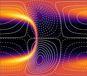
Figure 2. Snapshots of full states, in terms of  $\mathrm {tr} \, \boldsymbol{\mathsf{C}}$ (contours), at the saddle-node bifurcation points from figure 1. Lines correspond to level sets of the perturbation stream function. The noticeable thinning of the arrowhead structure with increasing $Re$ (from bottom right to top left) is partially due to the corresponding increase in $k_{opt}$ (and decrease in domain length; see § 4.2 and compare with figure 5). The domain size is $2 {\rm \pi}/ k_{opt}$ in the $X$ direction, with $k_{opt} \in \{4.7,2.7,1.8,1.6\}$ in panel order.

Figure 3. (a) Contours of  $\hat {u}_X/u_{b,X}$ at the saddle-node point of the $Re = 200$ branch (blue triangle in figures 1 and 2). The domain length is $2 {\rm \pi}/ 2.7$ as in figure 2. (b) Same as (a) but with $\hat {u}_y/u_{b,X}$ displayed. (c) Mean velocity profiles $u_X/u_{b,X}$ at the saddle-node points marked on figures 1 and 2, with colour codes matching that of figure 1.

Figure 4. (a) The  $Re = 60$ branch from figure 1, with edge states indicated by the dashed line. (b) Results of the independent edge-tracking algorithm at $Wi=20$. The blue/red lines indicate evolutions which start close to the lower branch state and converge to the laminar/upper branch state, respectively.
Based on these observations, we have the following picture: if the laminar state is disturbed with a perturbation large enough to reach a certain threshold, determined by the minimal amplitude of approach of the stable manifold of a lower branch state, the flow will evolve towards the upper branch, forming a stable TW. The threshold amplitude to trigger growth is bounded above by the amplitude of the lower branch state itself, which remains  $\mathcal {A} < 1.05$ across the domain of existence of TWs. In other words, this domain (shaded bright grey on figure 1) is nonlinearly unstable when subjected to finite but small amplitude disturbances.
4.2. Influence of domain length
This section is dedicated to studying the effect of  $k$, and thus the influence of domain size $[0,2 {\rm \pi}/k]$, on the TWs. Figure 5 shows how a single branch of TWs at $Re = 30$ (purple in figure 1) changes with $k$. It has already been established that the steady arrowhead structure is highly sensitive to domain length in the EIT regime (Dubief et al. Reference Dubief, Page, Kerswell, Terrapon and Steinberg2022). There, through capturing larger-scale motions, an increase in domain length was found to unveil structures of increasing complexity, with the possibility of inducing chaotic dynamics at certain parameter combinations. Similar tendencies can be observed in our case (cf. figure 5): An increase in $k$ (and, thus, decrease in domain length) has a considerable weakening effect on the arrowhead structure, eventually resulting in a complete eradication of TWs and a subsequent relaminarization. Despite this observation, the location of the saddle-node points seems largely unaffected by $k$ (cf. figure 5), making the marked ‘nonlinearly unstable’ region on figure 1 robust to changes in the assumed periodicity and domain size.

Figure 5. (a) Branches of TWs at different wave numbers, and thus domain sizes, at  $k = 1$ (full line), $k$
$k$  $(= k_{opt})= 1.6$ (dashed line) and $k = 2$ (dotted line) with fixed $Re=30$ ( $k=1.6$ is also shown coloured purple in figure 1). (b) Snapshots of $k = 1$ and $k = 2$ upper branch TWs at fixed $Wi= 19.814$ (note the difference in domain size). Contours correspond to $\mathrm {tr} \, \boldsymbol{\mathsf{C}}$ and lines correspond to level sets of the perturbation stream function. All visible differences are contained in the superimposed wave solutions: the laminar state does not depend on $k$.
$k$.
4.3. High-elasticity regime: $Re \rightarrow 0$

The high-elasticity regime is difficult to access using time-stepping as it becomes increasing stiff as  $Re \rightarrow 0$. The algebraic approach taken here suffers no such problems and we can approach and even consider $Re=0$ (see the next section) without difficulty.
The existence of the centre-mode linear instability at  $Re = 0$ is already known in the limit of very dilute polymer solutions ( $\beta \to 1$) for $Wi = O (10^{3})$ in Oldroyd-B fluids (Khalid et al. Reference Khalid, Shankar and Subramanian2021b) and for $Wi = O (10^{2})$ in FENE-P fluids at finite extensibility ( $L_{max}$) (Buza et al. Reference Buza, Page and Kerswell2022). To substantiate its connection to ET, the time evolution of these growing modes has to be tracked to see whether they are able to produce turbulent behaviour, presumably after transitioning through a cascade of intermediate states. Our goal here is to see where the first level of intermediate state, the TWs, exist at low and vanishing $Re$.
$Re$.
Weakly nonlinear theory predicts supercritical behaviour in the high elasticity ( $Wi/Re$) regime, i.e. along the lower boundary of the linearly unstable region. To probe this, a fifth branch was initiated at fixed $Wi = 60$, starting upwards in $Re$ as indicated by the weakly nonlinear analysis (Buza et al. Reference Buza, Page and Kerswell2022) from a marginally stable point in this region (indicated by orange on figure 1). The resulting branch of solutions is shown in figure 6. Given the supercriticality, this branch starts off as a stable node, moving up in $Re$. Almost immediately after leaving the initial bifurcation point (of linear stability), it reaches a saddle-node bifurcation point, turns around and proceeds to advance towards decreasing $Re$, maintaining a relatively low amplitude until reaching a second saddle node and transitioning to the upper branch. This is an example of how local information provided by weakly nonlinear analysis can be misleading. In fact, the neutral curve gives rise to TWs which reach to lower $Wi$ at fixed $Re$ and lower $Re$ at fixed $Wi$ as shown by figure 1. Upon further inspection, it turns out that the lower (secondary) fold shown in figure 6 at $Re \approx 30$ is purely a feature of the polymer diffusion term $1/(Re\, Sc) {\rm \Delta} \boldsymbol{\mathsf{C}}$ growing artificially large (as $Re$ is decreased), the effect of which is already known to destroy small-scale dynamics (Dubief et al. Reference Dubief, Page, Kerswell, Terrapon and Steinberg2022). It turns out that the point at which the saddle-node bifurcation occurs can be delayed arbitrarily by adjusting $Sc$ in accordance with the variations in $Re$ to keep the polymer diffusion finite. Numerical experimentation suggested a revised polymer diffusion term of the form
 \begin{equation} \frac{\lambda}{Wi} {\rm \Delta} \boldsymbol{\mathsf{C}}, \end{equation}
for some fixed number  $\lambda$. The choice of an inverse scaling with $Wi$ is motivated by observations at $Re = 0$ shown in Appendix C. If $\lambda = 0.005$ is enforced for the branch in question, which amounts to fixing the coefficient $1/(Re\, Sc)$ at the point marked by ‘ $+$’ in figure 6, the branch of solutions can be followed down to $Re = 0$ along the lower branch (cf. the dashed line in figure 6).

Figure 6. Solution branch at fixed  $Wi = 60$, indicated by orange on figure 1 ( $k = 1$). The solid black line shows the weakly nonlinear prediction of supercriticality. In orange are the results from branch continuation with the $1/(Re\, Sc)$ formulation (full line) and with the $\lambda$ formulation (dashed line) ( $\lambda = 0.005$ and $Sc = 250$) which shows that the branch of TWs quickly turns around and heads to lower $Re$, i.e. the TWs are substantially subcritical.
5. Results: TWs in the creeping flow limit $Re = 0$

Once  $Re = 0$ is reached, we redirect the continuation tool towards decreasing $Wi$. The resulting branch takes the familiar shape (from the $Re>0$ cases) shown in figure 7, attaining its saddle-node bifurcation point at $Wi \approx 7.5$, which serves as a lower bound for the region where TWs exist (note the waves found by Morozov (Reference Morozov2022), at $Re=0$ are all above $Wi=20$, albeit with a different model). Figure 7 gives a detailed description of this branch, containing snapshots of full states that illustrate how these waves evolve as $Wi$ is varied. Arrowhead-shaped structures are still clearly visible at low $Wi$ (cf. panels on the left-hand side of figure 7), establishing their prevalence even in the high-elasticity regime. We also report the phase speed, $c$, of the inertialess TWs as a function of $Wi$ in figure 7. Similar to the elasto-inertial case reported in Page et al. (Reference Page, Dubief and Kerswell2020), the phase speed is always faster than the bulk velocity. On the lower branch, $c$ tends to a constant value which matches that of the linear eigenfunction. The phase speed of the upper branch solution is notably slower, and is presumably set by the self-sustaining mechanism proposed by Morozov (Reference Morozov2022).

Figure 7. (Middle right) Branch of TWs at  $Re = 0$, $\beta = 0.9$, $L_{max} = 500$, $\lambda = 0.005$, $k=1$ in terms of the amplitude $\mathcal {A}$ and wavespeed $c$ (here the unstable lower branch is distinguished via dashes). All other panels correspond to states at the locations marked via different symbols. In these plots, contours correspond to $\mathrm {tr} \, \boldsymbol{\mathsf{C}}$ and lines correspond to level sets of the perturbation stream function. Domain length is $2 {\rm \pi}$ in all state plots.
For the particular case considered in figure 7 (specifically  $k=1$, $L_{max}=500$, $\lambda =0.005$) the stability of steady states was examined along the upper branch using DNS. At four points, $Wi = 10,20,30$ and $50$, solutions of the branch continuation tool were transferred into the Dedalus-based DNS code, and were subsequently subjected to disturbances of finite amplitude. The perturbations were constructed from snapshots extracted from separate simulations of EIT at high- $Re$, which were pre-multiplied by $10^{-6}$ and added to the TWs. All perturbed states returned to their respective stable upper-branch solutions after a period of transient growth, suggesting that two-dimensional ET cannot be initiated from these TWs in a direct manner.
5.1. $\beta \in [0.5,1)$: relation to recent experiments

The first experiments claiming to see nonlinear instability in viscoelastic channel flow were performed by Arratia and colleagues (Pan et al. Reference Pan, Morozov, Wagner and Arratia2013; Qin & Arratia Reference Qin and Arratia2017; Qin et al. Reference Qin, Salipante, Hudson and Arratia2019). Finite-amplitude perturbations were induced by an array of obstacles placed upstream, with the number of obstacles serving as a measure of amplitude. Based on measurements taken further downstream, far away from the initial disturbances, they conclude the existence of a subcritical nonlinear instability that persists down to  $Wi \approx 5.4$. With the caveats that their channel had a square cross-section and FENE-P is an approximation, their results are encouragingly comparable to the two-dimensional channel prediction made here of $Wi_{sn}=7.5$. In Figure S1 of the supplementary material to Pan et al. (Reference Pan, Morozov, Wagner and Arratia2013), the authors indicated the boundary to the observed instability in a $Wi$ versus perturbation amplitude plane, essentially matching our predictions for the threshold of nonlinear instability given by the $Re = 0$ lower branch (shown in the middle-right panel of figure 7) (that the unstable region in our case is bounded by the branch is an immediate consequence of the discussion in § 4.1: once the threshold amplitude of a lower branch edge state is reached, solutions continue to grow). However, in later proceedings, the authors claim that the unstable flow remains time dependent with features reminiscent of ET (Qin & Arratia Reference Qin and Arratia2017; Qin et al. Reference Qin, Salipante, Hudson and Arratia2019), as opposed to the upper branch TW scenario described here.
More recently, (Schnapp & Steinberg Reference Schnapp and Steinberg2022) have experimentally examined the stability of viscoelastic channel flow to small disturbances using a channel of width-to-height ratio of 7. The viscosity ratio was  $\beta = 0.74$ and so significantly smaller than the above presented $\beta = 0.9$. They describe seeing a complex transition which they call ‘an elastic non-normal mode instability’ characterised by the direct transition to many modes at once. This is different from a modal instability of a TW solution discussed here but may also be the effect of a comparatively large initial disturbance so the transition is immediately strongly nonlinear. Other recent experiments by Choueiri et al. (Reference Choueiri, Lopez, Varshey, Sankar and Hof2021) in a pipe have also considered smaller $\beta =0.57$ albeit at larger $Re$. Motivated by this, we also performed a few TW branch continuations (at $Wi = 10, 20, 30$ and $50$) with decreasing $\beta$ in an attempt to map out the nonlinearly unstable domain in the $Wi\unicode{x2013}\beta$ plane (all with zero inertia). Results from these computations are shown in figure 8, with the left panel indicating the unstable region and the right panel containing the solution branches found with varying $\beta$. It transpires that at lower $\beta$, the solutions are a little more sensitive to the artificial diffusion (see Appendix C for further details), necessitating multiple simulations at different $\lambda$ values, all of which are also shown in figure 8.

Figure 8. (a) Nonlinearly unstable regions in the  $Wi$–
$Wi$– $\beta$ plane at $Re = 0$ for $\lambda = 0.005$ (full line), $\lambda = 0.003$ (dashed line) and $\lambda = 0.002$ (dotted line). Horizontal and vertical lines correspond to solution branches computed via the continuation routine. (b) Branches with respect to $\beta$, obeying the same colour code as on the left panel (at $\lambda = 0.005$).
Figure 9 tracks changes in the lower branch TW amplitude, which is an upper bound on the threshold for growth, as  $Wi$ is increased. For the parameter combination in question ( $\beta = 0.74$, $Re = 0$), both our standard amplitude measure $\mathcal {A}$ and a separate measure for the magnitude of velocity perturbations, $\Vert \hat {\boldsymbol u} \Vert _{L^{2} (\varOmega )}$, are shown. For $Wi > 30$, $\mathcal {A}$ remains below $1.005$, implying that perturbations amounting to just $0.5\,\%$ of the laminar conformation field $\mathrm {tr} \, \boldsymbol{\mathsf{C}}_b$ are sufficient to trigger growth, making this scenario practically indistinguishable from a linearly unstable one. Here $\mathcal {A}$ reaches its minimum roughly around $Wi = 100$, then, despite setting off in an increasing trend, remains negligibly small up to $Wi=500$.

Figure 9. (a) The  $\beta = 0.74$ lower branch from figure 8, at $\lambda = 0.001$, with respect to the standard amplitude measure $\mathcal {A}$ (in black) and the perturbation velocity magnitude $\Vert \hat {\boldsymbol u} \Vert _{L^{2} (\varOmega )}$ (in blue). (b) State snapshot at $Wi = 20$ from the branch above. Contours show $\hat {u}_X/u_{b,X}$. (c) State snapshot at $Wi = 407$ from the branch above. Contours show $\hat {u}_X/u_{b,X}$.
In addition to the solution branch, figure 9 also displays two state plots at  $Wi = 20$ and $Wi = 407$, now in terms of $\hat {u}_X/u_{b,X}$ to aid comparison with experimental results. The former, at $Wi = 20$, still resembles the structural composition of the linearly unstable centre eigenmode at higher $Re$: chevron-shaped streaks remain visible, but are now disconnected at the centreline. However, by $Wi = 407$ (and similarly for all $Wi>100$ lower branch states), these structures straighten out and form streamwise counter-propagating streaks placed symmetrically around the centreline.
In their pipe set-up, Choueiri et al. (Reference Choueiri, Lopez, Varshey, Sankar and Hof2021) detected fluctuations at  $Re \approx 5$ for $\beta = 0.57$, $Wi = 104$ while the flow remained laminar at $Re \approx 3$. Computationally, the $Re=0$ branch may be continued to $\beta = 0.57$ (for $\lambda$ sufficiently small) in our channel flow setting (cf. figure 8 again), albeit with a slightly larger threshold amplitude than that of figure 9. This may explain the need for a finite $Re$ for ‘unperturbed’ instabilities (Choueiri et al. Reference Choueiri, Lopez, Varshey, Sankar and Hof2021). Interestingly, the flow states shown by Choueiri et al. (Reference Choueiri, Lopez, Varshey, Sankar and Hof2021) have the connected, chevron-shaped streaks reminiscent of the centre-mode eigenfunction. In our setting, ‘connectedness’ of the chevrons is lost shortly after leaving the initial bifurcation (the general shape is still retained for moderate $Wi$, see the middle panel of figure 9), but the scenario could be quite different in pipes.
5.2. $L_{max} \in \{70,100,500\}$

For completeness, the effect of varying the last outstanding parameter,  $L_{max}$, on the region of nonlinear instability is depicted in figure 10. In contrast to the observations of Buza et al. (Reference Buza, Page and Kerswell2022), which indicated that lowering $L_{max}$ has a destabilizing role in the elastically dominated regime (cf. their figure 13), here we see that the nonlinearly unstable region shrinks with decreasing $L_{max}$. This suppressing effect is in line with past observations of the effect of finite extensibility; see, e.g., the linear analyses in Ray & Zaki (Reference Ray and Zaki2014), Page & Zaki (Reference Page and Zaki2015) or even figure 16 of Buza et al. (Reference Buza, Page and Kerswell2022). It should be noted that, in our experience, solution branches became difficult to extract at lower $L_{max}$, with convergence issues appearing along upper branches. In fact, we can only reliably obtain upper branches for $L_{max}>150$, but lower branches remain accessible due to their lower resolution requirements (see Appendix B).

Figure 10. The effect of varying  $L_{max}$ on the nonlinearly unstable region at fixed $\lambda = 0.003$. Horizontal and vertical lines correspond to solution branches computed via the continuation routine with $L_{max} = 70$ (black solid lines), $L_{max} = 100$ (red dashed lines) and $L_{max} = 500$ (blue dotted lines).
6. Discussion
In this paper, we have used branch continuation to track two-dimensional, finite-amplitude TWs in a viscoelastic channel flow, using the FENE-P model. The TWs are borne out of the centre mode instability (Khalid et al. Reference Khalid, Chaudhary, Garg, Shankar and Subramanian2021a) which is known to be subcritical over large areas of the  $Re-Wi$ parameter space (Buza et al. Reference Buza, Page and Kerswell2022). Here, we have shown that the TW solution branches extend to significantly lower $Re$ and $Wi$ than the curve of marginal stability. For instance, we showed that the saddle node at $Re=1000$ drops as low as $Wi\approx 25$, while the associated linear instability at this $Re$ does not occur until $Wi\approx 80$. Most significantly, we demonstrated the persistence of the nonlinear TWs at $Re=0$ for a large range of $Wi$, with the saddle node sitting at $Wi \approx 7.5\unicode{x2013}10$ in dilute ( $\beta =0.9$) solutions for a range of $L_{max}$. Across a broad range of the parameter space, including at $Re=0$, the upper branch TWs resemble the arrowhead structures observed in DNS at higher $Re$ (Page et al. Reference Page, Dubief and Kerswell2020; Dubief et al. Reference Dubief, Page, Kerswell, Terrapon and Steinberg2022).
A key feature of the solution branch at  $Re=0$ is the low amplitude of the lower branch TW across a very large range of $Wi$. This suggests that only a very weak disturbance would be required to cause the flow to transition to a potentially complicated time-dependent state, a scenario which would potentially be indistinguishable from a linear instability in an experiment. The small amplitude of the lower branch also poses the question whether the amplitude expansion pursued in Morozov & Saarloos (Reference Morozov and van Saarloos2005) and Morozov & van Saarloos (Reference Morozov and van Saarloos2019) was attempting to resolve it; see, e.g., figure 8(c) of Morozov & van Saarloos (Reference Morozov and van Saarloos2019).
While our results demonstrate the existence of finite-amplitude arrowhead TWs over a very large range of the parameter space, a direct connection to either EIT or ET has yet to be established even within the same FENE-P model. In inertia-dominated EIT at Reynolds numbers  $Re=O(1000)$, instantaneous arrowhead-shaped flow structures resembling the stable upper branch states have been observed numerically (Dubief et al. Reference Dubief, Page, Kerswell, Terrapon and Steinberg2022). While the region of nonlinear instability found here overlaps with these observations, further work is required to assess if there is a direct connection between the exact coherent states and EIT (e.g. through a sequence of successive bifurcations). The picture is complicated by observations from both numerics and experiments at higher $Re$, where near-wall activity has been observed to be dominant in both channels and pipes (Shekar et al. Reference Shekar, McMullen, Wang, McKeon and Graham2019, Reference Shekar, MucMullen, McKeon and Graham2020; Choueiri et al. Reference Choueiri, Lopez, Varshey, Sankar and Hof2021). At present, no exact coherent states connected to other linear instabilities (e.g. Tollmien–Schlichting waves in channels, see Shekar et al. Reference Shekar, McMullen, Wang, McKeon and Graham2019) have been discovered, and the possible role of such states in EIT remains an interesting open problem. At low $Re$, our numerical experiments indicate that the upper branch TWs are linearly stable, and we have been unable to trigger ET. Our computations have been restricted to two-dimensional flows, and so this does not rule out the existence of ET in three dimensions, or a direct route from the upper branch TWs to such a state. We hope to report results on this soon.
Acknowledgements
GB gratefully acknowledges the support of the Harding Foundation through a PhD scholarship (https://www.hardingscholars.fund.cam.ac.uk).
Funding
MB, RK and JP thank EPSRC for support under grant EP/V027247/1.
Declaration of interests
The authors report no conflict of interest.
Data availability statement
The numerical codes used in this work are available at https://doi.org/10.17863/CAM.89385.
Appendix A. Pseudo-arclength continuation
The branch continuation routine is launched from a point on the neutral curve (curve of marginal linear stability) with the aid of the weakly nonlinear theory, which provides the very first initial condition near the solution branch of interest. Beyond this point, as parameters are varied in larger increments, supplying sufficiently accurate initial conditions for (3.14) amounts to predicting the shape of the bifurcation branch, precisely the objective of pseudo-arclength continuation (see, e.g., Dijkstra et al. Reference Dijkstra2014).
If  $\kappa \in \{Wi, Re, \beta \}$ is the parameter allowed to vary in the continuation (all others are fixed), $\mathcal {F}$ restricts to a map $\mathcal {F}: \mathbb {R}^{Q+1} \to \mathbb {R}^{Q}$ and (3.14) translates to
 \begin{equation} \mathcal{F}(\boldsymbol a,c,F_X,\kappa) = \boldsymbol{0}.\end{equation}
 Arclength-based techniques interpret the branch of solutions as a curve  $\boldsymbol {\gamma } : \mathbb {R} \to \mathbb {R}^{Q+1}$ embedded in configuration space, which is spanned by $(\boldsymbol a,c,F_X,\kappa )$ in this particular case. Assume now that a steady state has been computed at point $n$ on the branch $\boldsymbol {\gamma }$, which we write as $\boldsymbol {\gamma }(t_n) = (\boldsymbol a_n,c_n,F_{X,n},\kappa _n)^{\rm T}$. A prediction for the solution at the next step, $\boldsymbol {\gamma }(t_{n+1})$, is given by moving a distance of $s$ tangentially along $\boldsymbol {\gamma }$, where $s$ denotes the a priori specified step size. Making use of the fact that a solution branch must satisfy $\mathcal {F} \circ \boldsymbol {\gamma } \equiv \boldsymbol {0}$, the tangent at point $n$ is computed according to
 \begin{equation} \begin{pmatrix} D \mathcal{F} (\boldsymbol{\gamma} (t_n)) \\ \dot{\boldsymbol{\gamma}}(t_{n-1})^{\rm T} \end{pmatrix} \dot{\boldsymbol{\gamma}} (t_n) = \begin{pmatrix} \boldsymbol{0} \\ 1 \end{pmatrix}. \end{equation}
If no tangent is available at the previous step, the last row is replaced by  $(0,\ldots,1)$. The initial prediction for the solution at step $n+1$ is given by
 \begin{equation}
\tilde{\boldsymbol{\gamma}}^{0} (t_{n+1}) :=
\begin{pmatrix} \boldsymbol a_{n+1}^{0} \\ c_{n+1}^{0} \\
F_{X,n+1}^{0} \\ \kappa_{n+1}^{0} \end{pmatrix} =
\boldsymbol{\gamma}(t_n) + s \dot{\boldsymbol{\gamma}}
(t_n),\end{equation}
\begin{equation}
\tilde{\boldsymbol{\gamma}}^{0} (t_{n+1}) :=
\begin{pmatrix} \boldsymbol a_{n+1}^{0} \\ c_{n+1}^{0} \\
F_{X,n+1}^{0} \\ \kappa_{n+1}^{0} \end{pmatrix} =
\boldsymbol{\gamma}(t_n) + s \dot{\boldsymbol{\gamma}}
(t_n),\end{equation}
where the upper indices correspond to the number of completed Newton–Raphson iterates (see the following), and the twiddle serves to distinguish the converged branch  $\boldsymbol {\gamma }$ from its approximate counterpart $\tilde {\boldsymbol {\gamma }}$. The next step is to employ the Newton–Raphson method using (A3) as initial condition to obtain an exact solution of (A1). Knowledge of the tangent may be used to aid this procedure, by means of constraining subsequent iterates to remain on the hyperplane orthogonal to $\dot {\boldsymbol {\gamma }} (t_n)$. Incorporating this condition into a standard Newton–Raphson scheme, we obtain the system
 \begin{equation} \begin{pmatrix} D
\mathcal{F}(\tilde{\boldsymbol{\gamma}}^{i} (t_{n+1}) ) \\
\dot{\boldsymbol{\gamma}}(t_n)^{\rm T} \end{pmatrix} {\rm \Delta}
\tilde{\boldsymbol{\gamma}}^{i+1}(t_{n+1}) =
\begin{pmatrix}
-\mathcal{F}(\tilde{\boldsymbol{\gamma}}^{i} (t_{n+1})) \\
s- \langle \dot{\boldsymbol{\gamma}}(t_n) ,
\tilde{\boldsymbol{\gamma}}^{i} (t_{n+1}) -
\boldsymbol{\gamma}(t_n) \rangle \end{pmatrix},
\end{equation}
\begin{equation} \begin{pmatrix} D
\mathcal{F}(\tilde{\boldsymbol{\gamma}}^{i} (t_{n+1}) ) \\
\dot{\boldsymbol{\gamma}}(t_n)^{\rm T} \end{pmatrix} {\rm \Delta}
\tilde{\boldsymbol{\gamma}}^{i+1}(t_{n+1}) =
\begin{pmatrix}
-\mathcal{F}(\tilde{\boldsymbol{\gamma}}^{i} (t_{n+1})) \\
s- \langle \dot{\boldsymbol{\gamma}}(t_n) ,
\tilde{\boldsymbol{\gamma}}^{i} (t_{n+1}) -
\boldsymbol{\gamma}(t_n) \rangle \end{pmatrix},
\end{equation}
supplemented with the update rule
 \begin{equation} \tilde{\boldsymbol{\gamma}}^{i+1} (t_{n+1}) = \tilde{\boldsymbol{\gamma}}^{i} (t_{n+1})+{\rm \Delta} \tilde{\boldsymbol{\gamma}}^{i+1}(t_{n+1}). \end{equation}
Once the solutions have converged to a sufficient degree, i.e.
 \begin{equation} \frac{|{\rm \Delta} \tilde{\boldsymbol{\gamma}}^{i+1}(t_{n+1})|}{|\tilde{\boldsymbol{\gamma}}^{i} (t_{n+1})|}< {tol}, \end{equation}
is reached, we set  $\boldsymbol {\gamma }(t_{n+1}) = \tilde {\boldsymbol {\gamma }}^{i+1}(t_{n+1})$, and continue further along the branch. The tolerance ‘ $\mathrm {tol}$’ was set to $10^{-8}$ throughout all examples shown. The continuation routine consists of repeated applications of the above procedure over $n$, resulting in a discrete representation of the full solution branch as $\{\boldsymbol {\gamma } (t_n)\}_{n \geq 0}$.
Appendix B. Resolution
Figure 11 shows how different truncations in the branch continuation and DNS compare when resolving the upper and lower TWs shown in figure 4 at  $Wi=20$ (more precisely $(Wi,Re,\beta,Sc, L_{max})=(20,60,0.9,250,500)\,$) with the base flow subtracted. The various truncations of branch continuation show very good agreement with the spectra from the DNS. It is worth remarking that to obtain converged spectra in the DNS it was necessary to reduce the timestep to ${\rm \Delta} t=1\times 10^{-3}$. Further discrepancies for the higher-order modes may be caused by the finite accuracy of the edge tracking algorithm in locating the lower branch.

Figure 11. Grid independence checks at  $Re = 60$, $Wi = 20$, $L_{max} = 500$, $\beta = 0.9$ and $Sc = 250$ for both the upper and lower branch solutions. The upper branch is identified by larger coefficient contributions. Orange, yellow, red and green lines with symbols correspond to solutions obtained through branch continuation, the blue solid lines correspond to the DNS detailed in § 3.2 using $N_X=128$ complex Fourier modes and $N_y=128$ Chebyshev coefficients. (a) $N_y$ independence: Overall contribution of each Chebyshev mode for $N_y\in \{30,40,50,60\}$ for the lower branch and $N_y\in \{35,50,60,70\}$ for the upper branch, with $N_X = 60$ fixed in the branch continuation. (b) $N_X$ independence: Overall contribution of each Fourier mode for $N_X\in \{20,40,60,80\}$ for the lower branch and $N_X\in \{30,40,60,80\}$ for the upper branch, with $N_y = 60$ fixed in the branch continuation.
Appendix C. Remarks on the polymer diffusion term
Memory limitations associated with increasing  $N_X$ and $N_y$ provide an upper bound on how large a value of $Sc$ can be considered whereas taking $Sc$ too small is known to eradicate small scale dynamics. Thus, $Sc$ was selected between the two of these bounds: just above the smallest number where solution branches become independent of $Sc$, but resolution requirements are still moderate enough for the physical memory to handle.
In the creeping flow limit ( $Re \rightarrow 0$), a distinguished limit with $Sc \rightarrow \infty$ such that $Sc=1/(\varepsilon Re)$ with $\varepsilon$ a constant clearly needs to be taken to retain finite polymer diffusion as follows
 \begin{equation} \partial_t \boldsymbol{\mathsf{C}} + ( \boldsymbol u \boldsymbol{\cdot} \boldsymbol{\nabla}) \boldsymbol{\mathsf{C}} + \boldsymbol{\mathsf{T}}(\boldsymbol{\mathsf{C}}) = \boldsymbol{\mathsf{C}} \boldsymbol{\cdot} \boldsymbol{\nabla} \boldsymbol u + ( \boldsymbol{\nabla} \boldsymbol u )^{\rm T} \boldsymbol{\cdot} \boldsymbol{\mathsf{C}} + \varepsilon {\rm \Delta} \boldsymbol{\mathsf{C}}. \end{equation}
The new polymer diffusion coefficient,  $\varepsilon$, is selected analogously to $Sc$, whereby independence of solution branches is sought while keeping the grid size manageable. Numerical observations indicate that there cannot be a universal $\varepsilon$ that is optimal in this sense across all parameter regimes within the $Re=0$ limit. However, the slight rescaling $\lambda = \varepsilon Wi$ (cf. § 4.3) seems to help.Figure 12 displays three pairs of solution branches computed at different values of fixed $\lambda$ (in green) and fixed $\varepsilon$ (in blue). While the $\lambda$-based branches can be extended up to arbitrarily large $Wi$ (the $\lambda = 0.005$ one was continued up to $Wi > 1000$, not shown), the $\varepsilon$-based ones form isolas at low Weissenberg numbers $Wi < 30$, resulting in a loss of robustness with respect to $\varepsilon$. Using $\lambda$, robustness is recovered after a certain threshold is hit ( $\lambda \approx 0.007$ for this branch), which served as the primary motivation behind choosing $\lambda$ as the parameter to be fixed throughout the main text.

Figure 12. Solution branches at fixed  $\lambda = 0.005$ (full line), $\lambda = 0.007$ (dashed line), $\lambda = 0.01$ (dotted line). Inset: Branches with $\varepsilon$ fixed, at $\varepsilon = 5 \times 10^{-4}$ (full line), $\varepsilon = 7 \times 10^{-4}$ (dashed line) and $\varepsilon = 10^{-3}$ (dotted line), so that they agree with their $\lambda$-based counterparts at $Wi = 10$.


 Open access