


1 Introduction
Turbulent jets, plumes and thermals are prevalent in nature and technology. Jets and plumes are continuous streams of, respectively, non-buoyant or buoyant fluid forced out of a small opening. The instantaneous release of a parcel of buoyant liquid from such a source is referred to as a thermal. The investigation of the flow dynamics associated with these flows has developed a long-standing history (Morton, Taylor & Turner Reference Morton, Taylor and Turner1956; Scorer Reference Scorer1957; Turner Reference Turner1962; List Reference List1982; Reynolds et al. Reference Reynolds, Parekh, Juvet and Lee2003; Woods Reference Woods2010).
The present study investigates turbulent jets, i.e. water that is being ejected continuously into an ambient environment of water of equal density. Moreover, the jets considered are generated within a system rotating at velocity
 $\unicode[STIX]{x1D6FA}$
, that is, they are ejected into ambient water that is in solid-body rotation. The direction of ejection is aligned parallel with the axis of rotation.
$\unicode[STIX]{x1D6FA}$
, that is, they are ejected into ambient water that is in solid-body rotation. The direction of ejection is aligned parallel with the axis of rotation.
In the remainder it will be seen that the type of jets discussed here develop a cyclonically swirling flow motion, relative to the axis of the background rotation. This swirl arises due to effects of Coriolis forces on the radial flow that is induced when the primary jet flow establishes radial motion due to entrainment of ambient water while propagating away from the exit nozzle. Therefore these jets are, in some respect, qualitatively similar to swirling jets in a non-rotating environment – the latter having been the subject of numerous studies in the past (e.g. Billant, Chomaz & Huerre Reference Billant, Chomaz and Huerre1998; Liang & Maxworthy Reference Liang and Maxworthy2005). Nevertheless, the boundary conditions in both flow scenarios are in fact fundamentally different. For studies on traditional swirling jets, a swirl is deliberately enforced and this swirling liquid is then injected into a stationary liquid. However, for the jets considered here, non-swirling liquid is injected into a stationary liquid, but within a rotating frame of reference. Thereafter swirl within the jet, and relative to the rotating flow, develops gradually as a consequence of Coriolis forces acting on the radial flow component. Thus, for traditional swirling jets the swirl pre-exists at the moment when the liquid is injected into the stationary, ambient, non-rotating liquid. Thereafter, the swirling jet begins to induce rotation onto liquid in its immediate exterior vicinity by diffusive momentum transfer such that the swirl concurrently reduces due to viscous dissipation for increasing distance from the source of injection. Nevertheless, in the case of the current study, swirling motion, relative to the system rotation as a whole, develops gradually due to Coriolis forces. Thus, the type of jets considered here and traditional swirling jets differ fundamentally insofar as the aspect of causes and effects of their flow dynamics are concerned.
One focus of the current study is a time-periodic formation–breakdown cycle of jets developing subject to background rotation, which does not appear to have been observed experimentally in the past. Previously the process only seems to have been referred to in a recent, short publication by Lawrie et al. (Reference Lawrie, Duran, Scott, Godeferd, Flor, Cambon and Daniaila2011) summarizing computational simulations of the type of flow considered here. Note again that we address the case where there exists no density difference between the liquid of the ejected jet and the ambient environment. Oscillatory behaviour associated with thermals, where buoyancy effects are present, have previously already been predicted theoretically by, for instance, Wilkins et al. (Reference Wilkins, Sasaki, Friday, McCarthy and McIntyre1969). It appears, however, that they did not observe this behaviour in their experiments, since they state that the predicted period of oscillation is long compared with the life of their simulated thermals.
Jets in rotating flow were first considered theoretically by Barcilon (Reference Barcilon1967) in the context of analysing the dynamics of dust devils. Barcilon (Reference Barcilon1967) extended the similarity solutions obtained by Morton et al. (Reference Morton, Taylor and Turner1956), for maintained and instantaneous sources in a non-rotating fluid, to the case of a rotating fluid. The first experimental laboratory study investigating the effects of background rotation on such types of flows appears to be that performed by Wilkins et al. (Reference Wilkins, Sasaki, Friday, McCarthy and McIntyre1969) to simulate thermals in a rotating fluid. They considered the instantaneous release of liquid with injection periods of approximately 0.2 s.
The study of Wilkins et al. (Reference Wilkins, Sasaki, Friday, McCarthy and McIntyre1969) motivated Niino (Reference Niino1978, Reference Niino1980) to extend their work theoretically and experimentally. He considered the cases of instantaneous and maintained liquid releases and, in particular, Niino (Reference Niino1978, Reference Niino1980) addressed the case that is the subject of the current study, where there exists no density difference between the ejected and the ambient liquid.
The theoretical considerations of Niino (Reference Niino1980) show that jets in a rotating fluid are subject to the buildup of an axial pressure gradient in the forcing region which acts to oppose the forcing. Niino (Reference Niino1980) describes that, for the case of continuous forcing, the pressure gradient becomes nearly steady after a certain time interval, but he does not refer to any time-periodic features that could be related to the formation–breakdown cycle that is the subject of the current investigation. Nevertheless, for forcing of finite duration, but longer than a certain critical limit, the computations of Niino (Reference Niino1980) revealed damped, continuous oscillations near the forcing region, with a period of approximately
 $\unicode[STIX]{x03C0}/\unicode[STIX]{x1D6FA}$
, after the forcing has been terminated. Niino (Reference Niino1980) discusses that these oscillations are associated with reverse flow in the forcing regions at large times but he does not state whether he had indeed observed these oscillations in the earlier experiments (Niino Reference Niino1978) that motivated his subsequent computations. It is, nevertheless, indicated in Niino (Reference Niino1978) that the onset of the reverse flow was observed, as is expressed in the abstract of the article when he states, regarding jets being ejected downwards, that ‘a remarkable upward motion appears when the injection of the source fluid is stopped’. The remainder of the current article will reveal that our experiments have in fact revealed a periodically developing and decaying reverse flow and that this is closely associated with the periodic formation–breakdown cycle of the jets observed in the computations of Lawrie et al. (Reference Lawrie, Duran, Scott, Godeferd, Flor, Cambon and Daniaila2011).
$\unicode[STIX]{x03C0}/\unicode[STIX]{x1D6FA}$
, after the forcing has been terminated. Niino (Reference Niino1980) discusses that these oscillations are associated with reverse flow in the forcing regions at large times but he does not state whether he had indeed observed these oscillations in the earlier experiments (Niino Reference Niino1978) that motivated his subsequent computations. It is, nevertheless, indicated in Niino (Reference Niino1978) that the onset of the reverse flow was observed, as is expressed in the abstract of the article when he states, regarding jets being ejected downwards, that ‘a remarkable upward motion appears when the injection of the source fluid is stopped’. The remainder of the current article will reveal that our experiments have in fact revealed a periodically developing and decaying reverse flow and that this is closely associated with the periodic formation–breakdown cycle of the jets observed in the computations of Lawrie et al. (Reference Lawrie, Duran, Scott, Godeferd, Flor, Cambon and Daniaila2011).
Several experimental studies exist which have investigated plumes and thermals in rotating flow (Elrick Reference Elrick1979; Etling & Fernando Reference Etling, Fernando, Davies and Neves1993; Fernando & Ching Reference Fernando and Ching1993; Ayotte & Fernando Reference Ayotte and Fernando1994; Bush & Woods Reference Bush and Woods1998; Fernando, Chen & Ayotte Reference Fernando, Chen and Ayotte1998). However, all these studies include buoyancy effects and, moreover, they report results of experiments involving dye visualizations only. To date there do not seem to exist any studies investigating non-buoyant jets in a rotating fluid by means of modern particle image velocimetry (PIV). We are currently conducting such a PIV study. The purpose of this summary of results is to report the observation of a time-periodic formation–breakdown cycle associated with jets in a rotating fluid. It appears that this formation–breakdown cycle observed is a manifestation of the behaviour described in the discussion of the computational results of Lawrie et al. (Reference Lawrie, Duran, Scott, Godeferd, Flor, Cambon and Daniaila2011). The PIV results discussed here represent the first experimental verification of the existence of the phenomenon described by Lawrie et al. (Reference Lawrie, Duran, Scott, Godeferd, Flor, Cambon and Daniaila2011).
Lawrie et al. (Reference Lawrie, Duran, Scott, Godeferd, Flor, Cambon and Daniaila2011) conducted a numerical study investigating an axisymmetric jet in a rotating reference frame by means of their MOBILE software. Lawrie et al. (Reference Lawrie, Duran, Scott, Godeferd, Flor, Cambon and Daniaila2011, p. 2) discuss that they observed that the jets develop a helical instability, whereby the jet initially grows, entrains ambient fluid, and that this leads to helical displacement of the jet from the axis. It is reported that at large displacement amplitudes the jet breaks down, upon which the associated entrainment ceases. It is argued that, with nothing to drive further radial convergence of material contours, the azimuthal velocity decays sufficiently for the jet to reform and thereby enables a periodic formation–breakdown cycle to be established. The results presented here will show that our measurements reveal precisely this behaviour.
2 Experimental set-up
The experiments summarized here were conducted using Warwick’s large rotating-tank facility. This facility constitutes a tank of height 2.5 m, with octagonal cross-section and of width 1 m across, which is mounted on top of a rotating turntable. The overall height of the facility, from the floor to the top of the support structure, is over 5.7 m. A technical drawing of the facility can be accessed at the weblink provided in the caption of figure 1.
The jets studied were released vertically upwards from an exit nozzle embedded flush within the top surface of an acrylic ejector box, as illustrated in figure 1. The ejector box had a diameter of 500 mm and it was placed at the bottom of the rotating tank. The centre of the exit nozzle was aligned to coincide with the rotational axis of the turntable. The diameter of the exit nozzle, from which the jets were ejected, was
 $d=6~\text{mm}$
. Thus, the ratio of tank width to source diameter was approximately
$d=6~\text{mm}$
. Thus, the ratio of tank width to source diameter was approximately
 $167$
. This ensured that effects from the surrounding walls of the tank, induced on the flow during the experiments, can be assumed to be negligible. The diameter of the ejector box was chosen much larger than the diameter of the source to ensure that edge effects due to the box periphery were negligible, that is, the jet release approximated ejection from a flat plane of infinite lateral extension.
$167$
. This ensured that effects from the surrounding walls of the tank, induced on the flow during the experiments, can be assumed to be negligible. The diameter of the ejector box was chosen much larger than the diameter of the source to ensure that edge effects due to the box periphery were negligible, that is, the jet release approximated ejection from a flat plane of infinite lateral extension.
The inside of the ejector box contained a layer of a honeycomb-structured aluminium material (cf. figure 1) through which the supplied water had to flow on its path to the exit nozzle. The gap between the top of the honeycomb layer and the bottom surface of the top of the ejector box was approximately 3 cm. The cross-width of each of the individual hexagonal honeycomb cells of the layer was 9.5 mm. The purpose of the honeycomb material was to break up any large-scale rotary flow structures that might potentially develop due to Coriolis forces in the liquid within the ejector box before the water reaches the nozzle exit. Such rotary flow structures could potentially bias the flow condition through swirl being induced on the liquid prior to it being ejected from the exit nozzle.
A controlled, continuous supply of water, at prescribed volumetric flow rate,
 $q_{0}$
, was provided via rotary joints through the hollow central axis of the turntable facility. In preparation for the experiments, the water inside the tank was allowed to settle for at least 4 h after the turntable had been accelerated to its required rotational speed. This ensured that the liquid was in a state of solid-body rotation when the experiments commenced.
$q_{0}$
, was provided via rotary joints through the hollow central axis of the turntable facility. In preparation for the experiments, the water inside the tank was allowed to settle for at least 4 h after the turntable had been accelerated to its required rotational speed. This ensured that the liquid was in a state of solid-body rotation when the experiments commenced.
The laboratory in which the turntable facility is housed is fully air conditioned. Moreover, there exist a number of additional fans distributed throughout the laboratory facilitating agitation and mixing of the ambient air in the laboratory. This ensures that the possibility of vertical temperature gradients developing over long time periods within the liquid inside the tank is minimized.
Flow-field measurements were performed by means of PIV. The entire PIV system was mounted on the rotating turntable, that is, within the rotating frame of reference. The laser of our PIV system is a continuous green class 4 wave laser with wavelength 532 nm and 1000 mW power output. The PIV frames were acquired using a Point Grey USB 3.0 camera at a rate of 90 frames per second and with a resolution of
 $1024\times 1024$
pixels. The images were processed using LaVision Davis 7.2 software. Interrogation areas with
$1024\times 1024$
pixels. The images were processed using LaVision Davis 7.2 software. Interrogation areas with
 $32\times 32$
pixels with
$32\times 32$
pixels with
 $75\,\%$
overlap were used for processing. This configuration leads to a spatial resolution of 2.8 mm. The tracer particles used for the PIV measurements were silver-coated, neutrally buoyant, hollow glass spheres, with a diameter of
$75\,\%$
overlap were used for processing. This configuration leads to a spatial resolution of 2.8 mm. The tracer particles used for the PIV measurements were silver-coated, neutrally buoyant, hollow glass spheres, with a diameter of
 $10~\unicode[STIX]{x03BC}\text{m}$
, supplied by Dantec.
$10~\unicode[STIX]{x03BC}\text{m}$
, supplied by Dantec.
Prior to each experimental run we used the PIV system to verify that the liquid inside the tank had indeed reached solid-body rotation. These tests showed that the residual motion in the measurement planes was below approximately
 $0.08\,\%$
of the typical maximum horizontal and vertical velocities measured in the subsequent experiments. This small magnitude of residual motion also reassures that there existed no significant flows induced by vertical temperature gradients.
$0.08\,\%$
of the typical maximum horizontal and vertical velocities measured in the subsequent experiments. This small magnitude of residual motion also reassures that there existed no significant flows induced by vertical temperature gradients.

Figure 1. Illustration of ejector box and set-up for PIV measurements in the (a) vertical
 $z{-}r$
plane and (b) horizontal
$z{-}r$
plane and (b) horizontal
 $\unicode[STIX]{x1D703}{-}r$
plane. A technical drawing illustrating the scale of Warwick’s large rotating-tank facility, inside which the ejector box is positioned, is displayed as figure S1 in the supplementary material available at https://doi.org/10.1017/jfm.2019.186.
$\unicode[STIX]{x1D703}{-}r$
plane. A technical drawing illustrating the scale of Warwick’s large rotating-tank facility, inside which the ejector box is positioned, is displayed as figure S1 in the supplementary material available at https://doi.org/10.1017/jfm.2019.186.
Two-dimensional (2D) velocity fields were obtained in vertical and horizontal planes. The data are analysed in terms of cylindrical polar coordinates,
 $r,\unicode[STIX]{x1D719},z$
. The
$r,\unicode[STIX]{x1D719},z$
. The
 $z$
-axis coincides with the rotational axis of the turntable and
$z$
-axis coincides with the rotational axis of the turntable and
 $z=0$
corresponds to the centre of the exit nozzle at the surface of the ejector box. The components of the flow velocity associated with
$z=0$
corresponds to the centre of the exit nozzle at the surface of the ejector box. The components of the flow velocity associated with
 $r,\unicode[STIX]{x1D719},z$
are, respectively,
$r,\unicode[STIX]{x1D719},z$
are, respectively,
 $v_{r},v_{\unicode[STIX]{x1D703}},w$
. For measurements with a vertical orientation of the PIV light-sheet plane (cf. figure 1
a), the plane contained the
$v_{r},v_{\unicode[STIX]{x1D703}},w$
. For measurements with a vertical orientation of the PIV light-sheet plane (cf. figure 1
a), the plane contained the
 $z$
-axis and it covered vertical measurement regions with an approximate extent of 350 mm in both streamwise and spanwise directions. When aligned horizontally (cf. figure 1
b), the light sheet could be positioned at variable height above the exit nozzle. Viewing of the flow within the horizontal plane was facilitated by means of a camera mounted at the top of the table through a mirror, located above the liquid surface, as illustrated in figure 1(b).
$z$
-axis and it covered vertical measurement regions with an approximate extent of 350 mm in both streamwise and spanwise directions. When aligned horizontally (cf. figure 1
b), the light sheet could be positioned at variable height above the exit nozzle. Viewing of the flow within the horizontal plane was facilitated by means of a camera mounted at the top of the table through a mirror, located above the liquid surface, as illustrated in figure 1(b).
The experimental conditions for each run of the experiment are characterized in terms of an ejection Reynolds number and an ejection Rossby number. The ejection Reynolds number is defined as
 $Re_{0}=u_{0}d/\unicode[STIX]{x1D708}$
, where
$Re_{0}=u_{0}d/\unicode[STIX]{x1D708}$
, where
 $u_{0}=4q_{0}/\unicode[STIX]{x03C0}d^{2}$
is the mean liquid ejection velocity from the exit nozzle for the liquid supplied at volumetric flow rate
$u_{0}=4q_{0}/\unicode[STIX]{x03C0}d^{2}$
is the mean liquid ejection velocity from the exit nozzle for the liquid supplied at volumetric flow rate
 $q_{0}$
. Similarly, an ejection Rossby number is defined as
$q_{0}$
. Similarly, an ejection Rossby number is defined as
 $Ro_{0}=u_{0}/\unicode[STIX]{x1D6FA}d$
. In § 4.3.2.5, following the discussion of our PIV flow-field measurements of the internal jet structure, it will become possible to introduce an additional, alternative and dynamically more relevant, local Rossby number adopting the definition used by Kloosterziel & van Heijst (Reference Kloosterziel and van Heijst1991) for vortices in a rotating fluid. Experiments were conducted for values of the rotational speed of the turntable facility in the range
$Ro_{0}=u_{0}/\unicode[STIX]{x1D6FA}d$
. In § 4.3.2.5, following the discussion of our PIV flow-field measurements of the internal jet structure, it will become possible to introduce an additional, alternative and dynamically more relevant, local Rossby number adopting the definition used by Kloosterziel & van Heijst (Reference Kloosterziel and van Heijst1991) for vortices in a rotating fluid. Experiments were conducted for values of the rotational speed of the turntable facility in the range
 $0.2~\text{rad}~\text{s}^{-1}\leqslant \unicode[STIX]{x1D6FA}\leqslant 1.1~\text{rad}~\text{s}^{-1}$
with ejection rates for the liquid of
$0.2~\text{rad}~\text{s}^{-1}\leqslant \unicode[STIX]{x1D6FA}\leqslant 1.1~\text{rad}~\text{s}^{-1}$
with ejection rates for the liquid of
 $0.83~\text{cm}^{3}~\text{s}^{-1}\leqslant q_{o}\leqslant 7.5~\text{cm}^{3}~\text{s}^{-3}$
, yielding
$0.83~\text{cm}^{3}~\text{s}^{-1}\leqslant q_{o}\leqslant 7.5~\text{cm}^{3}~\text{s}^{-3}$
, yielding
 $1800\leqslant Re_{0}\leqslant 16\,000$
and
$1800\leqslant Re_{0}\leqslant 16\,000$
and
 $46\leqslant Ro_{0}\leqslant 2100$
.
$46\leqslant Ro_{0}\leqslant 2100$
.
3 Jet development in absence of background rotation
In order to evaluate the reliability and accuracy of the experimental jet apparatus and the PIV measurement system, initial experiments on jets ejected into non-rotating environments were conducted for the purpose of comparison of the results obtained with experimental data by other authors. As part of this comparison summarized below, explicit references will be made to figures from the very recent study by Ezzamel, Salizzoni & Hunt (Reference Ezzamel, Salizzoni and Hunt2015). However, results corresponding to those to be discussed are also contained in other earlier studies by, for instance, Hussein, Capp & George (Reference Hussein, Capp and George1994), Shabbir & George (Reference Shabbir and George1994) or Wang & Law (Reference Wang and Law2002).
Ezzamel et al. (Reference Ezzamel, Salizzoni and Hunt2015) presented experimental measurements conducted on freely propagating, turbulent, steady buoyant air plumes. Thus, in contrast to the present study, the density within their thermal air plumes was different from the density of the ambient air. However, they conducted experiments for conditions ranging from momentum-flux-dominated, jet-like releases to pure plume releases characterized by a balance between momentum, volume and buoyancy fluxes at the source. They focus on the discussion of three different sets of conditions referred to as cases J, F and P in their paper. Of these three cases, the conditions of case J are for jet-like flow conditions for which buoyancy effects are small. Consequently, it is required that the nature and the quality of the experimental data obtained here must mirror those for case J of Ezzamel et al. (Reference Ezzamel, Salizzoni and Hunt2015).
Note that in this section on jets developing in the absence of background rotation, we adopt the nomenclature of Ezzamel et al. (Reference Ezzamel, Salizzoni and Hunt2015) due to the absence of a circumferential flow component in the non-rotating case. The flow in the direction of the vertical
 $z$
-axis remains to be referred to as
$z$
-axis remains to be referred to as
 $w$
. However, the radial component of the flow velocity is referred to by
$w$
. However, the radial component of the flow velocity is referred to by
 $u$
in this section, rather than
$u$
in this section, rather than
 $v_{r}$
as is the case in later sections on results obtained when background rotation is present. Throughout we adopt the display format of Ezzamel et al. (Reference Ezzamel, Salizzoni and Hunt2015) when showing data as a function of the polar coordinate
$v_{r}$
as is the case in later sections on results obtained when background rotation is present. Throughout we adopt the display format of Ezzamel et al. (Reference Ezzamel, Salizzoni and Hunt2015) when showing data as a function of the polar coordinate
 $r$
.
$r$
.
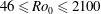
Figure 2. (a) Time-averaged velocity profiles at eight different heights
 $z/d$
as a function of
$z/d$
as a function of
 $r/d$
; (b) collapsed datasets after fitting Gaussian profiles and non-dimensionalizing accordingly for
$r/d$
; (b) collapsed datasets after fitting Gaussian profiles and non-dimensionalizing accordingly for
 $5\leqslant z/d\leqslant 25$
.
$5\leqslant z/d\leqslant 25$
.
3.1 Mean profiles for vertical velocity
 $w(z)$

Figure 2 displays some representative data from the current study for jets in a non-rotating environment released at
 $Re_{0}=3000$
. Figure 2(a) shows seven datasets for the vertical flow-velocity component
$Re_{0}=3000$
. Figure 2(a) shows seven datasets for the vertical flow-velocity component
 $w(r,z)$
, at different non-dimensional heights
$w(r,z)$
, at different non-dimensional heights
 $z/d$
above the source, as a function of the non-dimensional radial position
$z/d$
above the source, as a function of the non-dimensional radial position
 $r/d$
.
$r/d$
.
The vector fields from the PIV measurements were obtained at a rate of 90 frames per second and they were time-averaged over successive periods of
 $\unicode[STIX]{x0394}t=0.25~\text{s}$
. For each profile the velocity data are non-dimensionalized as
$\unicode[STIX]{x0394}t=0.25~\text{s}$
. For each profile the velocity data are non-dimensionalized as
 $w(r,z)/w_{m}(z)$
, where
$w(r,z)/w_{m}(z)$
, where
 $w_{m}(z)$
represents the measured maximum value of the vertical centreline velocity at
$w_{m}(z)$
represents the measured maximum value of the vertical centreline velocity at
 $r=0$
for the particular height
$r=0$
for the particular height
 $z$
. Figure 2(a) suggests a Gaussian velocity distribution at each height
$z$
. Figure 2(a) suggests a Gaussian velocity distribution at each height
 $z/d$
. Following Ezzamel et al. (Reference Ezzamel, Salizzoni and Hunt2015) a Gaussian profile
$z/d$
. Following Ezzamel et al. (Reference Ezzamel, Salizzoni and Hunt2015) a Gaussian profile
 $$\begin{eqnarray}\frac{w(r,z)}{w_{m}(z)}=\text{e}^{-r^{2}/b^{2}(z)},\end{eqnarray}$$
centred on
 $r=0$
, was fitted to each dataset. The form of (3.1) is determined by
$r=0$
, was fitted to each dataset. The form of (3.1) is determined by
 $b$
, which is defined in Ezzamel et al. (Reference Ezzamel, Salizzoni and Hunt2015) as the plume radius. Interpolations were obtained within the interval
$b$
, which is defined in Ezzamel et al. (Reference Ezzamel, Salizzoni and Hunt2015) as the plume radius. Interpolations were obtained within the interval
 $5\leqslant z/d\leqslant 25$
with a resolution
$5\leqslant z/d\leqslant 25$
with a resolution
 $\unicode[STIX]{x0394}(z/d)=2.8~\text{mm}/6~\text{mm}$
, such that 42 profiles were available in total. Figure 2(b) summarizes these 42 data interpolations in terms of
$\unicode[STIX]{x0394}(z/d)=2.8~\text{mm}/6~\text{mm}$
, such that 42 profiles were available in total. Figure 2(b) summarizes these 42 data interpolations in terms of
 $w(r)/w_{m}(z)$
as a function of
$w(r)/w_{m}(z)$
as a function of
 $r/b$
. Figure 2(b) clearly demonstrates that all profiles collapse onto a single curve and it reveals, therewith, the self-similarity of the profiles corresponding to the data for case J in figure 3(a) of Ezzamel et al. (Reference Ezzamel, Salizzoni and Hunt2015). Note that the collapse of the velocity profiles for the present data in figure 2(b) is even slightly better than for the data in figure 3(a) of Ezzamel et al. (Reference Ezzamel, Salizzoni and Hunt2015). The reason for this is probably due to the fact that their measurements for flow in air were most likely subject to larger disturbances caused by residual background motion in the ambient air environment. This speculation will be supported further when comparing the corresponding turbulence characteristics in § 3.2.
$r/b$
. Figure 2(b) clearly demonstrates that all profiles collapse onto a single curve and it reveals, therewith, the self-similarity of the profiles corresponding to the data for case J in figure 3(a) of Ezzamel et al. (Reference Ezzamel, Salizzoni and Hunt2015). Note that the collapse of the velocity profiles for the present data in figure 2(b) is even slightly better than for the data in figure 3(a) of Ezzamel et al. (Reference Ezzamel, Salizzoni and Hunt2015). The reason for this is probably due to the fact that their measurements for flow in air were most likely subject to larger disturbances caused by residual background motion in the ambient air environment. This speculation will be supported further when comparing the corresponding turbulence characteristics in § 3.2.

Figure 3. Non-dimensionalized r.m.s. values of the (a) radial
 $I_{u}$
and (b) vertical
$I_{u}$
and (b) vertical
 $I_{w}$
velocity components as a function of the non-dimensional distance
$I_{w}$
velocity components as a function of the non-dimensional distance
 $r/b$
from the centre of the jet for
$r/b$
from the centre of the jet for
 $5\leqslant z/d\leqslant 25$
.
$5\leqslant z/d\leqslant 25$
.

Figure 4. Non-dimensionalized (a) Reynolds stress and (b) turbulent viscosity as a function of the non-dimensional distance
 $r/b$
from the centre of the jet for
$r/b$
from the centre of the jet for
 $5\leqslant z/d\leqslant 25$
.
$5\leqslant z/d\leqslant 25$
.
3.2 Turbulence characteristics
The root-mean-square (r.m.s.) values of the radial and vertical velocity components are referred to as, respectively,
 $\unicode[STIX]{x1D70E}_{w}$
and
$\unicode[STIX]{x1D70E}_{w}$
and
 $\unicode[STIX]{x1D70E}_{u}$
, with non-dimensional values
$\unicode[STIX]{x1D70E}_{u}$
, with non-dimensional values
 $I_{w}=\unicode[STIX]{x1D70E}_{w}/w_{m}$
and
$I_{w}=\unicode[STIX]{x1D70E}_{w}/w_{m}$
and
 $I_{u}=\unicode[STIX]{x1D70E}_{u}/w_{m}$
. The data for
$I_{u}=\unicode[STIX]{x1D70E}_{u}/w_{m}$
. The data for
 $I_{w}$
and
$I_{w}$
and
 $I_{u}$
associated with the velocity data in § 3.1 are displayed in figure 3(a,b) and the graphs correspond to those in figure 9(a,b) of Ezzamel et al. (Reference Ezzamel, Salizzoni and Hunt2015). Figure 3 reveals a very good collapse of the current data for
$I_{u}$
associated with the velocity data in § 3.1 are displayed in figure 3(a,b) and the graphs correspond to those in figure 9(a,b) of Ezzamel et al. (Reference Ezzamel, Salizzoni and Hunt2015). Figure 3 reveals a very good collapse of the current data for
 $I_{u}$
and
$I_{u}$
and
 $I_{w}$
collected in water. In fact, the comparison of the present data to those in Ezzamel et al. (Reference Ezzamel, Salizzoni and Hunt2015), for plumes in air, reveals that the data collapse is indeed substantially better for our water-based system. The collapse of the data in Ezzamel et al. (Reference Ezzamel, Salizzoni and Hunt2015) deteriorates somewhat for the lowermost profiles, as is acknowledged by them, at heights
$I_{w}$
collected in water. In fact, the comparison of the present data to those in Ezzamel et al. (Reference Ezzamel, Salizzoni and Hunt2015), for plumes in air, reveals that the data collapse is indeed substantially better for our water-based system. The collapse of the data in Ezzamel et al. (Reference Ezzamel, Salizzoni and Hunt2015) deteriorates somewhat for the lowermost profiles, as is acknowledged by them, at heights
 $z/d=30.2$
, 23.2, 16.1 and 9.0. Such behaviour is not observed here, where the lowermost velocity profile (cf. figure 2) was obtained for a height as low as
$z/d=30.2$
, 23.2, 16.1 and 9.0. Such behaviour is not observed here, where the lowermost velocity profile (cf. figure 2) was obtained for a height as low as
 $z/d=5$
, corresponding to 30 mm, above the ejector nozzle. Table 1 moreover displays additional comparisons of the peak values of
$z/d=5$
, corresponding to 30 mm, above the ejector nozzle. Table 1 moreover displays additional comparisons of the peak values of
 $I_{w}$
and
$I_{w}$
and
 $I_{u}$
, from figure 3(a,b), with corresponding values obtained in other studies. The comparison of the current figure 3 with figure 9 of Ezzamel et al. (Reference Ezzamel, Salizzoni and Hunt2015) and with the data in our table 1 reveals that the results of the present study mirror those obtained elsewhere. Further velocity profiles corresponding to those in figure 3, also resolving the local minimum for
$I_{u}$
, from figure 3(a,b), with corresponding values obtained in other studies. The comparison of the current figure 3 with figure 9 of Ezzamel et al. (Reference Ezzamel, Salizzoni and Hunt2015) and with the data in our table 1 reveals that the results of the present study mirror those obtained elsewhere. Further velocity profiles corresponding to those in figure 3, also resolving the local minimum for
 $I_{w}$
at
$I_{w}$
at
 $r/b=0$
, are included in, for instance, Hussein et al. (Reference Hussein, Capp and George1994), Shabbir & George (Reference Shabbir and George1994) or Wang & Law (Reference Wang and Law2002). It was pointed out by one referee that the numerical values of the velocity fluctuations and the Reynolds stresses vary by approximately
$r/b=0$
, are included in, for instance, Hussein et al. (Reference Hussein, Capp and George1994), Shabbir & George (Reference Shabbir and George1994) or Wang & Law (Reference Wang and Law2002). It was pointed out by one referee that the numerical values of the velocity fluctuations and the Reynolds stresses vary by approximately
 $20\,\%$
to
$20\,\%$
to
 $40\,\%$
from the corresponding values of Hussein et al. (Reference Hussein, Capp and George1994). We believe, as also suggested by the referee, that this results from the substantial difference of the value of the Reynolds number. In Hussein et al. (Reference Hussein, Capp and George1994) the Reynolds number was over two orders of magnitude higher than in the present experiment. All our numerical values compare very favourably to those of Ezzamel et al. (Reference Ezzamel, Salizzoni and Hunt2015) where the Reynolds numbers in both studies were similar.
$40\,\%$
from the corresponding values of Hussein et al. (Reference Hussein, Capp and George1994). We believe, as also suggested by the referee, that this results from the substantial difference of the value of the Reynolds number. In Hussein et al. (Reference Hussein, Capp and George1994) the Reynolds number was over two orders of magnitude higher than in the present experiment. All our numerical values compare very favourably to those of Ezzamel et al. (Reference Ezzamel, Salizzoni and Hunt2015) where the Reynolds numbers in both studies were similar.
Similar to Ezzamel et al. (Reference Ezzamel, Salizzoni and Hunt2015) the high spatial resolution of the velocity statistics available enables one to obtain an experimental estimate of the turbulent viscosity defined as
 $$\begin{eqnarray}\unicode[STIX]{x1D708}_{T}(r,z)=-\overline{u^{\prime }w^{\prime }}(r,z)\left/\left(\frac{\unicode[STIX]{x2202}w(r,z)}{\unicode[STIX]{x2202}r}\right)\right..\end{eqnarray}$$
The Reynolds stresses,
 $\overline{u^{\prime }w^{\prime }}/w_{m}^{2}$
, and the non-dimensional turbulent viscosity,
$\overline{u^{\prime }w^{\prime }}/w_{m}^{2}$
, and the non-dimensional turbulent viscosity,
 $\hat{\unicode[STIX]{x1D708}}_{T}=\unicode[STIX]{x1D708}_{T}/(w_{m}b)$
, are displayed in, respectively, figure 4(a) and (b) and correspond to figure 10(a) and (b) of Ezzamel et al. (Reference Ezzamel, Salizzoni and Hunt2015). The present data for flow in water do, again, show a significantly better data collapse than the data for the air plumes of Ezzamel et al. (Reference Ezzamel, Salizzoni and Hunt2015). In particular, the data scatter for the non-dimensional turbulent viscosity, here in figure 4(b), is substantially reduced compared to the corresponding data in figure 10(b) in Ezzamel et al. (Reference Ezzamel, Salizzoni and Hunt2015).
$\hat{\unicode[STIX]{x1D708}}_{T}=\unicode[STIX]{x1D708}_{T}/(w_{m}b)$
, are displayed in, respectively, figure 4(a) and (b) and correspond to figure 10(a) and (b) of Ezzamel et al. (Reference Ezzamel, Salizzoni and Hunt2015). The present data for flow in water do, again, show a significantly better data collapse than the data for the air plumes of Ezzamel et al. (Reference Ezzamel, Salizzoni and Hunt2015). In particular, the data scatter for the non-dimensional turbulent viscosity, here in figure 4(b), is substantially reduced compared to the corresponding data in figure 10(b) in Ezzamel et al. (Reference Ezzamel, Salizzoni and Hunt2015).
Table 1. Comparison of peak values for
 $I_{w}$
and
$I_{w}$
and
 $I_{u}$
for the data of the present study with corresponding data of other authors.
$I_{u}$
for the data of the present study with corresponding data of other authors.

3.3 Entrainment coefficient
The concluding comparison of data for jets from non-rotating environments in the current study with relevant data by other authors considers the classic entrainment coefficient of Morton et al. (Reference Morton, Taylor and Turner1956). The entrainment coefficient is defined as
 $\unicode[STIX]{x1D6FC}=u_{e}/w_{m}$
, where
$\unicode[STIX]{x1D6FC}=u_{e}/w_{m}$
, where
 $u_{e}$
is the entrainment velocity by which ambient liquid enters the jet at its circumferential, peripheral boundary
$u_{e}$
is the entrainment velocity by which ambient liquid enters the jet at its circumferential, peripheral boundary
 $b(z)$
, which is given by the values determined from fitting the Gaussian profiles to the velocity profiles of figure 2(a) in § 3.1.
$b(z)$
, which is given by the values determined from fitting the Gaussian profiles to the velocity profiles of figure 2(a) in § 3.1.
The entrainment coefficient
 $\unicode[STIX]{x1D6FC}$
is determined by means of calculating the cross-sectional vertical volume flux at each height
$\unicode[STIX]{x1D6FC}$
is determined by means of calculating the cross-sectional vertical volume flux at each height
 $z$
from the measured velocity profiles
$z$
from the measured velocity profiles
 $w(r,z)$
shown in figure 2(a) as
$w(r,z)$
shown in figure 2(a) as
 $$\begin{eqnarray}Q(z)=2\unicode[STIX]{x03C0}\int _{0}^{b}w(r,z)r\,\text{d}r.\end{eqnarray}$$
This volume flux is related to the maximum upward velocity
 $w_{m}$
, measured on the central axis, and to the entrainment velocity
$w_{m}$
, measured on the central axis, and to the entrainment velocity
 $u_{e}=\unicode[STIX]{x1D6FC}w_{m}$
through
$u_{e}=\unicode[STIX]{x1D6FC}w_{m}$
through
 $$\begin{eqnarray}\text{d}Q=2\unicode[STIX]{x03C0}bu_{e}\,\text{d}z=2\unicode[STIX]{x03C0}b\unicode[STIX]{x1D6FC}w_{m}\,\text{d}z.\end{eqnarray}$$
Therefore, the entrainment coefficient
 $\unicode[STIX]{x1D6FC}$
is obtained, after finding the gradient
$\unicode[STIX]{x1D6FC}$
is obtained, after finding the gradient
 $\text{d}Q(z)/\text{d}z$
, from
$\text{d}Q(z)/\text{d}z$
, from
 $$\begin{eqnarray}\unicode[STIX]{x1D6FC}=\frac{1}{2\unicode[STIX]{x03C0}bw_{m}}\frac{\text{d}Q}{\text{d}z}.\end{eqnarray}$$
Figure 5(a) and (b) display, respectively, the variation of the non-dimensional vertical volume flux
 $Q(z)/Q_{0}$
and the non-dimensional plume radius
$Q(z)/Q_{0}$
and the non-dimensional plume radius
 $b(z)/d$
as a function of the non-dimensional height
$b(z)/d$
as a function of the non-dimensional height
 $z/d$
above the source. The data for
$z/d$
above the source. The data for
 $Q(z)/Q_{0}$
are summarized by a linear least-squares interpolation as
$Q(z)/Q_{0}$
are summarized by a linear least-squares interpolation as
 $Q(z)/Q_{0}=(kz/d)+c$
, with constants
$Q(z)/Q_{0}=(kz/d)+c$
, with constants
 $k=0.0454$
and
$k=0.0454$
and
 $c=0.966$
. The gradient
$c=0.966$
. The gradient
 $\text{d}(Q(z)/Q_{0})/\text{d}(z/d)=k$
implies that
$\text{d}(Q(z)/Q_{0})/\text{d}(z/d)=k$
implies that
 $\text{d}Q/\text{d}z=kQ_{0}/d$
in (3.5).
$\text{d}Q/\text{d}z=kQ_{0}/d$
in (3.5).

Figure 5. Variation of (a) non-dimensionalized vertical, volumetric flow rate,
 $Q(z)/Q_{0}$
; (b) non-dimensional plume radius,
$Q(z)/Q_{0}$
; (b) non-dimensional plume radius,
 $b/d$
; (c) entrainment coefficient
$b/d$
; (c) entrainment coefficient
 $\unicode[STIX]{x1D6FC}(z)$
with vertical height
$\unicode[STIX]{x1D6FC}(z)$
with vertical height
 $z/d$
above the source.
$z/d$
above the source.
Using the measured values for
 $w_{m}(z)$
and
$w_{m}(z)$
and
 $b(z)$
, one can now determine data for
$b(z)$
, one can now determine data for
 $\unicode[STIX]{x1D6FC}(z)$
from (3.5). The results obtained are displayed in figure 5(c) against the non-dimensional height above the source. Averaging the data in figure 5(c) over the height yields a mean value
$\unicode[STIX]{x1D6FC}(z)$
from (3.5). The results obtained are displayed in figure 5(c) against the non-dimensional height above the source. Averaging the data in figure 5(c) over the height yields a mean value
 $\unicode[STIX]{x1D6FC}=0.041\pm 0.001$
for the jet with
$\unicode[STIX]{x1D6FC}=0.041\pm 0.001$
for the jet with
 $Re_{0}=3000$
considered here. This mean value is compared to entrainment coefficients obtained by other authors in table 1. The data in the table, associated with experiments conducted at different Reynolds numbers, show that the present result is consistent with the data obtained elsewhere. In particular, the present value of
$Re_{0}=3000$
considered here. This mean value is compared to entrainment coefficients obtained by other authors in table 1. The data in the table, associated with experiments conducted at different Reynolds numbers, show that the present result is consistent with the data obtained elsewhere. In particular, the present value of
 $\unicode[STIX]{x1D6FC}=0.041$
, for flow in water, is very close to the value
$\unicode[STIX]{x1D6FC}=0.041$
, for flow in water, is very close to the value
 $\unicode[STIX]{x1D6FC}=0.045$
that Ezzamel et al. (Reference Ezzamel, Salizzoni and Hunt2015) obtained, at similar Reynolds number, for flow in air.
$\unicode[STIX]{x1D6FC}=0.045$
that Ezzamel et al. (Reference Ezzamel, Salizzoni and Hunt2015) obtained, at similar Reynolds number, for flow in air.
In conclusion, the discussion in § 3 has revealed that the experimental arrangement of the present investigation yields data that are in very close agreement with those of previous authors who conducted studies on jets in non-rotating environments. We will now proceed to study jets developing subject to Coriolis effects induced by background system rotation.

Figure 6. Dye visualization of jets for different background rotations. Each photo shows the jet at an instant of 5 s after liquid ejection from the nozzle had commenced. The rotation rates, in units of rad s
 $^{-1}$
, associated with the photos are: (a) 0, (b) 0.1, (c) 0.21, (d) 0.31, (e) 0.41, (f) 0.52, (g) 0.63, (h) 0.73, (i) 0.83, (j) 0.94 and (k) 1.05.
$^{-1}$
, associated with the photos are: (a) 0, (b) 0.1, (c) 0.21, (d) 0.31, (e) 0.41, (f) 0.52, (g) 0.63, (h) 0.73, (i) 0.83, (j) 0.94 and (k) 1.05.

Figure 7. Fluorescein visualization of the stem of a jet revealing the two cyclonically upward-spiralling helical strands for
 $Re_{0}=2300$
at
$Re_{0}=2300$
at
 $\unicode[STIX]{x1D6FA}=0.21~\text{rad}~\text{s}^{-1}$
. A supplementary movie is available at https://doi.org/10.1017/jfm.2019.186.
$\unicode[STIX]{x1D6FA}=0.21~\text{rad}~\text{s}^{-1}$
. A supplementary movie is available at https://doi.org/10.1017/jfm.2019.186.
4 Jet development in the presence of background rotation
4.1 Qualitative observations from dye visualizations
Figure 6 displays a series of dye visualizations which qualitatively illustrate some of effects of background rotation on the jet development that become apparent from the visual inspection of video recordings. Figure 6 shows images of jets generated for a Reynolds number of
 $Re_{0}=2300$
but subject to different levels of background rotation. Figure 6(a) shows the jet in the absence of rotation while figure 6(b–k) are for successively increasing background rotation rates as identified in the caption. Each image shows the jet 5 s after the ejection of liquid at the source had commenced.
$Re_{0}=2300$
but subject to different levels of background rotation. Figure 6(a) shows the jet in the absence of rotation while figure 6(b–k) are for successively increasing background rotation rates as identified in the caption. Each image shows the jet 5 s after the ejection of liquid at the source had commenced.
The series of images in figure 6 illustrates that an increasing level of background rotation has a pronounced effect on the jet development, in that it changes the overall outline structure of the dyed jet region. The behaviour displayed here in figure 6(a–k) corresponds to the change of the jet outline as illustrated in the hand-drawn sketches in figure 16 in Wilkins et al. (Reference Wilkins, Sasaki, Friday, McCarthy and McIntyre1969), and the photos shown are similar to those in figure 2 of Niino (Reference Niino1978), figure 3 in Wilkins et al. (Reference Wilkins, Sasaki, Friday, McCarthy and McIntyre1969) and figure 2 of Etling & Fernando (Reference Etling, Fernando, Davies and Neves1993). The conical jet structure that is observed in the absence of rotation changes into a more columnar structure for increasing levels of background rotation.

Figure 8. Variation of instantaneous velocity magnitude in the
 $\unicode[STIX]{x1D703}{-}r$
plane for a jet with
$\unicode[STIX]{x1D703}{-}r$
plane for a jet with
 $Re_{0}=2300$
at
$Re_{0}=2300$
at
 $z/d=0.5$
and
$z/d=0.5$
and
 $\unicode[STIX]{x1D6FA}=0.21~\text{rad}~\text{s}^{-1}$
during a formation–decay cycle. Successive panels (a) to (f) are separated by a time interval of 4 s. The intersection point of the white dashed lines extending horizontally and vertically across the panels identifies the location of the exit nozzle on the surface of the ejector box: (a) 39 s, (b) 43 s, (c) 47 s, (d) 51 s, (e) 55 s and (f) 59 s.
$\unicode[STIX]{x1D6FA}=0.21~\text{rad}~\text{s}^{-1}$
during a formation–decay cycle. Successive panels (a) to (f) are separated by a time interval of 4 s. The intersection point of the white dashed lines extending horizontally and vertically across the panels identifies the location of the exit nozzle on the surface of the ejector box: (a) 39 s, (b) 43 s, (c) 47 s, (d) 51 s, (e) 55 s and (f) 59 s.
However, due to the complexity of the developing flow field, it is difficult to describe, and convey, further qualitative observations from dye visualizations – this is also reflected by the very brief qualitative descriptions in Wilkins et al. (Reference Wilkins, Sasaki, Friday, McCarthy and McIntyre1969), Niino (Reference Niino1978) and Etling & Fernando (Reference Etling, Fernando, Davies and Neves1993). Nevertheless, there exists one flow feature that has not been acknowledged in the previous experimental studies and which is one focus of attention in the context of the discussion of the PIV data that will follow in the remainder. The particular issue referred to concerns the vertical extent of the stem region,
 $S$
, of the jet between the dashed lines running horizontally onto figure 6(g) near the source region. Inspection of our flow visualizations indicated that the length of this stem region, together with the entire jet structure, displayed temporal fluctuations which appeared to be reoccurring after somewhat regular time periods. Moreover, close-up views of the stem region, such as that shown in figure 7, revealed that the stem region develops into two, sometimes sporadically three, separate strands. Induced by Coriolis forces, these strands spiral helically upwards, in a cyclonic sense relative to the background rotation, before soon breaking down into a turbulent flow field. At breakdown, or shortly thereafter, the cyclonic spiralling motion sometimes appeared to switch very briefly into an anticyclonic rotation before the cyclonic sense of swirl was re-established.
$S$
, of the jet between the dashed lines running horizontally onto figure 6(g) near the source region. Inspection of our flow visualizations indicated that the length of this stem region, together with the entire jet structure, displayed temporal fluctuations which appeared to be reoccurring after somewhat regular time periods. Moreover, close-up views of the stem region, such as that shown in figure 7, revealed that the stem region develops into two, sometimes sporadically three, separate strands. Induced by Coriolis forces, these strands spiral helically upwards, in a cyclonic sense relative to the background rotation, before soon breaking down into a turbulent flow field. At breakdown, or shortly thereafter, the cyclonic spiralling motion sometimes appeared to switch very briefly into an anticyclonic rotation before the cyclonic sense of swirl was re-established.

Figure 9. Instantaneous vector fields of the vertical velocity component
 $w(r)$
for a jet with
$w(r)$
for a jet with
 $Re_{0}=2300$
at
$Re_{0}=2300$
at
 $\unicode[STIX]{x1D6FA}=0.21~\text{rad}~\text{s}^{-1}$
at times
$\unicode[STIX]{x1D6FA}=0.21~\text{rad}~\text{s}^{-1}$
at times
 $t$
of (a) 6 s, (b) 10 s, (c) 14 s, (d) 18 s, (e) 22 s, (f) 26 s, (g) 30 s, (h) 34 s, (i) 38 s, (j) 42 s, (k) 46 s, (l) 50 s, (m) 54 s, (n) 58 s, (o) 62 s and (p) 66 s.
$t$
of (a) 6 s, (b) 10 s, (c) 14 s, (d) 18 s, (e) 22 s, (f) 26 s, (g) 30 s, (h) 34 s, (i) 38 s, (j) 42 s, (k) 46 s, (l) 50 s, (m) 54 s, (n) 58 s, (o) 62 s and (p) 66 s.
Figure 8(a–f) moreover shows a sequence of images obtained from the PIV measurements in the
 $\unicode[STIX]{x1D703}{-}r$
plane. The figure displays the instantaneous velocity magnitude over a time interval of 20 s and demonstrates the formation and disappearance of the strands. For illustration purposes, velocity values exceeding the upper limit of the colour bar for figure 8 have been cut off to facilitate a clear visualization of the strand regions. The intersection point of the white dashed lines extending horizontally and vertically across the panels of figure 8 identifies the location of the exit nozzle below the measurement height
$\unicode[STIX]{x1D703}{-}r$
plane. The figure displays the instantaneous velocity magnitude over a time interval of 20 s and demonstrates the formation and disappearance of the strands. For illustration purposes, velocity values exceeding the upper limit of the colour bar for figure 8 have been cut off to facilitate a clear visualization of the strand regions. The intersection point of the white dashed lines extending horizontally and vertically across the panels of figure 8 identifies the location of the exit nozzle below the measurement height
 $z/d$
. The strand regions can be clearly seen in figure 8(b,c) where they appear as the clockwise-oriented spiral-shaped velocity regions. These had not formed at the instant of figure 8(a) and they disappear again over the time interval associated with figure 8(d–f). The sequence in figure 8 moreover reveals temporal fluctuations of the location of the centre of the flow field which is identified by the low-velocity region in the immediate neighbourhood of the intersection point of the dashed white lines. Here, at the low height
$z/d$
. The strand regions can be clearly seen in figure 8(b,c) where they appear as the clockwise-oriented spiral-shaped velocity regions. These had not formed at the instant of figure 8(a) and they disappear again over the time interval associated with figure 8(d–f). The sequence in figure 8 moreover reveals temporal fluctuations of the location of the centre of the flow field which is identified by the low-velocity region in the immediate neighbourhood of the intersection point of the dashed white lines. Here, at the low height
 $z/d=0.5$
, the centre of the flow field remains within a proximity of one or two nozzle diameters,
$z/d=0.5$
, the centre of the flow field remains within a proximity of one or two nozzle diameters,
 $d$
, from the location of the exit nozzle but the jet eccentricity does increase with increasing
$d$
, from the location of the exit nozzle but the jet eccentricity does increase with increasing
 $z/d$
.
$z/d$
.
Since the literature review conducted for this study had revealed that Lawrie et al. (Reference Lawrie, Duran, Scott, Godeferd, Flor, Cambon and Daniaila2011) had numerically predicted a periodic formation–breakdown cycle for jets in a rotating reference frame, it was suspected that the qualitative observations described in this section might be associated with this instability whose existence had, to date, not been corroborated experimentally. This was one of the motivating factors to conduct the PIV measurements presented and discussed in the remainder. Note, however, that in flow visualizations regular fluctuations are hardly apparent. This is evidently why none of the previous authors who conducted experiments on rotating jets (Etling & Fernando Reference Etling, Fernando, Davies and Neves1993; Fernando & Ching Reference Fernando and Ching1993; Ayotte & Fernando Reference Ayotte and Fernando1994; Fernando et al. Reference Fernando, Chen and Ayotte1998) have noticed the formation–breakdown scenario previously. It was only after watching many video sequences of preliminary dye visualization experiments, and only because we were aware on the basis of Lawrie et al. (Reference Lawrie, Duran, Scott, Godeferd, Flor, Cambon and Daniaila2011) that there might exist a regular fluctuating behaviour, that it was felt that this phenomenon might indeed exist.
4.2 Temporal development of the profiles of the vertical velocity component
Figure 9(a–p) illustrates the development of the vertical velocity component,
 $w(r)$
, at different heights,
$w(r)$
, at different heights,
 $z/d$
, above the source, over a time interval of
$z/d$
, above the source, over a time interval of
 $\unicode[STIX]{x0394}t=68~\text{s}$
. Inspection reveals that the velocity profiles for the first 18 s, in figure 9(a–d), are qualitatively similar to those for a jet in a non-rotating environment shown in figure 2(a). However, after around 22–26 s, in figure 9(e,f), the flow velocity begins to reverse at radial positions
$\unicode[STIX]{x0394}t=68~\text{s}$
. Inspection reveals that the velocity profiles for the first 18 s, in figure 9(a–d), are qualitatively similar to those for a jet in a non-rotating environment shown in figure 2(a). However, after around 22–26 s, in figure 9(e,f), the flow velocity begins to reverse at radial positions
 $r/d\geqslant 5$
for heights around
$r/d\geqslant 5$
for heights around
 $30\leqslant z/d\leqslant 40$
. The vertical position where onset of flow reversal is observed then shifts downwards in the direction towards the source. For times of approximately 30–38 s, in figure 9(g–i), the initial Gaussian-like velocity profiles that were originally present in figure 9(a–d) have broken down entirely and there are various regions of
$30\leqslant z/d\leqslant 40$
. The vertical position where onset of flow reversal is observed then shifts downwards in the direction towards the source. For times of approximately 30–38 s, in figure 9(g–i), the initial Gaussian-like velocity profiles that were originally present in figure 9(a–d) have broken down entirely and there are various regions of
 $r/d$
across the diameter of the jet where the flow velocity has reversed and downward flow exists. Nevertheless, in the period between approximately 42 and 54 s, in figure 9(j–m), the jet recovers from its breakdown. After approximately 54 s, in figure 9(m), the profiles at all heights have resumed the Gaussian-like shapes that were initially present at the start of the cycle in figure 9(a–d). Thereafter, between approximately 58 and 68 s, in figure 9(n–p), a new breakdown cycle of the velocity profiles begins that mirrors the behaviour in figure 9(e–i). The breakdown–reformation cycle of the jet was observed for all tested Reynolds numbers
$r/d$
across the diameter of the jet where the flow velocity has reversed and downward flow exists. Nevertheless, in the period between approximately 42 and 54 s, in figure 9(j–m), the jet recovers from its breakdown. After approximately 54 s, in figure 9(m), the profiles at all heights have resumed the Gaussian-like shapes that were initially present at the start of the cycle in figure 9(a–d). Thereafter, between approximately 58 and 68 s, in figure 9(n–p), a new breakdown cycle of the velocity profiles begins that mirrors the behaviour in figure 9(e–i). The breakdown–reformation cycle of the jet was observed for all tested Reynolds numbers
 $1600\leqslant Re_{0}\leqslant 16\,000$
and non-vanishing rotational speeds and, in each case, it continued to repeat itself periodically throughout the entire run of each experiment until liquid ejection from the source was terminated. In the dye visualizations, the downward-propagating flow reversal of figure 9 revealed itself as accompanied by variations of the length,
$1600\leqslant Re_{0}\leqslant 16\,000$
and non-vanishing rotational speeds and, in each case, it continued to repeat itself periodically throughout the entire run of each experiment until liquid ejection from the source was terminated. In the dye visualizations, the downward-propagating flow reversal of figure 9 revealed itself as accompanied by variations of the length,
 $S$
, of the stem indicated in figure 6(g).
$S$
, of the stem indicated in figure 6(g).
4.3 Behaviour in the horizontal plane
In order to quantitatively investigate the periodic, temporal breakdown–formation cycle of the jets, described qualitatively in § 4.1, PIV measurements were performed with horizontally aligned light sheets in the
 $\unicode[STIX]{x1D703}{-}r$
plane to obtain data for the radial and azimuthal velocity components,
$\unicode[STIX]{x1D703}{-}r$
plane to obtain data for the radial and azimuthal velocity components,
 $v_{r}$
and
$v_{r}$
and
 $v_{\unicode[STIX]{x1D703}}$
, in cross-sections of the currents at different heights,
$v_{\unicode[STIX]{x1D703}}$
, in cross-sections of the currents at different heights,
 $z/d,$
above the source.
$z/d,$
above the source.
4.3.1 Proper orthogonal decomposition analysis of particle image velocimetry velocity fields
The PIV data obtained from measurements with horizontally aligned light sheets were initially analysed by means of proper orthogonal decomposition (POD). This technique was first used for the study of turbulent flows by Lumley (Reference Lumley, Yaglom and Tatarski1967) – it is also known as principal component analysis (PCA). The method is described in detail in Joliffe (Reference Joliffe2002) and it represents a tool to identify coherent structures in turbulent flow (see e.g. Patte-Rouland et al.
Reference Patte-Rouland, Lalizel, Moreau and Rouland2001; Vanierschot, Dyck & den Bulck Reference Vanierschot, Dyck and den Bulck2014). If there exists a coherent, periodic formation–breakdown scenario for the jet, then one expects that the associated breakdown frequency of the jets is revealed through the time characteristics of the time coefficient,
 $c_{1}$
, of the first POD mode.
$c_{1}$
, of the first POD mode.
The data discussed in this section were obtained close to the source, at a height of
 $z/d=0.5$
. The vector fields obtained from the PIV measurements were obtained at a rate of 90 frames per second and they were averaged over successive periods of
$z/d=0.5$
. The vector fields obtained from the PIV measurements were obtained at a rate of 90 frames per second and they were averaged over successive periods of
 $\unicode[STIX]{x0394}t=0.25~\text{s}$
. This series of averaged vector fields was then subjected to the POD analysis. The total number of averaged frames used for the POD analysis was approximately
$\unicode[STIX]{x0394}t=0.25~\text{s}$
. This series of averaged vector fields was then subjected to the POD analysis. The total number of averaged frames used for the POD analysis was approximately
 $450$
, for each experiment, containing several formation–breakdown cycles. This number is sufficiently larger than the minimum of approximately 400 frames required to capture the statistics of the first three POD modes for these types of flows (Patte-Rouland et al.
Reference Patte-Rouland, Lalizel, Moreau and Rouland2001; Vanierschot et al.
Reference Vanierschot, Dyck and den Bulck2014).
$450$
, for each experiment, containing several formation–breakdown cycles. This number is sufficiently larger than the minimum of approximately 400 frames required to capture the statistics of the first three POD modes for these types of flows (Patte-Rouland et al.
Reference Patte-Rouland, Lalizel, Moreau and Rouland2001; Vanierschot et al.
Reference Vanierschot, Dyck and den Bulck2014).

Figure 10. Velocity vectors and vorticity field of (a) first, (b) second and (c) third POD mode for a jet with
 $Re_{0}=2300$
, at
$Re_{0}=2300$
, at
 $\unicode[STIX]{x1D6FA}=0.21~\text{rad}~\text{s}^{-1}$
, for
$\unicode[STIX]{x1D6FA}=0.21~\text{rad}~\text{s}^{-1}$
, for
 $z/d=0.5$
.
$z/d=0.5$
.
Figure 10(a–c) displays typical results obtained for the velocity vector field, with superposed associated vorticity field, of the first three POD modes for a jet at
 $Re_{0}=2300$
with
$Re_{0}=2300$
with
 $\unicode[STIX]{x1D6FA}=0.21~\text{rad}~\text{s}^{-1}$
. Here the three dominant modes contain
$\unicode[STIX]{x1D6FA}=0.21~\text{rad}~\text{s}^{-1}$
. Here the three dominant modes contain
 $60\,\%$
of the energy, and
$60\,\%$
of the energy, and
 $90\,\%$
is contained in the first 15 modes. In figure 10 the magnitude of the vorticity is identified by means of the colour bar whereas the magnitude of the velocity is represented, qualitatively, by the lengths of the velocity vectors. Figure 10(a) shows the first mode, which reflects a Coriolis-induced circumferential, cyclonic flow velocity that is established when the primary, upward flow results in radial flow motion due to entrainment of ambient liquid into the jet. Figure 10(b) and (c) additionally show the second and third POD modes. These modes overall reveal flow structures where the motion is primarily directed radially outwards from the centre of the jet. Some regions of the flow field of modes two and three reveal flow divergence reflecting the three-dimensional (3D) nature of the jet flow. The temporal variation of the time coefficients
$90\,\%$
is contained in the first 15 modes. In figure 10 the magnitude of the vorticity is identified by means of the colour bar whereas the magnitude of the velocity is represented, qualitatively, by the lengths of the velocity vectors. Figure 10(a) shows the first mode, which reflects a Coriolis-induced circumferential, cyclonic flow velocity that is established when the primary, upward flow results in radial flow motion due to entrainment of ambient liquid into the jet. Figure 10(b) and (c) additionally show the second and third POD modes. These modes overall reveal flow structures where the motion is primarily directed radially outwards from the centre of the jet. Some regions of the flow field of modes two and three reveal flow divergence reflecting the three-dimensional (3D) nature of the jet flow. The temporal variation of the time coefficients
 $c_{1}(t)$
,
$c_{1}(t)$
,
 $c_{2}(t)$
and
$c_{2}(t)$
and
 $c_{3}(t)$
of these energetically dominant three modes are displayed in figure 11. It can be seen that the time coefficients of all three modes display regular temporal fluctuations occurring over approximately equal time intervals. This represents evidence for the regular occurrence and disappearance of the coherent structures associated with the POD modes, and it therewith represents evidence for the existence of the formation–breakdown cycle described qualitatively in § 4.1.
$c_{3}(t)$
of these energetically dominant three modes are displayed in figure 11. It can be seen that the time coefficients of all three modes display regular temporal fluctuations occurring over approximately equal time intervals. This represents evidence for the regular occurrence and disappearance of the coherent structures associated with the POD modes, and it therewith represents evidence for the existence of the formation–breakdown cycle described qualitatively in § 4.1.
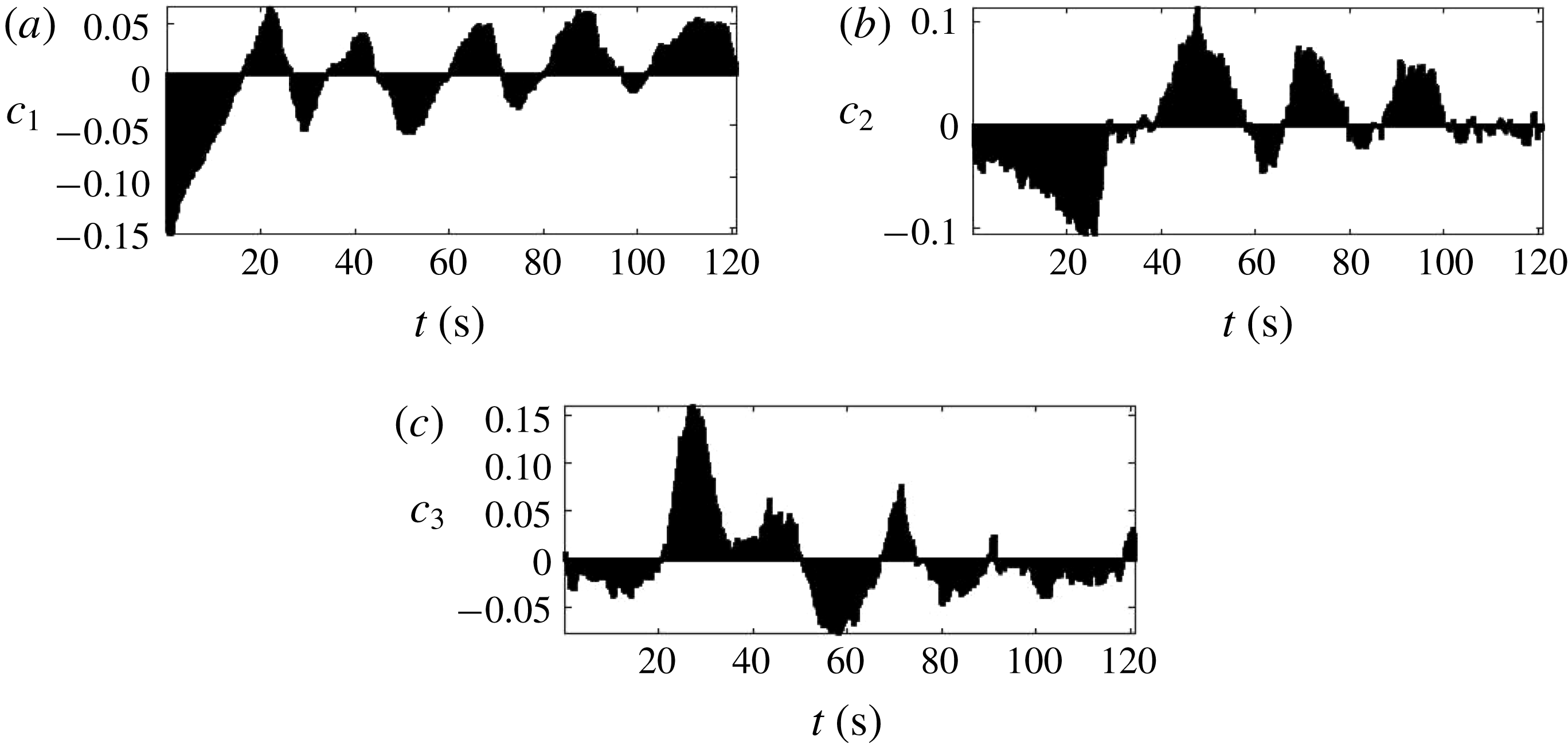
Figure 11. Time coefficient of (a) first, (b) second and (c) third POD mode in figure 10.

Figure 12. Fourier spectra for the time coefficient,
 $c_{1}(t)$
, of the first POD mode for a jet with
$c_{1}(t)$
, of the first POD mode for a jet with
 $Re_{0}=2300$
for four different rotation rates: (a)
$Re_{0}=2300$
for four different rotation rates: (a)
 $\unicode[STIX]{x1D6FA}=0.21~\text{rad}~\text{s}^{-1}$
, (b)
$\unicode[STIX]{x1D6FA}=0.21~\text{rad}~\text{s}^{-1}$
, (b)
 $\unicode[STIX]{x1D6FA}=0.41~\text{rad}~\text{s}^{-1}$
, (c)
$\unicode[STIX]{x1D6FA}=0.41~\text{rad}~\text{s}^{-1}$
, (c)
 $\unicode[STIX]{x1D6FA}=0.73~\text{rad}~\text{s}^{-1}$
and (d)
$\unicode[STIX]{x1D6FA}=0.73~\text{rad}~\text{s}^{-1}$
and (d)
 $\unicode[STIX]{x1D6FA}=1.05~\text{rad}~\text{s}^{-1}$
.
$\unicode[STIX]{x1D6FA}=1.05~\text{rad}~\text{s}^{-1}$
.
Subjecting the time coefficient
 $c_{1}(t)$
of the first POD mode, i.e. the energetically dominant mode, to a Fourier analysis yields the repetition frequency,
$c_{1}(t)$
of the first POD mode, i.e. the energetically dominant mode, to a Fourier analysis yields the repetition frequency,
 $f_{\unicode[STIX]{x1D703}}$
, associated with the formation–breakdown scenario of the jet structure. Figure 12 displays the Fourier spectra for
$f_{\unicode[STIX]{x1D703}}$
, associated with the formation–breakdown scenario of the jet structure. Figure 12 displays the Fourier spectra for
 $c_{1}(t)$
for experiments with four different background rotation rates. For each spectrum of figure 12(a–d) the dominant peak identifies
$c_{1}(t)$
for experiments with four different background rotation rates. For each spectrum of figure 12(a–d) the dominant peak identifies
 $f_{\unicode[STIX]{x1D703}}$
for each of the four associated rotational speeds of the turntable.
$f_{\unicode[STIX]{x1D703}}$
for each of the four associated rotational speeds of the turntable.
Figure 13 displays the summary of all available data for
 $f_{\unicode[STIX]{x1D703}}$
as a function of the frequency,
$f_{\unicode[STIX]{x1D703}}$
as a function of the frequency,
 $f_{T}=\unicode[STIX]{x1D6FA}/2\unicode[STIX]{x03C0}$
, of the background rotation of the turntable and for two different values
$f_{T}=\unicode[STIX]{x1D6FA}/2\unicode[STIX]{x03C0}$
, of the background rotation of the turntable and for two different values
 $Re_{0}=2300$
and
$Re_{0}=2300$
and
 $Re_{0}=16\,000$
of the jet Reynolds number. Figure 13 reveals that
$Re_{0}=16\,000$
of the jet Reynolds number. Figure 13 reveals that
 $f_{\unicode[STIX]{x1D703}}$
increases approximately linearly with
$f_{\unicode[STIX]{x1D703}}$
increases approximately linearly with
 $f_{T}$
within the explored range of
$f_{T}$
within the explored range of
 $0.067~\text{Hz}\leqslant f_{T}\leqslant 0.17~\text{Hz}$
(corresponding to the range 2–10 r.p.m.) for both Reynolds numbers. Figure 13 moreover shows that the formation–breakdown frequency also increases with the Reynolds number.
$0.067~\text{Hz}\leqslant f_{T}\leqslant 0.17~\text{Hz}$
(corresponding to the range 2–10 r.p.m.) for both Reynolds numbers. Figure 13 moreover shows that the formation–breakdown frequency also increases with the Reynolds number.
The linear least-squares interpolations of the data points in figure 13 are given by
 $f_{\unicode[STIX]{x1D703}}=0.83f_{T}$
for
$f_{\unicode[STIX]{x1D703}}=0.83f_{T}$
for
 $Re_{0}=2300$
and
$Re_{0}=2300$
and
 $f_{\unicode[STIX]{x1D703}}=1.61f_{T}$
for
$f_{\unicode[STIX]{x1D703}}=1.61f_{T}$
for
 $Re_{0}=16\,000$
. This implies that the measured ratio of formation–breakdown frequency and the frequency of the table rotation is in the range
$Re_{0}=16\,000$
. This implies that the measured ratio of formation–breakdown frequency and the frequency of the table rotation is in the range
 $0.83\leqslant f_{\unicode[STIX]{x1D703}}/f_{T}\leqslant 1.61$
for
$0.83\leqslant f_{\unicode[STIX]{x1D703}}/f_{T}\leqslant 1.61$
for
 $2300\leqslant Re_{0}\leqslant 16\,000$
. Note that the range obtained for
$2300\leqslant Re_{0}\leqslant 16\,000$
. Note that the range obtained for
 $f_{\unicode[STIX]{x1D703}}/f_{T}$
is similar to the value of
$f_{\unicode[STIX]{x1D703}}/f_{T}$
is similar to the value of
 $f_{\unicode[STIX]{x1D703}}/f_{T}\approx 2$
one infers from the information provided in the abstract of Niino (Reference Niino1980) for the residual damped oscillations that his inviscid theory predicts to exist near the forcing region – when consulting the paper by Niino note that he uses
$f_{\unicode[STIX]{x1D703}}/f_{T}\approx 2$
one infers from the information provided in the abstract of Niino (Reference Niino1980) for the residual damped oscillations that his inviscid theory predicts to exist near the forcing region – when consulting the paper by Niino note that he uses
 $f$
to refer to the Coriolis parameter,
$f$
to refer to the Coriolis parameter,
 $2\unicode[STIX]{x1D6FA}$
. However, the data available do not allow one to establish whether this similarity of the values is coincidental.
$2\unicode[STIX]{x1D6FA}$
. However, the data available do not allow one to establish whether this similarity of the values is coincidental.

Figure 13. Formation–breakdown frequency,
 $f_{\unicode[STIX]{x1D703}}$
, of the jets as a function of the background rotation frequency,
$f_{\unicode[STIX]{x1D703}}$
, of the jets as a function of the background rotation frequency,
 $f_{T}=\unicode[STIX]{x1D6FA}/2\unicode[STIX]{x03C0}$
, of the turntable.
$f_{T}=\unicode[STIX]{x1D6FA}/2\unicode[STIX]{x03C0}$
, of the turntable.

Figure 14. Variation of formation–breakdown frequency,
 $f_{\unicode[STIX]{x1D703}}$
, of the jets as a function of the Reynolds number
$f_{\unicode[STIX]{x1D703}}$
, of the jets as a function of the Reynolds number
 $Re_{0}$
at
$Re_{0}$
at
 $f_{T}=0.033$
(
$f_{T}=0.033$
(
 $\unicode[STIX]{x1D6FA}=0.21~\text{rad}~\text{s}^{-1}$
).
$\unicode[STIX]{x1D6FA}=0.21~\text{rad}~\text{s}^{-1}$
).
Figure 14 shows the dependence of the formation–breakdown frequency on the Reynolds number
 $Re_{0}$
for three different rotation rates,
$Re_{0}$
for three different rotation rates,
 $\unicode[STIX]{x1D6FA}=0.21~\text{rad}~\text{s}^{-1}$
,
$\unicode[STIX]{x1D6FA}=0.21~\text{rad}~\text{s}^{-1}$
,
 $\unicode[STIX]{x1D6FA}=0.52~\text{rad}~\text{s}^{-1}$
and
$\unicode[STIX]{x1D6FA}=0.52~\text{rad}~\text{s}^{-1}$
and
 $\unicode[STIX]{x1D6FA}=1.05~\text{rad}~\text{s}^{-1}$
, corresponding to
$\unicode[STIX]{x1D6FA}=1.05~\text{rad}~\text{s}^{-1}$
, corresponding to
 $f_{T}=0.033$
,
$f_{T}=0.033$
,
 $f_{T}=0.083$
and
$f_{T}=0.083$
and
 $f_{T}=0.167$
, respectively. Since the diameter of the source was not varied, the increase of the Reynolds number reflects increasing fluid ejection rates at the source. In addition to the results of figure 13, figure 14 reveals that
$f_{T}=0.167$
, respectively. Since the diameter of the source was not varied, the increase of the Reynolds number reflects increasing fluid ejection rates at the source. In addition to the results of figure 13, figure 14 reveals that
 $f_{\unicode[STIX]{x1D703}}$
increases approximately linearly with
$f_{\unicode[STIX]{x1D703}}$
increases approximately linearly with
 $Re_{0}$
for the regime of Reynolds numbers explored.
$Re_{0}$
for the regime of Reynolds numbers explored.
4.3.2 Radial velocity profiles of the azimuthal velocity component
The main goal of this section is to determine the temporal variation of the radial profile of the azimuthal velocity component,
 $v_{\unicode[STIX]{x1D703}}(r,t)$
, to use these results in § 4.3.2.5 for the definition of a local Rossby number which will be found to characterize the onset of the jet breakdown and the onset of its reformation process. As a consistency check, we will, moreover, reconfirm the main result of the POD analysis of figure 13 that the frequency of the formation–breakdown cycle scales linearly with the frequency of the table rotation. This consistency check will be facilitated through an analysis of the temporal variation of the kinetic energy associated with the azimuthal component of the flow velocity. This variation of the kinetic energy can be characterized by evaluating
$v_{\unicode[STIX]{x1D703}}(r,t)$
, to use these results in § 4.3.2.5 for the definition of a local Rossby number which will be found to characterize the onset of the jet breakdown and the onset of its reformation process. As a consistency check, we will, moreover, reconfirm the main result of the POD analysis of figure 13 that the frequency of the formation–breakdown cycle scales linearly with the frequency of the table rotation. This consistency check will be facilitated through an analysis of the temporal variation of the kinetic energy associated with the azimuthal component of the flow velocity. This variation of the kinetic energy can be characterized by evaluating
 $$\begin{eqnarray}E_{\unicode[STIX]{x1D703}}(t)=\int _{0}^{R}v_{\unicode[STIX]{x1D703}}^{2}(r,t)r\,\text{d}r\end{eqnarray}$$
for successive PIV frames. This also requires the availability of profiles
 $v_{\unicode[STIX]{x1D703}}(r,t)$
of the swirling flow. However, determining the velocity profiles requires, in turn, a definition of what constitutes the centre of the swirling flow field. Once the profiles
$v_{\unicode[STIX]{x1D703}}(r,t)$
of the swirling flow. However, determining the velocity profiles requires, in turn, a definition of what constitutes the centre of the swirling flow field. Once the profiles
 $v_{\unicode[STIX]{x1D703}}(r,t)$
are known, one can use these to define the necessary cutoff distance
$v_{\unicode[STIX]{x1D703}}(r,t)$
are known, one can use these to define the necessary cutoff distance
 $R$
to calculate (4.1). Since the flow field displays phases of more or less regular axisymmetric circular swirl and irregular flow phases during the formation–breakdown cycle, we will determine circumferentially averaged velocity profiles,
$R$
to calculate (4.1). Since the flow field displays phases of more or less regular axisymmetric circular swirl and irregular flow phases during the formation–breakdown cycle, we will determine circumferentially averaged velocity profiles,
 $\overline{v}_{\unicode[STIX]{x1D703}}(r,t)$
, and use these to evaluate (4.1).
$\overline{v}_{\unicode[STIX]{x1D703}}(r,t)$
, and use these to evaluate (4.1).
4.3.2.1 Identification of the centre of the swirling flow field
In order to identify the centre of the swirling flow structure on the measurement domain, we followed Graftieaux, Michard & Grosjean (Reference Graftieaux, Michard and Grosjean2001) whose method proceeds as follows. Let
 $S$
refer to the 2D, discrete, rectangular PIV measurement domain containing
$S$
refer to the 2D, discrete, rectangular PIV measurement domain containing
 $N$
pixel sites. Aligned perpendicular to this domain is the unit vector
$N$
pixel sites. Aligned perpendicular to this domain is the unit vector
 $\boldsymbol{e}_{z}$
in the direction of the
$\boldsymbol{e}_{z}$
in the direction of the
 $z$
-axis. Let
$z$
-axis. Let
 $P$
refer to the particular pixel site upon which
$P$
refer to the particular pixel site upon which
 $S$
is centred and denote the remaining locations on the measurement domain as
$S$
is centred and denote the remaining locations on the measurement domain as
 $M$
. Let
$M$
. Let
 $\boldsymbol{a}$
be the radius vector from
$\boldsymbol{a}$
be the radius vector from
 $P$
to
$P$
to
 $M$
, let
$M$
, let
 $\boldsymbol{U}_{M}$
denote the velocity vector at
$\boldsymbol{U}_{M}$
denote the velocity vector at
 $M$
and let
$M$
and let
 $\unicode[STIX]{x1D719}_{M}$
represent the angle between
$\unicode[STIX]{x1D719}_{M}$
represent the angle between
 $\boldsymbol{a}$
and
$\boldsymbol{a}$
and
 $\boldsymbol{U}_{M}$
. Graftieaux et al. (Reference Graftieaux, Michard and Grosjean2001) initially consider a dimensionless scalar function
$\boldsymbol{U}_{M}$
. Graftieaux et al. (Reference Graftieaux, Michard and Grosjean2001) initially consider a dimensionless scalar function
 $\unicode[STIX]{x1D6E4}_{1}(P)$
obtained by integration over a continuous domain
$\unicode[STIX]{x1D6E4}_{1}(P)$
obtained by integration over a continuous domain
 $D$
. However, for the discrete spatial PIV measurement domain, this integral relation reduces to
$D$
. However, for the discrete spatial PIV measurement domain, this integral relation reduces to
 $$\begin{eqnarray}\unicode[STIX]{x1D6E4}_{1}(P)=\frac{1}{N}\mathop{\sum }_{D}\frac{(\boldsymbol{a}\times \boldsymbol{U}_{M})\boldsymbol{\cdot }\boldsymbol{e}_{z}}{|\boldsymbol{a}|\,|\boldsymbol{U}_{M}|}=\frac{1}{N}\mathop{\sum }_{D}\sin (\unicode[STIX]{x1D719}_{M}).\end{eqnarray}$$
Thus,
 $\unicode[STIX]{x1D6E4}_{1}$
is a dimensionless scalar, with
$\unicode[STIX]{x1D6E4}_{1}$
is a dimensionless scalar, with
 $|\unicode[STIX]{x1D6E4}_{1}|\leqslant 1$
. If the centre of an idealized, perfectly circular vortex centre was located at
$|\unicode[STIX]{x1D6E4}_{1}|\leqslant 1$
. If the centre of an idealized, perfectly circular vortex centre was located at
 $P$
, then
$P$
, then
 $\boldsymbol{U}_{M}$
would be perpendicular to
$\boldsymbol{U}_{M}$
would be perpendicular to
 $\boldsymbol{a}$
at all pixel sites. This implies that
$\boldsymbol{a}$
at all pixel sites. This implies that
 $\sin \unicode[STIX]{x1D719}_{M}=1$
at all pixel sites and it follows, therewith, that
$\sin \unicode[STIX]{x1D719}_{M}=1$
at all pixel sites and it follows, therewith, that
 $\unicode[STIX]{x1D6E4}_{1}(P)$
adopts its maximum value at
$\unicode[STIX]{x1D6E4}_{1}(P)$
adopts its maximum value at
 $P$
. Consequently, the strategy for identifying the vortex structure in the measurement domain is to determine the value of
$P$
. Consequently, the strategy for identifying the vortex structure in the measurement domain is to determine the value of
 $\unicode[STIX]{x1D6E4}_{1}$
for all pixel sites and find that particular site with the largest value for this parameter. Graftieaux et al. (Reference Graftieaux, Michard and Grosjean2001) state that
$\unicode[STIX]{x1D6E4}_{1}$
for all pixel sites and find that particular site with the largest value for this parameter. Graftieaux et al. (Reference Graftieaux, Michard and Grosjean2001) state that
 $\unicode[STIX]{x1D6E4}_{1}$
typically reaches values from
$\unicode[STIX]{x1D6E4}_{1}$
typically reaches values from
 $0.9$
to
$0.9$
to
 $1$
near the vortex centre, independent of the value of
$1$
near the vortex centre, independent of the value of
 $N$
– the current observations are consistent with this. Graftieaux et al. (Reference Graftieaux, Michard and Grosjean2001) discuss, moreover, that
$N$
– the current observations are consistent with this. Graftieaux et al. (Reference Graftieaux, Michard and Grosjean2001) discuss, moreover, that
 $N$
plays the role of a spatial filter and it is therewith possible to remove small-scale turbulent fluctuations through the selection of the particular value of
$N$
plays the role of a spatial filter and it is therewith possible to remove small-scale turbulent fluctuations through the selection of the particular value of
 $N$
to be used.
$N$
to be used.

Figure 15. Two examples illustrating the performance of the centre-finding process of Graftieaux et al. (Reference Graftieaux, Michard and Grosjean2001) applied to flow fields from the current experiments for
 $Re_{0}=2300$
, at
$Re_{0}=2300$
, at
 $\unicode[STIX]{x1D6FA}=0.21~\text{rad}~\text{s}^{-1}$
, with (a)
$\unicode[STIX]{x1D6FA}=0.21~\text{rad}~\text{s}^{-1}$
, with (a)
 $\unicode[STIX]{x1D6E4}=0.87$
and (b)
$\unicode[STIX]{x1D6E4}=0.87$
and (b)
 $\unicode[STIX]{x1D6E4}=0.66$
. Centres are identified in both plots through a bold black cross.
$\unicode[STIX]{x1D6E4}=0.66$
. Centres are identified in both plots through a bold black cross.
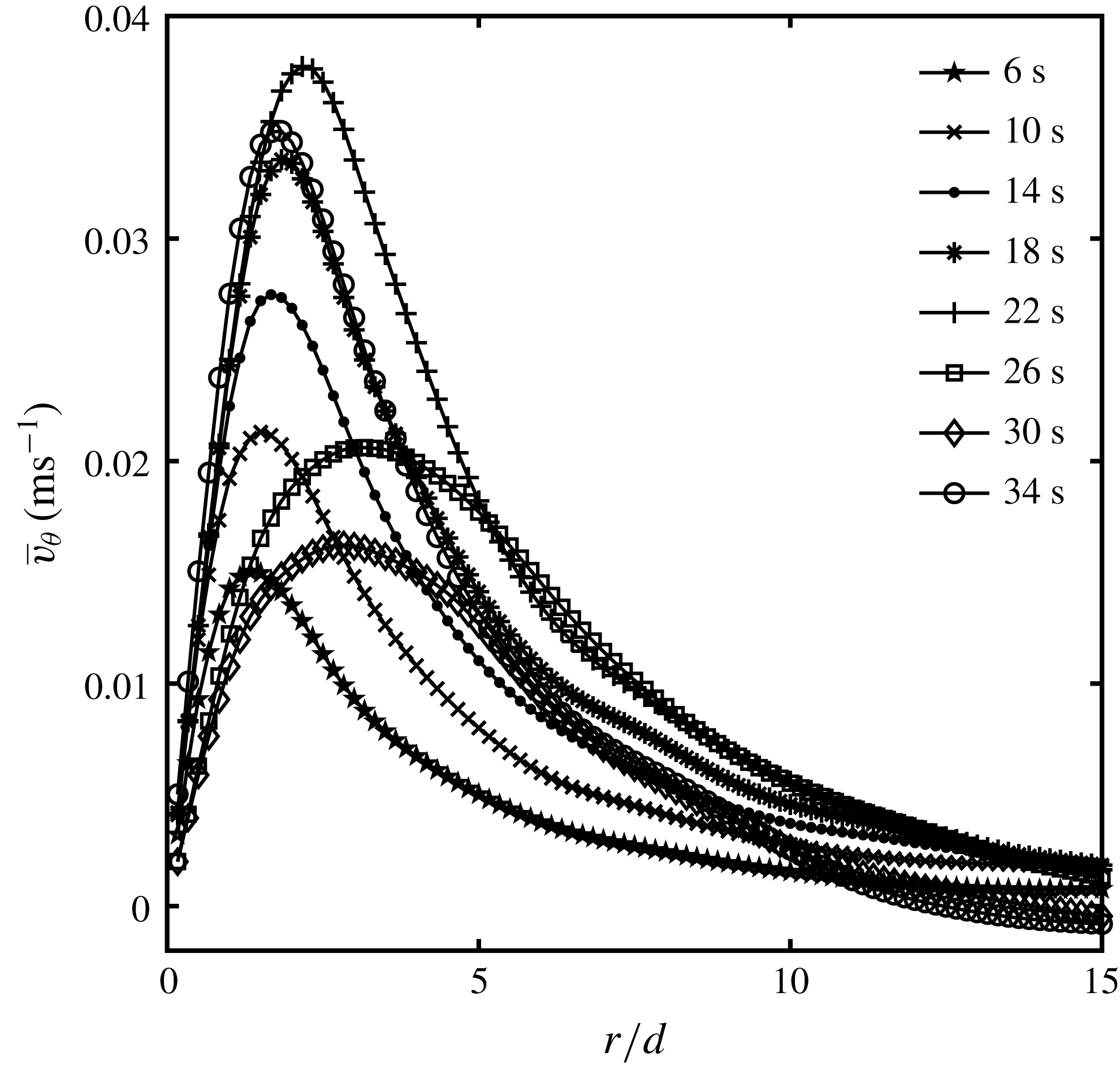
Figure 16. Profiles of the circumferentially averaged azimuthal velocity component
 $\overline{v}_{\unicode[STIX]{x1D703}}$
as a function of the distance
$\overline{v}_{\unicode[STIX]{x1D703}}$
as a function of the distance
 $r/d$
from the centre for different instants in time.
$r/d$
from the centre for different instants in time.
Figure 15 displays examples of two PIV flow-field frames on which the centre, as identified by the centre-finding process of Graftieaux et al. (Reference Graftieaux, Michard and Grosjean2001), is marked by a bold black cross. In figure 15 vorticity is identified through the colour bar and the magnitude of the velocity is characterized by the lengths of the velocity vectors. The inspection of the symmetric flow field in figure 15(a) reveals that the location of the centre of the flow structure corresponds well with the position one would have intuitively chosen, based on a visual inspection only. However, when the flow field is more complex and less symmetric, as is the case during later stages of the formation–decay cycle of the jet, a centre location by visual inspection is, evidently, not that straightforward, as is illustrated by considering figure 15(b). Further, more quantitative, evidence in support of the good performance of the centre-finding algorithm will be presented in § 4.3.2.2 where the circumferentially averaged azimuthal velocity component
 $\overline{v}_{\unicode[STIX]{x1D703}}$
is calculated.
$\overline{v}_{\unicode[STIX]{x1D703}}$
is calculated.
4.3.2.2 Velocity profiles
Figure 16 displays a series of profiles of the circumferentially averaged, azimuthal velocity component,
 $\overline{v}_{\unicode[STIX]{x1D703}}(r,t)$
, as a function of the radial position
$\overline{v}_{\unicode[STIX]{x1D703}}(r,t)$
, as a function of the radial position
 $r/d$
at height
$r/d$
at height
 $z/d=0.5$
above the source. These profiles were determined from the PIV data on the basis of the centre of the flow field determined as described in § 4.3.2.1. Figure 16 shows eight datasets spanning a total interval of 34 s during a formation–breakdown cycle of a jet with
$z/d=0.5$
above the source. These profiles were determined from the PIV data on the basis of the centre of the flow field determined as described in § 4.3.2.1. Figure 16 shows eight datasets spanning a total interval of 34 s during a formation–breakdown cycle of a jet with
 $Re_{0}=2300$
at
$Re_{0}=2300$
at
 $\unicode[STIX]{x1D6FA}=0.21~\text{rad}~\text{s}^{-1}$
. Corresponding to the procedures employed for the POD analysis in § 4.3.1, the vector fields determined from the PIV measurements were acquired at a rate of 90 frames per second and then averaged over successive periods of
$\unicode[STIX]{x1D6FA}=0.21~\text{rad}~\text{s}^{-1}$
. Corresponding to the procedures employed for the POD analysis in § 4.3.1, the vector fields determined from the PIV measurements were acquired at a rate of 90 frames per second and then averaged over successive periods of
 $\unicode[STIX]{x0394}t=0.25~\text{s}$
before calculating the circumferentially averaged velocity
$\unicode[STIX]{x0394}t=0.25~\text{s}$
before calculating the circumferentially averaged velocity
 $\overline{v}_{\unicode[STIX]{x1D703}}$
.
$\overline{v}_{\unicode[STIX]{x1D703}}$
.
Figure 16 reveals, firstly, that for
 $r/d\rightarrow 0$
the profiles for all times satisfy the expected condition
$r/d\rightarrow 0$
the profiles for all times satisfy the expected condition
 $\overline{v}_{\unicode[STIX]{x1D703}}\rightarrow 0$
. This represents quantitative evidence for a good performance of the process described in § 4.3.2.1 to identify the centre of the flow field. Data from profiles such as those in figure 16 will be used in § 4.3.2.5 to define a local Rossby number and determine critical values for this parameter that characterize the onset of the jet breakdown and the onset of its reformation process.
$\overline{v}_{\unicode[STIX]{x1D703}}\rightarrow 0$
. This represents quantitative evidence for a good performance of the process described in § 4.3.2.1 to identify the centre of the flow field. Data from profiles such as those in figure 16 will be used in § 4.3.2.5 to define a local Rossby number and determine critical values for this parameter that characterize the onset of the jet breakdown and the onset of its reformation process.
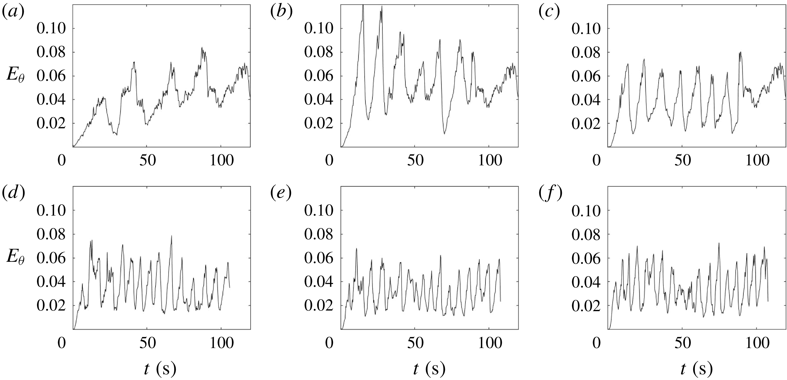
Figure 17. Temporal variation of the kinetic energy associated with azimuthal velocity component, at
 $Re_{0}=2300$
, for six different rotation rates, in units
$Re_{0}=2300$
, for six different rotation rates, in units
 $\text{rad}~\text{s}^{-1}$
: (a)
$\text{rad}~\text{s}^{-1}$
: (a)
 $0.21$
, (b)
$0.21$
, (b)
 $0.31$
, (c)
$0.31$
, (c)
 $0.42$
, (d)
$0.42$
, (d)
 $0.84$
, (e)
$0.84$
, (e)
 $0.94$
and (f)
$0.94$
and (f)
 $1.05$
.
$1.05$
.
4.3.2.3 Cutoff radius
The evaluation of the temporal variation of kinetic energy associated with the azimuthal flow velocity, by means of (4.1), requires the cutoff value for the radial extent
 $R$
to be defined. Figure 16 demonstrates that the azimuthal flow velocity approaches values
$R$
to be defined. Figure 16 demonstrates that the azimuthal flow velocity approaches values
 $\overline{v}_{\unicode[STIX]{x1D703}}\approx 0$
, for all profiles displayed, for radial locations
$\overline{v}_{\unicode[STIX]{x1D703}}\approx 0$
, for all profiles displayed, for radial locations
 $r/d\gtrsim 10$
. Therefore we have selected
$r/d\gtrsim 10$
. Therefore we have selected
 $r/d=15$
as the cutoff location such that
$r/d=15$
as the cutoff location such that
 $R=15d$
in (4.1). The precise choice for the value for
$R=15d$
in (4.1). The precise choice for the value for
 $R$
will not strongly affect the value of (4.1) as long as the bulk of the kinetic energy is captured by the integral – which is certainly the case for any choice of the cutoff value with
$R$
will not strongly affect the value of (4.1) as long as the bulk of the kinetic energy is captured by the integral – which is certainly the case for any choice of the cutoff value with
 $r/d\gtrsim 10$
.
$r/d\gtrsim 10$
.
4.3.2.4 Analysis of the kinetic energy associated with the azimuthal flow component
The velocity profiles
 $\overline{v}_{\unicode[STIX]{x1D703}}(r,t)$
and the cutoff radius,
$\overline{v}_{\unicode[STIX]{x1D703}}(r,t)$
and the cutoff radius,
 $R$
, are now known and it is therefore possible to calculate (4.1) on the flow domain to evaluate and analyse the temporal variation of
$R$
, are now known and it is therefore possible to calculate (4.1) on the flow domain to evaluate and analyse the temporal variation of
 $E_{\unicode[STIX]{x1D703}}(t)$
to perform a consistency check reconfirming the results obtained in figure 13 from the POD analysis.
$E_{\unicode[STIX]{x1D703}}(t)$
to perform a consistency check reconfirming the results obtained in figure 13 from the POD analysis.
Figure 17 illustrates samples for the temporal variation of
 $E_{\unicode[STIX]{x1D703}}(t)$
for a jet with
$E_{\unicode[STIX]{x1D703}}(t)$
for a jet with
 $Re_{0}=2300$
at six different rotation rates. It can be seen that all the panels display very regular fluctuations of
$Re_{0}=2300$
at six different rotation rates. It can be seen that all the panels display very regular fluctuations of
 $E_{\unicode[STIX]{x1D703}}(t)$
for all rotation rates. Comparison of the panels in figure 17 moreover reveals, qualitatively, that the formation–breakdown frequency
$E_{\unicode[STIX]{x1D703}}(t)$
for all rotation rates. Comparison of the panels in figure 17 moreover reveals, qualitatively, that the formation–breakdown frequency
 $f_{\unicode[STIX]{x1D703}}$
increases with increasing values of the background rotation.
$f_{\unicode[STIX]{x1D703}}$
increases with increasing values of the background rotation.

Figure 18. Fourier spectra for the temporal variation of the kinetic energy associated with azimuthal velocity components,
 $Re_{0}=2300$
, for six different rotation rates, in units
$Re_{0}=2300$
, for six different rotation rates, in units
 $\text{rad}~\text{s}^{-1}$
: (a)
$\text{rad}~\text{s}^{-1}$
: (a)
 $0.21$
, (b)
$0.21$
, (b)
 $0.31$
, (c)
$0.31$
, (c)
 $0.42$
, (d)
$0.42$
, (d)
 $0.84$
, (e)
$0.84$
, (e)
 $0.94$
and (f)
$0.94$
and (f)
 $1.05$
.
$1.05$
.

Figure 19. Formation–breakdown frequency,
 $f_{\unicode[STIX]{x1D703}}$
, of the jets as a function of the background rotation frequency,
$f_{\unicode[STIX]{x1D703}}$
, of the jets as a function of the background rotation frequency,
 $f_{T}=\unicode[STIX]{x1D6FA}/2\unicode[STIX]{x03C0}$
, of the turntable:
$f_{T}=\unicode[STIX]{x1D6FA}/2\unicode[STIX]{x03C0}$
, of the turntable:
 $\ast$
, ——,
$\ast$
, ——,
 $Re_{0}=2300$
,
$Re_{0}=2300$
,
 $f_{\unicode[STIX]{x1D703}}=0.84f_{T}$
; ○, – – –,
$f_{\unicode[STIX]{x1D703}}=0.84f_{T}$
; ○, – – –,
 $Re_{0}=16\,000$
,
$Re_{0}=16\,000$
,
 $f_{\unicode[STIX]{x1D703}}=1.57f_{T}$
. The dotted lines in the immediate vicinity of the two least-squares interpolations are the corresponding data interpolations from figure 13 obtained in § 4.3.1 from the POD analysis.
$f_{\unicode[STIX]{x1D703}}=1.57f_{T}$
. The dotted lines in the immediate vicinity of the two least-squares interpolations are the corresponding data interpolations from figure 13 obtained in § 4.3.1 from the POD analysis.
The six Fourier spectra associated with the data for
 $E_{\unicode[STIX]{x1D703}}(t)$
in figure 17 are displayed in figure 18. In order to prevent data bias due to spectral leakage, we have multiplied each of the six data windows of figure 17 by a taper before performing the Fourier analysis. The formation–breakdown frequency
$E_{\unicode[STIX]{x1D703}}(t)$
in figure 17 are displayed in figure 18. In order to prevent data bias due to spectral leakage, we have multiplied each of the six data windows of figure 17 by a taper before performing the Fourier analysis. The formation–breakdown frequency
 $f_{\unicode[STIX]{x1D703}}$
is associated with the dominant peak in the spectra in figure 18. The frequencies for these peaks, for jets at
$f_{\unicode[STIX]{x1D703}}$
is associated with the dominant peak in the spectra in figure 18. The frequencies for these peaks, for jets at
 $Re_{0}=2300$
and
$Re_{0}=2300$
and
 $Re_{0}=16\,000$
, at different rotational frequencies
$Re_{0}=16\,000$
, at different rotational frequencies
 $f_{T}$
, are displayed in figure 19. The two least-squares interpolations of the two datasets for
$f_{T}$
, are displayed in figure 19. The two least-squares interpolations of the two datasets for
 $Re_{0}=2300$
and
$Re_{0}=2300$
and
 $Re_{0}=16\,000$
are given by, respectively,
$Re_{0}=16\,000$
are given by, respectively,
 $f_{\unicode[STIX]{x1D703}}=0.84f_{T}$
and
$f_{\unicode[STIX]{x1D703}}=0.84f_{T}$
and
 $f_{\unicode[STIX]{x1D703}}=1.57f_{T}$
and they are identified by the solid line and the dashed line, respectively. The superposed dotted lines shown in very close proximity of each one of these two least-squares data interpolations represent the corresponding interpolations obtained in § 4.3.1, in figure 13, from the analysis of the time coefficient of the first POD mode. Figure 19 reveals that, at both Reynolds numbers, the results from the POD analysis and from the analysis of the azimuthal kinetic energy are in very good quantitative agreement.
$f_{\unicode[STIX]{x1D703}}=1.57f_{T}$
and they are identified by the solid line and the dashed line, respectively. The superposed dotted lines shown in very close proximity of each one of these two least-squares data interpolations represent the corresponding interpolations obtained in § 4.3.1, in figure 13, from the analysis of the time coefficient of the first POD mode. Figure 19 reveals that, at both Reynolds numbers, the results from the POD analysis and from the analysis of the azimuthal kinetic energy are in very good quantitative agreement.
4.3.2.5 Local Rossby number variation
In § 2 the ejection Rossby number
 $Ro_{0}=u_{0}/\unicode[STIX]{x1D6FA}d$
was defined based on the mean ejection velocity and the nozzle diameter and this yielded values
$Ro_{0}=u_{0}/\unicode[STIX]{x1D6FA}d$
was defined based on the mean ejection velocity and the nozzle diameter and this yielded values
 $46\leqslant Ro_{0}\leqslant 2100$
. However, it is reasonable to assume that the dynamics of the jets, at any particular given height above the source, depends on a local velocity scale and a local length scale and that the global value
$46\leqslant Ro_{0}\leqslant 2100$
. However, it is reasonable to assume that the dynamics of the jets, at any particular given height above the source, depends on a local velocity scale and a local length scale and that the global value
 $Ro_{0}$
is not the most appropriate, and dynamically relevant, definition for the Rossby number. The analysis of our PIV measurements yielded data for the circumferentially averaged profiles of the azimuthal velocity component (cf. figure 16) throughout the formation–decay cycles of the jets. Therewith it is possible to calculate an alternative, dynamically more relevant, instantaneous, local Rossby number analogous to the definition used in Kloosterziel & van Heijst (Reference Kloosterziel and van Heijst1991) for vortices in a rotating fluid. This instantaneous, local Rossby number,
$Ro_{0}$
is not the most appropriate, and dynamically relevant, definition for the Rossby number. The analysis of our PIV measurements yielded data for the circumferentially averaged profiles of the azimuthal velocity component (cf. figure 16) throughout the formation–decay cycles of the jets. Therewith it is possible to calculate an alternative, dynamically more relevant, instantaneous, local Rossby number analogous to the definition used in Kloosterziel & van Heijst (Reference Kloosterziel and van Heijst1991) for vortices in a rotating fluid. This instantaneous, local Rossby number,
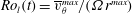 $Ro_{l}(t)=\overline{v}_{\unicode[STIX]{x1D703}}^{max}/(\unicode[STIX]{x1D6FA}r^{max})$
, is based on the radial location,
$Ro_{l}(t)=\overline{v}_{\unicode[STIX]{x1D703}}^{max}/(\unicode[STIX]{x1D6FA}r^{max})$
, is based on the radial location,
 $r^{max}(t)$
, where the velocity profiles in figure 16 reach their maximum and the maximum velocity value
$r^{max}(t)$
, where the velocity profiles in figure 16 reach their maximum and the maximum velocity value
 $\overline{v}_{\unicode[STIX]{x1D703}}^{max}(t)$
at this location.
$\overline{v}_{\unicode[STIX]{x1D703}}^{max}(t)$
at this location.

Figure 20. Variation of the instantaneous, local Rossby number,
 $Ro_{l}$
, with time, for a jet with
$Ro_{l}$
, with time, for a jet with
 $Re_{0}=2300$
at
$Re_{0}=2300$
at
 $\unicode[STIX]{x1D6FA}=1.05~\text{rad}~\text{s}^{-1}$
, corresponding to
$\unicode[STIX]{x1D6FA}=1.05~\text{rad}~\text{s}^{-1}$
, corresponding to
 $Ro_{0}=60$
, near source at
$Ro_{0}=60$
, near source at
 $z/d=0.5$
.
$z/d=0.5$
.

Figure 21. The mean values of the maximum and minimum local Rossby number,
 $Ro_{l}^{U}$
and
$Ro_{l}^{U}$
and
 $Ro_{l}^{L}$
, as a function of the global Rossby number,
$Ro_{l}^{L}$
, as a function of the global Rossby number,
 $Ro_{0}$
, at height
$Ro_{0}$
, at height
 $z/d=0.5$
above the source. For
$z/d=0.5$
above the source. For
 $Re_{0}=2300$
: upper limit, ▪, ——,
$Re_{0}=2300$
: upper limit, ▪, ——,
 $Ro_{l}^{U}=0.011Ro_{0}-4$
; lower limit, ▫, – – –,
$Ro_{l}^{U}=0.011Ro_{0}-4$
; lower limit, ▫, – – –,
 $Ro_{l}^{L}=0.05Ro_{0}-0.21$
. For
$Ro_{l}^{L}=0.05Ro_{0}-0.21$
. For
 $Re_{0}=16\,000,~Ro_{0}\leqslant 850$
: upper limit, ●, — ⋅ ⋅ —,
$Re_{0}=16\,000,~Ro_{0}\leqslant 850$
: upper limit, ●, — ⋅ ⋅ —,
 $Ro_{l}^{U}=0.0015Ro_{0}+2.27$
; lower limit, ○, –
$Ro_{l}^{U}=0.0015Ro_{0}+2.27$
; lower limit, ○, –
 $\cdot$
–
$\cdot$
–
 $\cdot$
,
$\cdot$
,
 $Ro_{l}^{L}=0.002Ro_{0}+0.27$
.
$Ro_{l}^{L}=0.002Ro_{0}+0.27$
.
The values of
 $Ro_{l}(t)$
must be expected to vary with the height
$Ro_{l}(t)$
must be expected to vary with the height
 $z$
above the source where the profiles of
$z$
above the source where the profiles of
 $\overline{v}_{\unicode[STIX]{x1D703}}(t)$
were measured. In order to characterize the jets, we will, therefore, consider the value of
$\overline{v}_{\unicode[STIX]{x1D703}}(t)$
were measured. In order to characterize the jets, we will, therefore, consider the value of
 $Ro_{l}(t)$
in the immediate vicinity of the source at
$Ro_{l}(t)$
in the immediate vicinity of the source at
 $z/d=0.5$
. Figure 20 displays the temporal variation of
$z/d=0.5$
. Figure 20 displays the temporal variation of
 $Ro_{l}(t)$
at this height for a jet with
$Ro_{l}(t)$
at this height for a jet with
 $Re_{0}=2300$
and
$Re_{0}=2300$
and
 $\unicode[STIX]{x1D6FA}=0.21~\text{rad}~\text{s}^{-1}$
, corresponding to
$\unicode[STIX]{x1D6FA}=0.21~\text{rad}~\text{s}^{-1}$
, corresponding to
 $Ro_{0}=302$
, throughout an interval of 100 s containing several formation–decay cycles. Figure 20 reveals that the local Rossby number displays temporal fluctuations within the range
$Ro_{0}=302$
, throughout an interval of 100 s containing several formation–decay cycles. Figure 20 reveals that the local Rossby number displays temporal fluctuations within the range
 $1\lesssim Ro_{l}(t)\lesssim 5$
. The maximum value of the local Rossby number in each fluctuation cycle corresponds to the critical value at which the jet begins to decay, while the minimum value in each cycle corresponds to that value where a new formation cycle is initiated. The mean of the maximum values of
$1\lesssim Ro_{l}(t)\lesssim 5$
. The maximum value of the local Rossby number in each fluctuation cycle corresponds to the critical value at which the jet begins to decay, while the minimum value in each cycle corresponds to that value where a new formation cycle is initiated. The mean of the maximum values of
 $Ro_{l}(t)$
yields a critical upper limit,
$Ro_{l}(t)$
yields a critical upper limit,
 $Ro_{l}^{U}$
, where jet decay is initiated, while the mean of the minimum values yields a critical lower limit,
$Ro_{l}^{U}$
, where jet decay is initiated, while the mean of the minimum values yields a critical lower limit,
 $Ro_{l}^{L}$
, when a new formation cycle is initiated.
$Ro_{l}^{L}$
, when a new formation cycle is initiated.
Figure 21 summarizes the available data for
 $Ro_{l}^{U}$
and
$Ro_{l}^{U}$
and
 $Ro_{l}^{L}$
at the two Reynolds numbers
$Ro_{l}^{L}$
at the two Reynolds numbers
 $Re_{0}=2300$
and
$Re_{0}=2300$
and
 $Re_{0}=16\,000$
over the associated ranges of values for the global Rossby number,
$Re_{0}=16\,000$
over the associated ranges of values for the global Rossby number,
 $Ro_{0}$
, for which experiments were conducted. The data for
$Ro_{0}$
, for which experiments were conducted. The data for
 $Re_{0}=2300$
are displayed as the squares at the lower end of the range of
$Re_{0}=2300$
are displayed as the squares at the lower end of the range of
 $Ro_{0}$
in figure 21, where
$Ro_{0}$
in figure 21, where
 $Ro_{l}^{U}$
corresponds to the black squares while
$Ro_{l}^{U}$
corresponds to the black squares while
 $Ro_{l}^{L}$
is identified by the open squares. Correspondingly the data for
$Ro_{l}^{L}$
is identified by the open squares. Correspondingly the data for
 $Re_{0}=16\,000$
are displayed as circles, where black circles identify
$Re_{0}=16\,000$
are displayed as circles, where black circles identify
 $Ro_{l}^{L}$
and open circles
$Ro_{l}^{L}$
and open circles
 $Ro_{l}^{U}$
. The lines interpolating the data for
$Ro_{l}^{U}$
. The lines interpolating the data for
 $Re_{0}=2300$
in figure 21 are linear least-squares fits given by
$Re_{0}=2300$
in figure 21 are linear least-squares fits given by
 $Ro_{l}^{U}=0.011Ro_{0}-4$
and
$Ro_{l}^{U}=0.011Ro_{0}-4$
and
 $Ro_{l}^{L}=0.05Ro_{0}-0.21$
. The additive constants for both these data interpolations are small, compared to
$Ro_{l}^{L}=0.05Ro_{0}-0.21$
. The additive constants for both these data interpolations are small, compared to
 $Ro_{l}^{U}$
and
$Ro_{l}^{U}$
and
 $Ro_{l}^{L}$
. Moreover, it is evidently required that both
$Ro_{l}^{L}$
. Moreover, it is evidently required that both
 $Ro_{l}^{U}$
and
$Ro_{l}^{U}$
and
 $Ro_{l}^{L}$
approach zero as
$Ro_{l}^{L}$
approach zero as
 $Ro_{0}\rightarrow 0$
, that is, when the ejection velocity
$Ro_{0}\rightarrow 0$
, that is, when the ejection velocity
 $u_{0}$
vanishes and when no jet exists. Consequently one can assume that the additive constants reflect measurement errors and, therefore, neglect them. Therewith one can conclude that
$u_{0}$
vanishes and when no jet exists. Consequently one can assume that the additive constants reflect measurement errors and, therefore, neglect them. Therewith one can conclude that
 $Ro_{l}^{U}\propto \unicode[STIX]{x1D6FA}^{-1}$
and
$Ro_{l}^{U}\propto \unicode[STIX]{x1D6FA}^{-1}$
and
 $Ro_{l}^{L}\propto \unicode[STIX]{x1D6FA}^{-1}$
.
$Ro_{l}^{L}\propto \unicode[STIX]{x1D6FA}^{-1}$
.
Note that the linear scaling of
 $Ro_{l}^{L}$
and
$Ro_{l}^{L}$
and
 $Ro_{l}^{U}$
with
$Ro_{l}^{U}$
with
 $Ro$
, at low values of the global Rossby number, also implies that in this regime the global Rossby number is sufficient to characterize the dynamic behaviour. Since
$Ro$
, at low values of the global Rossby number, also implies that in this regime the global Rossby number is sufficient to characterize the dynamic behaviour. Since
 $Ro_{l}$
for the type of jets studied here is currently difficult to measure, for most others this means that, depending on the exact circumstances, knowledge of the local Rossby number may not be required at lower Reynolds numbers.
$Ro_{l}$
for the type of jets studied here is currently difficult to measure, for most others this means that, depending on the exact circumstances, knowledge of the local Rossby number may not be required at lower Reynolds numbers.

Figure 22. Variation of
 $Ro_{l}$
with time, near the source at
$Ro_{l}$
with time, near the source at
 $z/d=0.5$
, for a jet with
$z/d=0.5$
, for a jet with
 $Re_{0}=16\,000$
:
$Re_{0}=16\,000$
:
 $\cdots \cdots$
,
$\cdots \cdots$
,
 $Ro_{0}=653$
,
$Ro_{0}=653$
,
 $\unicode[STIX]{x1D6FA}=0.42~\text{rad}~\text{s}^{-1}$
; ——,
$\unicode[STIX]{x1D6FA}=0.42~\text{rad}~\text{s}^{-1}$
; ——,
 $Ro_{0}=1055$
,
$Ro_{0}=1055$
,
 $\unicode[STIX]{x1D6FA}=0.73~\text{rad}~\text{s}^{-1}$
.
$\unicode[STIX]{x1D6FA}=0.73~\text{rad}~\text{s}^{-1}$
.
For jets at
 $Re_{0}=2300$
at all values of
$Re_{0}=2300$
at all values of
 $Ro_{0}$
, the fluctuations of
$Ro_{0}$
, the fluctuations of
 $Ro_{l}(t)$
look qualitatively very similar to the profile shown here in figure 20 for the particular value
$Ro_{l}(t)$
look qualitatively very similar to the profile shown here in figure 20 for the particular value
 $Ro_{0}=60$
. For all these experiments, it was straightforward to calculate critical mean values for
$Ro_{0}=60$
. For all these experiments, it was straightforward to calculate critical mean values for
 $Ro_{l}^{U}$
and
$Ro_{l}^{U}$
and
 $Ro_{l}^{L}$
as can be anticipated from the data structure in figure 20. However, at the higher Reynolds number
$Ro_{l}^{L}$
as can be anticipated from the data structure in figure 20. However, at the higher Reynolds number
 $Re_{0}=16\,000$
, the situation was different. Here the data for
$Re_{0}=16\,000$
, the situation was different. Here the data for
 $Ro_{l}(t)$
only look qualitatively similar to the curve in figure 20 for the three data points with the lowest values of
$Ro_{l}(t)$
only look qualitatively similar to the curve in figure 20 for the three data points with the lowest values of
 $Ro_{0}$
in figure 21. For the next three data points, up to
$Ro_{0}$
in figure 21. For the next three data points, up to
 $Ro_{0}=850$
the curves for
$Ro_{0}=850$
the curves for
 $Ro_{l}(t)$
resemble that curve identified in figure 22 by the dotted line for
$Ro_{l}(t)$
resemble that curve identified in figure 22 by the dotted line for
 $Ro_{0}=653$
. The temporal oscillations are still clearly identifiable but the values of the maxima and minima decrease somewhat for increasing time. For the remaining three experiments with
$Ro_{0}=653$
. The temporal oscillations are still clearly identifiable but the values of the maxima and minima decrease somewhat for increasing time. For the remaining three experiments with
 $Ro_{0}>850$
the behaviour of the time traces for
$Ro_{0}>850$
the behaviour of the time traces for
 $Ro_{l}(t)$
change fundamentally and resemble that illustrated by the solid line for
$Ro_{l}(t)$
change fundamentally and resemble that illustrated by the solid line for
 $Ro_{0}=1055$
in figure 22. Reference to the figure shows that a substantial increase of
$Ro_{0}=1055$
in figure 22. Reference to the figure shows that a substantial increase of
 $Ro_{l}(t)$
has occurred between the curve for
$Ro_{l}(t)$
has occurred between the curve for
 $Ro_{0}=653$
and
$Ro_{0}=653$
and
 $Ro_{0}=1055$
and, moreover, the temporal fluctuations also became significantly less well defined. We cannot provide a definitive explanation for this qualitative change in the flow behaviour other than speculate that it may be associated with developing turbulence at higher values of
$Ro_{0}=1055$
and, moreover, the temporal fluctuations also became significantly less well defined. We cannot provide a definitive explanation for this qualitative change in the flow behaviour other than speculate that it may be associated with developing turbulence at higher values of
 $Re_{0}$
and, concurrently, higher
$Re_{0}$
and, concurrently, higher
 $Ro_{0}$
. Nevertheless, the observation suggests that the values for
$Ro_{0}$
. Nevertheless, the observation suggests that the values for
 $Ro_{l}^{U}$
and
$Ro_{l}^{U}$
and
 $Ro_{l}^{L}$
above
$Ro_{l}^{L}$
above
 $Ro_{0}=850$
are substantially too high in comparison to the behaviour displayed by the data points for
$Ro_{0}=850$
are substantially too high in comparison to the behaviour displayed by the data points for
 $Re_{0}=16\,000$
at
$Re_{0}=16\,000$
at
 $Ro_{0}\leqslant 850$
. Therefore we have only performed linear least-squares data interpolations for the data with
$Ro_{0}\leqslant 850$
. Therefore we have only performed linear least-squares data interpolations for the data with
 $Ro_{0}\leqslant 850$
for the jets at
$Ro_{0}\leqslant 850$
for the jets at
 $Re_{0}=16\,000$
. These least-squares data interpolations are given by
$Re_{0}=16\,000$
. These least-squares data interpolations are given by
 $Ro_{l}^{U}=0.0015Ro_{0}+2.27$
and
$Ro_{l}^{U}=0.0015Ro_{0}+2.27$
and
 $Ro_{l}^{L}=0.002Ro_{0}+0.27$
. Note, however, that the gradients and the additive constants of these two data interpolations are somewhat affected by the temporal decrease of the maximum and minimum values, as displayed by the curve for
$Ro_{l}^{L}=0.002Ro_{0}+0.27$
. Note, however, that the gradients and the additive constants of these two data interpolations are somewhat affected by the temporal decrease of the maximum and minimum values, as displayed by the curve for
 $Ro_{0}=653$
in figure 22, for the three experiments at, and just below,
$Ro_{0}=653$
in figure 22, for the three experiments at, and just below,
 $Ro_{0}=850$
. For
$Ro_{0}=850$
. For
 $Ro_{0}>850$
the line segments in figure 21 simply connect the remaining points of the data for the jets at
$Ro_{0}>850$
the line segments in figure 21 simply connect the remaining points of the data for the jets at
 $Re_{0}=16\,000$
.
$Re_{0}=16\,000$
.
In summary, from the data displayed in figure 21, it can be concluded that the onset of the decay process of the jets, as well as the onset of their reformation process, are characterized by the local Rossby number
 $Ro_{l}$
. For global Rossby numbers
$Ro_{l}$
. For global Rossby numbers
 $Ro_{0}\leqslant 850$
the critical maximum upper local Rossby number,
$Ro_{0}\leqslant 850$
the critical maximum upper local Rossby number,
 $Ro_{l}^{U}$
, where decay is triggered, and the critical minimum lower local Rossby number,
$Ro_{l}^{U}$
, where decay is triggered, and the critical minimum lower local Rossby number,
 $Ro_{l}^{L}$
, where the reformation process is initiated, depend linearly on the global Rossby number
$Ro_{l}^{L}$
, where the reformation process is initiated, depend linearly on the global Rossby number
 $Ro_{0}$
. That is, the critical values are inversely proportional to the rotational velocity of the background rotation. Near the source, at
$Ro_{0}$
. That is, the critical values are inversely proportional to the rotational velocity of the background rotation. Near the source, at
 $z/d=0.5$
, the linear dependences of
$z/d=0.5$
, the linear dependences of
 $Ro_{l}^{U}$
and
$Ro_{l}^{U}$
and
 $Ro_{l}^{L}$
on
$Ro_{l}^{L}$
on
 $Ro_{0}$
are given, approximately, by the particular least-squares interpolations identified above.
$Ro_{0}$
are given, approximately, by the particular least-squares interpolations identified above.
5 The instability mechanism
The main purpose of this study was the experimental verification of the existence of the formation–breakdown cycle predicted computationally by Lawrie et al. (Reference Lawrie, Duran, Scott, Godeferd, Flor, Cambon and Daniaila2011). That goal has been successfully accomplished and represents the main achievement of this investigation. In this section the possible cause underlying the development of the formation–breakdown cycle is briefly considered. As will be discussed below, it would require a fully 3D, ideally tomographic, PIV system to obtain flow-field velocity data to arrive at definitive conclusions regarding the origin of the cycle. However, we only had access to a 2D PIV system. Therefore, the results relating to the particular stability criterion to be discussed here must necessarily be considered somewhat provisional. Nevertheless, it will be seen that these results fit in with the behaviour displayed by our other measured quantities, those that do not require fully 3D PIV data, to yield an overall consistent picture of the physical nature of the formation–decay process that indicates that the phenomenon may be triggered by centrifugal instability.
In general, the instability mechanisms potentially relevant to the jets considered here are azimuthal shear, axial shear, vortex breakdown and centrifugal instability (cf. Faler & Leibovich Reference Faler and Leibovich1977; Ho & Huerre Reference Ho and Huerre1984; Michalke Reference Michalke1984; Lucca-Negro & O’Doherty Reference Lucca-Negro and O’Doherty2000; Gallaire & Chomaz Reference Gallaire and Chomaz2003). In contrast to swirling jets, where strong swirl and shear are deliberately enforced, the rotary flow motion in the current study develops gradually and as a consequence of the Coriolis force. Therefore there exists no significant azimuthal shear and, hence, renders this an unlikely cause for the formation–breakdown phenomenon. Moreover, the phenomenon was only observed when the jets were subjected to background rotation but not when a jet of equal properties developed in a non-rotating system. Thus, axial shear is an unlikely origin of the formation–breakdown scenario. In none of the experiments performed were the flow patterns observed that are typically associated with vortex breakdown (Lucca-Negro & O’Doherty Reference Lucca-Negro and O’Doherty2000) such that this also represents an unlikely cause for the formation–breakdown cycle. Therefore it was suspected that the cycle discussed here might arise as a consequence of centrifugal instability. Nevertheless, we will comment on vortex breakdown again at the end of this section.
Nagarathinam, Sameen & Mathur (Reference Nagarathinam, Sameen and Mathur2015) presented two criteria for centrifugal instability of axisymmetric and non-axisymmetric vortices with axial flow and subject to background rotation. The non-axisymmetric criterion cannot be reliably tested based on the data we have available from our 2D PIV system since fully 3D, ideally tomographic, PIV data are required for this. However, it is possible to test the axisymmetric criterion, but, as will be discussed below, even this is subject to uncertainties associated with the capabilities of the available 2D PIV system.
According to Nagarathinam et al. (Reference Nagarathinam, Sameen and Mathur2015), instability for axisymmetric flows requires that the parameter
 $$\begin{eqnarray}\unicode[STIX]{x1D712}_{1}=\left(\frac{4{w^{\prime }}^{2}(r\unicode[STIX]{x1D6FA}+v_{\unicode[STIX]{x1D703}})^{2}}{(rv_{\unicode[STIX]{x1D703}}^{\prime }-v_{\unicode[STIX]{x1D703}})^{2}+r^{2}{w^{\prime }}^{2}}-2\left(\frac{v_{\unicode[STIX]{x1D703}}}{r}+\unicode[STIX]{x1D6FA}\right)\left(v_{\unicode[STIX]{x1D703}}^{\prime }+\frac{v_{\unicode[STIX]{x1D703}}}{r}+2\unicode[STIX]{x1D6FA}\right)\right)\end{eqnarray}$$
adopts a value
 $\unicode[STIX]{x1D712}_{1}>0$
within the vortex domain. In (5.1) the prime represents the differentiation with respect to
$\unicode[STIX]{x1D712}_{1}>0$
within the vortex domain. In (5.1) the prime represents the differentiation with respect to
 $r$
. The first term on the right-hand side of (5.1) characterizes effects of the axial flow while the second term is
$r$
. The first term on the right-hand side of (5.1) characterizes effects of the axial flow while the second term is
 $\text{d}\unicode[STIX]{x1D6E4}^{2}/\text{d}r$
of the total circulation
$\text{d}\unicode[STIX]{x1D6E4}^{2}/\text{d}r$
of the total circulation
 $\unicode[STIX]{x1D6E4}=(v_{\unicode[STIX]{x1D703}}r+\unicode[STIX]{x1D6FA}r^{2})$
. In the absence of background rotation, (5.1) reduces to the centrifugal instability criterion of Leibovich & Stewartson (Reference Leibovich and Stewartson1983), who were the first to show that axial flow has major effects on centrifugal instability. It is straightforward to obtain all individual quantities required to test (5.1) from the LaVision Davis 7.2 software used to analyse the PIV measurements and by using circumferentially averaged data for
$\unicode[STIX]{x1D6E4}=(v_{\unicode[STIX]{x1D703}}r+\unicode[STIX]{x1D6FA}r^{2})$
. In the absence of background rotation, (5.1) reduces to the centrifugal instability criterion of Leibovich & Stewartson (Reference Leibovich and Stewartson1983), who were the first to show that axial flow has major effects on centrifugal instability. It is straightforward to obtain all individual quantities required to test (5.1) from the LaVision Davis 7.2 software used to analyse the PIV measurements and by using circumferentially averaged data for
 $v_{\unicode[STIX]{x1D703}}$
.
$v_{\unicode[STIX]{x1D703}}$
.
However, the problem is that (5.1) requires experimental input data for the circumferential flow velocity,
 $v_{\unicode[STIX]{x1D703}}$
, as well as for the axial velocity,
$v_{\unicode[STIX]{x1D703}}$
, as well as for the axial velocity,
 $w$
. Nevertheless, our 2D PIV set-up did not allow us to measure both these velocity components simultaneously in each experiment. This is due to the measurement of
$w$
. Nevertheless, our 2D PIV set-up did not allow us to measure both these velocity components simultaneously in each experiment. This is due to the measurement of
 $v_{\unicode[STIX]{x1D703}}$
requiring a laser light sheet in the
$v_{\unicode[STIX]{x1D703}}$
requiring a laser light sheet in the
 $\unicode[STIX]{x1D703}{-}r$
plane (cf. figure 1) whereas the measurement of
$\unicode[STIX]{x1D703}{-}r$
plane (cf. figure 1) whereas the measurement of
 $w$
requires a light sheet in the
$w$
requires a light sheet in the
 $z{-}r$
plane. Since these two planes are perpendicular to each other, the simultaneous measurement of both components in a single experiment is not possible. Therefore the required data for
$z{-}r$
plane. Since these two planes are perpendicular to each other, the simultaneous measurement of both components in a single experiment is not possible. Therefore the required data for
 $v_{\unicode[STIX]{x1D703}}$
and
$v_{\unicode[STIX]{x1D703}}$
and
 $w$
had to be extracted from two separate experimental runs conducted under identical conditions. Moreover, since the
$w$
had to be extracted from two separate experimental runs conducted under identical conditions. Moreover, since the
 $z{-}r$
light-sheet plane for the measurement of
$z{-}r$
light-sheet plane for the measurement of
 $w$
is fixed, the 2D PIV system does not enable potential non-axisymmetries of the axial velocity to be resolved. Note that the measurements associated with evaluating the stability criterion were performed at
$w$
is fixed, the 2D PIV system does not enable potential non-axisymmetries of the axial velocity to be resolved. Note that the measurements associated with evaluating the stability criterion were performed at
 $z/d=10$
since the breakdown phase is initiated far above the source and then propagates downwards towards the source. This is in contrast to the measurements in § 4, where all data were collected at
$z/d=10$
since the breakdown phase is initiated far above the source and then propagates downwards towards the source. This is in contrast to the measurements in § 4, where all data were collected at
 $z/d=0.5$
since it was found that measurements are least affected by noise in the region near the source.
$z/d=0.5$
since it was found that measurements are least affected by noise in the region near the source.
The situation regarding
 $v_{\unicode[STIX]{x1D703}}$
and
$v_{\unicode[STIX]{x1D703}}$
and
 $w$
is further complicated by the fact that in-phase data for these two fluctuating quantities during the formation–decay cycles are required. Therefore a procedure had to be established to enable the required phase correction of these fluctuating data measured independently in the two separate realizations of the experiment. To this end the radial component of the flow velocity,
$w$
is further complicated by the fact that in-phase data for these two fluctuating quantities during the formation–decay cycles are required. Therefore a procedure had to be established to enable the required phase correction of these fluctuating data measured independently in the two separate realizations of the experiment. To this end the radial component of the flow velocity,
 $v_{r}(t)$
, was considered which is available from measurements in both the
$v_{r}(t)$
, was considered which is available from measurements in both the
 $\unicode[STIX]{x1D703}{-}r$
and the
$\unicode[STIX]{x1D703}{-}r$
and the
 $z{-}r$
measurement planes. The magnitude of the temporal data shift required to synchronize the data from the two independent experiments was obtained from a cross-correlation of the two datasets for the radial component of the flow velocity,
$z{-}r$
measurement planes. The magnitude of the temporal data shift required to synchronize the data from the two independent experiments was obtained from a cross-correlation of the two datasets for the radial component of the flow velocity,
 $v_{r}(t)$
, in the
$v_{r}(t)$
, in the
 $\unicode[STIX]{x1D703}{-}r$
plane and the
$\unicode[STIX]{x1D703}{-}r$
plane and the
 $z{-}r$
plane.
$z{-}r$
plane.

Figure 23. Summary of data for a jet with
 $Re_{0}=2300$
, at height
$Re_{0}=2300$
, at height
 $z/d=10$
, at the radial location
$z/d=10$
, at the radial location
 $r/d=3.5$
and
$r/d=3.5$
and
 $Ro_{0}=302$
(
$Ro_{0}=302$
(
 $\unicode[STIX]{x1D6FA}=0.21~\text{rad}~\text{s}^{-1}$
): (a) phase synchronized, mean radial velocity component
$\unicode[STIX]{x1D6FA}=0.21~\text{rad}~\text{s}^{-1}$
): (a) phase synchronized, mean radial velocity component
 $\overline{v}_{r}$
obtained for two separate experimental runs from
$\overline{v}_{r}$
obtained for two separate experimental runs from
 $\unicode[STIX]{x1D703}{-}r$
plane and from
$\unicode[STIX]{x1D703}{-}r$
plane and from
 $z{-}r$
plane; (b) circumferentially and radially averaged mean circulation
$z{-}r$
plane; (b) circumferentially and radially averaged mean circulation
 $\overline{\unicode[STIX]{x1D6E4}}_{\unicode[STIX]{x1D703}-r}$
; (c) radially averaged mean vertical flow component
$\overline{\unicode[STIX]{x1D6E4}}_{\unicode[STIX]{x1D703}-r}$
; (c) radially averaged mean vertical flow component
 $\overline{w}_{\unicode[STIX]{x1D703}-r}$
; (d) parameter
$\overline{w}_{\unicode[STIX]{x1D703}-r}$
; (d) parameter
 $\unicode[STIX]{x1D712}_{1}$
, from (5.1).
$\unicode[STIX]{x1D712}_{1}$
, from (5.1).
Figure 23(a–d) summarizes the temporal variation of quantities relevant in the context of the instability criterion of (5.1) at height
 $z/d=10$
for the particular radial location
$z/d=10$
for the particular radial location
 $r/d=3.5$
. Figure 23(a) displays the radial component
$r/d=3.5$
. Figure 23(a) displays the radial component
 $\overline{v}_{r}$
of the flow velocity for the two successive runs of the experiments used to determine the magnitude of the time shift required to synchronize the data for the vertical velocity component
$\overline{v}_{r}$
of the flow velocity for the two successive runs of the experiments used to determine the magnitude of the time shift required to synchronize the data for the vertical velocity component
 $\overline{w}_{z-r}$
in the
$\overline{w}_{z-r}$
in the
 $z{-}r$
plane and the azimuthal flow velocity,
$z{-}r$
plane and the azimuthal flow velocity,
 $\overline{v}_{\unicode[STIX]{x1D703}}$
in the
$\overline{v}_{\unicode[STIX]{x1D703}}$
in the
 $z{-}\unicode[STIX]{x1D703}$
plane. In figure 23(a) one of the two data curves begins at
$z{-}\unicode[STIX]{x1D703}$
plane. In figure 23(a) one of the two data curves begins at
 $t=0~\text{s}$
whereas the other one has been shifted to the right to start at
$t=0~\text{s}$
whereas the other one has been shifted to the right to start at
 $t=15~\text{s}$
. Figure 23(a) reveals that for this time shift of
$t=15~\text{s}$
. Figure 23(a) reveals that for this time shift of
 $t=15~\text{s}$
the maxima and the minima of the two datasets in the figure approximately overlap. This data shift of
$t=15~\text{s}$
the maxima and the minima of the two datasets in the figure approximately overlap. This data shift of
 $\unicode[STIX]{x1D6E5}=15~\text{s}$
was then applied to synchronize the required data for the mean circulation
$\unicode[STIX]{x1D6E5}=15~\text{s}$
was then applied to synchronize the required data for the mean circulation
 $\overline{\unicode[STIX]{x1D6E4}}_{\unicode[STIX]{x1D703}-r}$
, obtained from data measured in the
$\overline{\unicode[STIX]{x1D6E4}}_{\unicode[STIX]{x1D703}-r}$
, obtained from data measured in the
 $\unicode[STIX]{x1D703}{-}r$
plane in one experiment, and the data for the mean axial velocity
$\unicode[STIX]{x1D703}{-}r$
plane in one experiment, and the data for the mean axial velocity
 $\overline{w}_{z-r}$
in the
$\overline{w}_{z-r}$
in the
 $z{-}r$
plane, measured in the repetition of the experiment. These synchronized data were then used to calculate the instability parameter
$z{-}r$
plane, measured in the repetition of the experiment. These synchronized data were then used to calculate the instability parameter
 $\unicode[STIX]{x1D712}_{1}$
of (5.1) displayed in figure 23(d).
$\unicode[STIX]{x1D712}_{1}$
of (5.1) displayed in figure 23(d).
The parameter
 $\unicode[STIX]{x1D712}_{1}$
in figure 23(d) is seen to fluctuate in time. (Three-dimensional representations of
$\unicode[STIX]{x1D712}_{1}$
in figure 23(d) is seen to fluctuate in time. (Three-dimensional representations of
 $\unicode[STIX]{x1D712}_{1}$
as a function of
$\unicode[STIX]{x1D712}_{1}$
as a function of
 $r/d$
and time
$r/d$
and time
 $t$
are provided in figure S2 in the supplementary material available at https://doi.org/10.1017/jfm.2019.186.) It approaches the values
$t$
are provided in figure S2 in the supplementary material available at https://doi.org/10.1017/jfm.2019.186.) It approaches the values
 $\unicode[STIX]{x1D712}_{1}\geqslant 0$
, required for instability, at regular intervals. The fluctuations of
$\unicode[STIX]{x1D712}_{1}\geqslant 0$
, required for instability, at regular intervals. The fluctuations of
 $\unicode[STIX]{x1D712}_{1}$
are seen to be in phase with the fluctuations of the circulation,
$\unicode[STIX]{x1D712}_{1}$
are seen to be in phase with the fluctuations of the circulation,
 $\overline{\unicode[STIX]{x1D6E4}}_{\unicode[STIX]{x1D703}-r}$
in figure 23(b) and with those of the mean axial velocity,
$\overline{\unicode[STIX]{x1D6E4}}_{\unicode[STIX]{x1D703}-r}$
in figure 23(b) and with those of the mean axial velocity,
 $\overline{w}_{z-r}$
in figure 23(c). The values of
$\overline{w}_{z-r}$
in figure 23(c). The values of
 $\unicode[STIX]{x1D712}_{1}$
do not reach values significantly above zero. However, considering the measurement uncertainties discussed above, it is very reassuring that the data for
$\unicode[STIX]{x1D712}_{1}$
do not reach values significantly above zero. However, considering the measurement uncertainties discussed above, it is very reassuring that the data for
 $\unicode[STIX]{x1D712}_{1}$
fluctuate very close to the region of positive
$\unicode[STIX]{x1D712}_{1}$
fluctuate very close to the region of positive
 $\unicode[STIX]{x1D712}_{1}$
. The comparison of the plots shows that
$\unicode[STIX]{x1D712}_{1}$
. The comparison of the plots shows that
 $\unicode[STIX]{x1D712}_{1}$
has values near
$\unicode[STIX]{x1D712}_{1}$
has values near
 $\unicode[STIX]{x1D712}_{1}\geqslant 0$
when
$\unicode[STIX]{x1D712}_{1}\geqslant 0$
when
 $\overline{\unicode[STIX]{x1D6E4}}_{\unicode[STIX]{x1D703}-r}$
and
$\overline{\unicode[STIX]{x1D6E4}}_{\unicode[STIX]{x1D703}-r}$
and
 $\overline{w}_{m}$
reach their maxima. This implies that the decay of the jet is initiated when both the upward flow motion and the internal swirling motion of the jet are most pronounced. As the mean circulation in figure 23(b) and the mean axial flow in figure 23(c) begin to reduce in value, so does the mean radial velocity
$\overline{w}_{m}$
reach their maxima. This implies that the decay of the jet is initiated when both the upward flow motion and the internal swirling motion of the jet are most pronounced. As the mean circulation in figure 23(b) and the mean axial flow in figure 23(c) begin to reduce in value, so does the mean radial velocity
 $\overline{v}_{r}$
in figure 23(a). However, it is this flow directed radially inwards which, in association with the Coriolis force resulting from the background rotation, is responsible for the development of swirl. Simultaneously, the instability parameter
$\overline{v}_{r}$
in figure 23(a). However, it is this flow directed radially inwards which, in association with the Coriolis force resulting from the background rotation, is responsible for the development of swirl. Simultaneously, the instability parameter
 $\unicode[STIX]{x1D712}_{1}$
in figure 23(d) decreases until it adopts a value, around
$\unicode[STIX]{x1D712}_{1}$
in figure 23(d) decreases until it adopts a value, around
 $\unicode[STIX]{x1D712}_{1}\approx -0.5$
, that is low enough for a new formation cycle of the jet to be initiated. The renewed rise of
$\unicode[STIX]{x1D712}_{1}\approx -0.5$
, that is low enough for a new formation cycle of the jet to be initiated. The renewed rise of
 $\unicode[STIX]{x1D712}_{1}$
is associated with a concurrent rise of the mean axial velocity as well as an increased radial entrainment, reflected through a simultaneous increase of
$\unicode[STIX]{x1D712}_{1}$
is associated with a concurrent rise of the mean axial velocity as well as an increased radial entrainment, reflected through a simultaneous increase of
 $\overline{v}_{r}$
, which, in turn, leads to a concurrent increase of the mean circulation. This process continues until
$\overline{v}_{r}$
, which, in turn, leads to a concurrent increase of the mean circulation. This process continues until
 $\unicode[STIX]{x1D712}_{1}$
once again reaches values sufficiently large such that another breakdown cycle is initiated.
$\unicode[STIX]{x1D712}_{1}$
once again reaches values sufficiently large such that another breakdown cycle is initiated.
The dynamic scenario displayed by figure 23(a–d) is consistent with expectations if centrifugal instability were responsible for the formation–breakdown cycle. Nevertheless, we do not claim that figure 23 represents a proof that the phenomenon is due to centrifugal instability, but our results point in that direction. A definitive proof would require experimental fully 3D (tomographic) PIV data and, ideally also, a concurrent analysis of computational data obtained from the MOBILE software of Lawrie et al. (Reference Lawrie, Duran, Scott, Godeferd, Flor, Cambon and Daniaila2011) that first predicted the formation–breakdown cycle observed here for the first time experimentally.
We conclude the section with a comment made by one of the referees. In the second paragraph of this section we argued that vortex breakdown is an unlikely cause of the formation–breakdown cycle. However, the referee pointed out that the fact that the local Rossby number, when the jet breaks down and reforms, scales like the global Rossby number (cf. figure 21) implies that the breakdown occurs for a given ratio of angular and axial velocity. The referee argued that this would suggest vortex breakdown as a possible origin of the formation–breakdown cycle since it is known that vortex breakdown (see e.g. Liang & Maxworthy Reference Liang and Maxworthy2005) occurs when the ratio of azimuthal and axial velocity is above a critical value. In any case, further experimental and computational research is required to shed light on the issues that remained unanswered by our current study.
6 Summary and conclusion
An experimental study investigating the dynamics of turbulent jets developing subject to background rotation was conducted. Data from comprehensive PIV measurements were presented, analysed and discussed. From our concurrent literature it appears that the present investigation represents the first study of jets in rotating systems that utilized PIV technology, rather than relying on the analysis of data obtained from dye visualizations only. The absence of previous PIV studies on the subject is probably related to the fact that a rather large-scale rotating-tank facility is required, together with an onboard PIV system mounted within the rotating frame of reference, to successfully perform such an investigation with sufficient accuracy.
Initial experiments on jets in non-rotating systems were performed to demonstrate the capabilities of our experimental arrangement in comparison to relevant data available in the literature. The discussion has shown that the results of the current study for water jets in a non-rotating environment agree very well with the corresponding data that Ezzamel et al. (Reference Ezzamel, Salizzoni and Hunt2015) recently obtained from PIV measurements investigating jet flow in air and with data of other authors such as Papanicolaou & List (Reference Papanicolaou and List1988), Panchapakesan & Lumley (Reference Panchapakesan and Lumley1993), Hussein et al. (Reference Hussein, Capp and George1994) or Wang & Law (Reference Wang and Law2002).
Our study on the investigation of the effects of background rotation on the dynamics of the jets was originally motivated partly by a short summary of computational results of Lawrie et al. (Reference Lawrie, Duran, Scott, Godeferd, Flor, Cambon and Daniaila2011) who found, and qualitatively discussed, that their simulations revealed that the jets develop a helical instability, whereby the jet initially grows, entrains ambient fluid, and that this leads to helical displacement of the jet from the axis. At large displacement amplitudes the jet breaks down, upon which the associated entrainment ceases. They argued that with nothing to drive further radial convergence of material contours, the azimuthal velocity decays sufficiently for the jet to reform, whereby a periodic formation–breakdown cycle is established. The experimental PIV data discussed here have corroborated that jets subject to background rotation behave precisely as described in Lawrie et al. (Reference Lawrie, Duran, Scott, Godeferd, Flor, Cambon and Daniaila2011).
The quantitative analysis of our PIV data has revealed that the formation–breakdown frequency of the jets increases linearly with both the rotational velocity of the turntable and the volumetric ejection rate of liquid from the source. The data have moreover shown that the initiation of the formation–breakdown cycle is associated with the development of an axial back-flow. The existence of such a back-flow for jets subject to background rotation was first described in the summary of the numerical simulations of Niino (Reference Niino1980) but it had hitherto not been corroborated experimentally.
The breakdown of the jets proceeds via an instability whereby the initially circular cross-section of the jets splits up into two separate, helically upward-winding strands; where the sense of winding is predominantly cyclonic with regard to the background rotation (see supplementary movie linked to figure 7). The discussion has shown that both the onset of breakdown of the jet and the onset of the reformation process can be characterized in terms of a critical value of a local Rossby number that scales linearly with the global Rossby number, up to a certain critical value of the global Rossby number.
As part of the data analysis, we tested the experimental data against the recent theoretical instability criterion of Nagarathinam et al. (Reference Nagarathinam, Sameen and Mathur2015) for axisymmetric centrifugal instability of vortices subject to background rotation and in the presence of axial flow. The discussion in § 5 has shown that the results obtained point towards centrifugal instability as the mechanism underlying the formation–breakdown cycle. However, a definitive conclusion as regards the origin of the phenomenon would require the analysis of fully 3D (tomographic) PIV data and also, ideally, an analysis of computational data obtained from the MOBILE software of Lawrie et al. (Reference Lawrie, Duran, Scott, Godeferd, Flor, Cambon and Daniaila2011).
The discussion of figure 23 has shown that each formation–breakdown cycle proceeds as follows. At the start of the cycle, axial flow develops. This axial flow results in radial entrainment of ambient liquid. This necessitates the development of a radially inward flow. The radial flow component is subject to the action of Coriolis forces. Thereby a swirling motion within the jet develops. When the circulation and the axial flow concurrently reach maxima characterized by the instability criterion of Nagarathinam et al. (Reference Nagarathinam, Sameen and Mathur2015), the breakdown phase of the cycle begins. During this phase the circulation as well as the axial and the radial flow diminish. This continues until a critical level is reached that is low enough such that, aided by the continuous supply of fluid being ejected from the source, a new formation cycle can be established.
We conclude with a brief comment regarding two very recent computational studies by Deremble (Reference Deremble2016) and by Tomàs et al. (Reference Tomàs, Poje, Özgökmen and Devar2016) and one experimental study by Frank et al. (Reference Frank, Landel, Dalziel and Linden2017). These three studies investigated buoyant plumes in rotating systems. Neither one of the two computational studies reported any fluctuating behaviour similar to the formation–breakdown cycle observed in the simulations of Lawrie et al. (Reference Lawrie, Duran, Scott, Godeferd, Flor, Cambon and Daniaila2011) for jets and corroborated here experimentally. Nevertheless, the dye visualization experiments on plumes conducted by Frank et al. (Reference Frank, Landel, Dalziel and Linden2017) did display a fluctuating behaviour that may, or may not, reveal itself in the future to be connected to the formation–breakdown cycle described in the current study. Frank et al. (Reference Frank, Landel, Dalziel and Linden2017) report that their plumes were precessing around the axis of rotation. They found that the precession frequency,
 $f_{p}$
, of the jets increases linearly with the rotational frequency,
$f_{p}$
, of the jets increases linearly with the rotational frequency,
 $f_{T}$
, of the turntable as
$f_{T}$
, of the turntable as
 $f_{p}\approx 0.4f_{T}$
. Thus, the observations of Frank et al. (Reference Frank, Landel, Dalziel and Linden2017) for their plumes agree with the current result for jets insofar as the frequency of the formation–breakdown cycle also increases linearly with
$f_{p}\approx 0.4f_{T}$
. Thus, the observations of Frank et al. (Reference Frank, Landel, Dalziel and Linden2017) for their plumes agree with the current result for jets insofar as the frequency of the formation–breakdown cycle also increases linearly with
 $f_{T}$
. However, the factors of proportionality for the formation–breakdown cycle of the jets in the current study lie in the range 0.83–1.6, which is somewhat larger than the value 0.4 of Frank et al. (Reference Frank, Landel, Dalziel and Linden2017). Since Frank et al. (Reference Frank, Landel, Dalziel and Linden2017) conducted experiments for dye visualization only, more in-depth comparisons with the PIV data of the present study are not possible.
$f_{T}$
. However, the factors of proportionality for the formation–breakdown cycle of the jets in the current study lie in the range 0.83–1.6, which is somewhat larger than the value 0.4 of Frank et al. (Reference Frank, Landel, Dalziel and Linden2017). Since Frank et al. (Reference Frank, Landel, Dalziel and Linden2017) conducted experiments for dye visualization only, more in-depth comparisons with the PIV data of the present study are not possible.
Acknowledgements
Support from the Engineering and Physical Sciences Research Council (grant number GR/N64519/01) for the manufacture of the rotating turntable facility is acknowledged.
Supplementary material
Supplementary material is available at https://doi.org/10.1017/jfm.2019.186.


 Open access