





1 Introduction
A number of models for statistically unsteady plumes have been developed (see e.g. Turner Reference Turner1962; Middleton Reference Middleton1975; Delichatsios Reference Delichatsios1979; Yu Reference Yu1990; Vul’fson & Borodin Reference Vul’fson and Borodin2001; Scase et al. Reference Scase, Caulfield, Dalziel and Hunt2006b ) as extensions of the popular steady-state plume model of Morton, Taylor & Turner (Reference Morton, Taylor and Turner1956). In contrast to steady plumes, unsteady plumes have mean source fluxes of volume, momentum and buoyancy that vary in time. Natural and man-made variability in source conditions such as diurnal heating, transient fires (Heskestad Reference Heskestad1998) and heating and cooling systems in buildings (Hunt Reference Hunt1991; Linden Reference Linden1999), ensure that almost all plumes found in practice are statistically unsteady. In this work, we will demonstrate that the dynamics of unsteady plumes depend sensitively on aspects of the flow that are typically neglected in models of steady plumes.
Models of unsteady plumes can be traced back to Turner (Reference Turner1962), who conceived of a starting plume as a steady plume (see, e.g. Morton et al. Reference Morton, Taylor and Turner1956) capped with a thermal (Turner Reference Turner1957). Middleton (Reference Middleton1975) provided a more detailed description of a starting plume, calculating the distribution of buoyancy and vorticity in the thermal. However, the first model comprising a system of partial differential equations, with independent variables describing time and the longitudinal coordinate, appears to be that of Delichatsios (Reference Delichatsios1979). There, the equations were ostensibly based on the assumption of Gaussian velocity profiles and the starting plume models of Turner (Reference Turner1962) and Middleton (Reference Middleton1975), although a derivation of the equations was not provided. A variety of other unsteady plume models have appeared subsequently, including Yu (Reference Yu1990, based on Gaussian velocity profiles) and Vul’fson & Borodin (Reference Vul’fson and Borodin2001, based on a ‘straight-sided’ plume). Perhaps the most rigorous and comprehensively investigated unsteady plume model is that of Scase et al. (Reference Scase, Caulfield, Dalziel and Hunt2006b , referred to hereafter as TPM for Top-hat Plume Model), which was based on a ‘top-hat’ description of the variables within the plume. TPM has subsequently been used to investigate the rise height and stall time of Boussinesq plumes subjected to a reduction in their source buoyancy flux (Scase, Caulfield & Dalziel Reference Scase, Caulfield and Dalziel2006a ) and, for unstratified environments, has been compared to laboratory observations (Scase, Caulfield & Dalziel Reference Scase, Caulfield and Dalziel2008). In Scase, Aspden & Caulfield (Reference Scase, Aspden and Caulfield2009) TPM was used to predict the behaviour of a plume whose source buoyancy flux undergoes a rapid increase, a comparison with an implicit large eddy simulation revealing that TPM correctly predicted the scaling associated with the longitudinal position of a self-similar pulse structure in the plume.
Recently, the physics and mathematical properties of unsteady plume models have been reappraised, due to the discovery of Scase & Hewitt (Reference Scase and Hewitt2012) that the models of Delichatsios (Reference Delichatsios1979), Yu (Reference Yu1990) and Scase et al. (Reference Scase, Caulfield, Dalziel and Hunt2006b ) are ill posed. Each of these ill-posed models admits the arbitrarily large unbounded growth of short-wave modes, which prevents one from obtaining convergence in numerical approximations. While Scase & Hewitt (Reference Scase and Hewitt2012) cited the likely cause of this behaviour as the absence of longitudinal diffusion, Craske & van Reeuwijk (Reference Craske and van Reeuwijk2015b ) have shown that, in the case of jets, it is the assumption of a top-hat velocity profile that is chiefly responsible for the problems. Likewise, by considering a generalised framework for their derivation, this paper shows that unsteady plume models are well posed for a large class of non-uniform velocity profiles.
Aside from issues relating to the well posedness of the governing equations, little attention has been given to longitudinal mixing in unsteady plumes. Yet, in simulations and experiments of unsteady jets (see, e.g. Landel, Caulfield & Woods Reference Landel, Caulfield and Woods2012; Craske & van Reeuwijk Reference Craske and van Reeuwijk2015a ), one observes that sharp fronts in the flow are smoothed by some form of longitudinal transport. It is well known that self-similarity, on which steady-state models of jets and plumes are based, implies a particular power-law scaling for the evolution of the flow in the longitudinal direction. However, in the vicinity of a step change in the longitudinal direction, the scaling that is consistent with self-similarity is violated, and the radial dependence of the quantity in question is perturbed. Craske, Debugne & van Reeuwijk (Reference Craske, Debugne and van Reeuwijk2015) demonstrated that a perturbation of this kind in the concentration of a passive scalar can lead to a local increase, or decrease, in the integral scalar flux, analogous to the dispersion in pipe flow identified by Taylor (Reference Taylor1953). Similarly, a perturbation in the radial dependence of the velocity profile results in a local increase or decrease in the mean integral energy flux (Craske & van Reeuwijk Reference Craske and van Reeuwijk2015b ). Consequently, in conjunction with the leading-order contribution from the shape of the underlying velocity profile, Craske & van Reeuwijk (Reference Craske and van Reeuwijk2015b ) proposed a model for unsteady jets that incorporated longitudinal energy dispersion. The model exhibits a good agreement with simulation data and, in the absence of temporal variation, coincides with the well-established steady-state model of Morton et al. (Reference Morton, Taylor and Turner1956).
The aim of this work is to describe a framework for modelling the bulk properties of unsteady plumes using a generalised system of equations. We will show how the framework can be used to understand the physics of unsteady plumes and to develop a robust model of their behaviour. All previous models of unsteady plumes are encompassed by the generalised equations, which therefore allow the particular properties of a given model to be compared with other models and with empirical data. The work makes distinct contributions to observation (§§ 3 and 4), theory (§ 5) and modelling (§ 6), and these are reflected in the structure of the paper. At its foundation is a framework that clarifies the connection between the Navier–Stokes equations and the integral equations that are used to model unsteady plumes. This framework is explained in § 2 and allows us to understand the physical implications of various modelling assumptions in later sections. In § 3 we describe the direct numerical simulations that were undertaken to investigate unsteady plumes, before reporting results in § 4. Prior to making model-specific assumptions, § 5 demonstrates how the integral equations’ characteristic curves and stability properties depend on dimensionless profile coefficients that characterise the radial dependence of various quantities in the plume. Existing unsteady plume models are special cases of the generalised theory that is discussed in § 5. Our emphasis is on the way in which assumptions used in integral models affect the structure of the governing equations and their physical interpretation. Not until § 6 do we use the framework to develop a model ourselves, closing the integral equations to develop a consistent Gaussian unsteady plume model in § 6. In § 6.3 we propose a simplified version of the Gaussian unsteady plume model, which we envisage will be useful to practitioners, and in § 6.4 show that it has an analytical solution.
2 Governing equations
2.1 Reynolds equations
The flow with which we are concerned is a round turbulent plume that is swirl free and statistically axisymmetric. The plume is comprised of fluid that is of lower density than its surroundings, which are assumed to be of uniform density ${\it\rho}_{0}$
, and therefore has positive buoyancy
${\it\rho}_{0}$
, and therefore has positive buoyancy
 $$\begin{eqnarray}b\equiv \frac{{\it\rho}_{0}-{\it\rho}}{{\it\rho}_{0}}g,\end{eqnarray}$$
where ${\it\rho}$
is the fluid density. Using the Boussinesq approximation, the equations governing the transport of volume, longitudinal specific momentum and buoyancy are
${\it\rho}$
is the fluid density. Using the Boussinesq approximation, the equations governing the transport of volume, longitudinal specific momentum and buoyancy are
 $$\begin{eqnarray}\displaystyle & \displaystyle \boldsymbol{{\rm\nabla}}\boldsymbol{\cdot }\boldsymbol{u}=0, & \displaystyle\end{eqnarray}$$
 $$\begin{eqnarray}\displaystyle & \displaystyle \frac{\partial w}{\partial t}+\boldsymbol{u}\boldsymbol{\cdot }\boldsymbol{{\rm\nabla}}w=-\frac{\partial p}{\partial z}+b+{\it\nu}{\rm\nabla}^{2}w, & \displaystyle\end{eqnarray}$$
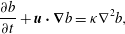 $$\begin{eqnarray}\displaystyle & \displaystyle \frac{\partial b}{\partial t}+\boldsymbol{u}\boldsymbol{\cdot }\boldsymbol{{\rm\nabla}}b={\it\kappa}{\rm\nabla}^{2}b, & \displaystyle\end{eqnarray}$$
where $\boldsymbol{u}\equiv (u,v,w)$
is the velocity, with components in the radial, azimuthal and longitudinal directions, respectively,
$\boldsymbol{u}\equiv (u,v,w)$
is the velocity, with components in the radial, azimuthal and longitudinal directions, respectively, $p$
is the kinematic pressure relative to a hydrostatic balance and
$p$
is the kinematic pressure relative to a hydrostatic balance and ${\it\nu}$
and
${\it\nu}$
and ${\it\kappa}$
are the kinematic viscosity and buoyancy diffusion coefficient, respectively. Noting the statistical axisymmetry of the flow, an ensemble and azimuthal average of (2.2)–(2.4) in the limit of high Reynolds and Péclet numbers yields
${\it\kappa}$
are the kinematic viscosity and buoyancy diffusion coefficient, respectively. Noting the statistical axisymmetry of the flow, an ensemble and azimuthal average of (2.2)–(2.4) in the limit of high Reynolds and Péclet numbers yields
 $$\begin{eqnarray}\displaystyle & \displaystyle \frac{1}{r}\frac{\partial (r\overline{u})}{\partial r}+\frac{\partial \overline{w}}{\partial z}=0, & \displaystyle\end{eqnarray}$$
 $$\begin{eqnarray}\displaystyle & \displaystyle \frac{\partial \overline{w}}{\partial t}+\frac{1}{r}\frac{\partial }{\partial r}(r\overline{u}\,\overline{w}+r\overline{u^{\prime }w^{\prime }})+\frac{\partial }{\partial z}(\overline{w}^{2}+\overline{w^{\prime 2}})=-\frac{\partial \overline{p}}{\partial z}+\overline{b}, & \displaystyle\end{eqnarray}$$
 $$\begin{eqnarray}\displaystyle & \displaystyle \frac{\partial \overline{b}}{\partial t}+\frac{1}{r}\frac{\partial }{\partial r}(r\overline{u}\,\overline{b}+r\overline{u^{\prime }b^{\prime }})+\frac{\partial }{\partial z}(\overline{w}\overline{b}+\overline{w^{\prime }b^{\prime }})=0. & \displaystyle\end{eqnarray}$$
Here $\overline{{\it\chi}}$
denotes the ensemble average of the variable
$\overline{{\it\chi}}$
denotes the ensemble average of the variable ${\it\chi}$
, so that
${\it\chi}$
, so that ${\it\chi}\equiv \overline{{\it\chi}}+{\it\chi}^{\prime }$
, where
${\it\chi}\equiv \overline{{\it\chi}}+{\it\chi}^{\prime }$
, where $\overline{{\it\chi}^{\prime }}=0$
. Multiplication of (2.6) by
$\overline{{\it\chi}^{\prime }}=0$
. Multiplication of (2.6) by $2\overline{w}$
yields an equation for the mean longitudinal kinetic energy:
$2\overline{w}$
yields an equation for the mean longitudinal kinetic energy:
 $$\begin{eqnarray}\displaystyle & & \displaystyle \frac{\partial \overline{w}^{2}}{\partial t}+\frac{1}{r}\frac{\partial (r\overline{u}\,\overline{w}^{2})}{\partial r}+\frac{\partial \overline{w}^{3}}{\partial z}+2\frac{\partial (\overline{p}\,\overline{w})}{\partial z}+\frac{2}{r}\frac{\partial (r\overline{u^{\prime }w^{\prime }}\overline{w})}{\partial r}+2\,\frac{\partial (\overline{w^{\prime 2}}\overline{w})}{\partial z}\nonumber\\ \displaystyle & & \displaystyle \quad =2\overline{p}\frac{\partial \overline{w}}{\partial z}+2\,\overline{w^{\prime 2}}\frac{\partial \overline{w}}{\partial z}+2\,\overline{u^{\prime }w^{\prime }}\frac{\partial \overline{w}}{\partial r}+2\overline{b}\overline{w}.\end{eqnarray}$$
Due to the fact that $\overline{w}\gg \overline{u},\overline{v}$
we will omit ‘longitudinal’ in describing (2.8) hereafter, referring to it instead as the equation for the mean kinetic energy. For further details pertaining to the derivation of (2.5)–(2.8) the reader is referred to Craske & van Reeuwijk (Reference Craske and van Reeuwijk2015a
).
$\overline{w}\gg \overline{u},\overline{v}$
we will omit ‘longitudinal’ in describing (2.8) hereafter, referring to it instead as the equation for the mean kinetic energy. For further details pertaining to the derivation of (2.5)–(2.8) the reader is referred to Craske & van Reeuwijk (Reference Craske and van Reeuwijk2015a
).
Having been obtained via invertible manipulations, the momentum–energy system (2.6) and (2.8), is equivalent to the volume–momentum system, (2.5) and (2.6). Both satisfy local volume and momentum conservation, but whereas (2.5) is a diagnostic relation or constraint, (2.8) is a prognostic equation. In the following section we will show that the momentum–energy system constitutes the natural choice for developing and understanding integral models of unsteady plumes.
2.2 Integral equations
Integration of (2.6)–(2.8) with respect to $r$
from zero to the radial extent of the plume
$r$
from zero to the radial extent of the plume $r_{d}$
, yields the integral equations
$r_{d}$
, yields the integral equations
 $$\begin{eqnarray}\displaystyle & \displaystyle \frac{\partial Q}{\partial t}+\frac{\partial ({\it\beta}_{g}M)}{\partial z}=B, & \displaystyle\end{eqnarray}$$
 $$\begin{eqnarray}\displaystyle & \displaystyle \frac{\partial M}{\partial t}+\frac{\partial }{\partial z}\left({\it\gamma}_{g}\frac{M^{2}}{Q}\right)={\it\delta}_{g}\frac{M^{5/2}}{Q^{2}}+2{\it\theta}_{m}\frac{MB}{Q}, & \displaystyle\end{eqnarray}$$
 $$\begin{eqnarray}\displaystyle & \displaystyle \frac{\partial B}{\partial t}+\frac{\partial }{\partial z}\left({\it\theta}_{g}\frac{MB}{Q}\right)=0, & \displaystyle\end{eqnarray}$$
where the dependent variables are the longitudinal volume flux $Q$
, the longitudinal specific momentum flux
$Q$
, the longitudinal specific momentum flux $M$
(hereafter referred to as the momentum flux for brevity) and the integral buoyancy
$M$
(hereafter referred to as the momentum flux for brevity) and the integral buoyancy $B$
:
$B$
:
 $$\begin{eqnarray}Q\equiv 2\int _{0}^{r_{d}}\overline{w}r\,\text{d}r,\quad M\equiv 2\int _{0}^{r_{d}}\overline{w}^{2}r\,\text{d}r,\quad B\equiv 2\int _{0}^{r_{d}}\overline{b}r\,\text{d}r.\end{eqnarray}$$
The Greek letters in (2.9)–(2.11) are dimensionless profile coefficients that allow us to express unknown integrals in terms of the dependent variables $Q$
,
$Q$
, $M$
and
$M$
and $B$
, and are defined as
$B$
, and are defined as
 $$\begin{eqnarray}\displaystyle & \displaystyle {\it\beta}_{g}\equiv \underbrace{\frac{2}{M}\int _{0}^{r_{d}}\overline{w}^{2}r\,\text{d}r}_{{\it\beta}_{m}}+\underbrace{\frac{2}{M}\int _{0}^{r_{d}}\overline{w^{\prime 2}}r\,\text{d}r}_{{\it\beta}_{f}}+\underbrace{\frac{2}{M}\int _{0}^{r_{d}}\overline{p}r\,\text{d}r}_{{\it\beta}_{p}}, & \displaystyle\end{eqnarray}$$
 $$\begin{eqnarray}\displaystyle & \displaystyle {\it\gamma}_{g}\equiv \underbrace{\frac{2Q}{M^{2}}\int _{0}^{r_{d}}r\overline{w}^{3}r\,\text{d}r}_{{\it\gamma}_{m}}+\underbrace{\frac{4Q}{M^{2}}\int _{0}^{r_{d}}r\overline{w}\overline{w^{\prime 2}}r\,\text{d}r}_{{\it\gamma}_{f}}+\underbrace{\frac{4Q}{M^{2}}\int _{0}^{r_{d}}\overline{p}\,\overline{w}r\,\text{d}r}_{{\it\gamma}_{p}}, & \displaystyle\end{eqnarray}$$
 $$\begin{eqnarray}\displaystyle & \displaystyle {\it\theta}_{g}\equiv \underbrace{\frac{2Q}{BM}\int _{0}^{r_{d}}\overline{w}\overline{b}r\,\text{d}r}_{{\it\theta}_{m}}+\underbrace{\frac{2Q}{BM}\int _{0}^{r_{d}}\overline{w^{\prime }b^{\prime }}r\,\text{d}r}_{{\it\theta}_{f}}, & \displaystyle\end{eqnarray}$$
 $$\begin{eqnarray}\displaystyle & \displaystyle {\it\delta}_{g}\equiv \underbrace{\frac{4Q^{2}}{M^{5/2}}\int _{0}^{r_{d}}\overline{u^{\prime }w^{\prime }}\frac{\partial \overline{w}}{\partial r}r\,\text{d}r}_{{\it\delta}_{m}}+\underbrace{\frac{4Q^{2}}{M^{5/2}}\int _{0}^{r_{d}}\overline{w^{\prime 2}}\frac{\partial \overline{w}}{\partial z}r\,\text{d}r}_{{\it\delta}_{f}}+\underbrace{\frac{4Q^{2}}{M^{5/2}}\int _{0}^{r_{d}}\overline{p}\,\frac{\partial \overline{w}}{\partial z}r\,\text{d}r}_{{\it\delta}_{p}}. & \displaystyle\end{eqnarray}$$
We refer to (2.9)–(2.11) as generalised unsteady plume equations, because we have not yet made an assumption about the way in which the dimensionless profile coefficients might depend on $z$
,
$z$
, $t$
,
$t$
, $Q$
,
$Q$
, $M$
or
$M$
or $B$
. Physically, the profile coefficients
$B$
. Physically, the profile coefficients ${\it\beta}_{g}$
,
${\it\beta}_{g}$
, ${\it\gamma}_{g}$
,
${\it\gamma}_{g}$
, ${\it\theta}_{g}$
and
${\it\theta}_{g}$
and ${\it\delta}_{g}$
correspond to gross dimensionless fluxes of momentum, energy and buoyancy, and the gross dimensionless production of turbulence kinetic energy (including the redistribution of energy via pressure), respectively. Note that
${\it\delta}_{g}$
correspond to gross dimensionless fluxes of momentum, energy and buoyancy, and the gross dimensionless production of turbulence kinetic energy (including the redistribution of energy via pressure), respectively. Note that ${\it\theta}_{g}$
is used in (2.11) because it accounts for the total transport of buoyancy, whereas
${\it\theta}_{g}$
is used in (2.11) because it accounts for the total transport of buoyancy, whereas ${\it\theta}_{m}$
is used in (2.10) because the forcing of the mean flow energy by buoyancy does not include turbulent transport
${\it\theta}_{m}$
is used in (2.10) because the forcing of the mean flow energy by buoyancy does not include turbulent transport ${\it\theta}_{f}$
. In addition, note that
${\it\theta}_{f}$
. In addition, note that ${\it\beta}_{m}$
in (2.13), which we include for completeness, is unity by definition. In obtaining (2.9)–(2.11) it was assumed that the ensemble and azimuthally averaged velocity
${\it\beta}_{m}$
in (2.13), which we include for completeness, is unity by definition. In obtaining (2.9)–(2.11) it was assumed that the ensemble and azimuthally averaged velocity $\overline{w}$
and buoyancy
$\overline{w}$
and buoyancy $\overline{b}$
are equal to zero at
$\overline{b}$
are equal to zero at $r=r_{d}$
.
$r=r_{d}$
.
Before proceeding, we note that the integral buoyancy $B$
is not used in steady plume theory, in which the effects of buoyancy are typically expressed in terms of the mean buoyancy flux
$B$
is not used in steady plume theory, in which the effects of buoyancy are typically expressed in terms of the mean buoyancy flux $F\equiv {\it\theta}_{m}MB/Q$
(see, e.g. Hunt & van den Bremer Reference Hunt and van den Bremer2011, and references therein):
$F\equiv {\it\theta}_{m}MB/Q$
(see, e.g. Hunt & van den Bremer Reference Hunt and van den Bremer2011, and references therein):
 $$\begin{eqnarray}F\equiv 2\int _{0}^{r_{d}}\overline{w}\,\overline{b}r\,\text{d}r.\end{eqnarray}$$
However, in the unsteady integral equations (2.9)–(2.11), the use of $B$
is convenient from both a mathematical and a conceptual perspective. With
$B$
is convenient from both a mathematical and a conceptual perspective. With $B$
as a dependent variable, the temporal derivatives in (2.9)–(2.11) are decoupled and each obeys a classical conservation equation. Moreover, it is natural to view the buoyancy flux
$B$
as a dependent variable, the temporal derivatives in (2.9)–(2.11) are decoupled and each obeys a classical conservation equation. Moreover, it is natural to view the buoyancy flux $F$
as an unknown quantity requiring assumptions because it depends on the correlation of
$F$
as an unknown quantity requiring assumptions because it depends on the correlation of $\overline{w}$
and
$\overline{w}$
and $\overline{b}$
. In this regard, we also note that while we do not advocate using the continuity equation (2.5) directly, the behaviour of the volume flux
$\overline{b}$
. In this regard, we also note that while we do not advocate using the continuity equation (2.5) directly, the behaviour of the volume flux $Q$
nevertheless plays a crucial role in the system (2.9)–(2.11) as a dependent variable.
$Q$
nevertheless plays a crucial role in the system (2.9)–(2.11) as a dependent variable.
2.3 Modelling assumptions
The central message of this paper is that each of the dimensionless profile coefficients appearing in (2.9)–(2.11) play an independent and non-trivial role in determining the structure of the governing equations. In a steady state, for which $\partial _{t}=0$
, the situation is different because the profile coefficients no longer play an independent role. Therefore, the form of the classical steady-state power-law solutions, which will be discussed in § 2.5, are essentially independent of the values of the profile coefficients. In a steady state the influence that the profile coefficients have on the behaviour of the system is hidden.
$\partial _{t}=0$
, the situation is different because the profile coefficients no longer play an independent role. Therefore, the form of the classical steady-state power-law solutions, which will be discussed in § 2.5, are essentially independent of the values of the profile coefficients. In a steady state the influence that the profile coefficients have on the behaviour of the system is hidden.
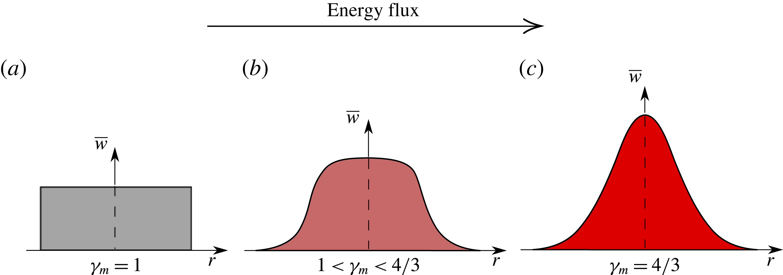
Figure 1. The mean dimensionless energy flux ${\it\gamma}_{m}$
associated with different radial profiles of the longitudinal velocity. The top-hat profile (a) is a limiting case for which the dimensionless energy flux is minimal, while in the case of a Gaussian profile (c)
${\it\gamma}_{m}$
associated with different radial profiles of the longitudinal velocity. The top-hat profile (a) is a limiting case for which the dimensionless energy flux is minimal, while in the case of a Gaussian profile (c) ${\it\gamma}_{m}=4/3$
.
${\it\gamma}_{m}=4/3$
.
By definition, the assumed shape of the mean velocity profile does not affect the volume flux or the momentum flux in the plume, i.e. the volume flux and the momentum flux are equal to $Q$
and
$Q$
and $M$
, respectively, regardless of the behaviour of
$M$
, respectively, regardless of the behaviour of $\overline{w}$
. Similarly the shape of the buoyancy profile does not, by definition, affect the integral buoyancy
$\overline{w}$
. Similarly the shape of the buoyancy profile does not, by definition, affect the integral buoyancy $B$
. In self-similar steady-state models of jets and plumes it is therefore conventional (Turner Reference Turner1973), and entails no loss of generality, to regard
$B$
. In self-similar steady-state models of jets and plumes it is therefore conventional (Turner Reference Turner1973), and entails no loss of generality, to regard $\overline{w}$
as having a uniform distribution of amplitude
$\overline{w}$
as having a uniform distribution of amplitude $w_{m}$
for
$w_{m}$
for $r\leqslant r_{m}$
, which is known as a top-hat distribution, as illustrated in figure 1(a). However, the assumed velocity profile does affect the mean energy flux
$r\leqslant r_{m}$
, which is known as a top-hat distribution, as illustrated in figure 1(a). However, the assumed velocity profile does affect the mean energy flux ${\it\gamma}_{m}M^{2}/Q$
in the plume, because
${\it\gamma}_{m}M^{2}/Q$
in the plume, because ${\it\gamma}_{m}$
depends on the radial dependence of the velocity field. In unsteady jets and plumes, unlike their statistically steady counterparts, the energy flux plays an independent role in the governing equations and therefore, the assumption of a particular velocity profile does entail a loss of generality. A useful result in this regard is that for a Gaussian mean velocity profile
${\it\gamma}_{m}$
depends on the radial dependence of the velocity field. In unsteady jets and plumes, unlike their statistically steady counterparts, the energy flux plays an independent role in the governing equations and therefore, the assumption of a particular velocity profile does entail a loss of generality. A useful result in this regard is that for a Gaussian mean velocity profile $\overline{w}(r)$
, illustrated in figure 1(c), the dimensionless energy flux
$\overline{w}(r)$
, illustrated in figure 1(c), the dimensionless energy flux ${\it\gamma}_{m}$
can be determined exactly (Craske & van Reeuwijk Reference Craske and van Reeuwijk2015a
) as
${\it\gamma}_{m}$
can be determined exactly (Craske & van Reeuwijk Reference Craske and van Reeuwijk2015a
) as
 $$\begin{eqnarray}{\it\gamma}_{m}=\frac{16}{r_{m}^{2}}\lim _{r_{d}\rightarrow \infty }\int _{0}^{r_{d}}\exp \left(-6\frac{r^{2}}{r_{m}^{2}}\right)r\,\text{d}r=\frac{4}{3}.\end{eqnarray}$$
The mean energy flux associated with top-hat velocity profiles, on the other hand, is minimal (assuming that $\overline{w}>0$
), such that
$\overline{w}>0$
), such that ${\it\gamma}_{m}=1$
. It is evident from (2.14) that any variation in the radial dependence of the velocity profile will result in
${\it\gamma}_{m}=1$
. It is evident from (2.14) that any variation in the radial dependence of the velocity profile will result in ${\it\gamma}_{m}>1$
, as illustrated schematically in figure 1. Although Hewitt & Bonnebaigt (Reference Hewitt and Bonnebaigt2014) remark that integral models of turbulent plumes remove information pertaining to radial dependence, we find that this is not necessarily the case. Use of the mean kinetic energy equation exposes the fact that
${\it\gamma}_{m}>1$
, as illustrated schematically in figure 1. Although Hewitt & Bonnebaigt (Reference Hewitt and Bonnebaigt2014) remark that integral models of turbulent plumes remove information pertaining to radial dependence, we find that this is not necessarily the case. Use of the mean kinetic energy equation exposes the fact that ${\it\gamma}_{m}$
appears as an independent parameter, determining the response of the plume to source perturbations and the trajectories of its characteristic curves.
${\it\gamma}_{m}$
appears as an independent parameter, determining the response of the plume to source perturbations and the trajectories of its characteristic curves.
2.4 Volume conservation
The motivation for working with the mean kinetic energy equation (2.8) rather than the continuity equation (2.2) is that the radial integral of (2.2),
 $$\begin{eqnarray}\frac{\partial Q}{\partial z}=-2ru|_{\infty },\end{eqnarray}$$
does not provide an explicit prognostic equation (for definiteness and consistency with the classical approach, here we have assumed that $r_{d}\rightarrow \infty$
in (2.12)). Instead, (2.19), which is ostensibly identical to the steady-state volume flux equation given by Morton et al. (Reference Morton, Taylor and Turner1956), relates the volume flux in the plume to the induced radial velocity in the environment. Indeed, (2.19) can be used in place of the integral energy equation (2.10), but the modeller is then faced with the task of providing a closure for
$r_{d}\rightarrow \infty$
in (2.12)). Instead, (2.19), which is ostensibly identical to the steady-state volume flux equation given by Morton et al. (Reference Morton, Taylor and Turner1956), relates the volume flux in the plume to the induced radial velocity in the environment. Indeed, (2.19) can be used in place of the integral energy equation (2.10), but the modeller is then faced with the task of providing a closure for $ru|_{\infty }$
. In the steady state, Morton et al. (Reference Morton, Taylor and Turner1956) replace the right-hand side of (2.19) with
$ru|_{\infty }$
. In the steady state, Morton et al. (Reference Morton, Taylor and Turner1956) replace the right-hand side of (2.19) with $2{\it\alpha}_{0}M^{1/2}$
, thereby defining the classical entrainment coefficient
$2{\it\alpha}_{0}M^{1/2}$
, thereby defining the classical entrainment coefficient ${\it\alpha}_{0}$
, to obtain a closed system of equations. In the unsteady case, however, an induced radial flow in the environment does not necessarily correspond to entrainment into the plume, because the radius of the plume might change with respect to time (cf. the temporal jet studied by van Reeuwijk & Holzner Reference van Reeuwijk and Holzner2014, for example). Conversely, efforts to obtain a prognostic equation for the area
${\it\alpha}_{0}$
, to obtain a closed system of equations. In the unsteady case, however, an induced radial flow in the environment does not necessarily correspond to entrainment into the plume, because the radius of the plume might change with respect to time (cf. the temporal jet studied by van Reeuwijk & Holzner Reference van Reeuwijk and Holzner2014, for example). Conversely, efforts to obtain a prognostic equation for the area $r_{m}^{2}\equiv Q^{2}/M$
of the plume rely on particular assumptions regarding its velocity profile. In all but the simplest cases (e.g. the rigorously derived top-hat model of Scase et al. (Reference Scase, Caulfield, Dalziel and Hunt2006b
)), such models have questionable foundations, because typically, ensemble-averaged quantities in plumes do not have a well-defined edge and depend continuously on the radial coordinate. The use of a generalised plume theory, resulting in (2.9)–(2.11), circumvents these issues altogether and allows one to understand unsteady plume models in a broader context. Consequently, the theory provides a physics-based means of understanding and remedying the problems associated with existing unsteady plume models (for details of these problems see Scase & Hewitt (Reference Scase and Hewitt2012)).
$r_{m}^{2}\equiv Q^{2}/M$
of the plume rely on particular assumptions regarding its velocity profile. In all but the simplest cases (e.g. the rigorously derived top-hat model of Scase et al. (Reference Scase, Caulfield, Dalziel and Hunt2006b
)), such models have questionable foundations, because typically, ensemble-averaged quantities in plumes do not have a well-defined edge and depend continuously on the radial coordinate. The use of a generalised plume theory, resulting in (2.9)–(2.11), circumvents these issues altogether and allows one to understand unsteady plume models in a broader context. Consequently, the theory provides a physics-based means of understanding and remedying the problems associated with existing unsteady plume models (for details of these problems see Scase & Hewitt (Reference Scase and Hewitt2012)).
From the integral equations for momentum (2.9) and mean energy (2.10), one can obtain a prognostic equation for the area of the plume without assumption. To appreciate this, note that the continuity equation (2.2) was used to obtain the mean energy equation (2.8) from the mean momentum equation (2.6). Together, (2.6) and (2.8) therefore imply the continuity equation (2.2). Similarly, one can recover an integral volume conservation equation by combining integral equations for momentum (2.9) and mean energy (2.10). A consistent equation for the area of the plume is therefore obtained by expanding $\partial _{t}(Q^{2}/M)$
and substituting for
$\partial _{t}(Q^{2}/M)$
and substituting for $\partial _{t}Q$
and
$\partial _{t}Q$
and $\partial _{t}M$
using (2.9) and (2.10) respectively:
$\partial _{t}M$
using (2.9) and (2.10) respectively:
 $$\begin{eqnarray}\frac{1}{{\it\gamma}_{g}}\frac{\partial }{\partial t}\left(\frac{Q^{2}}{M}\right)+\frac{\partial Q}{\partial z}=2{\it\alpha}M^{1/2},\end{eqnarray}$$
where
 $$\begin{eqnarray}\displaystyle {\it\alpha}\equiv -\frac{{\it\delta}_{g}}{2{\it\gamma}_{g}}+\frac{Q}{2{\it\gamma}_{g}M^{5/2}}\frac{\partial }{\partial z}[({\it\gamma}_{g}-2{\it\beta}_{g}+1)M^{2}]+\frac{Q}{{\it\gamma}_{g}M^{3/2}}({\it\beta}_{g}-1)\frac{\partial M}{\partial z}+\left(\frac{1}{{\it\gamma}_{g}}-\frac{{\it\theta}_{m}}{{\it\gamma}_{g}}\right)\frac{QB}{M^{3/2}}.\hspace{-9.60004pt} & & \displaystyle \nonumber\\ \displaystyle & & \displaystyle\end{eqnarray}$$
The advantage of (2.20) and (2.21) in comparison with (2.19) is that not only do they account explicitly for the temporal change of the area of the jet, they account for the process of entrainment in terms of known physical processes such as the production of turbulence kinetic energy and the transport of mean kinetic energy. As described in van Reeuwijk & Craske (Reference van Reeuwijk and Craske2015), (2.21) is an entrainment relation that ensures consistency between equations for volume, momentum and energy conservation. Equation (2.21) is not an entrainment model because we have not assigned values/functions to the profile coefficients ${\it\beta}_{g}$
,
${\it\beta}_{g}$
, ${\it\gamma}_{g}$
,
${\it\gamma}_{g}$
, ${\it\theta}_{g}$
and
${\it\theta}_{g}$
and ${\it\delta}_{g}$
by invoking assumptions.
${\it\delta}_{g}$
by invoking assumptions.
There are two significant features of (2.20). First is the factor $1/{\it\gamma}_{g}$
preceding
$1/{\it\gamma}_{g}$
preceding $\partial _{t}(Q^{2}/M)$
, which, by implying an effective area
$\partial _{t}(Q^{2}/M)$
, which, by implying an effective area $Q^{2}/(M{\it\gamma}_{g})$
, provides a definition of the plume edge for continuous velocity profiles. Reassuringly, for top-hat profiles
$Q^{2}/(M{\it\gamma}_{g})$
, provides a definition of the plume edge for continuous velocity profiles. Reassuringly, for top-hat profiles ${\it\gamma}_{g}=1$
, which makes the left-hand side of (2.20) consistent with the top-hat model of Scase et al. (Reference Scase, Caulfield, Dalziel and Hunt2006b
). Second, is the entrainment coefficient
${\it\gamma}_{g}=1$
, which makes the left-hand side of (2.20) consistent with the top-hat model of Scase et al. (Reference Scase, Caulfield, Dalziel and Hunt2006b
). Second, is the entrainment coefficient ${\it\alpha}$
, which is not necessarily constant. The first contribution on the right-hand side of (2.21) accounts for the production of turbulence kinetic energy and typically dominates the remaining terms. When the profile coefficients are constant, it is useful to regard the second and third terms on the right-hand side of (2.21) as relating to the integral advective acceleration of the plume
${\it\alpha}$
, which is not necessarily constant. The first contribution on the right-hand side of (2.21) accounts for the production of turbulence kinetic energy and typically dominates the remaining terms. When the profile coefficients are constant, it is useful to regard the second and third terms on the right-hand side of (2.21) as relating to the integral advective acceleration of the plume $\partial _{z}M$
. Note, however, that due to entrainment
$\partial _{z}M$
. Note, however, that due to entrainment $\partial _{z}M>0$
does not always imply a local advective acceleration
$\partial _{z}M>0$
does not always imply a local advective acceleration $\partial _{z}w_{m}>0$
, but nevertheless accounts for the way in which the plume is forced in an integral sense. How entrainment is affected by the plume’s integral acceleration depends on the radial dependence of the velocity, turbulence and pressure. For top-hat profiles
$\partial _{z}w_{m}>0$
, but nevertheless accounts for the way in which the plume is forced in an integral sense. How entrainment is affected by the plume’s integral acceleration depends on the radial dependence of the velocity, turbulence and pressure. For top-hat profiles ${\it\gamma}_{g}={\it\beta}_{g}=1$
, the entrainment coefficient is insensitive to the integral acceleration of the plume and the second and third terms on the right-hand side of (2.21) are equal to zero. For further details regarding the physical interpretation of the first three terms on the right-hand side of (2.21), the reader is referred to Craske & van Reeuwijk (Reference Craske and van Reeuwijk2015a
), as they also appear in the equations describing an unsteady jet. The final contribution in (2.21) is only found in plumes and is proportional to the flux-balance parameter
${\it\gamma}_{g}={\it\beta}_{g}=1$
, the entrainment coefficient is insensitive to the integral acceleration of the plume and the second and third terms on the right-hand side of (2.21) are equal to zero. For further details regarding the physical interpretation of the first three terms on the right-hand side of (2.21), the reader is referred to Craske & van Reeuwijk (Reference Craske and van Reeuwijk2015a
), as they also appear in the equations describing an unsteady jet. The final contribution in (2.21) is only found in plumes and is proportional to the flux-balance parameter ${\it\Gamma}$
of Morton (Reference Morton1959). If
${\it\Gamma}$
of Morton (Reference Morton1959). If ${\it\theta}_{m}>1$
, the buoyancy provides slightly more forcing in the energy equation (2.10) than one would expect from identically distributed
${\it\theta}_{m}>1$
, the buoyancy provides slightly more forcing in the energy equation (2.10) than one would expect from identically distributed $\overline{b}$
and
$\overline{b}$
and $\overline{w}$
. Noting that the area
$\overline{w}$
. Noting that the area $Q^{2}/M$
is inversely proportional to the momentum flux
$Q^{2}/M$
is inversely proportional to the momentum flux $M$
, the effect of
$M$
, the effect of ${\it\theta}_{m}>1$
is to reduce the entrainment coefficient. Conversely, when
${\it\theta}_{m}>1$
is to reduce the entrainment coefficient. Conversely, when ${\it\theta}_{m}<1$
the buoyancy provides slightly less forcing in the energy equation than one might expect, and the entrainment coefficient increases.
${\it\theta}_{m}<1$
the buoyancy provides slightly less forcing in the energy equation than one might expect, and the entrainment coefficient increases.
In appendix A we derive generalised time-dependent similarity solutions of (2.9)–(2.11) involving an algebraic decrease in the plume’s source buoyancy flux. The solutions show that for Gaussian plumes the entrainment coefficient increases, relative to its steady-state value ${\it\alpha}_{0}$
, in such a way that the plume’s radius retains its steady-state dependence on
${\it\alpha}_{0}$
, in such a way that the plume’s radius retains its steady-state dependence on $z$
and is independent of time. Conversely, in plumes with a top-hat velocity profile, the solutions predict that the entrainment coefficient is always equal to
$z$
and is independent of time. Conversely, in plumes with a top-hat velocity profile, the solutions predict that the entrainment coefficient is always equal to ${\it\alpha}_{0}$
and that the spreading rate of the plume decreases relative to that associated with the steady state due to the time dependence of the source conditions, the latter result being first obtained by Scase et al. (Reference Scase, Caulfield, Dalziel and Hunt2006b
).
${\it\alpha}_{0}$
and that the spreading rate of the plume decreases relative to that associated with the steady state due to the time dependence of the source conditions, the latter result being first obtained by Scase et al. (Reference Scase, Caulfield, Dalziel and Hunt2006b
).
2.5 The steady state
Using the momentum–energy formulation (2.9)–(2.11), it is interesting to see how the profile coefficients can be incorporated into the classical steady-state plume solutions. For constant source buoyancy flux $F_{s}$
and constant profile coefficients, the latter assumption being consistent with far-field self-similarity, a steady-state solution to (2.9)–(2.11), which we denote
$F_{s}$
and constant profile coefficients, the latter assumption being consistent with far-field self-similarity, a steady-state solution to (2.9)–(2.11), which we denote $(Q_{0},M_{0},B_{0})$
, is
$(Q_{0},M_{0},B_{0})$
, is
 $$\begin{eqnarray}\left.\begin{array}{@{}c@{}}\displaystyle Q=Q_{0}(z)\equiv \frac{6{\it\alpha}_{0}}{5}\left(\frac{9{\it\alpha}_{0}}{10}\right)^{1/3}\left(\frac{F_{s}}{{\it\beta}_{g}{\it\theta}_{g}}\right)^{1/3}z^{5/3},\\ \displaystyle M=M_{0}(z)\equiv \left(\frac{9{\it\alpha}_{0}}{10}\right)^{2/3}\left(\frac{F_{s}}{{\it\beta}_{g}{\it\theta}_{g}}\right)^{2/3}z^{4/3},\end{array}\right\}\end{eqnarray}$$
where the constant steady-state entrainment coefficient, which follows from substitution of (2.22) into (2.10), is
 $$\begin{eqnarray}{\it\alpha}_{0}\equiv -\frac{{\it\delta}_{g}}{2{\it\gamma}_{g}}\left(\frac{8{\it\beta}_{g}{\it\theta}_{m}}{5{\it\gamma}_{g}}-\frac{3}{5}\right)^{-1}.\end{eqnarray}$$
Noting that the steady-state mean buoyancy flux $F$
is related to
$F$
is related to $F_{s}$
according to
$F_{s}$
according to $F={\it\theta}_{m}F_{s}/{\it\theta}_{g}$
, and that
$F={\it\theta}_{m}F_{s}/{\it\theta}_{g}$
, and that $B=FQ/({\it\theta}_{m}M)$
, the solution to the steady-state integral buoyancy
$B=FQ/({\it\theta}_{m}M)$
, the solution to the steady-state integral buoyancy $B_{0}$
is
$B_{0}$
is
 $$\begin{eqnarray}B=B_{0}(z)\equiv \frac{6{\it\alpha}_{0}}{5}\left(\frac{10}{9{\it\alpha}_{0}}\right)^{1/3}\left(\frac{F_{s}^{2}{\it\beta}_{g}}{{\it\theta}_{g}^{2}}\right)^{1/3}z^{1/3}.\end{eqnarray}$$
The effects of ${\it\theta}_{g}$
and
${\it\theta}_{g}$
and ${\it\beta}_{g}$
are felt only via
${\it\beta}_{g}$
are felt only via ${\it\alpha}_{0}$
and an effective buoyancy flux
${\it\alpha}_{0}$
and an effective buoyancy flux $F_{E}\equiv F_{s}/({\it\beta}_{g}{\it\theta}_{g})$
(van Reeuwijk & Craske Reference van Reeuwijk and Craske2015), and do not affect the classical power-law scaling of the steady-state solutions. Due to the fact that
$F_{E}\equiv F_{s}/({\it\beta}_{g}{\it\theta}_{g})$
(van Reeuwijk & Craske Reference van Reeuwijk and Craske2015), and do not affect the classical power-law scaling of the steady-state solutions. Due to the fact that $F_{s}={\it\theta}_{g}F/{\it\theta}_{m}$
, (2.22) can also be expressed in terms of the mean buoyancy flux
$F_{s}={\it\theta}_{g}F/{\it\theta}_{m}$
, (2.22) can also be expressed in terms of the mean buoyancy flux $F$
. Noting that the use of the total source buoyancy flux
$F$
. Noting that the use of the total source buoyancy flux $F_{s}$
, rather than the effective source buoyancy flux
$F_{s}$
, rather than the effective source buoyancy flux $F_{E}$
, would lead to an over-estimation of
$F_{E}$
, would lead to an over-estimation of $Q$
and
$Q$
and $M$
, the solutions (2.22) might be useful to experimentalists who wish to compare data to theory using a known source buoyancy flux
$M$
, the solutions (2.22) might be useful to experimentalists who wish to compare data to theory using a known source buoyancy flux $F_{s}$
. Comparison of the system (2.22) to the classical plume solutions of Morton et al. (Reference Morton, Taylor and Turner1956) shows that the flux-balance parameter of Morton (Reference Morton1959) is
$F_{s}$
. Comparison of the system (2.22) to the classical plume solutions of Morton et al. (Reference Morton, Taylor and Turner1956) shows that the flux-balance parameter of Morton (Reference Morton1959) is
 $$\begin{eqnarray}{\it\Gamma}\equiv \frac{5QB}{8{\it\beta}_{g}{\it\alpha}_{0}M^{3/2}}=\frac{5Q^{2}F}{8{\it\theta}_{m}{\it\beta}_{g}{\it\alpha}_{0}M^{5/2}},\end{eqnarray}$$
which characterises the relative importance of buoyancy compared with inertia in the flow. When $0<{\it\Gamma}<1$
, the plume is dominated by inertia and referred to as being ‘forced’; when
$0<{\it\Gamma}<1$
, the plume is dominated by inertia and referred to as being ‘forced’; when $1<{\it\Gamma}$
the plume is dominated by buoyancy and is referred to as being ‘lazy’. Jets and pure plumes correspond to the special cases for which
$1<{\it\Gamma}$
the plume is dominated by buoyancy and is referred to as being ‘lazy’. Jets and pure plumes correspond to the special cases for which ${\it\Gamma}=0$
or
${\it\Gamma}=0$
or ${\it\Gamma}=1$
, respectively. Thus, for the far-field similarity solutions (2.22), describing a pure plume, the fluxes of volume, momentum and buoyancy are balanced such that
${\it\Gamma}=1$
, respectively. Thus, for the far-field similarity solutions (2.22), describing a pure plume, the fluxes of volume, momentum and buoyancy are balanced such that ${\it\Gamma}=1$
. In general
${\it\Gamma}=1$
. In general ${\it\theta}_{m}\approx 1$
and
${\it\theta}_{m}\approx 1$
and ${\it\beta}_{g}>1$
, hence one would expect the classical definition of
${\it\beta}_{g}>1$
, hence one would expect the classical definition of ${\it\Gamma}$
, namely
${\it\Gamma}$
, namely $(5Q^{2}F)/(8{\it\alpha}_{0}M^{5/2})$
, to be slightly greater than unity, based on observations of
$(5Q^{2}F)/(8{\it\alpha}_{0}M^{5/2})$
, to be slightly greater than unity, based on observations of $Q$
,
$Q$
, $M$
and
$M$
and $F$
from a pure plume.
$F$
from a pure plume.
3 Simulation description
Data from the DNS of the Navier–Stokes equations were obtained using a domain of size $32\times 32\times 48$
source radii
$32\times 32\times 48$
source radii $r_{s}$
, uniformly discretised using
$r_{s}$
, uniformly discretised using $1024\times 1024\times 1536$
computational control volumes. For a detailed description of the finite volume method used to discretise the governing equations, the reader is referred to Craske & van Reeuwijk (Reference Craske and van Reeuwijk2015a
). On the vertical faces of the domain we use open boundary conditions that allow fluid to enter and leave the finite computational domain in a manner that is consistent with a semi-infinite unbounded domain. The formulation, testing and implementation of these boundary conditions is described in Craske & van Reeuwijk (Reference Craske and van Reeuwijk2013). The plumes we simulate are driven by an isolated circular source, of buoyancy flux
$1024\times 1024\times 1536$
computational control volumes. For a detailed description of the finite volume method used to discretise the governing equations, the reader is referred to Craske & van Reeuwijk (Reference Craske and van Reeuwijk2015a
). On the vertical faces of the domain we use open boundary conditions that allow fluid to enter and leave the finite computational domain in a manner that is consistent with a semi-infinite unbounded domain. The formulation, testing and implementation of these boundary conditions is described in Craske & van Reeuwijk (Reference Craske and van Reeuwijk2013). The plumes we simulate are driven by an isolated circular source, of buoyancy flux $F_{s}$
, located at the centre of the base of the domain at
$F_{s}$
, located at the centre of the base of the domain at $z=0$
. Fluxes of volume and momentum at the source are equal to zero; hence the plumes are lazy in the near field, with
$z=0$
. Fluxes of volume and momentum at the source are equal to zero; hence the plumes are lazy in the near field, with ${\it\Gamma}(z)\rightarrow \infty$
as
${\it\Gamma}(z)\rightarrow \infty$
as $z\rightarrow 0$
. The Prandtl number
$z\rightarrow 0$
. The Prandtl number $Pr\equiv {\it\nu}/{\it\kappa}$
(see (2.3) and (2.4)) used in the simulations is equal to 0.7, which corresponds to air. To initiate the turbulence we apply uncorrelated perturbations of amplitude 1 % to the velocities in the first cell above the source.
$Pr\equiv {\it\nu}/{\it\kappa}$
(see (2.3) and (2.4)) used in the simulations is equal to 0.7, which corresponds to air. To initiate the turbulence we apply uncorrelated perturbations of amplitude 1 % to the velocities in the first cell above the source.
Our ultimate aim was to obtain simulations of a plume whose source buoyancy flux undergoes a step change from $F_{s}^{B}$
to
$F_{s}^{B}$
to $F_{s}^{A}$
, where
$F_{s}^{A}$
, where $F_{s}^{B}<F_{s}^{A}$
. Therefore, we began by running two simulations L and H of steady-state plumes, with source buoyancy fluxes of
$F_{s}^{B}<F_{s}^{A}$
. Therefore, we began by running two simulations L and H of steady-state plumes, with source buoyancy fluxes of $F_{s}^{B}$
and
$F_{s}^{B}$
and $F_{s}^{A}$
, respectively, in order to validate the results and, in the case of L, to provide a set of initial conditions for the unsteady simulations. The Reynolds number
$F_{s}^{A}$
, respectively, in order to validate the results and, in the case of L, to provide a set of initial conditions for the unsteady simulations. The Reynolds number $\mathit{Re}_{s}\equiv 2F_{s}^{1/3}r_{s}^{2/3}/{\it\nu}$
was equal to 1320 and 1670 in L and H, respectively. The steady-state simulation L was run for a duration of approximately
$\mathit{Re}_{s}\equiv 2F_{s}^{1/3}r_{s}^{2/3}/{\it\nu}$
was equal to 1320 and 1670 in L and H, respectively. The steady-state simulation L was run for a duration of approximately $380{\it\tau}_{s}$
, where
$380{\it\tau}_{s}$
, where ${\it\tau}_{s}$
is the source turnover time,
${\it\tau}_{s}$
is the source turnover time, ${\it\tau}_{s}\equiv r_{s}^{4/3}F_{s}^{-1/3}$
. During simulation L we saved complete three-dimensional information of the flow field to disk at time intervals much larger than the turnover time. This information provided independent initial conditions for each unsteady simulation.
${\it\tau}_{s}\equiv r_{s}^{4/3}F_{s}^{-1/3}$
. During simulation L we saved complete three-dimensional information of the flow field to disk at time intervals much larger than the turnover time. This information provided independent initial conditions for each unsteady simulation.
Table 1. Simulation details. Here $F_{s}^{B}$
and
$F_{s}^{B}$
and $F_{s}^{A}$
denote the source buoyancy fluxes before and after the step change, respectively, and
$F_{s}^{A}$
denote the source buoyancy fluxes before and after the step change, respectively, and $\mathit{Re}_{s}\equiv 2F_{s}^{1/3}r_{s}^{2/3}/{\it\nu}$
is the source Reynolds number. The symbols L and H refer to simulations at a source Reynolds number of 1320 and 1670, corresponding to
$\mathit{Re}_{s}\equiv 2F_{s}^{1/3}r_{s}^{2/3}/{\it\nu}$
is the source Reynolds number. The symbols L and H refer to simulations at a source Reynolds number of 1320 and 1670, corresponding to $F_{s}^{B}$
and
$F_{s}^{B}$
and $F_{s}^{A}$
, respectively.
$F_{s}^{A}$
, respectively.

Using the three-dimensional field data obtained from L, unsteady plumes were created by imposing a step change in the source buoyancy flux from $F_{s}^{B}$
to
$F_{s}^{B}$
to $F_{s}^{A}$
. With the 24 statistically independent initial conditions, we repeated the process to obtain an ensemble of 24 unsteady plumes. The unsteady plume data was subsequently averaged over the ensemble and over the statistically homogeneous azimuthal dimension of the flow. To compute integrals over the radius of the plume we defined the upper limit of integration
$F_{s}^{A}$
. With the 24 statistically independent initial conditions, we repeated the process to obtain an ensemble of 24 unsteady plumes. The unsteady plume data was subsequently averaged over the ensemble and over the statistically homogeneous azimuthal dimension of the flow. To compute integrals over the radius of the plume we defined the upper limit of integration $r_{d}$
(see (2.12), for example) such that
$r_{d}$
(see (2.12), for example) such that $\overline{w}(r_{d},z,t)=\overline{w}(0,z,t)/100$
, which ensures that the longitudinal ambient velocity is small relative to that of the plume. Details of the simulations are summarised in table 1, and validation of the steady-state data is provided in appendix B.
$\overline{w}(r_{d},z,t)=\overline{w}(0,z,t)/100$
, which ensures that the longitudinal ambient velocity is small relative to that of the plume. Details of the simulations are summarised in table 1, and validation of the steady-state data is provided in appendix B.
4 Simulation results
4.1 Steady plumes
Before discussing the simulations of unsteady plumes we discuss those of steady plumes, focusing on the values of the dimensionless profile coefficients that were introduced in § 2. The profile coefficients, defined by (2.13)–(2.16), determine the relative importance of each term in the governing integral equations (2.9)–(2.11). Physically, they can be viewed as dimensionless flux and turbulence production/redistribution terms. As explained in §§ 2.3 and 2.5, while the profile coefficients play a passive role in a steady state, we will demonstrate in § 5 that in an unsteady state they play an active role in determining the structure of the governing equations. In order to make predictions about unsteady plumes, it is therefore useful to establish the values of the profile coefficients to leading order by inspecting the steady-state plume data. Whether the profile coefficients are themselves affected by unsteadiness is a higher-order question that we defer until § 6.1.
Table 2. The dimensionless parameters of a steady plume. Here TH $=$
top-hat, G
$=$
top-hat, G $=$
Gaussian and H and L refer to direct numerical simulation at a Reynolds number of 1670 and 1320, respectively (see § 3 for further details). The entrainment coefficient in a plume is denoted
$=$
Gaussian and H and L refer to direct numerical simulation at a Reynolds number of 1670 and 1320, respectively (see § 3 for further details). The entrainment coefficient in a plume is denoted ${\it\alpha}$
(
${\it\alpha}$
( ${\it\alpha}_{0}$
denoting the value of
${\it\alpha}_{0}$
denoting the value of ${\it\alpha}$
in a steady state) and is discussed at length in § 2.4. For the definitions of the remaining dimensionless profile coefficients (Greek letters), the reader is referred to § 2.2.
${\it\alpha}$
in a steady state) and is discussed at length in § 2.4. For the definitions of the remaining dimensionless profile coefficients (Greek letters), the reader is referred to § 2.2.
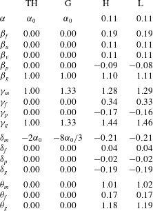
Table 2 displays the values of the profile coefficients evaluated from the steady-state data provided by simulations L and H. The values were obtained by averaging over the interval $z/r_{s}\in [20,40]$
, in which the profile coefficients were observed to have reached an approximately constant value. The near field, in which the profile coefficients exhibit appreciable variation, is not investigated in this work. To begin, it is useful to recall that
$z/r_{s}\in [20,40]$
, in which the profile coefficients were observed to have reached an approximately constant value. The near field, in which the profile coefficients exhibit appreciable variation, is not investigated in this work. To begin, it is useful to recall that ${\it\beta}_{m}$
,
${\it\beta}_{m}$
, ${\it\gamma}_{m}$
and
${\it\gamma}_{m}$
and ${\it\theta}_{m}$
are the leading-order dimensionless mean fluxes of momentum, energy and buoyancy. The dimensionless production
${\it\theta}_{m}$
are the leading-order dimensionless mean fluxes of momentum, energy and buoyancy. The dimensionless production ${\it\delta}_{m}$
is also of leading order but, due to the difference between the longitudinal and radial length scale of the plume, is smaller than
${\it\delta}_{m}$
is also of leading order but, due to the difference between the longitudinal and radial length scale of the plume, is smaller than ${\it\beta}_{m}$
,
${\it\beta}_{m}$
, ${\it\gamma}_{m}$
and
${\it\gamma}_{m}$
and ${\it\theta}_{m}$
by a factor
${\it\theta}_{m}$
by a factor $O({\it\alpha})$
. The approximate equality between the profile coefficients in L and H supports the view that the simulations are well resolved and independent of Reynolds number. The validity of the simulations is further supported by the close agreement of the radial profiles of velocity, buoyancy and turbulent transport that we discuss in appendix B. Were the Reynolds number smaller, one might expect to see a difference between the data obtained from L and H, due to a possible dependence on the Reynolds number. We note that the observed entrainment coefficient
$O({\it\alpha})$
. The approximate equality between the profile coefficients in L and H supports the view that the simulations are well resolved and independent of Reynolds number. The validity of the simulations is further supported by the close agreement of the radial profiles of velocity, buoyancy and turbulent transport that we discuss in appendix B. Were the Reynolds number smaller, one might expect to see a difference between the data obtained from L and H, due to a possible dependence on the Reynolds number. We note that the observed entrainment coefficient ${\it\alpha}\approx 0.11$
(inferred by evaluating
${\it\alpha}\approx 0.11$
(inferred by evaluating $\text{d}Q/\text{d}z/(2M^{1/2})$
) is at the low end of the values that are reported from laboratory experiments, which typically range from 0.12 to 0.17 (Carazzo, Kaminski & Tait Reference Carazzo, Kaminski and Tait2006).
$\text{d}Q/\text{d}z/(2M^{1/2})$
) is at the low end of the values that are reported from laboratory experiments, which typically range from 0.12 to 0.17 (Carazzo, Kaminski & Tait Reference Carazzo, Kaminski and Tait2006).
Noteworthy for the present study is the fact that ${\it\gamma}_{m}\approx 1.28$
is close to the value
${\it\gamma}_{m}\approx 1.28$
is close to the value $4/3$
, associated with Gaussian velocity profiles (2.18), rather than 1, which is the value associated with top-hat velocity profiles. We remind readers that
$4/3$
, associated with Gaussian velocity profiles (2.18), rather than 1, which is the value associated with top-hat velocity profiles. We remind readers that ${\it\gamma}_{m}=4/3$
is an exact result for the dimensionless energy flux associated with a Gaussian velocity profile, and is due to the cubic term
${\it\gamma}_{m}=4/3$
is an exact result for the dimensionless energy flux associated with a Gaussian velocity profile, and is due to the cubic term $\overline{w}^{3}$
appearing in the integrand of (2.18). In contrast, one would expect the dimensionless mean buoyancy flux
$\overline{w}^{3}$
appearing in the integrand of (2.18). In contrast, one would expect the dimensionless mean buoyancy flux ${\it\theta}_{m}$
for Gaussian plumes to be equal to unity, which is consistent with what we observe in the DNS data. As expected, the gross dimensionless buoyancy flux exceeds that arising solely from the mean flow, resulting in
${\it\theta}_{m}$
for Gaussian plumes to be equal to unity, which is consistent with what we observe in the DNS data. As expected, the gross dimensionless buoyancy flux exceeds that arising solely from the mean flow, resulting in ${\it\theta}_{g}>{\it\theta}_{m}$
. Indeed, contributions to momentum, energy and buoyancy transport from turbulence (see
${\it\theta}_{g}>{\it\theta}_{m}$
. Indeed, contributions to momentum, energy and buoyancy transport from turbulence (see ${\it\beta}_{f}$
,
${\it\beta}_{f}$
, ${\it\gamma}_{f}$
and
${\it\gamma}_{f}$
and ${\it\theta}_{f}$
, respectively) are of the order of 20 % and are therefore not insignificant.
${\it\theta}_{f}$
, respectively) are of the order of 20 % and are therefore not insignificant.
4.2 Unsteady plumes
Following a step change in the buoyancy flux at the source of an otherwise steady plume a disturbance, or wave, propagates in the direction of the mean flow. In referring to this disturbance as a wave, we follow Whitham (Reference Whitham1974) and regard it as a recognisable signal propagating with a certain velocity. Here the notion of a wave is perhaps more appropriate than the notion of a front, which was employed in Craske & van Reeuwijk (Reference Craske and van Reeuwijk2015a ), as it encompasses a wider variety of possible disturbances, which can be comprised of several fronts. More precisely, in § 5.1 we will see that the wave is comprised of characteristic surfaces along which wave fronts travel.
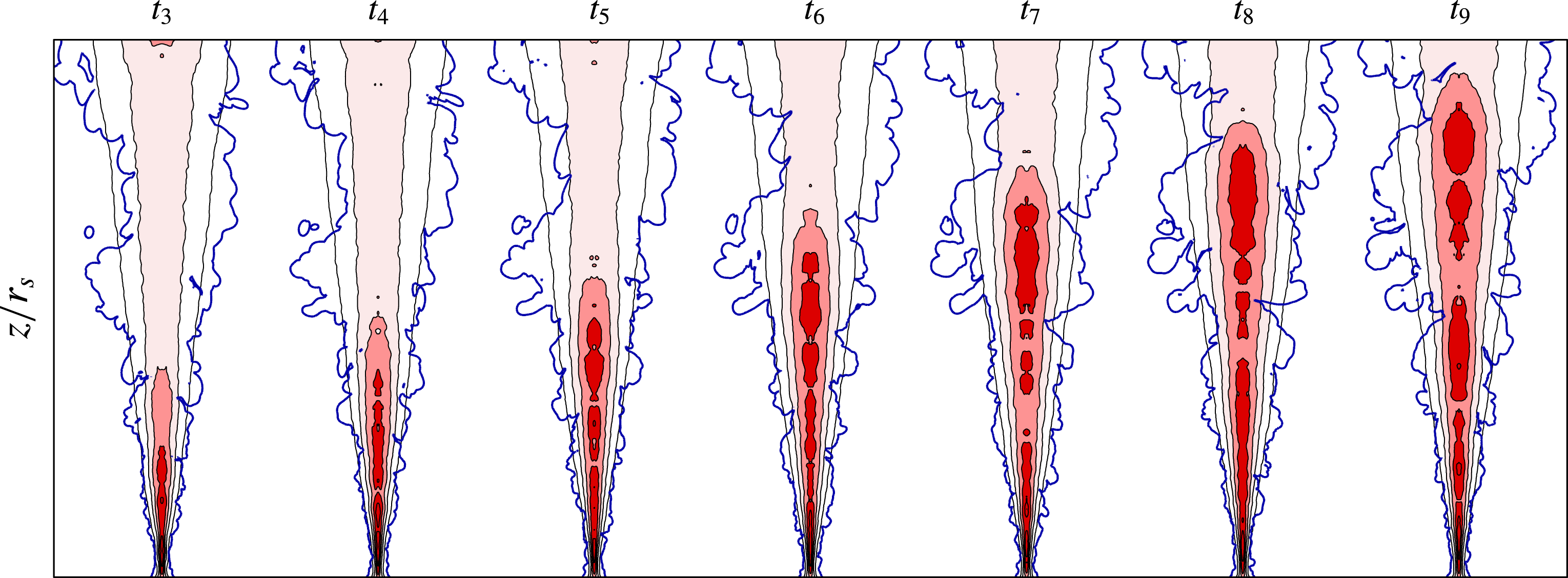
Figure 2. Isoregions of the ensemble and azimuthally averaged buoyancy (red) and threshold of the instantaneous enstrophy (blue) in an unsteady turbulent plume at times $t_{n}\approx 1.95{\it\tau}_{s}n$
,
$t_{n}\approx 1.95{\it\tau}_{s}n$
, $n=3,\ldots ,9$
, where
$n=3,\ldots ,9$
, where ${\it\tau}_{s}\equiv r_{s}^{4/3}(F_{s}^{A})^{-1/3}$
. The buoyancy displayed in the figure has been non-dimensionalised using the local characteristic buoyancy scale
${\it\tau}_{s}\equiv r_{s}^{4/3}(F_{s}^{A})^{-1/3}$
. The buoyancy displayed in the figure has been non-dimensionalised using the local characteristic buoyancy scale $b_{m0}\equiv B_{0}M_{0}/Q_{0}^{2}$
of a steady plume with buoyancy flux
$b_{m0}\equiv B_{0}M_{0}/Q_{0}^{2}$
of a steady plume with buoyancy flux $F^{B}$
.
$F^{B}$
.
The unsteady plume is illustrated in figure 2, which displays the azimuthal and ensemble-averaged normalised buoyancy field at several time instances, in addition to the instantaneous boundary of the plume, corresponding to a single member of the ensemble. The normalised buoyancy field was obtained by dividing $\overline{b}$
by a characteristic steady-state buoyancy
$\overline{b}$
by a characteristic steady-state buoyancy $b_{m0}(z)\equiv B_{0}M_{0}/Q_{0}^{2}$
, based on observations from L (i.e. a steady plume with source buoyancy flux
$b_{m0}(z)\equiv B_{0}M_{0}/Q_{0}^{2}$
, based on observations from L (i.e. a steady plume with source buoyancy flux $F^{B}$
). The boundary of the plume is defined by an isoline associated with a relatively small value of enstrophy, and therefore separates turbulent and non-turbulent parts of the flow. In the averaged buoyancy field one observes a smoothly defined cigar-shaped region penetrating progressively further into the domain. Although the size of the region increases with respect to time, its shape is approximately invariant over the range of times displayed in figure 2. Looking at the buoyancy field and the boundary of the plume in figure 2, one does not get the impression that the width or radial extent of the plume is strongly affected by the step change in the buoyancy flux. In this regard, we note that experimental observations of a plume, whose source buoyancy flux was suddenly reduced at the source, suggested that such plumes become narrower in the vicinity of the step change (Scase et al.
Reference Scase, Caulfield and Dalziel2008). However, consistent with our interpretation of figure 2, the change in plume width is not readily discernible from the radial extent of the passive scalar field presented in figures 3 and 4 of Scase et al. (Reference Scase, Caulfield and Dalziel2008). Only by quantifying the width of the plume with a top-hat width based on the concentration of the passive scalar do Scase et al. (Reference Scase, Caulfield and Dalziel2008) find that the plume becomes narrower (figure 6 of their study). The interpretation and observed behaviour of the plume radius will be discussed in further detail below.
$F^{B}$
). The boundary of the plume is defined by an isoline associated with a relatively small value of enstrophy, and therefore separates turbulent and non-turbulent parts of the flow. In the averaged buoyancy field one observes a smoothly defined cigar-shaped region penetrating progressively further into the domain. Although the size of the region increases with respect to time, its shape is approximately invariant over the range of times displayed in figure 2. Looking at the buoyancy field and the boundary of the plume in figure 2, one does not get the impression that the width or radial extent of the plume is strongly affected by the step change in the buoyancy flux. In this regard, we note that experimental observations of a plume, whose source buoyancy flux was suddenly reduced at the source, suggested that such plumes become narrower in the vicinity of the step change (Scase et al.
Reference Scase, Caulfield and Dalziel2008). However, consistent with our interpretation of figure 2, the change in plume width is not readily discernible from the radial extent of the passive scalar field presented in figures 3 and 4 of Scase et al. (Reference Scase, Caulfield and Dalziel2008). Only by quantifying the width of the plume with a top-hat width based on the concentration of the passive scalar do Scase et al. (Reference Scase, Caulfield and Dalziel2008) find that the plume becomes narrower (figure 6 of their study). The interpretation and observed behaviour of the plume radius will be discussed in further detail below.
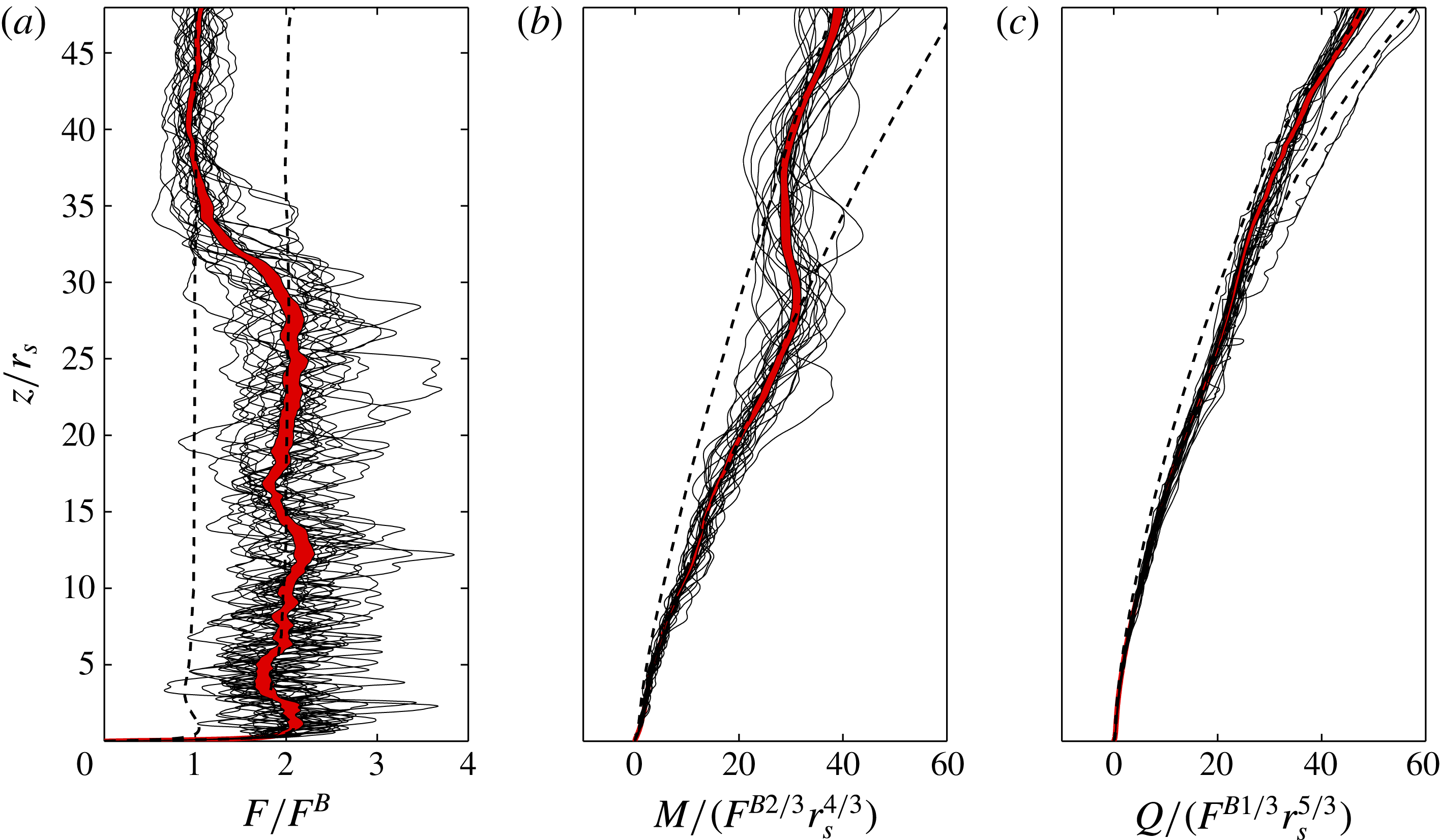
Figure 3. (a) Dimensionless buoyancy flux, (b) dimensionless momentum flux and (c) dimensionless volume flux, corresponding to individual members of the ensemble (thin lines) and their ensemble average (thick line) at $t/{\it\tau}_{s}=16$
. The width of the line denoting the ensemble average is equal to twice the standard deviation of the sample, divided by
$t/{\it\tau}_{s}=16$
. The width of the line denoting the ensemble average is equal to twice the standard deviation of the sample, divided by $\sqrt{n}$
, where
$\sqrt{n}$
, where $n=24$
is the number of members of the ensemble. The dashed lines correspond to steady-state data before and after the step change in the source buoyancy flux.
$n=24$
is the number of members of the ensemble. The dashed lines correspond to steady-state data before and after the step change in the source buoyancy flux.
The primary focus of this study is the behaviour of integral quantities such as the volume flux, mean momentum flux and the mean buoyancy flux. Figure 3 displays the longitudinal dependence of these quantities some time after the step change in the buoyancy flux at the source. To begin, we choose to display the mean buoyancy flux $F$
, rather than the integral buoyancy
$F$
, rather than the integral buoyancy $B$
, in figure 3. Being equal to the constants
$B$
, in figure 3. Being equal to the constants $F^{A}$
and
$F^{A}$
and $F^{B}$
upstream and downstream of the travelling wave respectively, the behaviour of the mean buoyancy flux is easier to interpret than that of the integral buoyancy. Integrals from each member of the ensemble show significant variation in comparison with the relatively smooth profile that is obtained from their ensemble average. In the mean buoyancy flux
$F^{B}$
upstream and downstream of the travelling wave respectively, the behaviour of the mean buoyancy flux is easier to interpret than that of the integral buoyancy. Integrals from each member of the ensemble show significant variation in comparison with the relatively smooth profile that is obtained from their ensemble average. In the mean buoyancy flux $F$
the step change has propagated to approximately
$F$
the step change has propagated to approximately $z/r_{s}=30$
. Since
$z/r_{s}=30$
. Since $F$
appears as a forcing term in the governing differential equation for the momentum flux
$F$
appears as a forcing term in the governing differential equation for the momentum flux $M$
, which is an integral of
$M$
, which is an integral of $\overline{w}^{2}$
rather than
$\overline{w}^{2}$
rather than $\overline{w}$
, one observes that the behaviour of
$\overline{w}$
, one observes that the behaviour of $Q$
is generally smoother than
$Q$
is generally smoother than $F$
and
$F$
and $M$
, making the step change in figure 3(c) comparatively difficult to discern.
$M$
, making the step change in figure 3(c) comparatively difficult to discern.
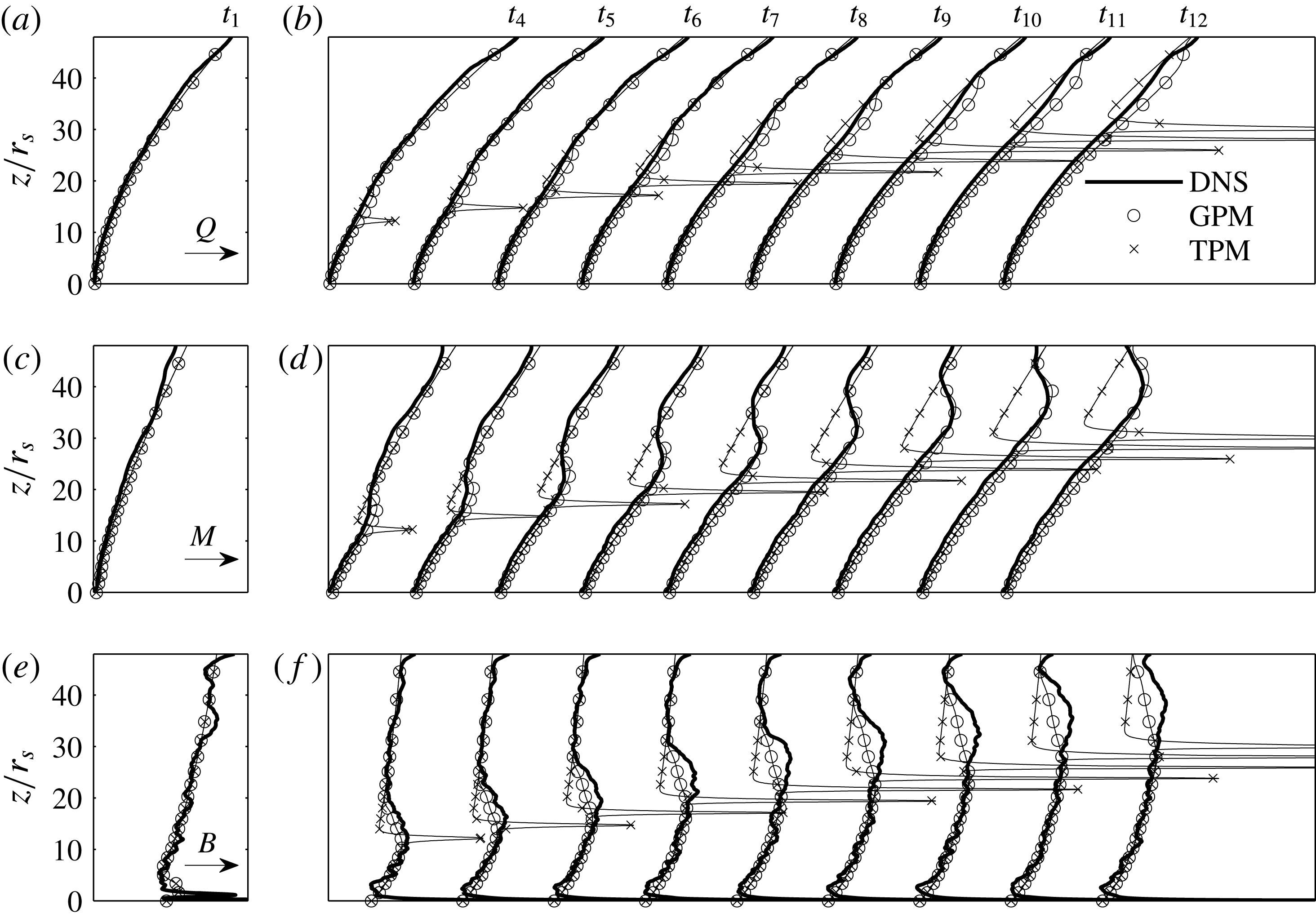
Figure 4. DNS data and model prediction of the volume flux $Q$
(a,b); the momentum flux
$Q$
(a,b); the momentum flux $M$
(c,d); and the integral buoyancy
$M$
(c,d); and the integral buoyancy $B$
(e,f). (a,c,e) Display the initial conditions, while (b,d,f) display the data/predictions at times
$B$
(e,f). (a,c,e) Display the initial conditions, while (b,d,f) display the data/predictions at times $t_{n}\approx 1.95{\it\tau}_{s}n$
. The thick solid line corresponds to the DNS data. GPM refers to the Gaussian plume model described in § 6 of this paper, while TPM refers to the top-hat plume model described by Scase & Hewitt (Reference Scase and Hewitt2012).
$t_{n}\approx 1.95{\it\tau}_{s}n$
. The thick solid line corresponds to the DNS data. GPM refers to the Gaussian plume model described in § 6 of this paper, while TPM refers to the top-hat plume model described by Scase & Hewitt (Reference Scase and Hewitt2012).
In figure 4 we examine the volume flux $Q$
, the momentum flux
$Q$
, the momentum flux $M$
and the integral buoyancy
$M$
and the integral buoyancy $B$
, which are the dependent variables of the system (2.9)–(2.11). The thick black lines correspond to data obtained from the simulation at a given time. Figure 4 also includes model predictions, which will be discussed in § 6. In each variable, one can observe a wave that travels in the direction of positive
$B$
, which are the dependent variables of the system (2.9)–(2.11). The thick black lines correspond to data obtained from the simulation at a given time. Figure 4 also includes model predictions, which will be discussed in § 6. In each variable, one can observe a wave that travels in the direction of positive $z$
for increasing
$z$
for increasing $t$
. As one would expect, knowing that the plume is driven by buoyancy, the position of the wave is approximately the same in each of the dependent variables. At a given time, upstream and downstream of the wave, the integrals
$t$
. As one would expect, knowing that the plume is driven by buoyancy, the position of the wave is approximately the same in each of the dependent variables. At a given time, upstream and downstream of the wave, the integrals $Q$
,
$Q$
, $M$
and
$M$
and $B$
satisfy a quasi-steady balance, and therefore the classical power-law solutions
$B$
satisfy a quasi-steady balance, and therefore the classical power-law solutions $B\sim z^{1/3}$
,
$B\sim z^{1/3}$
, $M\sim z^{4/3}$
and
$M\sim z^{4/3}$
and $Q\sim z^{5/3}$
are valid (cf. the dashed lines in figure 3),
$Q\sim z^{5/3}$
are valid (cf. the dashed lines in figure 3), $F_{s}$
in (2.22) being given by either
$F_{s}$
in (2.22) being given by either $F_{s}^{A}$
(upstream) or
$F_{s}^{A}$
(upstream) or $F_{s}^{B}$
(downstream) accordingly. In figure 4(b) and (f) for
$F_{s}^{B}$
(downstream) accordingly. In figure 4(b) and (f) for $z/r_{s}>42$
one can discern a small increase in
$z/r_{s}>42$
one can discern a small increase in $Q$
and
$Q$
and $B$
, respectively. The outflow boundary condition we employ results in an increase in
$B$
, respectively. The outflow boundary condition we employ results in an increase in $r_{d}$
just beneath the top of the domain, and therefore a corresponding increase in
$r_{d}$
just beneath the top of the domain, and therefore a corresponding increase in $Q$
and
$Q$
and $B$
(note that, being proportional to
$B$
(note that, being proportional to $\overline{w}^{2}$
, rather than
$\overline{w}^{2}$
, rather than $\overline{w}$
, the momentum flux
$\overline{w}$
, the momentum flux $M$
is not affected). In the case of
$M$
is not affected). In the case of $B$
, it is evident that the effects of the outflow are small in comparison with the amplitude of the travelling wave.
$B$
, it is evident that the effects of the outflow are small in comparison with the amplitude of the travelling wave.
The wave is perhaps most clearly seen in the integral buoyancy $B$
, which typically has a relatively weak power-law dependence on
$B$
, which typically has a relatively weak power-law dependence on $z$
. To within a constant rescaling factor, the longitudinal dependence of the integrals does not appear to alter significantly with respect to time. For example, the
$z$
. To within a constant rescaling factor, the longitudinal dependence of the integrals does not appear to alter significantly with respect to time. For example, the $z$
-dependence of
$z$
-dependence of $B(z,t_{10})$
is qualitatively similar to that of
$B(z,t_{10})$
is qualitatively similar to that of $B(z,t_{4})$
, if a suitable rescaling is applied. Although the main focus of this study is on the integrals
$B(z,t_{4})$
, if a suitable rescaling is applied. Although the main focus of this study is on the integrals $Q$
,
$Q$
, $M$
and
$M$
and $B$
, we note for future reference that the pressure integral
$B$
, we note for future reference that the pressure integral ${\it\beta}_{p}M$
warrants further attention. As one might expect, the dimensionless pressure integral
${\it\beta}_{p}M$
warrants further attention. As one might expect, the dimensionless pressure integral ${\it\beta}_{p}$
increases at the leading edge of the travelling wave and is therefore expected to influence the dynamics of the wave. Further understanding of this aspect of the flow would require a detailed analysis of the lateral components of the turbulence kinetic energy and are beyond the scope of this paper.
${\it\beta}_{p}$
increases at the leading edge of the travelling wave and is therefore expected to influence the dynamics of the wave. Further understanding of this aspect of the flow would require a detailed analysis of the lateral components of the turbulence kinetic energy and are beyond the scope of this paper.
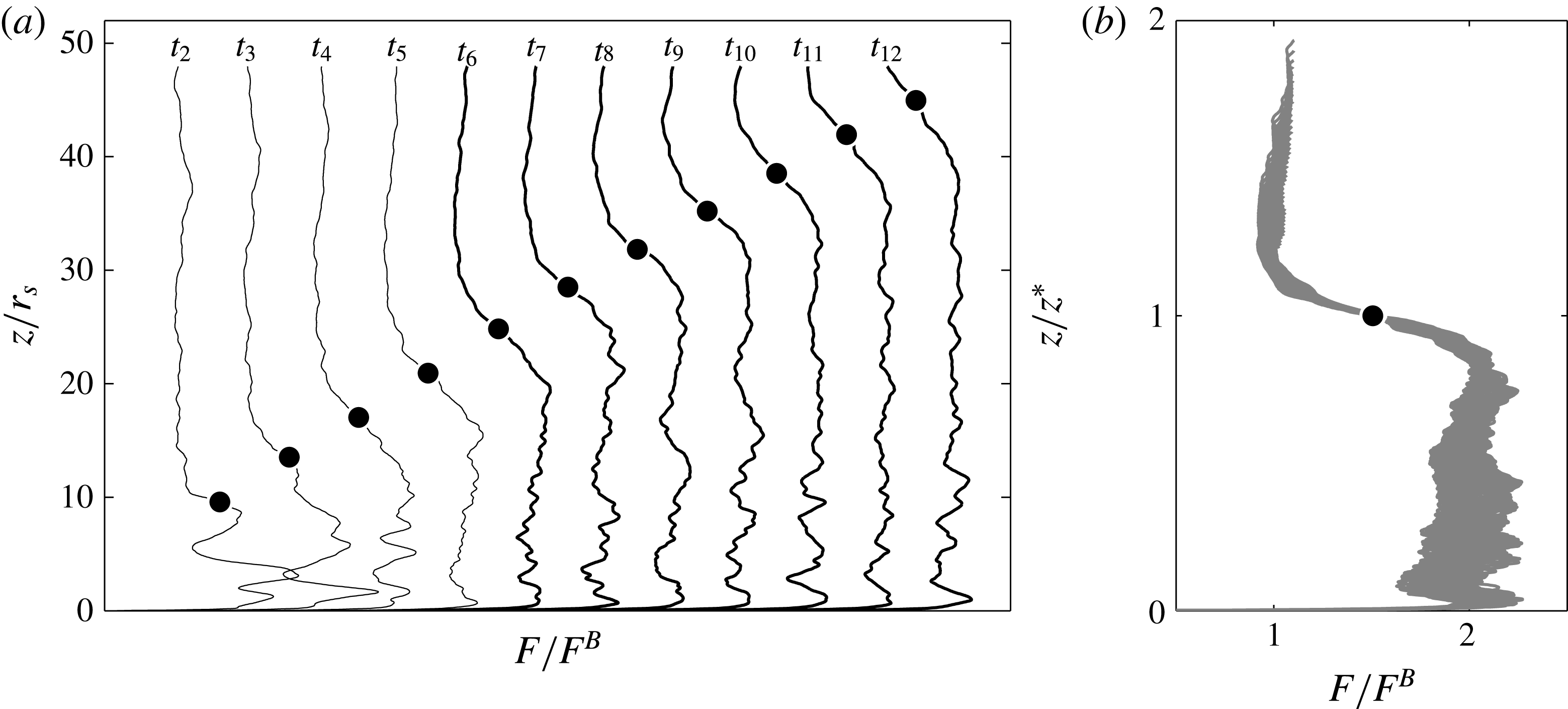
Figure 5. (a) Normalised buoyancy flux at the times $t_{n}\approx 1.95{\it\tau}_{s}n$
. The black circle denotes
$t_{n}\approx 1.95{\it\tau}_{s}n$
. The black circle denotes $z^{\ast }(t)$
, which corresponds to the location of the wave. Profiles
$z^{\ast }(t)$
, which corresponds to the location of the wave. Profiles $t_{2},\ldots ,t_{5}$
appear to be influenced by near-field effects and are therefore excluded from the plot in (b), which illustrates the self-similarity of the normalised buoyancy flux.
$t_{2},\ldots ,t_{5}$
appear to be influenced by near-field effects and are therefore excluded from the plot in (b), which illustrates the self-similarity of the normalised buoyancy flux.
Based on the behaviour of the dependent variables evident in figure 4, one wishes to understand the scaling associated with the travelling wave. To this end, we consider the buoyancy flux $F$
in figure 5(a) at several time instances. Being constant upstream and downstream of the wave, the buoyancy flux is a convenient variable to analyse in this regard. We now turn our attention to the scaling of the position of the step change
$F$
in figure 5(a) at several time instances. Being constant upstream and downstream of the wave, the buoyancy flux is a convenient variable to analyse in this regard. We now turn our attention to the scaling of the position of the step change $z^{\ast }(t)$
, leading eventually to the collapsed data from several time instances that is plotted with respect to the similarity variable
$z^{\ast }(t)$
, leading eventually to the collapsed data from several time instances that is plotted with respect to the similarity variable $z/z^{\ast }$
in figure 5(b).
$z/z^{\ast }$
in figure 5(b).
Using the integrals (2.12), it is useful to define the following characteristic length, velocity and buoyancy scales respectively:
 $$\begin{eqnarray}r_{m}\equiv \frac{Q}{M^{1/2}},\quad w_{m}\equiv \frac{M}{Q},\quad b_{m}\equiv \frac{BM}{Q^{2}}.\end{eqnarray}$$
Thus, according to classical plume theory (2.22), when ${\it\theta}_{m}={\it\beta}_{g}=1$
, the characteristic velocity in a steady plume, whose physical source is located at
${\it\theta}_{m}={\it\beta}_{g}=1$
, the characteristic velocity in a steady plume, whose physical source is located at $z=0$
, is
$z=0$
, is
 $$\begin{eqnarray}w_{m}=\frac{3}{4}\left(\frac{10}{9{\it\alpha}_{0}}\right)^{2/3}\left(\frac{F}{z-z_{v}}\right)^{1/3},\end{eqnarray}$$
where $z_{v}$
is the location of an asymptotic virtual source. One therefore presumes that, sufficiently far from the finite source, the location
$z_{v}$
is the location of an asymptotic virtual source. One therefore presumes that, sufficiently far from the finite source, the location $z^{\ast }$
of the propagating wave obeys
$z^{\ast }$
of the propagating wave obeys
 $$\begin{eqnarray}\frac{\text{d}z^{\ast }}{\text{d}t}={\it\lambda}^{\ast }w_{m}=\frac{3{\it\lambda}^{\ast }}{4}\left(\frac{10}{9{\it\alpha}_{0}}\right)^{2/3}\left(\frac{F^{\ast }}{z^{\ast }-z_{v}}\right)^{1/3},\end{eqnarray}$$
where ${\it\lambda}^{\ast }$
is a constant of proportionality and
${\it\lambda}^{\ast }$
is a constant of proportionality and $F^{\ast }$
is a characteristic buoyancy flux such that
$F^{\ast }$
is a characteristic buoyancy flux such that $F^{B}\leqslant F^{\ast }\leqslant F^{A}$
. We define the characteristic buoyancy flux by imposing buoyancy conservation in the wave and solving the corresponding Rankine–Hugoniot jump conditions, as outlined in appendix C:
$F^{B}\leqslant F^{\ast }\leqslant F^{A}$
. We define the characteristic buoyancy flux by imposing buoyancy conservation in the wave and solving the corresponding Rankine–Hugoniot jump conditions, as outlined in appendix C:
 $$\begin{eqnarray}F^{\ast }\equiv \frac{8}{27}\left(\frac{F^{A}-F^{B}}{(F^{A})^{2/3}-(F^{B})^{2/3}}\right)^{3}.\end{eqnarray}$$
As one would expect, (4.4) implies that for infinitesimal changes in $F$
,
$F$
, $F^{\ast }\sim F^{A}\sim F^{B}$
.
$F^{\ast }\sim F^{A}\sim F^{B}$
.
One can integrate equation (4.3) to find that
 $$\begin{eqnarray}(z^{\ast }-z_{v})^{4/3}={\it\lambda}^{\ast }\left(\frac{10}{9{\it\alpha}_{0}}\right)^{2/3}F^{\ast \,1/3}(t-t_{v}),\end{eqnarray}$$
where $t_{v}$
is the time for which
$t_{v}$
is the time for which $z^{\ast }(t_{v})=z_{v}$
.
$z^{\ast }(t_{v})=z_{v}$
.
We determine $z^{\ast }(t)$
from the DNS data in a simple and reliable manner according to
$z^{\ast }(t)$
from the DNS data in a simple and reliable manner according to
 $$\begin{eqnarray}F(z^{\ast }(t),t)=F^{\ast }.\end{eqnarray}$$
Consequently, if $F$
is monotonic, according to (4.6)
$F$
is monotonic, according to (4.6) $z^{\ast }$
is single-valued function of time. To ensure a unique definition of
$z^{\ast }$
is single-valued function of time. To ensure a unique definition of $z^{\ast }$
in situations in which
$z^{\ast }$
in situations in which $F$
is not monotonic, we take the maximum value of
$F$
is not monotonic, we take the maximum value of $z^{\ast }$
satisfying (4.6). With the exception of a small region in the near field (see
$z^{\ast }$
satisfying (4.6). With the exception of a small region in the near field (see $t_{2}$
and
$t_{2}$
and $t_{3}$
in figure 5), we find that (4.6) is sufficient in defining a unique value of
$t_{3}$
in figure 5), we find that (4.6) is sufficient in defining a unique value of $z^{\ast }$
. The position
$z^{\ast }$
. The position $z^{\ast }(t)$
, determined according to (4.6), is displayed in figure 5(a) with respect to the buoyancy flux at several time instances and evidently provides a useful indication of the wave’s position. In figure 5(b) we rescale the longitudinal coordinate
$z^{\ast }(t)$
, determined according to (4.6), is displayed in figure 5(a) with respect to the buoyancy flux at several time instances and evidently provides a useful indication of the wave’s position. In figure 5(b) we rescale the longitudinal coordinate $z$
using the observed front position
$z$
using the observed front position $z^{\ast }(t)$
. Plotting the mean buoyancy flux
$z^{\ast }(t)$
. Plotting the mean buoyancy flux $F$
at times
$F$
at times $t\geqslant t_{6}$
with respect to
$t\geqslant t_{6}$
with respect to $z/z^{\ast }$
, we observe an approximate collapse of the data and therefore self-similarity. Here, self-similarity implies that sufficiently far from the source (or, equivalently, at sufficiently large times) the process reaches a state of ‘equilibrium’ in which
$z/z^{\ast }$
, we observe an approximate collapse of the data and therefore self-similarity. Here, self-similarity implies that sufficiently far from the source (or, equivalently, at sufficiently large times) the process reaches a state of ‘equilibrium’ in which $z$
and
$z$
and $t$
cease to play independent roles. We also note that if
$t$
cease to play independent roles. We also note that if $z^{\ast }\sim t^{3/4}$
then self-similarity implies that the longitudinal extent (i.e. the spreading rate) of the front also scales according to
$z^{\ast }\sim t^{3/4}$
then self-similarity implies that the longitudinal extent (i.e. the spreading rate) of the front also scales according to $t^{3/4}$
. For small times (see
$t^{3/4}$
. For small times (see $t_{2}$
,
$t_{2}$
, $t_{3}$
and
$t_{3}$
and $t_{4}$
in figure 5(a)) we observe that the disturbance in the buoyancy flux is oscillatory and that the local peak in the buoyancy flux at approximately
$t_{4}$
in figure 5(a)) we observe that the disturbance in the buoyancy flux is oscillatory and that the local peak in the buoyancy flux at approximately $z/r_{s}=9$
breaks down before
$z/r_{s}=9$
breaks down before $t_{4}$
and results in a significant reduction in the steepness of the wave. Consequently, between
$t_{4}$
and results in a significant reduction in the steepness of the wave. Consequently, between $t_{3}$
and
$t_{3}$
and $t_{6}$
the wave front appears to become steeper as it adjusts to a far-field equilibrium.
$t_{6}$
the wave front appears to become steeper as it adjusts to a far-field equilibrium.

Figure 6. Dimensionless buoyancy $b_{m}(z,t)/b_{m0}(z)$
in the plume, where
$b_{m}(z,t)/b_{m0}(z)$
in the plume, where $b_{m0}$
is the steady-state buoyancy corresponding to simulation L with buoyancy flux
$b_{m0}$
is the steady-state buoyancy corresponding to simulation L with buoyancy flux $F^{B}$
, in addition to points denoting the location of the travelling wave. The crosses correspond to the observed position of the front, while the line denotes a best fit to the front position, of the form
$F^{B}$
, in addition to points denoting the location of the travelling wave. The crosses correspond to the observed position of the front, while the line denotes a best fit to the front position, of the form $z^{\ast }-z_{v}\propto (t-t_{v})^{3/4}$
.
$z^{\ast }-z_{v}\propto (t-t_{v})^{3/4}$
.
In figure 6 we test the hypothesis that $z^{\ast }\sim t^{3/4}$
and determine the constant of proportionality
$z^{\ast }\sim t^{3/4}$
and determine the constant of proportionality ${\it\lambda}^{\ast }$
from the observed location of the front
${\it\lambda}^{\ast }$
from the observed location of the front $z^{\ast }(t)$
. Evident from the normalised characteristic buoyancy
$z^{\ast }(t)$
. Evident from the normalised characteristic buoyancy $b_{m}/b_{m0}$
displayed in figure 6 is that in the far field the wave’s propagation adheres to the predicted
$b_{m}/b_{m0}$
displayed in figure 6 is that in the far field the wave’s propagation adheres to the predicted $z^{\ast }\sim t^{3/4}$
scaling. In addition, we find that the constant of proportionality
$z^{\ast }\sim t^{3/4}$
scaling. In addition, we find that the constant of proportionality ${\it\lambda}^{\ast }\approx 1.9$
in (4.5). In other words, with reference to (4.3), we observe that the front propagates at nearly twice the local top-hat velocity
${\it\lambda}^{\ast }\approx 1.9$
in (4.5). In other words, with reference to (4.3), we observe that the front propagates at nearly twice the local top-hat velocity $w_{m}$
. This behaviour is consistent with unsteady turbulent jets (Craske & van Reeuwijk Reference Craske and van Reeuwijk2015a
), and will be explained in § 5 in terms of the dimensionless profile coefficients.
$w_{m}$
. This behaviour is consistent with unsteady turbulent jets (Craske & van Reeuwijk Reference Craske and van Reeuwijk2015a
), and will be explained in § 5 in terms of the dimensionless profile coefficients.
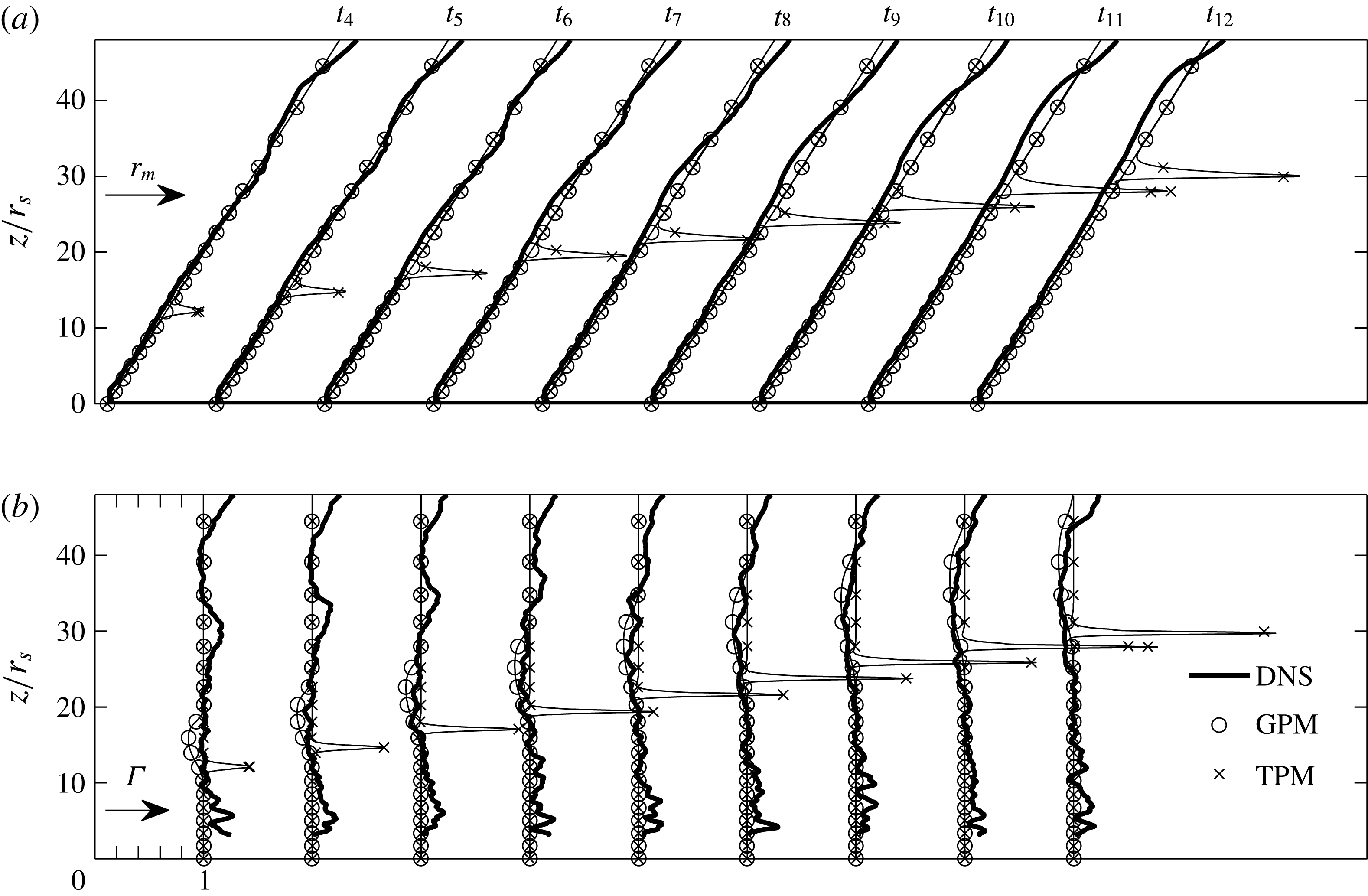
Figure 7. DNS data and model prediction of the plume radius $r_{m}$
(a) and the flux-balance parameter
$r_{m}$
(a) and the flux-balance parameter ${\it\Gamma}$
(b) at times
${\it\Gamma}$
(b) at times $t_{n}\approx 1.95{\it\tau}_{s}n$
. The thick solid line corresponds to the DNS data. GPM refers to the Gaussian plume model described in § 6 of this paper and TPM refers to the top-hat plume model described by Scase & Hewitt (Reference Scase and Hewitt2012). Note that the profiles in (b) are separated by a distance of 1 unit, as indicated by the scale in the bottom left corner.
$t_{n}\approx 1.95{\it\tau}_{s}n$
. The thick solid line corresponds to the DNS data. GPM refers to the Gaussian plume model described in § 6 of this paper and TPM refers to the top-hat plume model described by Scase & Hewitt (Reference Scase and Hewitt2012). Note that the profiles in (b) are separated by a distance of 1 unit, as indicated by the scale in the bottom left corner.
Compared with $Q$
,
$Q$
, $M$
and
$M$
and $B$
, it is perhaps the derived quantities
$B$
, it is perhaps the derived quantities $r_{m}\equiv Q/M^{1/2}$
and
$r_{m}\equiv Q/M^{1/2}$
and ${\it\Gamma}\propto QB/M^{3/2}$
that reveal more about the dynamics of the system, because, unlike
${\it\Gamma}\propto QB/M^{3/2}$
that reveal more about the dynamics of the system, because, unlike $Q$
,
$Q$
, $M$
and
$M$
and $B$
, the characteristic plume radius
$B$
, the characteristic plume radius $r_{m}$
and flux-balance parameter
$r_{m}$
and flux-balance parameter ${\it\Gamma}$
are independent of
${\it\Gamma}$
are independent of $F$
. Without scrutinising the governing equations, it is therefore difficult to predict whether
$F$
. Without scrutinising the governing equations, it is therefore difficult to predict whether $r_{m}$
and
$r_{m}$
and ${\it\Gamma}$
will increase or decrease in the vicinity of the propagating wave. Figure 7 demonstrates that to leading-order, the behaviour of
${\it\Gamma}$
will increase or decrease in the vicinity of the propagating wave. Figure 7 demonstrates that to leading-order, the behaviour of $r_{m}$
and
$r_{m}$
and ${\it\Gamma}$
is practically unaffected by the step change in the buoyancy flux. One is inclined to conclude that
${\it\Gamma}$
is practically unaffected by the step change in the buoyancy flux. One is inclined to conclude that $r_{m}$
and
$r_{m}$
and ${\it\Gamma}$
are slightly reduced in the vicinity of the wave although the observed change, being not more than 15 % of their steady-state values, is relatively small. We will discuss the physics determining the behaviour of
${\it\Gamma}$
are slightly reduced in the vicinity of the wave although the observed change, being not more than 15 % of their steady-state values, is relatively small. We will discuss the physics determining the behaviour of $r_{m}$
and
$r_{m}$
and ${\it\Gamma}$
in §§ 5.2–5.3 and demonstrate why they are only weakly sensitive to changes in the plume’s buoyancy flux.
${\it\Gamma}$
in §§ 5.2–5.3 and demonstrate why they are only weakly sensitive to changes in the plume’s buoyancy flux.
5 Unsteady plume properties
To understand the leading-order role played by the profile coefficients in the unsteady plume equations (2.9)–(2.11), we will start by assuming that they are constants. Consideration of the possibility that, for example, the dimensionless buoyancy flux changes in the vicinity of the front is addressed in § 6.1. In § 2 we described a framework that postpones making assumptions about unknown quantities such as turbulent fluxes, pressure and the radial dependence of the velocity profile. The framework therefore allows one to investigate and understand how assumptions about the flow from an integral perspective affect the structure of a generalised system of governing equations.
5.1 The hyperbolic system
A logical starting point to understand the leading-order physics associated with the system (2.9)–(2.11) is to analyse its characteristic curves. Without assigning a value to the profile coefficients ${\it\beta}_{g}$
,
${\it\beta}_{g}$
, ${\it\gamma}_{g}$
and
${\it\gamma}_{g}$
and ${\it\theta}_{g}$
, which correspond to dimensionless fluxes of momentum, energy and buoyancy, respectively, the unsteady plume equations can be expressed as
${\it\theta}_{g}$
, which correspond to dimensionless fluxes of momentum, energy and buoyancy, respectively, the unsteady plume equations can be expressed as
 $$\begin{eqnarray}\left\{\frac{\partial }{\partial t}+\left[\begin{array}{@{}ccc@{}}0 & {\it\beta}_{g} & 0\\ -{\it\gamma}_{g}{\displaystyle \frac{M^{2}}{Q^{2}}} & {\it\gamma}_{g}{\displaystyle \frac{2M}{Q}} & 0\\ -{\it\theta}_{g}{\displaystyle \frac{BM}{Q^{2}}} & {\it\theta}_{g}{\displaystyle \frac{B}{Q}} & {\it\theta}_{g}{\displaystyle \frac{M}{Q}}\end{array}\right]\frac{\partial }{\partial z}\right\}\left(\begin{array}{@{}c@{}}Q\\ M\\ B\end{array}\right)=\boldsymbol{R},\end{eqnarray}$$
where $\boldsymbol{R}$
consists of the right-hand side sink or source terms appearing in (2.9)–(2.11). Characteristic curves of this system satisfy the following relation
$\boldsymbol{R}$
consists of the right-hand side sink or source terms appearing in (2.9)–(2.11). Characteristic curves of this system satisfy the following relation
 $$\begin{eqnarray}\det \left[\begin{array}{@{}ccc@{}}-{\it\lambda}^{\ast } & {\it\beta}_{g}{\displaystyle \frac{Q}{M}} & 0\\ -{\it\gamma}_{g}{\displaystyle \frac{M}{Q}} & 2{\it\gamma}_{g}-{\it\lambda}^{\ast } & 0\\ -{\it\theta}_{g}{\displaystyle \frac{B}{Q}} & {\it\theta}_{g}{\displaystyle \frac{B}{M}} & {\it\theta}_{g}-{\it\lambda}^{\ast }\end{array}\right]=0,\end{eqnarray}$$
where ${\it\lambda}^{\ast }$
is a dimensionless velocity defined by
${\it\lambda}^{\ast }$
is a dimensionless velocity defined by
 $$\begin{eqnarray}{\it\lambda}^{\ast }\equiv \frac{\text{d}z}{\text{d}t}\frac{Q}{M}.\end{eqnarray}$$
The relation (5.2) implies that
 $$\begin{eqnarray}{\it\lambda}^{\ast }=\left\{\begin{array}{@{}l@{}}{\it\lambda}_{1}={\it\gamma}_{g}+\sqrt{{\it\gamma}_{g}^{2}-{\it\gamma}_{g}{\it\beta}_{g}},\quad \\ {\it\lambda}_{2}={\it\theta}_{g},\quad \\ {\it\lambda}_{3}={\it\gamma}_{g}-\sqrt{{\it\gamma}_{g}^{2}-{\it\gamma}_{g}{\it\beta}_{g}}.\quad \end{array}\right.\end{eqnarray}$$
To date, the assumption of top-hat velocity profiles and the omission of turbulence has resulted in the unsteady plume equations being regarded as a parabolic system (Scase et al.
Reference Scase, Aspden and Caulfield2009). However, use of the generalised framework described in § 2 reveals that, in general, the unsteady plume equations comprise a hyperbolic system, even when higher-order turbulent transport terms are neglected from (2.6) and (2.8) (resulting in ${\it\beta}_{g}={\it\beta}_{m}$
and
${\it\beta}_{g}={\it\beta}_{m}$
and ${\it\gamma}_{g}={\it\gamma}_{m}$
). Evident from (5.4) is that in the ‘top-hat’ limit,
${\it\gamma}_{g}={\it\gamma}_{m}$
). Evident from (5.4) is that in the ‘top-hat’ limit, ${\it\gamma}_{g},{\it\beta}_{g},{\it\theta}_{g}\rightarrow 1$
,
${\it\gamma}_{g},{\it\beta}_{g},{\it\theta}_{g}\rightarrow 1$
, ${\it\lambda}^{\ast }=1$
, the characteristic curves collapse onto a single family propagating at the local characteristic velocity. In that case, the system cannot be decomposed using linearly independent eigenvectors and should indeed be regarded as parabolic (see Whitham Reference Whitham1974). The top-hat unsteady plume formulation is therefore a degenerate case amongst a wide variety of possible alternatives, each possessing quite different dynamical properties and underlying physics. In fact, top-hat models represent a non-physical limit in the sense that a discontinuous mean velocity field is not realisable in a real turbulent plume. However, we would like to point out that in comparing the radial dependence of different velocity profiles in the light of (5.4) one is not interested in whether they possess compact support per se, but in the extent to which they are non-uniform and/or account for turbulence and pressure. As described in § 2.3, a non-uniform radial dependence of longitudinal velocity always results in a higher dimensionless energy flux
${\it\lambda}^{\ast }=1$
, the characteristic curves collapse onto a single family propagating at the local characteristic velocity. In that case, the system cannot be decomposed using linearly independent eigenvectors and should indeed be regarded as parabolic (see Whitham Reference Whitham1974). The top-hat unsteady plume formulation is therefore a degenerate case amongst a wide variety of possible alternatives, each possessing quite different dynamical properties and underlying physics. In fact, top-hat models represent a non-physical limit in the sense that a discontinuous mean velocity field is not realisable in a real turbulent plume. However, we would like to point out that in comparing the radial dependence of different velocity profiles in the light of (5.4) one is not interested in whether they possess compact support per se, but in the extent to which they are non-uniform and/or account for turbulence and pressure. As described in § 2.3, a non-uniform radial dependence of longitudinal velocity always results in a higher dimensionless energy flux ${\it\gamma}_{m}$
, and therefore a separation of characteristic curves, and an unsteady equation for the area of the plume (2.19) that is fundamentally different from that which is associated with top-hat velocity profiles.
${\it\gamma}_{m}$
, and therefore a separation of characteristic curves, and an unsteady equation for the area of the plume (2.19) that is fundamentally different from that which is associated with top-hat velocity profiles.
A leading-order representation of a Gaussian unsteady plume is obtained by neglecting turbulent transport (hence ${\it\beta}_{g}=1$
,
${\it\beta}_{g}=1$
, ${\it\theta}_{g}=1$
and
${\it\theta}_{g}=1$
and ${\it\gamma}_{g}={\it\gamma}_{m}$
), and using the fact that
${\it\gamma}_{g}={\it\gamma}_{m}$
), and using the fact that ${\it\gamma}_{m}=4/3$
, as shown in (2.18). Consequently, (5.4) shows that for Gaussian profiles
${\it\gamma}_{m}=4/3$
, as shown in (2.18). Consequently, (5.4) shows that for Gaussian profiles ${\it\lambda}_{1}=2$
, which implies that the fastest characteristic propagates at twice the local characteristic velocity. This prediction is in reasonably close agreement with the observations reported in § 4 which suggest that
${\it\lambda}_{1}=2$
, which implies that the fastest characteristic propagates at twice the local characteristic velocity. This prediction is in reasonably close agreement with the observations reported in § 4 which suggest that ${\it\lambda}^{\ast }\approx 1.9$
. We tentatively attribute the fact that the observed propagation velocity is slightly less than one would expect to find in a Gaussian plume (
${\it\lambda}^{\ast }\approx 1.9$
. We tentatively attribute the fact that the observed propagation velocity is slightly less than one would expect to find in a Gaussian plume ( ${\it\lambda}^{\ast }\approx 2.0$
) to pressure, which typically being negative inside the plume (see, e.g.
${\it\lambda}^{\ast }\approx 2.0$
) to pressure, which typically being negative inside the plume (see, e.g. ${\it\beta}_{p}$
and
${\it\beta}_{p}$
and ${\it\gamma}_{p}$
in table 2), leads to a reduction in both
${\it\gamma}_{p}$
in table 2), leads to a reduction in both ${\it\beta}_{g}$
and
${\it\beta}_{g}$
and ${\it\gamma}_{g}$
.
${\it\gamma}_{g}$
.
5.2 The behaviour of the plume radius and flux-balance parameter
As pointed out in § 4, it is difficult to predict the behaviour of the characteristic radius $r_{m}\equiv Q/M^{1/2}$
and the flux-balance parameter
$r_{m}\equiv Q/M^{1/2}$
and the flux-balance parameter ${\it\Gamma}$
, which are derived quantities, in an unsteady plume a priori. It is therefore useful to understand how their behaviour is affected by the value of the profile coefficients.
${\it\Gamma}$
, which are derived quantities, in an unsteady plume a priori. It is therefore useful to understand how their behaviour is affected by the value of the profile coefficients.
Substitution of the relation $Q=r_{m}M^{1/2}$
into (2.20), reveals that
$Q=r_{m}M^{1/2}$
into (2.20), reveals that
 $$\begin{eqnarray}\frac{1}{{\it\gamma}_{g}M^{1/2}}\frac{\partial r_{m}^{2}}{\partial t}=-\frac{{\it\delta}_{g}}{{\it\gamma}_{g}}+\frac{2r_{m}}{M}\left(\frac{3}{4}-\frac{{\it\beta}_{g}}{{\it\gamma}_{g}}\right)\frac{\partial M}{\partial z}+\frac{16{\it\alpha}_{0}}{5}\left(\frac{{\it\beta}_{g}}{{\it\gamma}_{g}}-\frac{{\it\beta}_{g}{\it\theta}_{m}}{{\it\gamma}_{g}}\right){\it\Gamma}-\frac{\partial r_{m}}{\partial z}.\end{eqnarray}$$
If one assumes that at a particular time the plume is straight sided (conical), such that $\partial _{z}r_{m}=6{\it\alpha}_{0}/5$
in the right-hand side of (5.5) then, using (2.23),
$\partial _{z}r_{m}=6{\it\alpha}_{0}/5$
in the right-hand side of (5.5) then, using (2.23),
 $$\begin{eqnarray}\frac{1}{{\it\gamma}_{g}M^{1/2}}\frac{\partial r_{m}^{2}}{\partial t}=\frac{2r_{m}}{M}\left(\frac{3}{4}-\frac{{\it\beta}_{g}}{{\it\gamma}_{g}}\right)\frac{\partial M}{\partial z}+\frac{12{\it\alpha}_{0}}{5}\left(\frac{4{\it\beta}_{g}}{3{\it\gamma}_{g}}({\it\theta}_{m}+(1-{\it\theta}_{m}){\it\Gamma})-1\right).\end{eqnarray}$$
Inspection of (5.6) implies that
 $$\begin{eqnarray}\frac{\partial r_{m}^{2}}{\partial t}=0\quad \forall \left({\it\Gamma},\frac{r_{m}}{M}\frac{\partial M}{\partial z}\right)\quad \text{if }\frac{3{\it\gamma}_{g}}{4{\it\beta}_{g}}=1,~\text{and }{\it\theta}_{m}=1.\end{eqnarray}$$
When the profile coefficients are such that (a) ${\it\gamma}_{g}/{\it\beta}_{g}=4/3$
and (b)
${\it\gamma}_{g}/{\it\beta}_{g}=4/3$
and (b) ${\it\theta}_{m}=1$
, the plume remains straight sided for all time, provided that it has a constant source area. Physically, these conditions correspond to (a) the gross dimensionless fluxes of energy and momentum in the plume being in the ratio of
${\it\theta}_{m}=1$
, the plume remains straight sided for all time, provided that it has a constant source area. Physically, these conditions correspond to (a) the gross dimensionless fluxes of energy and momentum in the plume being in the ratio of $4/3$
and (b) the mean dimensionless flux of buoyancy in the plume being equal to unity. The latter condition is satisfied if the mean buoyancy profile has the same shape and width as the mean velocity profile.
$4/3$
and (b) the mean dimensionless flux of buoyancy in the plume being equal to unity. The latter condition is satisfied if the mean buoyancy profile has the same shape and width as the mean velocity profile.
The difference between straight sidedness in jets (see Craske & van Reeuwijk Reference Craske and van Reeuwijk2015b
) and plumes is an additional, independent, condition on ${\it\theta}_{m}$
in the case of the latter. Indeed,
${\it\theta}_{m}$
in the case of the latter. Indeed, ${\it\theta}_{m}$
places further control on the behaviour of
${\it\theta}_{m}$
places further control on the behaviour of $\partial _{t}M$
relative to
$\partial _{t}M$
relative to $\partial _{t}Q$
(see (2.9)–(2.10)) and therefore affects the behaviour of
$\partial _{t}Q$
(see (2.9)–(2.10)) and therefore affects the behaviour of $Q^{2}/M$
. The relations (5.7) are useful because they allow one to relate the ‘internal’ properties of a plume, such as
$Q^{2}/M$
. The relations (5.7) are useful because they allow one to relate the ‘internal’ properties of a plume, such as ${\it\gamma}_{g}$
, to an ‘external’ observable such as
${\it\gamma}_{g}$
, to an ‘external’ observable such as $r_{m}$
at the integral level. This contrasts with steady-state plumes, for which it is not possible to distinguish between a Gaussian or a top-hat distribution of velocity by observing
$r_{m}$
at the integral level. This contrasts with steady-state plumes, for which it is not possible to distinguish between a Gaussian or a top-hat distribution of velocity by observing $Q,M$
and
$Q,M$
and $F$
.
$F$
.
If we assume that the conditions (5.7) for straight sidedness are satisfied, then, using (2.25),
 $$\begin{eqnarray}B=\frac{4{\it\beta}_{g}M}{3z}{\it\Gamma}.\end{eqnarray}$$
Substitution of (5.8) into (2.11) and using (2.10), in addition to ${\it\beta}_{g}=3{\it\gamma}_{g}/4$
,
${\it\beta}_{g}=3{\it\gamma}_{g}/4$
, ${\it\theta}_{m}=1$
for straight sidedness, one obtains
${\it\theta}_{m}=1$
for straight sidedness, one obtains
 $$\begin{eqnarray}\frac{\partial {\it\Gamma}}{\partial t}=0\quad \forall \frac{\partial M}{\partial z}\quad \text{if }{\it\theta}_{g}={\it\gamma}_{g}\end{eqnarray}$$
provided that ${\it\Gamma}=1\,\forall z$
is an initial condition and that
${\it\Gamma}=1\,\forall z$
is an initial condition and that ${\it\Gamma}=1$
at the source. Therefore, only if the gross dimensionless buoyancy flux
${\it\Gamma}=1$
at the source. Therefore, only if the gross dimensionless buoyancy flux ${\it\theta}_{g}$
(i.e. inclusive of turbulent transport) is equal to the gross dimensionless energy flux
${\it\theta}_{g}$
(i.e. inclusive of turbulent transport) is equal to the gross dimensionless energy flux ${\it\gamma}_{g}$
will the plume remain pure, such that
${\it\gamma}_{g}$
will the plume remain pure, such that ${\it\Gamma}=1$
, regardless of the temporal dependence of
${\it\Gamma}=1$
, regardless of the temporal dependence of $M(z,t)$
. Noting that
$M(z,t)$
. Noting that ${\it\theta}_{m}=1$
for straight sidedness and that
${\it\theta}_{m}=1$
for straight sidedness and that ${\it\gamma}_{g}\approx 4/3$
, it is only possible that
${\it\gamma}_{g}\approx 4/3$
, it is only possible that ${\it\theta}_{g}={\it\gamma}_{g}$
if approximately
${\it\theta}_{g}={\it\gamma}_{g}$
if approximately $1/4$
of the total buoyancy flux is transported by turbulence. Table 2 suggests that
$1/4$
of the total buoyancy flux is transported by turbulence. Table 2 suggests that ${\it\theta}_{g}\approx 1.2$
, while
${\it\theta}_{g}\approx 1.2$
, while ${\it\gamma}_{g}\approx 1.4$
, and therefore we would not expect for the plume to remain precisely pure. However, in situations for which the prediction of local changes in
${\it\gamma}_{g}\approx 1.4$
, and therefore we would not expect for the plume to remain precisely pure. However, in situations for which the prediction of local changes in ${\it\Gamma}$
is not crucial, the assumption of equality between
${\it\Gamma}$
is not crucial, the assumption of equality between ${\it\gamma}_{g}$
and
${\it\gamma}_{g}$
and ${\it\theta}_{g}$
will prove to be a useful idealisation in the context of modelling, which we discuss in § 6.
${\it\theta}_{g}$
will prove to be a useful idealisation in the context of modelling, which we discuss in § 6.
5.3 The structure of waves in a plume
The way in which the properties of travelling waves in the plume depend on the profile coefficients can be established by examining the behaviour of the invariants associated with (5.1). The left eigenvectors corresponding to the eigenvalues (5.4) are

where ${\it\phi}\equiv \sqrt{1-{\it\beta}_{g}/{\it\gamma}_{g}}$
,
${\it\phi}\equiv \sqrt{1-{\it\beta}_{g}/{\it\gamma}_{g}}$
,
 $$\begin{eqnarray}c_{1}\equiv {\displaystyle \frac{{\it\theta}_{g}({\it\gamma}_{g}-{\it\theta}_{g})}{{\it\beta}_{g}{\it\gamma}_{g}-2{\it\gamma}_{g}{\it\theta}_{g}+{\it\theta}_{g}^{2}}},\quad \text{and}\quad c_{2}\equiv {\displaystyle \frac{{\it\theta}_{g}({\it\beta}_{g}-{\it\theta}_{g})}{{\it\beta}_{g}{\it\gamma}_{g}-2{\it\gamma}_{g}{\it\theta}_{g}+{\it\theta}_{g}^{2}}}.\end{eqnarray}$$
In general, $L$
is invertible, which means that the unsteady plume system (5.1) can be decomposed into a system of ordinary differential equations. Each differential equation corresponds to the derivative of a quasi-invariant quantity
$L$
is invertible, which means that the unsteady plume system (5.1) can be decomposed into a system of ordinary differential equations. Each differential equation corresponds to the derivative of a quasi-invariant quantity $Y_{1},Y_{2}$
or
$Y_{1},Y_{2}$
or $Y_{3}$
along a characteristic curve. In particular, introducing the integrating factor
$Y_{3}$
along a characteristic curve. In particular, introducing the integrating factor $Q^{c_{1}}/M^{c_{2}}$
:
$Q^{c_{1}}/M^{c_{2}}$
:
 $$\begin{eqnarray}\text{d}Y_{2}=c_{1}\frac{BQ^{c_{1}-1}}{M^{c_{2}}}\,\text{d}Q-c_{2}\frac{BQ^{c_{1}}}{M^{c_{2}+1}}\,\text{d}M+\frac{Q^{c_{1}}}{M^{c_{2}}}\,\text{d}B,\end{eqnarray}$$
one finds that
 $$\begin{eqnarray}Y_{2}=\frac{BQ^{c_{1}}}{M^{c_{2}}}.\end{eqnarray}$$
The remaining invariants are identical to those found in unsteady jets (Craske & van Reeuwijk Reference Craske and van Reeuwijk2015a ):
 $$\begin{eqnarray}Y_{1}=\frac{M}{Q^{1/(1+{\it\phi})}},\quad Y_{3}=\frac{M}{Q^{1/(1-{\it\phi})}}.\end{eqnarray}$$
When the system is forced due to buoyancy and the production of turbulence kinetic energy, $\boldsymbol{R}\neq 0$
in (5.1) and the ‘invariants’ need not be constant along characteristic curves. It is nevertheless instructive to consider the homogeneous problem, for which
$\boldsymbol{R}\neq 0$
in (5.1) and the ‘invariants’ need not be constant along characteristic curves. It is nevertheless instructive to consider the homogeneous problem, for which $\boldsymbol{R}=0$
, such that
$\boldsymbol{R}=0$
, such that $Y_{1}$
,
$Y_{1}$
, $Y_{2}$
and
$Y_{2}$
and $Y_{3}$
are constant along characteristics and therefore determine the behaviour of the original dependent variables
$Y_{3}$
are constant along characteristics and therefore determine the behaviour of the original dependent variables $Q,M$
and
$Q,M$
and $B$
. The value of
$B$
. The value of $Y_{1}$
,
$Y_{1}$
, $Y_{2}$
and
$Y_{2}$
and $Y_{3}$
at a given point in the domain can be determined by tracing their respective characteristic curves to the source at
$Y_{3}$
at a given point in the domain can be determined by tracing their respective characteristic curves to the source at $z=0$
. We consider the case for which
$z=0$
. We consider the case for which ${\it\lambda}_{3}<{\it\lambda}_{2}<{\it\lambda}_{1}$
. We denote with
${\it\lambda}_{3}<{\it\lambda}_{2}<{\it\lambda}_{1}$
. We denote with $S$
,
$S$
, $S_{1}$
and
$S_{1}$
and $S_{2}$
the regions
$S_{2}$
the regions $[{\it\lambda}_{3},{\it\lambda}_{1}]$
,
$[{\it\lambda}_{3},{\it\lambda}_{1}]$
, $[{\it\lambda}_{2},{\it\lambda}_{1}]$
and
$[{\it\lambda}_{2},{\it\lambda}_{1}]$
and $[{\it\lambda}_{3},{\it\lambda}_{2}]$
respectively, as indicated in figure 8. Hence
$[{\it\lambda}_{3},{\it\lambda}_{2}]$
respectively, as indicated in figure 8. Hence
 $$\begin{eqnarray}\displaystyle & \displaystyle \frac{Q^{S}}{Q^{A}}=\left(\frac{M^{A}}{M^{B}}\right)^{(1/{\it\phi}-{\it\phi})/2}\left(\frac{Q^{B}}{Q^{A}}\right)^{1/(2{\it\phi})+1/2}, & \displaystyle\end{eqnarray}$$
 $$\begin{eqnarray}\displaystyle & \displaystyle \frac{M^{S}}{M^{A}}=\left(\frac{M^{A}}{M^{B}}\right)^{(1-{\it\phi})/(2{\it\phi})}\left(\frac{Q^{B}}{Q^{A}}\right)^{1/(2{\it\phi})}, & \displaystyle\end{eqnarray}$$
and
 $$\begin{eqnarray}\frac{B^{S_{1}}}{B^{B}}=\left(\frac{Q^{B}}{Q^{S}}\right)^{c_{1}}\left(\frac{M^{S}}{M^{B}}\right)^{c_{2}},\quad \frac{B^{S_{2}}}{B^{A}}=\left(\frac{Q^{A}}{Q^{S}}\right)^{c_{1}}\left(\frac{M^{S}}{M^{A}}\right)^{c_{2}}.\end{eqnarray}$$
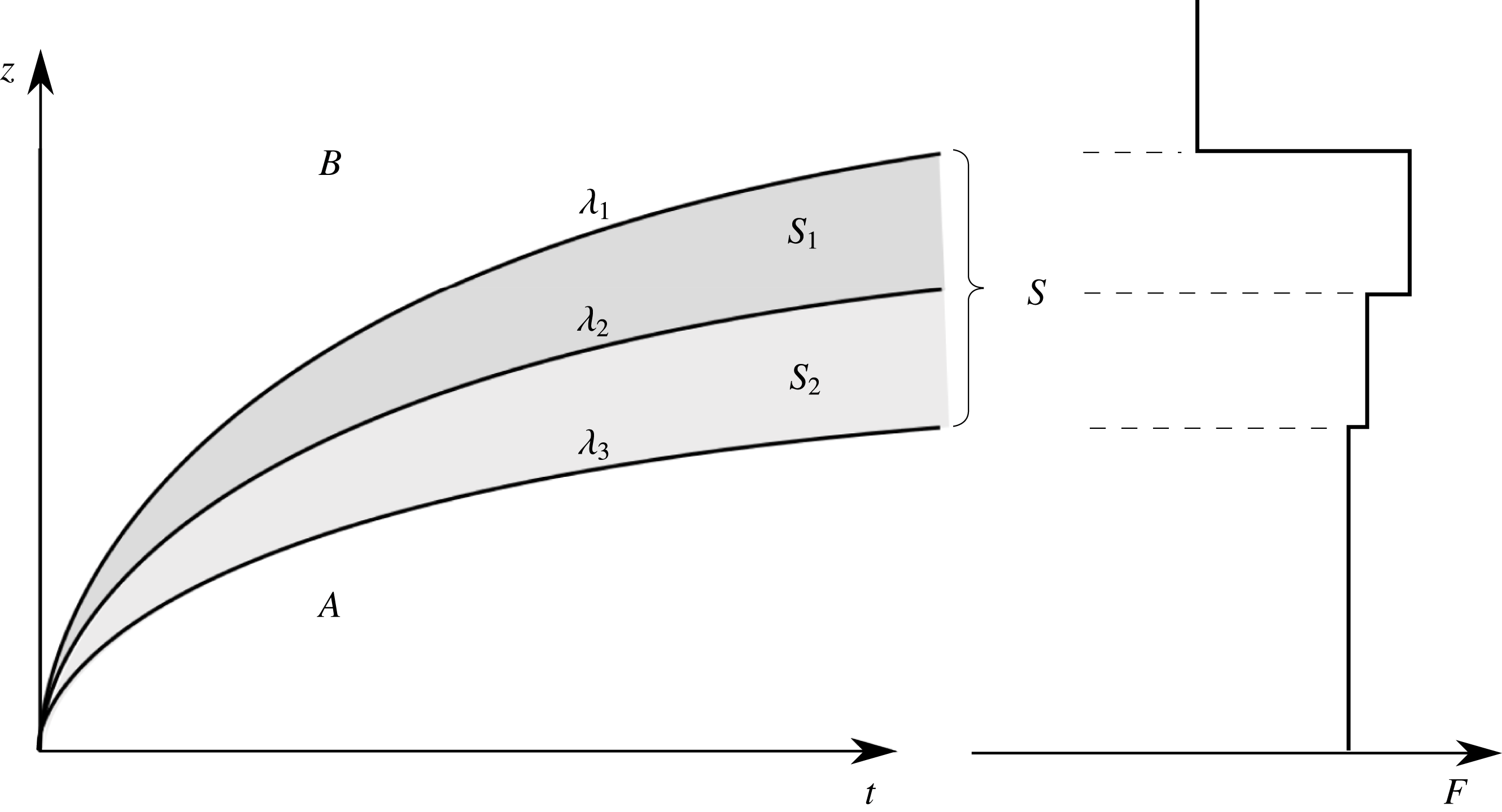
Figure 8. The three distinct characteristic curves and associated eigenvalues ${\it\lambda}_{1}$
,
${\it\lambda}_{1}$
, ${\it\lambda}_{2}$
and
${\it\lambda}_{2}$
and ${\it\lambda}_{3}$
in a generalised formulation of the unsteady plume equations. Regions
${\it\lambda}_{3}$
in a generalised formulation of the unsteady plume equations. Regions $A$
and
$A$
and $B$
denote points in
$B$
denote points in $(z,t)$
space upstream and downstream of a wave, while regions
$(z,t)$
space upstream and downstream of a wave, while regions $S_{1}$
and
$S_{1}$
and $S_{2}$
denote regions of the wave. The depicted behaviour of
$S_{2}$
denote regions of the wave. The depicted behaviour of $F$
in the wave is for schematic purposes only.
$F$
in the wave is for schematic purposes only.
The values of $M$
and
$M$
and $Q$
in the wave are not affected by the location of the second characteristic associated with
$Q$
in the wave are not affected by the location of the second characteristic associated with ${\it\lambda}_{2}$
. The buoyancy
${\it\lambda}_{2}$
. The buoyancy $B$
, however, takes distinct values in
$B$
, however, takes distinct values in $S_{1}$
and
$S_{1}$
and $S_{2}$
according to the position of the second characteristic. If it is assumed that both the source Richardson number and the source radius are fixed, we may say that
$S_{2}$
according to the position of the second characteristic. If it is assumed that both the source Richardson number and the source radius are fixed, we may say that $Q^{A}\propto F^{A\,1/3}$
,
$Q^{A}\propto F^{A\,1/3}$
, $Q^{B}\propto F^{B\,1/3}$
,
$Q^{B}\propto F^{B\,1/3}$
, $M^{A}\propto F^{A\,2/3}$
and
$M^{A}\propto F^{A\,2/3}$
and $M^{B}\propto F^{B\,2/3}$
. Hence (5.15) and (5.16) imply that
$M^{B}\propto F^{B\,2/3}$
. Hence (5.15) and (5.16) imply that
 $$\begin{eqnarray}\frac{M^{S}}{M^{A}}=\left(\frac{F^{A}}{F^{B}}\right)^{1/(6{\it\phi})-1/3},\quad \frac{Q^{S}}{Q^{A}}=\left(\frac{F^{A}}{F^{B}}\right)^{1/(6{\it\phi})-{\it\phi}/3-1/6}.\end{eqnarray}$$
Therefore, following a step change in the source buoyancy flux $F_{s}^{B}\mapsto F_{s}^{A}$
, the parameter
$F_{s}^{B}\mapsto F_{s}^{A}$
, the parameter ${\it\phi}$
, which depends on
${\it\phi}$
, which depends on ${\it\gamma}_{g}$
and
${\it\gamma}_{g}$
and ${\it\beta}_{g}$
, determines the behaviour of
${\it\beta}_{g}$
, determines the behaviour of $Q^{S}$
and
$Q^{S}$
and $M^{S}$
. In particular, for a given
$M^{S}$
. In particular, for a given $F^{A}$
and
$F^{A}$
and $F^{B}$
,
$F^{B}$
, ${\it\phi}$
will determine the step change in the plume velocity
${\it\phi}$
will determine the step change in the plume velocity $w_{m}$
in
$w_{m}$
in $S$
and therefore whether each characteristic is associated with rarefaction or compression behaviour. A rarefaction wave occurs when the characteristic velocity
$S$
and therefore whether each characteristic is associated with rarefaction or compression behaviour. A rarefaction wave occurs when the characteristic velocity $w_{m}$
undergoes a positive step change in the positive
$w_{m}$
undergoes a positive step change in the positive $z$
direction, whereas a compression wave occurs when
$z$
direction, whereas a compression wave occurs when $w_{m}$
undergoes a negative step change. For Gaussian plumes or, more generally, when
$w_{m}$
undergoes a negative step change. For Gaussian plumes or, more generally, when ${\it\gamma}_{g}/{\it\beta}_{g}=4/3$
(which implies that
${\it\gamma}_{g}/{\it\beta}_{g}=4/3$
(which implies that ${\it\phi}=1/2$
), the behaviour of the wave is particularly simple, because
${\it\phi}=1/2$
), the behaviour of the wave is particularly simple, because $Q^{S}=Q^{A}$
and
$Q^{S}=Q^{A}$
and $M^{S}=M^{A}$
. In that case the leading characteristic associated with
$M^{S}=M^{A}$
. In that case the leading characteristic associated with ${\it\lambda}_{1}$
is a rarefaction wave or a compression wave, according to whether
${\it\lambda}_{1}$
is a rarefaction wave or a compression wave, according to whether $F^{A}<F^{B}$
or
$F^{A}<F^{B}$
or $F^{A}>F^{B}$
, respectively. Furthermore, in agreement with the deductions made in the previous section, when
$F^{A}>F^{B}$
, respectively. Furthermore, in agreement with the deductions made in the previous section, when ${\it\phi}=1/2$
the plume radius
${\it\phi}=1/2$
the plume radius $r_{m}$
does not deviate from its steady-state value in the region
$r_{m}$
does not deviate from its steady-state value in the region $S$
, although, as noted previously, for this to be the case it is necessary that
$S$
, although, as noted previously, for this to be the case it is necessary that ${\it\theta}_{m}=1$
. Since these properties are inherited from unsteady jets, the reader is referred to Craske & van Reeuwijk (Reference Craske and van Reeuwijk2015b
) for further details. Here we will focus on the additional properties resulting from buoyancy, as manifest in the characteristic curve associated with
${\it\theta}_{m}=1$
. Since these properties are inherited from unsteady jets, the reader is referred to Craske & van Reeuwijk (Reference Craske and van Reeuwijk2015b
) for further details. Here we will focus on the additional properties resulting from buoyancy, as manifest in the characteristic curve associated with ${\it\lambda}_{2}$
.
${\it\lambda}_{2}$
.
Using (5.17) one can determine how the flux-balance parameter ${\it\Gamma}$
behaves in regions
${\it\Gamma}$
behaves in regions $S_{1}$
and
$S_{1}$
and $S_{2}$
:
$S_{2}$
:
 $$\begin{eqnarray}\left.\begin{array}{@{}c@{}}{\displaystyle \frac{{\it\Gamma}^{S_{1}}}{{\it\Gamma}^{B}}}=\left({\displaystyle \frac{Q^{B}}{Q^{S}}}\right)^{c_{1}-1}\left({\displaystyle \frac{M^{S}}{M^{B}}}\right)^{c_{2}-3/2}=\left({\displaystyle \frac{F^{A}}{F^{B}}}\right)^{n_{1}},\\ {\displaystyle \frac{{\it\Gamma}^{S_{2}}}{{\it\Gamma}^{A}}}=\left({\displaystyle \frac{Q^{A}}{Q^{S}}}\right)^{c_{1}-1}\left({\displaystyle \frac{M^{S}}{M^{A}}}\right)^{c_{2}-3/2}=\left({\displaystyle \frac{F^{A}}{F^{B}}}\right)^{n_{2}},\end{array}\right\}\end{eqnarray}$$
where
 $$\begin{eqnarray}n_{k}\equiv \left(c_{2}-\frac{3}{2}\right)\left(\frac{1}{6{\it\phi}}+\frac{(-1)^{k-1}}{3}\right)-(c_{1}-1)\left(\frac{1}{6{\it\phi}}-\frac{{\it\phi}}{3}+\frac{(-1)^{k-1}}{6}\right),\quad k=1,2.\quad\end{eqnarray}$$
In ${\it\Gamma}$
, unlike
${\it\Gamma}$
, unlike $Q$
and
$Q$
and $M$
, the characteristic associated with
$M$
, the characteristic associated with ${\it\lambda}_{2}$
, which is determined by the dimensionless buoyancy flux
${\it\lambda}_{2}$
, which is determined by the dimensionless buoyancy flux ${\it\theta}_{g}$
, can result in a discontinuity. In general, distinct values of
${\it\theta}_{g}$
, can result in a discontinuity. In general, distinct values of ${\it\Gamma}$
are found in regions
${\it\Gamma}$
are found in regions $S_{1}$
and
$S_{1}$
and $S_{2}$
and depend on
$S_{2}$
and depend on ${\it\gamma}_{g},{\it\beta}_{g}$
and
${\it\gamma}_{g},{\it\beta}_{g}$
and ${\it\theta}_{g}$
.
${\it\theta}_{g}$
.
When ${\it\gamma}_{g}/{\it\beta}_{g}=4/3$
the plume is straight sided,
${\it\gamma}_{g}/{\it\beta}_{g}=4/3$
the plume is straight sided, ${\it\phi}=1/2$
and
${\it\phi}=1/2$
and
 $$\begin{eqnarray}n_{1}=\frac{2c_{2}}{3}-\frac{c_{1}}{3}-\frac{2}{3},\quad n_{2}=0.\end{eqnarray}$$
Therefore, substituting for $c_{1}$
and
$c_{1}$
and $c_{2}$
using (5.11) and assuming
$c_{2}$
using (5.11) and assuming ${\it\Gamma}^{A}={\it\Gamma}^{B}=1$
,
${\it\Gamma}^{A}={\it\Gamma}^{B}=1$
,
 $$\begin{eqnarray}{\it\Gamma}^{S_{1}}\left(\frac{{\it\theta}_{g}}{{\it\gamma}_{g}}\right)=\left(\frac{F^{A}}{F^{B}}\right)^{q},\quad {\it\Gamma}^{S_{2}}({\it\theta}_{g})=1,\end{eqnarray}$$
where
 $$\begin{eqnarray}q\equiv -\frac{12({\it\theta}_{g}/{\it\gamma}_{g})^{2}-18({\it\theta}_{g}/{\it\gamma}_{g})+6}{12({\it\theta}_{g}/{\it\gamma}_{g})^{2}-24({\it\theta}_{g}/{\it\gamma}_{g})+9},\end{eqnarray}$$
such that the behaviour of ${\it\Gamma}$
over the wave depends only on the ratio of the dimensionless buoyancy flux
${\it\Gamma}$
over the wave depends only on the ratio of the dimensionless buoyancy flux ${\it\theta}_{g}$
to the dimensionless energy flux
${\it\theta}_{g}$
to the dimensionless energy flux ${\it\gamma}_{g}$
. While the plume remains pure in
${\it\gamma}_{g}$
. While the plume remains pure in $S_{2}$
(note that
$S_{2}$
(note that ${\it\Gamma}^{S_{2}}=1$
),
${\it\Gamma}^{S_{2}}=1$
), ${\it\Gamma}^{S_{1}}$
depends on the location of the second characteristic curve. If
${\it\Gamma}^{S_{1}}$
depends on the location of the second characteristic curve. If ${\it\theta}_{g}/{\it\gamma}_{g}<1$
, there is a deficit of buoyancy in
${\it\theta}_{g}/{\it\gamma}_{g}<1$
, there is a deficit of buoyancy in $S_{1}$
and the plume becomes ‘forced’ (
$S_{1}$
and the plume becomes ‘forced’ ( ${\it\Gamma}^{S1}<1$
). Conversely, if
${\it\Gamma}^{S1}<1$
). Conversely, if ${\it\theta}_{g}/{\it\gamma}_{g}>1$
surplus buoyancy enters
${\it\theta}_{g}/{\it\gamma}_{g}>1$
surplus buoyancy enters $S_{1}$
and the plume becomes ‘lazy’. These results are consistent with the condition established in § 5.2 that
$S_{1}$
and the plume becomes ‘lazy’. These results are consistent with the condition established in § 5.2 that ${\it\theta}_{g}/{\it\gamma}_{g}=1$
in order for the plume to remain pure, and are illustrated in figure 9. For details about the behaviour of
${\it\theta}_{g}/{\it\gamma}_{g}=1$
in order for the plume to remain pure, and are illustrated in figure 9. For details about the behaviour of ${\it\Gamma}$
when the fluxes in the plume are reduced according to a self-similar scaling, the reader is referred to appendix A.
${\it\Gamma}$
when the fluxes in the plume are reduced according to a self-similar scaling, the reader is referred to appendix A.
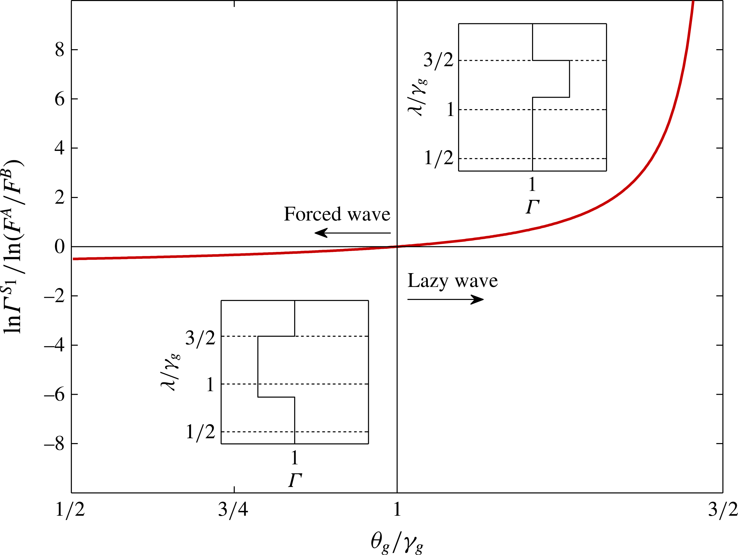
Figure 9. Wave structure in a straight-sided plume ( ${\it\gamma}_{g}/{\it\beta}_{g}=4/3$
,
${\it\gamma}_{g}/{\it\beta}_{g}=4/3$
, ${\it\theta}_{m}=1$
). The special case for which
${\it\theta}_{m}=1$
). The special case for which ${\it\Gamma}=1$
in the wave corresponds to
${\it\Gamma}=1$
in the wave corresponds to ${\it\theta}_{g}={\it\gamma}_{g}$
. The variable
${\it\theta}_{g}={\it\gamma}_{g}$
. The variable ${\it\lambda}$
is a scaled
${\it\lambda}$
is a scaled $z$
coordinate, which is defined rigorously in (6.21).
$z$
coordinate, which is defined rigorously in (6.21).
5.4 Response to source perturbations
The final property of the generalised unsteady plume equations that we consider is their response to harmonic perturbations. From a modelling perspective it is necessary to understand whether an unsteady plume model is stable with respect to source perturbations. Scase & Hewitt (Reference Scase and Hewitt2012) showed that top-hat unsteady plume models are ill posed because they admit the unbounded (exponential) growth of high-frequency source perturbations, making it impossible to obtain convergence in numerical simulations of the governing integral equations. Using the framework described in this paper, it is possible to adopt a more general approach and analyse the response of the unsteady plume equations without making an assumption about the velocity profile, turbulent transport or pressure. It is consequently possible to establish whether a given plume model is well posed. More generally, one can establish a relation between the dimensionless profile coefficients that ensures well posedness and understand how this relates to the underlying physics of an unsteady plume.
Using the dimensionless variables
 $$\begin{eqnarray}{\it\zeta}\equiv \frac{3}{4}\frac{z{\it\sigma}}{w_{m0}},\quad {\it\tau}\equiv {\it\sigma}t,\end{eqnarray}$$
with the characteristic steady-state velocity
 $$\begin{eqnarray}w_{m0}\equiv \frac{3}{4}\left(\frac{10}{9{\it\alpha}_{0}}\right)^{2/3}\left(\frac{F}{{\it\beta}_{g}{\it\theta}_{m}}\right)^{1/3}z^{-1/3},\end{eqnarray}$$
we consider a harmonic source perturbation of amplitude ${\it\epsilon}$
and seek solutions of the form
${\it\epsilon}$
and seek solutions of the form
 $$\begin{eqnarray}\left.\begin{array}{@{}c@{}}Q=Q_{0}(1+{\it\epsilon}\mathscr{Q}_{1}\ldots ),\\ M=M_{0}(1+{\it\epsilon}\mathscr{M}_{1}\ldots ),\\ B=B_{0}(1+{\it\epsilon}\mathscr{B}_{1}\ldots ).\end{array}\right\}\end{eqnarray}$$
At $O({\it\epsilon})$
the unsteady plume equations can be expressed as
$O({\it\epsilon})$
the unsteady plume equations can be expressed as
 $$\begin{eqnarray}\left(\frac{\partial }{\partial {\it\tau}}+\left[\begin{array}{@{}ccc@{}}0 & {\it\beta}_{g} & 0\\ -{\it\gamma}_{g} & 2{\it\gamma}_{g} & 0\\ -{\it\theta}_{g} & {\it\theta}_{g} & {\it\theta}_{g}\end{array}\right]\frac{\partial }{\partial {\it\zeta}}-\frac{1}{{\it\zeta}}\left[\begin{array}{@{}ccc@{}}0 & -{\it\beta}_{g} & {\it\beta}_{g}\\ \unicode[STIX]{x1D619}_{21} & \unicode[STIX]{x1D619}_{22} & \unicode[STIX]{x1D619}_{23}\\ 0 & 0 & 0\end{array}\right]\right)\left(\begin{array}{@{}c@{}}\mathscr{Q}_{1}\\ \mathscr{M}_{1}\\ \mathscr{ B}_{1}\end{array}\right)=0,\end{eqnarray}$$
where
 $$\begin{eqnarray}\unicode[STIX]{x1D619}_{21}\equiv -{\textstyle \frac{3}{4}}{\it\gamma}_{g}+2{\it\beta}_{g}{\it\theta}_{m},\quad \unicode[STIX]{x1D619}_{22}\equiv {\textstyle \frac{3}{8}}{\it\gamma}_{g}-3{\it\beta}_{g}{\it\theta}_{m},\quad \unicode[STIX]{x1D619}_{23}\equiv 2{\it\beta}_{g}{\it\theta}_{m}.\end{eqnarray}$$
In (5.27) and (5.28) we have used (2.23), rearranged as
 $$\begin{eqnarray}{\it\delta}_{g}={\it\alpha}_{0}({\textstyle \frac{6}{5}}{\it\gamma}_{g}-{\textstyle \frac{16}{5}}{\it\beta}_{g}{\it\theta}_{m}),\end{eqnarray}$$
to eliminate ${\it\delta}_{g}$
.
${\it\delta}_{g}$
.
Here we restrict our attention to a plume with velocity and buoyancy profiles of Gaussian form and equal width, and neglect the longitudinal turbulent transport of momentum. Hence, we assume that ${\it\theta}_{m}={\it\beta}_{g}=1$
and
${\it\theta}_{m}={\it\beta}_{g}=1$
and ${\it\gamma}_{g}={\it\gamma}_{m}=4/3$
and focus our attention on the way in which
${\it\gamma}_{g}={\it\gamma}_{m}=4/3$
and focus our attention on the way in which ${\it\theta}_{g}$
affects the downstream development of source perturbations, complementing the predictions pertaining to
${\it\theta}_{g}$
affects the downstream development of source perturbations, complementing the predictions pertaining to ${\it\Gamma}$
that were obtained in § 5.3. There are several reasons for focusing on straight-sided unsteady plumes at this point. First, theoretical and observational evidence suggests that if one has to choose a value of
${\it\Gamma}$
that were obtained in § 5.3. There are several reasons for focusing on straight-sided unsteady plumes at this point. First, theoretical and observational evidence suggests that if one has to choose a value of ${\it\gamma}_{m}$
, then
${\it\gamma}_{m}$
, then $4/3$
is the most appropriate choice. Second, straight sidedness is a distinguished case and therefore worthy of investigation in its own right. In the absence of compelling evidence to the contrary, we feel that it would be unhelpful and less general to restrict the parameter space in an alternative way. Third, source perturbation analysis for jets, for which straight sidedness was not assumed, was conducted in Craske & van Reeuwijk (Reference Craske and van Reeuwijk2015b
). Therefore, by focusing on the effects of buoyancy transport in the present section, we augment existing work on the subject.
$4/3$
is the most appropriate choice. Second, straight sidedness is a distinguished case and therefore worthy of investigation in its own right. In the absence of compelling evidence to the contrary, we feel that it would be unhelpful and less general to restrict the parameter space in an alternative way. Third, source perturbation analysis for jets, for which straight sidedness was not assumed, was conducted in Craske & van Reeuwijk (Reference Craske and van Reeuwijk2015b
). Therefore, by focusing on the effects of buoyancy transport in the present section, we augment existing work on the subject.
The assumed values of ${\it\beta}_{g}$
,
${\it\beta}_{g}$
, ${\it\theta}_{m}$
and
${\it\theta}_{m}$
and ${\it\gamma}_{g}$
ensure that the plume remains straight sided (see § 5.2) such that
${\it\gamma}_{g}$
ensure that the plume remains straight sided (see § 5.2) such that $\mathscr{M}_{1}=2\mathscr{Q}_{1}$
for the linearized perturbation, and thus (5.27) simplifies to
$\mathscr{M}_{1}=2\mathscr{Q}_{1}$
for the linearized perturbation, and thus (5.27) simplifies to
 $$\begin{eqnarray}\left(\frac{\partial }{\partial {\it\tau}}+\left[\begin{array}{@{}cc@{}}2 & 0\\ {\it\theta}_{g}/2 & {\it\theta}_{g}\end{array}\right]\frac{\partial }{\partial {\it\zeta}}-\frac{1}{{\it\zeta}}\left[\begin{array}{@{}cc@{}}-2 & 2\\ 0 & 0\end{array}\right]\right)\left(\begin{array}{@{}c@{}}\mathscr{M}_{1}\\ \mathscr{ B}_{1}\end{array}\right)=0.\end{eqnarray}$$
We assume an oscillatory solution of the form
 $$\begin{eqnarray}\left(\begin{array}{@{}c@{}}\mathscr{M}_{1}\\ \mathscr{ B}_{1}\end{array}\right)=\left(\begin{array}{@{}c@{}}\hat{\mathscr{M}}_{1}({\it\zeta})\\ \hat{\mathscr{B}}_{1}({\it\zeta})\end{array}\right)\exp (\text{i}\,{\it\tau}).\end{eqnarray}$$
Substitution of (5.31) into (5.30) and elimination of $\hat{\mathscr{B}}_{1}$
results in
$\hat{\mathscr{B}}_{1}$
results in
 $$\begin{eqnarray}\frac{\text{d}^{2}\hat{\mathscr{M}}_{1}}{\text{d}{\it\zeta}^{2}}+\left(\frac{5}{2{\it\zeta}}+\text{i}\left(\frac{1}{2}+\frac{1}{{\it\theta}_{g}}\right)\right)\frac{\text{d}\hat{\mathscr{M}}_{1}}{\text{d}{\it\zeta}}-\left(\frac{1}{2{\it\theta}_{g}}-\text{i}\left(\frac{1}{{\it\theta}_{g}{\it\zeta}}+\frac{1}{2{\it\zeta}}\right)\right)\hat{\mathscr{M}}_{1}=0.\end{eqnarray}$$
Transformation of the coordinate system according to ${\it\zeta}_{\ast }\equiv \text{i}({\it\theta}_{g}-2){\it\zeta}/(2{\it\theta}_{g})$
, and defining the dependent variable
${\it\zeta}_{\ast }\equiv \text{i}({\it\theta}_{g}-2){\it\zeta}/(2{\it\theta}_{g})$
, and defining the dependent variable $\hat{\mathscr{M}}_{\ast }\equiv \hat{\mathscr{M}}_{1}\exp (\text{i}{\it\zeta}/2)$
, results in
$\hat{\mathscr{M}}_{\ast }\equiv \hat{\mathscr{M}}_{1}\exp (\text{i}{\it\zeta}/2)$
, results in
 $$\begin{eqnarray}{\it\zeta}_{\ast }\frac{\text{d}^{2}\hat{\mathscr{M}}_{\ast }}{\text{d}{\it\zeta}_{\ast }^{2}}+\left(\frac{5}{2}-{\it\zeta}_{\ast }\right)\frac{\text{d}\hat{\mathscr{M}}_{\ast }}{\text{d}{\it\zeta}_{\ast }}-a\hat{\mathscr{M}}_{\ast }=0,\end{eqnarray}$$
where
 $$\begin{eqnarray}a\equiv \frac{3{\it\theta}_{g}-4}{2{\it\theta}_{g}-4}.\end{eqnarray}$$
Equation (5.33) is a confluent hypergeometric equation (Abramowitz & Stegun Reference Abramowitz and Stegun1970, § 13, p. 504), whose solution can be expressed as
 $$\begin{eqnarray}\hat{\mathscr{M}}_{1}({\it\zeta})=\left(c_{1}\text{M}\left(a,\frac{5}{2},\text{i}\frac{{\it\theta}_{g}-2}{2{\it\theta}_{g}}{\it\zeta}\right)+c_{2}\text{U}\left(a,\frac{5}{2},\text{i}\frac{{\it\theta}_{g}-2}{2{\it\theta}_{g}}{\it\zeta}\right)\right)\text{exp}\left(-\text{i}\frac{{\it\zeta}}{2}\right),\end{eqnarray}$$
where the independent solutions $\text{M}$
and
$\text{M}$
and $\text{U}$
are Kummer functions. At the source, (5.35) implies that
$\text{U}$
are Kummer functions. At the source, (5.35) implies that $\mathscr{B}_{1}(0)=\mathscr{M}_{1}(0)~\forall c_{1},c_{2}$
, which means that to leading order
$\mathscr{B}_{1}(0)=\mathscr{M}_{1}(0)~\forall c_{1},c_{2}$
, which means that to leading order ${\it\Gamma}(0)=1$
. To ensure finite
${\it\Gamma}(0)=1$
. To ensure finite $\hat{\mathscr{M}}_{1}(0)$
, we set
$\hat{\mathscr{M}}_{1}(0)$
, we set $c_{2}=0$
and assume that
$c_{2}=0$
and assume that $c_{1}=1$
, without loss of generality. The asymptotic expansion of (5.35), for
$c_{1}=1$
, without loss of generality. The asymptotic expansion of (5.35), for ${\it\zeta}\rightarrow \infty$
and
${\it\zeta}\rightarrow \infty$
and $0\leqslant {\it\theta}_{g}<2$
, is
$0\leqslant {\it\theta}_{g}<2$
, is
 $$\begin{eqnarray}\hat{\mathscr{M}}_{1}({\it\zeta})\sim \frac{3\sqrt{{\rm\pi}}}{4\unicode[STIX]{x1D758}(5/2-a)}\left(\frac{2{\it\theta}_{g}}{{\it\theta}_{g}-2}\right)^{a}\text{exp}\left(-\text{i}\frac{{\it\zeta}}{2}\right){\it\zeta}^{-a},\end{eqnarray}$$
where $\unicode[STIX]{x1D758}$
is the Gamma function. The exponent
$\unicode[STIX]{x1D758}$
is the Gamma function. The exponent $a({\it\theta}_{g})$
therefore determines the growth rate of the perturbations, as illustrated in figure 10. When
$a({\it\theta}_{g})$
therefore determines the growth rate of the perturbations, as illustrated in figure 10. When $1\leqslant {\it\theta}_{g}<4/3$
(forced waves, according to § 5.3), the growth rate is negative, but when
$1\leqslant {\it\theta}_{g}<4/3$
(forced waves, according to § 5.3), the growth rate is negative, but when $4/3<{\it\theta}_{g}<2$
(lazy waves), the growth rate is positive. Between growth and decay of source perturbations lies the special behaviour associated with
$4/3<{\it\theta}_{g}<2$
(lazy waves), the growth rate is positive. Between growth and decay of source perturbations lies the special behaviour associated with ${\it\theta}_{g}=4/3$
, for which the plume is pure and exhibits a neutral response to source perturbations. We note that
${\it\theta}_{g}=4/3$
, for which the plume is pure and exhibits a neutral response to source perturbations. We note that ${\it\theta}_{g}\equiv {\it\theta}_{m}+{\it\theta}_{f}$
is not likely to exceed
${\it\theta}_{g}\equiv {\it\theta}_{m}+{\it\theta}_{f}$
is not likely to exceed $4/3$
in practice (see e.g. table 2) because
$4/3$
in practice (see e.g. table 2) because ${\it\theta}_{m}\approx 1$
and the dimensionless turbulent buoyancy flux
${\it\theta}_{m}\approx 1$
and the dimensionless turbulent buoyancy flux ${\it\theta}_{f}\approx 0.2$
. Therefore, this analysis demonstrates that the generalised unsteady plume equations are well posed for physically realistic values of the dimensionless profile coefficients.
${\it\theta}_{f}\approx 0.2$
. Therefore, this analysis demonstrates that the generalised unsteady plume equations are well posed for physically realistic values of the dimensionless profile coefficients.
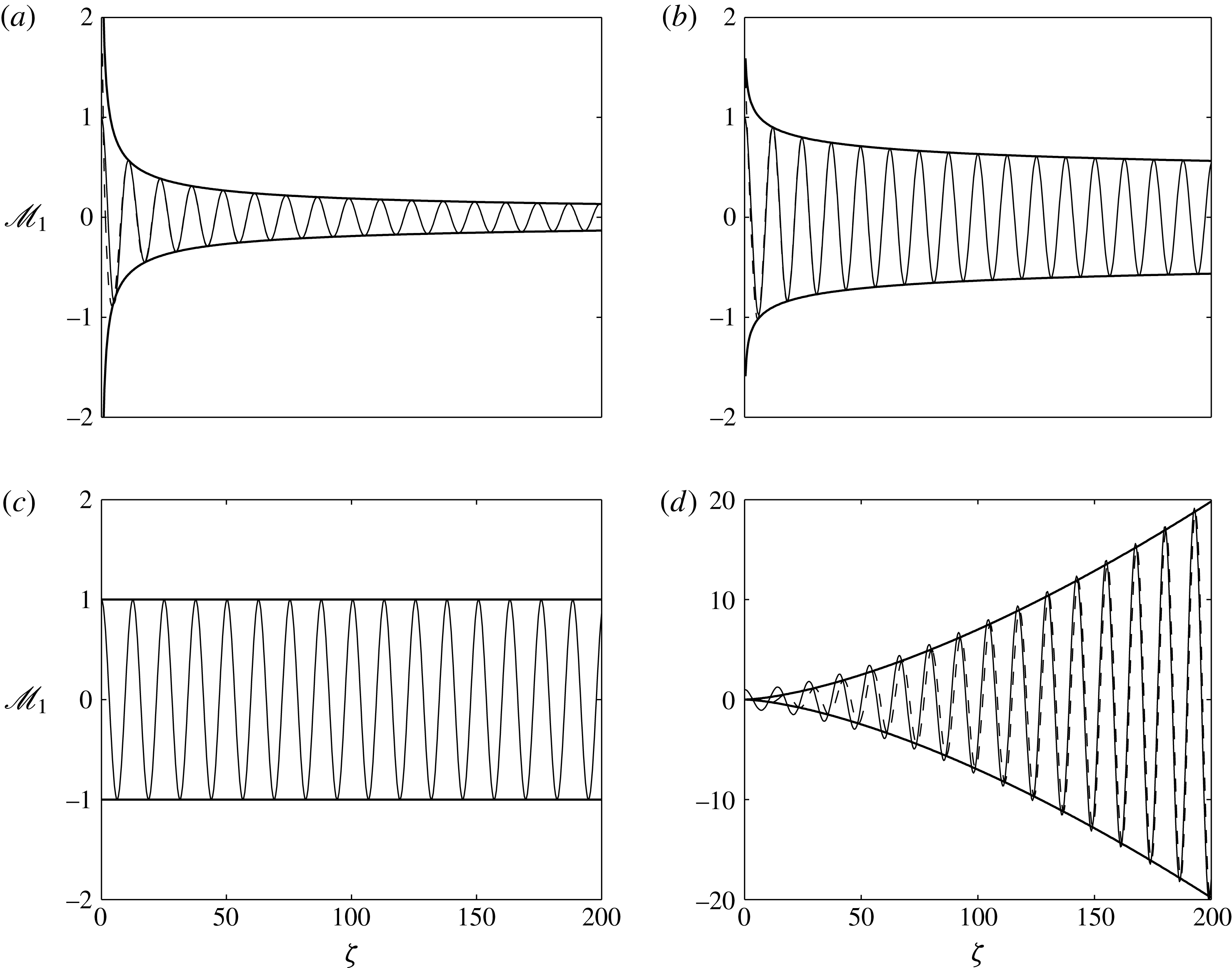
Figure 10. Stability of the system when ${\it\gamma}_{m}=4/3$
in response to source perturbations with respect to the dimensionless longitudinal coordinate
${\it\gamma}_{m}=4/3$
in response to source perturbations with respect to the dimensionless longitudinal coordinate ${\it\zeta}\propto z^{4/3}{\it\sigma}$
for (a)
${\it\zeta}\propto z^{4/3}{\it\sigma}$
for (a) ${\it\theta}_{g}=1$
; (b)
${\it\theta}_{g}=1$
; (b) ${\it\theta}_{g}=5/4$
; (c)
${\it\theta}_{g}=5/4$
; (c) ${\it\theta}_{g}=4/3$
and (d)
${\it\theta}_{g}=4/3$
and (d) ${\it\theta}_{g}=5/3$
. The thin solid lines correspond to the exact solution of the linearized problem (5.35) and the thin dashed lines to the asymptotic solution (5.36). The thick lines denote the envelope of the asymptotic solution. The dimensionless buoyancy flux
${\it\theta}_{g}=5/3$
. The thin solid lines correspond to the exact solution of the linearized problem (5.35) and the thin dashed lines to the asymptotic solution (5.36). The thick lines denote the envelope of the asymptotic solution. The dimensionless buoyancy flux ${\it\theta}_{g}=4/3$
is the special case for which perturbations exhibit neutral growth. For models employing realistic values
${\it\theta}_{g}=4/3$
is the special case for which perturbations exhibit neutral growth. For models employing realistic values ${\it\theta}_{g}\leqslant 4/3$
, the system is well posed in the sense that source perturbations are bounded and it is possible to obtain convergent numerical approximations.
${\it\theta}_{g}\leqslant 4/3$
, the system is well posed in the sense that source perturbations are bounded and it is possible to obtain convergent numerical approximations.
6 A Gaussian unsteady plume model
In this section we propose a series of progressively simpler models for unsteady plumes, derived from the generalised unsteady plume theory developed in §§ 2 and 5. The aim is to invoke assumptions about the dimensionless profile coefficients appearing in the integral equations (2.9)–(2.11) to close the system. All of the models we propose are based on the assumption that in the steady state the plume has a Gaussian velocity profile. In § 6.1 we argue that in unsteady situations the profile coefficients are not strictly constant but functions of the dependent variables, or, more precisely, their longitudinal gradients. In § 6.2 we compare the full model to the DNS results and in § 6.3 we propose a simpler form of the model by invoking additional assumptions based on the findings of § 5.
6.1 Shear-flow dispersion
In the previous section we established the response of a plume when the profile coefficients are constant. In that case the plume integrals are, in general, discontinuous along characteristic curves, as illustrated schematically in figure 8. However, it is readily apparent from figure 4 that the plume integrals are continuous, varying smoothly from their value upstream of the disturbance to their value downstream of the disturbance. The longitudinal gradients that are produced by unsteady changes in the plume are capable of inducing a local departure from self-similarity. Noting that constant profile coefficients are a necessary condition for self-similarity, one would expect the profile coefficients to deviate from their steady-state value in the vicinity of a sudden change in the plume’s integral quantities. Taylor (Reference Taylor1953) analysed an equivalent situation in pipe flow, showing that in the vicinity of a step increase in the radially averaged scalar concentration there exists a deformation in the otherwise radially uniform concentration field. In correlation with a non-uniform velocity field, the deformation results in a local increase in the scalar flux, which, to leading order, satisfies a dispersive analogue of Fick’s law. Similarly, in Craske & van Reeuwijk (Reference Craske and van Reeuwijk2015b ), a dispersion closure was developed for energy transport in jets, which we will apply here to model the higher-order transport of buoyancy and energy in unsteady plumes.
In order to focus on longitudinal changes that constitute a departure from a steady state, it is convenient to examine dimensionless quantities. For a given quantity $f_{m}(z,t)$
, we define
$f_{m}(z,t)$
, we define $\mathscr{F}\equiv f_{m}/f_{m0}$
, where
$\mathscr{F}\equiv f_{m}/f_{m0}$
, where $f_{m0}$
is the steady-state value of
$f_{m0}$
is the steady-state value of $f_{m}$
. To quantify the departure from the steady state, we can compute the longitudinal gradient of
$f_{m}$
. To quantify the departure from the steady state, we can compute the longitudinal gradient of $\mathscr{F}$
:
$\mathscr{F}$
:
 $$\begin{eqnarray}\frac{r_{m}}{\mathscr{F}}\frac{\partial \mathscr{F}}{\partial z}=\frac{r_{m}}{f_{m}}\frac{\partial f_{m}}{\partial z}-\frac{r_{m}}{f_{m0}}\frac{\partial f_{m0}}{\partial z}.\end{eqnarray}$$
Noting that $r_{m}=6{\it\alpha}_{0}z/5$
in the steady state, it is convenient to define the steady-state function
$r_{m}=6{\it\alpha}_{0}z/5$
in the steady state, it is convenient to define the steady-state function $f_{m0}$
locally:
$f_{m0}$
locally:
 $$\begin{eqnarray}\frac{\partial f_{m0}}{\partial z}=\frac{6{\it\alpha}_{0}n}{5}\frac{f_{m0}}{r_{m}},\end{eqnarray}$$
where $f_{m0}\propto z^{n}$
, which means that the second term on the right-hand side of (6.1) is equal to
$f_{m0}\propto z^{n}$
, which means that the second term on the right-hand side of (6.1) is equal to $-6{\it\alpha}_{0}n/5$
. This is a sensible choice in general, because it means that departures from a steady state are defined relative to the local (in
$-6{\it\alpha}_{0}n/5$
. This is a sensible choice in general, because it means that departures from a steady state are defined relative to the local (in $z$
) size of the plume rather than the size it should have with respect to a fixed virtual source. Of course, if the plume is straight sided, such that
$z$
) size of the plume rather than the size it should have with respect to a fixed virtual source. Of course, if the plume is straight sided, such that $r_{m}\propto z~\forall t$
, the definitions coincide. In particular, we define the dimensionless velocity and buoyancy:
$r_{m}\propto z~\forall t$
, the definitions coincide. In particular, we define the dimensionless velocity and buoyancy:
 $$\begin{eqnarray}\mathscr{U}\equiv \frac{w_{m}}{w_{m0}},\quad \mathscr{B}\equiv \frac{b_{m}}{b_{m0}},\end{eqnarray}$$
where $w_{m0}\propto z^{-1/3}$
and
$w_{m0}\propto z^{-1/3}$
and $b_{m0}\propto z^{-5/3}$
are the steady-state power-law solutions for the velocity and buoyancy respectively. Using (6.1), with
$b_{m0}\propto z^{-5/3}$
are the steady-state power-law solutions for the velocity and buoyancy respectively. Using (6.1), with $\mathscr{F}$
replaced with either
$\mathscr{F}$
replaced with either $\mathscr{U}$
or
$\mathscr{U}$
or $\mathscr{B}$
, we follow Craske & van Reeuwijk (Reference Craske and van Reeuwijk2015b
) and propose a closure for the dimensionless energy flux
$\mathscr{B}$
, we follow Craske & van Reeuwijk (Reference Craske and van Reeuwijk2015b
) and propose a closure for the dimensionless energy flux ${\it\gamma}_{m}$
and the dimensionless buoyancy flux
${\it\gamma}_{m}$
and the dimensionless buoyancy flux ${\it\theta}_{m}$
:
${\it\theta}_{m}$
:
 $$\begin{eqnarray}\displaystyle & \displaystyle {\it\gamma}_{m}={\it\gamma}_{0}-\frac{5}{{\it\alpha}_{0}}\frac{r_{m}}{\mathscr{U}}\frac{\partial \mathscr{U}}{\partial z}{\it\gamma}_{1}={\it\gamma}_{0}-6\left(\frac{1}{3}+\frac{5Q^{2}}{6{\it\alpha}_{0}M^{3/2}}\frac{\partial }{\partial z}\left(\frac{M}{Q}\right)\right){\it\gamma}_{1}, & \displaystyle\end{eqnarray}$$
 $$\begin{eqnarray}\displaystyle & \displaystyle {\it\theta}_{m}={\it\theta}_{0}-\frac{5}{{\it\alpha}_{0}}\frac{r_{m}}{\mathscr{B}}\frac{\partial \mathscr{B}}{\partial z}{\it\theta}_{1}={\it\theta}_{0}-6\left(\frac{5}{3}+\frac{5Q^{3}}{6{\it\alpha}_{0}M^{3/2}B}\frac{\partial }{\partial z}\left(\frac{MB}{Q^{2}}\right)\right){\it\theta}_{1}. & \displaystyle\end{eqnarray}$$
Note that the fractions $1/3$
and
$1/3$
and $5/3$
in (6.4) and (6.5), respectively, result from the fact that
$5/3$
in (6.4) and (6.5), respectively, result from the fact that $w_{m0}\sim z^{-1/3}$
and
$w_{m0}\sim z^{-1/3}$
and $b_{m0}\sim z^{-5/3}$
, respectively. Although the terms inside the parenthesis in the definition of
$b_{m0}\sim z^{-5/3}$
, respectively. Although the terms inside the parenthesis in the definition of ${\it\gamma}_{m}$
appear to differ from those presented in Craske & van Reeuwijk (Reference Craske and van Reeuwijk2015b
), the difference is superficial, as
${\it\gamma}_{m}$
appear to differ from those presented in Craske & van Reeuwijk (Reference Craske and van Reeuwijk2015b
), the difference is superficial, as ${\it\gamma}_{1}$
can be redefined to render the expressions equivalent. A notable virtue of the dispersion closure is that the incorporation of (6.5) does not affect the steady-state solutions. In contrast, the diffusive mixing term for momentum proposed by Scase & Hewitt (Reference Scase and Hewitt2012) was not extended to buoyancy transport, because it would have modified the exponents associated with the steady-state solutions.
${\it\gamma}_{1}$
can be redefined to render the expressions equivalent. A notable virtue of the dispersion closure is that the incorporation of (6.5) does not affect the steady-state solutions. In contrast, the diffusive mixing term for momentum proposed by Scase & Hewitt (Reference Scase and Hewitt2012) was not extended to buoyancy transport, because it would have modified the exponents associated with the steady-state solutions.
6.2 Unsteady plume model
For the purposes of establishing a relatively simple representation of an unsteady plume, we neglect turbulent transport and assume ${\it\gamma}_{g}={\it\gamma}_{m}$
,
${\it\gamma}_{g}={\it\gamma}_{m}$
, ${\it\theta}_{g}={\it\theta}_{m}$
and
${\it\theta}_{g}={\it\theta}_{m}$
and ${\it\beta}_{g}={\it\beta}_{m}$
, resulting in the following model
${\it\beta}_{g}={\it\beta}_{m}$
, resulting in the following model
 $$\begin{eqnarray}\displaystyle & \displaystyle \frac{\partial Q}{\partial t}+\frac{\partial M}{\partial z}=B, & \displaystyle\end{eqnarray}$$
 $$\begin{eqnarray}\displaystyle & \displaystyle \frac{\partial M}{\partial t}+{\it\gamma}_{0}\frac{\partial }{\partial z}\left(\frac{M^{2}}{Q}\right)={\it\delta}_{m}\frac{M^{5/2}}{Q^{2}}+\frac{5{\it\gamma}_{1}}{{\it\alpha}_{0}}\frac{\partial }{\partial z}\left(\frac{M^{3/2}}{\mathscr{U}}\frac{\partial \mathscr{U}}{\partial z}\right)+2{\it\theta}_{m}\frac{MB}{Q}, & \displaystyle\end{eqnarray}$$
 $$\begin{eqnarray}\displaystyle & \displaystyle \frac{\partial B}{\partial t}+{\it\theta}_{0}\frac{\partial }{\partial z}\left(\frac{MB}{Q}\right)=\frac{5{\it\theta}_{1}}{{\it\alpha}_{0}}\frac{\partial }{\partial z}\left(\frac{M^{1/2}B}{\mathscr{B}}\frac{\partial \mathscr{B}}{\partial z}\right). & \displaystyle\end{eqnarray}$$
In the interest of brevity, ${\it\theta}_{m}$
on the right-hand side of (6.7) has not been expanded and for consistency should therefore be replaced with (6.5).
${\it\theta}_{m}$
on the right-hand side of (6.7) has not been expanded and for consistency should therefore be replaced with (6.5).
We solve the system (6.6)–(6.8) using fourth-order accurate central differences and a fourth-order Runge–Kutta method for integration with respect to $t$
. To adequately describe both near- and far-field scales in the plume we employ a stretched computational grid in space, for which the ratio of the first and last computational cells is approximately equal to 0.1. At the first and last computational cells the values of the dependent variables are held constant (i.e. independent of time), and by letting the height of the domain be equal to
$t$
. To adequately describe both near- and far-field scales in the plume we employ a stretched computational grid in space, for which the ratio of the first and last computational cells is approximately equal to 0.1. At the first and last computational cells the values of the dependent variables are held constant (i.e. independent of time), and by letting the height of the domain be equal to $64r_{s}$
we ensure that the outflow condition has a negligible influence in those parts of the domain with which we are primarily concerned. As indicated in figure 4(a,c,e), smooth initial conditions for
$64r_{s}$
we ensure that the outflow condition has a negligible influence in those parts of the domain with which we are primarily concerned. As indicated in figure 4(a,c,e), smooth initial conditions for $Q,M$
and
$Q,M$
and $B$
were obtained by fitting an error function to the observed buoyancy flux
$B$
were obtained by fitting an error function to the observed buoyancy flux $F$
at
$F$
at $t=t_{1}$
and by substituting
$t=t_{1}$
and by substituting $F(z,t_{1})$
into the steady-state solutions (2.22). Although this method of determining initial conditions is approximate, at
$F(z,t_{1})$
into the steady-state solutions (2.22). Although this method of determining initial conditions is approximate, at $t=t_{1}$
the unsteady part of the flow is very close to the source and a precise description of the rapid change in
$t=t_{1}$
the unsteady part of the flow is very close to the source and a precise description of the rapid change in $F$
from
$F$
from $F^{B}$
to
$F^{B}$
to $F^{A}$
makes little difference to predictions at later times. For
$F^{A}$
makes little difference to predictions at later times. For $t>t_{1}$
,
$t>t_{1}$
, $Q,M$
and
$Q,M$
and $B$
are held constant at the source.
$B$
are held constant at the source.
We compare our model’s predictions, which we refer to as the Gaussian plume model (GPM), to those of the adjusted top-hat plume model (TPM) proposed by Scase & Hewitt (Reference Scase and Hewitt2012). For the parameters of GPM we assume Gaussian profiles and neglect turbulence transport, setting ${\it\gamma}_{0}=4/3$
and
${\it\gamma}_{0}=4/3$
and ${\it\theta}_{0}=1$
. For the higher-order mixing terms we use
${\it\theta}_{0}=1$
. For the higher-order mixing terms we use ${\it\gamma}_{1}={\it\theta}_{1}=0.0017$
. For the parameter
${\it\gamma}_{1}={\it\theta}_{1}=0.0017$
. For the parameter ${\it\varepsilon}$
that appears in the regularisation proposed by Scase & Hewitt (Reference Scase and Hewitt2012) we set
${\it\varepsilon}$
that appears in the regularisation proposed by Scase & Hewitt (Reference Scase and Hewitt2012) we set ${\it\varepsilon}=5{\it\gamma}_{1}$
, which ensures that the diffusive flux of energy in TPM is equal to the dispersive flux of energy in GPM (see Craske & van Reeuwijk Reference Craske and van Reeuwijk2015b
). To obtain predictions from TPM it was necessary to employ a flux-limiting scheme, and to this end we followed Kurganov & Tadmor (Reference Kurganov and Tadmor2000). For TPM it was also necessary to use 4000 computational points to obtain a converged prediction, which was verified by halving the number of points to 2000. In contrast, a converged prediction was obtained from GPM using only 400 computational points, and therefore took significantly less time to compute than TPM.
${\it\varepsilon}=5{\it\gamma}_{1}$
, which ensures that the diffusive flux of energy in TPM is equal to the dispersive flux of energy in GPM (see Craske & van Reeuwijk Reference Craske and van Reeuwijk2015b
). To obtain predictions from TPM it was necessary to employ a flux-limiting scheme, and to this end we followed Kurganov & Tadmor (Reference Kurganov and Tadmor2000). For TPM it was also necessary to use 4000 computational points to obtain a converged prediction, which was verified by halving the number of points to 2000. In contrast, a converged prediction was obtained from GPM using only 400 computational points, and therefore took significantly less time to compute than TPM.
Figures 4 and 7 compare the predictions of (6.6)–(6.8) to those of the regularised top-hat model described by Scase & Hewitt (Reference Scase and Hewitt2012). The predictions of $Q$
and
$Q$
and $M$
using GPM displayed in figure 4 are in reasonably good agreement with the DNS data. In particular, GPM correctly represents the position and the spreading rate of the wave front in
$M$
using GPM displayed in figure 4 are in reasonably good agreement with the DNS data. In particular, GPM correctly represents the position and the spreading rate of the wave front in $M$
. In the volume flux
$M$
. In the volume flux $Q$
it appears that GPM predicts that the wave front travels slightly faster than the DNS observations suggest. Nevertheless, despite using an order of magnitude fewer computational points, GPM provides a better overall agreement with the DNS observations than TPM, which predicts a large overshoot in
$Q$
it appears that GPM predicts that the wave front travels slightly faster than the DNS observations suggest. Nevertheless, despite using an order of magnitude fewer computational points, GPM provides a better overall agreement with the DNS observations than TPM, which predicts a large overshoot in $Q,M$
and
$Q,M$
and $B$
.
$B$
.
In figure 7 the predictions from GPM exhibit a good agreement with both the radius of the plume and the flux-balance parameter. TPM predicts a local increase in both $r_{m}$
and
$r_{m}$
and ${\it\Gamma}$
, which we do not observe in the DNS simulations. Consistent with the analysis of the hyperbolic problem in § 5.1, for
${\it\Gamma}$
, which we do not observe in the DNS simulations. Consistent with the analysis of the hyperbolic problem in § 5.1, for ${\it\theta}_{g}<4/3$
, GPM predicts a small reduction in
${\it\theta}_{g}<4/3$
, GPM predicts a small reduction in ${\it\Gamma}$
in the vicinity of the wave. Due to statistical uncertainty, it is not possible to say whether this prediction of a very small reduction in
${\it\Gamma}$
in the vicinity of the wave. Due to statistical uncertainty, it is not possible to say whether this prediction of a very small reduction in ${\it\Gamma}$
agrees with the DNS observations, which to leading order suggest that
${\it\Gamma}$
agrees with the DNS observations, which to leading order suggest that ${\it\Gamma}$
is approximately constant.
${\it\Gamma}$
is approximately constant.
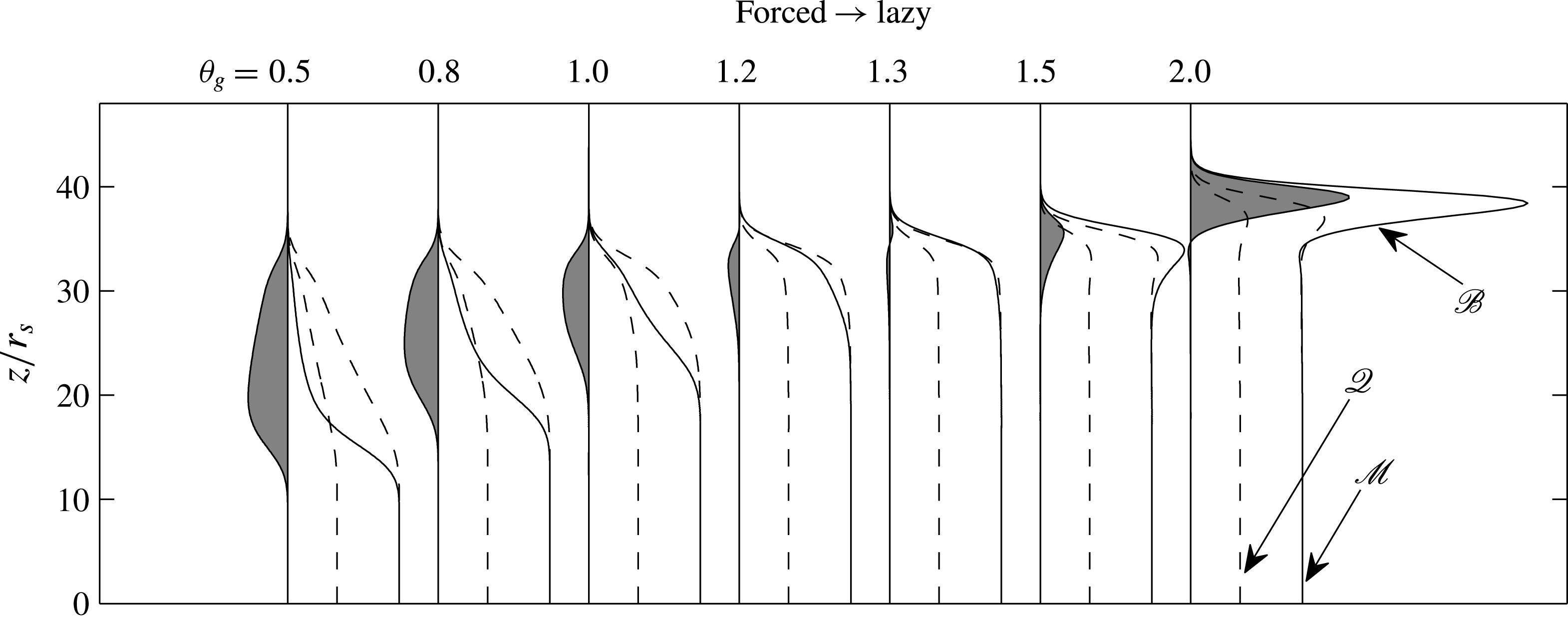
Figure 11. Wave structure for different values of ${\it\theta}_{g}$
. The dashed lines are normalised integral quantities
${\it\theta}_{g}$
. The dashed lines are normalised integral quantities $\mathscr{Q}\equiv Q/Q_{0}$
,
$\mathscr{Q}\equiv Q/Q_{0}$
, $\mathscr{M}\equiv M/M_{0}$
and the solid line is
$\mathscr{M}\equiv M/M_{0}$
and the solid line is $\mathscr{B}\equiv B/B_{0}$
. The shaded region denotes the extent to which
$\mathscr{B}\equiv B/B_{0}$
. The shaded region denotes the extent to which ${\it\Gamma}(z,t)$
is different from unity. For
${\it\Gamma}(z,t)$
is different from unity. For ${\it\theta}_{g}\approx 4/3$
,
${\it\theta}_{g}\approx 4/3$
, ${\it\Gamma}=1$
and the wave is pure.
${\it\Gamma}=1$
and the wave is pure.
There is a noticeable difference between the GPM predictions and the DNS observations of the integral buoyancy $B$
in the vicinity of the wave front (see figure 4(f)). The observations suggest that the propagating front in
$B$
in the vicinity of the wave front (see figure 4(f)). The observations suggest that the propagating front in $B$
is steeper and faster than that which is predicted by GPM. While the purpose of this paper is not to investigate the fine tuning of the various profile coefficients to give an optimised agreement with the DNS data, for physical insight and to relate our observations to the theory discussed in § 5.3, it is useful to understand the way in which unsteady plume models depend on the assumed amount of turbulent buoyancy flux. Figure 11 displays the quantities
$B$
is steeper and faster than that which is predicted by GPM. While the purpose of this paper is not to investigate the fine tuning of the various profile coefficients to give an optimised agreement with the DNS data, for physical insight and to relate our observations to the theory discussed in § 5.3, it is useful to understand the way in which unsteady plume models depend on the assumed amount of turbulent buoyancy flux. Figure 11 displays the quantities $Q(z,t)$
,
$Q(z,t)$
, $M(z,t)$
and
$M(z,t)$
and $B(z,t)$
normalised by the scalings associated with the steady state, namely
$B(z,t)$
normalised by the scalings associated with the steady state, namely $Q_{0}(z)\sim z^{5/3}$
,
$Q_{0}(z)\sim z^{5/3}$
, $M_{0}(z)\sim z^{4/3}$
and
$M_{0}(z)\sim z^{4/3}$
and $B_{0}(z)\sim z^{1/3}$
, at a fixed time. In addition, the shaded region in figure 11 indicates the extent to which the flux-balance parameter
$B_{0}(z)\sim z^{1/3}$
, at a fixed time. In addition, the shaded region in figure 11 indicates the extent to which the flux-balance parameter ${\it\Gamma}$
(2.25) deviates from unity. Each of the predictions displayed in figure 11 corresponds to a different choice of the dimensionless parameter
${\it\Gamma}$
(2.25) deviates from unity. Each of the predictions displayed in figure 11 corresponds to a different choice of the dimensionless parameter ${\it\theta}_{g}\sim {\it\theta}_{0}+{\it\theta}_{f}$
, and therefore, since
${\it\theta}_{g}\sim {\it\theta}_{0}+{\it\theta}_{f}$
, and therefore, since ${\it\theta}_{0}=0$
is fixed, to a different amount of turbulent buoyancy transport
${\it\theta}_{0}=0$
is fixed, to a different amount of turbulent buoyancy transport ${\it\theta}_{f}$
in the plume. More precisely, we add a constant
${\it\theta}_{f}$
in the plume. More precisely, we add a constant ${\it\theta}_{f}\in [0.5,2.0]$
to
${\it\theta}_{f}\in [0.5,2.0]$
to ${\it\theta}_{0}$
in (6.8) to account for the turbulent transport of buoyancy. Values of
${\it\theta}_{0}$
in (6.8) to account for the turbulent transport of buoyancy. Values of ${\it\theta}_{g}$
much less or greater than unity, although physically unrealistic, have been included in figure 11 to provide a more complete picture of the system’s response.
${\it\theta}_{g}$
much less or greater than unity, although physically unrealistic, have been included in figure 11 to provide a more complete picture of the system’s response.
The wave in the dimensionless buoyancy integral $\mathscr{B}$
in figure 11 appears to propagate faster for large values of
$\mathscr{B}$
in figure 11 appears to propagate faster for large values of ${\it\theta}_{g}$
than for small values of
${\it\theta}_{g}$
than for small values of ${\it\theta}_{g}$
, due to the distribution of buoyancy within the wave. In agreement with the analysis of § 5.3, it is also clear that the wave is lazy when
${\it\theta}_{g}$
, due to the distribution of buoyancy within the wave. In agreement with the analysis of § 5.3, it is also clear that the wave is lazy when ${\it\theta}_{g}>4/3$
and forced when
${\it\theta}_{g}>4/3$
and forced when ${\it\theta}_{g}<4/3$
. As
${\it\theta}_{g}<4/3$
. As ${\it\theta}_{g}$
increases, one observes that the front in the integral buoyancy
${\it\theta}_{g}$
increases, one observes that the front in the integral buoyancy $B$
becomes steeper, in spite of the fact that the longitudinal mixing (dispersion) parameter
$B$
becomes steeper, in spite of the fact that the longitudinal mixing (dispersion) parameter ${\it\theta}_{1}$
is identical in each case. Hence, the reason for the disparity between the GPM prediction of
${\it\theta}_{1}$
is identical in each case. Hence, the reason for the disparity between the GPM prediction of $B$
and the DNS results in figure 4 is not the higher-order term on the right-hand side of (6.8), but that by setting
$B$
and the DNS results in figure 4 is not the higher-order term on the right-hand side of (6.8), but that by setting ${\it\theta}_{0}=1$
we neglected the turbulent buoyancy flux. As indicated in figure 11, when the turbulent transport of buoyancy is included (e.g.
${\it\theta}_{0}=1$
we neglected the turbulent buoyancy flux. As indicated in figure 11, when the turbulent transport of buoyancy is included (e.g. ${\it\theta}_{g}\sim {\it\theta}_{0}=1.2$
), the wave front in
${\it\theta}_{g}\sim {\it\theta}_{0}=1.2$
), the wave front in $B$
predicted by GPM becomes steeper and exhibits a better agreement with the features of
$B$
predicted by GPM becomes steeper and exhibits a better agreement with the features of $B$
observed in figure 4.
$B$
observed in figure 4.
6.3 Pure straight-sided unsteady plume model
Motivated by the observations reported in § 4 and the theory developed in § 5, the model we derive in this section is based on two main assumptions; (1) the plume is straight sided $(r_{m}=6{\it\alpha}_{0}z/5~\forall t)$
, hence
$(r_{m}=6{\it\alpha}_{0}z/5~\forall t)$
, hence ${\it\gamma}_{g}/{\it\beta}_{g}=4/3$
and
${\it\gamma}_{g}/{\it\beta}_{g}=4/3$
and ${\it\theta}_{m}=1$
(see § 5.2); (2) the plume remains pure
${\it\theta}_{m}=1$
(see § 5.2); (2) the plume remains pure $({\it\Gamma}=1~\forall t)$
, hence
$({\it\Gamma}=1~\forall t)$
, hence ${\it\theta}_{g}={\it\gamma}_{g}$
(see § 5.2). For definiteness, we will neglect the turbulent transport of momentum and set
${\it\theta}_{g}={\it\gamma}_{g}$
(see § 5.2). For definiteness, we will neglect the turbulent transport of momentum and set ${\it\beta}_{g}=1$
, which implies that
${\it\beta}_{g}=1$
, which implies that ${\it\gamma}_{g}=4/3$
. Under these conditions the structure of the wave described in § 5.3 is particularly simple because it consists of a single front propagating along the fastest characteristic curve. Behind the front the plume behaves in accordance with a steady state. Noting from (5.4) that when
${\it\gamma}_{g}=4/3$
. Under these conditions the structure of the wave described in § 5.3 is particularly simple because it consists of a single front propagating along the fastest characteristic curve. Behind the front the plume behaves in accordance with a steady state. Noting from (5.4) that when ${\it\gamma}_{g}=4/3$
and
${\it\gamma}_{g}=4/3$
and ${\it\beta}_{g}=1$
the dimensionless velocity of the fastest characteristic is
${\it\beta}_{g}=1$
the dimensionless velocity of the fastest characteristic is ${\it\lambda}^{\ast }={\it\lambda}_{1}=3{\it\gamma}_{g}/2$
, we find that
${\it\lambda}^{\ast }={\it\lambda}_{1}=3{\it\gamma}_{g}/2$
, we find that ${\it\theta}_{g}={\it\gamma}_{g}=2{\it\lambda}^{\ast }/3$
for consistency.
${\it\theta}_{g}={\it\gamma}_{g}=2{\it\lambda}^{\ast }/3$
for consistency.
In the light of our observations from steady plumes (see table 2), the validity of assuming that ${\it\theta}_{g}={\it\gamma}_{g}$
is questionable. Thus, for situations in which the prediction of changes in
${\it\theta}_{g}={\it\gamma}_{g}$
is questionable. Thus, for situations in which the prediction of changes in ${\it\Gamma}$
in an unsteady plume are crucial, we recommend use of the full Gaussian model described in § 6.1. However, the model we describe below is valuable in its own right as a simple analytical means of obtaining a first approximation to the behaviour of an unsteady plume and for providing physical intuition. It is also of theoretical value as a distinguished case, illustrating that under the aforementioned assumptions the behaviour of an unsteady plume is similar to that of an unsteady jet (cf. Craske & van Reeuwijk Reference Craske and van Reeuwijk2015b
).
${\it\Gamma}$
in an unsteady plume are crucial, we recommend use of the full Gaussian model described in § 6.1. However, the model we describe below is valuable in its own right as a simple analytical means of obtaining a first approximation to the behaviour of an unsteady plume and for providing physical intuition. It is also of theoretical value as a distinguished case, illustrating that under the aforementioned assumptions the behaviour of an unsteady plume is similar to that of an unsteady jet (cf. Craske & van Reeuwijk Reference Craske and van Reeuwijk2015b
).
We start by considering the transport equation for buoyancy:
 $$\begin{eqnarray}\frac{\partial B}{\partial t}+\frac{\partial }{\partial z}\left({\it\theta}_{g}\frac{MB}{Q}\right)=0.\end{eqnarray}$$
Since we are assuming that the plume remains pure and straight sided,
 $$\begin{eqnarray}\frac{Q}{M^{1/2}}=\frac{6{\it\alpha}_{0}}{5}z,\quad \frac{M^{3/2}}{Q}=\frac{5B}{8{\it\alpha}_{0}},\end{eqnarray}$$
hence
 $$\begin{eqnarray}\frac{M}{Q}=\left(\frac{25}{48{\it\alpha}_{0}^{2}}\frac{B}{z}\right)^{1/2},\end{eqnarray}$$
and thus
 $$\begin{eqnarray}\frac{\partial B}{\partial t}+\frac{5\sqrt{3}}{12{\it\alpha}_{0}}\frac{\partial }{\partial z}\left(\frac{{\it\theta}_{g}B^{3/2}}{z^{1/2}}\right)=0.\end{eqnarray}$$
To include longitudinal spreading of the wave due to dispersion, we employ (6.5), which in this case reduces to
 $$\begin{eqnarray}{\it\theta}_{g}=\underbrace{{\it\theta}_{0}}_{2{\it\lambda}^{\ast }/3}-6{\it\theta}_{1}\left(\frac{5}{3}+\frac{z^{3}}{B}\frac{\partial }{\partial z}\left(\frac{B}{z^{2}}\right)\right).\end{eqnarray}$$
Note that ${\it\theta}_{1}\ll {\it\theta}_{0}$
, implying that, for smoothly varying
${\it\theta}_{1}\ll {\it\theta}_{0}$
, implying that, for smoothly varying $B$
, the effect of
$B$
, the effect of ${\it\theta}_{1}$
on
${\it\theta}_{1}$
on ${\it\theta}_{g}$
is extremely small and therefore does not significantly violate our assumption that
${\it\theta}_{g}$
is extremely small and therefore does not significantly violate our assumption that ${\it\theta}_{g}=2{\it\lambda}^{\ast }/3$
, which is required for pure-plume behaviour. The transport equation for the buoyancy integral becomes
${\it\theta}_{g}=2{\it\lambda}^{\ast }/3$
, which is required for pure-plume behaviour. The transport equation for the buoyancy integral becomes
 $$\begin{eqnarray}\frac{\partial B}{\partial t}+\frac{5\sqrt{3}{\it\lambda}^{\ast }}{18{\it\alpha}_{0}}\frac{\partial }{\partial z}\left(\frac{B^{3/2}}{z^{1/2}}\right)=\frac{5\sqrt{3}{\it\theta}_{1}}{6{\it\alpha}_{0}}\frac{\partial }{\partial z}\left(\frac{3B^{3/2}}{z^{1/2}}+2z^{5/2}\frac{\partial }{\partial z}\left(\frac{B^{3/2}}{z^{2}}\right)\right).\end{eqnarray}$$
For a given solution of (6.14) one can derive the volume flux and momentum flux by inverting (6.10):
 $$\begin{eqnarray}Q=\frac{3{\it\alpha}_{0}}{5}\sqrt{3Bz^{3}},\quad M=\frac{3}{4}Bz.\end{eqnarray}$$
In order to use (6.14) in practice, one needs to specify the dispersion parameter ${\it\theta}_{1}$
, in addition to the steady-state entrainment coefficient
${\it\theta}_{1}$
, in addition to the steady-state entrainment coefficient ${\it\alpha}_{0}$
. The remaining parameter
${\it\alpha}_{0}$
. The remaining parameter ${\it\lambda}^{\ast }=3{\it\gamma}_{g}/2=2$
is determined from the assumption that
${\it\lambda}^{\ast }=3{\it\gamma}_{g}/2=2$
is determined from the assumption that ${\it\gamma}_{g}=4/3$
.
${\it\gamma}_{g}=4/3$
.
6.4 Linearized similarity solution
Guided by the observations of § 4.2 (in particular, see figure 5), one expects unsteady disturbances in a plume to evolve in self-similar fashion sufficiently far from the source; hence we seek a similarity solution to (6.14). To simplify the analysis we will assume that the imposed change in the buoyancy flux is relatively small and consider a perturbation expansion for $B$
, where the small parameter
$B$
, where the small parameter ${\it\epsilon}$
depends on the magnitude of the imposed step change in the source buoyancy flux:
${\it\epsilon}$
depends on the magnitude of the imposed step change in the source buoyancy flux:
 $$\begin{eqnarray}B=B^{\ast }(1+{\it\epsilon}\mathscr{B}_{1}+{\it\epsilon}^{2}\mathscr{B}_{2}+\cdots \,),\end{eqnarray}$$
where
 $$\begin{eqnarray}B^{\ast }=\frac{6{\it\alpha}_{0}}{5}\left(\frac{10}{9{\it\alpha}_{0}}\right)^{1/3}z^{1/3}F^{\ast \,2/3},\end{eqnarray}$$
and $F^{\ast }$
was defined in (4.4). To first order, the conditions of straight sidedness and constant
$F^{\ast }$
was defined in (4.4). To first order, the conditions of straight sidedness and constant ${\it\Gamma}$
can be expressed as
${\it\Gamma}$
can be expressed as
 $$\begin{eqnarray}\mathscr{M}_{1}=\mathscr{B}_{1},\quad \mathscr{Q}_{1}=\mathscr{B}_{1}/2.\end{eqnarray}$$
At $O({\it\epsilon})$
we find that
$O({\it\epsilon})$
we find that
 $$\begin{eqnarray}\frac{\partial \mathscr{B}_{1}}{\partial t}+\frac{3}{4}\left({\it\lambda}^{\ast }-6{\it\theta}_{1}\right)\left(\frac{10}{9{\it\alpha}_{0}}\right)^{2/3}\left(\frac{F^{\ast }}{z}\right)^{1/3}\frac{\partial \mathscr{B}_{1}}{\partial z}=\frac{9{\it\theta}_{1}}{2}\left(\frac{10}{9{\it\alpha}_{0}}\right)^{2/3}\left(F^{\ast }z^{2}\right)^{1/3}\frac{\partial ^{2}\mathscr{B}_{1}}{\partial z^{2}}.\end{eqnarray}$$
Recalling that
 $$\begin{eqnarray}\frac{\text{d}z^{\ast }}{\text{d}t}=\frac{3{\it\lambda}^{\ast }}{4}\left(\frac{10}{9{\it\alpha}_{0}}\right)^{2/3}\frac{F^{\ast \,1/3}}{z^{\ast \,1/3}},\end{eqnarray}$$
along the leading characteristic curves of the original hyperbolic system, it is natural to define a similarity variable
 $$\begin{eqnarray}{\it\lambda}\equiv \left(\frac{9{\it\alpha}_{0}}{10}\right)^{2/3}\frac{z^{4/3}}{F^{\ast \,1/3}t},\end{eqnarray}$$

Figure 12. Predictions using a linearized, straight-sided, constant- ${\it\Gamma}$
model, for which
${\it\Gamma}$
model, for which ${\it\lambda}^{\ast }=2$
. The circles denote the prediction that is obtained by solving (6.22) numerically and the solid black line denotes the solution for
${\it\lambda}^{\ast }=2$
. The circles denote the prediction that is obtained by solving (6.22) numerically and the solid black line denotes the solution for $\mathit{Pe}\gg 1$
. The grey lines correspond to observed values of the normalised buoyancy integral from the DNS at times in the interval
$\mathit{Pe}\gg 1$
. The grey lines correspond to observed values of the normalised buoyancy integral from the DNS at times in the interval $[t_{6},t_{12}]$
(cf. figure 5).
$[t_{6},t_{12}]$
(cf. figure 5).
such that ${\it\lambda}(t,z^{\ast })={\it\lambda}^{\ast }$
. Assuming that the process is indeed self-similar, (6.19) can be significantly simplified. Using (6.21),
${\it\lambda}(t,z^{\ast })={\it\lambda}^{\ast }$
. Assuming that the process is indeed self-similar, (6.19) can be significantly simplified. Using (6.21),
 $$\begin{eqnarray}\frac{\text{d}^{2}\mathscr{B}_{1}}{\text{d}{\it\lambda}^{2}}=\frac{1}{2{\it\lambda}}\left(\mathit{Pe}\left(1-\frac{{\it\lambda}}{{\it\lambda}^{\ast }}\right)-2\right)\frac{\text{d}\mathscr{B}_{1}}{\text{d}{\it\lambda}},\end{eqnarray}$$
where ${\it\lambda}^{\ast }$
is the dimensionless velocity of the front and
${\it\lambda}^{\ast }$
is the dimensionless velocity of the front and $\mathit{Pe}\equiv {\it\lambda}^{\ast }/(4{\it\theta}_{1})=300$
for
$\mathit{Pe}\equiv {\it\lambda}^{\ast }/(4{\it\theta}_{1})=300$
for ${\it\theta}_{1}=0.0017$
and
${\it\theta}_{1}=0.0017$
and ${\it\lambda}^{\ast }=2$
. Equation (6.22) has an analytical solution that can be expressed in terms of a hypergeometric function. In practice however
${\it\lambda}^{\ast }=2$
. Equation (6.22) has an analytical solution that can be expressed in terms of a hypergeometric function. In practice however ${\it\theta}_{1}\ll 1$
, therefore
${\it\theta}_{1}\ll 1$
, therefore $\mathit{Pe}\gg 1$
, and it is appropriate to use the asymptotic form of the solution to (6.22):
$\mathit{Pe}\gg 1$
, and it is appropriate to use the asymptotic form of the solution to (6.22):
 $$\begin{eqnarray}\lim _{\mathit{Pe}\rightarrow \infty }\mathscr{B}_{1}=\mathscr{B}_{1}^{A}+\frac{\mathscr{B}_{1}^{B}-\mathscr{B}_{1}^{A}}{\sqrt{{\rm\pi}\mathit{Pe}}}\text{exp}\left(\frac{\mathit{Pe}}{2}\left(1-\frac{{\it\lambda}}{{\it\lambda}^{\ast }}\right)\right)\left(\frac{{\it\lambda}}{{\it\lambda}^{\ast }}\right)^{\mathit{Pe}/2+1}\text{G}\left(1,\frac{\mathit{Pe}}{2}+2,\frac{\mathit{Pe}{\it\lambda}}{2{\it\lambda}^{\ast }}\right),\end{eqnarray}$$
where G is the hypergeometric function and $\mathscr{B}_{1}^{B}$
and
$\mathscr{B}_{1}^{B}$
and $\mathscr{B}_{1}^{A}$
are the values of
$\mathscr{B}_{1}^{A}$
are the values of $\mathscr{B}_{1}$
before and after the step change, respectively. Figure 12 displays the solution to (6.22) in addition to the asymptotic solution (6.23). Evident from figure 12 is that the similarity solution (6.23) exhibits a reasonably good agreement with both the observed behaviour of
$\mathscr{B}_{1}$
before and after the step change, respectively. Figure 12 displays the solution to (6.22) in addition to the asymptotic solution (6.23). Evident from figure 12 is that the similarity solution (6.23) exhibits a reasonably good agreement with both the observed behaviour of $\mathscr{B}_{1}$
and the full differential equation (6.22). The actual front propagates slightly slower than our predictions using
$\mathscr{B}_{1}$
and the full differential equation (6.22). The actual front propagates slightly slower than our predictions using ${\it\lambda}^{\ast }=2$
would suggest, which is consistent with the observation that
${\it\lambda}^{\ast }=2$
would suggest, which is consistent with the observation that ${\it\lambda}^{\ast }\approx 1.9$
, as reported in § 4.2. Note that the observed behaviour of the integral buoyancy is approximately self-similar, albeit over the limited sample that we were able to provide in the far field. The similarity scaling employed to derive (6.22), and the observation of self-similarity in figure 12, support the view that the length scales in the plume vary according to
${\it\lambda}^{\ast }\approx 1.9$
, as reported in § 4.2. Note that the observed behaviour of the integral buoyancy is approximately self-similar, albeit over the limited sample that we were able to provide in the far field. The similarity scaling employed to derive (6.22), and the observation of self-similarity in figure 12, support the view that the length scales in the plume vary according to $t^{3/4}$
. This scaling applies to both the position of a disturbance and its longitudinal extent and therefore provides some resolution of the open question debated in Scase et al. (Reference Scase, Aspden and Caulfield2009), as to the longitudinal scaling of a propagating pulse structure in a plume. However, we note that our observations are based on results from a domain of relatively limited longitudinal extent.
$t^{3/4}$
. This scaling applies to both the position of a disturbance and its longitudinal extent and therefore provides some resolution of the open question debated in Scase et al. (Reference Scase, Aspden and Caulfield2009), as to the longitudinal scaling of a propagating pulse structure in a plume. However, we note that our observations are based on results from a domain of relatively limited longitudinal extent.
7 Conclusions
We have investigated the physics and modelling of unsteady turbulent plumes using a generalised energy-based framework and DNS. The framework postpones assumptions about the relative magnitude and radial dependence of quantities such as the mean velocity, pressure and turbulent transport. Existing unsteady plume models are a subset of the models that can be derived from the generalised unsteady plume equations (2.9)–(2.11), and their individual properties can be understood and related to the physics of the flow. In particular, we demonstrated that the structure of the governing integral equations depends on the assumptions one makes about features of the flow that are typically lost upon integration. The structure, for example, determines how the radius of the plume responds to changes in the buoyancy flux, whether the plume is stable to infinitesimal perturbations and whether propagating waves are lazy, forced or pure.
We conducted direct numerical simulation of an ensemble of 24 statistically independent realisations of a plume, whose source buoyancy flux was subjected to an instantaneous increase. Our observations support the theoretical prediction that unsteady Gaussian plumes are approximately straight sided and, following relatively small changes in the source buoyancy flux, admit waves that travel at twice the local characteristic velocity. We hope that the work will aid the understanding and development of models for starting plumes, which are characterised by infinitely large changes in the source buoyancy flux. It is anticipated, however, that in such cases additional terms in the generalised unsteady plume equations, such as those relating to pressure, will play a more active role than in the case considered here.
While Scase & Hewitt (Reference Scase and Hewitt2012) introduced an eddy-diffusion regularisation to obtain a well-posed top-hat model of an unsteady plume, we find that unsteady plume models do not require regularisation in general and can be derived from first principles. The top-hat unsteady plume model (see, e.g. Scase et al. Reference Scase, Caulfield, Dalziel and Hunt2006b ) is a degenerate case of the generalised unsteady plume equations, which, in general, describe a hyperbolic system with three distinct characteristic curves. For physically realistic assumptions about the underlying velocity field, buoyancy distribution and turbulence, the generalised unsteady plume equations are well posed. The top-hat model is a singular case because it is a parabolic system and admits the exponential growth, rather than algebraic growth or decay, of source perturbations.
The practitioner making use of these results can choose between several models of varying complexity depending on the task at hand. The model we present in § 6.2 is the largest, in the sense that it comprises three coupled partial differential equations. It can therefore be used to model plumes with source fluxes of volume, momentum and buoyancy that vary independently. It is important to note that the model (6.6)–(6.8) is not more complex than the model of Scase & Hewitt (Reference Scase and Hewitt2012). Most of the parameters in (6.6)–(6.8) can be determined from the steady state and it also has the advantage of being relatively straightforward to implement numerically using a central differencing scheme. Motivated by observations in § 4.2 and the properties of the generalised unsteady plume equations reported in § 5, § 6.3 describes a significantly simpler model, based on the assumption that the unsteady plume is pure and straight sided. The resulting model (6.14) consists of a single partial differential equation for the integral buoyancy, from which the volume flux and momentum flux can be readily determined. We would expect that this model is of sufficient complexity for most practical prediction purposes. Finally, for problems involving disturbances that have propagated far from the source of a plume, we recommend use of the similarity equation and analytical solution described in § 6.4.
Straight sidedness is a conspicuous feature of steady-state plumes in the far field and, being closely related to self-similarity, has facilitated elegant and accurate mathematical models. For example, Kaye & Scase (Reference Kaye and Scase2010) rely on straight sidedness to derive and unite many properties of steady-state plumes. It is therefore of interest that the present paper provides theoretical and observational evidence for the existence of straight-sided behaviour in statistically unsteady plumes, which was invoked as an assumption by Vul’fson & Borodin (Reference Vul’fson and Borodin2001) in order to develop their unsteady plume model. As further work, it would be interesting to consider why plumes might contrive to preserve straight sidedness by having Gaussian profiles and particular distributions of turbulence, and what this implies about their local dynamics.
An interesting feature of unsteady plumes is that they expose ‘internal’ properties of the flow that are hidden in a steady state. Specifically, whether one assumes Gaussian or top-hat velocity profiles does not influence the form of the classical steady-state power-law solutions (see the discussion in §§ 2.3 and 2.5). In problems with more complicated dynamics, such as unsteady plumes, the assumed velocity profile plays a crucial role in determining the response of the system. The reason for this is the presence of a temporal derivative in the mean energy equation, which results in the energy flux, the production of turbulence kinetic energy and the buoyancy flux making independent contributions to the overall balance.
Acknowledgements
The authors wish to express their gratitude for the High Performance Computing resource at Imperial College London and would like to thank the UK Turbulence Consortium for their support under grant number EP/L000261/1. In addition, J.C. gratefully acknowledges funding from the Engineering and Physical Sciences Research Council (EPSRC) under grant number EP/J500239/1. Supporting data for this article are available on request: please contact either m.vanreeuwijk@imperial.ac.uk or civilsfluids@imperial.ac.uk.
Appendix A. Time-dependent similarity solutions
Scase et al. (Reference Scase, Caulfield, Dalziel and Hunt2006b ) identified time-dependent similarity solutions of the unsteady plume equations under the assumption of a top-hat velocity profile. The work was motivated by the fact that, in the absence of a conserved quantity, such solutions provide the most natural scaling for unsteady plumes. Using the framework described in § 2, it is useful to re-derive the similarity solutions without making an assumption about the velocity or buoyancy profile of the plume. We will demonstrate that the solutions support the findings reported in §§ 5.2–5.3 of the present paper and reduce to the solutions identified by Scase et al. (Reference Scase, Caulfield, Dalziel and Hunt2006b ) as a special case.
For simplicity, we will neglect the turbulent transport of momentum and energy, setting ${\it\beta}_{g}=1$
and
${\it\beta}_{g}=1$
and ${\it\gamma}_{g}={\it\gamma}_{m}$
and use only the leading-order contribution to turbulence production, i.e.
${\it\gamma}_{g}={\it\gamma}_{m}$
and use only the leading-order contribution to turbulence production, i.e. ${\it\delta}_{g}={\it\delta}_{m}$
. Therefore, we seek a similarity solution to unsteady transport equations for momentum (2.9), mean energy (2.10) and mean buoyancy (2.11):
${\it\delta}_{g}={\it\delta}_{m}$
. Therefore, we seek a similarity solution to unsteady transport equations for momentum (2.9), mean energy (2.10) and mean buoyancy (2.11):
 $$\begin{eqnarray}\displaystyle & \displaystyle \frac{\partial Q}{\partial t}+\frac{\partial M}{\partial z}=B, & \displaystyle\end{eqnarray}$$
 $$\begin{eqnarray}\displaystyle & \displaystyle \frac{\partial M}{\partial t}+\frac{\partial }{\partial z}\left({\it\gamma}_{m}\frac{M^{2}}{Q}\right)={\it\alpha}_{0}\left(\frac{6{\it\gamma}_{m}}{5}-\frac{16{\it\theta}_{m}}{5}\right)\frac{M^{5/2}}{Q^{2}}+2{\it\theta}_{m}\frac{MB}{Q}, & \displaystyle\end{eqnarray}$$
 $$\begin{eqnarray}\displaystyle & \displaystyle \frac{\partial B}{\partial t}+\frac{\partial }{\partial z}\left({\it\theta}_{g}\frac{MB}{Q}\right)=0, & \displaystyle\end{eqnarray}$$
in which we have expressed ${\it\delta}_{m}$
in terms of
${\it\delta}_{m}$
in terms of ${\it\alpha}_{0}$
using (5.29) to facilitate comparison with the findings of Scase et al. (Reference Scase, Caulfield, Dalziel and Hunt2006b
). Power-law similarity solutions of (A 1)–(A 3) have the form
${\it\alpha}_{0}$
using (5.29) to facilitate comparison with the findings of Scase et al. (Reference Scase, Caulfield, Dalziel and Hunt2006b
). Power-law similarity solutions of (A 1)–(A 3) have the form
 $$\begin{eqnarray}Q(z,t)=c_{1}\frac{z^{3}}{t},\quad M(z,t)=c_{2}\frac{z^{4}}{t^{2}},\quad B(z,t)=c_{3}\frac{z^{3}}{t^{2}}.\end{eqnarray}$$
Solutions with $c_{3}=0$
correspond to a jet and were presented in Craske & van Reeuwijk (Reference Craske and van Reeuwijk2015b
, appendix A). Here we focus on solutions for which the buoyancy
$c_{3}=0$
correspond to a jet and were presented in Craske & van Reeuwijk (Reference Craske and van Reeuwijk2015b
, appendix A). Here we focus on solutions for which the buoyancy $B$
is non-zero and
$B$
is non-zero and
 $$\begin{eqnarray}\left(\begin{array}{@{}c@{}}c_{1}\\ c_{2}\\ c_{3}\end{array}\right)=\frac{{\it\alpha}_{0}^{2}(8{\it\theta}_{m}-3{\it\gamma}_{m})^{2}}{25{\it\theta}_{g}^{2}(4{\it\theta}_{g}(1-{\it\theta}_{m})+8{\it\theta}_{m}-5{\it\gamma}_{m})^{2}}\left(\begin{array}{@{}c@{}}2{\it\theta}_{g}\\ 1\\ 4-2{\it\theta}_{g}\end{array}\right).\end{eqnarray}$$
Noting that the radius $r_{m}\equiv Q/M^{1/2}$
and velocity
$r_{m}\equiv Q/M^{1/2}$
and velocity $w_{m}\equiv M/Q$
, one finds
$w_{m}\equiv M/Q$
, one finds
 $$\begin{eqnarray}r_{m}(z)=\left(\frac{8{\it\theta}_{m}-3{\it\gamma}_{m}}{12{\it\theta}_{g}(1-{\it\theta}_{m})+24{\it\theta}_{m}-15{\it\gamma}_{m}}\right)\frac{6{\it\alpha}_{0}z}{5},\quad w_{m}(z,t)=\frac{z}{2{\it\theta}_{g}t}.\end{eqnarray}$$
The velocity $w_{m}$
is independent of both the entrainment coefficient and the assumed radial dependence of the longitudinal velocity, depending instead on the total dimensionless buoyancy flux
$w_{m}$
is independent of both the entrainment coefficient and the assumed radial dependence of the longitudinal velocity, depending instead on the total dimensionless buoyancy flux ${\it\theta}_{g}$
, in addition to
${\it\theta}_{g}$
, in addition to $z$
and
$z$
and $t$
. In contrast, the radius
$t$
. In contrast, the radius $r_{m}$
is independent of
$r_{m}$
is independent of $t$
but is affected by the entrainment coefficient and the assumed radial dependencies of the mean velocity and buoyancy, which determine
$t$
but is affected by the entrainment coefficient and the assumed radial dependencies of the mean velocity and buoyancy, which determine ${\it\gamma}_{m}$
and
${\it\gamma}_{m}$
and ${\it\theta}_{m}$
, respectively. In particular, the radius is given by
${\it\theta}_{m}$
, respectively. In particular, the radius is given by
 $$\begin{eqnarray}\displaystyle & \displaystyle r_{m}(z,t\mid {\it\gamma}_{m}=1,{\it\theta}_{m}=1)=\frac{2{\it\alpha}_{0}z}{3}, & \displaystyle\end{eqnarray}$$
 $$\begin{eqnarray}\displaystyle & \displaystyle r_{m}(z,t\mid {\it\gamma}_{m}=4/3,{\it\theta}_{m}=1)=\frac{6{\it\alpha}_{0}z}{5}, & \displaystyle\end{eqnarray}$$
for top-hat and Gaussian profiles, respectively. Note that the radius of the plume is independent of the dimensionless buoyancy flux ${\it\theta}_{g}$
(inclusive of turbulent transport) when
${\it\theta}_{g}$
(inclusive of turbulent transport) when ${\it\theta}_{m}=1$
. When
${\it\theta}_{m}=1$
. When ${\it\theta}_{g}=1$
(A 6b
) and (A 7) are identical to the ‘top-hat’ solutions obtained by Scase et al. (Reference Scase, Caulfield, Dalziel and Hunt2006b
). Consistent with the analysis of § 5.2, (A 8) indicates that the spreading rate of the unsteady Gaussian plume is identical to that associated with the steady state. Moreover, when
${\it\theta}_{g}=1$
(A 6b
) and (A 7) are identical to the ‘top-hat’ solutions obtained by Scase et al. (Reference Scase, Caulfield, Dalziel and Hunt2006b
). Consistent with the analysis of § 5.2, (A 8) indicates that the spreading rate of the unsteady Gaussian plume is identical to that associated with the steady state. Moreover, when ${\it\beta}_{g}=1$
, the flux-balance parameter
${\it\beta}_{g}=1$
, the flux-balance parameter
 $$\begin{eqnarray}{\it\Gamma}\equiv \frac{5QB}{8{\it\alpha}_{0}M^{3/2}}=(2-{\it\theta}_{g})\frac{5r_{m}}{4{\it\alpha}_{0}z}\left\{\begin{array}{@{}ll@{}}\quad =5/6, & (\text{top-hat})\\ \left\{\begin{array}{@{}ll@{}}{>}1 & \text{if}~0<{\it\theta}_{g}<4/3,\\ =1 & \text{if}~{\it\theta}_{g}=4/3,\\ {<}1 & \text{if}~4/3<{\it\theta}_{g}<2.\end{array}\right. & \begin{array}{@{}l@{}}(\text{Gaussian})\\ \ldots \\ \ldots \end{array}\end{array}\right.\end{eqnarray}$$
As discovered by Scase et al. (Reference Scase, Caulfield, Dalziel and Hunt2006b
), time-dependent self-similar top-hat plumes are forced ( ${\it\Gamma}=5/6<1$
). Gaussian plumes that account for the turbulent transport of buoyancy, on the other hand, admit forced, pure and lazy behaviour according to the value of
${\it\Gamma}=5/6<1$
). Gaussian plumes that account for the turbulent transport of buoyancy, on the other hand, admit forced, pure and lazy behaviour according to the value of ${\it\theta}_{g}$
.
${\it\theta}_{g}$
.
As suggested by Craske & van Reeuwijk (Reference Craske and van Reeuwijk2015b ), given (A 6a ), the difference between (A 7) and (A 8) can be accounted for with an entrainment coefficient of the form
 $$\begin{eqnarray}{\it\alpha}\equiv \left(\frac{8{\it\theta}_{m}-3{\it\gamma}_{m}}{12{\it\theta}_{g}(1-{\it\theta}_{m})+24{\it\theta}_{m}-15{\it\gamma}_{m}}\right)\frac{9{\it\alpha}_{0}}{5},\end{eqnarray}$$
and therefore
 $$\begin{eqnarray}r_{m}=\frac{2{\it\alpha}z}{3}.\end{eqnarray}$$
In fact, (A 10) is identical to the generalised entrainment coefficient (2.21) when $Q=c_{1}z^{3}/t,M=c_{2}z^{4}/t^{2}$
and
$Q=c_{1}z^{3}/t,M=c_{2}z^{4}/t^{2}$
and $B=c_{3}z^{3}/t^{2}$
. In time-dependent similarity solutions for the top-hat plume
$B=c_{3}z^{3}/t^{2}$
. In time-dependent similarity solutions for the top-hat plume ${\it\alpha}={\it\alpha}_{0}$
. For the Gaussian plume, however, the entrainment coefficient
${\it\alpha}={\it\alpha}_{0}$
. For the Gaussian plume, however, the entrainment coefficient ${\it\alpha}=9{\it\alpha}_{0}/5$
increases relative to the steady state in such a way that the radius of the plume
${\it\alpha}=9{\it\alpha}_{0}/5$
increases relative to the steady state in such a way that the radius of the plume $r_{m}=6{\it\alpha}_{0}z/5$
retains its steady-state dependence on
$r_{m}=6{\it\alpha}_{0}z/5$
retains its steady-state dependence on $z$
.
$z$
.
Appendix B. Validation
To validate the steady plume data we compare the simulation results to the experimental results of Wang & Law (Reference Wang and Law2002) in figure 13. In the leading-order quantities, i.e. dimensionless $\overline{w},\overline{b},\overline{u^{\prime }w^{\prime }}$
and
$\overline{w},\overline{b},\overline{u^{\prime }w^{\prime }}$
and $\overline{u^{\prime }b^{\prime }}$
(note that the radial transport terms are an operand of
$\overline{u^{\prime }b^{\prime }}$
(note that the radial transport terms are an operand of $\partial _{r}$
in the governing equations and therefore make a leading-order contribution) the simulations and experiments are in good agreement. In particular, the normalised simulation results comprise self-similar profiles which, consistent with the assumption of high
$\partial _{r}$
in the governing equations and therefore make a leading-order contribution) the simulations and experiments are in good agreement. In particular, the normalised simulation results comprise self-similar profiles which, consistent with the assumption of high $Re$
, do not exhibit a dependence on the buoyancy flux. There is, however, an observable discrepancy between the experimental data for
$Re$
, do not exhibit a dependence on the buoyancy flux. There is, however, an observable discrepancy between the experimental data for $w^{\prime }$
and the simulation data for
$w^{\prime }$
and the simulation data for $w^{\prime }$
, although it should be noted that this discrepancy is made more pronounced by the fact that we have normalised the data using integral quantities rather than centreline values. Indeed, while there is a noticeable difference in the normalised centreline values of
$w^{\prime }$
, although it should be noted that this discrepancy is made more pronounced by the fact that we have normalised the data using integral quantities rather than centreline values. Indeed, while there is a noticeable difference in the normalised centreline values of $w^{\prime }$
between the experiments and the simulations, they share similar values of the normalised integral of
$w^{\prime }$
between the experiments and the simulations, they share similar values of the normalised integral of $\overline{w^{\prime }}^{2}$
over the area of the plume. Furthermore, the profiles in Wang & Law (Reference Wang and Law2002) were obtained over the range
$\overline{w^{\prime }}^{2}$
over the area of the plume. Furthermore, the profiles in Wang & Law (Reference Wang and Law2002) were obtained over the range $62<z/r_{s}<110$
, which is significantly further from the source than the range
$62<z/r_{s}<110$
, which is significantly further from the source than the range $20<z/r_{s}<40$
used in the present study. Since
$20<z/r_{s}<40$
used in the present study. Since $\overline{w^{\prime 2}}$
is a relatively high-order quantity, it is reasonable to expect that it converges to a universal behaviour at greater distances from the source than leading-order quantities such as
$\overline{w^{\prime 2}}$
is a relatively high-order quantity, it is reasonable to expect that it converges to a universal behaviour at greater distances from the source than leading-order quantities such as $\overline{w}$
. Whether, however, quantities such as
$\overline{w}$
. Whether, however, quantities such as $\overline{w^{\prime 2}}$
ever converge to a universal form is matter of debate (George Reference George, George and Arndt1989).
$\overline{w^{\prime 2}}$
ever converge to a universal form is matter of debate (George Reference George, George and Arndt1989).

Figure 13. Normalised radial profiles of quantities in a steady-state plume. DNS data from simulations L and H are compared with the experimental data of Wang & Law (Reference Wang and Law2002), which comprise a best fit to data obtained over the range $62<z/r_{s}<110$
. The DNS data were obtained over the range
$62<z/r_{s}<110$
. The DNS data were obtained over the range $20<z/r_{s}<40$
.
$20<z/r_{s}<40$
.
Since the primary focus of this study are the integrals $Q,M$
and
$Q,M$
and $B$
, we consider their steady-state behaviour in comparison with classical plume theory in figure 14. The DNS results for both L and H are in good agreement with the classical power-law solutions, with the exception of small deviations in the behaviour of
$B$
, we consider their steady-state behaviour in comparison with classical plume theory in figure 14. The DNS results for both L and H are in good agreement with the classical power-law solutions, with the exception of small deviations in the behaviour of $B$
at the very bottom and top of the domain. It is worth noting that the theoretical predictions shown in figure 14 were based on the steady-state system (2.22), that accounts for
$B$
at the very bottom and top of the domain. It is worth noting that the theoretical predictions shown in figure 14 were based on the steady-state system (2.22), that accounts for ${\it\theta}_{m}$
and
${\it\theta}_{m}$
and ${\it\beta}_{g}$
via an effective buoyancy flux
${\it\beta}_{g}$
via an effective buoyancy flux $F/({\it\beta}_{g}{\it\theta}_{m})$
(see § 2.5).
$F/({\it\beta}_{g}{\it\theta}_{m})$
(see § 2.5).

Figure 14. Comparison of the steady-state DNS results with classical plume theory.
Appendix C. Rankine–Hugoniot jump conditions
Consider a single step change in the mean buoyancy flux $F$
of magnitude
$F$
of magnitude $[F]\equiv F^{A}-F^{B}$
, propagating at velocity
$[F]\equiv F^{A}-F^{B}$
, propagating at velocity $w_{m}^{\ast }$
. Assuming that the integral buoyancy
$w_{m}^{\ast }$
. Assuming that the integral buoyancy $B$
and the buoyancy flux
$B$
and the buoyancy flux $F$
are continuously differentiable either side of the jump at
$F$
are continuously differentiable either side of the jump at $z^{\ast }(t)$
, buoyancy conservation (2.11) in the region containing the step change is satisfied if
$z^{\ast }(t)$
, buoyancy conservation (2.11) in the region containing the step change is satisfied if
 $$\begin{eqnarray}\int _{z^{A}}^{z^{\ast }}\frac{\partial B}{\partial t}\,\text{d}z+\int _{z^{\ast }}^{z^{B}}\frac{\partial B}{\partial t}\,\text{d}z-{\it\theta}_{g}[F]=0,\end{eqnarray}$$
where $z^{A}<z^{\ast }<z^{B}$
. Letting
$z^{A}<z^{\ast }<z^{B}$
. Letting $z^{A}\rightarrow z^{\ast }$
from below and
$z^{A}\rightarrow z^{\ast }$
from below and $z^{B}\rightarrow z^{\ast }$
from above,
$z^{B}\rightarrow z^{\ast }$
from above,
 $$\begin{eqnarray}w_{m}^{\ast }\equiv \frac{\text{d}z^{\ast }}{\text{d}t}={\it\theta}_{g}\frac{[F]}{[B]},\end{eqnarray}$$
where $[B]\equiv B^{A}-B^{B}$
is the step change in
$[B]\equiv B^{A}-B^{B}$
is the step change in $B$
at the front. Using the steady-state solutions (2.22), valid either side of the step change, to express
$B$
at the front. Using the steady-state solutions (2.22), valid either side of the step change, to express $B$
in terms of
$B$
in terms of $F$
, one finds
$F$
, one finds
 $$\begin{eqnarray}w_{m}^{\ast }=\frac{9{\it\theta}_{g}}{8}\left(\frac{{\it\theta}_{m}^{2}}{{\it\beta}_{g}}\right)^{1/3}\left(\frac{10}{9{\it\alpha}_{0}}\right)^{2/3}\left(\frac{F^{\ast }}{z}\right)^{1/3},\end{eqnarray}$$
where
 $$\begin{eqnarray}F^{\ast }\equiv \frac{8}{27}\left(\frac{F^{A}-F^{B}}{(F^{A})^{2/3}-(F^{B})^{2/3}}\right)^{3}.\end{eqnarray}$$
For further details regarding the determination of jump conditions, we refer the reader to Whitham (Reference Whitham1974).


 Open access

