


1. Introduction
Supersonic flow over a hollow cylinder/flare, which is the axisymmetric equivalent of a two-dimensional compression corner, is a canonical case of shock-wave/boundary-layer interaction (Babinsky & Harvey Reference Babinsky and Harvey2011). In addition to free-stream conditions such as the Mach number, Reynolds number and wall temperature ratio, hollow-cylinder/flare flows are significantly influenced by axisymmetric effects, which were theoretically illustrated by the asymptotic triple-deck theory (Neiland Reference Neiland1969; Stewartson & Williams Reference Stewartson and Williams1969). Huang & Inger (Reference Huang and Inger1983) found that the incipient separation angle increases with body slenderness for axisymmetric flows. Kluwick, Gittler & Bodonyi (Reference Kluwick, Gittler and Bodonyi1984) found that the interaction region decreases in size as the cylinder radius is decreased and that incipient separation occurs at a significantly higher deflection angle for the hollow-cylinder/flare flow than for the two-dimensional counterpart. Furthermore, Gittler & Kluwick (Reference Gittler and Kluwick1987) revealed that the secondary separation angle for a hollow-cylinder/flare geometry considerably exceeds that for the corresponding compression corner flow.
Similar to supersonic compression corner flows, the presence of streamwise streaks near reattachment was widely observed in hollow-cylinder/flare flow experiments. Ginoux (Reference Ginoux1971) unveiled spanwise variations in skin friction over a hollow cylinder/flare at Mach 5.3 using a sublimation flow visualization technique. Benay et al. (Reference Benay, Chanetz, Mangin, Vandomme and Perraud2006) performed an experimental study of a Mach 5 hollow-cylinder/flare flow and observed periodic and steady streamwise streaks near flow reattachment using surface oil-flow visualization with various Reynolds numbers. As a continuation, similar experiments were recently performed by Lugrin et al. (Reference Lugrin, Nicolas, Severac, Tobeli, Beneddine, Garnier, Esquieu and Bur2022) at Mach 5 with three different Reynolds numbers. They observed streamwise streaks with different wavenumbers near reattachment and oblique modes travelling in the shear layer above the recirculation zone using a spectral proper orthogonal decomposition of surface infrared and high-speed schlieren images.
Despite broad experimental observations, the origin of streamwise streaks is not entirely understood. Both convective and global instabilities can be responsible. For instance, Görtler instability is generally considered to induce these streaks (Ginoux Reference Ginoux1971; Inger Reference Inger1977). Dwivedi et al. (Reference Dwivedi, Sidharth, Nichols, Candler and Jovanović2019) performed a resolvent analysis of a Mach 8 compression corner flow subject to upstream disturbances and suggested that the streaks were induced by baroclinic effects. Benitez et al. (Reference Benitez, Esquieu, Jewell and Schneider2020) performed experiments to investigate the stability of an axisymmetric sharp cone-cylinder-flare flow at Mach 6 and observed low-frequency travelling waves in the shear layer. Paredes et al. (Reference Paredes, Scholten, Choudhari, Li, Benitez and Jewell2022) then revealed that the oblique first modes accounted for the low-frequency disturbances. Lugrin et al. (Reference Lugrin, Beneddine, Leclercq, Garnier and Bur2021b) performed a high-fidelity simulation of a hollow-cylinder/flare flow at Mach 5 with the inflow perturbed by white noise. The nonlinear interaction of the oblique first modes was found to induce reattachment streaks. As for the global instability, a three-dimensional numerical simulation of a hypersonic hollow-cylinder/flare flow by Brown et al. (Reference Brown, Boyce, Mudford and O'Byrne2009) showed that, beyond a critical Reynolds number, the steady-state axisymmetric flow bifurcated into an unsteady three-dimensional flow without introducing any external disturbances. Similar bifurcation was observed for shock impingement on a flat plate (Robinet Reference Robinet2007) and hypersonic flow over a compression corner (Egorov, Neiland & Shredchenko Reference Egorov, Neiland and Shredchenko2011).
The method of global stability analysis (GSA), which examines the temporal stability of small disturbances imposed on a steady base flow with spatial variation, has been widely employed to investigate global instabilities in two-dimensional and axisymmetric problems. Sidharth et al. (Reference Sidharth, Dwivedi, Candler and Nichols2018) applied GSA to a Mach 5 double-wedge flow and found the emergence of three-dimensional perturbations developed from the nominally two-dimensional flow beyond a critical angle. The streamwise deceleration of the separated flow, rather than Görtler instability, was considered to induce these streaks. Direct numerical simulations (DNS) performed by Cao et al. (Reference Cao, Hao, Klioutchnikov, Olivier and Wen2021) found the formation of streamwise heat flux streaks downstream of reattachment for a Mach 7.7 compression corner flow with low-frequency unsteadiness. The satisfactory agreement between the DNS and GSA results indicated that the unsteadiness of the compression corner flow originated from global instabilities. Hao et al. (Reference Hao, Cao, Wen and Olivier2021) investigated the effects of ramp angles and wall temperatures on the emergence of global instability for a hypersonic compression corner flow at Mach 7.7. A stability boundary in terms of a scaled deflection angle defined in the triple-deck theory was proposed to predict the presence of global instability. The global stability boundary was further extended to the high-enthalpy flow regime by Hong et al. (Reference Hong, Hao, Uy, Wen and Sun2022) for a hypersonic double-wedge flow. They found an insensitivity of the three-dimensional global instability to thermochemical non-equilibrium modelling.
A GSA was also applied to hypersonic axisymmetric flows. Tumuklu, Theofilis & Levin (Reference Tumuklu, Theofilis and Levin2018) studied the unsteadiness of an axisymmetric hypersonic double-cone flow at Mach 16 but only revealed temporally stable modes. Hao et al. (Reference Hao, Fan, Cao and Wen2022) recently investigated a hypersonic 25°–55° double-cone flow at Mach 11.5 with varying unit Reynolds numbers. The GSA found that a three-dimensional global instability that was azimuthally periodic occurred beyond a critical Reynolds number. Paredes et al. (Reference Paredes, Scholten, Choudhari, Li, Benitez and Jewell2022) studied a sharp cone-cylinder-flare flow at Mach 6 with varying flare half angles and nose tip radii. A critical flare angle for global instability was determined by GSA. Lugrin et al. (Reference Lugrin, Beneddine, Garnier and Bur2021a) characterized two dominant modes for a hollow-cylinder/flare flow at Mach 6 with a transitional Reynolds number using GSA. Cerulus, Quintanilha & Theofilis (Reference Cerulus, Quintanilha and Theofilis2021) investigated a supersonic hollow-cylinder/flare flow at Mach 3. However, they merely considered a low flare deflection angle of 10° with a marginal separation region. Consequently, only stable global modes were obtained.
To facilitate a deeper understanding of three-dimensionality and unsteadiness in shock-induced separated flows, this study investigates the axisymmetric effects on the global stability of supersonic hollow-cylinder/flare flows with varying cylinder radii and flare deflection angles through computational fluid dynamics (CFD) simulations and GSA. Direct numerical simulations are carried out to verify the GSA prediction and manifest the nonlinear development of the three-dimensionality. The CFD and GSA results are interpreted using triple-deck theory to determine the critical incipient and secondary separation angles and the global stability boundary. In this paper, the influence of axisymmetric effects on the global stability for a supersonic hollow-cylinder/flare flow is discussed in detail. A stability boundary in terms of the flare deflection angle is established for hollow-cylinder/flare flows with varying cylinder radii, which is an extension of the planar counterpart (Hao et al. Reference Hao, Cao, Wen and Olivier2021). The evolution of three-dimensionality and unsteadiness for the supercritical hollow-cylinder/flare flow is found to be associated with intrinsic instabilities.
2. Geometric configuration and flow conditions
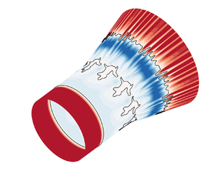
The hollow-cylinder/flare geometry is shown in figure 1. The length of the cylinder is set to L = 0.1 m. The cylinder radius R is varied to investigate the axisymmetric effects, while the flare deflection angle α is adjusted to generate different stages of flow separation. Three typical cylinder radii are considered here: R/L = 0.2, 0.5 and 1.0. Numerical simulations and stability analysis are also performed for the two-dimensional counterpart of the hollow-cylinder/flare model, namely, a compression corner, which represents a limiting case where R/L = ∞. The coordinate system is established with the origin at the centre of the cylinder on the leading-edge plane, the x direction along the cylinder axis, the r direction perpendicular to the axis and the ϕ direction satisfying the right-hand rule.

Figure 1. Schematic view of the hollow-cylinder/flare configuration.
The free-stream flow conditions are taken from the experiment of Leblanc & Ginoux (Reference Leblanc and Ginoux1970): the free-stream streamwise velocity u∞ = 539.5 m s−1, the free-stream temperature T∞ = 143.1 K, the free-stream density ρ∞ = 2.246 × 10⁻² kg m−3, the free-stream Mach number M∞ = 2.25 and the free-stream unit Reynolds number Re∞ = 1.2 × 10⁶ m−1. The wall temperature is set to Tw = 293 K. The air is assumed to be calorically perfect. The specific heat ratio γ is set to 1.4. The dynamic viscosity is calculated from Sutherland's law. The flow-field variables are non-dimensionalized using free-stream quantities.
3. Numerical methods
3.1. Governing equations and base-flow solver
The governing equations are the compressible Navier‒Stokes equations for a calorically perfect gas
 \begin{equation}\frac{{\partial \boldsymbol{U}}}{{\partial t}} + \frac{{\partial \boldsymbol{F}}}{{\partial x}} + \frac{1}{r}\frac{{\partial (r\boldsymbol{G})}}{{\partial r}} + \frac{1}{r}\frac{{\partial \boldsymbol{H}}}{{\partial \phi }} = \frac{1}{r}\boldsymbol{Q},\end{equation}
where U is the vector of conserved variables, F, G and H are the vectors of fluxes and Q is the vector of source terms. See Hao et al. (Reference Hao, Fan, Cao and Wen2022) for detailed expressions of the vectors.
The base-flow solutions are obtained using an in-house multiblock parallel finite-volume solver called PHAROS (Hao, Wang & Lee Reference Hao, Wang and Lee2016; Hao & Wen Reference Hao and Wen2020). The inviscid fluxes are calculated by the modified Steger–Warming scheme (MacCormack Reference MacCormack2014). The scheme is extended to second order by the monotone upstream-centred schemes for conservation law reconstruction (van Leer Reference Van Leer1979). The viscous fluxes are computed using the second-order central difference. An implicit line relaxation method (Wright, Candler & Bose Reference Wright, Candler and Bose1998) is used for pseudo-time stepping.
The free-stream conditions are implemented at the upper and left boundaries, while zero-order extrapolations of flow variables are used for the outlet boundary. The wall is set as no slip and isothermal. The Courant–Friedrichs–Lewy number is set to 103 for pseudo-time stepping. The numerical convergence is determined for a steady state when the density residual decays by more than nine orders of magnitude and the size of the separation region remains constant in successive iterations.
3.2. Global stability analysis
The onset of three-dimensionality is investigated by evaluating the stability of the axisymmetric base flow to azimuthally periodic perturbations; U is divided into an axisymmetric steady solution and a three-dimensional small-amplitude disturbance as
 \begin{equation}\boldsymbol{U}(x,r,\phi ,t) = \bar{\boldsymbol{U}}(x,r) + \boldsymbol{U^{\prime}}(x,r,\phi ,t),\end{equation}
where the overbar and prime represent the base-flow and perturbation variables, respectively. Substituting (3.2) into (3.1) gives the linearized Navier–Stokes (LNS) equations. The parameter U′ is expressed in the following modal form:
 \begin{equation}\boldsymbol{U^{\prime}}(x,r,\phi ,t) = \hat{\boldsymbol{U}}(x,r)\ \textrm{exp}[ - \textrm{i}\omega t + \textrm{i}m\phi ],\end{equation}
where  $\hat{\boldsymbol{U}}$, ω and m denote the axisymmetric eigenfunction, eigenvalue and azimuthal wavenumber, respectively. Here, $m=2{\rm \pi}{/}\lambda$, where λ is the azimuthal wavelength. Note that m must be an integer with m = 0 representing an axisymmetric mode. Substituting (3.3) into the LNS equations and discretizing the result with a second-order finite-volume scheme (Hao et al. Reference Hao, Fan, Cao and Wen2022) yields an eigenvalue problem
 \begin{equation}{\boldsymbol{\mathsf{A}}}\hat{\boldsymbol{U}} = \omega \hat{\boldsymbol{U}},\end{equation}
where  $\boldsymbol{\mathsf{A}} $ is the global matrix composed of Jacobians of the inviscid and viscous fluxes and source terms. In the discretization, the modified Steger–Warming scheme is applied to obtain the inviscid fluxes near discontinuities detected by a shock sensor (Hendrickson, Kartha & Candler Reference Hendrickson, Kartha and Candler2018), while a central scheme is implemented in smooth regions to suppress numerical dissipation (Hao et al. Reference Hao, Cao, Wen and Olivier2021). The second-order central difference is employed for the viscous fluxes. The boundary conditions are consistent with those in the base-flow simulation. The implicitly restarted Arnoldi method implemented in ARPACK (Sorensen et al. Reference Sorensen, Lehoucq, Yang and Maschhoff1996) is employed to solve the eigenvalue problem for a given m. Sponge layers are set near the inflow and outflow boundaries to avoid the reflection of perturbations (Mani Reference Mani2012). The real and imaginary parts of the eigenvalues, ωr and ωi, represent the angular frequency and growth rate of the perturbation, respectively. An unstable mode is indicated by a positive ωi. Note that the spanwise wavenumber β is used in the planar regime.
3.3. Triple-deck theory
To theoretically describe the behaviours of flow separation, Neiland (Reference Neiland1969) and Stewartson & Williams (Reference Stewartson and Williams1969) proposed the supersonic triple-deck theory using asymptotic analysis. The interaction region is divided into three parts (a lower deck, a middle deck and an upper deck) dominated by varying governing equations. The upper deck with a vertical length scale of O(Re −3/8) governed by the Prandtl–Glauert equations is inviscid and irrotational, whereas the middle deck with a vertical length scale of O(Re −1/2) is inviscid and rotational. In the upper and middle decks, simple analytical solutions are obtained (Rizzetta, Burggraf & Jenson Reference Rizzetta, Burggraf and Jenson1978). In the lower deck with a vertical length scale of O(Re −5/8), where the flow is viscous and incompressible, the governing equations are reduced to the incompressible boundary-layer equations by introducing the following scaled variables (Rizzetta et al. Reference Rizzetta, Burggraf and Jenson1978; Ruban Reference Ruban1978; Gittler & Kluwick Reference Gittler and Kluwick1987):
 \begin{gather}\left.
{\begin{array}{*{20}{c@{}}} {{x^\ast } = R{e^{3/8}}{C^{ -
3/8}}{\lambda^{5/4}}{{(M_\infty^2 - 1)}^{3/8}}{{\left(
{\dfrac{{{T_w}}}{{{T_\infty }}}} \right)}^{ -
3/2}}\dfrac{{x - L}}{L},}\\ {{y^\ast } = R{e^{5/8}}{C^{ -
5/8}}{\lambda^{3/4}}{{(M_\infty^2 - 1)}^{1/8}}{{\left(
{\dfrac{{{T_w}}}{{{T_\infty }}}} \right)}^{ -
3/2}}\dfrac{{y - R}}{L},}\\ {{p^\ast } = R{e^{1/4}}{C^{ -
1/4}}{\lambda^{ - 1/2}}{{(M_\infty^2 - 1)}^{1/4}}\dfrac{{p
- {p_\infty }}}{{{\rho_\infty }u_\infty^2}},}\\
{{\alpha^\ast } = R{e^{1/4}}{C^{ - 1/4}}{\lambda^{ -
1/2}}{{(M_\infty^2 - 1)}^{ - 1/4}}\alpha ,}\\ {{R^\ast } =
R{e^{3/8}}{C^{ - 3/8}}{\lambda^{5/4}}{{(M_\infty^2 -
1)}^{7/8}}{{\left( {\dfrac{{{T_w}}}{{{T_\infty }}}}
\right)}^{ - 3/2}}\dfrac{R}{L},}\\ {{u^\ast } =
R{e^{1/8}}{C^{ - 1/8}}{\lambda^{ - 1/4}}{{(M_\infty^2 -
1)}^{1/8}}{{\left( {\dfrac{{{T_w}}}{{{T_\infty }}}}
\right)}^{ - 1/2}}\dfrac{u}{{{u_\infty }}},}\\ {{v^\ast } =
R{e^{3/8}}{C^{ - 3/8}}{\lambda^{ - 3/4}}{{(M_\infty^2 -
1)}^{ - 1/8}}{{\left( {\dfrac{{{T_w}}}{{{T_\infty }}}}
\right)}^{ - 1/2}}\dfrac{v}{{{u_\infty }}},}\\ {{A^\ast } =
R{e^{5/8}}{C^{ - 5/8}}{\lambda^{3/4}}{{(M_\infty^2 -
1)}^{1/8}}{{\left( {\dfrac{{{T_w}}}{{{T_\infty }}}}
\right)}^{ - 3/2}}\dfrac{A}{L},} \end{array}}
\right\}\end{gather}
\begin{gather}\left.
{\begin{array}{*{20}{c@{}}} {{x^\ast } = R{e^{3/8}}{C^{ -
3/8}}{\lambda^{5/4}}{{(M_\infty^2 - 1)}^{3/8}}{{\left(
{\dfrac{{{T_w}}}{{{T_\infty }}}} \right)}^{ -
3/2}}\dfrac{{x - L}}{L},}\\ {{y^\ast } = R{e^{5/8}}{C^{ -
5/8}}{\lambda^{3/4}}{{(M_\infty^2 - 1)}^{1/8}}{{\left(
{\dfrac{{{T_w}}}{{{T_\infty }}}} \right)}^{ -
3/2}}\dfrac{{y - R}}{L},}\\ {{p^\ast } = R{e^{1/4}}{C^{ -
1/4}}{\lambda^{ - 1/2}}{{(M_\infty^2 - 1)}^{1/4}}\dfrac{{p
- {p_\infty }}}{{{\rho_\infty }u_\infty^2}},}\\
{{\alpha^\ast } = R{e^{1/4}}{C^{ - 1/4}}{\lambda^{ -
1/2}}{{(M_\infty^2 - 1)}^{ - 1/4}}\alpha ,}\\ {{R^\ast } =
R{e^{3/8}}{C^{ - 3/8}}{\lambda^{5/4}}{{(M_\infty^2 -
1)}^{7/8}}{{\left( {\dfrac{{{T_w}}}{{{T_\infty }}}}
\right)}^{ - 3/2}}\dfrac{R}{L},}\\ {{u^\ast } =
R{e^{1/8}}{C^{ - 1/8}}{\lambda^{ - 1/4}}{{(M_\infty^2 -
1)}^{1/8}}{{\left( {\dfrac{{{T_w}}}{{{T_\infty }}}}
\right)}^{ - 1/2}}\dfrac{u}{{{u_\infty }}},}\\ {{v^\ast } =
R{e^{3/8}}{C^{ - 3/8}}{\lambda^{ - 3/4}}{{(M_\infty^2 -
1)}^{ - 1/8}}{{\left( {\dfrac{{{T_w}}}{{{T_\infty }}}}
\right)}^{ - 1/2}}\dfrac{v}{{{u_\infty }}},}\\ {{A^\ast } =
R{e^{5/8}}{C^{ - 5/8}}{\lambda^{3/4}}{{(M_\infty^2 -
1)}^{1/8}}{{\left( {\dfrac{{{T_w}}}{{{T_\infty }}}}
\right)}^{ - 3/2}}\dfrac{A}{L},} \end{array}}
\right\}\end{gather} \begin{gather}Re = \frac{{{\rho _\infty }{u_\infty }L}}{{{\mu _\infty }}},\quad C = \frac{{{\mu _w}{T_\infty }}}{{{\mu _\infty }{T_w}}}.\end{gather}
Here, x* and y* are the scaled streamwise and radial coordinates, respectively; p* is the scaled pressure; α* is the scaled deflection angle; R* is the scaled cylinder radius; u* and v* are the scaled axial and radial velocities, respectively; A* is the scaled displacement thickness; Re is the Reynolds number; C is the Chapman–Rubesin parameter; λ is a value determined by the slope of the velocity profile at the wall in the coming boundary layer. For a Blasius boundary layer, λ equals 0.33206. For R/L = 0.2, 0.5 and 1.0, R* = 4.948, 12.37 and 24.74, respectively.
According to Gittler & Kluwick (Reference Gittler and Kluwick1987), the governing equations for hollow-cylinder/flare flows in the lower deck are
 \begin{equation}\left. {\begin{array}{*{20}{c@{}}} {\dfrac{{\partial {u^\ast }}}{{\partial {t^\ast }}} + {u^\ast }\dfrac{{\partial {u^\ast }}}{{\partial {x^\ast }}} + {v^\ast }\dfrac{{\partial {u^\ast }}}{{\partial {y^\ast }}} =- \dfrac{{\textrm{d}{p^\ast }}}{{\textrm{d}\kern0.7pt {x^\ast }}} + \dfrac{{{\partial^2}{u^\ast }}}{{\partial {y^\ast }^2}},}\\ {\dfrac{{\partial {u^\ast }}}{{\partial {x^\ast }}} + \dfrac{{\partial {v^\ast }}}{{\partial {y^\ast }}} = 0,} \end{array}} \right\}\end{equation}
with the following boundary conditions: u* = v* = 0 for y* = F*(x*); u* = y* + A*(x*) as y* → ∞; u* = y* as x* → −∞. The shape function F* is defined as
 \begin{equation}{F^\ast
}({x^\ast }) = \left\{ {\begin{array}{@{}l@{\quad}l@{}}
0&{{x^\ast } < - \varepsilon, }\\
{\dfrac{{{\alpha^\ast }}}{{4\varepsilon }}({x^\ast }^2 +
2\varepsilon {x^\ast } + {\varepsilon^2})}&{ - \varepsilon
\le {x^\ast } \le \varepsilon }\\
{{\alpha^\ast }{x^\ast }}&{{x^\ast } > \varepsilon, }
\end{array}}
\right.,\end{equation}
\begin{equation}{F^\ast
}({x^\ast }) = \left\{ {\begin{array}{@{}l@{\quad}l@{}}
0&{{x^\ast } < - \varepsilon, }\\
{\dfrac{{{\alpha^\ast }}}{{4\varepsilon }}({x^\ast }^2 +
2\varepsilon {x^\ast } + {\varepsilon^2})}&{ - \varepsilon
\le {x^\ast } \le \varepsilon }\\
{{\alpha^\ast }{x^\ast }}&{{x^\ast } > \varepsilon, }
\end{array}}
\right.,\end{equation}where ε is the rounding parameter with ε = 0 representing a sharp corner. All subsequent triple-deck calculations are performed with ε = 1. With Prandtl's transposition theorem
 \begin{equation}\left. {\begin{array}{*{20}{c@{}}} {{z^\ast } = {y^\ast } - {F^\ast }({x^\ast }),}\\ {{w^\ast } = {v^\mathrm{\ast }} - {u^\mathrm{\ast }}{F^\ast }^\prime ({x^\mathrm{\ast }}),} \end{array}} \right\}\end{equation}
the above governing equations are written as
 \begin{equation}\left. {\begin{array}{*{20}{c@{}}} {{u^\mathrm{\ast }}\dfrac{{\partial {u^\mathrm{\ast }}}}{{\partial {x^\mathrm{\ast }}}} + {w^\ast }\dfrac{{\partial {u^\ast }}}{{\partial {z^\ast }}} =- \dfrac{{\textrm{d}{p^\ast }}}{{\textrm{d}\kern0.7pt {x^\ast }}} + \dfrac{{{\partial^2}{u^\ast }}}{{\partial {z^\ast }^2}},}\\ {\dfrac{{\partial {u^\ast }}}{{\partial {x^\ast }}} + \dfrac{{\partial {w^\ast }}}{{\partial {z^\ast }}} = 0,} \end{array}} \right\}\end{equation}
with the boundary conditions: u* = w* = 0 at z* = 0; u* → z* + A*(x*) + F*(x*) for z* → ∞; u* → z* for x* → −∞. The interaction law describing the correlation between the induced pressure and displacement thickness is given by
 \begin{equation}{p^\ast }({x^\ast }) =- \frac{{\partial {A^\ast }}}{{\partial {x^\ast }}} + \frac{1}{{{R^\ast }}}\int_{ - \infty }^x {W\Big( {\frac{{x - \xi }}{{{R^\ast }}}} \Big){A^\ast }^\prime (\xi )\,\textrm{d}\xi } .\end{equation}
Here,
 \begin{equation}W(z) = \int_0^\infty {\frac{{{\textrm{e}^{ - \lambda z}}}}{{K_1^2(\lambda ) + {{\rm \pi} ^2}I_1^2(\lambda )}}\frac{{\textrm{d}\lambda }}{\lambda }} \end{equation}
is the function introduced by Ward (Reference Ward1948), where I 1 and K 1 are the modified Bessel functions of the first kind and the second kind, respectively.
The steady solutions of (3.10) are obtained by an explicit finite difference method that is first order in time integration and second order in spatial discretization. Specifically, a second-order backward or forward difference scheme is applied to approximate the streamwise convection term depending on whether u* is positive or negative. The scaled wall shear stress is obtained by τ* = ∂u*/∂y*.
4. Results
4.1. General flow features
Base flows are obtained for a hollow cylinder/flare with a series of cylinder radii and flare deflection angles and its two-dimensional counterpart with different ramp angles. For convenience, the critical deflection angles for incipient and secondary separation are denoted by α 1 and α 2, respectively.
The skin friction coefficient Cf and surface pressure coefficient Cp are defined as
 \begin{equation}{C_f} = \frac{{{\tau _w}}}{{0.5{\rho _\infty }u_\infty ^2}},\quad {C_p} = \frac{{{p_w}}}{{0.5{\rho _\infty }u_\infty ^2}},\end{equation}
where τw and pw are the skin shear stress and surface pressure, respectively. The locations of the separation and reattachment points are identified when Cf crosses zero upstream and downstream, respectively. The size of the separation region Lsep is measured from the separation point to the reattachment point along the x-axis. A grid independence study (see Appendix A) shows that 600 × 350 grid points are sufficient for both CFD simulations and GSA. The triple-deck calculations are performed for the axisymmetric and planar flows with 1000 × 200 and 800 × 200 grid points, respectively. A good agreement is observed between the obtained triple-deck solutions and data in the literature (see Appendix B).
Figure 2 presents the skin friction curves at various deflection angles for different cylinder radii R/L = 0.2, 0.5, 1.0 and ∞. The open symbols represent the separation and reattachment points. The enlarged views near the juncture are also displayed. Following an initial decrease upstream of separation due to the development of the laminar boundary layer, Cf experiences a rapid decay near the separation point to the first local minimum and then a gradual growth along the cylinder. Downstream of the juncture, a downward trend of Cf to the second local minimum is observed in the separation region. After the noticeable second local minimum, the skin friction progressively increases around the reattachment point. The existence of two local minima in Cf inside the separation zone indicates a fully separated flow. As α is increased, the extent of the separation zone accordingly grows. The magnitudes of both the second minimum and the local peak near the juncture also increase with increasing α. These features are similar to the findings in compression corner flows (Smith & Khorrami Reference Smith and Khorrami1991; Korolev, Gajjar & Ruban Reference Korolev, Gajjar and Ruban2002; Shvedchenko Reference Shvedchenko2009; Gai & Khraibut Reference Gai and Khraibut2019). Beyond a threshold deflection angle α 2, secondary separation occurs, which is characterized by a positive local peak near the juncture. The secondary bubble emerges at 15° ≤ α 2 ≤ 16° for R/L = 0.2. When the cylinder radius is increased to R/L = 0.5 and 1.0, α 2 decreases to 14°–15° and 13°–14°, respectively. It is observed that the emergence of secondary separation is delayed to a higher deflection angle when the cylinder radius is decreased. With respect to the compression corner flow (R/L = ∞), the critical ramp angle for secondary separation is 11°–12°, which is lower than those for the axisymmetric flows. The above results can be interpreted by the triple-deck theory through the scaled deflection angle α* to determine the critical angles for incipient separation and secondary separation. For R/L = ∞ (R* = ∞), secondary separation occurs at α* = 4.51–4.92. As the cylinder radius is decreased to R/L = 1.0, 0.5 and 0.2 (R* = 24.74, 12.37 and 4.948), the occurrence of secondary separation is delayed to α* = 5.33–5.74, 5.74–6.15 and 6.15–6.57, respectively. Additional CFD simulations show that the critical angles for incipient separation are α* = 1.64–2.05 for R* = 4.948 and 12.37 and α* = 1.23–1.64 for R* = 24.74 and ∞.

Figure 2. The skin friction coefficient distributions for (a) R/L = 0.2, (b) R/L = 0.5, (c) R/L = 1.0 and(d) R/L = ∞ at different deflection angles with enlarged views near the juncture (PHAROS). Open symbols: separation and reattachment points. Horizontal dashed line: zero skin friction. Vertical dashed line: juncture.
As seen in figure 2, the length of the separation region and the magnitude of the second minimum in Cf depend on the deflection angle α for a given cylinder radius. Burggraf (Reference Burggraf1975) and Korolev et al. (Reference Korolev, Gajjar and Ruban2002) showed a linear dependence between  $L_{sep}^\ast $ and α *3/2 for a compression corner based on the triple-deck theory. Here, $L_{sep}^\ast $ is plotted versus α *3/2 for varying scaled cylinder radii R* in figure 3(a). The linear dependence still holds for hollow-cylinder/flare flows with the slope decreasing as the cylinder radius is decreased. Korolev et al. (Reference Korolev, Gajjar and Ruban2002) also noted that the magnitude of the wall shear stress minimum ahead of reattachment |τw ,min| is proportional to α* for a compression corner flow. Figure 3(b) presents the variations in |Cf ,min| against α* for the considered cases. It is confirmed that a linear relationship between |Cf ,min| and α* is satisfied for both the compression corner and hollow-cylinder/flare flows.

Figure 3. The (a) scaled length of the separation region as a function of α *3/2 and (b) magnitude of the second minimum in Cf as a function of α* for axisymmetric and planar configurations (PHAROS).
In figure 4, the scaled length of the separation region and the magnitude of the second skin friction minimum are plotted against the scaled cylinder radius for varying deflection angles. In figure 4(a), as the cylinder radius is increased, the size of the separation bubble experiences an increase and eventually converges to the planar results denoted by the dashed lines. Similarly, the magnitude of the friction minimum grows with increasing R* and approaches the planar data in figure 4(b).

Figure 4. The (a) scaled length of the separation region and (b) magnitude of the second minimum in Cf as a function of R* for varying deflection angles (PHAROS). Horizontal dashed line: the limiting planar results.
The surface pressure coefficients for various cylinder radii and deflection angles are shown in figure 5. The initial rise in surface pressure upstream of the separation point is governed by the free-interaction process (Chapman, Kuehn & Larson Reference Chapman, Kuehn and Larson1958). Downstream of separation, a pressure plateau forms, and both its size and magnitude increase with increasing α. A small ‘dip’ can be observed near the juncture at the end of the pressure plateau for large α, which becomes progressively noticeable as α is increased. This local drop indicates a local low-pressure region near the juncture, which is consistent with the observations in compression corner and double-cone flows (Smith & Khorrami Reference Smith and Khorrami1991; Korolev et al. Reference Korolev, Gajjar and Ruban2002; Gai & Khraibut Reference Gai and Khraibut2019; Hao et al. Reference Hao, Fan, Cao and Wen2022). Near the reattachment point, Cp experiences a drastic rise, which becomes steeper with increasing α. This pressure climb continues until Cp reaches the peak value, which grows with α.

Figure 5. The distributions of the surface pressure coefficient for (a) R/L = 0.2, (b) R/L = 0.5, (c) R/L = 1.0 and (d) R/L = ∞ with different deflection angles (PHAROS). Open symbols: separation and reattachment points. Vertical dashed line: juncture.
For R/L = 0.5, figure 6 presents the density gradients in the separation region and the non-dimensional pressure scaled by  ${\rho _\infty }u_\infty ^2$ in the juncture region at α = 14° and 15°. At α = 14°, the primary vortex core is located over the flare surface downstream of the juncture, and the secondary separation bubble is not seen. At α = 15°, a secondary vortex emerges beneath the primary bubble close to the juncture, while the primary bubble fragments into two vortices. A smaller secondary bubble also appears on the flare. At α = 14°, there is a low-pressure zone near the vortex core, which may balance the centrifugal force of a fluid element rotating about the core (Jeong & Hussain, Reference Jeong and Hussain1995). The ‘dip’ in Cp is assumed to reflect this low-pressure zone on the flare. As α grows, the low pressure near the primary vortex core remains almost unchanged, while the pressure in the upstream part of the separation zone increases in accordance with the change in the plateau pressure (see figure 5).

Figure 6. Contours of (a) density gradient magnitude and (b) non-dimensional pressure scaled by  ${\rho _\infty }u_\infty ^2$ with streamlines superimposed for R/L = 0.5 at α = 14° (left column) and 15° (right column) (PHAROS).
The axisymmetric effects are then studied by comparing the solutions with different cylinder radii. Figure 7 presents the distributions of Cf and Cp at two deflection angles, α = 5° and 13°. The open symbols represent the separation and reattachment points. A detailed view of the skin friction distributions near the juncture at α = 13° is also shown here. As α = 5° is slightly higher than the incipient separation angle, only a marginal separation region is observed, and a pressure plateau has not yet formed. At α = 13°, the emergence of two local minima in Cf and a constant plateau in Cp suggests a large separation region. As R is decreased, the surface pressure upstream of separation gradually decreases (Kluwick et al. Reference Kluwick, Gittler and Bodonyi1984; Kluwick, Gittler & Bodonyi Reference Kluwick, Gittler and Bodonyi1985), whereas the skin friction shows an opposite trend (White & Majdalani Reference White and Majdalani2006). The length of the separation region and the magnitude of the local minima of Cf both increase with R for a fixed α, which corresponds to figure 4. Furthermore, the plateau and peak pressures both grow with increasing R. The pressure overshoot on the flare surface is due to the strong compression waves induced by flow reattachment. In fact, if the flow is inviscid, the pressure immediately downstream of the juncture obeys the oblique shock relations. Due to the axisymmetric effects on the viscous–inviscid interaction, the oblique shock solution can never be achieved. When R is progressively increased to recover the two-dimensional case, the surface pressure far downstream of reattachment increasingly approaches the value predicted by the oblique shock relations. Conversely, as the cylinder body becomes slenderer, the decay of Cp to a lower limit value determined by the conical shock relations becomes more rapid. Such trends in Cp on the flare are indicative of the axisymmetric effects.

Figure 7. The distributions of the skin friction coefficient (left column) and surface pressure coefficient (right column) for varying cylinder radii at (a) α = 5° and (b) α = 13° (PHAROS). Horizontal dashed line: zero skin friction for Cf, pressure predicted by the oblique shock relations (upper) and conical shock relations (lower) for Cp. Vertical dashed line: juncture.
Figure 7 demonstrates that for a given α, the axisymmetric effects decay with increasing R, and the separation and reattachment processes are milder in an axisymmetric flow than in its two-dimensional counterpart. The length of the separation region, the peak and plateau pressures and the skin friction minima increase with increasing R and eventually recover to the two-dimensional solutions. Furthermore, the occurrence of both incipient and secondary separation is postponed with decreasing R, which is indicative of more pronounced transverse curvature effects. As R is decreased, the axisymmetric effects lead to a slightly higher Cf upstream of separation and a decreasing pressure overshoot downstream of reattachment, thus reducing the size of the separation bubble and delaying the occurrence of separation.
Despite a general overestimation of the size of the separation region (Katzer Reference Katzer1989), the triple-deck theory is accurate in anticipating the occurrence of flow separation. Figure 8 presents the distributions of scaled wall shear stress for hollow-cylinder/flare flows and compression corner flows by solving the triple-deck equations at varying α*. Note that, due to the rounded juncture, the minimum shear stress emerges upstream of the juncture when α* is small (Kluwick et al. Reference Kluwick, Gittler and Bodonyi1984). The distributions of wall shear stress for axisymmetric flows are generally consistent with those for two-dimensional flows. The incipient separation emerges at  $\alpha _1^\ast= 2.05\unicode{x2013} 2.46$ for R* = 4.948 and 12.37, and 1.64–2.05 for R* = 24.74. For compression corner flows, the critical angle for incipient separation is $1.64 \le \alpha _1^\ast \le 2.05$. The exact calculations give $\alpha _1^\ast \approx 1.85$, which is in reasonable agreement with the values obtained by Cassel, Ruban & Walker (Reference Cassel, Ruban and Walker1995), Grisham, Dennis & Lu (Reference Grisham, Dennis and Lu2018) and Exposito, Gai & Neely (Reference Exposito, Gai and Neely2021). This value is higher than the typical value of 1.57 (Rizzetta et al. Reference Rizzetta, Burggraf and Jenson1978; Ruban Reference Ruban1978) due to a rounded corner. The critical incipient separation angle for an axisymmetric flow is much higher than that for the corresponding planar problem and increases with decreasing cylinder radius, which corresponds well with the findings of Huang & Inger (Reference Huang and Inger1983) and Kluwick et al. (Reference Kluwick, Gittler and Bodonyi1984). Similar trends are observed for the occurrence of secondary separation. For the planar case, secondary separation is observed at $4.10 \le \alpha _2^\ast \le 4.51$, which agrees well with the results of Smith & Khorrami (Reference Smith and Khorrami1991), Korolev et al. (Reference Korolev, Gajjar and Ruban2002), Shvedchenko (Reference Shvedchenko2009) and Gai & Khraibut (Reference Gai and Khraibut2019). For the axisymmetric flow, the critical angle of secondary separation decreases from 6.15–6.57 for R* = 4.948 to 5.33–5.74 for R* = 12.37 and 4.92–5.33 for R* = 24.74. In effect, the triple-deck solutions show that the critical deflection angles of both incipient and secondary separation decrease with increasing cylinder radius and eventually approach the values for the compression corner case. Although triple-deck theory generally provides a slight overprediction of the incipient separation angles and a marginal underprediction of the secondary separation angles, the triple-deck solutions exhibit the same overall trends as the CFD solutions in terms of the axisymmetric effects.

Figure 8. The scaled wall shear stress distributions obtained by the triple-deck theory for different cylinder radii (a) R* = 4.948, (b) R* = 12.37, (c) R* = 24.74 and (d) R* = ∞ at various deflection angles (triple-deck solutions). Vertical dashed line: juncture. Horizontal dashed line: scaled wall shear stress of zero and one.
It is significant to quantitatively assess the accuracy of the triple-deck theory in terms of estimating the length of the separation region. Despite satisfactory qualitative results, Burggraf et al. (Reference Burggraf, Rizzetta, Werle and Vatsa1979) found that the quantitative accuracy was only obtained at very high Reynolds numbers. Katzer (Reference Katzer1989) indicated an overprediction of the separation region for finite Reynolds numbers. The discrepancy was found to increase with increasing Mach number and decreasing Reynolds number. With respect to the influence of wall temperature, Exposito et al. (Reference Exposito, Gai and Neely2021) revealed an overestimation of the triple-deck theory for Tw/T 0 ≥ 0.15 and an underestimation for Tw/T 0 ≤ 0.15. Figure 9 compares the scaled length of the separation region obtained by both triple-deck and CFD solutions. Similar to figure 3, the triple-deck results exhibit a linear trend with α *3/2 for both planar and axisymmetric cases in figure 9(a). However, the noticeable discrepancy of the triple-deck and base-flow results in their slopes indicates a general overprediction of the triple-deck theory. The overestimation substantially grows with α because the linearized theory assumed in triple-deck theory no longer holds for higher α. The influence of cylinder radius is taken into consideration in figure 9(b). The discrepancy between the base-flow results and the triple-deck data increases as the cylinder radius is increased. The triple-deck theory in the axisymmetric regime assumes that the scaled body radius satisfies R* ∼ O(1) (Huang & Inger Reference Huang and Inger1983; Kluwick et al. Reference Kluwick, Gittler and Bodonyi1984). Therefore, a better estimation is obtained for a slightly smaller body radius (Kluwick et al. Reference Kluwick, Gittler and Bodonyi1985). As the cylinder radius is increased, the interaction law which relates the pressure and displacement thickness is not appropriate for consideration, thus leading to the overestimation of the length of the separation region. The hot wall (Tw/T 0 = 1.02) in the present instance also contributes to the overestimation in figure 9 (Exposito et al. Reference Exposito, Gai and Neely2021).

Figure 9. The scaled length of the separation region as a function of (a) α *3/2 for R* = 12.37 and ∞ and (b) R* for a constant deflection angle α* = 3.69 (PHAROS and triple-deck solutions). Open symbols: base-flow data. Solid symbols: triple-deck data. Horizontal dashed line in (b): limiting planar results.
The above discussion reveals that the triple-deck theory provides a satisfactory prediction for the occurrence of incipient and secondary separation. However, this asymptotic theory exhibits limitations in quantitatively estimating the length of the separation region.
4.2. Occurrence of global instability
To identify the global stability of azimuthally periodic perturbations imposed on the base flows, GSA is performed over a wide range of azimuthal wavenumbers with a series of cylinder radii and flare deflection angles.
The global instability of the appropriate compression corner flow is considered first. Figure 10 shows the growth rates of the most unstable modes as a function of the spanwise wavenumber for various deflection angles. At the lowest deflection angle α = 9°, only stable modes are observed. At α = 10°, the compression corner flow becomes globally unstable with the presence of a stationary unstable mode whose largest growth rate occurs at βL = 16.9 (λ/L = 0.37). When α is increased to 11°, the unstable mode is shifted to a smaller wavenumber of βL = 14.1 (λ/L = 0.45). As α is further increased, more unstable modes gradually emerge. At α = 12°, three unstable modes including two stationary unstable modes (modes 1 and 3) and an oscillatory unstable mode (mode 2) are captured by the GSA. The mode shown in figure 10 corresponds to mode 1, which has the largest growth rate among the three modes. At α = 13°, four unstable modes exist, including two stationary modes and two oscillatory modes. The strongest mode reaches its maximum growth rate at βL = 67.9 (λ/L = 0.093).

Figure 10. Variations in the growth rates of the most unstable modes as a function of spanwise wavenumber at different flare deflection angles for R/L = ∞ (GSA). Vertical dashed line: the most unstable wavenumber. Horizontal dashed line: zero growth rate.
The growth rates and angular frequencies of the three unstable modes captured at α = 12° are plotted as a function of the spanwise wavenumber in figure 11.Modes 1 and 2 reach their maximum growth rates at βL = 60.5 (λ/L = 0.104) and βL = 66.7 (λ/L = 0.094), respectively. The weaker stationary mode (mode 3) with the growth rates peaking at approximately βL = 11.2 (λ/L = 0.56) corresponds to the stationary modes observed at α = 10° and 11°. Figure 12 presents the contours of the real part of the pressure perturbation p′ and spanwise velocity perturbation w′ for modes 1 and 2 at their respective most unstable spanwise wavenumbers. The features of the pressure and spanwise velocity perturbations are consistent with previous findings in compression corner flows (Cao et al. Reference Cao, Hao, Klioutchnikov, Olivier and Wen2021; Hao et al. Reference Hao, Cao, Wen and Olivier2021). The pressure perturbations mainly exist in the downstream half of the separation zone, with the positive and negative parts periodically coupled to each other. The wave-like structures further stretch downstream of the reattachment.

Figure 11. Variations in (a) growth rates and (b) frequencies of the unstable modes as a function of spanwise wavenumber for R/L = ∞ at α = 12° (GSA). Vertical dashed line: the most unstable wavenumber. Horizontal dashed line: zero growth rate and angular frequency.

Figure 12. Real parts of (a) the spanwise velocity perturbation and (b) pressure perturbation for mode 1 (left column) with βL = 60.5 and mode 2 (right column) with βL = 66.7 at α = 12° for the two-dimensional problem (GSA). The contour levels are uniformly distributed between ±0.1 of the maximum |w′| and |p′|, respectively.
For an intermediate radius R/L = 0.5, figure 13 presents the growth rates of the captured dominant unstable modes as a function of azimuthal wavenumber at various deflection angles. Note that these dominant unstable modes shown in figure 13 are all stationary. At α = 11°, the flow is globally stable. A globally unstable mode appears at α = 12°. At α = 13°, the peak growth rate further increases and shifts to a slightly smaller wavenumber, which corresponds to the trend shown in figure 10. Two stationary unstable modes are observed at α = 14°. One belongs to the same family as those at lower angles (not shown), while the other becomes dominant with the most unstable azimuthal wavenumber of m = 36. A further slight increase in the flare angle has profound consequences on the global instability. At α = 15°, four unstable modes are captured. The maximum growth rate of the most unstable mode occurs at m = 40. Recall that the secondary separation angle is 14°–15° for R/L = 0.5. The growth rate of the most unstable mode increases with α. At α = 12° and 13°, there is only one unstable stationary mode with a relatively small wavenumber. As α approaches and surpasses α 2, the flow is strongly destabilized and dominated by a new stationary mode with a much larger wavenumber, which is consistent with the compression corner flow.

Figure 13. Variations in the growth rates of the most unstable modes as a function of azimuthal wavenumber at different flare deflection angles for R/L = 0.5 (GSA). Vertical dashed line: the most unstable wavenumber. Horizontal dashed line: zero growth rate.
For R/L = 0.5, the flow is strongly destabilized at α = 15°. The growth rates and angular frequencies of the four unstable modes against the azimuthal wavenumber are plotted in figure 14. Note that mode 1 is the mode shown in figure 13 at α = 15°. The distributions of angular frequencies suggest that modes 1 and 3 are stationary, whereas modes 2 and 4 are oscillatory. The growth rate of mode 1 peaks at m = 40, whereas mode 2 reaches its maximum growth rate at a slightly larger wavenumber m = 42. The dominant frequency of mode 2 at m = 42 is approximately f = ωr/2 ${\rm \pi}$ = 3.0 kHz ( f L/u∞ = 0.56). Modes 3 and 4 reach their maximum growth rates at considerably lower azimuthal wavenumbers m = 8 and 14, respectively. Note that mode 3 is associated with the stationary unstable modes captured at α = 12°, 13° and 14°, as shown in figure 13.

Figure 14. Variations in (a) growth rates and (b) angular frequencies of the most unstable modes as a function of azimuthal wavenumber at α = 15° for R/L = 0.5 (GSA). Vertical dashed line: the most unstable wavenumber. Horizontal dashed line: zero growth rate and angular frequency.
For R/L = 0.5 and α = 15°, figure 15 presents the contours of the real parts of pressure perturbation p′ and azimuthal velocity perturbation w′ for modes 1 and 2 at m = 40 and 42, respectively. Modes 1 and 2 are structurally similar to the dominant stationary and oscillatory unstable modes shown in figure 12 and the unstable modes observed in supersonic double-wedge flows, compression corner flows, double-cone flows and hollow-cylinder/flare flows (Sidharth et al. Reference Sidharth, Dwivedi, Candler and Nichols2018; Cao et al. Reference Cao, Hao, Klioutchnikov, Olivier and Wen2021; Hao et al. Reference Hao, Cao, Wen and Olivier2021, Reference Hao, Fan, Cao and Wen2022; Lugrin et al. Reference Lugrin, Beneddine, Garnier and Bur2021a). The unstable modes are attributed to the separated flow, and they are identical in nature. Appendix C presents the distributions of streamwise and radial velocity perturbations, density perturbations and temperature perturbations for modes 1 and 2.

Figure 15. Real parts of (a) the pressure perturbations and (b) azimuthal velocity perturbations for mode 1 (left column) at m = 40 and mode 2 at m = 42 (right column) for R/L = 0.5 at α = 15° (GSA). The contour levels are uniformly distributed between ±0.1 of the maximum |w′| and |p′|, respectively.
The growth rates of the most unstable modes as a function of azimuthal wavenumber at different deflection angles are shown in figure 16 for R/L = 0.2 and 1.0. For R/L = 0.2, the separated flow becomes unstable at α = 13°, which is higher than that for R/L = 0.5. As α is increased to 14° and 15°, the stationary unstable mode is observed at m = 5. When α is further increased to 16°, the maximum growth rate of the least stable mode occurs at m = 19. For R/L = 1.0, global instability occurs at α = 11°, which is lower than that for R/L = 0.5. As α is increased to 12°, an unstable mode is observed at m = 18. At α = 13° and 14°, the most unstable modes are shifted to considerably higher wavenumbers m = 66 and 72, respectively. It is observed that the variations of the maximum ωi and corresponding m in different α for R/L = 0.2 and 1.0 are similar to those unveiled for R/L = 0.5. However, the emergence of global instability is suppressed as R is decreased. For R/L = 0.2 and 1.0, a series of stationary and oscillatory unstable modes emerge at higher deflection angles. These obtained modes are similar to the unstable modes presented in figure 15 and thus are not shown here for brevity.

Figure 16. Variations in the growth rates of the most unstable modes as a function of azimuthal wavenumber for (a) R/L = 0.2 and (b) R/L = 1.0 with increasing deflection angles (GSA). Vertical dashed line: the most unstable azimuthal wavenumber. Horizontal dashed line: zero growth rate.
Similarly, the GSA results can be scaled using the triple-deck theory to determine the critical deflection angles where the flow becomes globally unstable. For the planar case R* = ∞, α* = 3.69–4.10, which agrees well with the stability boundary for a compression corner flow by Hao et al. (Reference Hao, Cao, Wen and Olivier2021). For R* = 24.74, 12.37 and 4.948, α* = 4.10–4.51, 4.51–4.92 and 4.92–5.33, respectively. A decrease in cylinder radius postpones the occurrence of global instability. When the deflection angle gradually approaches and exceeds the critical secondary separation angle α 2, the flow is strongly destabilized with the emergence of more unstable modes and a pronounced increase in the growth rate of the most unstable mode.
4.3. Direct numerical simulations
Direct numerical simulations are performed for the canonical case R/L = 0.5 and its planar counterpart R/L = ∞ at α = 15° to verify the foregoing GSA results and illustrate the temporal evolution of three-dimensional structures.
The GSA is similarly performed for the compression corner flow at α = 15°. Since the planar flow is much more unstable than its axisymmetric equivalent, a finer mesh (600 × 450) is used for the base-flow simulations and GSA to ensure grid convergence. The GSA results of the planar case at α = 15° are shown in Appendix D. Note that the three most unstable modes (modes 1, 2 and 3) reach their maximum growth rates at βL = 74, 60 and 72, respectively.
Direct numerical simulations are performed for both axisymmetric and planar flows at α = 15° to verify the GSA results. For the axisymmetric case, the medium mesh (600 × 350) is rotated around the flow axis over an azimuthal angle of 36° with 200 grid cells in the azimuthal (ϕ) direction. This azimuthal angle is chosen because the growth rates of mode 1 and mode 2 peak at m = 40 and 42, respectively. The initial flow field is generated through a duplication of the base flow along the azimuthal direction. Similarly, for the planar case, the mesh with 600 × 450 grid points is extended along the spanwise (z) direction for 42 mm, which corresponds to approximately five wavelengths of mode 1 at R/L = ∞. The 200 grid points are equally spaced in the spanwise direction. The three-dimensional flow field is generated by extending the base-flow solution in the spanwise direction. The inlet and upper boundary conditions are given by the free-stream profiles. Periodic boundary conditions are enforced on the azimuthal/spanwise boundaries. Without introducing any external or internal perturbations, the numerical round-off error is expected to induce global instability. The three-dimensional simulations are conducted using PHAROS with a second-order implicit method (Peterson Reference Peterson2011) for time integration. The physical time step is set to 20 ns for both axisymmetric and planar simulations. To ensure a sufficiently developed flow, the simulated time is set to t = 20 ms (tu∞/L = 108) for R/L = 0.5 and t = 8 ms (tu∞/L = 43) for R/L = ∞.
The evolution of global instability is described by the root mean square of the azimuthal/spanwise velocity (Cao et al. Reference Cao, Hao, Klioutchnikov, Olivier and Wen2021; Hao et al. Reference Hao, Fan, Cao and Wen2022) at a streamwise location, which is defined as
 \begin{equation}{\sigma
_w} = \sqrt{\frac{1}{{{N_r}{N_\phi }}}\sum\limits_{j =
1}^{{N_r}} {\sum\limits_{k = 1}^{{N_\phi }} {{{\left(
{\frac{w}{{{u_\infty }}}} \right)}^2}} } }
\end{equation}
\begin{equation}{\sigma
_w} = \sqrt{\frac{1}{{{N_r}{N_\phi }}}\sum\limits_{j =
1}^{{N_r}} {\sum\limits_{k = 1}^{{N_\phi }} {{{\left(
{\frac{w}{{{u_\infty }}}} \right)}^2}} } }
\end{equation}for the axisymmetric flow and
 \begin{equation}{\sigma _w} = \sqrt {\frac{1}{{{N_y}{N_z}}}\sum\limits_{j = 1}^{{N_y}} {\sum\limits_{k = 1}^{{N_z}} {{{\left( {\frac{w}{{{u_\infty }}}} \right)}^2}} } }\end{equation}
for the planar flow, where Nr, Nϕ, Ny and Nz represent the numbers of grid cells in the radial, azimuthal, normal and spanwise directions, respectively.
Figure 17 presents the temporal evolution of σw for the axisymmetric and planar cases at x/L = 1.25, respectively. For R/L = 0.5, the initialization is followed by an exponential increase from tu∞/L ≈ 6 to 20 and a successive nonlinear saturation. The variation in σw enters a quasi-steady stage from tu∞/L ≈ 50. The growth rate of σw in the linear exponential stage agrees well with that of mode 1 at m = 40 predicted by the GSA and denoted by the red dashed line. For R/L = ∞, after the initial adaption, σw similarly experiences a rapid increase from tu∞/L ≈ 5 to 10. A satisfactory agreement is also observed between the DNS data and the GSA prediction in the planar regime. Due to the stronger global instability of the dominant mode, the required time period for the exponential growth is shorter for the planar flow than for its axisymmetric counterpart. After the rapid growth, the compression corner flow similarly enters a saturated stage at approximately tu∞/L = 12, from which sustained fluctuations of σw occur. The saturated values for the axisymmetric and planar flows are of the same order.

Figure 17. Temporal evolution of (a) the averaged azimuthal velocity for R/L = 0.5 and (b) the averaged spanwise velocity for R/L = ∞ at x/L = 1.25 (DNS).
Figure 18(a) presents the azimuthal velocity distributions of the hollow-cylinder/flare flow in an azimuthal plane (ϕ = 18°) at tu∞/L = 14.88 in the mid-linear stage. Perturbations mainly exist in the downstream part of the separated region (0.40 < x/L < 1.48) and stretch further downstream through the reattaching shear layer, which is similar to the findings in compression corner flows (Cao et al. Reference Cao, Hao, Klioutchnikov, Olivier and Wen2021). The general structure is consistent with that of mode 1 found by GSA, indicating that mode 1 plays a predominant role in the linear growth of the three-dimensional perturbations. Figure 18(b) presents the azimuthal velocity distributions of a wall-normal slice at x/L = 1.21 which is located in the separation bubble. The azimuthal velocity variations unveil a periodicity of m = 40, which corresponds well with the GSA results.

Figure 18. The azimuthal velocity distributions for R/L = 0.5 and α = 15° at tu∞/L = 14.88: (a) the x–r plane with ϕ = 18°; (b) the wall-normal slice extracted at x/L = 1.21 (DNS).
Figure 19 shows the spanwise velocity distributions of the compression corner flow in the x–y plane with z/L = 0.5 and the z–y plane with x/L = 1.25 at tu∞/L = 8.63 which belongs to the exponential stage. Similar to the findings of Cao et al. (Reference Cao, Hao, Klioutchnikov, Olivier and Wen2021), figure 19(a) reveals the existence of perturbations in the downstream part of the separation zone (0.17 < x/L < 1.75). Moreover, the perturbations of spanwise velocity are consistent with that of mode 1 captured by GSA. The consistency manifests that mode 1 captured by GSA governs the exponential growth of the three-dimensional perturbations. Figure 19(b) shows the periodic distributions of spanwise velocity. The wavelength of the spanwise velocity variations agrees well with the GSA data, namely λ/L = 0.085 of mode 1.

Figure 19. The spanwise velocity distributions for R/L = ∞ and α = 15° at tu∞/L = 8.63: (a) the x–y plane with z/L = 0.5; (b) the wall-normal slice extracted at x/L = 1.25 (DNS).
A fast Fourier transformation is performed for the temporal perturbation of the azimuthal/spanwise velocity near flow reattachment in the quasi-steady stage with a sampling frequency of fs = 1.0 MHz. Figure 20 presents the power spectral density (PSD) of the azimuthal velocity obtained near the surface at ϕ = 18° and x/L = 1.55 from tu∞/L = 54 to 97 for the axisymmetric case and the spanwise velocity obtained at x/L = 1.71 and z/L = 0.5 from tu∞/L = 16 to 43 for the planar case. The power spectra are computed using Welch's method (Welch Reference Welch1967) with eight segments and a 50% overlap. A Hamming window is used for the Fourier transform. For the axisymmetric flow, with a dominant frequency at f L/u∞ = 0.23, the azimuthal velocity signal shows a broadband low-frequency feature, which agrees well with the dominant frequencies of modes 2 and 4 by the GSA at f L/u∞ = 0.56 and 0.077, respectively. In figure 20(b), the spanwise velocity signal shows a similar broadband spectrum which covers the dominant frequency of mode 3 ( f L/u∞ = 0.72) by the GSA. The frequency broadening phenomenon, which was also observed in compression corner flows (Cao et al. Reference Cao, Hao, Klioutchnikov, Olivier and Wen2021) and double-cone flows (Hao et al. Reference Hao, Fan, Cao and Wen2022), is associated with the interactions of the critical multiple perturbation modes arising after the linear growth stage (Fan, Hao & Wen Reference Fan, Hao and Wen2022).

Figure 20. The PSD of (a) the azimuthal velocity at x/L = 1.55 and r/L = 0.68 for ϕ = 18° and (b) the spanwise velocity at x/L = 1.71 and y/L = 0.71 for z/L = 0.5 (DNS).
Figure 21 presents the evolution of the skin friction coefficient contours in the  $x{-}\varPhi$ plane to illustrate the development of three-dimensionality for the hollow-cylinder/flare flow. The isolines represent that Cf = 0, while the solid points denote the separation and reattachment points obtained from base-flow solutions. The initial contour at tu∞/L = 0 is identical to the axisymmetric base-flow solution. At tu∞/L = 14.88, the reattachment lines of the primary bubble and the secondary bubble are slightly corrugated, while the separation lines remain nearly unchanged. Meanwhile, azimuthal oscillations and several small bubbles gradually emerge. At tu∞/L = 28.37, the primary separation line begins to move upstream, while the reattachment line zigzags, indicating the influence of three-dimensionality. Subsequently, the size of the separation region slightly grows, and the reattachment line noticeably meanders. At tu∞/L = 55.34, 76.93 and 98.51, distinct skin friction streaks are observed along the azimuthal direction downstream of reattachment, which is consistent with the experimental observations (Benay et al. Reference Benay, Chanetz, Mangin, Vandomme and Perraud2006; Lugrin et al. Reference Lugrin, Nicolas, Severac, Tobeli, Beneddine, Garnier, Esquieu and Bur2022). The discrepancy of skin friction coefficient distributions at these instants indicates that the flow is unsteady.

Figure 21. Contours of the skin friction coefficient for R/L = 0.5 and α = 15° at (a) tu∞/L = 0, (b) tu∞/L = 14.88, (c) tu∞/L = 28.37, (d) tu∞/L = 55.34, (e) tu∞/L = 76.93 and (f) tu∞/L = 98.51 (DNS). Solid lines: isolines of Cf = 0. Solid points: separation and reattachment points of base-flow solutions.
For the planar flow, figure 22 provides the evolution of skin friction coefficient contours at six instants in the x–z plane. The isolines of Cf = 0 are also displayed to identify the separation zones. The separation and reattachment points are marked by solid points. At tu∞/L = 0, the distribution of Cf is indistinguishable from the two-dimensional converged solutions. As is shown in figure 17, the temporal development of three-dimensionality is considerably faster for the compression corner flow than its axisymmetric equivalent. Consequently, at tu∞/L = 8.63 in the exponential stage, the reattachment lines of the primary bubble and the secondary bubble become corrugated and several small vortices occur inside the separation region. The rapid evolution of three-dimensionality leads to the occurrence of streamwise streaks which are non-uniformly distributed downstream of reattachment at tu∞/L = 10.79. The streaks in the spanwise direction correspond to previous experimental observations (Simeonides & Haase Reference Simeonides and Haase1995; Chuvakhov et al. Reference Chuvakhov, Borovoy, Egorov, Radchenko, Olivier and Roghelia2017; Roghelia et al. Reference Roghelia, Chuvakhov, Olivier and Egorov2017a,Reference Roghelia, Olivier, Egorov and Chuvakhovb). The unsteadiness subsequently develops with meandering reattachment lines at tu∞/L = 19.42, 30.21 and 41.00.

Figure 22. Contours of the skin friction coefficient for R/L = ∞ and α = 15° at (a) tu∞/L = 0, (b) tu∞/L = 8.63, (c) tu∞/L = 10.79, (d) tu∞/L = 19.42, (e) tu∞/L = 30.21 and (f) tu∞/L = 41.00 (DNS). Solid lines: isolines of Cf = 0. Solid points: separation and reattachment points of base-flow solutions.
Figure 23 provides the distributions of skin friction coefficient by DNS at tu∞/L = 98.51 for the axisymmetric case and tu∞/L = 41.00 for the planar case. The shaded area represents the azimuthal/spanwise variations of DNS data. The averaged DNS data correspond to the base-flow results. However, the variations of Cf in azimuthal/spanwise directions are significant downstream of flow reattachment. The length of the separation region for the compression corner flow is significantly larger than its axisymmetric counterpart for both base-flow and DNS results, which manifests a stronger shock-wave/boundary-layer interaction of the planar flow.

Figure 23. A comparison of the skin friction coefficient distributions between the base-flow and DNS results: (a) the azimuthally averaged Cf for R/L = 0.5 and α = 15° at tu∞/L = 98.51; (b) the spanwise-averaged Cf for R/L = ∞ and α = 15° at tu∞/L = 41.00 (DNS). The shaded area denotes the azimuthal/spanwise variations.
4.4. Criterion for triple-deck scaling
The triple-deck theory is an effective tool to correlate the theoretical analyses, experimental data and numerical results for supersonic planar and axisymmetric flows (Gai & Khraibut Reference Gai and Khraibut2019; Exposito et al. Reference Exposito, Gai and Neely2021; Hao et al. Reference Hao, Cao, Wen and Olivier2021, Reference Hao, Fan, Cao and Wen2022). Figure 24 exhibits the variations in the scaled critical flare deflection angle as a function of cylinder radius for the emergence of incipient separation ( $\alpha _1^\ast $) and secondary separation ( $\alpha _2^\ast $) by CFD and triple-deck solutions and for the occurrence of global instability ( $\alpha _{GSA}^\ast $) by GSA. Extensive CFD and GSA simulations are further performed for a series of cylinder radii. According to (3.5), the error bars represent an uncertainty of approximately 0.41 for α* due to a minimum increment of 1° in physical deflection angle α. The horizontal dashed lines represent the limit solutions obtained from the equivalent two-dimensional circumstance. Furthermore, the figure consists of theoretical, numerical and experimental data taken from previous research for supersonic and hypersonic hollow-cylinder/flare flows with a wide range of free-stream Mach numbers from 3.0 to 7.3 and unit Reynolds numbers from 2.8 × 10⁵ m−1 to 1.1 × 10⁷ m−1. The geometric parameters and flow conditions are listed in table 1. For the CFD data, the formation of three-dimensional streamwise streaks in the absence of any external disturbance essentially indicates a globally unstable flow. For the experimental data, owing to the presence of upstream disturbances in the experiments, the global instability is further examined by the current GSA.

Figure 24. The scaled critical deflection angles as a function of the scaled cylinder radii for the incipient separation  $\alpha _1^\ast $ and secondary separation $\alpha _2^\ast $ by CFD and triple-deck theory, and global instability $\alpha _{GSA}^\ast $ by GSA. Horizontal dashed lines: limiting solutions obtained from the equivalent two-dimensional compression corner flow. Red symbols: both presence of incipient separation and absence of secondary separation. Blue symbols: emergence of secondary separation. Open symbols: globally stable. Solid symbols: globally unstable.
Table 1. Flow conditions and geometric parameters of the collected theoretical, numerical and experimental data shown in figure 24.

In figure 24, it is evident that the critical angles for incipient separation, secondary separation and global instability simultaneously decrease with the cylinder radius and eventually recover to the planar solutions. In accordance with supersonic two-dimensional compression corner flows (Hao et al. Reference Hao, Cao, Wen and Olivier2021) and axisymmetric double-cone flows (Hao et al. Reference Hao, Fan, Cao and Wen2022), global instability emerges at a deflection angle smaller than the secondary separation angle for hollow-cylinder/flare flows. The data taken from the literature denoted by symbols are in reasonable agreement with the separation and global stability boundaries denoted by the solid lines. Therefore, the criterion of the stability boundary with regard to critical deflection angles established for supersonic compression corner and double-wedge flows (Hao et al. Reference Hao, Cao, Wen and Olivier2021) is extended to hollow-cylinder/flare flows.
In figure 25, a series of hollow-cylinder/flare flows taken from the literature are considered to further confirm the separation and stability boundaries. The free-stream conditions are shown in table 2. Note that additional CFD and GSA simulations are carried out for these cases since the separation stage and global stability were not entirely known in the literature. It is seen that the present criterion corresponds well with the considered cases.

Figure 25. The scaled critical deflection angles as a function of the scaled cylinder radii for the incipient separation  $\alpha _1^\ast $ and secondary separation $\alpha _2^\ast $ by CFD and triple-deck theory, and global instability $\alpha _{GSA}^\ast $ by GSA. Horizontal dashed lines: limiting solutions obtained from the equivalent two-dimensional compression corner flow. Red symbols: both presence of incipient separation and absence of secondary separation. Open symbols: globally stable.
Table 2. Flow conditions and geometric parameters of the collected theoretical, numerical and experimental data presented in figure 25.

It is important to note that the cold-wall effects are not considered in this study. For triple-deck theory, the wall cooling effects on separation for a compression corner flow were studied in subcritical, transcritical and supercritical regimes (Brown, Cheng & Lee Reference Brown, Cheng and Lee1990; Kerimbekov, Ruban & Walker Reference Kerimbekov, Ruban and Walker1994; Cassel, Ruban & Walker Reference Cassel, Ruban and Walker1996; Exposito et al. Reference Exposito, Gai and Neely2021). It was found that wall cooling could postpone the emergence of incipient separation for compression corner flows and diminish the magnitude of the second minimum of wall shear stress. Recently, Hao et al. (Reference Hao, Cao, Wen and Olivier2021) and Hong et al. (Reference Hong, Hao, Uy, Wen and Sun2022) have revealed that low wall temperatures can promote the appearance of secondary separation and global instability for compression corner flows. Therefore, it is likely that the cold-wall effects are also significant to the emergence of flow separation and global instability for axisymmetric hollow-cylinder/flare flows, e.g. the high-enthalpy experiments by Holden et al. (Reference Holden, Wadhams, MacLean and Dufrene2013). Besides, Hong et al. (Reference Hong, Hao, Uy, Wen and Sun2022) found that the thermochemical non-equilibrium effects slightly stabilized double-wedge flows through changing the base flow and the perturbations were thermochemically frozen. The stabilization caused by thermochemical non-equilibrium effects may be similarly observed for the hollow-cylinder/flare flow. In terms of the influence of Mach number, the triple-deck scaling in (3.5) indicates that, as the free-stream Mach number is increased, R* undergoes an increase and α* experiences a decrease.Since  $\alpha _1^\ast $, $\alpha _2^\ast $ and $\alpha _{GSA}^\ast $ also decrease with increasing R*, it is not straightforward to determine the influence of Mach number in the axisymmetric regime, which merits further investigation.
5. Conclusion
A supersonic laminar hollow-cylinder/flare flow with a free-stream Mach number of 2.25 is numerically investigated with a series of cylinder radii and flare deflection angles. Numerical solutions by CFD show that as the cylinder radius is decreased, the critical deflection angles for both incipient and secondary separation gradually increase, which is attributed to the pronounced axisymmetric effects. Triple-deck equations are numerically solved for the axisymmetric hollow-cylinder flare flow and the appropriate compression corner flow. Despite slight overpredictions of the incipient separation angles and underpredictions of the secondary separation angles, the triple-deck solutions similarly reveal the influence of the cylinder radius and deflection angle on the hollow-cylinder flare flows. However, the triple-deck theory shows a general overestimation of the length of the separation region, which becomes more significant as the cylinder radius is increased. This indicates that the triple-deck theory needs careful consideration for an accurate quantitative estimation of the size of the separation zone.
A GSA is performed to explore the global stability in terms of azimuthally periodic perturbations. The flow becomes globally unstable with increasing flare deflection angles. The critical deflection angles for global instability are identified over a wide range of cylinder radii. As the deflection angle is further increased, the flow becomes strongly destabilized with the appearance of more globally unstable modes. The obtained stationary and oscillatory unstable modes resemble those found in compression corner flows. The global instability occurs at a higher critical deflection angle for the hollow-cylinder/flare flow than for the corresponding compression corner flow. Furthermore, the decrease in cylinder radius is found to postpone the emergence of global instability.
Direct numerical simulations are performed for a globally unstable hollow-cylinder/flare flow to verify the GSA results and investigate the evolution of the three-dimensional streak-like flow structures. The DNS results show that the three-dimensional hollow-cylinder/flare flow first experiences an exponential increase in the azimuthal velocity and then a nonlinear salutation before it becomes quasi-steady. The mode shape, growth rate and azimuthal wavenumber of the three-dimensional perturbations in the exponential growth stage correspond well with the GSA predictions. In the absence of internal and external disturbances, streamwise streaks in skin friction are observed in the azimuthal direction downstream of reattachment. The unsteadiness of the streamwise streaks is linked with the intrinsic instabilities for the investigated supersonic hollow-cylinder/flare flow. Similar phenomena are observed for the corresponding compression corner flow which is more globally unstable.
The CFD and GSA results are interpreted using triple-deck theory. A scaled critical flare deflection angle is introduced to identify the emergence of incipient separation, secondary separation and global instability. A criterion of the stability boundary with respect to critical deflection angles is established for supersonic hollow-cylinder/flare flows.
Funding
This work is supported by the Hong Kong Research Grants Council (no. 15206519 and no. 25203721) and the National Natural Science Foundation of China (no. 12102377).
Declaration of interests
The authors report no conflict of interest.
Appendix A. Grid convergence
This appendix provides the grid convergence study for the supersonic hollow-cylinder/flare flow and the appropriate compression corner flow. Three levels of meshes are used for CFD simulations and GSA, including 400 × 250 (coarse), 600 × 350 (medium) and 800 × 450 (fine) grid points along the streamwise and radial directions, respectively. The normal spacing on the surfaces is chosen as 1 × 10⁻⁶ m to guarantee that the grid Reynolds number has an order of magnitude of 1.
Figure 26 presents the distributions of Cf and Cp for the hollow-cylinder/flare flow R/L = 0.5 at α = 15° and the corresponding compression corner flow R/L = ∞ at α = 13°. The distributions of Cf and Cp on the medium and fine meshes are nearly indistinguishable, indicating that grid refinement leads to the convergence of surface pressure and shear stress. Hence, the medium mesh of 600 × 350 is adequate to ensure grid independence for both axisymmetric and planar flows in CFD simulations.

Figure 26. Distributions of (a) surface pressure coefficient and (b) skin friction coefficient obtained on three varying grids for R/L = 0.5 at α = 15° (left column) and R/L = ∞ at α = 13° (right column) (PHAROS).
Figure 27 shows the eigenvalue spectra obtained on three levels of meshes for R/L = 0.5 at α = 15° with the most unstable azimuthal wavenumber m = 40 and R/L = ∞ at α = 13° with the most unstable spanwise wavenumber βL = 67.9, respectively. The eigenvalue spectra obtained on the medium and fine meshes are nearly identical, indicating that the medium mesh is also sufficient to ensure grid convergence for the GSA.

Figure 27. Eigenvalue spectra obtained on three different grids for (a) the hollow-cylinder flare flow at R/L = 0.5 and α = 15° and (b) the appropriate compression corner flow at α = 13° in terms of the most unstable azimuthal/spanwise wavenumbers (GSA). Squares: coarse grid; diamonds: medium grids; circles: fine grids.
Figure 28 shows the triple-deck results obtained on different levels of meshes for R* = ∞ at α* = 3.69 (α = 9°) and R* = 12.37 (R/L = 0.5) at α* = 4.92 (α = 12°). Three levels of meshes are used for the planar problem: 600 × 200 (coarse), 800 × 200 (medium) and 1000 × 200 (fine). For the axisymmetric problem, the selected meshes consist of 750 × 200 (coarse), 1000 × 200 (medium) and 1250 × 200 (fine) grid points. The medium meshes are fine enough to ensure mesh convergence for triple-deck calculations.

Figure 28. Distributions of scaled wall shear stress obtained on three varying grids: (a) the planar case R* = ∞ at α* = 3.69; (b) the axisymmetric case R* = 12.37 at α* = 4.92 (triple-deck solutions).
Appendix B. Comparison of the triple-deck results
For axisymmetric flows past a hollow-cylinder flare, the triple-deck results are compared with the axisymmetric triple-deck solutions of Gittler & Kluwick (Reference Gittler and Kluwick1987). For ε = 1 and R* = 1, figure 29 presents the distributions of the scaled wall shear stress, pressure and displacement thickness. The obtained triple-deck solutions are in good agreement with the results of Gittler & Kluwick (Reference Gittler and Kluwick1987). The incipient separation occurs at 3 ≤ α* ≤ 4. More accurate calculations show that  $\alpha _1^\ast \approx 3.5$, which agrees well with the value of 3.39 by Kluwick et al. (Reference Kluwick, Gittler and Bodonyi1984). Similarly, the secondary separation does not occur at α* = 9.

Figure 29. Numerical results for ε = 1 and R* = 1 at different deflection angles: (a) wall shear stress distributions; (b) pressure distributions; (c) displacement thickness distributions (triple-deck solutions). Solid squares: data collected from Gittler & Kluwick (Reference Gittler and Kluwick1987).
For the planar flow, figure 30 compares the obtained wall shear stress distributions with data collected from the literature at different deflection angles. The results correspond well with the data in the literature (Cassel et al. Reference Cassel, Ruban and Walker1995; Logue, Gajjar & Ruban Reference Logue, Gajjar and Ruban2014; Broadley, Hewitt & Gajjar Reference Broadley, Hewitt and Gajjar2023).

Figure 30. Numerical results of wall shear stress distribution τ*(x*) for the compression corner flow at different deflection angles: (a) α* = 2.0, 2.5, 3.0 and 3.5; (b) α* = 3.6 (triple-deck solutions). Horizontal dashed line: zero wall shear stress. Solid squares in (a): data collected from Cassel et al. (Reference Cassel, Ruban and Walker1995). Solid circles and diamonds in (b): data collected from Logue et al. (Reference Logue, Gajjar and Ruban2014) and Broadley et al. (Reference Broadley, Hewitt and Gajjar2023), respectively.
Appendix C. Shape of GSA modes for R/L = 0.5 at α = 15°
For R/L = 0.5 at α = 15°, figure 31 presents the distributions of the real parts of the streamwise velocity perturbation u′, radial velocity perturbation v′, density perturbation ρ′ and temperature perturbation T′ for modes 1 and 2 at m = 40 and 42, respectively.

Figure 31. Real parts of mode 1 (left column) at m = 40 and mode 2 at m = 42 (right column) for R/L = 0.5 at α = 15°: (a) streamwise velocity perturbations; (b) radial velocity perturbations; (c) density perturbations; and (d) temperature perturbations (GSA). The contour levels are uniformly distributed between ±0.1 of the maximum |u′|, |v′|, |ρ′| and |T′|, respectively.
Appendix D. The GSA results of the compression corner flow at α = 15°
For the compression corner flow at α = 15°, the eigenvalue spectrum at βL = 74 (λ/L = 0.085) is shown in figure 32. Three stationary unstable modes and six oscillatory unstable modes are captured by the GSA, indicating that the flow is considerably unstable. Among the three most unstable modes, modes 1 and 2 are stationary, whereas mode 3 is an oscillatory mode.

Figure 32. Eigenvalue spectra for the compression corner flow at α = 15° with βL = 74 (GSA).
In figure 33, the non-dimensional growth rates and frequencies of the three most unstable modes are plotted versus the spanwise wavelength. Modes 1, 2 and 3 reach their peak growth rates at βL = 74, 60 and 72 (λ/L = 0.085, 0.105 and 0.087), respectively.

Figure 33. Variations in (a) growth rates and (b) angular frequencies of the unstable modes as a function of spanwise wavenumber for R/L = ∞ at α = 15° (GSA). Vertical dashed line: the most unstable spanwise wavenumber. Horizontal dashed line: zero frequency.
Figure 34 presents the distributions of the pressure and spanwise velocity perturbations for mode 1 at βL = 74 and mode 3 at βL = 72, which are similar to those observed in figures 12 and 15.

Figure 34. Real parts of (a) the spanwise velocity perturbation and (b) pressure perturbation for mode 1 (left column) with βL = 74 and mode 3 (right column) with βL = 72 at α = 15° for the compression corner flow (GSA). The contour levels are uniformly distributed between ±0.1 of the maximum |w′| and |p′|, respectively.


 Open access