


1. Introduction
The theory of stability and transition in wake flows has always been a subject of interest. Their frequent occurrence in nature and their practical interest in many engineering applications have meant that these open shear flows are of an archetypal importance. In particular, flows around wings have attracted even more interest, since they are relevant to several practical examples in aeronautical, civil, mechanical and naval engineering and, at the same time, are characterised by fundamental physical phenomena which influence the aerodynamic characteristics, such as separation, transition and wake formation.
In this context, many studies based on the assumption of two-dimensional (or quasi-two-dimensional) flow have provided precious insights into the emergence of vortex shedding (Pauley, Moin & Reynolds Reference Pauley, Moin and Reynolds1990; Huang et al. Reference Huang, Wu, Jeng and Chen2001; Yarusevych, Sullivan & Kawall Reference Yarusevych, Sullivan and Kawall2006, Reference Yarusevych, Sullivan and Kawall2009; He et al. Reference He, Gioria, Pérez and Theofilis2017; Rossi et al. Reference Rossi, Colagrossi, Oger and Le Touzé2018). From a dynamical point of view, this phenomenon consists of a Hopf bifurcation induced from the separation due to the adverse pressure gradient in the laminar boundary layer. A laminar boundary layer typically separates on the upper surface of the airfoil and generates a separated shear layer. The presence of a laminar boundary layer separation can have considerable negative impact on airfoil performance, lowering lift and increasing drag. The behaviour of the separated shear layer determines the degree of severity of these effects. The understanding of the complete dynamics of separated flows has then been improved by studies on three-dimensional flows behind finite-aspect-ratio bluff bodies (Marquet & Larsson Reference Marquet and Larsson2015) and around unswept (Zhang et al. Reference Zhang, Hayostek, Amitay, Burtsev, Theofilis and Taira2020a) and swept (Zhang et al. Reference Zhang, Hayostek, Amitay, He, Theofilis and Taira2020b; Burtsev et al. Reference Burtsev, He, Zhang, Theofilis, Taira and Amitay2022) finite-aspect-ratio wings in the incompressible and compressible (Paladini et al. Reference Paladini, Beneddine, Dandois, Sipp and Robinet2019; Timme Reference Timme2020; He & Timme Reference He and Timme2021; Plante et al. Reference Plante, Dandois, Beneddine, Laurendeau and Sipp2021) regimes.
As far as the flows around periodic wings are concerned, many studies dealing with near- or post-stall configurations at high angles of attack have been performed to characterise the fundamental aspects of flows related to biological fliers, swimmers or aircraft that generally experience large-amplitude disturbance in flight. In the latter case, for transitional and turbulent regimes, experimental techniques (Bippes & Turk Reference Bippes and Turk1980; Winkelman & Barlow Reference Winkelman and Barlow1980; Yon & Katz Reference Yon and Katz1998) have shown that, when pitching up to angles of attack just beyond stall, the separated flow over a rectangular wing is organised into three-dimensional cellular patterns known as stall cells (or owl-face structures or mushrooms). Examining pressure spectra, Bippes & Turk (Reference Bippes and Turk1983) and, later, Yon & Katz (Reference Yon and Katz1998) found the presence of two dominant frequencies: the higher one was associated by Yon & Katz (Reference Yon and Katz1998) with the vortex shedding, while the lower one was attributed to flapping of the separated layer. This result was found also by Iorio, Gonzalez & Martínez-Cava (Reference Iorio, Gonzalez and Martínez-Cava2016) and, recently, by Busquet et al. (Reference Busquet, Marquet, Richez, Juniper and Sipp2021) via global stability analysis in the unsteady Reynolds-averaged Navier-Stokes framework. Similarly, they revealed the existence of two unstable modes: a low-frequency mode, which is unstable for angles of attack in the stall region, and a high-frequency vortex shedding mode, which is unstable at larger angles of attack.
A valuable finding in the understanding of the stall cells was reported by Schewe (Reference Schewe2001), who found that their emergence was the result of a periodic spanwise breakdown of the separated region (not a tip effect, see also Winkelman & Barlow (Reference Winkelman and Barlow1980)) and the number of cells was related to the model span, actually decreasing as the span of the model decreased, in agreement with the earlier results of Winkelman & Barlow (Reference Winkelman and Barlow1980) and Yon & Katz (Reference Yon and Katz1998). Manolesos & Voutsinas (Reference Manolesos and Voutsinas2014) then found that the angle at which a stall cell is created does not depend on the aspect ratio, but was considered to be a profile characteristic. This critical angle of attack  $\alpha$ decreases linearly with the Reynolds number ${\textit {Re}}$.
More recently, the formation on the airfoil surface of stall cells has been associated with a three-dimensional stationary eigenmode of the two-dimensional laminar separation bubble by Rodríguez & Theofilis (Reference Rodríguez and Theofilis2011). Their biglobal stability analysis showed that, for the NACA 0015 at  ${\textit {Re}} = 200$ and $\alpha = 18^{\circ }$, this stationary three-dimensional mode was more unstable than the von Kármán mode. This would have meant that such base flows experience first a pitchfork bifurcation rather than a Hopf bifurcation. Later, He et al. (Reference He, Gioria, Pérez and Theofilis2017) clarified this point by performing a comprehensive biglobal stability analysis over two-dimensional steady massively separated flows around NACA 0009, 0015 and 4415 airfoils. They found that the leading modal instability on all three airfoils is the Bénard–von Kármán mode, and that the three-dimensional stationary eigenmode of the two-dimensional laminar separation bubble, associated in Rodríguez & Theofilis (Reference Rodríguez and Theofilis2011) with the stall cells, is shown to be less unstable than the Bénard–von Kármán mode at all conditions examined.
The aim of the present contribution is to investigate the influence of the sweep angle on the global stability of steady spanwise-homogeneous laminar separated flows developing around NACA 4412 periodic wings over a wide range of angle of attack and Reynolds number. The objective is to provide a complete description of the stability properties of the global eigenmodes and understand how they are affected by the sideward deflection of the free stream induced by the sweep angle. The aim is also to provide the adjoint-based sensitivity of such flows with respect to the application of steady forces and, preliminarily, to explore new three-dimensional strategies of actuation. In fact, taking advantage of the three-dimensional nature of the flow solver, we further explore the effect of the passive control via three-dimensional localised forcing, such as spanwise-wavy or spherical forces, on the stability properties of the leading eigenmodes.
Whilst this concept of adjoint originated from optimisation theory, it has since been used quite extensively in the hydrodynamics community to study linear and nonlinear transient growth of perturbations (Farrell Reference Farrell1988; Barkley, Blackburn & Sherwin Reference Barkley, Blackburn and Sherwin2008; Nastro, Fontane & Joly Reference Nastro, Fontane and Joly2020, Reference Nastro, Fontane and Joly2022a) or to identify the most receptive path to turbulence (Hill Reference Hill1995). Following the pioneering work of Marquet, Sipp & Jacquin (Reference Marquet, Sipp and Jacquin2008b), the present use of the adjoint enables us to select the most stabilising or destabilising base-flow modification or to map the sensitivity of the leading unstable mode with respect to the application of an external force.
In a similar context, previous studies on the canonical two-dimensional cylinder flow provided experimental (Strykowski & Sreenivasan Reference Strykowski and Sreenivasan1990) and numerical (Marquet et al. Reference Marquet, Sipp and Jacquin2008b; Boujo Reference Boujo2021) evidence of the complete suppression of the vortex shedding phenomenon in the presence of a localised force such as that induced by a small control cylinder. In particular, by varying the Reynolds number and the diameter ratios of the cylinders, Strykowski & Sreenivasan (Reference Strykowski and Sreenivasan1990) determined the near-wake regions of the main cylinder where the proper placement of the second, much smaller, cylinder yields the complete suppression of the vortex shedding. The same positions were later found by others via direct numerical simulations (Kim & Chang Reference Kim and Chang1995; Mittal & Raghuvanshi Reference Mittal and Raghuvanshi2001) or global stability analysis (Morzyński, Afanasiev & Thiele Reference Morzyński, Afanasiev and Thiele1999). More recently, Marquet et al. (Reference Marquet, Sipp and Jacquin2008b) proposed a sensitivity analysis based on the adjoint operator to predict these optimal positions for the passive control of the vortex shedding without requiring that various locations of the control cylinder be numerically tested. From a mathematical standpoint, the extension to three-dimensional geometries and three-dimensional localised forcing is straightforward. This study therefore concludes with the analysis of the effect of either wavy-cylindrical forcing or localised spherical forcing in order to explore more realistic control strategies which can eventually be applied to high-Reynolds-number flows.
To this end, the objective of the present contribution is also to conduct state-of-the-art sensitivity analyses to provide new insights about the sensitivity of NACA 4412 periodic wing flows. For that purpose, adjoint-based sensitivity methods (Giannetti & Luchini Reference Giannetti and Luchini2007; Marquet et al. Reference Marquet, Sipp and Jacquin2008b) are implemented in the massively parallel spectral element code Nek5000 (Fischer, Lottes & Kerkemeier Reference Fischer, Lottes and Kerkemeier2008). This analysis in the low-Reynolds-number condition could help in understanding more complex mechanisms at higher Reynolds numbers, since the vortex shedding phenomenon governing the low-Reynolds-number dynamics persists at higher Reynolds numbers in the fully developed turbulent regime (Williamson Reference Williamson1996).
This contribution can thus represent a starting point for determining control strategies suppressing separation and minimising the drag force. Indeed, during take-off and landing phases, which are characterised by relatively large angles of attack, the use of complex wing geometries can lead to the formation of massively separated flow regions on the suction side of the wing. This reversed flow region causes a large increase of the drag exerted on the wing and can possibly induce stall, a major limiting cause for rapid take-off and climbing to cruise altitude. Designing efficient and localised control strategies to mitigate these issues is thus critical and represents the objective of the H2020 Clean Sky project Perseus which supports the present contribution.
The present paper is organised as follows. The mathematical framework is presented in § 2. Starting from the nonlinear incompressible Navier–Stokes equations, the linearised equations governing the dynamics of infinitesimal perturbations are first derived. These equations form the basis for the global linear stability analysis to be conducted in order to extract the instability modes driving the flow dynamics. In a second step, the adjoint-based framework used to investigate the sensitivity of this instability with respect to a local feedback, a base-flow modification or an external steady force is presented. We then focus on the flow around NACA 4412 periodic wings, which is described in § 3. Global stability over unswept wings is discussed in § 3.1, whereas § 3.2 is dedicated to the influence of the sweep angle on the global eigenmodes. Results of the first-order sensitivity analysis are presented and validated via global stability analysis on the forced base flow in § 3.3. The limitations of our sensitivity analysis are discussed in § 3.4 by assessing the effect of the forcing amplitude on the eigenspectrum. Passive control via both two-dimensional and three-dimensional steady forces is presented in § 3.5. Conclusions and perspectives are finally addressed in § 4.
2. Formulation of the problem and numerical approach
2.1. Navier–Stokes simulations
We consider an incompressible Newtonian fluid flow governed by the Navier–Stokes equations
 $$\begin{gather} \boldsymbol{\nabla} \boldsymbol{\cdot} \boldsymbol{u} = 0, \end{gather}$$
 $$\begin{gather}\frac{\partial \boldsymbol{u}}{\partial t} ={-} (\boldsymbol{u} \boldsymbol{\cdot} \boldsymbol{\nabla}) \boldsymbol{u} - \boldsymbol{\nabla} p + \dfrac{1}{{\textit{Re}}} \boldsymbol{\Delta} \boldsymbol{u} + \boldsymbol{F}, \end{gather}$$
where  $\boldsymbol {u}(\boldsymbol {x}, t) = (u, v, w)^{\rm T}$ is the velocity field, $p(\boldsymbol {x}, t)$ is the pressure field and $\boldsymbol {F}(\boldsymbol {x}, t)$ represents an external body force. The Reynolds number is defined as ${\textit {Re}} = U_{\infty } c/\nu$, where $U_{\infty }$ is the free-stream velocity, $c$ is the chord of the airfoil and $\nu$ is the kinematic viscosity of the fluid. The Strouhal number describing the oscillating flow mechanisms is defined as $St = f c/U_{\infty }$, with $f$ being the frequency.
As illustrated in figure 1(a), the origin of our Cartesian reference frame  $(x, y, z)$ is set at the leading edge of the airfoil, with $x$ denoting the streamwise direction, $y$ the cross-stream direction and $z$ the spanwise direction, respectively.

Figure 1. Sketches of (a) the geometry and the flow computational domain for numerical simulations, (b) the transformation of the boundaries for considering swept wings and (c) the C-grid details for simulations around the NACA 4412 wing at  $20^{\circ }$ angle of attack.
It should be remembered that the angle between the chord  $c$ and the streamwise direction $x$ is referred to as the angle of attack $\alpha$.
The complete three-dimensional wing is modelled by extruding the two-dimensional NACA 4412 airfoil, with a sharp trailing edge, along the unit vector defined by the sweep angle  $\varLambda$ up to a fixed span length $L_z$ (see figure 1b). For the sake of convenience, another Cartesian reference frame can be defined using the definition of such a geometry. This reference frame can be considered as a body reference in which the $z_{\varLambda }$ axis is aligned along the direction of the sweep angle $\varLambda$ and thus represents the locus of the points of the leading edge, the $x_{\varLambda }$ axis is provided by the perpendicularity condition with respect to the $z_{\varLambda }$ axis and the $y_{\varLambda }$ axis remains unchanged with respect to the flow reference frame $(x, y, z)$, i.e. $y_{\varLambda } \equiv y$. We point out that the planar wavenumber vector is defined in this body reference frame as $\boldsymbol {k}_{\varLambda } = k_{x_{\varLambda }} \boldsymbol {e}_{x_{\varLambda }} + k_{z_{\varLambda }} \boldsymbol {e}_{z_{\varLambda }}$, with $\boldsymbol {e}_{x_{\varLambda }}$ and $\boldsymbol {e}_{z_{\varLambda }}$ being the $x_{\varLambda }$ and $z_{\varLambda }$ direction cosines, respectively.
The Navier–Stokes equations (2.1) are solved numerically using the spectral element solver Nek5000 (Fischer et al. Reference Fischer, Lottes and Kerkemeier2008). As depicted in figure 1(a,c), spatial discretisation relies on a C-grid mesh, whereas a third-order-accurate temporal scheme is used to integrate the equations forwards in time. The streamwise and cross-stream extents are set to  $L_x=60$ and $L_y=40$, respectively, whereas the spanwise extent ranges from $L_z=8$ to $L_z=4{\rm \pi}$. The choice of the spanwise extent $L_z$ is related to the value of the angle of attack, because, as $\alpha$ increases, the characteristic length scale of leading three-dimensional modes also increases and thus the spanwise wavenumber (respectively wavelength) required to capture a significant number of leading three-dimensional modes decreases (respectively increases). For instance, for $\alpha = 10^{\circ }$, $L_z=8$ is more than sufficient, whereas we adopt a span $L_z$ of $4{\rm \pi}$ for $\alpha = 50^{\circ }$ (cf. § 3.1). The same computational domain and numerical schemes are also used to compute the base flows as well as for conducting the linear stability and sensitivity analyses.
The mesh configuration is adapted for each angle of attack  $\alpha$ and delimited by the wing walls $\varSigma _w$ and the external boundaries, i.e. the inlet $\varSigma _i$, the outlet $\varSigma _o$, the upper and lower boundaries $\varSigma _u$ and $\varSigma _l$, and the lateral boundaries $\varSigma _p$. The Navier–Stokes equations (2.1) are completed with the following boundary conditions: $\boldsymbol {u} = ( U_{\infty }, 0, 0 )^{\rm T}$ at the inlet $\varSigma _i$; a stress-free boundary condition $p \boldsymbol {n} - {\textit {Re}}^{-1} \boldsymbol {\nabla } \boldsymbol {u} \boldsymbol{\cdot} \boldsymbol {n} = 0$ at the outlet $\varSigma _o$; symmetrical conditions on the lower and upper boundaries $\varSigma _l$ and $\varSigma _u$; periodic conditions on the lateral boundaries $\varSigma _p$; and no-slip conditions $\boldsymbol {u} = \boldsymbol {0}$ on the solid walls $\varSigma _w$ (see figure 1a,b). As shown in figure 1(b), the inlet $\varSigma _i$ and the outlet $\varSigma _o$ are tilted according to the sweep angle $\varLambda$ in order to guarantee the periodic boundary conditions at the lateral boundaries $\varSigma _p$.
The drag, lift and span forces are reported in their non-dimensional forms through
 \begin{equation} C_D = \frac{D}{\tfrac{1}{2} \rho U^2_{\infty} L_z c}, \quad C_L = \frac{L}{\tfrac{1}{2} \rho U^2_{\infty} L_z c} \quad\text{and}\quad C_S = \frac{S}{\tfrac{1}{2} \rho U^2_{\infty} L_z c}, \end{equation}
where  $D$,
$D$,  $L$ and $S$ are the streamwise, cross-stream and spanwise components of the pressure and viscous forces integral over the wing surface $\varSigma _w$ and $\rho =1$ is the constant density. We compare these forces on the wing evaluated from two meshes to assess the mesh requirement. The grid M1 consists of approximately $40\,000$ spectral elements with polynomial order $P = 6$, whereas the grid M2 is made of approximately $60\,000$ spectral elements with the same polynomial order as M1. The total number of degrees of freedom $N$ is thus approximately $9 \times 10^6$ for the grid M1 and $13 \times 10^6$ for the grid M2. Polynomial order convergence, i.e. the so-called $P$-convergence, has also been verified, and some results are discussed in § 2.3 and summarised in table 2. The time history of the drag and lift forces obtained from these meshes are reported in figure 2, together with the attractor for the same flow conditions for the grid M2.

Figure 2. Time histories of (a) the drag and (b) the lift coefficients obtained from the two sets of meshes, M1 and M2, at  $\alpha =20^{\circ }$ and ${\textit {Re}}=400$ and for three sweep angles, $\varLambda =0^{\circ },\ 12^{\circ },\ 25^{\circ }$. (c) Flow attractor via representation of aerodynamic coefficients from the grid M2 once the two-dimensional von Kármán mode is established for $\alpha =20^{\circ }$ and ${\textit {Re}}=400$.
The flow is initialised with the steady solution computed as described in § 2.2. Figure 2 shows that it is resolved well with both mesh resolutions even at large times. However, we choose the grid M2 to yield accurate results and it is used throughout this study. It should be noted that the unperturbed steady states experience an exponential growth due to the emergence of the von Kármán mode. Increasing the sweep angle  $\varLambda$ delays the mode growth and provides a slight decrease in its growth rate. Moreover, it should be noted that the drag and lift coefficients decrease for increasing $\varLambda$, as found also by Zhang et al. (Reference Zhang, Hayostek, Amitay, Burtsev, Theofilis and Taira2020a,Reference Zhang, Hayostek, Amitay, He, Theofilis and Tairab) on the NACA 0015 periodic wing by comparing the $\varLambda =0^{\circ }$ and $\varLambda =45^{\circ }$ cases. Once the nonlinear saturation of the mode occurs, the aerodynamic coefficients exhibit periodic oscillations with low-frequency beating whose values are summarised in terms of Strouhal number in table 1, together with the time-averaged drag, lift and span coefficients, $\overline {C_D}$, $\overline {C_L}$ and $\overline {C_S}$, respectively.
Table 1. Strouhal number  $St$ and time-averaged drag, lift and span coefficients $\overline {C_D}$, $\overline {C_L}$ and $\overline {C_S}$ at $\alpha =20^{\circ }$ and ${\textit {Re}}=400$ for all the sweep angles $\varLambda$ considered here.

The dynamics of the flow are parametrised by the Reynolds number  ${\textit {Re}}$, the angle of attack $\alpha$ and the sweep angle $\varLambda$. Hereafter, the Reynolds number at which a specific steady equilibrium solution bifurcates to another equilibrium state for a fixed angle of attack will be referred to as the critical Reynolds number ${\textit {Re}}_{cr}$ and, consequently, the corresponding dimensionless frequency $St_{cr}$. Similarly, the angle of attack at which this transition occurs for a fixed Reynolds number will be referred to as the critical angle of attack $\alpha _{cr}$. In the present work, three sweep angles are considered $\varLambda =0^{\circ },\ 12^{\circ },\ 25^{\circ }$.
2.2. Base flow
Base flows are defined as fixed points of the unsteady and nonlinear Navier–Stokes equations (2.1) and correspond to steady equilibrium solutions. Computing these particular solutions is thus a prerequisite for the stability and sensitivity analyses to be conducted in this study. However, because of the sheer size of the system of equations involved, their computation remains an intensive task for realistic geometries whose complexity is further augmented by the use of general-purpose time-stepper computational fluid dynamics codes.
Over the years, various approaches have been proposed to tackle the computation of these (possibly unstable) steady solutions while requiring minimal modifications to an existing time-stepper code. One can cite, for instance, the selective frequency damping (SFD) proposed by Åkervik et al. (Reference Åkervik, Brandt, Henningson, Hœpffner, Marxen and Schlatter2006), wherein a steady-state solution is obtained by damping the unstable frequency via the addition of a dissipative relaxation term proportional to the high-frequency content of the velocity oscillations (for comprehensive reviews, see Åkervik et al. (Reference Åkervik, Brandt, Henningson, Hœpffner, Marxen and Schlatter2006) and Cunha, Passaggia & Lazareff (Reference Cunha, Passaggia and Lazareff2015)). Considering  $\boldsymbol {q}(\boldsymbol {x}, t) = (\boldsymbol {u}, p)^{\rm T}$ and therefore denoting the original Navier–Stokes equations (2.1) by $\partial \boldsymbol {q} / \partial t = \boldsymbol{\mathsf{N}}(\boldsymbol {q})$, the corresponding system of equations solved for SFD is given by
 $$\begin{gather} \frac{\partial \boldsymbol{q}}{\partial t} = \boldsymbol{\mathsf{N}}(\boldsymbol{q}) - \chi ( \boldsymbol{q} - \bar{\boldsymbol{q}} ), \end{gather}$$
 $$\begin{gather}\frac{\partial \bar{\boldsymbol{q}}}{\partial t} = \omega_c ( \boldsymbol{q} - \bar{\boldsymbol{q}} ), \end{gather}$$
where  $\bar {\boldsymbol {q}}$ is the temporally filtered solution, and $\chi$ and $\omega _c$ are the gain and cut-off frequency of the applied first-order filter, respectively. The boundary conditions of the system (2.3) are the same as those of the Navier–Stokes equations (2.1). As this system of equations is integrated forward in time, $\boldsymbol {q}$ and $\bar {\boldsymbol {q}}$ converge towards the same solution. At convergence, we thus have $\boldsymbol {q} = \bar {\boldsymbol {q}}$ and this system of equations reduces to the stationary Navier–Stokes equations.
Hence,  $\boldsymbol {q}$ converges towards the fixed point of the original equations. Alternatively, one can also use a time-stepper formulation of the Newton-GMRES (generalised minimal residual) algorithm as described in Dijkstra et al. (Reference Dijkstra2014). In the present work, both approaches have been considered and lead to virtually identical base flows as the flow is driven by the von Kármán mode. We stress that, in all the cases examined, the fixed point computed via SFD does not experience the triggering of subdominant modes, unless forced appropriately. Hereafter, these base flows will be denoted as $\boldsymbol {Q}(\boldsymbol {x}) = (\boldsymbol {U}, P)^{\rm T}$. We point out that in our study the body force $\boldsymbol {F}$ in Navier–Stokes equations (2.1) is assumed to be steady and to act solely on the base flow, i.e. $\boldsymbol {F}(\boldsymbol {x}, t)=\boldsymbol {F}(\boldsymbol {x})$.
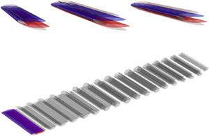
The spatial distribution of the streamwise velocity  $U$ computed with the SFD technique is depicted in figure 3 for the NACA 4412 periodic unswept wing at an angle of attack of $20^{\circ }$ and a Reynolds number ${\textit {Re}}=180$.

Figure 3. Base flow of the periodic unswept wing: spatial distribution of the streamwise velocity  $U$ in the spanwise plane $z=0$ ( $L_z = 8$) for $\alpha =20^{\circ }$ and ${\textit {Re}}=180$. The white solid lines represent the streamlines and the single blue one is the locus of the points where the streamwise velocity of the base flow is zero, i.e. the recirculation bubble region.
Laminar boundary layer separation occurs on the suction side of the wing. After the flow acceleration, as shown by the approaching of streamlines, in the proximity of the leading edge, the laminar boundary layer separates from the wing surface near  $x/c=0.35$ and reattaches slightly upstream of the trailing edge. Downstream of the separation and reattachment lines, two spanwise-homogeneous shear layers detach from the wing surface, delimiting an asymmetric recirculation bubble (blue solid line in figure 3) whose streamwise extent (measured from the leading edge) is $x/c = 1.84$. The length of the recirculation region is here identified using isolines of zero streamwise velocity. In addition, the morphology of an airfoil entails an asymmetry in the spanwise vorticity, with larger values near the leading edge with respect to those at the trailing edge. The length of the recirculation bubble varies as the angle of attack $\alpha$ and the Reynolds number ${\textit {Re}}$ change and, as discussed later in § 3.1, it drives the longitudinal wavenumber $k_{x_{\varLambda }}$ of the von Kármán mode.
Figure 4, displaying the streamwise and spanwise velocity components, illustrates the effect of the sweep angle  $\varLambda$ on the base flow for ${\textit {Re}}=400$ and the same angle of attack $\alpha$ as in figure 3, (i.e. for $\alpha =20^{\circ }$).

Figure 4. Base flow of the periodic  $25^{\circ }$ swept wing: spatial distribution of (a) the streamwise component $U$ and (b) the spanwise component $W$ of the velocity field in the spanwise plane $z=0$ for $\alpha =20^{\circ }$ and ${\textit {Re}}=400$. The white solid lines represent the corresponding velocity profiles at the streamwise locations $x/c=1.25$, $2$,
$2$,  $2.75$, $3.5$, $4.25$ and $5$, while the dashed ones refer to the unswept wing at the same flow conditions.
Figure 4(a) shows that the streamwise velocity depletion in the wake is attenuated by the sweep angle since the velocity deviation for  $\varLambda =25^{\circ }$ is lower with respect to the $\varLambda =0^{\circ }$ case and, consequently, the corresponding shear layer is slightly smoothed. This results in a reduction of the drag coefficient for the base flow (see figure 2). Increasing the Reynolds number leads to an increase of the recirculation bubble length, and a similar tendency can be observed by fixing the Reynolds number and increasing the angle of attack. As illustrated in figure 4(b), a non-zero sweep angle entails a non-zero spanwise component $W$, homogeneously distributed along the sweep angle direction and varying in the $x$–
$x$– $y$ plane, and as a consequence the three-dimensionalisation of the boundary layer. The spanwise flow is predominant in the recirculation bubble region and its mean value increases with the sweep angle.
We should stress that, since the geometry and the steady unforced base flow are invariant in the  $z_{\varLambda }$ direction (i.e. the sweep direction, see figure 1b), an alternative method to compute eigenmodes and the corresponding sensitivity could consist in using a change of variable to compute a two-dimensional base flow with three velocity components (2D-3C),
 \begin{equation} (\boldsymbol{U},P)(\boldsymbol{x}_{\varLambda})= (U,V,W,P)(x_{\varLambda},y_{\varLambda}) \quad\text{with } \frac{\partial (\,{\cdot}\,)}{\partial z_{\varLambda}} = 0, \end{equation}
and then introducing a decomposition into biglobal eigenmodes for the stability analysis, as follows:
 \begin{equation} (u',v',w',p')(\boldsymbol{x}_{\varLambda},t)= (\hat{u},\hat{v},\hat{w},\hat{p})(x_{\varLambda},y_{\varLambda}) \exp({\text{i}}k_{z_{\varLambda}}z_{\varLambda} + \sigma t) + \text{c.c.}, \end{equation}
where  $k_{z_{\varLambda }}$ is the spanwise wavenumber, $\sigma$ represents the complex temporal eigenfrequency and c.c. stands for the complex conjugate. In addition to saving computation cost, such a method can allow one to investigate a set of continuous values for the spanwise wavenumber whose values are subordinated to the choice of the spanwise extent $L_z$ in a fully three-dimensional approach, as can be noted by the discrete number of eigenvalues $\sigma _j$ in our spectra.
2.3. Direct and adjoint linear stability analyses
The dynamics of an infinitesimal perturbation  $\boldsymbol {q}^{\prime }(\boldsymbol {x}, t) = (\boldsymbol {u}^{\prime }, p^{\prime })^{\rm T}$ evolving on top of the base-flow solutions $\boldsymbol {Q}(\boldsymbol {x}) = (\boldsymbol {U}, P)^{\rm T}$ such as those described in § 2.2 is dictated by the linearised Navier–Stokes equations
 $$\begin{gather} \boldsymbol{\nabla} \boldsymbol{\cdot} \boldsymbol{u}^{\prime} = 0, \end{gather}$$
 $$\begin{gather}\frac{\partial \boldsymbol{u}^{\prime}}{\partial t} ={-} (\boldsymbol{U} \boldsymbol{\cdot} \boldsymbol{\nabla}) \boldsymbol{u}^{\prime} - (\boldsymbol{u}^{\prime} \boldsymbol{\cdot} \boldsymbol{\nabla}) \boldsymbol{U} - \boldsymbol{\nabla} p^{\prime} + \dfrac{1}{{\textit{Re}}} \boldsymbol{\Delta} \boldsymbol{u}^{\prime}. \end{gather}$$
In the frame of modal stability analysis, the disturbances are sought under the following form:
 \begin{equation} (u',v',w',p')(\boldsymbol{x},t)= (\hat{u},\hat{v},\hat{w},\hat{p})(\boldsymbol{x}) \exp(\sigma t) + \text{c.c.}, \end{equation}
where  $\sigma = \lambda + \mathrm {i} \omega$ is the complex eigenvalue, with $\lambda$ being the growth rate and $\omega$ the angular frequency, i.e. the frequency $f=\omega /2{\rm \pi}$. Substituting the normal-mode ansatz (2.7) into the linearised Navier–Stokes equations (2.6), the above linear initial-value problem can be recast as the following generalised eigenvalue problem:
 $$\begin{gather} \boldsymbol{\nabla} \boldsymbol{\cdot} \hat{\boldsymbol{u}} = 0, \end{gather}$$
 $$\begin{gather}\sigma \hat{\boldsymbol{u}} ={-} (\boldsymbol{U} \boldsymbol{\cdot} \boldsymbol{\nabla}) \hat{\boldsymbol{u}} - (\hat{\boldsymbol{u}} \boldsymbol{\cdot} \boldsymbol{\nabla}) \boldsymbol{U} - \boldsymbol{\nabla} \hat{p} + \dfrac{1}{{\textit{Re}}} \boldsymbol{\Delta} \hat{\boldsymbol{u}}. \end{gather}$$
The associated boundary conditions consist of the Dirichlet condition  $\hat {\boldsymbol {u}}=\boldsymbol {0}$ at the inlet $\varSigma _i$, and the remaining boundary conditions are the same as for the Navier–Stokes equations. The asymptotic temporal features of the perturbation are thus obtained from the least damped/most unstable eigenvalue. For instance, the imaginary part of the leading eigenvalue determines whether the fixed point experiences a pitchfork or transcritical ( $\omega =0$) or Hopf-type ( $\omega \neq 0$) bifurcation. Moreover, if this leading eigenvalue has a positive real part, i.e. $\lambda > 0$, the amplitude of the associated eigenmode will grow exponentially fast in time and, consequently, the base flow is asymptotically unstable. On the other hand, if the real part of all eigenvalues is negative (that is, for $\lambda _j < 0$ for all $j$ with $j$ the index of eigenvalues), the base flow is asymptotically stable and all eigenmodes will decay asymptotically in time.
Table 2 summarises the growth rate and the angular frequency of the most unstable mode obtained from the M1 and M2 meshes and two different polynomial orders on the M2 grid for an unswept wing at  $\alpha =20^{\circ }$ and ${\textit {Re}}=400$. As advocated in § 2.1, the two mesh resolutions provide comparable results, as the relative error is of the order of $0.1\,\%$. The analysis of the polynomial order on the M2 grid shows that the numerical convergence is substantially reached since, in this case, the relative error is of the order of $0.001\,\%$.
Table 2. Growth rate  $\lambda$ and angular frequency $\omega$ of the most unstable mode developing on an unswept wing with $L_z=8$ at $\alpha =20^{\circ }$ and ${\textit {Re}}=400$; the corresponding relative error $\varepsilon$ for (left) the M1 and M2 grids and (right) two polynomial orders $P$ on the M2 grid are also shown.

From a linear algebra point of view, the generalised eigenvalue problem (2.8) can be written as
 \begin{equation} \sigma \boldsymbol{\mathsf{B}} \,\hat{\boldsymbol{q}} = \boldsymbol{\mathsf{L}} \,\hat{\boldsymbol{q}}, \end{equation}
where  $\boldsymbol{\mathsf{B}}$ is a singular mass matrix enforcing that the velocity is an actual degree of freedom of the problem while the perturbation pressure field can be understood as a Lagrange multiplier to enforce the divergence-free constraint. The operator $\boldsymbol{\mathsf{L}}$ then corresponds to the Jacobian of the Navier–Stokes equations. Introducing a spatial inner product between two arbitrary state vectors $\boldsymbol {q}_1$ and $\boldsymbol {q}_2$, i.e.
 \begin{equation} \langle \boldsymbol{q}_1 \vert \boldsymbol{q}_2 \rangle = \int_{\varOmega} \boldsymbol{q}^* _1 \boldsymbol{\mathsf{B}} \,\boldsymbol{q}_2 \, \mathrm{d} \varOmega, \end{equation}
where  $\varOmega$ is the flow domain and the $^*$ stands for the complex conjugate, one can introduce the so-called ‘adjoint Navier–Stokes operator’ (Hill Reference Hill1995) satisfying
 \begin{equation} \langle \boldsymbol{q}_1 \vert \boldsymbol{\mathsf{L}} \,\boldsymbol{q}_2 \rangle = \langle\boldsymbol{\mathsf{L}}^{{{\dagger}}} \boldsymbol{q}_1 \vert \boldsymbol{q}_2 \rangle. \end{equation}
The corresponding adjoint eigenproblem then reads
 $$\begin{gather} \boldsymbol{\nabla} \boldsymbol{\cdot} \hat{\boldsymbol{u}}^{{{\dagger}}} = 0, \end{gather}$$
 $$\begin{gather}\sigma^* \hat{\boldsymbol{u}}^{{{\dagger}}} = (\boldsymbol{U} \boldsymbol{\cdot} \boldsymbol{\nabla})\hat{\boldsymbol{u}}^{{{\dagger}}} - \hat{\boldsymbol{u}}^{{{\dagger}}} \boldsymbol{\cdot} (\boldsymbol{\nabla} \boldsymbol{U})^{\rm T} + \boldsymbol{\nabla} \hat{p}^{{{\dagger}}} + \dfrac{1}{{\textit{Re}}} \boldsymbol{\Delta} \hat{\boldsymbol{u}}^{{{\dagger}}}, \end{gather}$$
where  $\boldsymbol {q}^{{\dagger} } (\boldsymbol {x}, t) =(\boldsymbol {u}^{{\dagger} },p^{{\dagger} })^{\rm T}=(\hat {u}^{{\dagger} }, \hat {v}^{{\dagger} }, \hat {w}^{{\dagger} },\hat {p}^{{\dagger} })^{\rm T} (\boldsymbol {x}) \exp (\sigma ^* t) + \text {c.c.}$ is the adjoint state vector. Note that the biorthogonality condition is used to normalise the adjoint:
 \begin{equation} \langle \hat{\boldsymbol{u}}^{{{\dagger}}} \vert \hat{\boldsymbol{u}} \rangle = 1. \end{equation}
For a discussion about the boundary conditions for the adjoint operator, interested readers are referred to Barkley et al. (Reference Barkley, Blackburn and Sherwin2008). While the notion of adjoint originated in optimisation theory, it has subsequently been widely applied in the hydrodynamics community to analyse linear and nonlinear transient growth of disturbances (Farrell Reference Farrell1988; Hill Reference Hill1995; Barkley et al. Reference Barkley, Blackburn and Sherwin2008). According to Marquet et al. (Reference Marquet, Sipp and Jacquin2008b), the adjoint can be used to identify the most stabilising or destabilising base-flow modification, or to map the sensitivity of leading modes to the application of an external force.
2.4. Sensitivity analysis of global modes
The sensitivity analysis consists in assessing how a variable is modified by the variation of a physical quantity. In particular, this study focuses on the sensitivity of the leading global modes. In this regard, a first instrument of the sensitivity analysis is the determination of the wavemaker region, i.e. the so-called structural sensitivity first introduced by Giannetti & Luchini (Reference Giannetti and Luchini2007) in the framework of global stability. The wavemaker is defined by the following relation:
 \begin{equation} \zeta(\boldsymbol{x}) = \frac{\Vert \hat{\boldsymbol{u}} \Vert \Vert \hat{\boldsymbol{u}}^{{{\dagger}}}\Vert} {\langle \hat{\boldsymbol{u}}^{{{\dagger}}} \vert \hat{\boldsymbol{u}} \rangle}, \end{equation}
where  $\Vert {\,{\cdot }\,} \Vert$ should be understood as the pointwise norm of the mode. It allows for identification of regions of the flow where generic structural modifications of the linearised Navier–Stokes operator lead to the strongest drift of the leading eigenvalue (see Appendix B).
The sensitivity of a given eigenvalue to an arbitrary base-flow modification or to a force can be considered. The concept of sensitivity to a base-flow modification was originally introduced by Bottaro, Corbett & Luchini (Reference Bottaro, Corbett and Luchini2003) in a local framework and later extended to the global framework also for a body force by Marquet et al. (Reference Marquet, Sipp and Jacquin2008b). The variations  $\delta \sigma$ of the complex eigenvalue with respect to an arbitrary small-amplitude base-flow modification $\delta \boldsymbol {U}$ can be formally related through the inner-product definition:
 \begin{equation} \delta \sigma = \langle \boldsymbol{\nabla}_{\boldsymbol{U}} \sigma \vert \delta\boldsymbol{U}\rangle . \end{equation}
The specific form of the sensitivity  $\boldsymbol {\nabla }_{\boldsymbol {U}} \sigma$ is derived by a Lagrangian-based approach (see appendix A in Marquet et al. (Reference Marquet, Sipp and Jacquin2008b) for a complete derivation) and reads
 \begin{equation} \boldsymbol{\nabla}_{\boldsymbol{U}} \sigma ={-} ( \boldsymbol{\nabla} \hat{\boldsymbol{u}})^{\rm H} \boldsymbol{\cdot} \hat{\boldsymbol{u}}^{{{\dagger}}} + \boldsymbol{\nabla}\hat{\boldsymbol{u}}^{{{\dagger}}} \boldsymbol{\cdot} \hat{\boldsymbol{u}}^*, \end{equation}
where the superscript H denotes the transconjugate. Note that  $\boldsymbol {\nabla }_{\boldsymbol {U}} \sigma$ is a complex vector field, and that variations of the growth rate $\delta \lambda$ and frequency $\delta \omega$ are linked to $\delta \sigma$ via $\boldsymbol {\nabla }_{\boldsymbol {U}} \lambda =\mathrm {Re}(\boldsymbol {\nabla }_{\boldsymbol {U}} \sigma )$ and $\boldsymbol {\nabla }_{\boldsymbol {U}} \omega =-\mathrm {Im}(\boldsymbol {\nabla }_{\boldsymbol {U}} \sigma )$. It should be stressed that the base-flow modification $\delta \boldsymbol {U}$ is generic since $\boldsymbol {U} + \delta \boldsymbol {U}$ is not assumed to be a steady solution of the equations governing the base flow.
Analogously, the sensitivity to a force can be derived. Variations of a particular eigenvalue  $\delta \sigma$ induced by infinitesimal variations $\delta \boldsymbol {F}$ of the body force are formally described by the following relation:
 \begin{equation} \delta \sigma = \langle \boldsymbol{\nabla}_{\boldsymbol{F}} \sigma \vert \delta \boldsymbol{F} \rangle, \end{equation}
where  $\boldsymbol {\nabla }_{\boldsymbol {F}} \sigma$ defines the sensitivity to a steady force modification. As for the base-flow sensitivity, $\boldsymbol {\nabla }_{\boldsymbol {F}} \sigma$ is a complex vector field so that $\boldsymbol {\nabla }_{\boldsymbol {F}} \lambda =\mathrm {Re}(\boldsymbol {\nabla }_{\boldsymbol {F}} \sigma )$ and $\boldsymbol {\nabla }_{\boldsymbol {F}} \omega =-\mathrm {Im}(\boldsymbol {\nabla }_{\boldsymbol {F}} \sigma )$. The Lagrangian-based approach allows the following expression to be derived for the force sensitivity:
 \begin{equation} \boldsymbol{\nabla}_{\boldsymbol{F}} \sigma = \boldsymbol{U}^{{{\dagger}}}, \end{equation}
where  $\boldsymbol {Q}^{{\dagger} } = (\boldsymbol {U}^{{\dagger} },P^{{\dagger} })^{\rm T}$ is the adjoint (complex) base flow whose governing equations read
 $$\begin{gather} \boldsymbol{\nabla} \boldsymbol{\cdot} \boldsymbol{U}^{{{\dagger}}} = 0, \end{gather}$$
 $$\begin{gather}- (\boldsymbol{U} \boldsymbol{\cdot} \boldsymbol{\nabla}) \boldsymbol{U}^{{{\dagger}}} + \boldsymbol{U}^{{{\dagger}}} \boldsymbol{\cdot} (\boldsymbol{\nabla} \boldsymbol{U})^{\rm T} - \boldsymbol{\nabla} P^{{{\dagger}}} - \dfrac{1}{{\textit{Re}}} \boldsymbol{\Delta} \boldsymbol{U}^{{{\dagger}}} = \boldsymbol{\nabla}_{\boldsymbol{U}} \sigma, \end{gather}$$
with  $\boldsymbol {U}^{{\dagger} }=\boldsymbol {0}$ at the inlet and on the wing walls, symmetrical conditions on the lower and upper boundaries, and periodic conditions on the lateral boundaries. Note that computing the force sensitivity $\boldsymbol {\nabla }_{\boldsymbol {F}} \sigma$, which is the focus of § 3.3, requires the computation of the base-flow sensitivity function beforehand.
3. Global stability and sensitivity analyses of leading global modes
3.1. Global stability analysis over unswept periodic wings
We first consider the global stability analysis of the massively separated flow around a NACA 4412 periodic unswept wing at  $\alpha =20^{\circ }$ and ${\textit {Re}}=400$. Figure 5 shows the corresponding eigenspectrum and some direct global eigenmodes. Following the notation in figure 5(a), there are depicted the real parts of the streamwise velocity $\mathrm {Re}(\hat {u})$ of the eigenfunction corresponding to the two-dimensional von Kármán mode $\sigma _{1_{\varLambda _{0}}}$ (figure 5b), the three-dimensional von Kármán mode $\sigma _{2_{\varLambda _{0}}}$ (figure 5c) and the three-dimensional centrifugal mode $\sigma _{8_{\varLambda _{0}}}$ (figure 5d) (Theofilis, Hein & Dallmann Reference Theofilis, Hein and Dallmann2000; Kitsios et al. Reference Kitsios, Rodríguez, Theofilis, Ooi and Soria2009; Rodríguez & Theofilis Reference Rodríguez and Theofilis2011).

Figure 5. Global stability results and direct global eigenmodes. (a) Eigenspectrum of the flow around a periodic unswept wing with a span extent of  $L_z=8$ at $\alpha =20^{\circ }$ and ${\textit {Re}}=400$. The double circle symbol indicates that the algebraic multiplicity of the corresponding eigenvalue is two. Only the positive-frequency part of the eigenspectrum is shown. The eigenvalues are ordered following the notation $\sigma _{j_{\varLambda _{i}}}$, where $j$ follows an order relation with respect to the growth rate such that $\sigma _1$ represents the least stable eigenvalue and $i$ denotes the value of the sweep angle $\varLambda$. (b–d) According to this notation, depicted are the real parts of the streamwise velocity $\mathrm {Re}(\hat {u})$ of the eigenfunction corresponding to (b) the two-dimensional von Kármán mode $\sigma _{1_{\varLambda _{0}}}$, (c) the three-dimensional von Kármán mode $\sigma _{2_{\varLambda _{0}}} \equiv \sigma _{3_{\varLambda _{0}}}$ with $k_{z_{\varLambda }}= \pm {\rm \pi}/4$ and (d) the three-dimensional centrifugal mode $\sigma _{8_{\varLambda _{0}}}$ with $k_{z_{\varLambda }}= \pm 3{\rm \pi} /4$. Red (blue) contours correspond to positive (negative) values of 10 % of the maximal absolute value of $\mathrm {Re}(\hat {u})$. These conventions hold throughout the paper.
Here the spanwise extent is set to  $L_z=8$, and three-dimensional modes are selected for wavenumbers defined as $k_{z_{\varLambda }}=2 {\rm \pi}n/L_z$, with $n \in \mathbb {Z}$ in order to satisfy periodicity on the lateral boundaries. Continuous eigenbranches are therefore discretised as a function of $L_z$. This is the case for both the von Kármán and three-dimensional centrifugal modes.
As illustrated in figure 5(c), the von Kármán mode is characterised by a spanwise wavenumber  $k_{z_{\varLambda }} = \pm {\rm \pi}/4$, whereas the three-dimensional centrifugal mode shown in figure 5(d) has a wavenumber $k_{z_{\varLambda }} = \pm 3{\rm \pi} /4$. The plus or minus sign corresponds to the superposition of two invariant modes with respect to the phase velocity in the positive or negative spanwise direction. This justifies the double algebraic multiplicity of all the eigenvalues (except the two-dimensional von Kármán mode) in the spectrum of figure 5(a). As a result, when $\varLambda =0^\circ$, $\sigma _{2_{\varLambda _{0}}} \equiv \sigma _{3_{\varLambda _{0}}}$ with $\vert k_{z_{\varLambda }} \vert = {\rm \pi}/4$. In the spectrum in figure 5(a), other three-dimensional von Kármán modes have been indicated. They present a spatial distribution similar to the global mode in figure 5(c) but present increasing spanwise wavenumber. In particular, the modes $\sigma _{4_{\varLambda _{0}}}$ and $\sigma _{5_{\varLambda _{0}}}$ are characterised by $\vert k_{z_{\varLambda }} \vert = {\rm \pi}/2$, whereas the modes $\sigma _{6_{\varLambda _{0}}}$ and $\sigma _{7_{\varLambda _{0}}}$ are characterised by $\vert k_{z_{\varLambda }} \vert = 3{\rm \pi} /4$ (see also the red curves in figure 11).
In fact, regardless of the spanwise wavenumber's sign, three-dimensional modes (both the von Kármán and centrifugal types) with the same spanwise wavenumber (in absolute value) ought to have the same stability properties (i.e. equal growth rates and frequencies). The spanwise wavenumber of the two-dimensional von Kármán mode is null, i.e.  $k_{z_{\varLambda }}=0$, and its algebraic multiplicity is unity. It represents the most unstable global mode with a frequency of $0.338$. The difference between the nonlinear natural frequency (see table 1) and that obtained with the linear stability analysis is attributable to the distortion due to the nonlinear effects (Barkley Reference Barkley2006; Sipp & Lebedev Reference Sipp and Lebedev2007). It should be noted that this analysis is carried out far beyond the bifurcation threshold since the growth rate value is $\lambda = 0.411$, as shown in figure 5(a) (see also table 2).
Varying the Reynolds number  ${\textit {Re}}$ and the angle of attack $\alpha$, the marginal stability curves were computed as a function of ${\textit {Re}}$ for the leading mode. The results are collected in figure 6, together with the thresholds for the leading three-dimensional centrifugal mode and the corresponding Strouhal numbers.

Figure 6. Marginal curves in  $\log$– $\log$ plots for the flow around a periodic unswept wing: (a) the emergence threshold of the two-dimensional von Kármán mode together with that of the three-dimensional centrifugal mode in the $\alpha \unicode{x2013}{\textit {Re}}$ plane; (b) the critical Strouhal number of the von Kármán mode; and (c) the spanwise wavenumber $k_{z_{\varLambda }}$ of the leading three-dimensional centrifugal mode as a function of the angle of attack.
As observed also by He et al. (Reference He, Gioria, Pérez and Theofilis2017) for the NACA 0009, 0015 and 4415, the leading flow eigenmode is the two-dimensional von Kármán mode and not the stationary three-dimensional mode, whose emergence threshold is higher, i.e.  ${\textit {Re}}^{{\tiny {3DC}}} _{{cr}}(\alpha ) > {\textit {Re}}^{{\tiny {VK}}} _{{cr}}(\alpha ), \forall \alpha \in [0;{\rm \pi} /2]$ ${\textit {Re}}^{3DC}_{cr}(\alpha ) > {\textit {Re}}^{VK}_{cr}(\alpha )$, for all $\alpha \in [0;{\rm \pi} /2]$ (see figure 6a).
Figure 7 shows the Reynolds number at which the three-dimensional centrifugal mode becomes marginally stable as a function of that concerning the two-dimensional von Kármán mode.

Figure 7. Relation between the critical Reynolds number of the leading three-dimensional centrifugal mode and that of the two-dimensional von Kármán mode.
As also confirmed by direct numerical simulations, we conclude that this stationary three-dimensional mode (as well as the three-dimensional von Kármán modes) does not contribute to the dynamics of unswept wings at low Reynolds numbers. The critical Strouhal number of the two-dimensional von Kármán mode decreases as the angle of attack increases (see figure 6b), with  $d=c \sin \alpha$, which corresponds to the vertical distance between the leading and trailing edges or the characteristic length scale for the interactions of shear layers across the wake (see figure 23b in Appendix A). The spanwise wavenumber of the leading three-dimensional centrifugal mode $k_{z_{\varLambda }} ^{{{3DC}}}$ as a function of the angle of attack is reported in figure 6(c) and is also depicted in figure 8. It should be noted that all quantities, ${\textit {Re}}_{{cr}}$, $St_{{cr}}$ and $k_{z_{\varLambda }} ^{{{3DC}}}$, follow power laws with respect to the angle of attack.

Figure 8. Growth rate  $\lambda$ of leading global modes as a function of the spanwise wavenumber $k_{z_{\varLambda }}$ for four different angles of attack, $\alpha =10^{\circ }$, $20^{\circ }$, $32^{\circ }$ and $50^{\circ }$, at the respective Reynolds numbers at which the leading three-dimensional centrifugal mode becomes marginally stable. The solid (dashed) lines refer to the von Kármán (three-dimensional centrifugal) modes. The corresponding spanwise wavenumbers $k_{z_{\varLambda }} ^{3DC}$ are collected in figure 6(c).
Figure 8 shows the growth rate  $\lambda$ of the leading global modes with respect to the spanwise wavenumber $k_{z_{\varLambda }}$ for four different angles of attack, $\alpha =10^{\circ }$, $20^{\circ }$, $32^{\circ }$ and $50^{\circ }$, at the respective Reynolds numbers for which the leading three-dimensional centrifugal mode is marginally stable (see also figure 4b in Nastro et al. (Reference Nastro, Robinet, Loiseau, Passaggia, Baldas, Mazellier and Stefes2022b)). As far as the von Kármán modes are concerned (see the solid lines), the growth rate decreases with a parabolic behaviour for increasing spanwise wavenumber. Interestingly, the eigenbranch of von Kármán modes crosses the marginal stability axis at a spanwise wavenumber close to the leading three-dimensional centrifugal mode (see the dashed lines). However, no clear explanation can justify this observation.
Since the flow dynamics are driven by the two-dimensional von Kármán mode, we now analyse some of its properties with respect to the respective base flow at the critical conditions. Figure 9(a) shows the largest streamwise extent of the recirculation bubble  $x_{{rb}}/c$ and the streamwise location of the separation line $x_{{sep}}/c$ computed on the base flows corresponding to the critical conditions ${\textit {Re}}_{{cr}}$.

Figure 9. (a) For each critical point  ${\textit {Re}}_{{cr}}$, the maximal streamwise extent of the recirculation bubble (left $y$-axis and red line) and the streamwise location of the separation line (right $y$-axis and blue line), both evaluated on the corresponding base flows. (b) Streamwise wavenumber of the two-dimensional von Kármán mode obtained by fast Fourier transform of the velocity spatial signal as a function of the critical angle of attack. (c) Critical Strouhal number as a function of the streamwise wavenumber $k_{x_{\varLambda }}$.
As the critical Reynolds number decreases and, consequently, the critical angle of attack increases, the recirculation bubble becomes larger and the laminar boundary layer separation is located farther upstream, ranging from  $x_{{sep}}/c = 0.6$ for ${\textit {Re}}_{{cr}} = 1046$ and $\alpha _{{cr}} = 5^{\circ }$ to a leading-edge separation ( $x_{{sep}}/c = 0.03$) for ${\textit {Re}}_{{cr}} = 32.9$ and $\alpha _{{cr}} = 80^{\circ }$.
Figure 9(b) illustrates the streamwise wavenumber  $k_{x_{\varLambda }}$ of the two-dimensional von Kármán mode obtained by fast Fourier transform of the eigenmode velocity spatial signal as a function of the critical angle of attack. The streamwise wavelength of the leading eigenmode increases for higher critical angles of attack as a result of the thickening of the recirculation region. The characteristic length scale of the recirculation region thus drives the eigenmode wavelength. As a consequence, the streamwise wavenumber decreases monotonically when increasing the angle of attack and follows a power law, which is similar to that obtained for the critical Strouhal number and decreases with $d=c \sin \alpha$ measuring the interaction distance between the shear layers – compare figure 9(b) with figures 6(c,d) and see figure 23(b) in Appendix A. Evidently, these two length scales, $x_{{rb}}/c$ and $d$, are tied, since they increase and decrease proportionally if one moves along the marginal curve in the $\alpha \unicode{x2013}{\textit {Re}}$ plane. Whence, the eigenmode frequency is linearly proportional to the streamwise wavenumber, leading to a constant critical phase velocity $c_{x_{\varLambda }} \approx 0.93$.
3.2. Influence of sweep angle on global modes
In this section, we discuss the effect of the sweep angle  $\varLambda$ on the leading global modes developing around periodic NACA 4412 wings. We first consider the same conditions as in figure 5 to elucidate the influence of the sweep angle on a larger set of unstable or weakly stable global modes.
Figure 10 shows the spectrum for three different sweep angles and some direct global eigenmodes for the specific case of  $\varLambda = 25^{\circ }$.

Figure 10. Global stability results and direct global eigenmodes. (a) Eigenspectrum for  $\varLambda =0^{\circ },\ 12^{\circ },\ 25^{\circ }$ at $\alpha =20^{\circ }$ and ${\textit {Re}}=400$. (b–e) According to spectrum notation, depicted for the $\varLambda =25^{\circ }$ case are the real parts of the streamwise velocity $\mathrm {Re}(\hat {u})$ of the eigenfunction corresponding to (b) the two-dimensional von Kármán mode $\sigma _{1_{\varLambda _{25}}}$, the three-dimensional von Kármán modes (c) $\sigma _{2_{\varLambda _{25}}}$ with $k_{z_{\varLambda }}={\rm \pi} /4$ and (d) $\sigma _{3_{\varLambda _{25}}}$ with $k_{z_{\varLambda }}= - {\rm \pi}/4$ and (e) the three-dimensional centrifugal mode $\sigma _{8_{\varLambda _{25}}}$ characterised by $k_{z_{\varLambda }}=3{\rm \pi} /4$.
As we increase the sweep angle, both the frequency and the growth rate of all leading global modes undergo a slight reduction. This suggests that instabilities are attenuated over spanwise-periodic wings for increasing  $\varLambda$. As observed for the unswept wing, the two-dimensional von Kármán mode (depicted in figure 10b for $\varLambda =25^{\circ }$) remains the most unstable global mode with $f=0.329$ and $0.300$ for $\varLambda =12^{\circ }$ and $25^{\circ }$, respectively. The three-dimensional eigenmodes, both the von Kármán and three-dimensional centrifugal ones, do not take part in the dynamics of swept wings in this Reynolds number regime, as proved by direct numerical simulations. It is worth noting that introducing a non-zero sweep angle leads to a split in the three-dimensional von Kármán modes having the same spanwise wavenumber in absolute value. In fact, as a non-zero sweep angle induces a sideward deflection (sidewash) of the free stream (see figure 4b), the spanwise direction is no longer invariant with respect to mode displacements in the positive or negative direction. Global modes now display a unitary algebraic multiplicity as opposed to the $\varLambda =0^{\circ }$ case. Keeping the wavenumber $k_{z_{\varLambda }}$ constant in absolute value, the frequency decreases for the corresponding negative value and increases for the positive one due to the Doppler effect. Analogously, the growth rate is lower in the former and higher in the latter case.
Considering three-dimensional von Kármán modes  $\sigma _{2_{\varLambda _{25}}}$ illustrated in figure 10(c) and $\sigma _{3_{\varLambda _{25}}}$ in figure 10(d), the former is characterised by a spanwise wavenumber $k_{z_{\varLambda }} = {\rm \pi}/4$, whereas the latter has $k_{z_{\varLambda }} = - {\rm \pi}/4$. As a consequence, $\sigma _{2_{\varLambda _{25}}}$ moves in the same direction induced by the sidewash, whereas $\sigma _{3_{\varLambda _{25}}}$ moves against the side stream. In addition, the introduction of a sweep angle causes the three-dimensional centrifugal modes to detach from the zero-frequency axis. Figure 10(e) illustrates the most unstable three-dimensional centrifugal mode for $\varLambda =25^{\circ }$, $\sigma _{8_{\varLambda _{25}}}\!$, which is characterised by a spanwise wavenumber $k_{z_{\varLambda }} = 3{\rm \pi} /4$. For a fixed non-zero sweep angle, they present a range of low frequencies which substantially increase as $\varLambda$ increases, whereas the growth rates are subjected to a slight attenuation. They present only positive values of the spanwise wavenumber and as a consequence move only along the positive spanwise direction following the mean side stream.
Let us consider in more detail the influence of the sweep angle on the wave properties of the global eigenmodes depicted in figure 10. It should be remembered that it is also possible to define the wave angle as  $\phi =\tan ^{-1}(k_{z_{\varLambda }}/k_{x_{\varLambda }})$. The main features of the global eigenmodes for a $25^{\circ }$ swept periodic wing flow at $\alpha =20^{\circ }$ and ${\textit {Re}}=400$ are summarised in table 3 or von Kármán modes and in table 4 for three-dimensional centrifugal modes and compared to the $\varLambda =0^{\circ }$ and $12^{\circ }$ cases in figure 11.
Table 3. Main features of the von Kármán modes for  $\varLambda =25^{\circ }$: streamwise wavenumber $k_{z_{\varLambda }}$, wave angle $\phi$, growth rate $\lambda$ and frequency $f$.
$f$.


Figure 11. Influence of the sweep angle on the wave properties of the global eigenvalues: (a) growth rate  $\lambda$, (b) frequency $f$, (c) phase velocity $c_{z_{\varLambda }}$ and (d) group velocity $v_{z_{\varLambda }}$ as functions of the spanwise wavenumber $k_{z_{\varLambda }}$ at $\alpha =20^{\circ }$ and ${\textit {Re}}=400$ for $\varLambda =0^{\circ },\ 12^{\circ },\ 25^{\circ }$.
Table 4. Main features of the three-dimensional centrifugal modes for  $\varLambda =25^{\circ }$: streamwise wavenumber $k_{z_{\varLambda }}$, wave angle $\phi$, growth rate $\lambda$ and frequency $f$.
$f$.

Figure 11 shows the growth rate  $\lambda$, the frequency $f$, the spanwise phase velocity $c_{z_{\varLambda }}$ and the spanwise group velocity $v_{z_{\varLambda }}$ as functions of the spanwise wavenumber at $\alpha =20^{\circ }$ and ${\textit {Re}}=400$ for $\varLambda =0^{\circ },\ 12^{\circ },\ 25^{\circ }$. As done previously, figure 11 follows the convention of representing only the part of the eigenspectrum with positive frequencies. Increasing the sweep angle $\varLambda$ leads to a slight decrease of the growth rate. As far as the von Kármán modes are concerned, this decrease is more pronounced for negative spanwise wavenumbers, as discussed earlier. For all sweep angles considered here, the growth rates of both the von Kármán and three-dimensional centrifugal modes have a parabolic-like behaviour (see figure 11a).
As shown in figure 11(b), whilst the frequency of the three-dimensional centrifugal modes shows a linear trend and therefore a non-dispersive behaviour, that of the von Kármán modes has a weakly parabolic behaviour, suggesting a slight dispersion in the spanwise direction (Fraternale, Nastro & Tordella Reference Fraternale, Nastro and Tordella2021). Introducing a sweep angle induces a monotonic behaviour of the frequency curves with respect to the spanwise wavenumber. As far as the von Kármán modes are concerned, the curves rotate anticlockwise around the value corresponding to  $k_{z_{\varLambda }}=0$, providing a decrease for negative spanwise wavenumbers and an increases for positive ones because of the Doppler effect introduced by the sideward deflection of the free stream. The substantial difference between the phase and group velocities is indicative of the spanwise dispersion of the von Kármán modes, whereas for the three-dimensional centrifugal modes the phase velocity coincides with the group one, which is comparable to the base-flow sidewash (see figure 11c,d).
The adjoint global eigenmodes corresponding to the  $25^{\circ }$ swept periodic wing flow at $\alpha =20^{\circ }$ and ${\textit {Re}}=400$ are compared with those of the unswept wing flow in figure 12, with the same convention as in figures 5 and 10.

Figure 12. Comparison of the adjoint global eigenmodes for  $\varLambda =0^{\circ }$ and $25^{\circ }$: real parts of the streamwise velocity $\mathrm {Re}({\hat {u}^{{\dagger} }})$ of the eigenfunction corresponding to the two-dimensional von Kármán mode for (a) $\varLambda =0^{\circ }$ and (b) $\varLambda =25^{\circ }$, the three-dimensional von Kármán mode with $k_{z_{\varLambda }}={\rm \pi} /4$ for (c) $\varLambda =0^{\circ }$ and (d) $\varLambda =25^{\circ }$, the three-dimensional von Kármán mode with $k_{z_{\varLambda }}=-{\rm \pi} /4$ for (e) $\varLambda =0^{\circ }$ and (f) $\varLambda =25^{\circ }$ and the three-dimensional centrifugal mode with $k_{z_{\varLambda }}=3 {\rm \pi}/4$ for (g) $\varLambda =0^{\circ }$ and (h) $\varLambda =25^{\circ }$.
The streamwise velocities are concentrated around the wing surface and exhibit only weak spatial oscillations upstream from the wing (lower than  $10\,\%$ of the maximal absolute value, therefore not visible in figure 12). Varying the sweep angle $\varLambda$ does not yield substantial differences in the spatial distribution of the adjoint modes, at least for this flow regime. For a fixed angle of attack, increasing (respectively decreasing) the Reynolds number leads to a streamwise elongation (respectively approaching) of the sheet structures forming the adjoint modes, in agreement with the thickening (respectively shrinking) of the recirculation bubble region. The same observation applies for constant Reynolds numbers with an increase (respectively decrease) of the angle of attack $\alpha$.
Figure 13(a) shows the spectrum for different Reynolds numbers on a  $25^{\circ }$ swept wing at angle of attack of $20^{\circ }$. As done for the unswept case, the Reynolds number ${\textit {Re}}$ and the angle of attack $\alpha$ were varied, and the marginal stability for $\varLambda =12^{\circ }$ and $25^{\circ }$ was determined. The trend in the critical Reynolds number with respect to the sweep angle is collected in figure 13 together with the corresponding Strouhal numbers for $\alpha =10^{\circ }$, $20^{\circ }$ and $32^{\circ }$.

Figure 13. Marginal curves for the flow around periodic swept wings. (a) Spectrum of  $25^{\circ }$ swept wing at angle of attack of $20^{\circ }$ for several Reynolds numbers, with the solid line denoting the von Kármán modes and the dash-dotted one the three-dimensional centrifugal modes. (b–g) Critical Reynolds number as a function of the sweep angle for (b) $\alpha =10^{\circ }$, (d) $\alpha =20^{\circ }$ and (f) $\alpha =32^{\circ }$; and corresponding critical Strouhal number for the same angles of attack, (c) $\alpha =10^{\circ }$, (e) $\alpha =20^{\circ }$ and (g) $\alpha =32^{\circ }$.
For instance, for  $\varLambda =25^{\circ }$ and $\alpha =20^{\circ }$, the critical Reynolds number is found to be $188.8$ with a characteristic frequency of $0.310$, which coincides perfectly with that obtained from the direct numerical simulation. Considering a Reynolds number of $220$, the deviation between the nonlinear frequency and that obtained from the stability analysis remains less than $0.03\,\%$. Then it increases significantly for $Re=400$, where the frequency given by global stability analysis is $0.300$ and that from the nonlinear simulation is $0.442$. The critical Reynolds number increases, confirming the attenuation of the flow behaviour over spanwise-periodic wings for increasing $\varLambda$ (see figure 13b,d,f). In addition, increasing the wing sweep angle leads to a reduction of the critical frequency, as depicted in figure 13(c,e,g).
The remainder of the present work focuses on a sensitivity analysis (§ 3.3) and control of the unsteady wake (§ 3.5), and the analysis is restricted to  $\alpha =20^{\circ }$, which allows for understanding the fundamental characteristics of the wake forming in the flow of a stalled lifting body with a non-zero sweep angle. Moreover, the analysis is carried out in the vicinity of the critical Reynolds number of the first bifurcation to assure a stable von Kármán orbit.
3.3. Sensitivity analysis of the leading global mode
We are now interested in the stabilisation of the flow by means of a steady force that is assumed to modify only the base flow (Marquet et al. Reference Marquet, Sipp and Jacquin2008b). The angle of attack is kept constant at  $\alpha =20^{\circ }$ and we consider a Reynolds number equal to $190$, which is very close to the critical one ( $\vert {\textit {Re}} - {\textit {Re}}_{{cr}} \vert < 1.5$). For these flow conditions, the leading global mode developing on the $25^{\circ }$ swept periodic wing is depicted in figure 14 together with the corresponding adjoint mode.

Figure 14. Direct and adjoint leading global mode for  $\varLambda =25^{\circ }$, $\alpha =20^{\circ }$ and ${\textit {Re}}=190$: contours of the real part of the streamwise velocity of (a) the direct global mode and (e) the adjoint one. (b–d) Slices in the spanwise plane $z=0$ ( $L_z=8$) of (b) streamwise, (c) cross-stream and (d) spanwise velocity components for the direct mode, and (f–h) the same for the adjoint one, respectively.
It should be noted that, in the vicinity of the critical point, the direct global mode presents structure extending into the far wake, whereas, as the Reynolds number (or the angle of attack) increases, the global mode contracts, concentrating around the recirculation bubble, at whose closure point is approximately the maximum value of the mode energy. The break in the spatial symmetry of the mode developing on the wing can be noted in the spanwise component, whose lobe structures differ in shape, moving from above to below the wake. The adjoint global mode remains concentrated around the wing surface and exhibits weak spatial oscillations upstream from the wing.
The sensitivity analysis to a steady force, presented in § 2.4, is now applied to the leading global eigenvalue. It should be remembered that, thanks to the sensitivity analysis to a steady force, base-flow modifications induced by an arbitrary force  $\delta \boldsymbol {F}$ do not need to be explicitly computed in order to determine the eigenvalue variations $\delta \sigma$ (Marquet et al. Reference Marquet, Sipp and Jacquin2008b). The sensitivity function to a base-flow modification involved as source term in (2.19) for the determination of the sensitivity to a steady force is illustrated in Appendix C.
Figure 15 depicts the growth-rate sensitivity to a steady force  $\boldsymbol {\nabla }_{\boldsymbol {F}} \lambda$ of the leading eigenvalue $\sigma _{1_{\varLambda _{25}}}$ computed for the same conditions as in figure 14.

Figure 15. Spatial distribution in the plane  $z=0$ of the growth-rate sensitivity to a steady force of the leading eigenvalue for $\varLambda =25^{\circ }$, $\alpha =20^{\circ }$ and ${\textit {Re}}=190$: (a) streamwise, (b) cross-stream and (c) spanwise components of $\boldsymbol {\nabla }_{\boldsymbol {F}} \lambda$.
Figure 15(a) shows that a steady force acting inside the recirculation bubble in the positive streamwise direction is stabilising, since the growth-rate sensitivity exhibits negative values. Furthermore, an extended region localised on the suction side is stabilising as well. It represents a region of interest for the arrangement of jet actuators. Conversely, acting on the shear zones outside the recirculation region in the positive  $x$ direction induces a positive variation of the growth rate, i.e. $\delta \lambda > 0$. Regarding the cross-stream direction, figure 15(b) shows that the highest sensitivity is concentrated around the trailing edge with negative values and along the suction side with positive values. As far as the spanwise component is concerned, the most sensitive regions are the shear layers which host negative values of the growth-rate sensitivity such that a positive spanwise force has a stabilising effect, i.e. $\delta \lambda < 0$. As mentioned by Marquet et al. (Reference Marquet, Sipp and Jacquin2008b), the present approach would also be able to predict whether a distributed force or a non-local one has a stabilising or destabilising effect, although a local force has been adopted here to interpret the sensitivity maps.
The frequency sensitivity to a steady force is depicted in figure 16(a–c) in terms of streamwise, cross-stream and spanwise components, respectively. The streamwise component of the frequency sensitivity function shows that a stabilising local force (see figure 15a) is associated with an increase of the frequency in both the separation and recirculation regions, and a slight decrease in the outer region. Similarly to the growth-rate sensitivity function, the cross-stream component is essentially concentrated around the trailing edge, where a localised normal oscillator would yield an increase of the frequency. Analogously, in the near proximity of the leading edge, a local force would slightly increase the frequency, whereas in the extended region along the suction side, it would lead to a shift towards low frequencies. For the spanwise component, a local force along the positive  $z$ axis would provide a decrease of the frequency when acting on the suction side and around the trailing edge and a shift towards high frequencies when acting inside the recirculation bubble.

Figure 16. Spatial distribution in the plane  $z=0$ of the frequency sensitivity to a steady force of the leading eigenvalue for $\varLambda =25^{\circ }$, $\alpha =20^{\circ }$ and ${\textit {Re}}=190$: (a) streamwise, (b) cross-stream and (c) spanwise components of $\boldsymbol {\nabla }_{\boldsymbol {F}} \omega$.
We now consider a specific steady force  $\boldsymbol {F}$ modelling a small increment in the drag force. The effect of such a body force can be related to that of a small-diameter cylindrical rod, which would lead to a pointwise supply of momentum to the flow equal and opposite to the anticipated drag (Hill Reference Hill1992). This force is applied to the unforced base-flow solution of (2.3) with $\boldsymbol {F} = \boldsymbol {0}$ and is therefore denoted $\delta \boldsymbol {F}$ according to the general formalism described in § 2.4. In particular, it is considered to be proportional to the square of the base flow field (see also (5.1) in Marquet et al. (Reference Marquet, Sipp and Jacquin2008b)) according to the following relation:
 \begin{equation} \delta \boldsymbol{F} ={-} \epsilon \Vert \boldsymbol{U} \Vert \boldsymbol{U} \, \delta(x-x_{{c}}(z),y-y_{{c}}), \end{equation}
where  $\epsilon$ is the amplitude parameter and $(x_{{c}},y_{{c}})$ is the station where the control is applied. In order to apply the steady force homogeneously along the span, the streamwise coordinate for the control is found to be a function of the spanwise direction as follows: $x_{{c}}(z) = x_{{c}}(z=0) + z \tan \varLambda$.
In the case of cylinder flow, previous numerical studies (Hill Reference Hill1992; Marquet et al. Reference Marquet, Sipp and Jacquin2008b; Boujo Reference Boujo2021) have shown that a mathematical form like that of (3.1) models appropriately the effect of a cylindrical rod-type physical control device. Such a device can control the vortex shedding at low Reynolds number, as demonstrated experimentally by Strykowski & Sreenivasan (Reference Strykowski and Sreenivasan1990) and later via Navier–Stokes simulations by Dipankar, Sengupta & Talla (Reference Dipankar, Sengupta and Talla2007). However, we point out that the presence of a physical control device (such as a cylindrical rod) in the flow could be modelled by a force acting not only at the base-flow level (as considered here) but also at the perturbation level in order to take into account their respective effects on the flow stability and to gain a more detailed prediction of the stabilising/destabilising regions, as shown by Marquet et al. (Reference Marquet, Sipp, Chomaz and Jacquin2008a) for the passive control of cylinder flow. Using the force modelled by (3.1) and the relation (2.17), variations of the growth rate and frequency (normalised by the amplitude  $\epsilon$) can be expressed as follows:
 $$\begin{gather} \frac{\delta \lambda}{\epsilon} ={-} \Vert \boldsymbol{U} \Vert \boldsymbol{U} (\boldsymbol{\nabla}_{\boldsymbol{F}} \lambda \boldsymbol{\cdot} \boldsymbol{U}), \end{gather}$$
 $$\begin{gather}\frac{\delta \omega}{\epsilon} ={-} \Vert \boldsymbol{U} \Vert \boldsymbol{U} (\boldsymbol{\nabla}_{\boldsymbol{F}} \omega \boldsymbol{\cdot} \boldsymbol{U}). \end{gather}$$
 The quantities expressed by (3.2a) and (3.2b) are illustrated in figures 17(a) and 17(b), respectively. The results are shown in the plane  $z=0$ but they are homogeneous along the span because of the spanwise homogeneity of the leading global mode. It should be recalled that, for ${\textit {Re}}=190$, the base flow is very close to the marginal stability, since, for a $25^{\circ }$ swept periodic wing at $\alpha =20^{\circ }$, the critical Reynolds number is $188.8$. This means that the application of the localised force (3.1) in regions characterised by $\delta \lambda < 0$ (respectively $\delta \lambda > 0$) provides a stabilisation (respectively destabilisation) of the flow. Figure 17(a) shows that the most sensitive regions are the neighbourhood of the leading edge along the suction side and the upper shear zone where a force modelled according to (3.2a) would provide a destabilising effect and a stabilising one, respectively. Evidently, these effects would be reversed if, instead of modelling an increase in the drag force, one were to consider its decrease, i.e. a plus sign in (3.1). Figure 17(b) shows that the force (3.1) leads to a decrease of the frequency for almost every position along the separation region, whereas a weak increase of the frequency is observed only if the force is located in the outer regions.

Figure 17. Variations of (a) the growth rate  $\delta \lambda /\epsilon$ and (b) the frequency $\delta \omega /\epsilon$ in the plane $z=0$ as a function of the location of the steady force modelled by (3.1). The results are given for $\varLambda =25^{\circ }$, $\alpha =20^{\circ }$ and ${\textit {Re}}=190$.
We now apply the force given by (3.1) at a specific location and study the stability of such a modified base flow in order to verify if the predictions of the sensitivity analysis are in agreement with the results provided by the stability analysis on the forced base flow. We choose to apply the drag force given by (3.1) at the station  $(x^*_{{c}}(z), y^*_{{c}}(z))$, where $x^*_{{c}}(z) = x^*_{{c}}(z=0) + z \tan \varLambda$ and $y^*_{{c}}(z) = y^*_{{c}}(z=0)$ to apply it homogeneously along the swept wing, with $(x^*_{{c}}(z=0), y^*_{{c}}(z=0)) = (0.45,0.23)$ (see figure 21a). It should be noted that, for Reynolds numbers close to the bifurcation, this position corresponds to the station where the largest stabilisation of the flow is obtained (see figure 17a). The Dirac delta function modelling the steady force $\delta \boldsymbol {F}$ of (3.1) is numerically smoothed out into a Gaussian function, as done by Marquet et al. (Reference Marquet, Sipp and Jacquin2008b) and Boujo (Reference Boujo2021) for cylinder flow. The standard deviation is fixed and set at $0.05$ (the same value as Boujo (Reference Boujo2021)). Considering the power law $C_D({\textit {Re}}_d) = 0.8558 + 10.05 {\textit {Re}}_d ^{-0.7004}$ for cylinder flow (Boujo & Gallaire Reference Boujo and Gallaire2014; Meliga et al. Reference Meliga, Boujo, Pujals and Gallaire2014) with ${\textit {Re}}_d = \Vert \boldsymbol {U} (\boldsymbol {x}_c) \Vert d / \nu$ and that
 \begin{equation} \delta F_x = C_D ({\textit{Re}}_d) \tfrac{1}{2} \rho \Vert \boldsymbol{U}(\boldsymbol{x}_c) \Vert^2 \varSigma_{{cd}}, \end{equation}
where  $\varSigma _{{cd}} = d L_z$ is the projected frontal area of the control device, we can determine the equivalent diameter $d$ of the cylindrical rod by substituting the power law into (3.3) and equalising the corresponding equation to (3.1). Thus, the diameter results to be $d = 0.001$ (for $\epsilon = 0.1$), i.e. the diameter of the cylindrical rod is 1000 times smaller than the airfoil chord.
The specific base-flow modifications  $\delta \boldsymbol {U}_{\boldsymbol {F}}$ induced by the force $\delta {\boldsymbol {F}}$ with $\epsilon =0.1$ are illustrated in figure 18.

Figure 18. Specific base-flow modifications induced by a force modelled by (3.1) with  $\epsilon =0.1$ and located at the station $(x^*_{{c}},y^*_{{c}})$ indicated by the black dot. The sweep angle is $\varLambda =25^{\circ }$, the angle of attack $\alpha =20^{\circ }$ and the Reynolds number is close to the bifurcation, i.e. ${\textit {Re}}=190$. Spatial distribution in the plane $z=0$ of (a) the streamwise velocity $\delta U_{\boldsymbol {F}}$, (b) the cross-stream velocity $\delta V_{\boldsymbol {F}}$ and (c) the spanwise velocity $\delta W_{\boldsymbol {F}}$. The black solid lines depicting the corresponding velocity profiles at the streamwise locations $x/c=1.25$, $2.0$, $2.75$, $3.5$, $4.25$, $5.0$ are magnified by a factor of $20$ to ease visualisation.
The velocity profiles on the cross-streamlines  $x/c=1.25$, $2.0$, $2.75$, $3.5$, $4.25$ and $5.0$ are depicted on each panel and appropriately amplified for clarity. The largest modifications of the streamwise and cross-stream components are concentrated in the neighbourhood of $(x^*_{{c}},y^*_{{c}})$ where the force is applied, whereas the spanwise component presents the largest (negative) values in the wing recirculation region, yielding an attenuation of the sideward deflection of the flow induced by the sweep angle. Nevertheless, such a localised force has a non-local effect on the base flow, as it significantly affects the flow field, also far from the application point. The most important effect is observed on the streamwise component, which is greater by one order of magnitude with respect to the cross-stream and spanwise components. Figure 18(a) shows a significant decrease of the velocity downstream from the application point in the free-stream zone (high-speed zone) and an increase between the localised force and the suction side of the wing, delimited by the recirculation region (low-speed zone). This results in a thickening of the shear layer on the wing suction side.
We now consider the comparison between the growth rate and frequency variations of the leading global mode obtained by the stability analysis conducted over the base flow forced according to (3.1) with  $\epsilon =0.1$ and located at the station $(x^*_{{c}}(z),y^*_{{c}}(z))$ and those from the sensitivity analysis. In fact, as reported in table 5, the growth rate variation is comparable to that estimated by the sensitivity analysis (see also figure 17a). Also, the leading mode frequency experiences a slight decrease in agreement with the prediction of the sensitivity analysis (see also figure 17b).
Table 5. Leading growth rate  $\delta \lambda$ and frequency $\delta f$ variations obtained by the sensitivity analysis and those obtained by the stability analysis conducted over a base flow forced according to (3.1) with $\epsilon =0.1$ and located at the station $(x^* _{{c}},y^* _{{c}})$. The Reynolds number is set to ${\textit {Re}}=190$, which is very close to the critical one, i.e. ${\textit {Re}}=188.8$. The sweep angle is $\varLambda =25^{\circ }$ and the angle of attack $\alpha =20^{\circ }$.
3.4. Influence of nonlinearities
It should be remembered that the sensitivity analysis discussed in § 3.3 is fundamentally linear since it is based on the evaluation of a gradient. In particular, base-flow modifications resulting from a steady force are sought as linear base-flow modifications. Therefore, a variation of the eigenvalue computed using the sensitivity analysis is exact in the limit of a small-amplitude force (Marquet et al. Reference Marquet, Sipp and Jacquin2008b). In order to assess how nonlinearities influence the results obtained by the sensitivity analysis and its limitations, we now consider the effect of the amplitude  $\epsilon$ on the eigenspectrum. In addition, we investigate the effect of the steady force modelled by (3.1) for a slightly higher Reynolds number, i.e. ${\textit {Re}}=220$, at which three eigenvalues are found to be unstable. The sweep angle and the angle of attack are the same as in § 3.3, i.e. $\varLambda =25^{\circ }$ and $\alpha =20^{\circ }$.
The influence of the steady force on the eigenspectrum is illustrated in figure 19(a) for different values of the amplitude  $\epsilon$. The values of the growth rate and frequency of the unstable global modes with respect to the amplitude $\epsilon$ are collected in figures 19(b) and 19(c), respectively.

Figure 19. (a) Eigenvalues of the uncontrolled ( $\epsilon =0$) and controlled ( $\epsilon \in {]}0; 0.75]$) flow with a force modelled by (3.1) for increasing $\epsilon$ and located at the station $(x^* _{{c}},y^* _{{c}})$. The sweep angle is $\varLambda =25^{\circ }$, the angle of attack $\alpha =20^{\circ }$ and the Reynolds number is ${\textit {Re}}=220$. (b) Growth rate and (c) frequency as functions of the amplitude $\epsilon$ for the most unstable global modes depicted in panel (a).
Figure 19(a) shows that a steady force modelled by (3.1) makes the entire von Kármán branch shift down in the eigenspectrum. Evidently, the higher the amplitude, the more significant is the downshift in the eigenspectrum. Figure 19(b) (respectively figure 19c) shows the deviation between the growth rate (respectively frequency) variation provided by the sensitivity analysis (dash-dotted lines in figure 19) and that obtained by stability analysis on the forced base flow as a function of the amplitude  $\epsilon$. For small amplitudes of the force, the curves are superimposed since the base-flow modifications due to the force are linear in this case. This result validates the sensitivity analysis to a steady force and, in particular, the accuracy of the sensitivity function. The linear predictions for both the growth rate and frequency match those obtained by the stability analysis on the forced base flow for values of the amplitude less than $\epsilon \approx 0.25$, which equates to a diameter of the cylindrical rod $100$ times smaller than the chord, i.e. $d \lesssim 0.01$. For larger amplitudes, the discrepancy becomes significant, indicating that nonlinearities affect the global dynamics. As found also by Marquet et al. (Reference Marquet, Sipp and Jacquin2008b) and Boujo (Reference Boujo2021) for the passive control of the flow around a circular cylinder, the first-order sensitivity analysis for such a steady force seems to underestimate the variations of the growth rate and overestimate those of the frequency (see also table 5). The same analysis is conducted for an unswept periodic wing at the same flow conditions, i.e. $\alpha =20^{\circ }$ and ${\textit {Re}}=220$. The results are illustrated in figure 20.

Figure 20. (a) Eigenvalues of the uncontrolled ( $\epsilon =0$) and controlled ( $\epsilon \in {]}0; 0.75]$) flow with a force modelled by (3.1) for increasing $\epsilon$ and located at the station $(x^* _{{c}},y^* _{{c}})$. The sweep angle is $\varLambda =0^{\circ }$, the angle of attack $\alpha =20^{\circ }$ and the Reynolds number is ${\textit {Re}}=220$. (b) Growth rate and (c) frequency as a function of the amplitude $\epsilon$ for the most unstable global modes depicted in panel (a).
It should be remembered that, for these flow conditions ( $\alpha =20^{\circ }$ and ${\textit {Re}}=220$), the unswept wing result is farther from the corresponding critical point with respect to the swept one (compare the eigenspectrum in figure 20a and that in figure 19a). As observed for the swept case, all the eigenvalues belonging to the von Kármán family are further stabilised for increasing amplitudes. Similarly, the linear predictions match with the growth rate and the frequency of the forced base flow for values of the amplitude less than $\epsilon \approx 0.25$ and, therefore, for values of the cylindrical rod diameter $d \lesssim 0.01$.
3.5. Three-dimensional passive control
We now explore the influence of three-dimensional forcing such as spanwise-wavy or pointwise forces on the stability properties of the leading eigenmodes with respect to the spanwise-homogeneous forcing for the same flow conditions as § 3.3, i.e. very close to the critical Reynolds number. All the steady forces investigated in the present work are summarised in figure 21 (see also Appendix D for the effect of a small amplitude-modulated force on the leading global modes).

Figure 21. Sketch of the geometry for the application of the steady force (a) homogeneously along the swept wing, (b) modulated along the span and (c) as pointwise spheres.
The spanwise-homogeneous control (see figure 21a), which approximately shapes a cylindrical rod, is modelled by equation (3.1) in § 3.3. The spanwise-modulated control illustrated in figure 21(b) is modelled by the following relation:
 \begin{equation} \delta \boldsymbol{F} ={-} \epsilon \Vert \boldsymbol{U} \Vert \boldsymbol{U} \, \delta \left( x-x^*_{{c}}(z) - \sin{\left( \frac{2 {\rm \pi}\ell}{L_z} z\right)}, y-y^* _{{c}} \right), \end{equation}
where  $\ell$ represents the modulation of the chordwise position along the sweep direction. The maximum variation of the forcing position along the wing chord is small and set equal to the standard deviation of the Gaussian function that approximates the Dirac function (i.e. 0.05).
As far as the estimation of the equivalent diameter  $d$ is concerned, in the case of spanwise-modulated forcing, the local velocity $\boldsymbol {U}(\boldsymbol {x}_c)$ and thus the local Reynolds number ${\textit {Re}}_d$ fluctuate slightly, since the chordwise position varies as the sine. This implies that the equivalent diameter also oscillates slightly around an average value equal to that of the cylindrical rod, i.e. $d = 0.001$ for $\epsilon = 0.1$ (see § 3.3). On the other hand, the pointwise forces modelling small localised spheres are simulated via the sum of $N_s$ Dirac delta functions:
 \begin{equation} \delta \boldsymbol{F} ={-} \epsilon \Vert \boldsymbol{U} \Vert \boldsymbol{U} \sum_{n=1}^{N_s} \delta(x-x^* _{{c}}(z^* _{{c}_n}),y-y^* _{{c}},z-z^* _{{c}_n}), \end{equation}
where  $z^* _{{c}_n}$ is the spanwise location of the $n$th localised sphere. These pointwise forces are equidistant in such a way as to respect the periodic boundary conditions on the lateral surfaces $\varSigma _p$. Referring to table 6, in the case of localised spherical forcing, the quantity $\ell$ stands for the distance between two adjacent spheres (see figure 21c). As with the modelling of (3.1), the Dirac delta functions of (3.4) and (3.5) are numerically approximated by Gaussian functions with the same standard deviation as the spanwise-homogeneous force.
Table 6. Type of forcing  $\delta \boldsymbol {F}$, amplitude $\epsilon$, distance between two adjacent spheres or modulation of the chordwise position along the sweep direction $\ell$, leading growth rate $\lambda$ and frequency $f$, together with the time-averaged drag, lift and span coefficients $\overline {C_D}$, $\overline {C_L}$ and $\overline {C_S}$ obtained from direct numerical simulations at $\varLambda =25^{\circ }$, $\alpha =20^{\circ }$ and ${\textit {Re}}=190$ (cf. figure 22). The data are ordered by decreasing growth rate.

As done for the cylindrical rod in § 3.3, we can estimate the equivalent diameter of one isolated sphere ( $N_s = 1$). Specifically, considering that in this case in (3.3) the projected frontal area is $\varSigma _{{cd}} = {\rm \pi}d^2 / 4$ and using the Turton & Levenspiel (Reference Turton and Levenspiel1986) law for the drag coefficient,
 \begin{equation} C_D({\textit{Re}}_d) = \frac{24}{{\textit{Re}}_d} ( 1 + 0.173{\textit{Re}}_d ^{0.657} ) + \frac{0.413}{1 + 16300{\textit{Re}}_d^{{-}1.09}}, \end{equation}
the equivalent diameter of one sphere is found to be  $d=0.191$ for $\epsilon =0.025$. This value of the diameter may vary slightly when the distance $\ell$ between two adjacent spheres becomes relatively small. In this case, mutual interaction and blockage effects yield some corrections in the law for the drag coefficient, which increases with decreasing $\ell$ and, as a consequence, the equivalent diameter $d$ changes as well.
The eigenspectrum of the uncontrolled flow is compared to that of the controlled flow with the forces modelled by (3.1), (3.4) and (3.5) in figure 22.

Figure 22. (a) Eigenvalues of the uncontrolled ( $\epsilon =0$) and controlled flow with different steady forces and located at the station $(x^* _{{c}},y^* _{{c}})$. The sweep angle is $\varLambda =25^{\circ }$, the angle of attack $\alpha =20^{\circ }$ and the Reynolds number is close to the bifurcation, i.e. ${\textit {Re}}=190$. The spanwise extent is $L_z=8$. (b) Close-up inset evidencing the behaviour of the eigenvalues in the proximity of the marginal line (see also table 6). (c) Growth rate of the leading global mode for the different steady forces considered here as a function of the amplitude $\epsilon$.
Interestingly, all types of passive control considered here lead to a stabilisation of the whole of the von Kármán branch. As observed in § 3.3, the leading global mode is rendered stable by the spanwise-homogeneous force, in very good agreement with the predictions of the sensitivity analysis (see tables 5 and 6). The spanwise-wavy forcing yields a stabilising effect similar to that induced by the homogeneous forcing and is seen to be less effective only at the third significant figure (see table 6). By tripling the maximum chordwise variation of the forcing position, the spanwise-wavy force is found to diminish its stabilisation efficiency, as the growth rate slightly increases, remaining negative (i.e.  $\lambda = -0.0122$ for $\epsilon =0.1$ and $\ell =3$), whereas the frequency does not change. The localised spherical forces are found to be less effective in stabilising the leading mode than the homogeneous and spanwise-wavy forcing. The growth rate and frequency in the case of localised spherical forces slightly decrease with a linear trend as the number of spheres $N_s$ increases (see the close-up inset in figure 22b), but the leading global mode is not rendered stable, unless the forcing amplitude $\epsilon$ or the number of spheres $N_s$ is increased significantly (see figure 22c).
It should be stressed that the present analysis is conducted near the bifurcation threshold and, as a consequence, small control amplitudes suffice to stabilise the leading global modes. However, far from the bifurcation threshold, where large amplitudes are necessary for stabilising the leading global modes, a three-dimensional spanwise-wavy forcing could become more efficient than a spanwise-homogeneous one. Furthermore, a first-order sensitivity analysis on a purely two-dimensional flow indicates that a two-dimensional control is always more efficient than a spanwise-periodic control, since the sensitivity of a purely two-dimensional flow to spanwise-periodic control is identically zero at first order, but quadratic at leading order (Hwang, Kim & Choi Reference Hwang, Kim and Choi2013; Del Guercio, Cossu & Pujals Reference Del Guercio, Cossu and Pujals2014a,Reference Del Guercio, Cossu and Pujalsb,Reference Del Guercio, Cossu and Pujalsc). This aspect has elicited the interest of heterogeneous research groups that either evaluated the second-order variation induced by a given control (Tammisola et al. Reference Tammisola, Giannetti, Citro and Juniper2014; Boujo Reference Boujo2021) or computed optimal spanwise-periodic flow modification or control (Boujo, Fani & Gallaire Reference Boujo, Fani and Gallaire2015, Reference Boujo, Fani and Gallaire2019; Tammisola Reference Tammisola2017). Therefore, far from the bifurcation threshold, a second-order sensitivity analysis becomes necessary, since in this case a first-order sensitivity analysis can yield misleading conclusions when the stabilising efficiencies of three-dimensional and two-dimensional controls are compared.
In conclusion, it should be pointed out that the result obtained with the localised spherical forcing (i.e. the stabilisation of the leading two-dimensional global mode from a three-dimensional modification of the flow) can be significant from the perspective of determining a control strategy that simultaneously suppresses the von Kármán periodic wake and minimises the net mass flow rate used for control. In fact, controlling with pointwise spheres would also result in a saving of body force/control flow, compared to a forcing distributed homogeneously or wavy along the span.
4. Conclusions and perspectives
This paper reports the global stability and sensitivity analyses of the leading global eigenmodes developing on steady spanwise-homogeneous laminar separated flows around periodic NACA 4412 wings for different angles of attack, various Reynolds numbers and sweep angles ranging from  $\varLambda = 0^{\circ }$ to $25^{\circ }$.
The global stability analysis is performed by varying the Reynolds number and the angle of attack. The results show that the flow dynamics are driven by the two-dimensional von Kármán mode for all the conditions examined, and neither the three-dimensional von Kármán modes nor the three-dimensional centrifugal ones contribute to the linear dynamics of wing flows. The Reynolds number at which the three-dimensional centrifugal mode emerges is found to be  $\sim 9/5$ of that related to the two-dimensional von Kármán mode. At the critical conditions, the Reynolds number, the Strouhal number, the streamwise wavenumber of the von Kármán mode and the spanwise wavenumber of the leading three-dimensional centrifugal mode scale with power laws with respect to the angle of attack. A more detailed analysis on the von Kármán mode shows that its streamwise wavelength increases for higher critical angles of attack as a result of the thickening of the recirculation region. The characteristic length scale of the recirculation region thus drives the eigenmode wavelength. As a consequence, the streamwise wavenumber decreases monotonically with the increase of the angle of attack also scales as a power law, which is comparable to that of the critical Strouhal number. It follows that the critical frequency is linearly proportional to the critical streamwise wavenumber and the critical phase velocity is almost constant, i.e. $c_{x_{\varLambda }} \approx 0.93$.
Introducing a non-zero sweep angle yields an attenuation in the wake flow and entails a Doppler effect in the dynamics of the three-dimensional von Kármán modes. For a fixed non-zero sweep angle, the three-dimensional centrifugal modes present a range of low frequencies, which substantially increase as the sweep angle increases, whereas their growth rates are subjected to a slight attenuation. These modes present only positive values of the spanwise wavenumber and, as a consequence, move only along the positive spanwise direction following the mean side stream. In the case of unswept wings, the spanwise direction is invariant with respect to mode displacements in the positive or negative direction. The adjoint global eigenmodes developing over unswept and swept wings at  $\alpha =20^{\circ }$ and ${\textit {Re}}=400$ are described in § 3.2. Varying the sweep angle $\varLambda$ does not yield substantial differences in the spatial distribution of the adjoint modes, at least for this flow regime. For a fixed Reynolds number, increasing (decreasing) the angle of attack leads to a streamwise elongation (approaching) of the sheet structures forming the adjoint modes, in agreement with the thickening (shrinking) of the recirculation bubble region. The same consideration applies to a fixed angle of attack with an increase (decrease) of the Reynolds number.
The sensitivity of the leading global modes is investigated in the vicinity of the critical conditions through adjoint-based methods in order to predict regions of the flow which are most sensitive to the application of additional steady forces. A steady force acting inside the recirculation bubble in the positive streamwise direction has a stabilising effect. Furthermore, an extended region near the leading edge may highlight a region of interest for the arrangement of jet actuators that is stabilising as well. Acting on the shear zones outside the recirculation region in the positive streamwise direction induces a destabilisation. Regarding the cross-stream direction, the largest sensitivity is localised near the trailing edge with negative values and along the suction side with positive values. Concerning the spanwise component, the most sensitive zones are the shear regions.
The frequency sensitivity to a steady force is also discussed. The streamwise component of the frequency sensitivity function shows that a stabilising local force yields an increase of the frequency in both the separation and the recirculation regions, and a slight decrease in the outer region. Like for the growth-rate sensitivity function, the cross-stream component is essentially localised near the trailing edge, where a localised positive normal force would make the mode frequency increase. Similarly, in the vicinity of the leading edge, a local force would yield an increase of the frequency, whereas in the extended region along the suction side, it would lead to a shift towards low frequencies. Concerning the spanwise component, a local force along the positive  $z$ axis would lead to a decrease of the frequency when acting on the suction side and around the trailing edge and an increase of the frequency when acting inside the recirculation bubble.
In agreement with the predictions of the sensitivity analysis, a localised spanwise-homogeneous force modelled according to (3.1) is found to suppress the vortex shedding phenomenon and stabilise the entire branch of von Kármán modes. The linear predictions for both the growth rate and frequency match those obtained by the stability analysis on the forced base flow for values of the amplitude  $\epsilon$ up to $0.25$. For amplitudes $\epsilon > 0.25$, the discrepancy becomes significant, suggesting that nonlinearity effects become relevant for the global dynamics. It is observed that the sensitivity analysis for such a steady force underestimates the variations of the growth rate and overestimates those of the frequency. The influence of the three-dimensional forces, i.e. the spanwise-wavy and pointwise forcing, is further investigated. In the limit of small amplitudes, the spanwise-wavy forcing produces a stabilising effect similar to the spanwise-homogeneous one, and only becomes less effective at the third significant figure. The localised forces are found to be less effective than the spanwise-homogeneous and spanwise-wavy forcing. Nevertheless, if the forcing amplitude $\epsilon$ or the number of spheres $N_s$ is increased, the localised spherical forcing can suppress the von Kármán periodic wake. This result is significant from the perspective of determining control strategies minimising the body forces or the net mass flow rate used for the control.
Moreover, it should be recalled that we have observed that the two-dimensional unstable steady solution becomes three-dimensionally unstable at a Reynolds number very close to that of the periodic wake, as discussed by Noack & Eckelmann (Reference Noack and Eckelmann1994) referring to cylinder flow. This aspect deserves to be analysed in detail to search for secondary three-dimensional instabilities developing on the periodic wake via Floquet theory. Until now, the study has been performed at low Reynolds numbers, but an extension of this approach to the turbulent regime will be provided during the H2020 Clean Sky project Perseus. Further work could consider extending the sensitivity analysis to other control functions, such as the separation and stagnation points, recirculation area, etc. (Boujo & Gallaire Reference Boujo and Gallaire2014). As recently done by Boujo (Reference Boujo2021), an adjoint-based second-order sensitivity operator can also be derived in order to improve the sensitivity analysis predictions. With the improvement of control strategies in mind, an extension of this approach to unsteady external forces that could better model pulsed-jet actuators would be of great interest.
Funding
This project has received funding from the Clean Sky 2 Joint Undertaking (JU) under grant agreement no. 887010. The JU receives support from the European Union's Horizon 2020 research and innovation programme and the Clean Sky 2 JU members other than the Union. Moreover, this research was supported by the French National Research Agency ANR (project 18-CE46-009). This work was granted access to the HPC resources of IDRIS under the allocation 2021-33A0092A06362 made by GENCI.
Declaration of interest
The authors report no conflict of interest.
Appendix A. Critical Reynolds and Strouhal numbers
Figure 23 shows the critical Reynolds and Strouhal numbers of the two-dimensional von Kármán mode scaled using (solid line) the chord  $c$ and (dashed line) the length scale $d=c \sin \alpha$ (i.e. the vertical distance between the leading and trailing edges) as a function of the angle of attack $\alpha$ for the unswept wing.

Figure 23. Critical (a) Reynolds and (b) Strouhal numbers of the two-dimensional von Kármán mode developing on the unswept periodic wing evaluated using (solid line) the chord  $c$ and (dashed line) the length scale $d=c \sin \alpha$, i.e. the vertical distance between the leading and trailing edges, as a function of the angle of attack $\alpha$.
As already observed, both the quantities evaluated using the chord  $c$ decrease as the angle of attack increases with a power-law-like behaviour. The decrease of the Strouhal number is attributable to the fact that $St_c$ scales with $d$, which stands as a characteristic length scale for the interactions of shear layers across the wake (Rolandi et al. Reference Rolandi, Jardin, Fontane, Gressier and Joly2021). In fact, the variations in the critical Reynolds number and, above all, those in the critical Strouhal number are mitigated if one considers $d$ as characteristic length scale for the non-dimensionalisation. Whereas, for $\alpha <20^{\circ }$, both ${\textit {Re}}_{{d}}$ and $St_{{d}}$ show a slight sensitivity to the angle of attack, for larger values of $\alpha$ they are considerably less sensitive to the angle of attack. In particular, the Strouhal number scales perfectly with $d$, and for $\alpha \geq 10^{\circ }$ has a constant value equal to $St_{{d}} \sim 0.11$.
Appendix B. Wavemaker
Giannetti & Luchini (Reference Giannetti and Luchini2007) introduced the concept of structural sensitivity or wavemaker in the global framework. The wavemaker function can be used to identify the locations where the feedback is stronger and therefore determines the regions of the flow where the instability mechanism acts. To determine the spatial support of this particular region, they investigated variations of the leading eigenvalue as a result of the existence of a spatially localised feedback in the momentum equations (see § 8 in Giannetti & Luchini (Reference Giannetti and Luchini2007) for a detailed derivation). Figure 24 depicts the wavemaker defined in (2.14) for a  $25^{\circ }$ swept periodic wing at $\alpha =20^{\circ }$ and ${\textit {Re}}=190$.

Figure 24. Sensitivity to a local feedback of the bifurcating global mode. The wavemaker, defined as the product of the direct and adjoint velocity magnitudes according to (2.14), is shown in the plane  $z=0$ for $\varLambda =25^{\circ }$, $\alpha =20^{\circ }$ and ${\textit {Re}}=190$. The blue solid line circumscribes the recirculation bubble region.
Figure 24 shows that the wavemaker has a double-lobed conformation across the separation bubble, similar to that of the flow around a circular cylinder. Nevertheless, larger values of the wavemaker are attained in the lobe located downstream from the trailing edge. The separation and recirculation regions are thus of particular importance for the instability mechanism, whereas the immediate surroundings of the wing and the far wake are not structurally sensitive. This means that the latter regions of the flow are not relevant for the sensitivity analysis. As observed by Giannetti & Luchini (Reference Giannetti and Luchini2007), if the Reynolds number is increased, the spatial distribution of the direct and adjoint modes split apart from one another, but the main characteristics of the wavemaker remain unaltered.
Appendix C. Sensitivity to a base-flow modification
Here we consider structural modifications of the stability problem arising from base-flow modifications (see Marquet et al. (Reference Marquet, Sipp and Jacquin2008b) for a comprehensive review) and compute the sensitivity to steady-state modifications, as presented in § 2.4. The growth-rate sensitivity to such a modification is plotted in figure 25 in terms of its spatial components in a spanwise plane ( $z=0$). Analogously, that of the frequency is depicted in figure 26. Both are evaluated with reference to the leading eigenvalue for the same flow conditions as in figure 24, i.e. $\varLambda =25^{\circ }$, $\alpha =20^{\circ }$ and ${\textit {Re}}=190$.

Figure 25. Spatial distribution in the plane  $z=0$ of the growth-rate sensitivity to a base-flow modification of the leading eigenvalue for $\varLambda =25^{\circ }$, $\alpha =20^{\circ }$ and ${\textit {Re}}=190$: (a) streamwise, (b) cross-stream and (c) spanwise components of $\boldsymbol {\nabla }_{\boldsymbol {U}} \lambda$.

Figure 26. Spatial distribution in the plane  $z=0$ of the frequency sensitivity to a base-flow modification of the leading eigenvalue for $\varLambda =25^{\circ }$, $\alpha =20^{\circ }$ and ${\textit {Re}}=190$: (a) streamwise, (b) cross-stream and (c) spanwise components of $\boldsymbol {\nabla }_{\boldsymbol {U}} \omega$.
Table 7. Type of forcing  $\delta \boldsymbol {F}$, amplitude $\epsilon$ and its modulation along the spanwise direction $\ell$, leading growth rate $\lambda$ and frequency $f$, together with the time-averaged drag, lift and span coefficients $\overline {C_D}$, $\overline {C_L}$ and $\overline {C_S}$ obtained from direct numerical simulations at $\varLambda =25^{\circ }$, $\alpha =20^{\circ }$ and ${\textit {Re}}=190$. The data are ordered by decreasing growth rate.

Figure 25(a) shows that a small increase of the base-flow streamwise velocity on the immediate surrounding of the recirculation bubble leads to a destabilisation, while it has a stabilising effect inside the recirculation bubble. This reflects the central role of the shear layer in the instability dynamics: in the former case (increase of the streamwise velocity outside the recirculation bubble), the shear layer would become thinner, whereas in the latter case (increase of the streamwise velocity inside the recirculation bubble), it would be thicker. Regarding the cross-stream direction, figure 25(b) shows that most of the sensitivity is concentrated downstream from the trailing edge with positive values and across the recirculation bubble with weakly negative values. As far as the spanwise component is concerned, the most sensitive regions are the recirculation region with positive values and the immediate surrounding of the recirculation region which hosts negative values of the growth-rate sensitivity such that a positive variation of the spanwise component has a destabilising effect in the former case and a stabilising one in the latter.
The streamwise component of the frequency sensitivity function shows that positive variations of the base-flow streamwise component are associated with a decrease of the frequency when they are located along the vorticity sheets delimiting the recirculation bubble and an increase of the frequency when located in the core of the recirculation region or in the outer regions (see figure 26a). As shown in figure 26(b), the cross-stream component is essentially concentrated in the shear layers. Positive variations of the base flow cross-stream component in the lower (respectively upper) shear layer yield a shift towards low (respectively high) frequencies. As can be seen in figure 26(c), the spanwise component of the frequency sensitivity function shows that positive variations of the base-flow spanwise component are associated with an increase of the frequency when they are located along the shear layers delimiting the recirculation bubble and a decrease of the frequency when located in the core of the recirculation region or in the outer regions.
Appendix D. Effect of a small amplitude-modulated force on the leading global modes
Here we explore the influence of a small forcing modulated in amplitude on the leading global modes near the bifurcation threshold. In particular, we consider a  $25^{\circ }$ swept periodic wing at $\alpha =20^{\circ }$ and ${\textit {Re}}=190$. For this angle of attack, the critical Reynolds number is $188.8$. Such a force is modelled by the following relation:
 \begin{equation} \delta \boldsymbol{F} ={-} \epsilon \Vert \boldsymbol{U} \Vert \boldsymbol{U} \, \delta(x-x^*_{{c}}(z),y-y^*_{{c}}) \sin{\left(\frac{2{\rm \pi}\ell}{L_z}z\right)}, \end{equation}
where  $\ell$ represents the modulation of the amplitude along the sweep direction. As shown in figure 27, the amplitude-wavy forcing is found to be ineffective in stabilisation of the leading global mode. It leads to a very slight decrease of the growth rate, whereas the frequency remains almost unchanged. It should be noted that the effect of the amplitude-wavy forcing becomes more evanescent the higher is the value of $\ell$.

Figure 27. (a) Sketch of the geometry for the application of the amplitude-wavy steady force and (b) eigenvalues of the uncontrolled ( $\epsilon =0$) and controlled flow with the amplitude-wavy forcing located at the station $(x^* _{{c}},y^* _{{c}})$. The sweep angle is $\varLambda =25^{\circ }$, the angle of attack $\alpha =20^{\circ }$ and the Reynolds number is close to the bifurcation, i.e. ${\textit {Re}}=190$. The spanwise extent is $L_z=8$. See also table 7.


 Open access