


1. Introduction
Our concern is with two-dimensional free-surface flows past the trailing edge of a horizontal plate and over weirs, where the flow is uniform and horizontal far upstream, and two free surfaces form a gravity-driven free jet (or ‘waterfall’) far downstream. The flow is assumed to be steady and irrotational, whilst the fluid is assumed to be inviscid and incompressible, and gravity is taken into account. Figure 1(a) demonstrates a waterfall where the flow in any cross-section (away from the sides of the channel) is essentially the same thus such a three-dimensional problem can be suitably approximated as two-dimensional. The parabolic profile of the waterfall downstream can be identified in this figure.

Figure 1. (a) Photograph of a waterfall flow from a city fountain, taken by Mirek Durma. Adapted from Pixabay. (Pixabay License https://pixabay.com/service/terms/#license). (b) Weir flow, photographed by Ardfern. Adapted from Wikimedia Commons. (Creative Commons License CC BY-SA 3.0 https://creativecommons.org/licenses/by-sa/3.0/deed.en).
Numerous studies have dealt numerically with these fundamental potential flows over the edge of a plate. Here, we note some of the most seminal works of this kind. Solutions were obtained by Chow & Han (Reference Chow and Han1979), Smith & Abd-el-Malek (Reference Smith and Abd-el-Malek1983) and Goh & Tuck (Reference Goh and Tuck1985) using finite difference methods or integral equations. Most importantly, Dias & Tuck (Reference Dias and Tuck1991) advantageously utilised conformal mappings and the efficient series truncation and collocation method by finding suitable expressions for singularities in the flow and removing them from a series representation for the solution – leading to more easily obtainable results. An extension to that approach, taking a more appropriate expression for the assumed form of the complex velocity, is the subject of the present study. The rigorous justification of this improvement lies in the representation of the waterfall flow far downstream, where we should look to capture the physically relevant parabolic downfall (cf. figure 1a). A related flow of hydraulic interest is the ‘spillway’, in which the fluid negotiates a convex corner and then runs along an angled supporting bed, as opposed to falling freely under gravity. The method of Dias & Tuck (Reference Dias and Tuck1991), although used to study waterfalls, implicitly imposes such a spillway flow as a downstream asymptote. New numerical results will be presented that, at first glance, are very similar to free-surface profiles obtained through use of the complex velocity form of Dias & Tuck (Reference Dias and Tuck1991). However, profiles that have been extrapolated further downstream are also presented, demonstrating the improvement in the shape of the new free-surface profiles. Comparisons with the asymptotic solutions found by Clarke (Reference Clarke1965) will be made, validating these numerical solutions – in particular for flows with larger Froude numbers. Further adjustments to the method and the form of the complex velocity will then be presented. These points can lead to improved numerical solutions by enhancing the decay of the coefficients that are obtained through the series truncation and collocation method.
A similar approach is also presented for including more terms of the expansion for the downstream jet singularity in the case of supercritical weir flows – again, further developing the complex velocity ansatz utilised by Vanden-Broeck & Keller (Reference Vanden-Broeck and Keller1987) and Dias & Tuck (Reference Dias and Tuck1991). A weir flow is analogous to a waterfall except that the fluid negotiates a region of raised bed, or lip, before falling freely under gravity. Figures 1(b) and 8(a) illustrate such weir flows. The influence on the flow of the height of this lip is of interest. As with the waterfall, the new free-surface profiles are very similar to those of Dias & Tuck (Reference Dias and Tuck1991). However, extrapolating the free surfaces to reach further downstream highlights the improvement to the shape of the jet. The different types of solutions (Dias & Tuck (Reference Dias and Tuck1991) refer to waterfall-type and solitary-wave-type solutions) are still retained through employing the revised ansatz.
There are many other studies of similar two-dimensional free-surface flows with two free surfaces forming a jet downstream. These studies include: jets emerging from a nozzle by Dias & Christoulides (Reference Dias and Christoulides1991); breaking wave flows by Dias & Tuck (Reference Dias and Tuck1993); and flow that rises along the bow of a ship and falls back down as a jet by Dias & Vanden-Broeck (Reference Dias and Vanden-Broeck1993). These works also use the approach of conformal mappings with series truncation and collocation. Furthermore, the parabolic nature of the jet is not incorporated into the form of the complex velocity, as discussed above for the waterfall and weir flows of Dias & Tuck (Reference Dias and Tuck1991), making the present work relevant to these other problems.
2. Formulation of the problem
We define the Froude number,  $F$, by
 \begin{equation} F=\frac{U}{\sqrt{gH}}, \end{equation}
where  $U$ is the far upstream velocity, $g$ is the acceleration due to gravity, and $H$ is the far upstream depth of the flow. However, we further define $G=F^{-2}$ for later ease of notation. In the calculations here, we focus on supercritical flow, i.e. $G<1$. We work in non-dimensional variables so that far upstream we have unit depth and velocity. Figure 2(a) shows the $z$-plane of the waterfall problem. We define $z$ to be the complex variable ${z=x+\mathrm {i} y}$, where $x$ and $y$ are the spatial coordinates in physical space measured parallel and normal to the horizontal plate, respectively. Note that the origin is at the edge of the plate at point $C$.
$C$.

Figure 2. Complex planes for waterfall flows: (a)  $z$-plane, (b) $f$-plane, (c) $t$-plane.
Throughout the flow, the Bernoulli condition yields
 \begin{equation} \tfrac{1}{2} q^{2} + Gy + p = \tfrac{1}{2} + G, \end{equation}
where  $q$ is the magnitude of velocity and $p$ is the pressure. Atmospheric pressure is assumed along both the upper ( $IJ$) and lower ( $CJ$) free surfaces. Since the pressure is equal and constant along these free surfaces, we set this pressure to be zero. Then we arrive at $\frac {1}{2} q^{2} + Gy = \frac {1}{2} + G$ along both free surfaces. The complex potential is defined as $f=\phi +\mathrm {i}\psi$. Here, $\phi$ is the velocity potential and $\psi$ is the streamfunction; and we set $\phi =0$ at $C$. We also set $\psi =0$ and $\psi =1$ along the lower and upper free surfaces, respectively. Then the $f$-plane is as shown in figure 2(b): a semi-infinite, horizontal strip of width $1$. Note that $f$ is an analytic function of $z$, and that, in the flow domain, the velocity potential $\phi$ satisfies Laplace's equation.
We now introduce the intermediate  $t$-plane, which is defined by
 \begin{equation} f=\frac{1}{\rm \pi}\log{\frac{(t+1)^{2}}{2(t^{2} +1)}}. \end{equation}
This maps the  $f$-plane to the upper half of a unit semicircle centred at the origin of the $t$-plane. The interior of the semi-infinite strip maps into the interior of the semicircle, whilst the upper free surface $IJ$ maps to the left-hand arc of the semicircle and the lower free surface $CJ$ maps to the right-hand arc of the semicircle (cf. figure 2c).
The complex velocity is defined by  $\zeta =\mathrm {d} f/ \mathrm {d} z =u-\mathrm {i} v=q\,\mathrm {e}^{-\mathrm {i} \theta }$. Note that $u$ and $v$ are the horizontal and vertical components of velocity, respectively; and $q$ and $\theta$ (cf. figure 2a) are the magnitude and angle of the velocity, respectively. The aim now is to find $\zeta$ as an analytic function of the complex potential, $f$. Dias & Tuck (Reference Dias and Tuck1991) use the following conditions:
(i) $\zeta \sim (1+a\,\mathrm {e}^{\lambda f})$ as $\phi \rightarrow -\infty$, where $a$ is an unknown constant and $\lambda$ is the smallest positive root of $\lambda - G\tan \lambda =0$
(ii)
$v=0$ on $\psi =0$, $\phi <0$(iii)
$\zeta \sim f^{1/3}$ as $\phi \rightarrow +\infty$.


We will retain the first and second conditions listed here. The first describes the upstream flow such that as  $\phi \rightarrow -\infty$, the flow approaches a uniform horizontal stream of constant unit velocity. Perturbing the governing equations around this prescribed upstream flow gives rise to the above relation between the constant $\lambda$ and the Froude number (via the Bernoulli and kinematic boundary conditions along the free surface). The second condition simply ensures no through-flow along the horizontal wall. It is the third condition listed here, describing the downstream behaviour of the free-falling jet, that we will reconsider. This is because the current form is appropriate for the jet of spillway flow (cf. Vanden-Broeck & Keller Reference Vanden-Broeck and Keller1986), but we expect parabolic flow for the free-falling jet.
For reference, the Dias & Tuck (Reference Dias and Tuck1991) form for the complex velocity is
 \begin{equation} \zeta(t)= (-\log{2c})^{{-}1/3}(-\log{c(1+t^{2})})^{1/3}\left(1+(1+t)^{2\lambda/{\rm \pi}}\sum^{\infty}_{n=0}{a_n t^{n}}\right), \end{equation}
where  $c$ is a constant such that $0< c<1/2$. The role of $c$ is to ensure that the branch cut in the logarithm of $c(1+t^{2})$ lies outside of the unit circle $|t|=1$. The solution depends on the function $\zeta (t)$ found so that the Bernoulli condition (2.2) is satisfied on the free surfaces. Different choices of $c$ will affect the values of the coefficients $a_{n}$ but will not affect the function $\zeta (t)$ represented by (2.4), so the solution will also not be affected. To proceed using this expression for $\zeta (t)$, the series (convergent inside the unit disc) is truncated after $N$ terms and it remains to find the unknown coefficients $a_n$, $n=0,1,2,\ldots, N-1$. Then we introduce $N$ equally-spaced collocation points along the arc of the semicircle in the $t$-plane (cf. figure 2c). We evaluate the Bernoulli equation at each collocation point, so we have $N$ equations in $N$ unknowns that can be solved numerically by iteration, for example using Newton's method. As explained in § 5, we have used the fsolve function of MATLAB to obtain our numerical solutions.
3. Large-$\phi$ analysis: flow far downstream

We wish to analyse the waterfall flow far downstream in order to obtain a multiple-term expansion for the behaviour of  $\zeta$ as $\phi \rightarrow +\infty$. To obtain a form of Torricelli's law, we introduce the following shift:
 \begin{equation} x_s := x-x_0,\quad y_s := y-1 -\frac{1}{2G} \quad \text{and} \quad \phi_s:=\phi - \phi_0. \end{equation}
It follows that  $z_s := x_s +\mathrm {i} y_s$ and $f_s:= f-\phi _0 = \phi _s +\mathrm {i} \psi$, where $x_0$ and $\phi _0$ are real constants. We rewrite the Bernoulli condition (2.2) on the free surfaces in terms of the new variables, so we have
 \begin{equation} \left|\frac{\mathrm{d} f_s}{\mathrm{d} z_s}\right|^{2} ={-} 2Gy_s. \end{equation}
Therefore, we have obtained Torricelli's law. We have a conserved horizontal momentum flux since there are no external forces acting in this direction, so there is some finite value, say  $u_\infty$, for the horizontal component of velocity far downstream. Also, we have $|\zeta | \sim -v$ as $y\rightarrow -\infty$. It follows that
 \begin{equation} \frac{\mathrm{d} y}{\mathrm{d} x} = \frac{\mathrm{d} y}{\mathrm{d} t}\,\frac{\mathrm{d} t}{\mathrm{d} x} \sim{-}\frac{|\zeta|}{u_\infty} \end{equation}
along streamlines, far downstream. Then
 \begin{equation} \left(\frac{\mathrm{d} y_s}{\mathrm{d} x_s}\right)^{2} \sim{-}\frac{2Gy_s}{u_\infty ^{2}} \end{equation}
far downstream through use of (3.2). It remains to find the value of  $u_\infty$.
We define  $y_{\infty }$ to be the vertical width of the jet far downstream and note that, by conservation of mass, we know $y_{\infty }=1/u_{\infty }$. The angle approaches $-{\rm \pi} /2$ far downstream, and the jet thins such that the pressure becomes ambient. Then, due to the conserved horizontal net momentum flux, we have that
 \begin{equation} \int_{\psi=0}^{\psi=1} (u^{2} + p )\,\mathrm{d} y \end{equation}
at some  $x$-position takes the same value far downstream as it does far upstream. We can utilise (2.2) and (3.2) to evaluate this integral far upstream and downstream, and this leads to the constraint
 \begin{equation} u_{\infty}= 1+\frac{G}{2}. \end{equation}
Therefore, we can now rewrite (3.4) as
 \begin{equation} \left(\frac{\mathrm{d} y_s}{\mathrm{d} x_s}\right)^{2} \sim{-}\frac{2Gy_s}{(1+G/2)^{2}}, \end{equation}
far downstream. It should be noted that the integrated form of this is already found as a result of the integral horizontal momentum balance as equation (6-29) of Henderson (Reference Henderson1966). From (3.7), we infer
 \begin{equation} y_s \sim{-} \frac{G}{2}\,\frac{1}{(1+G/2)^{2}}\,x_s^{2}, \end{equation}
also far downstream. This highlights that the shape of the free-falling jet far downstream should be parabolic (as found by Clarke Reference Clarke1965), not following a linear path like a spillway flow (i.e.  $\zeta \sim f^{1/3}$; cf. Keller & Weitz Reference Keller and Weitz1957; Vanden-Broeck & Keller Reference Vanden-Broeck and Keller1986).
Using (3.2), we have that the vertical component of velocity behaves like  $-(-2Gy_s)^{1/2}$ as $y_s \rightarrow -\infty$, so we can deduce that, far downstream,
 \begin{equation} f_s \sim ({-}2G)^{1/2}\left(-\tfrac{2}{3}y_s^{3/2} + \mathrm{i} x_s y_s^{1/2}\right). \end{equation}
Also, by expanding
 \begin{equation} z_s^{3/2}=\mathrm{i}^{3/2}y_s^{3/2}\left(1-\mathrm{i}\,\frac{x_s}{y_s}\right)^{3/2} \end{equation}
as  $y_s \rightarrow -\infty$, we can show that
 \begin{equation} z_s^{3/2} \sim \frac{3}{2\mathrm{i} ^{1/2}}\left(-\frac{2}{3}\,y_s^{3/2} +\mathrm{i} x_s y_s^{1/2}\right) \quad \mathrm{as}\ y_s \rightarrow -\infty. \end{equation}
It follows that we arrive at
 \begin{equation} z_s \sim \tilde{A}f_s^{2/3} + \tilde{B}f_s^{\alpha} + \cdots \quad \text{as}\ \phi_s \rightarrow +\infty, \end{equation}
where  $\alpha <2/3$, $\tilde {A}$ and $\tilde {B}$ are unknown constants to be found. Focusing attention on the streamline corresponding to $\psi =0$, we can then write
 \begin{equation} z_s\sim (A_1 +\mathrm{i} A_2)\phi_s^{2/3} + (B_1+\mathrm{i} B_2)\phi_s^{\alpha}+\cdots \quad \text{as} \ \phi_s\rightarrow +\infty, \end{equation}
where  $A_1$, $A_2$, $B_1$ and $B_2$ are unknown, real constants. Utilising this with (3.8), we find $A_1=0$. Now we obtain the following expression:
 \begin{equation} \frac{\mathrm{d} z_s}{\mathrm{d} \phi_s}\sim \mathrm{i}\,\frac{2}{3}\,A_2\phi_s^{{-}1/3} +\alpha(B_1+\mathrm{i} B_2)\phi_s^{\alpha-1} + \cdots \quad \text{as} \ \phi_s\rightarrow +\infty. \end{equation}
We can utilise the form of Torricelli's law obtained earlier (cf. (3.2)) to find the value of the constant  $A_2$: far downstream, we have
 \begin{align} &\frac{4}{9}\,A_2^{2} \phi_s^{{-}2/3} +\frac{4}{3}\,A_2\alpha B_2\phi_s^{\alpha-4/3} + \alpha^{2}(B_1^{2}+B_2^{2})\phi_s^{2(\alpha-1)} \nonumber\\ &\quad + \cdots \sim{-}\frac{1}{2G} \left(\frac{\phi_s^{{-}2/3}}{A_2} - \frac{B_2}{A_2^{2}}\,\phi_s^{\alpha-4/3}+\cdots\right). \end{align}
The leading-order terms give
 \begin{equation} A_2={-}\left(\frac{9}{8G}\right)^{1/3}. \end{equation}
 It remains to calculate the values of  $B_1$, $B_2$ and $\alpha$. For this, we look to the next order and find that
 \begin{equation} \frac{4}{3}\,A_2 \alpha B_2=\frac{1}{2G}\,\frac{B_2}{A_2^{2}} \quad \Rightarrow \quad B_2 = 0 \text{ or} \ \alpha={-}\frac{1}{3}. \end{equation}
To choose the correct solution here, we recall that earlier we found that the finite constant for the horizontal velocity far downstream is  $u_{\infty }=1+G/2$. Utilising (3.14) and recalling that ${\mathrm {d} f}/{\mathrm {d} z}=u-\mathrm {i} v$, we can write
 \begin{equation} 1+\frac{G}{2} \sim \frac{9\alpha}{4A_2^{2}}\,B_1\phi_s^{\alpha-1/3} + \cdots \quad \text{as } \phi_s \rightarrow \infty. \end{equation}
It follows that  $\alpha =1/3$, so we can then find that
 \begin{equation} B_1=\tfrac{2}{3}(2+G)A_2^{2}. \end{equation}
We can also conclude that  $B_2=0$.
Now we look to find the next term, i.e. finding the constants  $C_1$, $C_2$ and $\beta$ of
 \begin{equation} z_s\sim \mathrm{i} A_2f_s^{2/3} + B_1f_s^{1/3} + (C_1+ \mathrm{i} C_2)f_s^{\beta} + \cdots \quad \text{as} \ \phi_s \rightarrow \infty, \end{equation}
noting that  $\beta <1/3$. Again utilising Torricelli's law, we find that far downstream,
 \begin{align} &\frac{4}{9}\,A_2^{2} \phi_s^{{-}2/3} + \frac{1}{9}\,B_1^{2} \phi_s^{{-}4/3} + \frac{4}{3}\,A_2 \beta C_2 \phi_s^{\beta-4/3} + \frac{2}{3}\,B_1 \beta C_1 \phi_s^{\beta-5/3} \end{align}
 \begin{align} &\quad +\beta^{2}(C_1^{2} +C_2^{2})\phi_s^{2(\beta-1)} + \cdots \sim{-}\frac{1}{2G} \left(\frac{\phi_s^{{-}2/3}}{A_2} - \frac{C_2}{A_2^{2}}\,\phi_s^{\beta-4/3}+\cdots\right). \end{align}
To leading order, we recover the already known value for  $A_2$. Since we know $B_1 \neq 0$ and $\beta <1/3$, to the next leading order (i.e. ${O}(\phi _s^{-4/3})$) we find that $\beta =0$. Therefore, we have
 \begin{equation} z_s\sim \mathrm{i} A_2f_s^{2/3} + B_1f_s^{1/3} + (C_1+\mathrm{i} C_2) + \cdots \quad \text{as} \ \phi_s \rightarrow \infty. \end{equation}
Since this next term is just a constant, and noting that we introduced a shift for the  $z$ variable earlier in the derivation for the behaviour near the downstream singularity, we leave $C_1$ and $C_2$ as unknown constants.
Finally, we can deduce that
 \begin{equation} \zeta \sim \mathrm{i} (3G)^{1/3} f^{1/3} + \left(1+\frac{G}{2}\right) + C f^{{-}1/3}\quad\text{as}\ \phi\rightarrow +\infty, \end{equation}
where  $C$ is an unknown constant. This captures the parabolic nature of the free-falling jet. It should be noted that only the first term of (3.24) is included in the form for $\zeta$ taken by Dias & Tuck (Reference Dias and Tuck1991).
4. Revised form for complex velocity
The aim is to find the complex velocity,  $\zeta$, as an analytic function of $f$, and it must satisfy:
(i)
$\zeta \sim \mathrm {i} (3G)^{1/3} f^{1/3} + (1+{G}/{2}) + C f^{-1/3}$ as $\phi \rightarrow +\infty,$ where $C$ is a constant to be found(ii)
$\zeta \sim (1+a\,\mathrm {e}^{\lambda f})$ as $\phi \rightarrow -\infty$, where $a$ is an unknown constant and $\lambda$ is the smallest positive root of $\lambda - G\tan \lambda =0$(iii)
$v=0$ on $\psi =0$, $\phi <0$.


It can be checked that the following form for  $\zeta$ satisfies those conditions:
 \begin{equation} \zeta(t)=1+(1+t)^{2\lambda/{\rm \pi}}\,B(t), \end{equation}
where
 \begin{align} B(t)=\left(\frac{3G}{\rm \pi}\right)^{1/3}\left(-\log(c(1+t^{2}))\right)^{1/3}l_1(t) + \frac{G}{2}\,l_2(t) + \sum_{n=0}^{\infty}{a_n t^{n}}\left(-\log(c(1+t^{2}))\right)^{{-}1/3}, \end{align}
and  $l_1$ and $l_2$ are the linear functions
 \begin{align} l_1(t)=2^{-\lambda/{\rm \pi}}\left(\sin{\left(\frac{\lambda}{2}\right)}+t\cos{\left(\frac{\lambda}{2}\right)}\right),\quad l_2(t)=2^{-\lambda/{\rm \pi}}\left(\cos{\left(\frac{\lambda}{2}\right)}-t\sin{\left(\frac{\lambda}{2}\right)}\right). \end{align}
The constants  $a_n$, $n=0,1,2,\ldots$ are to be found; and $c$ is a real constant such that $0< c<1/2$. This constant $c$ is needed to ensure that the complex velocity is real along the horizontal wall, where $-1< t< 1$. The form of (4.1) allows for the upstream condition to be satisfied as $t \rightarrow -1$, whilst (4.2) is necessary to incorporate the form of the revised three-term expansion (3.24) for the behaviour of the jet far downstream as $t\rightarrow \mathrm {i}$. Note that the power series in $t$ that appears in (4.2) replaces an unknown analytic function of $t$ that is analytic for $|t|<1$ and continuous for $|t| \leqslant 1$. The linear functions $l_1$ and $l_2$ of $t$ are required to enforce the correct coefficients of the three-term expansion as $t\rightarrow \mathrm {i}$, given the form adopted for $\zeta$ in (4.1).
It remains to satisfy Bernoulli's equation on both free surfaces, which will, for a given Froude number, enable us to find the unknown coefficients  $a_n$. We truncate the infinite series in (4.2) after $N$ terms. For the image of the free surfaces in the $t$-plane, we can use $t=\mathrm {e}^{i\sigma }$, for $0<\sigma <{\rm \pi}$. We introduce $N$ mesh points
 \begin{equation} \sigma_I = \frac{\rm \pi}{2N} + \frac{\rm \pi}{N}\,(I-1), \end{equation}
for  $I=1,\ldots,N$, for the collocation method. For the $N$ mesh points, we obtain $N$ equations in $N$ unknowns (the $N$ unknown coefficients) to be solved numerically by iteration.
5. Numerical results
The results presented here have been obtained through use of the fsolve function of MATLAB in order to solve the system of  $N$ equations. For the numerical integration (with respect to $\sigma$) to each mesh point along the free surfaces to find the $z$-coordinates, the integral function of MATLAB has been utilised. Figure 3 shows a comparison of the free-surface profiles obtained using the Dias & Tuck (Reference Dias and Tuck1991) complex velocity and the revised form. The profiles are the same to order $10^{-3}$ and so are very similar. There is a small difference that can be observed between the two profiles downstream, depicted in figures 3(b) and 3(c).

Figure 3. Comparison of waterfall free-surface profiles for  $G=0.25$, $c=0.2$ and $N=400$: (a) free-surface profile; (b) upper free surface; (c) lower free surface.
The effect of the altered complex velocity ansatz can be seen better in figure 4. Here, the system has been solved with  $400$ equations in $400$ unknowns, as before, but 40 000 mesh points have been used to plot the free surfaces – hence the profiles have been extrapolated and we can now see further downstream. In the work of Dias & Tuck (Reference Dias and Tuck1991), the assumed form for the complex velocity far downstream (i.e. $\zeta \sim f^{1/3}$) means that the flow will approach a jet of constant slope. The new waterfall appears to approach a more parabolic shape, as hoped for. Figure 4 also includes the asymptotic outer solution of Clarke (Reference Clarke1965), which agrees well with the free-surface profile obtained via the revised complex velocity form. It is expensive computationally to plot free surfaces far downstream if plotting using the same number of mesh points as used for solving the system. This is due to the logarithmic singularity of the $t$-plane mapping (2.3). An increase in the number of equally-spaced mesh points means that we have collocation points closer to the singularity at $t=i$, but this leads to only a very small advancement in distance downstream. This is particularly evident from figure 4, where 40 000 mesh points have been used to plot the free surfaces and yet we reach only $x\approx 2.6$ – i.e. an extra 39 600 mesh points results in an extra horizontal distance downstream of only around 1.1. Therefore, the improvement in the extrapolated profiles far downstream points to the revised complex velocity ansatz being computationally beneficial.

Figure 4. Comparison of extrapolated waterfall free-surface profiles for  $G=0.25$, $c=0.2$ and $N=400$. The asymptotic solution of Clarke (Reference Clarke1965) has also been included.
Figure 5 shows further examples of comparisons with the outer solution of Clarke (Reference Clarke1965) for different values of  $G$. The agreement improves as $G$ decreases (or as the Froude number increases). This is to be expected since the asymptotic solution works from a perturbation of flow under weak gravity. Therefore, it is more appropriate to utilise the numerical method described here with the revised complex velocity – rather than to utilise the asymptotic solution of Clarke (Reference Clarke1965) – for larger values of $G$ (or smaller Froude numbers) where the gravitational effects are more dominant.

Figure 5. Free-surface profiles with  $N=400$ and $c=0.2$ for revised $\zeta$ form compared with the outer solution of Clarke (Reference Clarke1965). (a) $G=1.1^{-2} \approx 0.8264$. (b) $G=3^{-2} \approx 0.1111$.
The effect of the value of the constant,  $c$, can also be investigated. For all the values of $c$ between $0$ and $0.5$ that have been tested, whilst the value affects the coefficients of the finite series, the free-surface profiles do not depend on $c$ (up to order $10^{-4}$), so we obtain equivalent solutions.
6. Further adjustment to complex velocity form
The decay of coefficients from the truncated series can be improved upon. Closer inspection of the resulting velocity (here we take just the horizontal component) highlights an area of concern far downstream. Figure 6 is a plot of the horizontal component  $u$ of the velocity against $\sigma$ (the argument of a point along the free surface in the $t$-plane). Interpolation accentuates the spurious oscillations in the velocity. One resolution to this problem is to modify our approach in finding $y$ at the collocation points (these values are utilised in satisfying the Bernoulli equation). In the results presented so far, the MATLAB integral function (performed to an accuracy of order $10^{-6}$) has been used to evaluate the integral
 \begin{equation} z_I=\int^{\sigma_I}_{0}{\frac{\mathrm{d} z}{\mathrm{d} f}\,\frac{\mathrm{d} f}{\mathrm{d} t}\,\frac{\mathrm{d} t}{\mathrm{d}\sigma} \, \mathrm{d}\sigma}, \end{equation}
where  $\sigma _I$ is a collocation point, in order to obtain the values of $z$ (and hence $y$) along the free surfaces at the collocation points. Instead, we can utilise the MATLAB integral function to find $y$ at two points either side of a collocation point and then take the average of these values to be the $y$-value at the collocation point. This leads to a smoothing effect – visible if we interpolate the newly obtained values for the horizontal velocity $u$, for comparison with figure 6 – and it results in improved decay of the coefficients: the first ten coefficients are the same as obtained previously, to order $10^{-4}$; and the last few coefficients have improved from being of order $10^{-4}$ to being of order $10^{-6}$. Note that the correct value for $u$, approached (ideally, continuously) from both sides at $\sigma = {\rm \pi}/2$, is given by $u_{\infty }$ (cf. (3.6)).

Figure 6. Horizontal component  $u$ of the velocity against $\sigma$, for $G=0.25$, $N=400$: (a) for the lower free surface; (b) for the upper free surface.
Further altering the form of the complex velocity  $\zeta$ grants additional improvement to coefficient decay. If, for the $y$-values along the upper free surface, we integrate from ${t=-1}$ (i.e. $\sigma ={\rm \pi}$) and set $y=1$ at this point, then we force unit depth and velocity of the flow as $x\rightarrow -\infty$ through several conditions:
(i)
$y=1$ (limit of integration)(ii)
$\zeta (-1)=1$ (cf. (4.1))(iii)
$\frac {1}{2}|\zeta (-1)|^{2} + G = \frac {1}{2} + G$ (Bernoulli constant).


The first and second points above imply that the volume flux has been normalised to unity, which is implicit in the third point. However, the explicit imposition of all three has an impact on the decay rate of the coefficients  $a_{n}$ in the numerical method that we utilise. We can instead use the following form for the complex velocity:
 \begin{equation} \zeta=A+(1+t)^{2\lambda/{\rm \pi}}\,B(t), \end{equation}
with the function  $B(t)$ defined as before (cf. (4.2)–(4.3a,b)) and where $A$ is an additional unknown for which to solve, but which we expect to converge to unity as more collocation points are used. We will refer to the employment of this additional unknown in the form for $\zeta$ as the ‘ $A$-method’. Figure 7 shows the improved coefficient decay when both averaging $y$-values either side of collocation points and employing the $A$-method, compared with simply integrating directly to each collocation point. The first few coefficients agree very well, to order $10^{-4}$; the last few coefficients have decayed to be of order $10^{-7}$; and a clearly improved decaying tail is apparent in figure 7. As for the value found for $A$ as part of the solution, for $N=400$ and $G=0.25$ we have $A=0.999991$, i.e. very close to $1$ as expected.

Figure 7. Coefficient decay resulting from integrating to each collocation point directly ( $N=400$) compared with coefficient decay from finding $y$ by averaging values either side of the collocation point and using the $A$-method ( $N=399$), for $G=0.25$, $c=0.2$.
The  $A$-method can also be utilised for spillway flows (cf. Vanden-Broeck & Keller Reference Vanden-Broeck and Keller1986). Here, the form for the complex velocity is altered to become
 \begin{align} \zeta(t) \,{=} \left(A + (1+t)^{2\lambda}\sum_{n=0}^{N} a_n t^{n}\right) (-\log(c(1+t^{2})))^{1/3}(-\log(2c))^{{-}1/3}\left(\tfrac{1}{4} (t-1)^{2}\right)^{\beta/{\rm \pi} -1}, \end{align}
in order to use the  $t$-plane defined through (2.3). This complex velocity form has the extra unknown constant $A$ to be found as part of the solution. It results in similar improvement in the decay of the coefficients, as can be seen in the case of the waterfall.
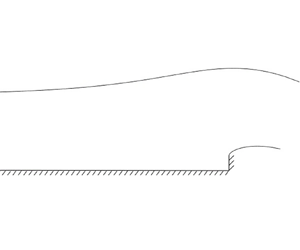
7. Extension to weir flows
For weir flows, as depicted in figure 8(a), we can employ the revision to the complex velocity  $\zeta$ that incorporates the improved form for the behaviour of the jet far downstream. The variables are non-dimensionalised, resulting in unit depth and velocity far upstream as earlier, in the waterfall case. We retain (2.3) to relate $f$ and $t$; and their complex planes (cf. figures 8b,c) are very similar to those used for the waterfall.

Figure 8. Complex planes for weir flows: (a)  $z$-plane, (b) $f$-plane, (c) $t$-plane.
Dias & Tuck (Reference Dias and Tuck1991) present supercritical solutions for this weir problem, utilising the same expansion for the assumed behaviour of the jet far downstream as in their waterfall calculations (i.e.  $\zeta \sim f^{1/3}$ as $\phi \rightarrow +\infty$). As seen earlier, for the jet we take
 \begin{equation} \zeta \sim \mathrm{i}(3G)^{1/3} f^{1/3} + u_{\infty} + C f^{{-}1/3} \quad \mathrm{as} \ \phi \rightarrow +\infty, \end{equation}
where  $u_{\infty }$ and $C$ are unknown constants. It is important to note that the constant term $u_{\infty }$ in this expression is unknown here (in contrast to the waterfall case, where it is known to be $1+{G}/{2}$). This is due to the unknown contribution (or rather, reduction) to the horizontal momentum flux provided by the vertical weir wall. It can be checked that the following form for $\zeta$ satisfies the necessary conditions for the supercritical weir flow far upstream, downstream and inside the corner at the origin:
 \begin{equation} \zeta={-}\mathrm{i} \left(\frac{t-t_O}{1-tt_O}\right)^{1/2}(1+(1+t)^{2\lambda/{\rm \pi}}\,B(t)), \end{equation}
where
 \begin{equation} B(t)=\left(\frac{1}{\rm \pi}\right)^{1/3}(-\log(c(1+t^{2})))^{1/3}l_1(t) + l_2(t) + \sum_{n=0}^{\infty}{a_n t^{n}}(-\log(c(1+t^{2})))^{{-}1/3}, \end{equation}
and  $l_1$ and $l_2$ are the linear functions
 \begin{equation} l_1(t)=\operatorname{Re}(m_1)+t\operatorname{Im}(m_1),\quad l_2(t)=\operatorname{Re}(m_2)+t\operatorname{Im}(m_2), \end{equation}
with
 \begin{align} m_1={-}(3G)^{1/3}2^{-\lambda/{\rm \pi}}\mathrm{e}^{-\mathrm{i} \lambda/2}\left(\frac{1-\mathrm{i} t_O}{\mathrm{i} - t_O}\right)^{1/2},\quad m_2=2^{-\lambda/{\rm \pi}}\mathrm{e}^{-\mathrm{i} \lambda/2}\left(\mathrm{i} u_{\infty}\left(\frac{1-\mathrm{i} t_O}{\mathrm{i} - t_O}\right)^{1/2}-1\right). \end{align}
Here,  $t_O$ denotes the point in the $t$-plane corresponding to the origin in the $z$-plane. In (7.3) and (7.5a,b), the constants $u_{\infty }$ and $a_n$, $n=0,1,2,\ldots$ are to be found. The solution (7.2)–(7.5a,b) is formed similarly to the solution for the waterfall of § 4. Here, the difference for the weir is the need to satisfy the condition of flow inside the corner at the origin of the $z$-plane.
The constant  $u_{\infty }$ can be found by adding an extra equation to the system. This constraint is derived similarly to (3.6), taking care to include the pressure force due to the vertical portion of the wall in the horizontal momentum balance. Then the extra equation to be satisfied is
 \begin{equation} u_{\infty}= 1 + \left.\frac{G}{2} - \int_0^{w} \, p\right|_{\psi=0} \, \mathrm{d} s, \end{equation}
where  $s$ is the displacement from the origin along the vertical wall, and $w$ denotes the height of the vertical weir wall. The pressure $p$ along this wall can be found via
 \begin{equation} p = \tfrac{1}{2} (1- |\zeta|^{2}) + G(1-y). \end{equation}
 As before, we truncate the series in the complex velocity  $\zeta$ after $N$ terms. We impose the height, $w$, of the vertical weir wall and so leave $t_O$ as an unknown to be found as part of the solution. We also wish to find $u_{\infty }$ – overall we have $N+2$ unknowns to find. Satisfying the Bernoulli condition along the free surfaces at $N$ collocation points, along with imposing the height of the vertical weir and the condition (7.6) on $u_{\infty }$, results in $N+2$ equations in $N+2$ unknowns. The $A$-method (introduced in the previous section) can also be employed here to improve coefficient decay.
Application of the revised form for the complex velocity leads to free-surface profiles that are very similar to those obtained by Dias & Tuck (Reference Dias and Tuck1991) for supercritical weir flows. Figure 9 shows profiles obtained for a weir wall height of  $w=0.2$ with various values taken for $G$. Note here that for $G=0.64$ we have two supercritical solutions. This agrees with the findings of Dias & Tuck (Reference Dias and Tuck1991): for sufficiently large values of $w$ and Froude numbers sufficiently close to 1, we obtain two solutions – a waterfall-type solution (cf. figures 9a,b) and a solitary-wave-type solution (cf. figure 9c). The difference between these two solution types is characterised by the ‘bump’ in the free surface for the solitary-wave type. In particular, the latter solution type heads towards a limiting configuration where there is a stagnation point (with difficulty in obtaining such solutions due to the unknown location of the stagnation point), which is conjectured and discussed by Dias & Tuck (Reference Dias and Tuck1991). Figure 10 shows many solutions by focusing on the values obtained for $y^{\star }$ (the value of $y$ corresponding to the point $\psi =1$ and $\phi =0$) plotted against the Froude number, for different choices of the physical weir wall height $w$. This may be compared with figure 9 of Dias & Tuck (Reference Dias and Tuck1991), which shows similar curves but instead for different choices of $t_{O}$, marking the position of the corner of the weir in the $t$-plane. As $t_{O}$ increases towards 1, the weir height decreases to zero. A qualitative comparison of the curves shows similar features.

Figure 9. Free-surface profiles for  $w=0.2$, $N=200$, $c=0.2$. (a) $G = 0.25$, $y^{\star }=1.25$. (b) $G=0.64$ (or $F=1.25$), $y^{\star }=1.32$. (c) $G=0.64$ (or $F=1.25$), $y^{\star }=1.47$.

Figure 10. Plots of  $y^{\star }$ (the value of $y$ at the point corresponding to $\psi =1$ and $\phi =0$) against $F$ for $N=99$ (the $A$-method has been applied) and $c=0.2$. Here, we plot trends with the Froude number $F$ for comparison with figure 9 of Dias & Tuck (Reference Dias and Tuck1991).
From figure 10, it can also be observed that for sufficiently tall weir walls (e.g.  $w=0.2$), there is a maximum value for $G$ above which (or a minimum value for $F$ below which) a solution cannot be obtained. These maximum values of $G$ correspond to maximum values of the unknown constant $u_{\infty }$ for the same wall height (cf. figure 11). It is interesting to note that for a particular value of $G$ for which there exist two supercritical solutions (e.g. figures 9b,c), the values obtained for the unknown constant $u_{\infty }$ are very similar despite resulting in very different free-surface profiles: one of waterfall type and the other of solitary-wave type. This is due to the global nature of the constant $u_{\infty }$ for the flow.

Figure 11. Plots of  $u_{\infty }$ against $G$ with $N=99$ (the $A$-method has been applied) and $c=0.2$ for various wall heights. The dashed line is $1+G/2$ (the value of $u_{\infty }$ for the waterfall, i.e. when $w=0$).
More generally, figure 11 shows the increase in  $u_{\infty }$ as the wall height $w$ decreases, whilst $u_{\infty }$ always remains less than $1+G/2$ (the value of $u_{\infty }$ for the waterfall), as expected. It should be noted that the value of $u_{\infty }$ appears to converge as $N$ increases – cf. table 1 for the case where $G=0.25$, $w=0.2$ and $c=0.2$. For each wall height, the value of $u_{\infty }$ also increases as $G$ increases, until a maximum value of $u_{\infty }$ (as mentioned above) is reached. In the absence of gravity, an exact solution can be found (cf. equations (17) and (18) of Dias & Tuck Reference Dias and Tuck1991) and then we can integrate the pressure $p=\frac {1}{2}(1-|\zeta |^{2})$ along the vertical weir wall in order to obtain $u_{\infty }$, the (finite) value of the horizontal velocity far downstream. Whilst the constant $u_{\infty }$ is not involved in the complex velocity form in the case of zero gravity, this physical quantity is still relevant and allows us to compare the results obtained through the exact and numerical solutions as $G\rightarrow 0$. The lines on figure 11(a) have been extrapolated to $G=0$ to facilitate this comparison, and table 2 gives the values of $u_{\infty }$ obtained through the exact solution – the values agree to order $10^{-3}$.
Table 1. Values obtained for  $u_{\infty }$ for various values of $N$ where $G=0.25$, $w=0.2$ and $c=0.2$.

Table 2. Comparison of values obtained for  $u_{\infty }$ when $G=0$ via the exact solution and numerical solution.

The effect of the revised form for the complex velocity  $\zeta$ can be seen in the free-surface profiles of figure 12. This figure compares the profiles obtained through the Dias & Tuck (Reference Dias and Tuck1991) form for $\zeta$ with the profiles obtained through use of the revised $\zeta$ form (along with use of the $A$-method). Also, note that both are extrapolated free-surface profiles, and the revised form leads to a jet that appears to approach a more parabolic shape. As in the case of the waterfall, whilst the revised complex velocity ansatz leads to very similar profiles when the number of mesh points used for plotting is the same as used in finding the unknown coefficients, the improvements observed when extrapolating the profiles downstream point towards great computational benefit from the revised $\zeta$ form.

Figure 12. Comparison of extrapolated weir free-surface profiles for  $G=0.25$, $c=0.2$ and $w=0.1$. The $A$-method has been utilised here for the revised $\zeta$ free surfaces only, i.e. $N=399$ for the revised $\zeta$ case, and $N=400$ for the Dias & Tuck (Reference Dias and Tuck1991) free surfaces. The two circles are the last two points of the non-extrapolated profiles.
8. Conclusions
Overall, the forms for the complex velocity that are adopted by Dias & Tuck (Reference Dias and Tuck1991) for the waterfall and supercritical weir have been improved to better encapsulate the behaviour of the free-falling jet. Visually, this is evident in figures 4 and 12, where the new extrapolated free-surface profiles are compared with those of Dias & Tuck (Reference Dias and Tuck1991) and (in the case of the waterfall) the asymptotic solution of Clarke (Reference Clarke1965). Employing the revised complex velocity forms also has great computational benefits since the resulting free surface profiles can be extrapolated, so we can reach further downstream without necessarily having to use a huge number of collocation points and solve for a huge number of unknown coefficients. Moreover, it has been demonstrated that the effectiveness of the overall numerical method is greatly improved by obtaining carefully the  $y$-values at the collocation points and by utilising the $A$-method (the addition of the unknown constant $A$ in the complex velocity, cf. (6.2)), thereby improving the coefficient decay of the truncated series.
Funding
B.S. acknowledges financial support from the Austrian Research Promotion Agency (project COMET-K2 InTribology, FFG-No. 872176, project coordinator: AC2T research GmbH, Wiener Neustadt, Austria).
Declaration of interests
The authors report no conflict of interest.


 Open access