2.1. Flow solver: large-eddy simulation (LES)

The dimensionless LES equations are obtained by filtering of the 3-D incompressible Navier–Stokes equations. The continuity and the Navier–Stokes equations are as follows:

(2.1)\begin{gather}\frac{{\partial {{\bar{u}}_i}}}{{\partial {x_i}}} = 0,\end{gather}

(2.2)\begin{gather}\frac{{\partial {{\bar{u}}_i}}}{{\partial t}} + \frac{\partial }{{\partial {x_j}}}({\bar{u}_i}{\bar{u}_j}) ={-} \frac{{\partial \bar{p}}}{{\partial {x_i}}} + \upsilon \frac{{{\partial ^2}{{\bar{u}}_i}}}{{\partial {x_j}\partial {x_j}}} - \frac{{\partial {{\bar{\tau }}_{ij}}}}{{\partial {x_j}}},\end{gather}

where u_i and u_j are the ith and jth components of the instantaneous dimensionless velocity vector (i, j = 1, 2, 3), respectively, x_i is the spatial location vector in the ith direction, p is the dimensionless pressure, υ is the coefficient of kinematic viscosity of the fluid, which is the inverse of the Reynolds number in the program, and the overbar represents time averaging. The subgrid-scale (SGS) stress ${\bar{\tau }_{ij}}$ results from filtering of the nonlinear convective fluxes. This term reflects the influence of the SGS turbulence on the large-scale turbulence structures. The SGS stress ${\bar{\tau }_{ij}}$ is calculated from the eddy viscosity relationship as

(2.3)\begin{equation}{\tau _{ij}} = {\bar{u}_i}{\bar{u}_j} - \overline {{u_i}{u_j}} ={-} {\upsilon _{SGS}}\left( {\frac{{\partial {{\bar{u}}_i}}}{{\partial {x_j}}} + \frac{{\partial {{\bar{u}}_j}}}{{\partial {x_i}}}} \right) + \frac{1}{3}{\delta _{ij}}{\bar{\tau }_{kk}},\end{equation}

where δ_ij = 1 when i = j, and υ_SGS is the SGS viscosity, being computed from the dynamic SGS model proposed by Germano et al. (Reference Germano, Piomelli, Moin and Cabot1991).

In this study, the second version of a code called the ‘large eddy simulation on curvilinear coordinates’ (LESOCC2), which was first developed at the Institute for Hydromechanics, Karlsruhe Institute of Technology, Germany (Breuer & Rodi Reference Breuer, Rodi, Voke, Kleiser and Chollet1994; Fröhlich & Rodi Reference Fröhlich, Rodi, Launder and Sandham2002), is used for the simulations. In this code, the governing equations were discretised by the finite-volume method on non-staggered curvilinear grids. The details of the discretisation of the LESOCC2 are available elsewhere (Fang et al. Reference Fang, Bai, He and Zhao2014, Reference Fang, Han, He and Dey2018).

2.2. Vegetation movement solver: immersed boundary method (IBM)

The ‘direct-forcing immersed boundary method’ is used to describe the fluid–solid interaction between the flow and the plants (Peskin Reference Peskin1972; Mohd-Yusof Reference Mohd-Yusof1997; Fadlun et al. Reference Fadlun, Verzicco, Orlandi and Mohd-Yusof2000). Each plant is modelled as a series of pellets composed of the IBM boundary grids (figure 1).

Figure 1. A section of the pellet that creates a single plant. Boundary grids are the grids filled with hatch marks.

The momentum equation of the boundary grids can be written as follows:

(2.4)\begin{equation}\frac{{\partial \boldsymbol{u}}}{{\partial t}} + (\boldsymbol{u} \boldsymbol{\cdot}{\nabla})\boldsymbol{u} ={-} {\nabla}p + (\upsilon + {\upsilon _{\textrm{SGS}}}){\nabla ^2}\boldsymbol{u} + \boldsymbol{f},\end{equation}

where u is the velocity vector of boundary grids, ${\nabla}^{2}$ is the Laplace operator and f is the forcing source term. The terms in bold represent vectors. Equation (2.4) can be discretised in time using the direct-forcing method as follows:

(2.5)\begin{equation}\frac{{{\boldsymbol{u}^{n + 1}} - {\boldsymbol{u}^n}}}{{\Delta t}} = \textrm{RH}{\textrm{S}^{n + {1 / 2}}} + {\boldsymbol{f}^{n + {1 / 2}}},\end{equation}

where RHS is the sum of the convective and viscous terms and the pressure gradient in (2.4), and uⁿ is the calculated velocity of the boundary grids at the nth time step. According to the force imposed on the boundary grids at the nth time step, their state of motion can be analysed and the velocity of the grids at the (n + 1)th time step v^{n +1} can be deduced (see § 2.3). According to (2.5), letting u^{n +1} = v^{n +1}, the body force f can be calculated as

(2.6)\begin{equation}{\boldsymbol{f}^{n + {1 / 2}}} ={-} \textrm{RH}{\textrm{S}^{n + {1 / 2}}}\textrm{ + }\frac{{{\boldsymbol{v}^{n + 1}} - {\boldsymbol{u}^n}}}{{\Delta t}}.\end{equation}

2.3. Movement and force analysis of plants

In the numerical model, a single plant is composed of solid sphere pellets connected with disembodied ropes (figure 2a). Each pellet is created by multiple IBM boundary grids. This structure can be used to simulate a submerged plant with a thin, soft stem and clumped leaves, such as Ceratophyllum demersum (figure 2b).

Figure 2. (a) Shape of the plants in the numerical model. The fine lines in the figure do not exist in the numerical model, but are realised by constraining the relative motion between the pellets. (b) C. demersum. By varying the number and diameter of the pellets contained in a single plant in (a), different shape characteristics of the plants can be simulated.

The pellets obstruct the flow, changing its momentum and receiving the reaction force of the flow. In addition, they are also subject to buoyancy, gravity and pulling force used to restrain the relative movement of the adjacent pellets. The rotation of an individual pellet is severely limited by the existence of the rope tensions. To be explicit, when the straight line of the tension does not pass through the centre of the pellet due to rotation, the torque generated by the tension dominates all the torques applied to the pellet. It causes the pellet to rotate again to the state where the tensions pass through the centre of the pellet. Therefore, a pellet cannot rotate to a large angle or at a high angular velocity. This is consistent with the actual observation in the physical model study described in § 3. Based on this, the influence of the torque is ignored in the force analysis of the pellet. By analysing the momentum of a single pellet, the following equation can be obtained:

(2.7)\begin{equation}\frac{{\textrm{d}{\boldsymbol{V}_l}}}{{\textrm{d}t}} = {\boldsymbol{F}_l} + {\boldsymbol{T}_l} - {\boldsymbol{T}_{l - 1}},\end{equation}

where V_l is the velocity vector of the lth pellet (from the top to the bottom), F_l is the vector sum of the force of flow on the lth pellet (that is, the force calculated in § 2.2), the buoyancy and the gravity of the pellet, and T_l is the tension of the lth rope (from the top to the bottom), taking the direction of the pulling force of the rope on the lth pellet as the positive direction. The force analysis of the lth pellet is shown in figure 3.

Figure 3. Dynamics of the lth pellet and its adjacent pellets. The blue arrows represent the force vectors, the red arrows represent the unit vectors in the direction of the ropes, and the green arrows represent the velocity vectors. The physical parameters represented by the notation in the figure are explained in § 2.3.

Since (2.7) is not closed, the dynamic state of a single pellet cannot be accurately solved, and the motion constraint equations of the adjacent pellets need to be added. According to the motion constraints of the adjacent pellets, the following equations can be obtained:

(2.8)\begin{gather}{\boldsymbol{V}_l}\boldsymbol{\cdot }{\boldsymbol{e}_{l - 1}} = {\boldsymbol{V}_{l - 1}}\boldsymbol{\cdot }{\boldsymbol{e}_{l - 1}},\end{gather}

(2.9)\begin{gather}\frac{{\textrm{d}{\boldsymbol{V}_l}}}{{\textrm{d}t}}\boldsymbol{\cdot }{\boldsymbol{e}_{l - 1}} = \frac{{\textrm{d}{\boldsymbol{V}_{l - 1}}}}{{\textrm{d}t}}\boldsymbol{\cdot }{\boldsymbol{e}_{l - 1}},\end{gather}

(2.10)\begin{gather}|{{\boldsymbol{T}_{l - 1}}} |= \frac{{{{(|{{\bf (}{\boldsymbol{V}_{l - 1}} - {\boldsymbol{V}_l}) \times {\boldsymbol{e}_{l - 1}}} |)}^2}}}{{{R_{l - 1}}}},\end{gather}

where e_{l −1} is the unit vector in the direction of the (l − 1)th rope, and R_{l −1} is the length of the (l − 1)th rope. According to (2.7)–(2.10), the forces and instantaneous acceleration of the pellet, a_l = dV_l/dt, can be obtained. Assuming that the force on the pellet remains constant within a time step, the equations of motion of the pellet can be discretised in time as follows:

(2.11)\begin{gather}\boldsymbol{V}_l^{n + 1} = \boldsymbol{V}_l^n + \Delta t\,\boldsymbol{a}_l^n,\end{gather}

(2.12)\begin{gather}\boldsymbol{x}_l^{n + 1} - \boldsymbol{x}_l^n = \Delta t\,\boldsymbol{V}_l^n + \frac{{\Delta {t^2}\,\boldsymbol{a}_l^n}}{2},\end{gather}

where $\boldsymbol{x}_l^n$ is the displacement of the lth pellet at the nth time step. According to (2.12), the position of the pellets at each time point can be obtained.

Because the model developed in this study cannot simulate the collision between clumped leaves, it is only suitable for plants with a single stem, and not for plants with bifurcate stems. Therefore, the present model can be improved as a future scope of this study involving the collision of leaves. Nevertheless, the model still has a wide adaptability, because the number and diameter of clumped leaves for each plant can be set to different values.

3.1. Physical model study

In order to verify the accuracy of the numerical model, a physical model study was designed to simulate flow with vegetation. The experimental results were compared with the numerical model results. The experiment was carried out in a long rectangular tilting flume with a length of 16 m and a width of 0.5 m having a bed slope of 0.0025. A flow stabiliser and circulation device were provided upstream and downstream of the flume, respectively. Previous studies have shown that the influence of submerged vegetation on the flow velocity is affected by the relative submergence of plants, that is, the ratio of flow depth H to vegetation height h (Nepf & Vivoni Reference Nepf and Vivoni2000). In natural rivers, most of the submerged plants are found in the range of shallow submergence (1 < H/h < 5) (Chambers & Kalff Reference Chambers and Kalff1985; Duarte Reference Duarte1991). In order to simulate the actual situation in the experiment, we set the flow depth and the vegetation height as 0.2 and 0.1 m, respectively, creating a relative submergence H/h = 2. Each plant was made of five smooth solid polypropylene pellet spheres (mass density ρ = 0.97 × 10³ kg m⁻³ and diameter D_s = 10 mm) in series. Each pair of pellets were connected by a polyester thread having a diameter of 0.3 mm and a length of 10 mm. The simulated vegetation was located in the middle of the flume. There were five rows of plants in the streamwise direction and nine rows in the spanwise direction. A total of 45 plants were set up in the experiment, consisting of 225 pellets. The spacing between the individual plants was set to half the plant height as 5 cm, as was done in previous studies (Favier et al. Reference Favier, Li, Kamps, Revell, O'Connor and Brücker2017). In this study, the simulated aquatic plants represented by C. demersum could not survive in the fast flow due to their soft stems, because they generally exist in rivers and lakes with low flow velocities (Hilt et al. Reference Hilt2018). In the physical model study, the incoming flow discharge was set to 0.01 m³ s⁻¹ (average velocity $\bar{u} = 0.1\;\textrm{m}\;{\textrm{s}^{ - 1}}$ and Reynolds number $Re = \bar{u}H/\upsilon = 20\,000$, where υ is the coefficient of kinematic viscosity of water).

In the experiment, the swaying and displacement of the plants were captured by a Canon EOS 50D camera with an imaging frequency of 30 Hz and were measured by an image processing program from the swaying angle of each plant in the captured images. The flow was measured by an acoustic Doppler velocimeter (ADV) at four vertical distances, 0.025, 0.075, 0.125 and 0.175 m. The sampling frequency of the ADV was set as 100 Hz for the data collection, and the acoustic frequency was 10 MHz. The velocities at these locations corresponded to the flow velocities near the bed, inside and outside of the vegetation canopy, and near the free surface. In the streamwise direction, the flow velocities at six locations were measured to analyse the velocity changes before, during and after the passage of flow through the vegetation. In the spanwise direction, in order to prevent the ADV probe from colliding with the plants, the measuring points were located at the middle of each two rows of the plants. The set-up of the physical model study is shown in figure 4.

Figure 4. Top view of the flume of the physical model study showing the zone of simulated vegetation within the dashed box. Circles in the dashed box represent the individual plants.

3.2. Numerical simulation

Numerical simulations were carried out to simulate the flow–vegetation interaction in the vegetation-covered zone of the flume (figure 4). In order to avoid disturbances near the inlet boundary and so that the simulation of the flow–vegetation interaction remained unaffected, a flow buffer zone 0.2 m long was kept upstream of the vegetation zone. In addition, to study the flow characteristics after passing through the vegetation zone, a space of length 0.2 m was allowed downstream of the vegetation. The overall size of the calculation domain was 0.6 m (x) × 0.5 m (y) × 0.2 m (z). The calculation domain and the simulated vegetation in the numerical simulation are shown in figures 5(a) and 5(b). Previous studies showed that the grid scale of the LES model should be between the Kolmogorov scale η (also called the dissipative scale, l_d) and the energy-containing scale l_e (Kolmogorov Reference Kolmogorov1941; Zhang et al. Reference Zhang, Cui, Xu and Xu2005). These scales can be obtained from the dimensional analysis as

(3.1)\begin{gather}{l_d} = \eta \sim {\left( {\frac{{{\upsilon^3}}}{\varepsilon }} \right)^{1/4}},\end{gather}

(3.2)\begin{gather}{l_e} \sim \frac{{{{u^{\prime}}^3}}}{\varepsilon },\end{gather}

where u′ is the root mean square of the velocity fluctuations and ε is the TKE dissipation rate, which can also be obtained using the dimensional analysis as

(3.3)\begin{equation}\varepsilon \sim \frac{{{u^4}}}{\upsilon },\end{equation}

where u is the time-averaged flow velocity. Using (3.1)–(3.3), it can be estimated that the side length of the grids should be between 10⁻³ and 10⁻⁵ m. Complying with this requirement, considering the computational efficiency and in view of the fact that the pellets constituting the plant should not contain too few IBM boundary grids, the side length of the grid was set to be 1 mm in this study.

Figure 5. (a) Computational set-up of flow with vegetation and (b) the xz plane of two single plants with grids used in the simulation.

The boundary conditions of the momentum equation were as follows. In the x direction, the Dirichlet boundary was used upstream, implying the flow takes place from the boundary grids in the calculation domain with a constant bulk channel velocity U_b = Q/WH = 0.1 m s⁻¹, where Q is the flow discharge, W is the channel width and H is the flow depth. In addition, in order to study the relationship between the flow velocity and the plant movement, five additional numerical simulations were carried out with the bulk flow velocity U_b = 0.05, 0.06, 0.07, 0.08 and 0.09 m s⁻¹. The corresponding Reynolds numbers ranged over 10 000–18 000. The wall function was adapted at the bottom and the spanwise direction (y direction) in order to match with the physical model study, and the Manning roughness coefficient of the channel was the same as that in the physical model study (set as n = 0.045 s m^−1/3). The free surface was assumed to be a rigid lid with a slip condition, which is usually used to simulate the free surface of flow with minute fluctuation.

According to the experimental set-up, the methods of the physical model study and the numerical simulation, and considering the tolerance of flexible vegetation to flow velocity, nine groups of experiments are conducted in this study, as shown in table 1. Among them, the RVMRE20(V) case is a rigid vegetation model of the numerical simulation in which the vegetation remains stationary in the initial vertical state under the flow condition of Re = 20 000, while the RVMRE20(I) case is another rigid vegetation model of the numerical simulation under the flow condition of Re = 20 000 in which the vegetation remains stationary in an inclined state. The RVMRE20(I) case is set up to compare with the FVMRE20 case to distinguish the effects of the vegetation tilt and swaying on the flow conditions. To ensure that the effect of vegetation tilt on flow is consistent in the two cases, the inclination angles of the plants in the RVMRE20(I) case are set according to the time-averaged values of their swaying angles, ${\bar{\theta }_x}$, simulated by the FVMRE20 case (calculated in § 4.2).

Table 1. List of the experiments conducted in this study.

In the following sections, the accuracy of the numerical model is verified and the flow–vegetation interaction is analysed in detail according to the results of the nine groups of experiments. Specific verification and analysis are carried out as follows. The results of the PMRE20 and FVMRE20 cases are compared to verify the simulation effects of the numerical model on the flow–vegetation interaction (§ 4). In terms of the effects of the flow on the vegetation movement, six groups of numerical simulations of the flexible vegetation model (FVMRE20–FVMRE10 cases) with different flow velocities are analysed (§ 5.1). In terms of the impact of the vegetation motion on the flow, the simulation results of the rigid vegetation model of the numerical simulations (RVMRE20(V) and RVMRE20(I) cases) and the flexible vegetation model of the numerical simulation (FVMRE20 case) are compared. The influence of vegetation deformability on the flow velocity field, turbulence structure and energy transmission is examined (§ 5.2). According to these, the difference of flow resistance between the flexible and the rigid vegetation cases can be further obtained. Based on the analysis of the above results, the law governing the variation of vegetation canopy height caused by variabilities of the flow conditions and the influence of the vegetation deformability on the drag force acting on the vegetation due to the flow are summarised (§ 5.3).

In order to facilitate the model validation and the analysis of the results in the following sections, 45 plants are sorted in ascending order according to the spanwise distance (that is, y coordinate) as the main condition, and the streamwise distance (that is, x coordinate) as the secondary condition. The simulated vegetation zone in the physical model study, the calculation domain of the numerical simulations (RVMRE20(V), RVMRE20(I) and FVMRE20–FVMRE10 cases) and their dimensionless coordinates are shown in figure 6(a–c).

Figure 6. (a) Elevation view of the simulated vegetation zone (dashed box in figure 4) in the physical model study. The hollow circles represent the pellets that simulate the plants and the squares with crosses at the centre represent the ADV measuring points. The x and z are the streamwise and vertical distances, respectively, taking the dimensionless coordinate as z/D_s with the initial position of the vegetation canopy as 0 (that is, the vertical distance of 10D_s from the bed). (b) Top view of the simulated vegetation zone in the physical model study. All markings are the same as in (a). The y is the spanwise direction, taking the dimensionless coordinate as y/D_s with the initial position of the middle row of plants along the width of the flume (plants numbers 21–25) as 0. (c) Elevation view of the numerical simulation calculation domain. In the numerical simulation and the physical model study, the coordinate axes and directions are the same, and their values correspond to each other.

4.1. Flow velocity

Figure 7 shows the time-averaged streamwise velocity ${\bar{u}_x}$ of flow at different locations measured in the PMRE20 case and the computed values of ${\bar{u}_x}/{U_b}$ at the corresponding positions in the FVMRE20 case. The results show that, compared with the physical model study, the prediction error of this numerical model is less than 5%. According to the results of the FVMRE20 case, the numerical model has a good simulation effect on the flow velocity in the low-velocity zone below the vegetation canopy height and in the high-velocity zone above the vegetation canopy height.

Figure 7. Comparison of the dimensionless time-averaged streamwise velocity ${\bar{u}_x}/{U_b}$ of flow at all 192 ADV measuring points in the PMRE20 case and the computed value of ${\bar{u}_x}/{U_b}$ at the corresponding positions in the FVMRE20 case. The solid line is the y = x auxiliary line, representing the zero error. The two dotted lines are y = 1.05x and y = 0.95x auxiliary lines, representing 5% error.

In order to verify whether the numerical model can effectively calculate the difference of the flow velocity between the inside and outside of the vegetation canopy, figure 8 compares the time-averaged streamwise velocity ${\bar{u}_x}$ of flow obtained from the PMRE20 and FVMRE20 cases at 24 measuring points on the y/D_s = 2.5 plane for different x/D_s values. As compared with the PMRE20 case, the prediction errors of the FVMRE20 case of ${\bar{u}_x}/{U_b}$ above the vegetation canopy height are 0.76%, 0.34%, 0.29%, 5.38%, 1.12% and 4.63%, respectively. The prediction errors of the flow velocity below the canopy height are 3.73%, 9.51%, 9.49%, 3.66%, 10.65% and −6.55%, respectively. The calculation error of the FVMRE20 case for the difference between ${\bar{u}_x}$ inside and outside of the vegetation canopy is less than 0.1U_b, that is, the maximum error is less than 10% of the bulk channel velocity.

Figure 8. (a–f) Vertical distributions of the dimensionless time-averaged streamwise velocity ${\bar{u}_x}/{U_b}$ on the y/D_s = 2.5 plane for different x/D_s. The triangle symbols represent the measured results of the physical model study. The solid lines represent the simulation results of the FVMRE20 case.

The velocity distribution characteristics of vegetated flow have been studied extensively. Among them, the most representative one is Ghisalberti & Nepf (Reference Ghisalberti and Nepf2002), who gave the velocity distribution in the mixing layer near the vegetation canopy height under different flow conditions. Their study showed that the dimensionless flow velocity $\hat{U} = (U - \bar{U})/\Delta U$ presents a uniform hyperbolic tangent distribution in the mixing layer (figure 9), where U is the time-averaged flow velocity, $\bar{U} = ({U_1} + {U_2})/2$, with U ₁ and U ₂ being the low and high stream velocities in the mixing layer, respectively. Since the mixing layer thickness is different under different flow conditions, the vertical coordinate should also be made dimensionless to facilitate comparison, namely, $\hat{z} = (z - \bar{z})/\theta$, where z is the initial vertical coordinate, and $\bar{z}$ is the vertical coordinate, where $U = \bar{U}$, and θ is defined as

(4.1)\begin{equation}\theta = \int_{ - \infty }^\infty {\left[ {\frac{1}{4} - {{\left( {\frac{{U - \bar{U}}}{{\Delta U}}} \right)}^2}} \right]\textrm{d}z} .\end{equation}

Figure 9. Time-averaged flow velocity distributions for the FVMRE20–FVMRE10 cases. The comparison between the simulated velocity profiles and the hyperbolic tangent flow velocity curve (Ghisalberti & Nepf Reference Ghisalberti and Nepf2002) is satisfactory.

Comparing the dimensionless flow velocity distribution of the FVMRE20–FVMRE10 cases in the mixing layer with the hyperbolic tangent flow velocity curve obtained by Ghisalberti & Nepf (Reference Ghisalberti and Nepf2002), the simulation effect of this study on the flow velocity distribution with vegetation under different flow conditions can be verified (figure 9).

In figure 9 under various flow conditions (FVMRE20–FVMRE10 cases), the velocity distribution in the mixing layer is consistent with the hyperbolic tangent velocity curve in Ghisalberti & Nepf (Reference Ghisalberti and Nepf2002). It can be seen that the velocity distribution simulated by the model in this study corresponds with the prediction results of the velocity distribution of vegetation flow in previous studies.

4.2. Vegetation movement

Since the upstream flow boundary has a constant discharge in the numerical simulation, the movement of vegetation is not due to the change of discharge, but due to the velocity fluctuation. The velocity fluctuation is highly random. The fluctuations that result from any two physical experiments and simulation cases cannot be exactly the same. Therefore, the physical model study and the numerical simulation are not able to get exactly the same simulation results of vegetation movement. Hence, we only compare the movement features of vegetation simulated in the FVMRE20 case with those obtained from the physical model study in a period of time from the perspective of statistics (figure 10a,b).

Figure 10. (a) Plant movement at a certain moment simulated in the FVMRE20 case. In order to avoid visual confusion caused by the overlapping projections of multiple rows of plants, only the plants on the y = 0 plane are shown. (b) Plant movement at a certain moment obtained from the PMRE20 case. The coordinates of the plants are shown in figure 4(b).

Figure 11(a,c,e,g,i) shows the dimensionless streamwise offset Δx/D_s of the top of plants numbers 21–25 simulated in the FVMRE20 case and obtained from the physical model study. It can be observed that the average values of Δx/D_s simulated in the FVMRE20 case are consistent with those obtained from the physical model study within an error of range 10%. Since the average values of Δx/D_s can approximately represent the positions of the equilibrium force of the pellets in the average flow velocity field, the numerical model can be accurate and effective in simulating the force on the pellets. Comparing the variation range of Δx/D_s simulated in the FVMRE20 case with that obtained from the physical model study, it can be found that the variation range of Δx/D_s of the five plants simulated in the FVMRE20 case is generally larger than that obtained from the physical model study. This is accredited to the measurement frequency of the plant movement trajectory in the FVMRE20 case (f_{FVMRE 20} = 1000 Hz), which is much higher than that in the physical model study (f_PM = 1 Hz). This makes it more likely to capture the extreme values of Δx/D_s in the FVMRE20 case.

Figure 11. (a,c,e,g,i) Fluctuations of the dimensionless streamwise offset Δx/D_s of the top of plants numbers 21–25 over a period of dimensionless time 0 < t/(D_s/U_b) < 400 simulated in the FVMRE20 case and obtained from the physical model study. The blue dotted lines and red triangles represent the simulation results of Δx/D_s in the FVMRE20 case and the data plots of the physical model study, respectively. The blue and red solid lines are the mean values of Δx/D_s simulated in the FVMRE20 case and obtained from the physical model study, respectively. (b,d,f,h,j) Probability density distributions PD of the fluctuations of Δx/D_s of the top of plants numbers 21–25 simulated in the FVMRE20 case and obtained from the physical model study. The solid and dashed lines represent the PD curves of the fluctuations of Δx/D_s simulated in the FVMRE20 case and obtained from the physical model study, respectively.

Besides, figure 11(b,d,f,h,j) presents the probability density (PD) distributions of the fluctuations of Δx/D_s of the top of plants numbers 21–25 simulated in the FVMRE20 case and obtained from the PMRE20 case. As can be seen, for the first four plants (numbers 21–24), Δx/D_s obtained from the PMRE20 case is slightly smaller than that obtained from the FVMRE20 case, while for plant number 25 the PD curves obtained in the two cases are quite consistent. According to the PD curves, it can be calculated that, compared with the PMRE20 case, the errors of the mathematical expectation of Δx/D_s of plants numbers 21–25 in the FVMRE20 case are 4.86%, 8.33%, 5.29%, 5.34% and −2.37%, respectively. The errors of the median values are 4.60%, 8.55%, 6.77%, 6.96% and −1.02%, respectively.

Figure 12 compares of the distributions of the streamwise offset angle θ_x of plants numbers 21–25 relative to their initial positions simulated in the FVMRE20 case and obtained from the physical model study over a period of dimensionless time 0 < t/(D_s/U_b) < 400. It is evident that, in the θ_x distribution, the median and the mean values are almost the same in both the FVMRE20 simulation case and the physical model study. In addition, the distances between the median value and the upper and lower quartiles are almost the same, as are the distances between the maximum value and upper quartile, and between the minimum value and lower quartile. These indicate that, under the condition of constant unidirectional flow, the plants sway uniformly on both sides of the force balance point with a similar amplitude. The probabilities of swaying to both the sides (including upstream and downstream) are mostly the same. Comparing the simulation results of the FVMRE20 case with the results obtained from the physical model study, trends similar to those in figure 11 can be obtained. It indicates that, except for plant number 21, the mean values of θ_x of the other plants are quite similar in the two experiments (numerical and physical), with a maximum error of 9.24%, while the range of extreme values is slightly smaller in the physical model study, with a maximum error of 14.76%.

Figure 12. Comparisons of the distributions of the streamwise offset angles θ_x of plants numbers 21–25 simulated in the FVMRE20 case (the blue rectangular boxes) and obtained from the physical model (PM) (the orange rectangular boxes). The crosses in the boxes represent the median values θ_xm, the horizontal lines in the middle of the boxes represent the average value ${\bar{\theta }_x}$ and the small solid circles represent the statistically significant outliers. Since all the data were simulated in the FVMRE20 case and obtained from the physical model, the outliers are reliable values and have some significance in indicating the maximum swaying amplitude of the plants. The average value ${\bar{\theta }_x}$ in the box plot can represent the offset angle corresponding to the plant force balance position. The difference between the upper and lower edges of the straight line represents the maximum swaying amplitude Δθ_x of the plant.

According to the comparison of multiple indices, the results of the FVMRE20 simulation case and the physical model study are in good agreement. This numerical model can effectively simulate the movement of flexible plants under the flow–vegetation interaction.

5.1. Impact of flow conditions on vegetation movement

The flow velocity variation directly affects the forces acting on the plants – see § 2.3 and Luhar & Nepf (Reference Luhar and Nepf2011) – and also the state of the vegetation movement. With an increase in flow velocity, the turbulence intensity increases and vortex structure in the flow changes, which in turn affect the amplitude of the swaying of the plants. In order to study the difference of the states of the plant movement under different flow velocities, we compare the statistical distributional features of the streamwise and spanwise offset angles, θ_x and θ_y, of the plants simulated by the six types of numerical simulations (FVMRE20–FVMRE10 cases) in figures 13(a) and 13(b).

Figure 13. Movement of five plants (numbers 21–25) under different flow velocities. Distributions of (a) the streamwise swaying amplitude θ_x and (b) the spanwise swaying amplitude θ_y of the top of the plants. The six colours represent six cases with Reynolds numbers varying from 10 000 to 20 000, corresponding to the FVMRE10–FVMRE20 cases. The symbols used in the figure are same as in figure 12.

It is apparent from figures 13(a) and 13(b) that, as the flow velocity increases, the streamwise force balance angles θ_x of the five plants increase, that is, the plants need to tilt to a larger angle to balance the increased horizontal force (Wilson et al. Reference Wilson, Stoesser, Bates and Batemann Pinzen2003), while the spanwise force balance angles θ_y remain unchanged. Although the streamwise average force on the plants increases with the flow velocity (Luhar & Nepf Reference Luhar and Nepf2011), it has little effect on the spanwise average force. The maximum swaying amplitudes in the streamwise Δθ_x and the spanwise Δθ_y directions of the five plants increase clearly with an increase in flow velocity. This is attributed to the fact that, as the flow velocity increases, the turbulence in flow is intensified, and thus the maximum swaying amplitude of the plants enhances.

Under the same flow velocity condition, the streamwise force balance angles θ_x of the five plants decrease with an increase in their initial x coordinates, consistent with the results of the existing 2-D flexible vegetation models (Favier et al. Reference Favier, Li, Kamps, Revell, O'Connor and Brücker2017; O'Connor & Revell Reference O'Connor and Revell2019). However, the maximum swaying amplitudes in the streamwise Δθ_x and the spanwise Δθ_y directions of the downstream plants are not significantly different from those of the upstream plants. This indicates that, in the vegetation zone, the average force on the downstream plants is significantly weaker than that on upstream plants at various flow velocities. On the other hand, there is no significant difference in turbulence intensities between the upstream and the downstream vegetation zones in small vegetation patches.

Analysing the relation of the flow velocity $\bar{u}$, the position of the average force balance angle $\bar{\theta }$ of plants and the maximum swaying amplitude Δθ, the relation of the flow velocity, stress on the plants and turbulence intensity in the vegetation zone can be obtained. Luhar & Nepf (Reference Luhar and Nepf2011) obtained the analytical solution of the streamwise offset angle ${\bar{\theta }_x}$ by analysing the relationship between the stress and the deformation of flexible submerged vegetation.

According to the force balance analysis of the buoyancy, drag force and plant resistance to flow in Luhar & Nepf (Reference Luhar and Nepf2011), a simplified formula for calculating the vegetation streamwise offset angle ${\bar{\theta }_x}$ can be obtained:

(5.1)\begin{equation}\textrm{sin}\,{\bar{\theta }_x} = CU_b^2\ \textrm{co}{\textrm{s}^2}\,{\bar{\theta }_x},\end{equation}

where C is a value related to the plant's own properties (such as stem diameter, plant length, etc.) and the drag force coefficient C_D on flow (Blevins Reference Blevins1984). In this study, the value of C is related only to the location of plants. For the same plant, the value of C does not vary with Re. Therefore, the simulation results of the FVMRE10 case are used to determine the value of C for plants numbers 21–25, and the theoretical values of vegetation offset angles under other Re conditions are calculated from (5.1). The theoretical values are compared with the simulation results of FVMRE12–FVMRE20.

Figure 14(a) shows the variations of the streamwise offset angle ${\bar{\theta }_x}$ and the maximum swaying amplitude Δθ_x of plants numbers 21–25 with Reynolds number Re, and compares the results with the predicted results of ${\bar{\theta }_x}$ obtained by Luhar & Nepf (Reference Luhar and Nepf2011). It can be seen that, for plant number 21, the experimental results of this study match well with those predicted by Luhar & Nepf (Reference Luhar and Nepf2011) at various Reynolds numbers. However, for plants numbers 22–25, the matching is found to be good only when Re is small (Re < 18 000). When Re = 20 000, the streamwise offset angle ${\bar{\theta }_x}$ of this study is greater than that predicted by Luhar & Nepf (Reference Luhar and Nepf2011). This is attributed to the fact that, in Luhar & Nepf (Reference Luhar and Nepf2011), the drag force on the plant is directly related to the bulk flow velocity U_b in the channel. For plant number 21, the flow velocity at the plant location is fairly consistent with U_b. Therefore, the method of Luhar & Nepf (Reference Luhar and Nepf2011) can accurately predict the drag force on the plant and calculate the accurate value of ${\bar{\theta }_x}$ based on it. However, for downstream plants, due to the flow obstruction by the upstream plants, the flow velocity at the location of the plants reduces nonlinearly with Reynolds number. Therefore, it is erroneous to calculate the drag force on plants based on the bulk velocity U_b. In essence, the method of Luhar & Nepf (Reference Luhar and Nepf2011) is not suitable for the estimation of ${\bar{\theta }_x}$ of each plant in a plant cluster. Based on the results of the effects of plant clusters on the flow velocity reduction in this study (§ 5.2.1), the method of Luhar & Nepf (Reference Luhar and Nepf2011) can be improved to obtain an analytical solution of ${\bar{\theta }_x}$ for different plants in a plant cluster.

Figure 14. (a) Mean value of the streamwise offset angles ${\bar{\theta }_x}$ (force balance angle) of the five plants (numbers 21–25) as a function of Reynolds number Re and (b) maximum swaying amplitude Δθ_x of the five plants as a function of Reynolds number Re. Different symbols correspond to different plant numbers. The dotted lines in (a) are the predicted values of ${\bar{\theta }_x}$ obtained from the model of Luhar & Nepf (Reference Luhar and Nepf2011), and the dotted lines in (b) are the linear fitted lines.

Figure 14(b) shows the variations of the maximum swaying amplitude Δθ_x of plants numbers 21–25 with Reynolds number Re. It is evident that the maximum swaying amplitude Δθ_x of the plants increases linearly with Re. The gradients of the straight lines obtained by fitting linear curves are almost the same, indicating that the modes of the swaying amplitude Δθ_x of the upstream and downstream plants changing with Re are essentially the same. For a given Re, the values of the maximum Δθ_x of the five plants have no fixed relationship. The maximum Δθ_x difference between two adjacent plants is within 20°. This reveals that, at various Re, the turbulence intensity in the flow within the vegetation zone is roughly uniform and does not vary significantly in the downstream region in small vegetation patches (see § 5.2.2 for details).

5.2. Impact of vegetation movement on the flow structure

5.2.1. Averaged flow velocity field

The influence of the flexible vegetation movement on the flow velocity field can be divided into two parts. The first part is related to the change in flow velocity caused by the vegetation tilt under the action of flow impulse. It can be analysed by examining the simulation results obtained from the RVMRE20(V) and RVMRE20(I) cases. The other part is related to the disturbance of the flow caused by the swaying of vegetation around the average force balance position. It can also be analysed by inspecting the simulation results obtained from the RVMRE20(I) and FVMRE20 cases.

Figure 15(a–c) depicts the dimensionless streamwise time-averaged velocity structures ${\bar{u}_x}/{U_b}$ on the plane y/D_s = 0 (Y1) simulated numerically in the RVMRE20(V), RVMRE20(I) and FVMRE20 cases, respectively. Examining figure 15(a,b), it can be seen that the vegetation tilt eliminates the ribbon distribution of ${\bar{u}_x}$ within the vegetation zone and makes the velocity distribution within the vegetation more uniform. The canopy height of inclined vegetation decreases, but does not significantly change the ${\bar{u}_x}$ inside and outside the vegetation canopy. However, given that the effective volume occupied by the vegetation zone decreases, it can be predicted that the resistance of the vegetation to the flow decreases (specifically analysed in § 5.3). In essence, vegetation tilt does not significantly change the difference of ${\bar{u}_x}$ between the inside and the outside of the vegetation canopy, and therefore it does not significantly change the momentum and mass transport inside and outside of the vegetation canopy.

Figure 15. Dimensionless time-averaged streamwise velocity structures ${\bar{u}_x}/{U_b}$ on the Y1 plane simulated numerically in the (a) RVMRE20(V) (vertical rigid vegetation with Re = 20 000), (b) RVMRE20(I) (inclined rigid vegetation with Re = 20 000) and (c) FVMRE20 (flexible vegetation with Re = 20 000) cases. Owing to vegetation movement, the characteristic location Z2 (that is, the flow–vegetation interface) is not a fixed plane in (b and c).

Examining figure 15(b,c), it is evident that the swaying of vegetation further homogenises the distribution of ${\bar{u}_x}$ within the vegetation zone. At the same time, the average velocity ${\bar{u}_x}$ inside the vegetation decreases and ${\bar{u}_x}$ above the vegetation canopy increases, causing the difference between ${\bar{u}_x}$ inside and outside the vegetation canopy to enhance. Therefore, the swaying of the flexible vegetation around the force balance point is the main factor to intensify the energy and mass transport between the inside and outside of the vegetation canopy.

Figure 16 shows the vertical distributions of the double-averaged (spatially averaged in the spanwise direction) streamwise velocity ${\bar{u}_x}$ at various places in the vegetation zone, and upstream and downstream of the vegetation zone for different x/D_s. It is obvious that the flow velocity field is affected before the flow enters the vegetation zone, regardless of the vegetation being rigid or flexible. If the local banded distribution of velocity caused by plant shape is not considered, the velocity distributions obtained from the three simulation cases are similar at x/D_s = 17.5. The blocking effect of the vegetation on the flow can be reversed upstream, and it may be equivalent to the increase in the shear layer thickness near the bed surface.

Figure 16. (a–d) Vertical distributions of the dimensionless width-averaged streamwise velocity ${\bar{u}_x}/{U_b}$ within and downstream of the vegetation zone for different x/D_s. The solid lines represent the simulation results of the RVMRE20(I) case, the blue dotted lines represent the simulation results of the RVMRE20(V) case and the red broken lines represent the simulation results of the FVMRE20 case.

The flow velocity field inside the vegetation zone is more complex (figure 16b,c). It is noticeable that the velocity distributions computed from the RVMRE20(I) and FVMRE20 cases are consistent with those of Nepf (Reference Nepf2012) and Ghisalberti & Nepf (Reference Ghisalberti and Nepf2002). The effects of the vegetation on the flow can be equivalent to forming a mixing layer, in which the flow velocity ${\bar{u}_x}$ does not show a monotonic trend with the vertical distance. Unlike vertical rigid vegetation, the ${\bar{u}_x}$ with inclined rigid vegetation declines with an increase in the mixing layer thickness, but the ${\bar{u}_x}$ inside the mixing layer does not decrease significantly. Therefore, there is no significant change in velocity difference between the inside and the outside of the vegetation canopy. Besides, the vegetation tilt even tends to decrease the flow velocity above the canopy. It follows that the effect of vegetation tilt is to reduce the momentum loss of the flow compared to the vertical state (as predicted by Nepf (Reference Nepf1999)).

However, the swaying of flexible vegetation on the basis of tilt significantly increases the mixing layer thickness, the flow velocity above the canopy, and the velocity gradient inside and outside the vegetation canopy, and reduces the flow velocity within the vegetation. This means that the effect of swaying of vegetation is to intensify the KH instability near the canopy, and the mass and energy transfer inside and outside of the vegetation canopy. The oscillation of vegetation significantly increases the momentum consumption of the flow. It can be predicted that the swaying of vegetation increases the drag force on the flow, and thus the obstruction to flow is more obvious.

After the fluid has flowed out of the vegetation zone, the influence of the vegetation gradually weakens, and the effect of the vegetation on the flow can be equivalent to changing the boundary layer characteristics. In the three simulation cases, the results of the FVMRE20 case show that the swaying of vegetation has a more lasting effect on the flow. This indicates that the effect of swaying of vegetation is to significantly intensify its disturbance on the flow (see §§ 5.2.2 and 5.2.3 for details).

5.2.2. Turbulence structure

Vorticity is the curl of the flow velocity vector, which is an important hydrodynamic parameter to characterise the intensity and direction of the swirl in a flow (Wallace & Foss Reference Wallace and Foss1995). The vorticity can be calculated as follows:

(5.2) \begin{equation} \boldsymbol{\omega } = {\nabla} \times \boldsymbol{u } = \left( {\frac{{\partial {u_z}}}{{\partial y}} - \frac{{\partial {u_y}}}{{\partial z}}} \right)\boldsymbol{i} + \left( {\frac{{\partial {u_x}}}{{\partial z}} - \frac{{\partial {u_z}}}{{\partial x}}} \right)\boldsymbol{j} + \left( {\frac{{\partial {u_y}}}{{\partial x}} - \frac{{\partial {u_x}}}{{\partial y}}} \right)\boldsymbol{k},\end{equation}

where ω is the vorticity vector, u, u_x, u_y and u_z are the velocity vector and its components in the x, y and z directions, respectively, and i, j and k are the unit vectors in the x, y and z directions, respectively.

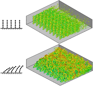
Figure 17(a–c) depicts the dimensionless vorticity structures ω_z/ω ₀ on the Z1 plane simulated in the RVMRE20(V) (z/D_s = −5), RVMRE20(I) (z/D_s = −7.5) and FVMRE20 (z/D_s = −7.5) cases, respectively, where ω_z is the vorticity component about the z axis and ω ₀ = U_b/D_s. From the simulation results of the RVMRE20(V) case (figure 17a), it is obvious that there are two rows of alternately generated vortices downstream of a single plant, forming a commonly known wake structure (Nikora Reference Nikora2010), in which the turbulence only occurs directly downstream of plant bodies. The two rows of vortices rotate in opposite directions and form a vortex street. Within the vegetation zone, the two rows of vortices move downstream with a minimal spreading in the spanwise direction. Between any two adjacent rows of the plants, ω_z vanishes. Downstream of the vegetation zone, ω_z decreases rapidly in a short distance. Besides, the two rows of vortices in opposite directions mix with each other and dissipate rapidly. Then, the flow pattern returns to the initial stable state within a short distance. The vorticity distribution of flow in vegetation obtained from the RVMRE20(I) case is consistent with the results obtained from the RVMRE20(V) case, that is, the vorticity is distributed in a ribbon and does not diffuse in the spanwise direction. Unlike the simulation results of the RVM cases, the vortices inside the vegetation simulated in the FVMRE20 case are larger, but more broken (figure 17c). The vortices are irregularly directed, and the magnitudes of ω_z of the two groups of adjacent vortices with opposite directions are different. The vegetation movement forms a jet structure, that is, not only is the turbulence distributed downstream of the plant bodies, but also the momentum is transmitted to the surrounding water body. In the spanwise direction, the magnitudes of ω_z are uniformly distributed; however, there is no ribbon distribution of the vorticity, as observed in figures 16(b) and 17(a), similar to that simulated in the RVM cases. This indicates that the vegetation movement causes vortex diffusion and mixing in the spanwise direction, even in the gap between the two adjacent rows of the plants.

Figure 17. Dimensionless vorticity structures ω_z/ω ₀ simulated in (a) the RVMRE20(V) case, (b) the RVMRE20(I) case and (c) the FVMRE20 case on the Z1 plane.

Since the vorticity distributions in the vegetation zone obtained from the RVMRE20(V) and RVMRE20(I) cases are similar, this implies that the plant tilt does not affect the vortex structure of flow in the vegetation zone. Therefore, the effects of the flexible vegetation on the vortex structure of flow are mainly realised by the swaying. Figure 18 compares the vortex structure of flow obtained from the RVMRE20(I) and FVMRE20 cases. Figure 18(a) shows that, when there is no swaying of vegetation, the vortex formed is mainly a small hairpin vortex (HP vortex). The vortex size is similar to the plant diameter. The KH instability at the fluid–vegetation interface is not strong enough to form large-scale KH vortices. According to figure 18(b), when the vegetation sways, the vortex scale significantly increases, and KH vortices with the same scale as the plant spacing are formed at the fluid–vegetation interface. These KH vortices are connected with the HP vortices and form the KH–HP vortex structures, in conformity with Tschisgale et al. (Reference Tschisgale, Löhrer, Meller and Fröhlich2021). Unlike Tschisgale et al. (Reference Tschisgale, Löhrer, Meller and Fröhlich2021), the spanwise swaying of the vegetation is considered in this study, making the computation of the spanwise transfer of the TKE more accurate (see § 5.2.4). The spanwise transfer of the TKE significantly increases the difference of velocity and pressure pulsations in different sections in the spanwise direction. Therefore, the spanwise scale of the KH vortices computed in this study is no larger than the plant spacing, being significantly smaller than those computed by Tschisgale et al. (Reference Tschisgale, Löhrer, Meller and Fröhlich2021).

Figure 18. Vortex structure of flow in the vegetation zone obtained from (a) the RVMRE20(I) and (b) the FVMRE20 cases. The vortex structure in the figure is represented by the iso surface of pressure fluctuation. The colour of the background flow field indicates the instantaneous velocity. The colour of the pressure pulsation iso surface indicates the velocity fluctuation.

The distribution of the HP vortex structure and the KH–HP vortex structure and their influence on the flow can be directly displayed by quantitatively comparing the eddy size at different positions under the condition of swaying and stationary vegetation. The eddy size in the inertial subrange is defined as the Taylor microscale λ_T, which is given by

(5.3)\begin{equation}{\lambda _T} = {\left( {\frac{{15\upsilon \overline {u^{\prime}u^{\prime}} }}{\varepsilon }} \right)^{0.5}},\end{equation}

where ε is the TKE dissipation rate (the same as in (3.1)), which can be estimated by using Kolmogorov's second hypothesis (Dey et al. Reference Dey, Das, Gaudio and Bose2012):

(5.4)\begin{equation}k_w^{5/3}E({k_w}) = C{\varepsilon ^{{2 / 3}}},\end{equation}

where k_w is the wave number, E(k_w) is the energy spectrum function that represents the TKE k′ to contain eddies of size l having wave number k_w (= 2π/l) and C is a constant, which is usually set as 0.5 (Monin & Yaglom Reference Monin and Yaglom2007). The energy spectrum function E(k_w) can also be regarded as the TKE k′ energy density of eddies with wave number k_w, which satisfies

(5.5)\begin{equation}k^{\prime} = \int_0^\infty {E({k_w})\ \textrm{d}{k_w}} .\end{equation}

Figure 19(a–d) compares the energy spectra E(k_w) of the FVMRE20 and the RVMRE20(I) cases at the height of the vegetation canopy directly above a row of plants (Y1) and in the middle of two rows of plants (Y2). It can be observed that Kolmogorov's −5/3 scaling law is satisfied in the inertial subrange of flow with vegetation for both the rigid and the flexible cases. It can therefore be concluded that the value of $k_w^{5/3}E({K_w})$ is relatively constant in the inertial subrange, being independent of k_w (as shown in figure 19e–h). Accordingly, (5.2) and (5.3) can be used to compare the size of the eddies at different positions for stationary and moving vegetation flows.

Figure 19. (a–d) Energy spectra E(k_w) and (e–h) estimations of the TKE dissipation rate ε in flow with stationary (RVMRE20(I) case) and moving (FVMRE20 case) vegetation. Here ${\tau ^{\prime}_{xx}}$ represents the streamwise Reynolds normal stress, i.e. ${\tau ^{\prime}_{xx}} = \overline {u^{\prime}u^{\prime}} /U_b^2$.

Examining figures 19(e) and 19(g), it is apparent that, near individual plants, the TKE dissipation rate ε in the FEVRE20 case is nearly the same as that in the RVMRE20(I) case, while the magnitude of the streamwise flow velocity fluctuation (i.e. streamwise Reynolds normal stress $\overline {u^{\prime}u^{\prime}}$) is about 3–4 times that of the RVMRE20(I) case. It can be calculated from (5.2) that the averaged eddy size λ_T of the vortices near the flexible plants is about 1.73–2 times that of the rigid vegetation. On the other hand, from figures 19(e) and 19(f), it is evident that the TKE dissipation rate ε at the gaps between two rows of plants in the FEVRE20 case is about 0.46 times that of the ε near the plants in the RVMRE20 case. Notably, the $\overline {u^{\prime}u^{\prime}} $ of the former is 2–3 times that of the latter. It can be calculated that the averaged eddy size λ_T of the vortices in the gaps between the flexible plants is about 2–2.6 times that of rigid vegetation. In figure 19(h), the magnitude of $\overline {u^{\prime}u^{\prime}} $ is very small in the gaps between the rigid plants, and there are no vortices with eddy size λ_T similar to those in figure 19(e–g).

From the analysis of the above phenomenon, it is apparent that the eddy size of the vortices in the flexible vegetation canopy is significantly larger than that in the rigid vegetation canopy. In the flow with rigid vegetation, vortices caused by the vegetation disturbance only exist near the plants and the wake region downstream of the plants, called the HP vortex structure; while in the flow with flexible vegetation, in addition to the HP vortex structure, there also exist larger-scale vortices widely distributed in the whole canopy, called the KH vortex structure. This is consistent with the intuitive result in figure 18. The existence of the KH vortex structure significantly increases the dissipation rate of TKE and intensifies the turbulence in the flow, accelerating the momentum transfer and the energy loss in the flow.

5.2.3. Turbulent kinetic energy (TKE) budget

The TKE represents the turbulence intensity of flow and is directly related to the momentum, energy and mass transport in the boundary layer and mixing layer. The time-averaged TKE k′ can be estimated as follows:

(5.6)\begin{equation}k^{\prime} = {\textstyle{1 \over 2}}(\overline {u^{\prime}u^{\prime}} + \overline {v^{\prime}v^{\prime}} + \overline {w^{\prime}w^{\prime}} ),\end{equation}

where u′, v′ and w′ are the velocity fluctuations in the x, y and z directions, respectively. The quantities with overbars are time-averaged quantities.

Figure 20(a–f) compares the dimensionless TKE structures $k\prime /U_b^2$ simulated in the RVMRE20(V), RVMRE20(I) and FVMRE20 cases on the Y1 and Y2 planes. It can be observed that, for vertical rigid vegetation, the TKE is mainly distributed in the plant spacing downstream of the individual plants. The range of influence of the turbulence caused by the plant obstruction to the flow is less than twice the plant diameter. The turbulence neither spreads in the spanwise direction (Neary et al. Reference Neary, Constantinescu, Bennett and Diplas2012; Monti et al. Reference Monti, Omidyeganeh and Pinelli2019) nor affects the zones above the canopy height. Unlike the case of vertical rigid vegetation, the TKE distribution in the flow with inclined rigid vegetation is more uniform (figure 20c,d). Vegetation as a group influences the turbulence in flow rather than through the obstruction of individual plants in it. Akin to vertical rigid vegetation, the TKE in the flow with inclined rigid vegetation is mainly distributed directly downstream of the individual plants. The TKE does not diffuse in the spanwise direction, but tends to diffuse above the vegetation canopy. The TKE in the flow with inclined rigid vegetation is obviously smaller than that with vertical rigid vegetation. This indicates that the vegetation tilt significantly reduces the disturbance and obstruction to the flow by reducing the canopy height and effective waterward area (Nepf Reference Nepf1999). The TKE distribution within the flexible vegetation is more uniform, and the influence of the individual plants is further weakened as compared to that within inclined rigid vegetation (figure 20e,f). A strong turbulent band is formed in the mixing layer. The trend of the TKE diffusion in the spanwise direction and above the canopy height is also stronger than that of the two kinds of rigid vegetation.

Figure 20. Dimensionless TKE structures $k^{\prime}/U_b^2$ simulated in (a) the RVMRE20(V) case on the Y1 plane with y/D_s = 0, (b) the RVMRE20(V) case on the Y2 plane with y/D_s = 2.5, (c) the RVMRE20(I) case on the Y1 plane, (d) the RVMRE20(I) case on the Y2 plane, (e) the FVMRE20 case on the Y1 plane and (f) the FVMRE20 case on the Y2 plane.

Figure 21 depicts the vertical distributions of the width-averaged TKE k′ and its variation along the streamwise direction within and downstream of the vegetation zone for different x/D_s. It can be seen that the distribution of the TKE in the downstream direction for vertical rigid vegetation is mostly unchanged, and all of the TKE is distributed below the vegetation canopy height. Within the vertical rigid vegetation, the peaks of the width-averaged TKE are in the range ${k^{\prime}_{max}} = (0.01-0.02)U_b^2$. The peak values of the width-averaged TKE in the flow with inclined rigid vegetation are similar to those with vertical rigid vegetation. However, since the equivalent spacing between the plants shrinks after the vegetation tilt, the disturbance of the upstream vegetation to the flow can be transmitted to the downstream plants. As a result, the TKE is more evenly distributed within vegetation. In addition, the TKE also diffuses to the outside of the vegetation canopy, but the diffusion distance is limited. To sum up, the disturbance of inclined rigid vegetation to the flow is weaker than that of vertical rigid vegetation. The peak values of the TKE in the flow with flexible vegetation are much higher than in those with rigid vegetation, reaching ${k^{\prime}_{max}} = (0.08-0.09)U_b^2$. In addition, the vegetation disturbance to the flow also spreads to a larger area outside the vegetation canopy. In conclusion, the vegetation tilt does not change the magnitude of the TKE numerically, but makes the distribution range of the TKE smaller, and weakens the disturbance of vegetation to the flow. However, the effect of swaying of the vegetation is to increase the TKE diffusion in the spanwise direction and towards/beyond the canopy. It also causes an enhancement of the peak value of TKE, and thus enhances the disturbance of the vegetation to the flow.

Figure 21. (a–f) Vertical distributions of the dimensionless width-averaged TKE $k^{\prime}/U_b^2$ within and downstream of the vegetation zone for different x/D_s. The meanings of the different types of lines in the figure are the same as in figure 16.

The analysis of the TKE budget terms, such as TKE production, diffusion, dissipation and pressure energy diffusion rates, in the flow with vegetation allows one to quantify the influence of the presence of the vegetation and its movement on the surrounding flow. The expression of the TKE budget was derived by Raupach, Antonio & Rajagopalan (Reference Raupach, Antonio and Rajagopalan1991) for the flow over canopies. The time-averaged TKE budget in an open-channel flow is given by

(5.7)\begin{equation}P + {T_t} + {T_p} - \varepsilon = 0,\end{equation}

with

(5.8a–c)\begin{equation}P ={-} \overline {{{u^{\prime}}_i}{{u^{\prime}}_z}} \frac{{\partial {{\bar{u}}_i}}}{{\partial z}},\quad {T_t} ={-} \frac{{\partial \overline {{u_z}k^{\prime}} }}{{\partial z}},\quad {T_p} ={-} \frac{1}{{{\rho _w}}}\;\frac{{\partial \overline {p^{\prime}{{u^{\prime}}_z}} }}{{\partial z}},\end{equation}

where P is the TKE production rate, T_t is the TKE diffusion rate, T_p is the pressure energy diffusion rate, p′ is the pressure fluctuation and ε is the TKE dissipation rate (the same meaning as ε in (3.3)). According to Kolmogorov's similarity hypothesis (Kolmogorov Reference Kolmogorov1941), the ε value is closely related to the kinematic viscosity and the strain rate of the velocity fluctuation in a small-scale universal equilibrium range. The relationship can be expressed as follows:

(5.9)\begin{equation}\varepsilon = 2\upsilon \overline {{{s^{\prime}}_{ij}}{{s^{\prime}}_{ij}}} ,\end{equation}

with

(5.10)\begin{equation}{s^{\prime}_{ij}} = \frac{1}{2}\left( {\frac{{\partial {{u^{\prime}}_i}}}{{\partial {x_j}}} + \frac{{\partial {{u^{\prime}}_j}}}{{\partial {x_i}}}} \right).\end{equation}

Figure 22 shows the vertical distributions of the width-averaged TKE production rate and dissipation rate within the vegetation zone. Evidently the TKE does not have large-scale vertical diffusion within the vertical rigid vegetation. The TKE is produced only in the wake flow of the individual plants and dissipates downstream. The TKE production rate and dissipation rate in the flow with inclined rigid vegetation are basically balanced, and there is only a small range of vertical diffusion near the mixing layer (figure 22b). On the whole, the TKE production rate and dissipation rate of vegetation are not significantly affected by the vegetation tilt, but their distribution range is reduced. The distributions of the TKE production rate and dissipation rate within flexible vegetation are quite different from those within rigid vegetation (figure 22c). The TKE is mainly generated in the mixing layer near the canopy height, and diffuses vertically to the interior of the vegetation, and dissipates mainly below the mixing layer. In addition, due to the swaying of vegetation, the TKE production and dissipation rates increase significantly. In addition, the distribution range also increases. The above phenomenon indicates that the vegetation tilt does not significantly affect the energy transfer and dissipation within the vegetation zone, but does decrease the energy dissipation of the whole system due to the reduction of the equivalent volume occupied by the vegetation. However, the swaying of the vegetation does significantly increase the energy transfer and dissipation.

Figure 22. Vertical distributions of the dimensionless width-averaged TKE production rate $P/(U_b^3{D_s})$ (solid lines) and the TKE dissipation rate (dotted lines) within and downstream of the vegetation zone in (a) the RVMRE20(V) case, (b) the RVMRE20(I) case and (c) the FVMRE20 case. The black lines represent the simulation results on the x/D_s = 37.5 section, and the red lines represent the simulation results on the x/D_s = 42.5 section.

The difference of TKE dissipation rate ε shown in figure 22 in flows with moving and stationary vegetation is consistent with the trend in the energy spectrum function E(k_w), shown in figure 19. There is little difference in the TKE dissipation rate ε near the individual plants at canopy height, which is consistent with the results shown in figure 22(b,c). However, in the gap between plants, the TKE dissipation rate ε increases significantly due to the vegetation movement (figures 19f and 18h). Overall, the vegetation movement leads to a significant increase in the TKE dissipation rate ε. This is in agreement with the conclusion obtained by TKE budget analysis. The above phenomenon indicates that the vegetation movement leads to an additional flow energy loss.

5.3. Impact of deformability of vegetation on its resistance to flow

According to the comparison of the influences of flexible vegetation and rigid vegetation on the flow velocity, the turbulence structure and the TKE in § 5.2, it is apparent that vegetation tilt has little influence on the flow velocity difference between the inside and the outside of the vegetation canopy and the turbulence structure in the flow, but it has a significant influence in reducing the disturbance to the flow. The swaying of the vegetation increases the velocity difference between the inside and the outside of the vegetation canopy. It can aggravate the KH instability of the mixing layer, forming the KH–HP vortex structure and intensifying the energy and mass exchange between the inside and the outside of the vegetation zone. In addition, it significantly increases the disturbance of vegetation to the flow. Thus, it can be inferred that the vegetation tilt can reduce the resistance of vegetation to the flow (Nepf Reference Nepf1999), while the effect of the vegetation swaying is opposite in nature. In order to verify this inference, this section compares the energy loss of flow through the vegetation zone computed from the RVMRE20(V), RVMRE20(I) and FVMRE20 cases, and analyses the influence of the vegetation deformability on its resistance to the flow.

The total flow energy E_tot is defined as the sum of the kinetic energy E_k, gravitational potential energy E_g and pressure potential energy E_p of the flow. Therefore, the time-average total energy of the flow ${\bar{E}_{tot}}$ can be expressed as

(5.11)\begin{equation}{\bar{E}_{tot}} = {\bar{E}_k} + {\bar{E}_g} + {\bar{E}_p},\end{equation}

with

(5.12a–c)\begin{equation}{\bar{E}_k} = {\textstyle{1 \over 2}}\rho \overline {{u_i}{u_i}} = {\textstyle{1 \over 2}}\rho ({\bar{u}_i}{\bar{u}_i} + \overline {{{u^{\prime}}_i}{{u^{\prime}}_i}} ) = k + k^{\prime},\quad {\bar{E}_p} = \bar{p},\quad {\bar{E}_g} = \rho gz,\end{equation}

where g is the gravitational acceleration and z is the vertical distance.

Examining the average energy in the flow in each section from upstream to downstream before the flow enters the vegetation zone (in the process of flowing through the vegetation and flowing out of the vegetation), the energy loss in the flow through the vegetation can be obtained. Then, the difference of the obstruction effects of flexible vegetation and rigid vegetation on the flow can be compared.

Since the average gravitational potential energy of the fluid particles at each section is zero, it is not listed and analysed separately. The average total energy and its components simulated in the RVM and FVMRE20 cases at the seven sections x/D_s = 10–42.5 as well as the variation of the average total energy along the channel are listed in table 3.

Table 3. Average values of the components of the dimensionless total flow energy at seven sections from upstream to downstream. The $\Delta {\bar{E}_{tot}}$ values represent the difference between the average total energy of the current section and that at the section x/D_s = 10. The zero point of pressure potential energy is taken as the average pressure potential energy at the section x/D_s = 10. Here, ρ_w is the mass density of water.

From tables 3(a) and 3(b), it is revealed that the effect of vegetation tilt is to slightly increase the kinetic energy of the average flow velocity field k due to an increase in the velocity difference between the inside and the outside of the canopy, but it can have a slight influence in reducing the TKE k′ all over. On the whole, it has little effect on the total kinetic energy of the flow through vegetation. In the process of flow through vegetation, if the vegetation is tilted, the loss of pressure potential energy of the flow weakens. In general, in the RVMRE20(I) case, the energy loss of the flow through the vegetation zone is reduced by about one-third as compared with the RVMRE20(V) case. On the other hand, from tables 3(b) and 3(c), it can be seen that, due to the swaying of vegetation, the difference in velocity between the inside and the outside of the vegetation canopy increases, and the disturbance to the flow is aggravated. Therefore, when the flow passes through the flexible vegetation zone, its kinetic energy of the average velocity field k and the TKE k′ are both significantly larger than those in the rigid vegetation. In addition, the pressure potential energy loss $\Delta {\bar{E}_{tot}}$ of the flow passing through the flexible vegetation is more than 4.5 times that through the inclined rigid vegetation. This is also caused by an increase in the KH instability around the vegetation canopy. In general, due to the swaying of the vegetation, the energy loss of the flow through the flexible vegetation zone is about 4.46 times greater than that through the rigid vegetation zone. The above results show that the effect of vegetation tilt is to decrease its obstruction to the flow, while the effect of its swaying is to increase its drag force on the flow, which is consistent with the foregoing inference.