


1. Introduction
Microorganisms are ubiquitous and can be found in disparate systems such as soils, surfaces and fluids. While microorganisms are not all harmful, and some are important for the daily processes of larger lifeforms, like gut bacteria in humans (Rinninella et al. Reference Rinninella, Raoul, Cintoni, Franceschi, Miggiano, Gasbarrini and Mele2019) and microalgae in the marine food-chain (Arrigo Reference Arrigo2005), there exist a number of pathogenic or toxic microorganisms (Hallegraeff et al. Reference Hallegraeff, Anderson, Cembella and Enevoldsen2004). Pathogenic bacteria are sources of infections and infectious diseases, ranging from typhoid fever (Salmonella typhi), to tuberculosis (Mycobacterium tuberculosis), pneumonia (Streptococcus, Pseudomonas) and food illnesses (other Salmonella) (Bodey et al. Reference Bodey, Bolivar, Fainstein and Jadeja1983; Rowe, Ward & Threlfall Reference Rowe, Ward and Threlfall1997; Hardy Reference Hardy1999; Ohl & Miller Reference Ohl and Miller2001; Cohen-Poradosu & Kasper Reference Cohen-Poradosu and Kasper2007; Gordon & Parish Reference Gordon and Parish2018). Meanwhile, harmful algal blooms (Anderson et al. Reference Anderson2021) can produce highly potent neurotoxins (e.g. Alexandrium catenella), block sunlight for aquatic plants, and lead to hypoxic and anoxic water (Mohd-Din et al. Reference Mohd-Din2020). A neurotoxin build-up can lead to serious injury or death in marine animals, freshwater animals and humans. The motility of many microorganisms (Jarrell & McBride Reference Jarrell and McBride2008; Kearns Reference Kearns2010) makes them effective pathogens (Ottemann & Miller Reference Ottemann and Miller1997) especially when using medical equipment. For example, biofilms can develop inside medical devices, such as catheters, and subsequent upstream motility of the microorganisms can then lead to infection (Figueroa-Morales et al. Reference Figueroa-Morales, Rivera, Soto, Lindner, Altshuler and Clément2020). To develop improved insertion devices it is essential to understand the behaviours of motile microorganism suspensions in sheared flows, especially as the microorganisms approach surfaces. Harmful microorganisms can also contaminate water transport infrastructure, and if not dealt with early on (or prevented from colonising surfaces) can lead to illness, serious injury or death in local populations which consume the water. The prevention of such contamination is important for population well-being and also the associated industries which seek to meet governmental regulation targets. Since motile microorganisms are exceedingly small and typically on the micron scale (Childress Reference Childress1981), swimming microorganisms perceive the fluids through which they traverse as highly viscous environments, and adapt their behaviour for motility in a regime with negligible inertia (Stokes flow). For this traversal, some motile microorganisms have developed long, slender appendages, known as flagella, which can create propulsion through various means (Brennen & Winet Reference Brennen and Winet1977). Bacteria swim by bundling their appendages and rotating them via specialised motors at flagellar bases; sperm pass waves along their tails (Lauga Reference Lauga2016); and microalgae (Goldstein Reference Goldstein2015) use different strokes (recovery and effective strokes) to create asymmetry with various degrees of coordination (e.g. breaststroke motion in Chlamydomonas or metachronal waves in Volvox).
A field of much recent interest has been the study of microswimmers near walls, whether these be hydrodynamic interactions, the mechanisms of reorientation or accumulation to form biofilms. Experiments in confined environments have shown swimming cells to be attracted to surfaces with some authors hypothesising that the hydrodynamic interaction of the cells with the walls realigns bacteria parallel to the walls (Berke et al. Reference Berke, Turner, Berg and Lauga2008) whilst puller-type algae (front actuated swimmers which pull in the fluid from the direction of propulsion) approach walls at steep angles (Buchner et al. Reference Buchner, Muller, Mehmood and Tam2021). In microfluidic channels, the phenomenon of upstream swimming has been observed for bacteria (Hill et al. Reference Hill, Kalkanci, McMurry and Koser2007; Kaya & Koser Reference Kaya and Koser2009) where E. coli swimming in a region below a critical flow speed can reorient and swim against the direction of fluid flow. However, in the presence of strong flow, swimming is dominated by fluid advection, and cells are transported downstream. In three dimensions, E. coli have also been observed to swim in clockwise circles near rigid surfaces (Frymier et al. Reference Frymier, Ford, Berg and Cummings1995; Vigeant & Ford Reference Vigeant and Ford1997; Giacché, Ishikawa & Yamaguchi Reference Giacché, Ishikawa and Yamaguchi2010). Three-dimensional models for monotrichous bacteria near walls (Park, Kim & Lim Reference Park, Kim and Lim2019), which account for hydrodynamic interactions via regularised Stokeslets and the method of images, have also highlighted the importance of body aspect ratios to the inclination angles near walls and the radii of circular trajectories along walls, while finding that flagellar length affects whether bacteria can leave the wall. Meanwhile, numerical models without hydrodynamic interactions propose that the reorientation of swimmers interacting with walls can be explained purely mechanistically, by hitting a wall, maintaining orientation for a finite time scale, rotating via Brownian rotation and swimming away (Li & Tang Reference Li and Tang2009; Li et al. Reference Li, Bensson, Nisimova, Munger, Mahautmr, Tang, Maxey and Brun2011; Costanzo et al. Reference Costanzo, Di Leonardo, Ruocco and Angelani2012; Elgeti & Gompper Reference Elgeti and Gompper2013). In this paper, we will study microswimmer distributions and microswimmer wall interactions for a dilute suspension via continuum modelling and stochastic individual-based simulations. Here we do not account for intercellular nor cell–wall hydrodynamic interactions, instead focusing on the impact of the bulk flow and swimmer geometry on cell trajectories, and explore a range of simplified boundary interactions. We can neglect the intercellular hydrodynamics as the suspensions are dilute.
We are interested in the relationship between the bulk flow and attachment dynamics, that occur through swimmer–wall interactions. To study the bulk behaviours of suspensions of microswimmers, continuum models have been developed to capture collective dynamics. These are developed as an alternative to expensive individual-based simulations. These types of models have been used to study several suspension phenomena such as bioconvection (Pedley & Kessler Reference Pedley and Kessler1992), downwelling gyrotactic swimming (Fung, Bearon & Hwang Reference Fung, Bearon and Hwang2020) or determining how sheared flow can lead to layer formation below surface levels for gyrotactic swimmers (Maretvadakethope, Keaveny & Hwang Reference Maretvadakethope, Keaveny and Hwang2019). Early continuum-type models include advection–diffusion equations as introduced by Kessler (Reference Kessler1986) where deterministic, directional dynamics are captured via advection terms, and diffusion terms act to capture the randomness of microswimmers. For gyrotactic swimmers, Pedley & Kessler (Reference Pedley and Kessler1990) developed a model which allowed both the directional swimming and the diffusion coefficient to be modified by the flow. It also accounted for reorientation of non-spherical particles by incorporating the reorientation of cells as described by Jeffery's equation (Jeffery Reference Jeffery1922; Hinch & Leal Reference Hinch and Leal1972). This is particularly important due to the assumption that cells in a volume element swim relative to the fluid in the direction of cell orientation. Another continuum model of note is the Smoluchowski equation, which models active suspensions using continuum kinetic theories, as reviewed in detail by Saintillan & Shelley (Reference Saintillan and Shelley2013). The Smoluchowski equation describes the cell distribution via a probability distribution function dependent on time, physical space and orientational space. For three-dimensional physical space, the problem has seven-dimensional dependence and is rarely solved in full generality due to the computational cost. To reduce the problem the effective transport coefficients for the advection and diffusivity can be estimated by only using the local flow dynamics, and in generalised Taylor dispersion (GTD) the diffusivity is approximated from the probability distribution function of a tracer particle in orientation and physical space (Frankel & Brenner Reference Frankel and Brenner1993; Hill & Bees Reference Hill and Bees2002; Manela & Frankel Reference Manela and Frankel2003). Although the GTD model is more accurate than the Pedley & Kessler (Reference Pedley and Kessler1990) model at high shear rates (Croze et al. Reference Croze, Sardina, Ahmed, Bees and Brandt2013; Croze, Bearon & Bees Reference Croze, Bearon and Bees2017; Fung et al. Reference Fung, Bearon and Hwang2020), it can fail for straining dominated flows. A recent new transport model (Fung, Bearon & Hwang Reference Fung, Bearon and Hwang2022) combines a transformation of the Smoluchowski equation into a transport equation with drift and dispersion terms approximated as functions of local flow fields, allowing it to be applied for any global flow field. In our study of boundaries and bulk distributions we will consider a two-dimensional physical space Smoluchowski equation which reduces the problem to three-dimensional dependencies. The results from our study will have implications on broadening the validity of models such as the doubly periodic Poiseuille flow models (Vennamneni, Nambiar & Subramanian Reference Vennamneni, Nambiar and Subramanian2020), justifying their application in capturing the dynamics and cell distributions for bounded domains.
Given that the geometry of swimmers (particularly their aspect ratios) affect swimmer orientations in the bulk flow, the orientation distributions for swimmers interacting with walls are affected as well, thus prompting our study into determining how bulk flow and cell shape play a role in how microswimmers approach walls. Furthermore, there is the problem of determining appropriate boundary conditions to be used in continuum models, such as in Bearon & Hazel (Reference Bearon and Hazel2015) and Ezhilan & Saintillan (Reference Ezhilan and Saintillan2015). For the physical scenario where cells are conserved in the flow and there is no absorption at the walls, a natural boundary condition is a no-flux condition in physical space. This corresponds to the integral of the flux terms over all orientations being zero at the wall. Meanwhile, for the case of wall absorption, the flux at the wall is non-zero and time-dependent. A no-flux condition by itself does not specify the probability density of orientation distributions at the wall, and is not a sufficient condition to obtain a unique solution. In Bearon & Hazel (Reference Bearon and Hazel2015) and Ezhilan & Saintillan (Reference Ezhilan and Saintillan2015) a pointwise no-flux boundary condition was proposed for a finite element solution, imposing that the flux in every direction must be zero for all microscale orientations. However, this is not a sensible boundary condition because the formulation of the two-dimensional equilibrium Smoluchowski equation leads to unrealistic cell densities in a boundary layer. We note that while some continuum models impose the additional constraint of perfect symmetry in azimuthal angles and spatial changes in orientation at boundaries to satisfy no-flux (Jiang & Chen Reference Jiang and Chen2020), there exist further implicitly and explicitly imposed boundary conditions of interest that satisfy cell conservation. We also note that in individual-based dynamics, there exist various boundary interactions for Brownian swimmers (Jakuszeit, Croze & Bell Reference Jakuszeit, Croze and Bell2019), such as specular reflection (Volpe, Gigan & Volpe Reference Volpe, Gigan and Volpe2014; Kumar et al. Reference Kumar, Thomson, Powers and Harris2021), and different types of surface sliding models (Sipos et al. Reference Sipos, Nagy, Di Leonardo and Galajda2015; Spagnolie et al. Reference Spagnolie, Moreno-Flores, Bartolo and Lauga2015; Zeitz, Wolff & Stark Reference Zeitz, Wolff and Stark2017). Potential-free methods (Peng & Brady Reference Peng and Brady2020; Kumar et al. Reference Kumar, Thomson, Powers and Harris2021) have also been developed to study suspension dynamics. In our study we consider suspensions in channels with height  $W=426\ \mathrm {\mu }$m (see table 1) and typical bacterial lengths of 1–2
  $\mathrm {\mu }$m. The separation of length scales allows us neglect particle size. We approximate surface interactions as point-like (Saintillan & Shelley Reference Saintillan and Shelley2013; Ezhilan & Saintillan Reference Ezhilan and Saintillan2015) without concern about swimmer exclusion areas at the wall, as required when studying swimmers in microfluidic channels (Chen & Thiffeault Reference Chen and Thiffeault2021). We further ignore hydrodynamic interactions with walls for simplicity, allowing us to study various pinball-like wall interactions.
Table 1. Scaled parameter variables, based on values reported by Berg (Reference Berg1993) and Rusconi et al. (Reference Rusconi, Guasto and Stocker2014) and used by Bearon & Hazel (Reference Bearon and Hazel2015).

In this paper, we develop and analyse dynamics captured by two types of mathematical models (continuum models and stochastic individual-based models) to determine under what conditions it is sensible to use different continuum model boundary conditions to capture different types of physical wall-interactions. We also study the underlying bulk-flow behaviours which lead to different distributions of wall interactions. We will introduce governing equations (§ 2.1) and outline the numerical methods for solving these (§ 2.2) via an individual-based stochastic method (§ 2.2.1) and continuum model (§ 2.2.2). We will consider three types of particle–wall interactions (specular reflection, uniform random reflection and wall absorption) using individual based stochastic models and consider the validity of three continuum models to capture the corresponding dynamics. We compare the relationships between specular reflection at wall boundaries with a continuum doubly periodic Poiseuille flow model (§ 3.1.1); between randomised reflections and continuum model with constant Dirichlet wall conditions (§ 3.1.2); and between perfectly absorbing boundaries and a continuum model with zero Dirichlet constant wall conditions (§ 3.1.3). Finally, we will also analyse the role of shape, shear and diffusion dependent bulk flow dynamics on wall-interaction behaviour (§ 3.2) and develop a novel accumulation index to quantify the importance of underlying deterministic trajectories on wall interactions (§ 3.2.2).
2. Methods
2.1. Governing equations
2.1.1. Conservation equation for  $\psi$

We begin by considering the conservation equation for the probability distribution of microswimmers  $\psi (\boldsymbol {x},\boldsymbol {p},t)$ that is dependent on swimmer position,
  $\boldsymbol {x}$, swimmer orientation,
  $\boldsymbol {p}$, and time,
  $t$,
$t$,
 \begin{equation} \displaystyle{\frac{{\partial {\psi}}}{\partial t}}+\boldsymbol{\nabla}_{\boldsymbol{x}}\boldsymbol{\cdot} (\dot{\boldsymbol{x}}\psi) +\boldsymbol{\nabla}_{\boldsymbol{p}}\boldsymbol{\cdot} (\dot{\boldsymbol{p}}\psi)=0, \end{equation}
where  $\boldsymbol {\nabla }_{\boldsymbol {x}}$ and
  $\boldsymbol {\nabla }_{\boldsymbol {p}}$ are the gradient operators in physical space and orientational space on a unit sphere of orientations
  $\varOmega$, respectively. The translational flux,
  $\dot {\boldsymbol {x}}$, and orientational flux,
  $\dot {\boldsymbol {p}}$, as given in Saintillan & Shelley (Reference Saintillan and Shelley2013), are
 \begin{gather} \dot{\boldsymbol{x}}=\boldsymbol{u}+V_s\boldsymbol{p}-D_T\boldsymbol{\nabla}_{\boldsymbol{x}}\ln{\psi}, \end{gather}
 \begin{gather}\dot{\boldsymbol{p}}=\beta\boldsymbol{p}\boldsymbol{\cdot}\boldsymbol{\mathsf{E}}\boldsymbol{\cdot}(\boldsymbol{\mathsf{I}}-\boldsymbol{pp})+\frac{1}{2}\boldsymbol{\omega}\times\boldsymbol{p}-d_r\boldsymbol{\nabla}_{\boldsymbol{p}}\ln{\psi}. \end{gather}
The translational flux is dependent on the fluid velocity  $\boldsymbol {u}$, the cell swimming at speed
  $V_s$ in direction
  $\boldsymbol {p}$ and translational diffusion
  $D_T$. The orientational flux for an asymmetric swimmer with a shape factor (Bretherton constant)
  $\beta$, consists of the rotation characterised by the rate-of-strain tensor
  $\boldsymbol{\mathsf{E}}$, background vorticity
  $\boldsymbol {\omega }$ and Brownian rotational diffusion
  $d_r$. The shape factor
  $\beta$ is restricted to
  $0\leq \beta <1$ for prolate shapes as in previous studies (Bearon & Hazel Reference Bearon and Hazel2015) where
  $\beta =0$ corresponds to spherical swimmers. We do not consider oblate swimmers as most microswimmers of interest are spherical or rod-shaped (Dusenbery Reference Dusenbery1998).
On integrating the conservation equation (2.1) over all orientations, we obtain
 \begin{equation} \displaystyle{\frac{{\partial{}}}{\partial t}}\int_\varOmega \psi(\boldsymbol{x}, \boldsymbol{p},t) \,\mathrm{d}\boldsymbol{p}+\boldsymbol{\nabla}_{\boldsymbol{x}}\boldsymbol{\cdot} \boldsymbol{J}=0 \end{equation}
with a corresponding flux term
 \begin{equation} \boldsymbol{J}=\int_\varOmega((\boldsymbol{u}+V_s\boldsymbol{p})\psi-D_T\boldsymbol{\nabla}_{\boldsymbol{x}}\psi)\,\mathrm{d}\boldsymbol{p}. \end{equation}
There is no flux through the walls in a confined geometry if the flux at the walls satisfies
 \begin{equation} \boldsymbol{J}\boldsymbol{\cdot} \hat{\boldsymbol{n}}=0, \end{equation}
where  $\hat {\boldsymbol {n}}$ is normal to the wall. Due to the non-penetration of the fluid at the walls, this can be simplified to
 \begin{equation} \left[\int_\varOmega(V_s\boldsymbol{p}\psi-D_T\boldsymbol{\nabla}_{\boldsymbol{x}}\psi)\,\mathrm{d}\boldsymbol{p}\right]\boldsymbol{\cdot} \hat{\boldsymbol{n}}=0. \end{equation}
A no-flux condition is of interest for problems that require cell conservation such as when individual cells undergo specular or random reflection at boundaries. Note, however, that no-flux does not hold for absorbing boundaries.
2.1.2. Two-dimensional channel flow
To expand upon the study of two-dimensional channel flow as motivated by experiments (Rusconi, Guasto & Stocker Reference Rusconi, Guasto and Stocker2014) and numerical studies (Bearon & Hazel Reference Bearon and Hazel2015; Vennamneni et al. Reference Vennamneni, Nambiar and Subramanian2020), let us consider a horizontal channel of height  $W$ (as shown in figure 1a), such that for a coordinate system
  $(X,Y)$ with orthonormal base vectors
  $\boldsymbol {i}, \boldsymbol {j}$, the channel walls are at positions
  $Y=\pm W/2$. Suppose there is a parabolic flow through the channel with velocity
 \begin{equation} \boldsymbol{u}=U\left( 1-4\left( \frac{Y}{W} \right)^2 \right)\boldsymbol{i}, \end{equation}
where  $U$ is the centreline flow speed of the channel.

Figure 1. (a) Schematic of two-dimensional Poiseuille flow and individual swimmer trajectories. Swimmers are not drawn to scale. (b) Schematic of specular reflection  $\mathcal {S}$, uniform random reflection
  $\mathcal {R}$ and absorbing boundary
  $\mathcal {A}$ effects. (c) Sample trajectories computed by the individual-based method (IBM) model in a dimensionless channel, in the absence of translational diffusion effects, for
  $\beta =0.99, \nu =0.04$ and initial positions
  $x_0=0$,
  $y_0=0,0.6$. Dotted lines correspond to fully deterministic trajectories and solid lines correspond to trajectories with rotational effects,
  $Pe=10^4$.
We also take the cell orientation to be constrained in the two-dimensional plane, so that the direction of orientation  $\boldsymbol {p}$ can be defined in terms of the angle
  $\theta$ measured from the horizontal,
 \begin{equation} \boldsymbol{p}=\cos\theta\boldsymbol{i}+\sin\theta\boldsymbol{j}. \end{equation}
 We non-dimensionalise the system with length and time scales  $L={W}/{2}$ and
  $T={W}/{2U}$, respectively, such that our coordinate system can be redefined as
  $(x,y)=({2X}/{W},{2Y}/{W})$, with boundaries located at
  $y=\pm 1$. Taking
  $\psi$ to be independent of
  $x$, this leads to the two-dimensional conservation equation
 \begin{equation} \displaystyle{\frac{{\partial{\psi}}}{\partial t}}+\nu\displaystyle{\frac{{\partial{}}}{\partial y}}(\sin{\theta}\psi) -\frac{1}{{Pe}_T}\displaystyle{\frac{{\partial^2 \psi}}{{\partial y^2}}}+\displaystyle{\frac{{\partial{}}}{{\partial\theta}}} \left(y(1-\beta\cos2\theta)\psi-\frac{1}{Pe}\displaystyle{\frac{{\partial{\psi}}}{{\partial\theta}}} \right)=0. \end{equation}
There is no flux at the boundaries if the following condition is satisfied:
 \begin{equation} \left. \int^{2{\rm \pi}}_0\left(\nu\sin\theta\psi-\frac{1}{{Pe}_T}\displaystyle{\frac{{\partial{\psi}}}{\partial y}}\right)\,\mathrm{d}\theta\right|_{y=\pm1}=0. \end{equation}
Note that (2.11) is not suitable to use as a boundary condition on its own due to the non-uniqueness of its solutions (Bearon & Hazel Reference Bearon and Hazel2015). Here,  $\nu ={V_s}/{U}$ is the ratio of the swimming speed to the centreline velocity,
  $Pe={2U}/{Wd_r}$ is the rotational Péclet number and
  $Pe_T={WU}/{2D_T}$ is the translational Péclet number. The parameters used are given in table 1. We also introduce the cell concentration distribution
 \begin{equation} n(y,t)=\int_0^{2{\rm \pi}}\psi(\theta,y,t)\,{\rm d}\theta. \end{equation}
For the steady state problem, with  $\psi$ independent of time, the time-independent cell concentration distribution is
 \begin{equation} n(y)=\int_0^{2{\rm \pi}}\psi(\theta,y)\,{\rm d}\theta. \end{equation}
2.2. Numerical methods
2.2.1. Stochastic differential equations
The conservation equations in § 2.1 can be transformed to an individual-based stochastic model, as there exists an established complete equivalence between forward Fokker–Planck equations and diffusion processes with a drift coefficient  $\boldsymbol {\mu }(\boldsymbol {X}_t,t)$ and diffusion coefficient
  $\boldsymbol {D}(\boldsymbol {X}_t,t)$ (Gardiner Reference Gardiner2009). Hence, Fokker–Planck equations of the form
 \begin{equation} \displaystyle{\frac{{\partial{\psi}}}{\partial t}}(\boldsymbol{x},t)={-}\sum^n_{i=1}\displaystyle{\frac{{\partial{}}}{{\partial x_i}}}\left[\mu_i(\boldsymbol{x},t)\psi(\boldsymbol{x},t)\right]+\sum^n_{i,j=1}\displaystyle{\frac{\partial^2}{\partial x_i\partial x_j}}\left[\boldsymbol{D}_{ij}(\boldsymbol{x},t)\psi(\boldsymbol{x},t)\right] \end{equation}
have an equivalency to Itô stochastic differential equations (SDEs) of the form
 \begin{equation} \mathrm{d}\boldsymbol{X}_t=\boldsymbol{\mu}(\boldsymbol{X}_t,t)\,\mathrm{d}t+\boldsymbol{\sigma}(\boldsymbol{X}_t,t)\,\mathrm{d}\boldsymbol{W}_t, \end{equation}
where  $\boldsymbol {X}_t=(y(t), \theta (t))$ is the position and orientation vector,
  $\mathrm {d}t$ is the time step,
  $\mathrm {d}\boldsymbol {W}_t$ is the Wiener process,
  $\boldsymbol {\mu }(\boldsymbol {X}_t,t)$ is a drift term, and the diffusion effects are captured in
  $\boldsymbol {\sigma }(\boldsymbol {X}_t,t)$ via the relation
 \begin{equation} \boldsymbol{D}(\boldsymbol{X}_t,t)=\frac{\boldsymbol{\sigma}(\boldsymbol{X}_t,t)\boldsymbol{\sigma}(\boldsymbol{X}_t,t)^T}{2}. \end{equation}
As the two-dimensional channel flow equation (2.10) is of the form of (2.14), this allows for the transformation to Itô SDEs with drift and diffusion terms
 \begin{gather} \boldsymbol{\mu}(\theta,y,t)= \begin{pmatrix} \nu\sin\theta\\ y(1-\beta\cos2\theta) \end{pmatrix} , \end{gather}
 \begin{gather}\boldsymbol{\sigma}(\theta,y,t)=\begin{pmatrix} \sqrt{\dfrac{2}{{Pe}_T}} & 0\\ 0 & \sqrt{\dfrac{2}{Pe}} \end{pmatrix}. \end{gather}
Taking the limits of  $Pe_T, Pe \rightarrow \infty$ we can extract the case of a purely deterministic system without diffusion. Computationally, this is implemented by replacing the diagonal entries of the matrix with zeros. The effect of rotational diffusion in
  $x$–
$x$– $y$ space is illustrated in figure 1(c), where the IBM is augmented with an
  $x$-direction advection term (details given in Appendix A).
For the SDE, we consider boundary conditions for three types of physical boundary interactions at walls  $y=\pm 1$: specular reflection; uniform random reflection; and an absorbing boundary (see figure 1b). In the case of specular reflection (boundary condition
  $\mathcal {S}$), swimmers with angles of incidence
  $\theta _i$ instantaneously reorient to
  $\theta _r=2{\rm \pi} -\theta _i$ such that
  $\theta _i,\theta _r\in [0,2{\rm \pi} )$. For uniform random reflection (boundary condition
  $\mathcal {R}$)
 \begin{equation} \theta_r =
\begin{cases} {\rm \pi}+{\rm \pi} \cdot {U}(0,1), & \text{if }
\theta_i\in[0,{\rm \pi}] \text{ at } y=1,\\ {\rm \pi}\cdot
{U}(0,1), & \text{if } \theta_i\in[{\rm \pi},2{\rm \pi}] \text{ at }
y={-}1, \end{cases} \end{equation}
\begin{equation} \theta_r =
\begin{cases} {\rm \pi}+{\rm \pi} \cdot {U}(0,1), & \text{if }
\theta_i\in[0,{\rm \pi}] \text{ at } y=1,\\ {\rm \pi}\cdot
{U}(0,1), & \text{if } \theta_i\in[{\rm \pi},2{\rm \pi}] \text{ at }
y={-}1, \end{cases} \end{equation}
where  $\textit{U}(0,1)$ is a uniformly distributed random number in the interval
  $(0,1)$. Meanwhile, for a perfectly absorbing boundary (boundary condition
  $\mathcal {A}$) trajectories terminate upon impact with a wall.
To calculate the probability distribution  $\psi$ from the stochastic IBM in bounded domains we run simulations for
  $10^6$ stochastic swimmers which are uniformly initialised over the domain
  $(\theta,y)\in [0,2{\rm \pi} )\times [-1,1]$ with sampling step size
  $\mathrm {d}t=0.1$ with 20 subintervals each (which are then calculated to approximate the continuous process better). For the case of specular reflection
  $\mathcal {S}$ and random uniform reflection
  $\mathcal {R}$ we impose a normalisation condition
  $\int _0^{2{\rm \pi} }\int _{-1}^1\psi (\theta,y)\,\mathrm {d} y\, \mathrm {d}\theta =4{\rm \pi}$ for ease of comparison of
  $\theta$ distributions at the wall (§§ 3.1.1 and 3.1.2). Similarly, for the absorbing boundary case
  $\mathcal {A}$ (§ 3.1.3), we introduce an initial normalization condition
  $\int _0^{2{\rm \pi} }\int _{-1}^1\psi (\theta,y,0)\,\mathrm {d}y \,\mathrm {d}\theta =4{\rm \pi}$. Time step convergence is checked by comparing the concentration distributions obtained with sampling step size
  $\mathrm {d}t=0.025$. For any simulation where we want distributions at runtime
  $T_{sim}$ the probability distribution is calculated from trajectory end-states. The runtime for endstate convergence (i.e. when doubling the runtime does not change the macroscopic properties of the probability distribution such as local cell densities) is shape dependent, and adjusted accordingly.
For comparison with the specular reflection problem and verification against continuum models we also develop a double Poiseuille flow model. For this, we extend the flow domain to allow for a doubly periodic flow profile as shown in figure 2(c). The background fluid flow,  $\boldsymbol {u}$, for domain
  $y\in [-1,3]$, becomes
 \begin{equation} \boldsymbol{u}= \begin{cases} -(1-(y-2)^2){\boldsymbol{i}} & \text{for }y>1,\\ (1-y^2){\boldsymbol{i}} & \text{for }y<1,\\ \end{cases} \end{equation}
such that the background flow for  $y\in [-1,1]$ is identical to the background flow for a simple Poiseuille flow in the channel.

Figure 2. A comparison of the bulk dynamics in a continuum double Poiseuille model, with a stochastic simulation with wall-bounded specular reflection for  $Pe=10^1$,
  $\beta =0.99$,
  $\nu =0.04$ and
  $Pe_T=10^6$. (a) Finite element continuum simulation for (
 $n_\theta = 100, n_y=500$) double Poiseuille bivariate
  $\psi$ distribution for flow with periodic boundaries
  $\mathcal {DP}$. (b) The IBM stochastic bivariate
  $\psi$ distribution for single Poiseuille flow with specular reflection
  $\mathcal {S}$ at
  $y=\pm 1$. Example cell trajectories of cells swimming in sheared flow are overlaid in
  $\theta$–
 $y$ phase space (white lines), with snapshots in time given by dots along each trajectory (black to white in time). (c) Flow profile for double Poiseuille flow in (a). In (a,b) the colourmap (blue to yellow) indicates the probability distribution of cells in the phase space.
We implement periodic boundaries in  $y$, such that for incident positions
  $y_i$
$y_i$
 \begin{equation} y = \begin{cases} y_i-4 & \text{if }y_i>3,\\ y_i+4 & \text{if }y_i<{-}1,\\ \end{cases} \end{equation}
and impose a normalisation condition  $\int _0^{2{\rm \pi} }\int _{-2}^2\psi (\theta,y)\,\mathrm {d} y\,\mathrm {d}\theta =8{\rm \pi}$.
2.2.2. Continuum model
To solve the two-dimensional continuum model for the probability distribution  $\psi$, we use a Galerkin finite element method, as in Bearon & Hazel (Reference Bearon and Hazel2015), implemented in the C++ library
  $\texttt{oomph-lib}$ (Heil & Hazel Reference Heil and Hazel2006). We solve for the continuum solution by multiplying (2.10) by a
  $y$-and-
 $\theta$-dependent test function
  $N(\theta,y)$, integrating over the domain, and integrating by parts, to obtain the weak form
 $$\begin{gather}
\int_0^{2{\rm \pi}}\int_{{-}1}^{1}\displaystyle{\frac{{\partial{\psi}}}{\partial
t}}N- \left[
\nu\sin\theta\psi-\frac{1}{Pe_T}\displaystyle{\frac{{\partial{\psi}}}{\partial
y}}\right] \displaystyle{\frac{{\partial{N}}}{\partial
y}}-\left[y(1-\beta\cos2\theta)\psi-\frac{1}{Pe}\displaystyle{\frac{{\partial{\psi}}}{{\partial\theta}}}
\right]\displaystyle{\frac{{\partial{N}}}{{\partial\theta}}}
\,\mathrm{d} y\, \mathrm{d}\theta \nonumber\\
+\int_0^{2{\rm \pi}}\left[\left(\nu
\sin\theta\psi-\frac{1}{Pe_T}
\displaystyle{\frac{{\partial{\psi}}}{\partial
y}}\right)N\right]_{{-}1}^1 \,\mathrm{d}\theta\nonumber\\
+\int_{{-}1}^1\left[\left(
y(1-\beta\cos2\theta)\psi-\frac{1}{Pe}\displaystyle{\frac{{\partial{\psi}}}{{\partial\theta}}}
\right)N \right]_0^{2{\rm \pi}}\,\mathrm{d} y =0.
\end{gather}$$
$$\begin{gather}
\int_0^{2{\rm \pi}}\int_{{-}1}^{1}\displaystyle{\frac{{\partial{\psi}}}{\partial
t}}N- \left[
\nu\sin\theta\psi-\frac{1}{Pe_T}\displaystyle{\frac{{\partial{\psi}}}{\partial
y}}\right] \displaystyle{\frac{{\partial{N}}}{\partial
y}}-\left[y(1-\beta\cos2\theta)\psi-\frac{1}{Pe}\displaystyle{\frac{{\partial{\psi}}}{{\partial\theta}}}
\right]\displaystyle{\frac{{\partial{N}}}{{\partial\theta}}}
\,\mathrm{d} y\, \mathrm{d}\theta \nonumber\\
+\int_0^{2{\rm \pi}}\left[\left(\nu
\sin\theta\psi-\frac{1}{Pe_T}
\displaystyle{\frac{{\partial{\psi}}}{\partial
y}}\right)N\right]_{{-}1}^1 \,\mathrm{d}\theta\nonumber\\
+\int_{{-}1}^1\left[\left(
y(1-\beta\cos2\theta)\psi-\frac{1}{Pe}\displaystyle{\frac{{\partial{\psi}}}{{\partial\theta}}}
\right)N \right]_0^{2{\rm \pi}}\,\mathrm{d} y =0.
\end{gather}$$ The equations are discretised using finite elements on a grid  $n_\theta \times n_y$, with
  $n_\theta$ and
  $n_y$ varying dependent on the boundary condition type and Péclet number of interest. Across all models, simple periodic boundary conditions are applied in the
  $\theta$-direction to ensure the angles of orientation wrap around, i.e.
  $\psi (0,y)=\psi (2{\rm \pi},y)$ for all
  $y$. Three different boundary conditions will be applied for the continuum problem: a doubly periodic Poiseuille flow model
  $\mathcal {DP}$; a pinned non-zero Dirichlet constraint
  $\mathcal {D}_C$; and a pinned zero Dirichlet constraint
  $\mathcal {D}_0$. Note that while models like
  $\mathcal {DP}$ satisfy no-flux (2.11) by symmetry and periodicity arguments, we do not explicitly impose no-flux in any of the continuum models. Furthermore, no-flux is inherently not satisfied by zero Dirichlet constraint
  $\mathcal {D}_0$ except for the trivial solution
  $\psi (\theta,y)=0$ for all
  $(\theta,y)$.
A Dirichlet constraint ( $\mathcal {D}_C$) will be imposed for a wall-bounded domain (
 $\theta \times y)\in [0,2{\rm \pi} )\times [-1, 1]$ such that
  $\psi (\theta,\pm 1)=C_0$ for all
  $\theta$. The values of the constant emerges upon the enforcement of the normalisation condition
  $\int _0^{2{\rm \pi} }\int _{-1}^1\psi (\theta,y)\,\mathrm {d} y\,\mathrm {d}\theta =4{\rm \pi}$. When solving the steady-state equilibrium problem (i.e. the first term in (2.21) is set to zero), the elements in the
  $\theta$-direction are uniformly distributed and the elements in the
  $y$-direction are non-uniform to allow for higher resolutions near the wall. A piecewise linear scaling is implemented to restrict half the elements to
  $|y|\geq 0.99$.
For the double Poiseuille problem ( $\mathcal {DP}$), we adapt the finite element model by extending the flow domain to allow for a doubly periodic flow profile as shown in figure 2(c) and shown in (2.19) such that the background flow for
  $y\in [-1,1]$ is identical to the background flow for a simple Poiseuille flow in the channel. For the steady-state problem we implement periodic boundary conditions
 \begin{gather} \psi(\theta,3)=\psi(\theta, -1), \end{gather}
 \begin{gather}\psi(0,y)= \psi(2{\rm \pi},y), \end{gather}
with normalisation condition  $\int _0^{2{\rm \pi} }\int _{-1}^3\psi (\theta,y)\,\mathrm {d} y\,\mathrm {d}\theta =8{\rm \pi}$. The double Poiseuille flow profile is
  $\mathcal {C}^0$ continuous in shear and
  $\mathcal {C}^1$ continuous in velocity at
  $y=\pm 1$. While the extended flow velocity profile introduces a discontinuity in the second derivative of the flow velocity in
  $y$ about
  $y=1$, this does not lead to any difficulties with the finite element discretisation, as the implementation only requires continuity of the first derivative. The elements in the
  $y$ and
  $\theta$-directions are uniformly distributed.
Finally, we have a time-evolving Smoluchowski equation with a double Poiseuille domain (see (2.19)). A zero Dirichlet constraint ( $\mathcal {D}_0$) will be imposed on the boundary such that
 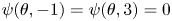 $\psi (\theta,-1)=\psi (\theta,3)=0$ for all
  $\theta$. The unsteady system is evolved using a second-order backward difference (BDF2) time stepper (Ascher & Petzold Reference Ascher and Petzold1998) with time step
  $\mathrm {{d}t=10^{-4}}$. The elements in the
  $\theta$-directions are uniformly distributed, and the elements in the
  $y$-direction are non-uniformly distributed via a
  $\tanh$ function over
  $y\in [-1,3]$, such that half the elements are restricted to
  $y<-0.93$ and
  $y>2.93$, allowing for higher resolutions near the zero boundaries. The initial condition
  $\psi (\theta,y,0)$ is uniform with a small
  $\tanh$ correction to match the boundary conditions, and satisfies
  $\int _0^{2{\rm \pi} }\int _{-1}^3\psi _0(\theta,y,0)\,\mathrm {d} y\,\mathrm {d}\theta =8{\rm \pi}$.
3. Results
First, we study different physical boundary-interaction scenarios and determine appropriate continuum boundary conditions for capturing their dynamics (§ 3.1). We consider three types of wall interactions: specular reflection  $\mathcal {S}$ (§ 3.1.1); uniform random reflection
  $\mathcal {R}$ (§ 3.1.2); and absorbing boundary
  $\mathcal {A}$ (§ 3.1.3). For each case we find a corresponding continuum model. Then, we consider different bulk flow and particle properties and analyse how they affect cells approaching boundaries (§ 3.2) for the diffusive case (§ 3.2.1) and for the deterministic case (§ 3.2.2).
3.1. Boundary conditions
3.1.1. Specular reflection (boundary condition $\mathcal {S}$)

In this section we investigate the IBM with specular reflection  $\mathcal {S}$ and consider how it compares with a continuum doubly periodic Poiseuille flow,
  $\mathcal {DP}$. In the literature, double Poiseuille flows have been used for studying low and high shear trapping in the bulk flow of bacterial suspensions to circumvent the problem of explicitly implementing a boundary (Vennamneni et al. Reference Vennamneni, Nambiar and Subramanian2020), but there has been no comparison between the wall dynamics of specular reflection IBMs and continuum doubly periodic Poiseuille models.
Consider the case of a bounded, stochastic IBM with boundary condition  $\mathcal {S}$ (figure 2b) with
  $Pe=10^1$,
  $Pe_T=10^6$,
  $\nu =0.04$ and
  $\beta =0.99$, quantifying rotational diffusion, translational diffusion, velocity ratios and cell shape, respectively. The lowest trajectory in figure 2 highlights a cell trajectory which starts oriented downstream near the bottom wall (
 $\theta =2{\rm \pi} )$, reorients rapidly until it is aligned upstream (
 $\theta ={\rm \pi} )$, and enters a region of accumulation (the yellow region) closer to the bottom wall. Once there, the cell moves up and down in the channel due to translational diffusion effects with orientation approximately parallel to the flow direction. If no longer pointed parallel to the flow direction due to rotational diffusion and shear effects, it reorients rapidly again. The extended alignment with the flow direction is a result of the shape-dependent Jeffery orbits, in which local sheared flows cause particle rotation and straining. In addition to reorientation due to Jeffery orbits, there exist additional variations of cell trajectories in orientation space because rotational diffusion can counteract or enhance reorientations and thereby affect the spreading of trajectories in physical space.
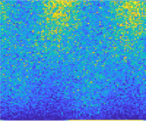
The macroscopic areas of accumulation in phase space  $(\theta,y)$ are dependent on both the shape and the motility of the swimmers. The thickness and location of the areas of accumulation are dependent on the balance between deterministic shape-dependent effects and diffusion effects. In figure 3(a–c) we consider probability distribution functions of cell distributions for
  $\beta =0.99$,
  $\nu =0.04$ and
  $Pe_T=10^6.$ For high diffusion (see figure 3a), there exist two regions of accumulation and two regions of depletion of equal widths at each wall, resulting from strong, continuous mixing of cells. With increasing
  $Pe$ (see figure 3b,c), the relative diffusive effects decrease and deterministic effects begin to dominate. Due to the nature of Jeffery orbits (which have been described earlier), more cells will be parallel to the flow direction. The reduced diffusion ensures decreased spreading in orientation space, thereby leading to thinner areas of accumulation in the
  $(\theta,y)$ phase space. For very weak rotational diffusion
  $Pe=10^4$ (see figure 3c) the areas of accumulation become very thin and cells swim away from the walls leading to peaks of accumulation at
  $(\theta,y)=({\rm \pi}, \pm 0.5)$, in agreement with observations by Rusconi et al. (Reference Rusconi, Guasto and Stocker2014) and Zöttl & Stark (Reference Zöttl and Stark2013).

Figure 3. Comparison of snapshots of bivariate probability density distributions  $\psi$, as obtained for converged IBMs with (a–c) specular wall reflections
  $\mathcal {S}$ and (d–f) equilibrium probability density distributions for doubly periodic continuum models
  $\mathcal {DP}$:
  $\beta =0.99$,
  $\nu =0.04$ and
  $Pe_T=10^6$; (a,d)
  $Pe=1$, (b,e)
  $Pe=10^2$ and (c,f)
  $Pe=10^4$.
Next, we consider the continuum doubly periodic Poiseuille flow, that serves as a potential alternative for capturing the bulk flow in the bounded domain. Consider the finite element model with a doubly periodic flow profile as shown in figure 2(c). Comparing the lower subdomain for the finite element double Poiseuille model  $\theta \in [0,2{\rm \pi} ], y\in [-1,1]$ in figure 2(a) with the bivariate stochastic IBM distribution (figure 2b) we find similar bulk-flow dynamics with regions of cell accumulation above
  $y=-1$, at angles slightly greater than
  $\theta =0,{\rm \pi}$. Meanwhile, just below
  $y=1$, near the ‘upper wall’, there also exist two areas of accumulation of equal intensity, but of flipped geometry, for angles just below
  $\theta =2{\rm \pi}$ and
  $\theta ={\rm \pi}$. In both cases, these areas of accumulation correspond to swimmers oriented close to the horizontal, but pointing out of the wall and into the wall, respectively. When comparing the probability density distributions of the doubly periodic Poiseuille continuum model (figure 3d–f) with the IBM with specular reflection (figure 3a–c) for increasing
  $Pe$, we observe the same sharpening of accumulation areas, with the occurrence of localised peaks in both figure 3(c,f). The thickness of the areas of accumulation agree as well as the intensity of cell accumulations.
Next, we compare the cell concentration distributions of swimmers,  $n(y)$, across the channel height
  $y\in [-1,1]$ for
  $\beta =0.99$, for different values of rotational diffusion (
 $Pe=1, 10^1, 10^2,10^4$). Direct comparisons between the doubly periodic continuum model (figure 4a), a doubly periodic IBM (figure 4b),and the wall-bounded IBM with specular reflection
  $\mathcal {S}$ (figure 4c) show clear agreement in the cell concentrations and accumulations. Direct comparison between the
  $\mathcal {DP}$ continuum problem and IBM specular reflection
  $\mathcal {S}$ in figure 4(d) shows clear agreement for high
  $Pe$. Deviations between the models are only notable very close to the walls for medium
  $Pe$ where the IBM with specular reflection exhibits some cell depletion as highlighted in figure 4(d). The observed depletion is observed consistently for medium
  $Pe$, and is a result of specular reflection in the IBM. Comparing with the bivariate distribution in figures 2(b) and 3(b), we note that there is a cell depletion around
  $\theta =0$ for
  $y=-1$ and
  $\theta ={\rm \pi}$ at
  $y=1$ that is not captured by the continuum model. A contributing factor to this cell depletion is finite time stepping. Due to the finite nature of time steps in the SDE problem, cell trajectories can drift, leading to reduced cells around
  $\theta =0$ for
  $y=-1$ and
  $\theta ={\rm \pi}$ at
  $y=1$.No matter how small the time-step error, cumulative effects can lead to considerable errors over long times, hence producing less accurate local distributions as time evolves (see Appendix B for details of cell trajectory drift in deterministic problems and at medium Péclet numbers). For high
  $Pe$ the migration of cells towards the channel centre due to low shear trapping (Vennamneni et al. Reference Vennamneni, Nambiar and Subramanian2020) results in low cell concentrations at the wall. The effects of drifting due to finite time step sizes are small because there are low cell concentrations at the wall. Meanwhile, for low
  $Pe$, the high rotational diffusion results in model-dependent depletion being largely counteracted. However, it is important to note that while the finite time step can contribute to the localised depletion, the observed depletion for medium
  $Pe$ is significantly larger than those expected from compounded cell drifting. This suggests that the regions of cell depletion are inherent features of specular reflection at medium
  $Pe$. While the origin of these large dips are still unclear, their appearance only for a range of medium Péclet shows that there exists a balance between advective time scales and rotational diffusion time scales over which a stable layer of depletion occurs. Overall, we note that the observed structures and positions of cell distributions obtained across all three models are in good agreement in the bulk flow across the studied range of rotational diffusions, capturing centreline cell depletion measured for medium-to-high rotational effects (low-to-medium Péclet numbers) as observed in experiments (Rusconi et al. Reference Rusconi, Guasto and Stocker2014) as well as numerical and analytical studies (Bearon & Hazel Reference Bearon and Hazel2015; Vennamneni et al. Reference Vennamneni, Nambiar and Subramanian2020). The strong agreement in the bulk flow and near the walls for high and low
  $Pe$ suggests that the doubly periodic Poiseuille continuum model might be a sensible modification for capturing the cell distributions of elongated swimmers undergoing specular reflection at high and low diffusion effects, but not for medium
  $Pe$ near the wall.

Figure 4. Cell number density distributions for (a) the continuum model distribution with doubly periodic Poiseuille flow; (b) IBM with doubly periodic Poiseuille flow; (c) the IBM distribution with specular reflection boundary condition; and (d) the direct comparison between IBM with specular reflection boundary condition (dashed lines) and the distributions of the continuum model with doubly periodic Poiseuille flow (solid lines). For shape parameters  $\beta =0.99$ with
  $Pe=10^4$ (blue),
  $Pe=10^2$ (red),
  $Pe=10^1$ (yellow) and
  $Pe=1$ (purple).
While the cell concentration distribution  $n(y)$ tells us about the agreement in the relationship between the three models in terms of cell accumulation for
  $\beta =0.99$, it does not allow for any insight into the orientations of the swimmers at or near the walls. In figure 5 we compare the probability density distributions
  $\psi (\theta,y)$ for the doubly periodic Poiseuille flow continuum model (figure 5a–c), the IBM double periodic Poiseuille flow case (figure 5d–f) and the IBM specular reflection model (figure 5g–i), for Péclet numbers
  $Pe=1$ (figure 5a,d,g),
  $Pe=10^1$ (figure 5b,e,h) and
  $Pe=10^2$ (figure 5c,f,i). For direct comparison between the doubly Poiseuille models we plot the distributions at
  $y=-1$, given by solid lines, for shape parameter
  $\beta =0, 0.5, 0.99$. To provide a comparison between the continuum model and the IBM we need to account for the numerical cell depletion. To capture near-wall cell distributions, we plot the probability distributions just beyond the model-induced depletion area near the walls at
  $y_{near}=-1+3\epsilon$ for
  $\epsilon =0.04$, as dashed lines.

Figure 5. Comparing the distributions at the wall for varying  $Pe$ and
  $\beta$, between the doubly periodic continuum model and the wall-bounded specular reflection IBM for
  $\nu =0.04$ and
  $\beta =0, 0.5, 0.99$. The probability distributions
  $\psi$ at
  $y=-1$ (solid lines) and
  $y=-1+3\epsilon$ (dashed lines) for the double Poiseuille continuum model, for (a)
  $Pe=1$ (
 $n_\theta =100$,
  $n_y=500$); (b)
  $Pe=10^1$ (
 $n_\theta =200$,
  $n_y=500$); and (c)
  $Pe=10^2$ (
 $n_\theta =400$,
  $n_y=200$). The probability distributions
  $\psi$ at
  $y=-1$ for the doubly periodic Poiseuille IBM, for (d)
  $Pe=1$; (e)
  $Pe=10^1$; and (f)
  $Pe=10^2$. The probability distributions
  $\psi$ near the bottom wall
  $y=-1+3\epsilon$ for the wall-bounded IBM with specular reflection, for (g)
  $Pe=1$; (h)
  $Pe=10^1$; and (i)
  $Pe=10^2$. The dotted line in (h) corresponds to the probability distribution near the bottom wall at
  $y=-1+\epsilon$ for the wall-bounded IBM with specular reflection for
  $Pe=10^1$ and
  $\beta =0.99$.
We note that across the continuum models for spherical swimmers ( $\beta =0$ given by the blue lines), the orientation distribution is constant, indicating that surface interactions in the absence of hydrodynamic wall interactions, show no preferential orientation. This uniformity is due to spherical swimmers undergoing a constant rate of reorientation in sheared flows as spheres have no preferred direction. This is confirmed further by both IBM models, which do not display any preferential wall interactions orientations for all considered orientational Péclet numbers.
For the case of high rotational diffusion,  $Pe=1$, we note that all distributions for non-spherical swimmers peak at approximately
  $\theta ={\rm \pi} /4$ and
  $\theta =5{\rm \pi} /4$ (with troughs at approximately
  $\theta =3{\rm \pi} /4$ and
  $\theta =7{\rm \pi} /4$) across all models, with peak concentrations increasing with cell elongation. As the rotational diffusion decreases, corresponding to an increase in the rotational Péclet number, the peaks shift towards
  $\theta =0$ and
  $\theta = {\rm \pi}$ for all
  $\beta$, with peaks clearly sharpening for the case of
  $\beta =0.99$. For
  $\beta =0.5$ there is a non-monotonic change in
  $\psi _{peak}$, shifting from
  $\psi _{peak}\approx 1.3$ to
  $\psi _{peak}\approx 1.5$ to
  $\psi _{peak}\approx 1$ for
  $Pe=1, 10^1,10^2$, respectively. The shift in peaks has a two-fold origin: the relative roles of advection and swimming (deterministic effects) versus diffusion effects, and the shift in the bulk cell distributions due to high- and low-shear trapping. In the aforementioned case, as rotational diffusion effects decrease (increase from
  $Pe=1$ to
  $Pe=10^1$) the decrease in randomness leads to decreased orientational spreading and sharper peaks. The slight elongation of cells (
 $\beta =0.5$) results in cells spending more time aligned parallel to the flow direction. Meanwhile high- and low-shear trapping are phenomena observed by Vennamneni et al. (Reference Vennamneni, Nambiar and Subramanian2020), where high-shear trapping refers to the shape and rotational diffusion-dependent migration of cells towards channel walls, and similarly, low-shear trapping refers to the migration of swimmers towards the centreline. In our studies, both high-shear trapping and low-shear trapping are captured for
  $\beta =0.99$, as evidenced by the high-shear trapping leading the peak of the wall distribution increasing from
  $\psi _{peak}\approx 1.6$ to
  $\psi _{peak}\approx 4$ to
  $\psi _{peak}\approx 8$, for
  $Pe=1,10^1,10^2$, respectively, before a transition to low-shear trapping for
  $Pe=10^4$ in figure 4 as the cells move away from the walls.
We further compare the profiles across the different models. For a small Péclet number  $Pe=1$ (see figure 5a,g) the profiles at
  $y_{near}$ (the dashed lines) are in good agreement, with similar peak magnitudes and spreads. The IBM distributions for
  $\beta =0$ are in agreement with the doubly Poiseuille cases in figure 5(a–i). For
  $Pe=10^2$ and
  $\beta =0.99$ (figure 5c,i) the central peaks about
  $\theta ={\rm \pi}$ are of similar height. However, the central peak about
  $\theta ={\rm \pi}$ is slightly larger in the individual-based model, due to the localised depletion of the peak profile about
  $\theta =0$. The depletion of the peak is, however, minor as the rotational diffusion is sufficiently large to feed more cells into the depletion areas. It is further worth noting that at
  $Pe=10^2$ drifting in long time distributions is only significant at
  $y_{near}$ for elongated swimmers as the deterministic trajectories of elongated swimmers point more sharply away from the wall about
  $\theta =0$, leading to an increased radius of depletion compared with more spherical swimmers. Running IBM double Poiseuille simulations, as shown in figure 5(d–f) corresponding to
  $Pe=1,10^1,10^2$, we find that the probability distributions at
  $y=-1$ (solid lines) match with those obtained from the continuum model figure 5(a–c) after sufficiently long runtimes.
Comparing the specular reflection IBM with the continuum double Poiseuille models, we find a good fit in the probability distributions at  $y=-1+3\epsilon$ within the studied range of rotational diffusion strengths and elongations. We see that all peak height and width distributions are in agreement, with only a slight discrepancy between the peak heights at
  $Pe=10^2$ for
  $\beta =0.99$ in the specular reflection IBM, indicating larger spatial depletion at high
  $Pe$ for strong elongation.
The good fit between the specular reflection IBM and the doubly periodic Poiseuille continuum model for small and large  $Pe$ raises the question of how the doubly periodic model's symmetry constraints on
  $\psi$ and
  ${\partial \psi }/{\partial y}$ at
  $y=\pm 1$ relate to the literature (Jiang & Chen Reference Jiang and Chen2019, Reference Jiang and Chen2020). From figure 5(a–f), we note that for the periodic boundary cases, the equilibrium cell probability density distributions satisfy
  $\psi (\theta,\pm 1)=\psi (\theta +{\rm \pi},\pm 1)$ and that the derivatives satisfy
  $({\partial \psi }/{\partial y})(\theta,\pm 1)=-({\partial \psi }/{\partial y})(\theta +{\rm \pi},\pm 1)$. Note that it is not necessary for all the derivatives to be identically zero for all
  $\theta$. The combination of these symmetries ensures the flux condition
  $J_\theta (\pm 1)=-J_{\theta +{\rm \pi} }(\pm 1)$, the integral no-flux at the boundary and impermeability are all satisfied for the equilibrium problem. We note that this observed boundary flux relationship for the
  $DP$ model differs from Jiang & Chen (Reference Jiang and Chen2019, Reference Jiang and Chen2021), in which for their time-evolving continuum models with non-uniform initial condition, the flux condition itself was prescribed to be specular, by imposing the equivalent of
  $J_\theta (\pm 1)=-J_{2{\rm \pi} -\theta }(\pm 1)$, through the constraints
  $\psi (\theta,\pm 1)=\psi (2{\rm \pi} -\theta,\pm 1)$ and
  $({\partial \psi }/{\partial y})(\theta,\pm 1)=-({\partial \psi }/{\partial y})(2{\rm \pi} -\theta,\pm 1)$, in our coordinate system. This was then compared with a double Poiseuille with half-channel flows being in the same direction which has a jump in shear at
  $y=\pm 1$. We note that the imposed conditions in Jiang & Chen (Reference Jiang and Chen2019) satisfy the no-flux condition, and though the bulk results are consistent across Jiang & Chen (Reference Jiang and Chen2019) and our model, the imposed wall behaviours in Jiang & Chen (Reference Jiang and Chen2019) differ from those that emerge in our continuum model. Recalling, that our continuum model does not capture the dip at the wall from the specular IBM for medium
  $Pe$, we consider the probability distribution
  $\psi$ even closer to the bottom wall at
  $y=-1+\epsilon$ for
  $\beta =0.99$ and
  $Pe=10^1$ in figure 5(h) as given by the dotted line. We find that the distribution can change significantly across the small length scale of
  $2\epsilon$, from a
  ${\rm \pi}$-periodic distribution to a
  ${\rm \pi}$-symmetric probability distribution. This wall symmetry is consistent with the model developed by Jiang & Chen. Furthermore, it has been confirmed via private communications that the alternate model used in Jiang & Chen (Reference Jiang and Chen2019, Reference Jiang and Chen2021) captures the near-wall dips that the
  $\mathcal {DP}$ model does not capture, suggesting it is a more appropriate boundary condition for medium
  $Pe$ and potentially more appropriate overall. As both systems satisfy the no-flux and the expected bulk flow dynamics, this reinforces the importance and sensitivity in the choice of boundary conditions when developing continuum models for active suspension dynamics.
While we have shown that the dynamics from specular reflection are well captured by a continuum approximation with doubly periodic boundary conditions, we know that microswimmers’ surface interactions are not perfect specular reflections with a variety of factors affecting surface scattering (Kantsler et al. Reference Kantsler, Dunkel, Polin and Goldstein2013; Théry et al. Reference Théry, Wang, Dvoriashyna, Eloy, Elias and Lauga2021). A swimmer near the wall may remain oriented upstream for a significant period of time, it may attach to the surface, or it may leave the surface at varying outgoing angles which may be independent of the incident angles. Keeping this in mind, we consider the effects of two further wall-interaction models: perfectly random reflections (§ 3.1.2) and perfect absorption (§ 3.1.3)
3.1.2. Random reflections (boundary condition $\mathcal {R}$)

In this section, we consider the effects of random uniform reflections at the boundaries on the equilibrium dynamics of microswimmer suspensions. Consider the model with random uniform reflection out of the wall as defined by (2.18), such that the angle of reflection of each swimmer is independent of the angle of incidence. In figure 6(a–c), we see the bivariate cell probability density distribution  $\psi$ for
  $\beta =0.99$ for varying rotational Péclet numbers. By inspection, the bulk flow distributions are similar to those found via the doubly periodic continuum model and the specular reflection IBM, with areas of cell accumulations which sharpen with increased
  $Pe$. However, from figure 6(c) we clearly note the appearance of secondary peaks at
  $( \theta,y)=(0,\pm 0.93)$ for
  $Pe=10^4$, and also note smaller peaks occurring at
  $(\theta, y)=(0.13, -0.94)$ and
  $(\theta,y)=(2{\rm \pi} -0.13, 0.94)$ for
  $Pe=10^2$ (figure 6b). No clear peak is visible for
  $Pe=1,$ as rotational effects dominate deterministic secondary structures. We note further, that the upper bound of the aforementioned secondary peaks are bounded at
  $\theta =0$ by the cusp of the deterministic trajectory originating from
  $y=-1$ and
  $\theta ={\rm \pi}$.

Figure 6. Comparison of snapshots of bivariate probability density distributions  $\psi$, as obtained converged IBMs with random wall reflections (a–c), to equilibrium probability density distributions for continuum models with constant boundary condition:
  $Pe=1$ (a,d),
  $Pe=10^2$ (b,e); and
  $Pe=10^4$ (c,f).
Noting that the secondary peaks are wholly introduced by the uniform reflective conditions, we seek to determine the appropriate continuum model boundary condition to obtain the corresponding bulk dynamics. To capture the uniformity of reflection, and lack of orientation preference upon reflection, we consider a continuum model with a constant Dirichlet wall-boundary condition (constraint  $\mathcal {D}_C$ introduced in § 2.2.2) such that
  $\psi$ is the same constant on both walls. From figure 6(d–f) we find secondary peaks occurring at the same points in phase space, indicating that slightly away from the wall there is an enhanced number of cells swimming downstream.
To further confirm the suitability of comparing the IBM with random uniform reflection with the continuum model with a constant Dirichlet boundary condition, we consider the cell number density distributions in figure 7. We compare the distribution obtained from both models in figure 7(c) for  $\beta =0.99$. We find that both profiles for
  $Pe=10^4$ (the blue lines) have the same primary peaks about
  $y=\pm 0.5$ as observed for the IBM with specular reflection, but we also get a significant peak in density about
  $y=\pm 0.93$ in both figures. We further note that in both the continuum and IBM models the minimum cell densities occur at
  $y\approx \pm 0.85$. While there are discrepancies in the size of the secondary peaks found near the wall via the IBM, we find that their size is limited by the finite time steps. Too large time steps result in cells drifting away from the secondary peaks. We find that there is a computational trade off in the total runtime required to capture the macroscopic effects (such as the peaks and troughs) and the smallness of time steps required to capture the slim secondary peaks. This drift-dependent reduction in the peak is especially prominent for the case of
  $Pe=10^4$ where diffusive effects are weak. For this case, the slim secondary peaks are highly susceptible to compounded drift effects as the peaks occur just below a separatrix that for deterministic trajectories would separate cells that would always interact with the wall and those that cannot. In this case, compounded time-step dependent drifts are large enough that they can push cells out of a region that would allow for cells to interact with the wall. This ultimately leads to some cells depleting from the secondary peak to the nearest trough of cell accumulation and to the primary peaks.

Figure 7. Cell density distributions for (a) IBM with uniform random wall reflection; (b) the distribution of continuum model with constant wall distribution; and (c) the direct comparison between IBM with uniform random wall reflection (dashed lines) and the distributions of the continuum model with constant wall distribution (solid lines). For shape parameters  $\beta =0.99$ with:
  $Pe=10^4$ (blue);
  $Pe=10^2$ (red);
  $Pe=10^1$ (yellow); and
  $Pe=1$ (purple).
Comparing figures 7(a) and 7(b) we similarly find the distributions for  $Pe=10^2$ to be a good match with the previous models (figure 4) except at the locations of the secondary peaks. Finally, there is good agreement between the IBM and continuum models for
  $Pe=1$, suggesting that overall the uniform reflection boundary is most accurate for low
  $Pe$.
$Pe$.
3.1.3. Perfectly absorbing boundary (boundary condition $\mathcal {A}$)

Our final boundary condition of interest is the case of perfect wall attachment  $\mathcal {A}$, i.e. any swimmer that encounters the wall will adhere to it. For ease of comparing the effect on the bulk dynamics we allow for specular reflection at the top wall (
 $y=1$) while enforcing a perfectly absorbing bottom wall, such that cell trajectories are terminated upon contact with the bottom wall (
 $y=-1$). It is worth noting that given the presence of diffusive effects, given sufficient time, all cells will attach to the bottom wall. Let us begin by considering a snapshot of the bivariate probability density distributions
  $\psi$ at time
  $T=600$ for the stochastic IBM. In figure 8(a) (
 $\beta =0.99$ and
  $Pe=1$), the distributions show clear depletion near the bottom wall, as all cells that have been able to encounter the bottom have attached. In figure 8(b) (for
  $Pe=10^2$) fewer cells are captured by the bottom wall by time
  $T=600$, however, there is a clear depletion, and the accumulation band in the bottom-half contains approximately 75 % the number of cells compared with their upper-half channel specular-reflecting counterparts. Finally, we consider figure 8(c) (for
  $Pe=10^4$). The yellow line is a separatrix for fully deterministic cell trajectories, where all cells below the line must interact with the wall, and all cells above will not in the absence of diffusion. We find that figure 8(c) mainly has depletion of cells originating below the separatrix, as cell diffusion is very small. For the absorbing boundary condition, there exists a non-zero flux because cells are leaving the bulk flow at the boundaries. In figure 8(g) we consider the fraction of cells absorbed at the bottom wall in time, which measures the cumulative cell flux at the wall. We find that the highest absorption rate is at the start when the cell density near the surface is at its highest. As the rate of cell absorption decreases continuously in time, the integral of the flux must change in time too. We also note see that by
  $T_{sim}=600$ approximately 30 %, 12 % and 5 % of total cells were absorbed at the bottom wall for
  $Pe=1, 10^2,10^4$, respectively, with absorption plateauing earliest for
  $Pe=10^4$ (yellow line). Therefore, higher diffusion effects yield higher rates of wall absorption for extended times.

Figure 8. Snapshots of the effects of a perfectly absorbing wall condition for different  $Pe$ at the bottom wall for an IBM (with dynamics at the top wall prescribed by specular reflection) on the bulk dynamics (a–c) at
  $T_{sim}=600$ and on normalised wall orientation probability distributions for
  $\beta =0.99$ (d–f) for runtimes
  $T_{sim}=50, 100,600$. The yellow line in (c) is a separatrix between fully deterministic trajectories which interact with the bottom wall and those that do not. In figures (d–f), the black dashed lines correspond to wall distributions for
  $\beta =0.99$ as calculated by the accumulation index (see § 3.2.2). Here: (a,d)
  $Pe=1$; (b,e)
  $Pe=10^2$; and (c,f)
  $Pe=10^4$; (g) time evolution of the fraction of cells absorbed by the bottom wall.
In figure 8(d–f), we consider the normalised orientation distributions of the cells which have been absorbed at the bottom wall. In figure 8(d) we find that in the presence of high diffusion, the wall-encounter probability distributions are wide, centred about  $\theta _{peak}\approx 21{\rm \pi} /16$, and the distributions remain unchanged for
  $T=50,100, 600$. For
  $Pe=10^2$ in figure 8(e), the peak near
  $\theta ={\rm \pi}$ continuously increases in time. This is due to a localised increase in the number of swimmers crossing the separatrix (from figure 8c) with time. The rotational diffusion is sufficiently weak that deterministic effects dominate and cells are quickly captured by the absorbing condition just above
  $\theta ={\rm \pi}$. Finally, for figure 8(f), we note a similar increase in the peak near
  $\theta ={\rm \pi}$. In fact, across figure 8(d–f), we find that the peak orientations at which absorptions occurs shifts from
  $\theta _{peak}\approx 21{\rm \pi} /16$ towards
  $\theta _{peak}={\rm \pi}$ with decreasing rotational diffusion. The difference in distribution for increasing Péclet number is a result of swimming and fluid advection dominating diffusion effects. The role of diffusion effects on cell interactions with walls will be studied in more detail in § 3.2.
We compare these results with the time evolving continuum model where we model the perfectly absorbing wall at  $y=-1$ with Dirichlet boundary condition
  $\mathcal {D}_0$ (see § 2.2.2 for details), and use the double Poiseuille profile to capture the reflective boundary condition at
  $y=1$. Note that as the continuum formulation imposes the constraint
  $\psi (y=-1, \theta,t)=0$ for all times, the continuum model cannot provide wall probability distributions comparable to figure 8. In figure 9 we compare the early time evolution of cells near the absorbing boundary using the continuum model with boundary condition
  $\mathcal {D}_0$ and stochastic boundary condition
  $\mathcal {A}$. At
  $t=0$, the stochastic system is initially uniformly distributed (see figure 9b), and the continuum model (figure 9a) has a uniform distribution everywhere except at the very thin boundary layer as defined in § 2.2.2. By
  $t=0.4$, it is clear from figure 9(c,d) that cells near the wall oriented into the wall with
  ${\rm \pi} <\theta <2{\rm \pi}$ move to the bottom wall, and those with orientations
  $0<\theta <{\rm \pi}$ swim away from the bottom wall, leaving an area of depletion. Across both models, with increasing time (figure 9e,f), the depletion area grows, emanating into the bulk domain from
  $0\leq \theta <{\rm \pi}$ as cells continue to be absorbed at
  $y=-1$ and
  ${\rm \pi} \leq \theta <2{\rm \pi}$. This persists despite the emergence of the macroscopic areas of accumulation sharpening in time. In figure 9(g,h), we see the time evolution of the cell concentration distributions for absorbing boundaries at different instants in time (see also supplementary movie 1). The concentration profiles capture the cell depletion away from the wall across both models. The depletion front (the location in
  $y$ at which we see sharp dip in cell concentration
  $n(y)$) moves into the bulk at comparable rates across the IBM and continuum models in figure 9(g,h). While the macroscopic areas of accumulation are already visibly beginning to form (see figure 9a–f) it is worth noting that in the time-evolving cell concentration profiles the cell distributions are still uniform near the wall aside from the region of cell depletion due to the absorption boundary condition. This stands in contrast to the cell equilibrium profiles for other boundary conditions (see figures 4 and 7) where there are greater spatial variations in cell concentration across
  $y$. This highlights the existence of a faster time scale of interest, which will be discussed further in § 3.2.2.

Figure 9. Early time evolution near the bottom boundary of a double Poiseuille absorbing boundary continuum model (a,c,e,g), and the stochastic IBM with specular reflection upper boundary and perfectly absorbing lower boundary (b,d,f,h), for  $\nu =0.04, \beta =0.99, Pe=10^4, Pe_T=10^6.$ Here:
  $T_{sim}=0$ (a,b);
  $T_{sim}=0.4$ (c,d); and
  $T_{sim}=0.8~$(e,f). Cell concentration
  $n(y)$ evolution near the lower wall for the continuum model with boundary condition
  $\mathcal {D}_0$ (g) and the IBM with absorbing boundary condition
  $\mathcal {A}$ (h).
3.2. Bulk flow dynamics effects on wall approach
In this section we analyse how the underlying bulk flow dynamics of swimmers of different shapes in sheared fluids impact their orientations at wall-approach in the  $\theta$–
 $y$ space. This is of particular interest as individual swimmer dynamics inform how suspensions interact with the walls, and sheds insights into why swimmers of different geometries are more likely to interact with walls at different preferred orientations, thereby affecting their likelihood of wall attachment and biofilm formation.
3.2.1. Diffusive wall approach
From the perfectly absorbing IBM (§ 3.1.3) we know that as time evolves the orientation of the cells as they interact with boundaries evolves (see figure 8d–f). The time evolution and spread of orientations at the point of wall interaction is shown to be diffusion dependent. We can analyse the extent of diffusion dependence by considering two regions of cell origin. If cells are initially uniformly distributed in the phase space, in the deterministic case we can clearly divide the cells in the phase space into two regions with respect to the yellow deterministic streamline in figure 8(c). We call the area of interactions (below the yellow line) ‘Region 1’, and the area above ‘Region 2’. In the absence of diffusion, only Region 1 cells interact with the walls. However, with increasing diffusion, larger quantities of microswimmers cross the deterministic streamlines, and more cells from Region 2 interact with the walls. The shift in interactions is captured in figure 10 for fixed IBM runtime  $T_{sim}=600$ through stacked probability distributions, where the total number of wall interactions across 51 bins are normalised to 1. For the case of
  $Pe=10^4$ with
  $\beta =0.99$, the orientation distribution peaks tend towards
  $\theta \rightarrow {\rm \pi}$ as
  $\beta \rightarrow 1$ (see figure 10c). This means that there is increased upstream alignment with elongation. From figure 10(d) we find that in this low rotational diffusion case, over 80 % of all wall interactions originate from Region 1, and this percentage decreases monotonically with
  $Pe$, irrespective of swimmer shape. An increase in rotational diffusivity, corresponding to
  $Pe=1$ (figure 10a) shifts the peak of the distribution to
  $\theta _{peak}\approx 21{\rm \pi} /16$.

Figure 10. Stacked probability distribution of angle of incidence for particles striking the lower wall ( $y=-1$), for
  $\nu =0.04$ and
  $Pe_T=10^{6}$. The blue distribution corresponds to particles which are expected to strike the wall in the absence of diffusive effects (originating in Region 1), and the red, correspond to particles that would not strike the bottom wall in the absence of diffusive effects (originating in Region 2). The overall envelope characterises the distribution of cells striking the bottom wall and integrates to 1. For
  $\beta =0.99$, (a)
  $Pe=1$, (b)
  $Pe=10^2$ and (c)
  $Pe=10^4$. (d) Ratio of cell–wall interactions with cells originating in Region 1 to total cell–wall interactions, for varying
  $\beta$ and Péclet numbers.
3.2.2. Deterministic wall approach and underlying dynamics
To further understand what happens when there is an absorbing wall we develop a novel accumulation index to capture the orientation for the fully deterministic case. To analyse shape effects on wall interactions we consider the deterministic problem, in which we keep the purely deterministic drift term and remove diffusion dynamics, such that
 \begin{gather} \displaystyle{\frac{{\mathrm{d}y}}{{\mathrm{d}t}}}=\nu\sin\theta, \end{gather}
 \begin{gather}\displaystyle{\frac{{\mathrm{d}\theta}}{{\mathrm{d}t}}}=y(1-\beta\cos2\theta). \end{gather}
From this, we derive constants of motion for the dynamics (similar to Zöttl & Stark (Reference Zöttl and Stark2013)), by eliminating time dependence and solving
 \begin{equation} \displaystyle{\frac{{\mathrm{d}y}}{{\mathrm{d}\theta}}}=\dfrac{\displaystyle{\frac{{\mathrm{d}y}}{{\mathrm{d}t}}}}{\displaystyle{\frac{{\mathrm{d}\theta}}{{\mathrm{d}t}}}}=\dfrac{\nu\sin\theta}{y(2-\beta\cos2\theta)}. \end{equation}
Integrating, we find constants of motion,  $H$, with
  $y,\theta, \beta$ and
  $\nu$ dependence, such that
 \begin{equation} H=\dfrac{y^2}{2\nu}+ \dfrac{1}{\sqrt{2\beta(1+\beta)}}\mathrm{arctanh}\left(\sqrt{\frac{2\beta}{1+\beta}}\cos\theta\right)+{C}, \end{equation}
where  $C$ is a constant dependent on particle initial conditions
  $(\theta _0, y_0)$. From this we derive the trajectories
  $y(\theta ;H,\beta,\nu )$ in phase space
  $\theta$–
 $y$, for any particle with initial condition
  $(\theta _0, y_0)$ and corresponding constant of motion
  $H$:
$H$:
 \begin{equation} y(\theta;H,\beta,\nu)=\sqrt{ {2\nu} \left(H-\dfrac{1}{\sqrt{2\beta(1+\beta)}}\mathrm{arctanh}\left(\sqrt{\frac{2\beta}{1+\beta}}\cos\theta \right)\right)}. \end{equation}
 From the trajectories we extract information regarding the expected wall interactions and trajectory times, and develop a novel accumulation index determining the distribution of expected wall interactions in the case of a uniformly seeded domain. Example trajectories are shown in figure 11(b) for  $\nu =0.04$, where
  $\beta =0$ and
  $\beta =0.99$. The shape of the trajectories themselves are dependent upon the elongation of the swimmers as highlighted in figure 11(b,c), where the black lines correspond to spherical swimmers (
 $\beta =0$), and the red dash–dotted lines correspond to
  $\beta =0.99$. Elongated swimmers undergo increasing strain effects, such that swimmers spend extended times oriented with the flow direction (
 $\theta =0,{\rm \pi}$). With increased elongation, the reorientation in phase space
  $({\partial y}/{\partial \theta })$ steepens about
  $\theta =0$ and
  $\theta ={\rm \pi}$, thus leading to a change in total area enclosed by trajectories through
  $\theta ={\rm \pi}, y=\pm 1$ and the cell trajectories upon wall approach.

Figure 11. Deterministic dynamics and the accumulation index. (a) Schematic of the accumulation index highlighting the area of phase space (blue) from which cells will interact with the bottom wall over orientation space  $\delta \theta$. The cell trajectories are shown via arrows; (b) streamlines at constants of motion for
  $\nu =0.04$,
  $\beta =0,0.99$ (solid black and dash–dotted red, respectively); (c) streamlines at constants of motion for
  $\nu =0.1$,
  $\beta =0, 0.99$ (solid black and dash–dotted red, respectively); (d) accumulation index (proportion of initially uniformly distributed cells in the phase space that are incident upon the bottom wall at angles
  $\theta$) for
  $\beta =0, 0.5, 0.99$, for
  $\nu =0.04$; (e) distribution of wall interactions with absorbing boundary conditions (solid lines) for
  $Pe=10^4$ for
  $\beta =0,0.5,0.99$ with
  $T_{sim}=5,6,$ and 50, respectively, and the corresponding accumulation index distributions (dashed lines) and (f) proportion of total area of phase space incident on the bottom wall
  $\int _0^{2{\rm \pi} }A_I(\theta ;\beta,\nu )\,\mathrm {d}\theta$ as a function of shape,
  $\beta$, for various swimming speeds,
  $\nu$.
Supposing there is an initial, uniform distribution over the entire phase plane  $\theta \times y\in [0,2{\rm \pi} )\times [-1,1]$, the accumulation index,
  $A_I$, is defined as
 \begin{equation} \int^{\theta+\delta\theta}_\theta A_I(\theta') \,\mathrm{d}\theta'=\frac{I_W(\theta,\theta+\delta\theta)}{N}, \end{equation}
where  $I_W(\theta,\theta +\delta \theta )$ is the total number of swimmers that interact with the bottom wall at
  $y=-1$ with orientations ranging in
  $[\theta, \theta +\delta \theta ]$ (see schematic in figure 11a), and
  $N$ is the total number of swimmers. The accumulation indices for orientations of incidence captured in figure 11(d) correspond to the velocity ratio
  $\nu =0.04$. For a fixed centreline flow velocity, the increased accumulation index for
  $\nu =0.1$ results from the increased swimming velocity
  $V_s$ enabling swimmers to traverse larger vertical distances prior to shear-induced reorientation. This, in turn, allows larger proportions of swimmers in an initially uniformly distributed domain to interact with the walls.
Further points of interest include the orientation  $\theta _{peak}$ at which maximal wall interactions occur. In the accumulation index (figure 11d) there is a shift in the peak interaction orientation
  $\theta _{peak}$ from approximately
  $\theta _{peak}\approx 21{\rm \pi} /16$ to
  $\theta _{peak}\approx {\rm \pi}$, with cell elongation. We find similar shape-based shifts in peak wall-interaction orientation with the absorbing boundary condition in figure 11(e).
The absorbing boundary condition distributions are shown to be in agreement with the accumulation index in the case of small rotational diffusion for shape dependent simulation runtimes  $T_{sim}$. We consider the role of swimmer shape for wall interactions as elongation affects swimming trajectories in sheared flows, especially in linearly varying shear flows. Trajectories, in turn, affect the time it takes for cells with specific initial positions and orientations to swim and rotate before cells encounter the walls. We find that the accumulation index captures the wall interactions in short runtimes only, as the clear shape-dependent shift in peak interaction orientations (figure 11e) disappears for sufficiently long runtimes, highlighting the transience of the accumulation index distribution. In figure 11(f), the total proportion of swimmers which interact with the bottom wall
  $\int _0^{2{\rm \pi} }A_I(\theta )\,\mathrm {d}\theta$ are shown for a range of shape factors and velocity ratios. For small swimming velocities, for swimmers of all considered shape factors, only a small proportion of swimmers are expected to interact with the lower wall. The proportion of wall interactions increases monotonically with swimming velocity, and increases fastest for
  $\beta >0.9$, with over 70 % of swimmers interacting with the bottom wall for
  $\nu >0.3$.
While swimmer shape affects the orientations at which swimmers are most likely to interact with the bottom wall we find that all particle trajectories are not of equal time duration. While separate identical particles on the same trajectories will have the same orbit duration in the deterministic problem, identical particles on different trajectories will have different closed-loop orbits in phase space and with different orbit durations. In figure 12, the colour maps highlight the time taken for a trajectory starting at position  $(\theta _0, y_0)$ to terminate at the bottom wall (i.e. at
  $y=-1, \theta \in [{\rm \pi}, 2{\rm \pi} ]$) via an absorbing wall boundary condition. The longest trajectories have durations ranging from
  $T\approx 6$, for
  $\beta =0$, to
  $T\approx 45$, for
  $\beta =0.99$, indicating that slender, elongated cells can take over seven times longer to complete a single full orbit, compared with spherical cells. This indicates, that strongly elongated particles have over seven times fewer opportunities for wall interactions over the fixed time interval of the faster orbit. Although a larger proportion of cells are likely to come into contact with walls at orientation
  $\theta _{peak}$ (as in figure 11d), the particles initially oriented about
  $\theta ={\rm \pi}$ have the longest closed loop trajectories and consequent orbit durations, while cells about
  $\theta =0$ have the shortest closed loop trajectories and corresponding orbit times. When considering a Lagrangian perspective, this acts as a limiting factor for the number of wall interactions per interaction orientation. The number of orbits that a particle can undergo over a fixed simulation runtime
  $T_{sim}$ is of biological interest, as it affects the probability of biofilm formation due to increased opportunities for cell attachment. Finally, we note that the accumulation index captures the deterministic limit of the perfectly absorbing boundary
  $\mathcal {A}$ (as shown in figure 11e) for runtimes corresponding to the longest closed-loop orbit durations calculated for each cell shape in figure 12.

Figure 12. Shape dependence of time taken for trajectories beginning at  $(\theta _0, y_0)$ to reach an absorbing wall condition at
  $y=-1$,
  $\theta \in [{\rm \pi},2{\rm \pi} )$. From this we can extrapolate the total number of wall interactions by swimmers in the ‘trapped’ domain over a fixed total runtime. For
  $\nu =0.04$, (a)
  $\beta =0$ and (b)
  $\beta =0.99$.
4. Conclusions
Using a finite element framework for continuum distributions of dilute suspensions of microswimmers we have studied the coupled relationship between the bulk flow cell dynamics and the boundary dynamics. We find that in order to capture the dynamics of different individual-based wall dynamics (specular reflection, uniform random reflection, absorbing boundaries), it is necessary to be cautious in the choice of boundary constraints for continuum model approximations. We find that a doubly periodic Poiseuille continuum approximation yields a good equilibrium approximation for IBM microswimmer dynamics in a wall-bounded Poiseuille flow with specular reflection for the case of high and low  $Pe$. We find that this continuum model effectively captures the macroscopic suspension distributions such as peaks of accumulation and cell depletion at the walls due to low-shear trapping in
  $y{-}\theta$ phase space. This is especially noteworthy as this offers justification for the use of doubly periodic Poiseuille flow models like Vennamneni et al. (Reference Vennamneni, Nambiar and Subramanian2020) to capture simple bounded domains with a reflective wall condition for high and low
  $Pe$. However, the doubly periodic Poiseuille flow model fails to capture dips in cell accumulation very close to walls for medium
  $Pe$. In these regions, alternate continuum models as prescribed by Jiang & Chen (Reference Jiang and Chen2019) are better approximations of specular reflection. Comparing our model with the models in Jiang & Chen (Reference Jiang and Chen2019) also highlights that the observed dips are due to specular reflection and not purely a result of shear-induced trapping. We also find that a constant boundary approximation in the equilibrium continuum model yields good agreement with an IBM with random reflections capturing additional secondary peaks of cell accumulation near the walls. For these models, we find that the uniform reflection boundary is most accurate for low to medium
  $Pe$, outside the limit where time-step sizes influence cell drifts from the secondary peaks. It is important to note that both results highlight that there exist clear limiting cases for the use of different continuum models and that the use of continuum approximations for dilute microswimmer suspensions must be made carefully. Given that cumulative effects of time-step errors are a common problem in Hamiltonian systems, a potential avenue for future research lies in studying the deterministic system from a Hamiltonian perspective to determine if there exist any symplectic integrators for the system that minimise numerical drifting. This could allow for the uncoupling of time-step effects and the inherent cell drifts at the walls due to the balance of advection and diffusion effects. Meanwhile, as the long-term limit of an absorbing boundary condition is all diffusing cells being attached to the wall, we developed a time-evolving continuum model with a zero Dirichlet boundary condition restricted to shorter simulation runtimes
  $T_{sim}<1$ due to computational costs. This model effectively captures the evolution of near-wall distributions due to wall absorption, and we have quantified the time and diffusion dependence of wall absorption for elongated particles.
The shape of the swimmers and rotational diffusion experienced by the swimmers is shown to significantly affect the orientation distributions. From a Eulerian perspective, there are no preferred cell orientations for spherical cells, while more elongated swimmers exhibit a clear preference for orientation upstream and downstream. This preference has smallest orientational spread for  $\beta =0.99$, for which the distributions are most peaked at angles just above
  $\theta =\{0,{\rm \pi} \}$ (i.e. pointing downstream and out of the bottom wall and pointing upstream and into the bottom wall), with approximately 40 % of cells being shown to interact with the walls with incidence angles
  $\theta \in [{\rm \pi} -0.25,{\rm \pi} +0.5]$. From a Lagrangian perspective, this is due to elongated swimmers spending over 60 % of their orbits aligned with the flow (
 $|\theta -{\rm \pi} |<0.1$ and
  $|\theta -2{\rm \pi} |<0.1$). On decreasing the rotational Péclet number,
  $Pe$, the spread of maximum wall incidence shifts from
  $\theta _{peak}={\rm \pi}$ to
  $\theta _{peak}\approx 21{\rm \pi} /16$ as diffusion dominates deterministic dynamics. For the case of an absorbing boundary condition, when decreasing the rotational diffusion, the wall-incidence distributions tend towards the distributions as captured by the novel accumulation index based on deterministic trajectories for runtimes corresponding to shape-dependent orbits, highlighting the importance of bulk flow swimmer trajectories on wall-interaction distributions.
The deterministic dynamics of individual trajectory dynamics in the phase plane  $\theta$–
 $y$ capture the shift in peak orientation distribution from
  $\theta _{peak}\approx 21{\rm \pi} /16$ to
  $\theta _{peak}={\rm \pi}$ for spherical to highly elongated swimmers via the accumulation index. The perpendicular approach of spherical swimmers towards surfaces and the parallel approach of elongated swimmers towards walls, have been observed for both Chlamydomonas (Buchner et al. Reference Buchner, Muller, Mehmood and Tam2021) and bacteria (Berke et al. Reference Berke, Turner, Berg and Lauga2008), respectively, in experiments and numerical studies which include hydrodynamic interactions. Our results suggest that the orientational preferences are influenced by the fundamental bulk behaviours of differently shaped swimmers.
We find that in the absence of diffusion, elongated particles take over seven times as long before interacting with the wall compared with a spherical swimmer. It is possible that elongated swimmers, therefore, must maximise each opportunity they have near the wall. Once near a wall, elongation leads to increased resistance to random Brownian rotation allowing swimmers to remain oriented parallel to flows for longer periods which improves their chemotactic sampling accuracy. Additionally, longer periods of alignment with walls allow for longer periods of mechanosensing, which increases the chances of surface attachment being initiated.
While we have considered multiple idealised wall interaction models, true biological wall interactions do not follow pin-ball dynamics, uniformly random reflections or perfect absorption, especially due to hydrodynamic interactions. In the literature, there is ongoing study into how individual swimmers interact with surfaces in the absence of flows, and even then swimmers are shown to reorient due to hydrodynamic forces. One of the nuances picked up by the accumulation index is that the bulk flow dynamics affect the likelihood of how cells approach the wall. For actual accumulation, this is also dependent on the attachment mechanisms of different swimmers, and attachment rates which are not accounted for here. Ideally, future models will combine the models with hydrodynamic interactions. For microswimmers in nature, there exist further variables which affect the likelihood of attachment and reorientation like pili attachment location (Proft & Baker Reference Proft and Baker2009; Jain et al. Reference Jain, Behrens, Kaever and Kazmierczak2012; Melville & Craig Reference Melville and Craig2013), chemical signals (Wadhams & Armitage Reference Wadhams and Armitage2004), hydrodynamic stresses (Boyle & Lappin-Scott Reference Boyle and Lappin-Scott2006; Conrad & Poling-Skutvik Reference Conrad and Poling-Skutvik2018) and cell deformability (Yoshida & Onoe Reference Yoshida and Onoe2020). Further experimental data regarding pili, and observed attachment rates at different cell orientations are required to refine the models to specific swimmer types and to draw further conclusions regarding the likelihood and speed of initial biofilm formation.
Supplementary movie
Supplementary movie is available at https://doi.org/10.1017/jfm.2023.897.
Acknowledgements
We thank the oomph-lib group for various discussions on continuum modelling. We are grateful to the referees of this paper for their insightful and constructive feedback. We are especially grateful to the reviewer who did calculations as part of their review.
Funding
We thank the UKRI for support through the grant EP/S033211/1 Shape, shear, search & strife; mathematical models of bacteria.
Declaration of interests
The authors report no conflict of interest.
Data access statement
All data and codes supporting this study are provided as supplementary information accompanying this paper at https://doi.org/10.17638/datacat.liverpool.ac.uk/2488.
Appendix A. Cell trajectories
The effect of rotational diffusion in  $x$–
$x$– $y$ space is highlighted in figure 1(c), where we neglect translational diffusion for simplicity and the IBM is augmented with an
  $x$-direction advection term such that
  $\boldsymbol {X}_t=(y(t), \theta (t), x(t))$:
 \begin{gather} \boldsymbol{\mu}(\theta,y, t)=\boldsymbol{\dot{X}}_t= \begin{pmatrix} \nu\sin\theta\\ y(1-\beta\cos2\theta) \\\hline1-y^2+\nu\cos\theta \end{pmatrix}, \end{gather}
 \begin{gather}\boldsymbol{\sigma}(\theta,y,t)=\left(\begin{array}{c c|c} \sqrt{\dfrac{2}{{Pe}_T}} & 0 & 0\\ 0 & \sqrt{\dfrac{2}{Pe}} & 0\\\hline 0 & 0 & 0 \end{array}\right). \end{gather}
Appendix B. The IBM with specular reflection: origin of the wall depletion region
For the case of the stochastic individual-based model, regions of accumulation occur in the  $\theta$–
 $y$ phase space, as observed for the doubly periodic Poiseuille flow and the wall-bounded formulation in § 3.1.1. However, in the case of the wall-bounded distribution with specular reflection at the walls, a drop in cell accumulation occurs around
  $\theta =0$ at
  $y=-1$, and
  $\theta =2{\rm \pi}$ at
  $y=1$ which increases with increased runtime. While the origin of this dip for specular reflection is not fully understood, their appearance only for a range of medium Péclet shows that there exists a balance between advective time scales and rotational diffusion time scales over which a stable layer of depletion occurs. When diffusive and advective effects are comparable they can combine to effectively remove cells from near-wall regions. However, if diffusion is low, cells do not move away; and if advection is low, cells do not get carried away.
The depletion is further compounded by a time-stepping effect that partially contributes to the drop in local cell density. The contributing factor lies in the discrete nature of the numerical method.
To illustrate this, consider the case of a purely deterministic system such that the cells must all follow predetermined trajectories. However, as time is discretised the time steps are of finite size. As shown in the schematic in figure 13(f), if a swimmer (the blue particle) begins on a deterministic trajectory given by the dotted blue line, due to discrete step sizes, the swimmer will gradually drift farther from the continuous trajectory with consecutive steps. This effect is compounded when the last step in the orbit (see the red particle on the right) undergoes specular reflection (the red particle on the left) to a position firmly outside its previous deterministic trajectory. With each cycle of reflection, the particle moves farther from  $\theta =0$, and contributes to local cell depletion. In a fully deterministic case for
  $\beta =0.99$, over a runtime
  $T=600$, we have found a 50 % cell depletion in a radius
  $r_\epsilon (=0.08)$ about
  $(\theta,y)=(0,-1)$, when increasing the step size from
  $\mathrm {d}t=10^{-3}$ to
  $\mathrm {d}t=0.1$ as seen in figure 13(a,b).

Figure 13. Figures to highlight the sensitivity of the IBM to finite time steps, and how these affect the observed boundary interactions. (a–e) The IBM Poiseuille flow, for  $\beta =0.99$,
  $\nu =0.04$. Purely deterministic IBM for
  $T_{sim}=600$ near bottom wall in (a,b), with (a)
  ${\rm d}t=10^{-3}$ and (b)
  ${\rm d}t=0.1$. (c–e) The IBM Poiseuille flow, for
  $\beta =0.99$,
  $\nu =0.04$,
  $Pe=10^1$,
  $Pe_T=10^6$, for
  $T_{sim}=600$ near bottom wall in (c,d), (c)
  ${\rm d}t=0.01$ and (d)
  ${\rm d}t=1$. (e) Cell density distribution
  $n(y)$ for diffusive case (
 $Pe=10^1$ and
  $Pe_T=10^6$) for
  ${\rm d}t=1$ (blue line) and
  ${\rm d}t=0.01$ (red line). (f) Schematic of deterministic trajectory of a particle at bottom wall in continuous time (blue dotted line) highlighting the trajectory deviation for particles of finite time step. Red particle on the right overshoots the wall, and is reflected to the red particle on the left.
In the diffusive case for  $\beta =0.99$ with
  $Pe=10^1$ and
  $Pe_T=10^6$, over a runtime
  $T=600$, we find enhanced cell depletion about
  $(\theta,y)=(0,-1)$, when increasing the step size from
  $\mathrm {d}t=0.01$ to
  $\mathrm {d}t=1$ as seen in figure 13(c,d). In this case, at
  $T=600$, we have found a 20 % cell depletion in a radius of
  $r_\epsilon$ about
  $(\theta,y)=(0.2,-1)$. While decreasing the time step size does not completely remove the cell depletion at the wall (see figure 13e), it does decrease it.


 Open access