


1. Introduction
Oceanic internal gravity waves, which are generated mainly by winds near the ocean surface or tidal flow over bottom topographies, are thought to provide a large amount of energy to sustain the ocean mixing when they break and dissipate (see e.g. Munk & Wunsch Reference Munk and Wunsch1998; St. Laurent & Garrett Reference St. Laurent and Garrett2002; Kunze & Llewellyn Smith Reference Kunze and Llewellyn Smith2004; Wunsch & Ferrari Reference Wunsch and Ferrari2004; Lamb Reference Lamb2014; Sarkar & Scotti Reference Sarkar and Scotti2017). Ocean observations have shown that although some of the waves are trapped in their generation sites and hence dissipate locally (Aucan et al. Reference Aucan, Merrifield, Luther and Flament2006; Carter & Gregg Reference Carter and Gregg2006; Lee et al. Reference Lee, Sanford, Kunze, Nash, Merrifield and Holloway2006; Levine & Boyd Reference Levine and Boyd2006; Klymak, Pinkel & Rainville Reference Klymak, Pinkel and Rainville2008; Johnston et al. Reference Johnston, Rudnick, Carter, Todd and Cole2011; Nikurashin & Legg Reference Nikurashin and Legg2011), the majority of them can radiate to far away places (Ray & Mitchum Reference Ray and Mitchum1996; Alford Reference Alford2003; Alford & Zhao Reference Alford and Zhao2007; Nash et al. Reference Nash, Alford, Kunze, Martini and Kelley2007; Kunze et al. Reference Kunze, MacKay, McPhee-Shaw, Morrice, Girton and Terker2012). These radiated waves will be largely dissipated when interacting with different kinds of ocean features such as continental slopes and seamounts (Eriksen Reference Eriksen1982; Nash et al. Reference Nash, Kunze, Toole and Schmitt2004; Klymak et al. Reference Klymak, Moum, Nash, Kunze, Girton, Carter, Lee, Sanford and Gregg2006; Zhao, Alford & Mackinnon Reference Zhao, Alford and Mackinnon2010; Alford et al. Reference Alford2011; Martini et al. Reference Martini, Alford, Kunze, Kelly and Nash2011). To better understand the internal wave dissipation and its effects on the ocean mixing, many studies have been performed to simulate and determine quantitatively the wave–topography interactions, and one of the most studied cases is the reflection or scattering of incident internal waves upon the sloping topography.
When an internal wave beam propagates in a uniformly stratified fluid, the angle of its group velocity vector with respect to the horizontal,  $\alpha$, depends only on the wave frequency $\omega$, if the effect of the Earth's rotation is neglected. The relation between $\alpha$, $\omega$ and the buoyancy frequency $N$ is given by (Sutherland Reference Sutherland2010)
 \begin{equation} \tan\alpha=\sqrt{\frac{\omega^{2}}{N^{2}-\omega^{2}}}. \end{equation}
Owing to such a property, an internal wave maintains its angle after scattering or reflection upon a slope, which can lead to much higher wavenumber and energy density, causing the instabilities and dissipation. Moreover, the overlap between the incident and reflected wave near the topography can also enhance significantly the nonlinear effects, which results in mean flow and harmonics. These physical phenomena can be influenced by several parameters, for example, the criticality (usually defined as the ratio of the topography slope to wave characteristic slope), the properties of the incident wave such as its amplitude, the shape or relative height of the topography, and the stratification of ambient fluid. Previous studies have explored thoroughly how the wave scattering depends on these control parameters (see e.g. Cacchione & Wunsch Reference Cacchione and Wunsch1974; Thorpe & Haines Reference Thorpe and Haines1987; Gilbert & Garrett Reference Gilbert and Garrett1989; Ivey & Nokes Reference Ivey and Nokes1989; Taylor Reference Taylor1993; Ivey, Winters & De Silva Reference Ivey, Winters and De Silva2000; Müller & Liu Reference Müller and Liu2000a,Reference Müller and Liub; Legg & Adcroft Reference Legg and Adcroft2003; Gostiaux et al. Reference Gostiaux, Dauxois, Didelle, Sommeria and Viboud2006; Scotti Reference Scotti2011; Rodenborn et al. Reference Rodenborn, Kiefer, Zhang and Swinney2011; Chalamalla et al. Reference Chalamalla, Gayen, Scotti and Sarkar2013; Hall, Huthnance & Williams Reference Hall, Huthnance and Williams2013; Legg Reference Legg2014; Arthur, Koseff & Fringer Reference Arthur, Koseff and Fringer2017; Nazarian & Legg Reference Nazarian and Legg2017a,Reference Nazarian and Leggb; Sarkar & Scotti Reference Sarkar and Scotti2017). However, the impact from another significant property, the roughness of the slope surface, has not been investigated systematically.
There are a number of previous studies that examine the role of surface roughness on wave scattering; all of them are theoretical. The first was by Longuet-Higgins (Reference Longuet-Higgins1969), who found that quite small-scale irregularities can completely alter the reflecting properties of a surface, and he also elucidated the impacts of different kinds of periodic surface roughnesses on wave transmission. A more quantitative study was shown by Mied & Dugan (Reference Mied and Dugan1976), and they calculated the energy redistribution of the wave scattered by a sinusoidally corrugated surface. Thorpe (Reference Thorpe2001) was the first to use a configuration with superimposed roughness elements on a sloping topography, and studied the scattering of an incident internal wave on such a topography. This work was further improved by Legg (Reference Legg2004), who incorporated the Coriolis effect. Later findings by Nakamura & Awaji (Reference Nakamura and Awaji2009) indicate that the surface roughness can also change the frequency of the incident wave under some conditions. The above theoretical models have shed some light on the effects of surface roughness on wave scattering. However, there still exist some aspects that need to be explored, one of which is that the viscous effect was not incorporated in these models, and hence a major puzzle remains, i.e. how is the dissipation of wave energy affected by the surface roughness? The main purpose of the present work is to answer such a question through a laboratory study.
In this paper, we perform a laboratory experiment to investigate the scattering, energy dissipation and mean flow induced by the internal gravity wave incident upon slopes with different surface roughness. For completeness, we examine the role of criticality, while the impact from the amplitude of the incident wave is also illustrated. The remainder of this paper is organized as follows. The experimental apparatus with a novel design, the measurement techniques and the parameter space are introduced in § 2. The main results and discussions are shown in § 3, which is divided into four subsections. The structure of the generated wave in our system is presented in § 3.1. The fields of kinetic energy and wave dissipation near the topography are shown in § 3.2. The profiles of the averaged dissipation rate and kinetic energy are presented in § 3.3. The mean flow field induced by the nonlinear effect is shown in § 3.4. We summarize our findings and conclude in § 4.
2. Experimental apparatus and methods
As shown in figure 1, the experiments were performed in a box of rectangular shape with length  $L$, width $W$, and height $H$ equal to $80\times 20 \times 20$ (cm), respectively. The working fluid that fills the box is deionized and degassed water. The top and bottom plates of the box are made of copper, with their surfaces electroplated with nickel and then chromium, while the side wall of the box is constructed by four transparent Plexiglas plates of thickness 2 cm. The top plate is heated by eight embedded heaters, and the heating power is controlled by a high-stability power supply; the bottom plate is cooled by a regulated refrigerated recirculator. For more details on the design of these plates, we refer to Xia, Sun & Zhou (Reference Xia, Sun and Zhou2003).

Figure 1. Schematic drawing of the experimental apparatus.
In this experiment, the top and bottom temperatures of the box were fixed at  $32.5 \,^{\circ }{\rm C}$ and $11.5\,^{\circ }{\rm C}$, respectively, thus the working fluid is stably stratified, with the strength of stratification being controlled by the temperature difference across the box. The surrounding temperature, controlled by two high-performance air conditioners, was set equal to the mean temperature of the box, i.e. $22.0\,^{\circ }{\rm C}$. Comparing with the traditional approach, in which saline water is used to make a stably stratified fluid layer by the two-tank method (Fortuin Reference Fortuin1960), our method has three main advantages. First, the generated stratification may be closer to that in the ocean, since the temperature, rather than salinity, has the greatest effect on density change in the ocean (Webb Reference Webb2019). Second, once the stable stratification is established, we can perform wave field measurements at any time without the need to reproduce the stratification. Third, as the stratification is determined solely by the temperature distribution, it can be measured easily by scanning the temperature profile with a thermistor attached to a movable rod. In this experiment, we scan the vertical temperature profile with a step size 5 mm. The equation that is used to convert the temperature of water $T$ at different vertical positions to its density $\rho$ is the Kell (Reference Kell1975) formulation
 \begin{equation} \rho=\frac{a_1+a_2T-a_3\times 10^{{-}3}T^{2}-a_4\times 10^{{-}6}T^{3}+a_5\times 10^{{-}9}T^{4}-a_6\times 10^{{-}12}T^{5}}{1+a_7\times 10^{{-}3}T}, \end{equation}
where  $a_1=999.83952$, $a_2=16.945176$, $a_3=7.9870401$, $a_4=46.170461$, $a_5=105.56302$, $a_6=280.54253$ and $a_7=16.897850$. The local buoyancy frequency is then obtained as
 \begin{equation} N(z)=\sqrt{-\frac{g}{\rho(z)}\,\frac{ {\rm d}\rho(z) }{{\rm d}z}}, \end{equation}
where  $g$ is the gravitational acceleration, and $z$ is the height relative to the bottom plate.
The quasi-two-dimensional internal gravity waves were generated by a smooth cylinder (19 cm in length and 5 cm in diameter), connected to a linear motor (model:  ${\rm P}01\text {-}37\times 120/20\times 100\text {-}{\rm C}$, LinMot) that was set to oscillate periodically. The motion of the cylinder, which determines the dynamics of the generated internal wave, can be described by
 \begin{equation} Z(t)=A\cos(\omega t)+Z_0-A, \end{equation}
where  $Z$ and $Z_0$ represent the vertical displacement and the initial vertical position of the generator relative to the bottom plate, while $A$ and $\omega$ are the oscillating amplitude and frequency, respectively. A set of slopes was used in the experiment to model the sloping topographies in the oceans. Each of the slopes consists of a thin acrylic plate (19 cm in length, 19 cm in width, and 0.3 cm in thickness) with certain surface roughness, and two cylindrical acrylic rods (9.5 cm in height and 1 cm in diameter) that were used to support one end of the acrylic plate, with the other end resting on the bottom plate of the box. Such a design can minimize the influence of the added topographies on thermal stratification.
In the present study, the excited internal waves can propagate towards four directions. For simplicity, only the lower left wave beam, which interacts with the slope, is marked in figure 1 by two green wavy lines. The other three wave beams, undergoing one or several reflections at the top or bottom plates, will be absorbed by two foam filters (indicated by black rectangles in figure 1) with thickness 2 cm, which were placed at the left and right ends of the tank. There is a vertical slit at the middle of the right foam filter so that the laser sheet can pass through.
The internal wave fields were measured by the particle image velocimetry (PIV) technique (Adrian Reference Adrian1991). The polyamide spheres ( $20\ \mathrm {\mu }{\rm m}$ in diameter and $1.03\ {\rm g}\ {\rm cm}^{-3}$ in density) were selected as seeding particles. A continuous laser source (PSU-H-LED, MGL-H-532-400 mW) as well as some optics were used to produce a laser sheet to illuminate the seeding particles, and the flow field was recorded by a charge-coupled device (CCD) with $2048\times 2048$ (pixel) resolution. The sampling rate was 2 Hz or 4 Hz, depending on the wave velocity, and the recording time is more than 40 wave periods for each measurement. The recorded raw images were processed by PIV calculation software (DPIV-2010) to obtain two-dimensional velocity maps. For most of the measurements (except for that used to examine the generated wave structure), the number of grid points (the calculated vectors) within the region in which we are interested is about $120\times 60$, and the spatial resolution of the PIV measurement, i.e. the distance between the adjacent grids, is 1.7 mm. As the density of the seeding particles is slightly larger than that of the water (see figure 3a), it is necessary to test the impact from the sink of the particles on the measured flow field. We took a PIV measurement before the wave generator began to vibrate. The calculated velocities within the measuring window are almost zero, suggesting that this sedimentation effect can be neglected.
In this experiment, the buoyancy frequency within the measuring region is approximately  $0.42\ {\rm rad}\ {\rm s}^{-1}$. The angle of each sloping topography with respect to the horizontal $\beta$ is fixed at $30^{\circ }$, while the oscillating frequency $\omega$, the oscillating amplitude $A$, and the wavelength of surface roughness, or simply surface roughness, $\lambda$ on a slope, are variables. Here, $\lambda$ is defined as the ratio of the height of the roughness element $h$ to the width of its base $d$ (
$d$ ( $\lambda =h/d$, see figure 1), and $h$ is fixed at 1 cm while $d$ is varied, resulting in $\lambda$ varying from 0.25 to 1.5. For comparison, we also conducted measurements using a slope with a smooth surface ( $\lambda =0$). The rough surface designed in this study is significantly different from that in a classical theoretical study mentioned above (Thorpe Reference Thorpe2001). One of the main differences is that in Thorpe's case, the steepness of roughness relative to the slope, $S$, is supposed to be a small value ( $S\ll 1$). Here, $S=0.5hk$, with $k$ being the wavenumber of the roughness element ( $k=2{\rm \pi} /d$). In the current study, the calculated $S$ varies from 0.79 to 4.71, which is close to or larger than 1. Such a difference makes the study in Thorpe (Reference Thorpe2001) less relevant to our experiment. The wave frequency $\omega$ in the present study is varied from 0.21 to 0.32 ${\rm rad}\ {\rm s}^{-1}$, so the angle of the generated incident waves with respect to the horizontal, $\alpha$, which is calculated by (1.1), varied from $30^{\circ }$ to $50^{\circ }$. In this study, there are two kinds of criticality. One of them is the criticality of large slope, which is usually defined as $\tan (\beta )/\tan (\alpha )$. To highlight the deviation from $\alpha$ to $\beta$, a new control parameter $\gamma$, the off-criticality, is introduced, defined as $(\alpha -\beta )/\beta$, and varies from 0 to 0.67 (such a definition is close to that in Chalamalla et al. Reference Chalamalla, Gayen, Scotti and Sarkar2013). Note that $\gamma = 0$ corresponds to a critical slope, and all non-zero positive values of $\gamma$ correspond to subcritical slopes. We now turn to another kind of criticality, which is the criticality of a roughness element. Figure 2 shows a geometrical sketch of the internal waves incident on a roughness element. Here, we denote the angle between the right side of the roughness element and the horizontal as $\beta _2$, which equals $\varphi +\beta$, where $\varphi$ is the angle between the right side of the roughness element and the slope surface. The criticality of the roughness elements is usually defined as $\tan (\beta _2)/\tan (\alpha )$, which then equals $\tan (\alpha +\beta )/\tan (\alpha )$. Note that $\varphi =\arctan (2\lambda )$ (where $\lambda$ is the surface roughness and equals $h/d$) and $\alpha =\gamma \beta +\beta$. The criticality of a roughness element can be expressed as $\tan (\arctan (2\lambda )+\beta )/\tan (\gamma \beta +\beta )$. Since $\beta$ is fixed at $30^{\circ }$, we see that the criticality of a roughness element can be determined by $\lambda$ and $\gamma$, and hence is not a new independent control parameter for our system. In Appendix C, we will show that the criticality of a roughness element is not a good choice as control parameter.

Figure 2. Illustration of internal waves incident on a roughness element. The green arrows represent the incident waves, and the solid black lines constitute a roughness element superimposed on a slope. Here,  $\varphi$ is the angle between the right side of the roughness element and the slope surface, $\alpha$ is the angle of the incident waves with respect to the horizontal, and $\beta$ is the angle of the slope with respect to the horizontal. The width and height of the roughness element are denoted $d$ and $h$, respectively. For simplicity, we plot only one of the roughness elements.
The amplitude  $A$ is set from 1.5 to 6 mm. Therefore, $A/D$ varied from 0.03 to 0.12, where $D$ is the diameter of the oscillating cylinder as indicated in figure 1. As the role of the wave amplitude in wave–topography interaction is not the main focus of this study, details of dependence of the scattered wave properties on the amplitude $A$ will be illustrated in Appendix B.
3. Results and discussion
3.1. The generated wave beam in the absence of topographies
To begin with, we check the vertical density profile measured in the system, which is shown in figure 3(a). Here, the inset shows the measured temperature profile, which is used to calculate the density profile by (2.1). The buoyancy frequency  $N$ (calculated by (2.2)) is shown in figure 3(b), where there are four data sets that were measured over a period of one month. The overlap of these four data sets shows excellent stability of the established stratification. The buoyancy frequency is not uniform in the vertical direction. However, within the measuring region, indicated by the two dashed lines in figure 3(b), the buoyancy frequency is nearly constant, with mean value 0.42. As indicated by (1.1), the value of $N$ determines the upper limit of the frequency of the generated wave.

Figure 3. (a) The density profile from data set 1, which is calculated by the measured temperature profile (inset). (b) The profiles of buoyancy frequency from four data sets measured over a period of one month. The dashed lines indicate the vertical range of the measuring window.
We now examine the structure of the generated wave in our system in the absence of topographies. An example of the vector maps of the measured internal wave field is plotted in figure 4(a). Here,  $A/D=0.03$ and $\omega /N=0.21$. Also, $T$ is the length of the wave period, and $t=T/4$ is the time when the cylinder reaches the equilibrium position and moves downwards.

Figure 4. Vector maps of internal wave velocity with magnitude  $\sqrt {u^{2}+v^{2}}$ ${\rm cm}\ {\rm s}^{-1}$ coded in both colour and arrow length at $A/D=0.03$, $\omega /N=0.21$ and $t=T/4$: (a) experimental measurement; (b) theoretical prediction. The black solid line and red dashed line indicate, respectively, the perpendicular and parallel directions of the energy propagation of the waves.
Assuming that the boundary condition at the surface of the wave generator is free-slip, and that the variation of the excited internal wave in the across-beam direction is much larger than that in the along-beam direction, Hurley & Keady (Reference Hurley and Keady1997) proposed a viscous linear theory to describe the internal waves generated by a vibrating elliptic cylinder in stratified fluid of constant buoyancy frequency. Such a theory (referred to as HK theory hereafter) has been used to compare with previous experiments (Sutherland et al. Reference Sutherland, Dalziel, Hughes and Linden1999; Zhang, King & Swinney Reference Zhang, King and Swinney2007). In figure 4(b), we plot the wave field predicted by the HK theory with the same values of the parameters as in the experiment. One sees that the experimentally measured wave field shows good correspondence with that predicted by theory.
To make a more quantitative comparison, we plot the profiles of along-beam velocity (velocity in the direction of wave propagation)  $V_a$ in figure 5, which are taken across the black lines shown in figure 4. Here, $b$ represents the relative distance of the points on the black line to the centre of the line, and the minus or plus sign of $b$ means the point is located below or above the midpoint on the black line. From figures 5(a) and 5(c), we see that the experimental results can be described very well by the HK theory. In figures 5(b) and 5(d), where the wave frequency becomes larger, it can be seen that HK theory under-predicts the wave amplitude when $b$ is positive. The increase of the deviations between the experiments and the HK theory when $\omega$ increases was also found in Sutherland et al. (Reference Sutherland, Dalziel, Hughes and Linden1999). This will not be discussed further as it is not the main focus in the present study.

Figure 5. The profiles of along-beam velocity when  $t=T/4$: (a) $A/D=0.03$, $\omega /N=0.21$; (b) $A/D=0.03$, $\omega /N=0.30$; (c) $A/D=0.09$, $\omega /N=0.21$; (d) $A/D=0.09$, $\omega /N=0.30$.
Figure 6 shows the variation of the wave amplitude in the direction of the group velocity from our measurement and the prediction from the linear HK theory in a semi-logarithmic plot. One can see clearly that neither the experimental data nor the model predication follows the exponential decay described by the classical wave attenuation equation for a monochromatic wave (Lighthill Reference Lighthill1978). The figure also shows some differences between the experimental data and linear model prediction; the difference is about 10 % in the largest case. Such a deviation is also found in some previous works. For example, in Zhang et al. (Reference Zhang, King and Swinney2007), the difference between the theory and experimental data can be as large as 50 % (figure 6(d) in their paper).

Figure 6. The variation of wave amplitude in the direction of the group velocity. The data are taken at the positions indicated by the red dashed lines in figure 4.  $q$ is the coordinate along the direction of the group velocity of the waves. The origin of $q$ is the cross point of black solid lines and red dashed lines in figure 4. Note that the vertical scale in this figure is logarithmic.
3.2. Wave field near the rough slope
We now place the topography into the box and study the wave fields near the slopes with different surface roughness. The scattering of the incident internal waves can be seen clearly in figure 7, where we show the contour maps for the fields of time-averaged kinetic energy:
 \begin{equation} E =\frac{1}{t_2-t_1}\int_{t_1}^{t_2}(u^{2}/2+w^{2}/2)\,\mathrm{d} t. \end{equation}
Here,  $u$ and $w$ are the horizontal and vertical velocities, respectively, $t_1$ is a time when the flow reaches steady state, and $t_2$ is chosen such that $t_2-t_1$ is larger than at least 30 oscillating periods. For simplicity, we show only the results when $A/D=0.03$ and
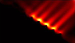
  $\gamma =0.50$. Figures 7(a) to 7(e) show that the internal waves are modulated by the surface roughness of the slope: The wave patterns exhibit light and dark stripes in the whole flow field. This is because of the constructive/destructive interference between the incident waves and the reflected waves. This effect becomes increasingly prominent as the roughness parameter $\lambda$ is increased from 0 to 0.5. As $\lambda$ becomes larger than 0.5, and the wavelength of the roughness becomes small, this kind of modulation is weakened. When $\lambda =1.5$, the wave field is very close to that in smooth surface case. One may also find that high-intensity regions of the wave are around the peak positions of the roughness elements, which is due to the energy concentration during the wave reflection. Low-intensity regions correspond to the valley positions of the roughness elements, because part of the wave is trapped near the valley and hence becomes stagnant. Moreover, figure 7 shows that the kinetic energy of an internal wave is the largest in the region very close to the surface of the topography. Surprisingly, this maximum value shows no significant dependence on $\lambda$.

Figure 7. Contour maps for the fields of time-averaged kinetic energy at different  $\lambda$ when $A/D=0.03$ and $\gamma =0.50$: (a) $\lambda =0$, (b) $\lambda =0.25$, (c) $\lambda =0.5$, (d) $\lambda =0.75$, (e) $\lambda =1.5$. The units are ${\rm cm}^{2}\ {\rm s}^{-2}$.
In figure 8, we show the fields of time-averaged dissipation rate:
 \begin{equation} \epsilon =\frac{1}{t_2-t_1}\int_{t_1}^{t_2}\varepsilon\,\mathrm{d} t, \end{equation}
where  $\varepsilon$ is the instantaneous dissipation rate of kinetic energy in two-dimensional flow (Pope Reference Pope2000):
 \begin{equation} \varepsilon=\nu\left[2\left(\frac{\partial u}{\partial x}\right)^{2}+2 \left(\frac{\partial w}{\partial z}\right)^{2}+\left(\frac{\partial u}{\partial z}+\frac{\partial w}{\partial x}\right)^{2}\right]. \end{equation}
Here,  $\nu$ is the kinematic viscosity of water. To measure the dissipation rate accurately, the Kolmogorov length scale should be resolved in the PIV measurement. However, the spatial resolution should not be too high, otherwise the measurement error increases (Tokgoz et al. Reference Tokgoz, Elsinga, Delfos and Westerweel2012). In this experiment, it is difficult to realize fully the above requirements at each grid point because of the spatial inhomogeneity, i.e. the resolution is a bit too low for some high-dissipation region, but may be a little too high for some low-dissipation region. Hence a direct comparison between the measured dissipation field in the rough surface cases and that in the smooth surface case can be only qualitative.

Figure 8. Contour maps for energy dissipation at different  $\lambda$ when $A/D=0.03$ and $\gamma =0.50$: (a) $\lambda =0$, (b) $\lambda =0.25$, (c) $\lambda =0.5$, (d) $\lambda =0.75$, (e) $\lambda =1.5$. The value of $\log _{10}\langle \epsilon \rangle _t$ is coded in colour. The units are ${\rm cm}^{2}\ {\rm s}^{-3}$.
Figures 8(a) to 8(e) show the modulation of the surface roughness on the energy dissipation of internal waves. For all cases, the energy dissipation is the largest near the slope, and the maximum energy dissipation in the smooth surface case is even larger than that in the rough surface case. On the other hand, in the roughness case, the region of intense dissipation seems to be less localized and is extended beyond the vicinity of the surface. This results in the distribution of dissipation rate in the rough cases being more uniform in space. Again, the dissipation field at  $\lambda =1.5$ is found to be close to that in the smooth surface case.
3.3. Profiles of dissipation rate and kinetic energy
To analyse quantitatively the effect of roughness on internal wave field, we plot and then examine the profiles of the averaged dissipation rate along the direction normal to the slope. We first introduce a new coordinate system shown in figure 8(b): the origin is set at halfway along the slope surface. Two variables,  $s$ and $\sigma$, represent the coordinates parallel and perpendicular to the slope surface, respectively. We then take the average of $\epsilon$ in the $s$ direction:
 \begin{equation} \langle \epsilon \rangle(\sigma)=\frac{1}{\varDelta}\int_{s_1}^{s_2} \epsilon (\sigma,s)\,\mathrm{d} s, \end{equation}
where  $s_1$ and $s_2$ are equal or close to $-l/2$ and $l/2$, respectively, in the region near the slope, $l$ being the length of the rough surface of the slope ( $l=16$ cm). Also, $\varDelta =(s_2-s_1)\xi$, where $\xi$ is the ratio of the number of the grid points outside the roughness elements to the total number of grid points at a certain $\sigma$. In the region far away from the slope, the length of the average region, i.e. $s_2-s_1$, would be smaller than $l$ due to the finite size of the measuring window, which may partly reduce the accuracy of $\langle \epsilon \rangle$. However, as most of the energy is dissipated near the slope, such a finite size effect is negligibly small in the final results. Although the measured energy dissipation may be less than accurate at some grid points, as mentioned before, we have verified that the obtained profiles of $\langle \epsilon \rangle$ are accurate and reliable (for details about the verification, please refer to Appendix A). For simplicity, we will show only the dissipation profiles that were measured with $A/D=0.03$.
In figures 9(a,b), we plot the normalized average dissipation rate  $\langle \epsilon \rangle /\epsilon _0$ versus the normalized distance normal to the slope, $\sigma /h$. Here, $\epsilon _0=A^{2}\omega ^{3}$, and $h$ is the height of the roughness element, as we said before. These figures show that the surface roughness reduces the maximum value in the dissipation profile. It is also seen that the peak width of the profiles in the rough cases is larger than that in the smooth surface case. This is consistent with the observation from figure 8 that the energy dissipation becomes less localized and is spatially more uniform when the slope surface is rough. Another feature shown in these figures is that when $\lambda \geqslant 0.50$, the energy dissipation is very weak when $\sigma$ is very close to the valley of the roughness ( $\sigma \approx 0$). A possible reason is that part of the incident wave is trapped near the valley of the roughness elements and hence become stagnant, as we said before. The results are the same for other values of $\gamma$. In figures 9(c,d), we plot the profiles of the normalized accumulated dissipation rate, $\epsilon _{T}/\epsilon _{T0}$. Here, $\epsilon _{T}$ is defined as
 \begin{equation} \epsilon_T(\sigma)=\frac{\rho W_0l}{s_2-s_1}\int_{0}^{\sigma}\int_{s_1}^{s_2} \epsilon (\sigma,s)\,\mathrm{d} s\,\mathrm{d\sigma}, \end{equation}
where  $\rho _0$ is the density of water, and $W_0$ is the width of the slope. Also, $l/(s_2-s_1)$ is the normalization factor, which is used to make the integral length in the $s$ direction remain the same at different $\sigma$, and thus can reduce the impact from the finite size of the measuring window. As (3.5) shows, $\epsilon _{T}(\sigma )$ reflects the total amount of energy dissipation in the region below a certain $\sigma$. We have $\epsilon _{T0}=\rho _0 {l_0}^{3}A^{2}\omega ^{3}$, where $l_0$ is the unit length (1 cm). Both figures 9(c) and 9(d) show that the surface roughness can also reduce the total amount of the energy dissipation, and this roughness-induced reduction shows a clear dependence on $\lambda$. When comparing figures 9(c) with 9(d), we see that the roughness-induced reduction is much more prominent at $\gamma =0.17$, suggesting that such a reduction is also highly related to the off-criticality.

Figure 9. Profiles of (a,b) the along-slope and time-averaged dissipation rates, and (c,d) the accumulated dissipation rate. For (a,c)  $\gamma =0.5$, and for (b,d) $\gamma =0.17$. Different symbols represent different roughnesses as shown in (a).
In figure 10, we examine the influence of the off-criticality on the energy dissipation, where the profiles of the averaged and accumulated dissipation rates are both shown for various values of  $\gamma$. It is found that there exists a non-zero optimal off-criticality ( $\gamma _{{optimal}}=0.17$) for energy dissipation in both the smooth and rough surface cases. Surprisingly, unlike surface roughness, the off-criticality is found to apparently have no effect on the peak width of the dissipation profile, but affects its shape only far from the slope. This suggests a weak dependence of the spatial distribution of the dissipation on off-criticality, which is confirmed further in figure 11.

Figure 10. Profiles of (a,b) the normalized average dissipation rate, and (c,d) the accumulated dissipation rate. For (a,c)  $\lambda =0$, and for (b,d) $\lambda =0.5$. Different symbols represent different off-criticality.

Figure 11. Full width at half-maximum (FWHM) of the profiles of the averaged dissipation rate versus  $\lambda$ at different $\gamma$.
In figure 11, we plot the normalized full width at half-maximum (FWHM) of the peaks in the profiles of the averaged dissipation rate versus  $\lambda$ at different $\gamma$. It is seen that the peak width of the dissipation profile indeed depends weakly on off-criticality, as the values of FWHM/ $h$ at different $\gamma$ are close. Rather, FWHM/ $h$ of the dissipation profiles is determined mainly by the surface roughness. The peak width in rough surface cases can be much larger than that in the smooth surface case, as figure 9 shows. Moreover, the peak width increases monotonically when $\lambda$ decreases from 1.50 to 0.25. Figure 11 demonstrates quantitatively that the region of intense dissipation is broadened due to the effect of surface roughness.
From both figures 9 and 10, we see that the energy dissipation accumulates rapidly in the region near the slope (except for the regions where  $\sigma$ is very close to 0 in some rough surface cases, i.e. near the valley of the roughness elements), and then accumulates very slowly in the region far from the slope. We introduce a quantity called the displacement boundary layer (DBL), which is used to separate the rapid accumulation and slow accumulation regions. The method to determine the thickness of the DBL is shown in figure 12(a). We extrapolate the linear parts of the accumulated dissipation profile both near the slope and far from the slope, and the distance from the slope at which these two extrapolating lines cross corresponds to the thickness of the DBL. We plot the thickness of the DBL ( $\delta$) versus the off-criticality $\gamma$ at different surface roughnesses $\lambda$ in figure 12(b), which shows that $\delta$ has a weak dependence on $\gamma$, and the data scatter may be due to the errors in determining the DBL thickness. The figures also show that the DBL thickness for the smooth surface is much smaller than for the rough cases. The differences between the DBL thicknesses in the smooth and rough surface cases are close to the height of the roughness element. This suggests that such differences are determined mainly by the height of the roughness element.

Figure 12. (a) Illustration of determining the thickness of the displacement boundary layer (DBL) by the slope method. (b) The thickness of the DBL versus off-criticality at different surface roughnesses.
To examine the effects of roughness on energy dissipation more completely, we plot in figure 13(a) the maximum value of the averaged dissipation  $\langle \epsilon \rangle _{max}$ in the profiles measured at all $\gamma$, versus the surface roughness $\lambda$. It is seen that for each $\gamma$, $\langle \epsilon \rangle _{max}$ first decreases and then increases with increasing $\lambda$. Except for the case with $\gamma =0$, $\langle \epsilon \rangle _{max}$ reaches a minimum at $\lambda =0.5$, where the modulation effect is most pronounced, as shown in figure 7. The ratio of $\langle \epsilon \rangle _{max}$ at $\lambda =0$ (smooth surface case) to that at $\lambda =0.5$ can be as large as $\sim$10. We also plot the total dissipation rate at $\sigma =2\delta$, namely $\epsilon _T|_{\sigma =2\delta }$, versus $\lambda$ in figure 13(c). When $\sigma$ reaches $2\delta$, the dissipation has decayed significantly and the accumulated dissipation $\epsilon _T$ increases very slowly with the distance $\sigma$, hence $\epsilon _T|_{\sigma =2\delta }$ can be used as a measure of the total energy dissipation. Although the relation between $\epsilon _T|_{\sigma =2\delta }$ and $\lambda$ is somewhat complex, a broad feature is that the surface roughness reduces $\epsilon _T|_{\sigma =2\delta }$ under most circumstances. Figure 13(c) also shows that the total energy dissipation has less dependence on $\lambda$ when compared with the maximum value in the dissipation profile. The reason is that although the surface roughness reduces the maximum value of the dissipation rate, it broadens the region of intense dissipation. The combination of these two effects reduces the dependence of the total accumulated dissipation on the surface roughness. In figures 13(b) and 13(d), we plot $\langle \epsilon \rangle _{max}$ and $\epsilon _T|_{\sigma =2\delta }$ versus off-criticality $\gamma$, respectively. It is clear that there exist an optimal off-criticality at which both $\langle \epsilon \rangle _{max}$ and $\epsilon _T|_{\sigma =2\delta }$ reach their respective maximums. This optimum off-criticality remains invariant for different surface roughnesses, and equals 0.17. It should be noted that because of the sparsity of the data, this number serves to provide only a rough measure of the true optimal value. Another feature seen from figure 13(d) is that the value of $\epsilon _T|_{\sigma =2\delta }$ for $\gamma =0$, i.e. waves with critical incidence, is the same for surfaces with different roughnesses, even for a smooth surface, which is somewhat unexpected. It would be interesting to explore the relation between the criticality of the slopes of the roughness elements (the definition of the criticality is shown in § 1) and the energy dissipation of waves. However, as already mentioned (see Appendix C for details), this criticality is not a good choice as a control parameter.

Figure 13. Maximum value in the averaged dissipation profile  $\langle \epsilon \rangle _{max}/\epsilon _0$ versus (a) roughness $\lambda$, and (b) off-criticality $\gamma$. Accumulated dissipation rate at $\sigma =2\delta$, $\epsilon _T|_{\sigma =2\delta }/\epsilon _{T0}$, versus (c) roughness $\lambda$, and (d) off-criticality $\gamma$. The symbols represent different off-criticality in (a,c), and different surface roughnesses in (b,d).
It is known that stronger flow strength usually leads to stronger energy dissipation. Thus we also investigate the relationship of wave energy to surface roughness and off-criticality. In figure 14, we plot the profiles of the normalized average kinetic energy  $\langle E \rangle /E_0$. Here, the method to obtain the time- and space-averaged kinetic energy $\langle E \rangle$ is the same as that used to obtain $\langle \epsilon \rangle$ in (3.4), and $E_0$ used for the normalization equals $A^{2}w^{2}$. From figures 14(a) and 14(b), we see that the surface roughness has little effect on the strength of the internal wave near the slope except that it shifts the peak position position by a distance roughly equal to the height $h$ of the roughness elements (1 cm). Figures 14(c) and 14(d) show that the wave energy near the slope can be affected by off-criticality. The more quantitative examination is shown in figure 15, where we plot the maximum value in the profile of averaged wave energy $\langle E \rangle _{max}/E_0$ versus surface roughness $\lambda$ in (figure 15a) and vs off-criticality $\lambda$ in (figure 15b). Indeed, the wave energy near the slope has no significant dependence on surface roughness, but is dependent only on the off-criticality. The optimum $\gamma$ equals 0.17 and is the same as that found in figures 13(b) and 13(d).

Figure 14. Profiles of the normalized averaged kinetic energy  $\langle E \rangle /E_0$ at different surface roughnesses $\lambda$, with (a) $\gamma =0.5$, and (b) $\gamma =0.17$; and at different off-criticality $\gamma$, with (c) $\lambda =0$, and (d) $\lambda =0.5$.

Figure 15. Maximum value in the averaged kinetic energy profile  $\langle E \rangle /E_0$ versus (a) roughness, and (b) off-criticality.
In some of the previous studies, critical reflection ( $\gamma =0$) has attracted most of the attention as it can result in the strongest wave energy near the slope according to the linear inviscid theory. However, the present study suggests that the strongest wave energy exists at off-criticality 0.17, not 0. In our understanding, the optimum off-criticality should be determined by two effects: the energy concentration effect, which enhances the wave energy near the slope, and the effect induced by the bottom drag, which reduces the wave energy. When the off-criticality decreases to zero, both of these effects are enhanced continuously, and their combination leads to a non-zero optimum off-criticality. In the classical theory, the viscous effect is not incorporated, hence the optimum off-criticality should be zero. The existence of non-zero optimal off-criticality is also found in other studies; e.g. Chalamalla et al. (Reference Chalamalla, Gayen, Scotti and Sarkar2013) reported that the turbulent kinetic energy can be higher for somewhat off-critical reflection compared to exactly critical reflection under certain conditions. A weakly nonlinear model (Kataoka & Akylas Reference Kataoka and Akylas2020) also shows that in some conditions, the viscous effect can be important during the wave reflection from a slope, which leads to the deviation of the optimal off-criticality from zero.
3.4. Mean flow
As mentioned in § 1, the mean flow field induced by the interaction between incident wave and topography can reflect the strength of the nonlinear effect. The previous theoretical and experimental studies have elucidated clearly the two-dimensional mean flow field near slopes with smooth surface (Thorpe & Haines Reference Thorpe and Haines1987; Grisouard Reference Grisouard2010). In this subsection, we focus on the influence of surface roughness on the mean flow field. The vector map of the mean flow velocity  $U\boldsymbol {e}_x+W\boldsymbol {e}_z$ for the smooth surface and rough surface cases are shown in figures 16(a) and 16(b), respectively. Here, $U$ and $W$ are long-time-averaged horizontal and vertical velocities, while $\boldsymbol {e}_x$ and $\boldsymbol {e}_z$ are the rightward and upward unit vectors, respectively. A comparison between these two figures clearly shows that the surface roughness changed the structure of the mean flow field: a series of vortices, of size roughly the same as the separation between the tips of roughness elements, are formed near the slope surface. In the case of a smooth surface, the direction of the mean flow is mainly parallel to the slope. However, in the rough surface case, the formation of vortices is accompanied by the enhancement of mean flow in the direction perpendicular to the slope, which is further confirmed in figures 16(c) and 16(d), where we show the contour plots of mean flow velocity in the direction perpendicular to slope surface $V_{\sigma }$. It is found that $V_{\sigma }$ in the rough surface case is much stronger than that in the smooth surface case (notice the difference in the scale bar). For comparison, we also plot the fields of the mean flow velocity in the direction parallel to slope $V_s$ in figures 16(e) and 16( f). Although the roughness elements would induce additional bottom drag force as we mentioned before, it is found that the strength of $V_s$ in the rough surface case is even slightly larger than that in the smooth surface case.

Figure 16. (a,b) Coarse-grained vector maps of the mean flow velocity  $U\boldsymbol {e}_x+V\boldsymbol {e}_z$, with the magnitude $\sqrt {U^{2}+W^{2}}$ coded in both colour and arrow length for the smooth and rough cases, respectively. (c,d) Colour-coded contour plots of mean flow velocity in the direction parallel to slope $V_s$. (e, f) Colour-coded contour plots of the mean flow velocity perpendicular to slope $V_{\sigma }$. In (a,c,e) $\lambda =0$; in (b,d, f) $\lambda =0.5$. Here, $A/D=0.09$, $\gamma =0.50$, and the units are ${\rm cm}\ {\rm s}^{-1}$.
The normalized maximum values of mean flow velocity in the direction normal to slope  $(V_{\sigma }/V_0)_{max}$ versus surface roughness $\lambda$ and off-criticality $\gamma$ are plotted in figures 17(a) and 17(b), respectively. Here, $V_0=A\omega$ is used for normalization. It can be seen that $(V_{\sigma }/V_0)_{max}$ first increases and then decreases as $\lambda$ increases continuously. Interestingly, the maximum value of ( $V_{\sigma }/V_0)_{max}$, which represents the strongest nonlinear effect, corresponds to the position $\lambda =0.5$, at which the scattering effect becomes strongest, as shown in figure 7, and $\langle \epsilon \rangle _{max}$ reaches a minimum. From figure 17(b), it is found that there also exists an optimal off-criticality ( $\gamma =0.17$) for $(V_{\sigma }/V_0)_{max}$. The existence of an optimal off-criticality for mean flow is not difficult to understand, as the wave energy near the slope is largest at that off-criticality, as shown in figure 15(b).

Figure 17. Normalized maximum value of the mean flow velocity perpendicular to slope,  $(V_{\sigma }/V_0)_{max}$, versus (a) roughness $\lambda$, and (b) off-criticality $(\alpha -\beta )/\beta$.
4. Conclusion
In this paper, we have investigated experimentally the scattering, energy dissipation and mean flow when the incident internal waves are scattered by sloping topographies with rough surfaces in a stably stratified fluid maintained by a constant temperature gradient. The surface roughness  $\lambda$ (the ratio of the height of the roughness element to the width of its base) and the off-criticality $\gamma$ (which relates directly to the wave frequency) are chosen as two main variables of the experiment, while the wave amplitude $A$ is fixed in most cases.
As a validity check of the design of our system, the quality of the generated internal wave, and the measurement techniques, we first examine the generated wave beams in the absence of the topographies in the fluid. When comparing the obtained results with a viscous linear theory developed by Hurley & Keady (Reference Hurley and Keady1997), which is a widely used linear model, it is found that the structure of the internal wave in our system can be well described by this theory. The scattering of incident wave by the surface roughness is shown in both the time-averaged kinetic energy field and the energy dissipation field. The effect of scattering enhances as  $\lambda$ increases from 0 to 0.5, and then weakens as $\lambda$ increase from 0.5 to 1.5. Moreover, the distribution of energy dissipation is found to be more uniform in the direction perpendicular to the slope when the slope surface is rough. Counter-intuitively, although the roughness elements should enhance the drag force on the surface of the slope, both the maximum value in the profile of space- and time-averaged energy dissipation, $\langle \epsilon \rangle _{max}$, and the total energy dissipation, $\epsilon _T|_{\sigma =2\delta }$, are reduced by the surface roughness under most circumstances. Nevertheless, the peak width of the dissipation profile is found to be broadened significantly in the rough surface cases, which demonstrates that the intense dissipation region can be extended by the surface roughness. The peak width is found to increase monotonically when $\lambda$ decreases from 1.50 to 0.25. Interestingly, the roughness is also found to affect strongly the mean flow field induced by wave–topography interaction. The structure of mean flow has been changed drastically by roughness: a series of vortices, of size roughly the same as the separation between the tips of roughness elements, are formed near the slope. Contrary to its role in energy dissipation, the surface roughness greatly enhances the mean flow in the direction perpendicular to the slope surface. The normalized maximum value of mean flow velocity in the direction normal to the slope, $(V_{\sigma }/V_0)_{max}$, reaches its maximum at $\lambda = 0.5$, at which the scattering becomes strongest and $\langle \epsilon \rangle _{max}$ reaches minimum.
The role played by off-criticality  $\gamma$ is examined systematically. It is observed that there exists an optimal $\gamma$ ( $=0.17$ for the present measurement resolution) for the normalized $\langle \epsilon \rangle _{max}$ and $\epsilon _T|_{\sigma =2\delta }$, which may be attributed to the strongest kinetic energy near the slope at that $\gamma$. The combination of energy concentration effect and the effect induced by bottom drag force should be responsible for the existence of this non-zero optimal off-criticality, which is different from the prediction of linear inviscid theory. Not surprisingly, the same optimal off-criticality is found in the measured mean flow field when $\lambda$ is varied. Unlike surface roughness, the off-criticality has only a small effect on the distribution of energy dissipation.
Our study suggests, under the present conditions, that the surface roughness of topography can reduce both the maximum energy dissipation and total energy dissipation. Furthermore, the surface roughness is found to broaden the region of intense dissipation. The wave-induced mean flow is also enhanced by the surface roughness. Moreover, there exists a non-zero optimal off-criticality at which the dissipation near the topography reaches maximum. In the oceans, topographies with rough surfaces are thought to be the regions where energy dissipates strongly (see e.g. Ledwell et al. Reference Ledwell, Montgomery, Polzin, St. Laurent, Schmitt and Toole2000). The present study therefore provides a new perspective on how the surface roughness on topographic features influences energy dissipation. Finally, we remark that further studies are needed to examine whether the present laboratory findings can be extended to the oceans.
Acknowledgements
The authors would like to thank S.-D. Huang for his help in the design of the experimental setup and for stimulating discussions, and thank G.-Y. Ding for technical assistance.
Funding
We gratefully acknowledge support of this work by the National Natural Science Foundation of China (grant no. 12072144), the Research Grants Council (RGC) of HKSAR (grant nos CUHK14301115 and CUHK14302317) and the Department of Science and Technology of Guangdong Province (grant no. 2019B21203001).
Declaration of interests
The authors report no conflict of interest.
Author contributions
Y.-H.H. and B.-Y.-C.C. contributed equally to this work.
Appendix A. Test the reliability of the calculated dissipation profile
Here, we test the accuracy and reliability of the profile of the time and along-slope averaged energy dissipation  $\langle \epsilon \rangle$ measured using the current spatial resolution. Figure 18 shows the profiles of the averaged dissipation measured at different resolutions (from 0.39 to 3.1 mm). For simplicity, $\lambda$ is fixed at 0.25, while $\gamma$ is fixed at 0.5. Note that to achieve high spatial resolution, the PIV measuring window in this test is limited to a small region near the slope, hence the measured dissipation profiles would be a little different from that shown in figure 9. From figures 18(a–d), it is found that all the profiles with their measuring resolutions within the range from 1.5 mm to 3 1 mm can collapse nicely onto a single curve, which means that the resolutions within this range are appropriate for measuring the dissipation profiles. The chosen spatial resolution in the present PIV measurement is 1.7 mm, thus the profiles of $\langle \epsilon \rangle$ in this study are reliable. The values and the errors of $\langle \epsilon \rangle$ at $\sigma =h$, which are the mean and standard deviation of $\langle \epsilon \rangle$ at these appropriate resolutions, are given in figure 18, and the errors are small when compared with the ratio of dissipation in the rough surface case to that in the rough surface case.

Figure 18. The profiles of time and along-slope averaged dissipation rate  $\langle \epsilon \rangle$ measured at different resolutions when $\lambda =0.25$ and $\gamma =0.5$: (a) $A/D=0.03$, (b) $A/D=0.06$, (c) $A/D=0.09$, and (d) $A/D=0.12$. Different symbols represent different resolutions, the values of which are listed to the right of (b) with the unit mm. The values and errors of $\langle \epsilon \rangle$ at $\sigma =h$ are also given.
Appendix B. Dependence on the forcing amplitude
Here, we analyse the role played by the amplitude of the incident wave in energy dissipation and mean flow. In figure 19, we plot  $\langle \epsilon \rangle$ at $\sigma =h$ versus $A^{2}$, and the data are from figure 18. It is clear that $\langle \epsilon \rangle |_{\sigma =h}$ is proportional to the square of the wave amplitude. In figure 20, we plot the maximum mean flow velocity in the direction parallel to slope $V_s(\max )$ versus $A^{2}$ at different $\gamma$. For simplicity, $\lambda$ is fixed at 0. Again, it is found that $V_s(\max )$ is proportional to $A^{2}$.

Figure 19. Plot of  $\langle \epsilon \rangle$ at $\sigma =h$ versus $A^{2}$ when $\lambda =0.25$ and $\gamma =0.5$.

Figure 20. The maximum mean flow velocity in the direction parallel to the slope  $V_s(\max )$ versus $A^2$ when $\lambda =0$.
Appendix C. Dependence on the criticality of the slopes of the roughness element
Figure 21 shows the maximum value in the averaged dissipation profile versus the criticality of the slopes of the roughness elements. The criticality is defined as  $\tan (\beta _2)/\tan (\alpha )$, where $\beta _2$ is the angle between the right side of the roughness element and the horizontal, and $\alpha$ is the angle of the incident waves. One may see that the data points in the figure are very scattered, which means that the criticality of the slopes of the roughness elements seems not to be a good choice as a control parameter in this study. We would also like to emphasize that this criticality is not a independent variable as it is determined when the values of $\lambda$ and $\gamma$ are given.

Figure 21. Maximum value in the averaged dissipation profile  $\langle \epsilon \rangle _{max}/\epsilon _0$ versus the criticality of the slopes of the roughness element. The data are taken from figure 13(a). The data in the smooth surface case are not used as there are no roughness elements.


