


1. Introduction
Capsules consisting of a liquid droplet enclosed by a thin elastic membrane are commonly encountered in nature in the form of red blood cells, fish eggs and vesicles and in numerous industrial processes. The protection and controlled release of active agents is of great importance for diverse applications in the food, cosmetic, bioengineering and medical engineering industries, among others. In medicine, encapsulation has opened the way to new treatment techniques like targeted drug/gene therapy (Bhujbal, de Vosl & Niclou Reference Bhujbal, de Vosl and Niclou2014). New-generation bioartificial organs/cells are being developed, for instance, by encapsulating islets of Langerhans to treat diabetic patients (Su et al. Reference Su, Hu, Lowe, Kaufman and Messersmith2010) or haemoglobin to create artificial blood (Li, Nickels & Palmer Reference Li, Nickels and Palmer2005).
But when placed in suspension, capsules are subjected to intense stresses from the surrounding flow, which may cause the mechanical degradation of the membrane. In vivo tests have shown that artificial blood cells could be easily damaged in circulation depending on the particle shape and deformability (Li et al. Reference Li, Nickels and Palmer2005): this example illustrates the importance of controlling rupture. Depending on the application, capsule damage is to be prevented to preserve the inner substance, or, on the contrary, fostered and directed to allow a targeted release of the encapsulated substance. This necessitates a good understanding of the capsule damage mechanisms under low-inertia flow conditions and of the parameters that control the initiation of rupture.
Very few studies have been conducted on the rupture of capsules subjected to hydrodynamic stresses. The only results that currently exist are experimental. Early experimental studies showed the possibility of wrinkling formation at low shear rates (Walter, Rehage & Leonhard Reference Walter, Rehage and Leonhard2001), which could lead to fatigue mechanisms, and of capsule burst at high shear (Chang & Olbricht Reference Chang and Olbricht1993). The results by Chang and Olbricht (Chang & Olbricht Reference Chang and Olbricht1993) were obtained on macroscopic spherical capsules, produced through interfacial polymerization. Flow-induced rupture initiated from one of the major axis tips of the deformed ellipsoidal shape of the capsule, which corresponds to the point of minimum thickness. The crack then propagated in the shear plane. Rupture of microcapsules under simple shear flow was observed by Koleva & Rehage (Reference Koleva and Rehage2012) on thin polysiloxane capsules having a high degree of crosslinking. It was reached at small deformations, indicating a brittle behaviour of the capsule membrane. Increasing the shear rate, rupture typically occurred in the central region, close to the tips of the flow vorticity axis, which correspond to the zones of maximum tension. This study corroborated the results by Husmann et al. (Reference Husmann, Rehage, Dhenin and Barthès-Biesel2005), who showed that spherical and non-spherical polysiloxane microcapsules burst at the points of maximum elastic tensions, when placed in a spinning-drop apparatus. A similar breakup mechanism has been obtained in confined environments by Abkarian et al. (Reference Abkarian, Faivre, Horton, Smistrup, Best-Popescu and Stone2008) for red blood cells flowing through a  $5\ \mathrm {\mu } \textrm {m}$ wide channel, and by Le Goff et al. (Reference Le Goff, Kaoui, Kurzawa, Haszon and Salsac2017) for artificial millimetric capsules and fish eggs trapped at a constriction within a cylindrical channel under a set pressure difference. In both studies, rupture initiated at the front of the capsule, where the tensile tension is the highest. Note that, in Le Goff et al. (Reference Le Goff, Kaoui, Kurzawa, Haszon and Salsac2017), rupture could also occur at the point of contact between the capsule and the constriction, but this mode of rupture is different, as it is induced by contact and not by deformation under flow.
What is currently lacking is a model of capsule deformation under flow, capable of assessing when and where the initiation of rupture occurs. The objective of the present study is to develop the first fluid–structure interaction model accounting for membrane damage induced on a liquid-core microcapsule subjected to a simple shear flow. We will use continuum damage mechanics (CDM) to model the initiation and growth of microdiscontinuities (microcavities and microcracks), which lead to the local initiation of macrocracking as they accumulate and coalesce. Contrary to fracture mechanics, which accounts explicitly for the inherent geometrical discontinuity and the associated boundary conditions, the microdiscontinuities are not geometrically modelled in CDM. The local average damage state due to the microdiscontinuities is instead represented by a continuum variable: the damage variable. The CDM has benefited from numerous contributions to its theoretical development (e.g. Kachanov Reference Kachanov1986; Lemaitre & Desmorat Reference Lemaitre and Desmorat2005) since the pioneering work of Kachanov (Reference Kachanov1958). It is based on the thermodynamics of irreversible processes with internal variables (Coleman & Gurtin Reference Coleman and Gurtin1967), and has been applied to model the damage mechanisms of a large spectrum of materials, from engineering materials (an overview of applications is presented in Lemaitre & Desmorat Reference Lemaitre and Desmorat2005) to biological tissues (Hokanson & Yazdani Reference Hokanson and Yazdani1997; Natali et al. Reference Natali, Pavan, Carniel, Lucisano and Taglialavoro2005; Holzapfel & Fereidoonnezhad Reference Holzapfel and Fereidoonnezhad2017). We propose to incorporate a CDM model into a fluid–structure interaction framework, in order to investigate the time evolution of damage as the capsule deforms under flow.
In this study, we focus on the damage process of a capsule under intense hydrodynamic stresses induced by an external flow over a relatively short time. Due to the short time scale of the phenomena, fatigue or creep damage models are thus not presently relevant. Previous studies have shown that microcapsules may experience ductile (Ghaemi et al. Reference Ghaemi, Philipp, Bauer, Last, Fery and Gekle2016) or brittle (Koleva & Rehage Reference Koleva and Rehage2012; Le Goff et al. Reference Le Goff, Kaoui, Kurzawa, Haszon and Salsac2017) damage depending on the material and history of loading (external thermo-mechanical stresses). We derive the damage model assuming a quasi-brittle behaviour of the capsule membrane, for which dissipation prior to cracking occurs with negligible irreversible strains (i.e. negligible plasticity). However, CDM provides a general framework: the present model will thus be straightforwardly extended to the other damage behaviours (ductile material, creep or fatigue).
After having detailed the formulation of the damage model of a capsule in infinite shear flow in § 2, we present the model discretization and numerical solver in § 3. We first investigate damage of a spherical capsule under isotropic inflation in § 4, as it provides insight into capsule damage and allows us to validate the numerical method by comparison of the results with the corresponding analytical solution. We then study damage in simple shear flow in § 5, and assess the effect that the dimensionless parameters of the model have on damage evolution and rupture initiation. We finally discuss the model and results in § 6 and analyse the potential of the model to identify the capsule membrane limit of elasticity by comparison with experiments.
2. Formulation of the problem
We consider a spherical microcapsule of radius  $a$ enclosed in an elastic envelope of very small thickness with respect to its radius. The capsule is thus modelled as a two-dimensional incompressible membrane with surface shear elastic modulus $G_s$. It is placed in an infinite shear flow of shear rate $\dot {\gamma }$. The problem is studied in the reference frame of centre $O$ and Cartesian basis $(\boldsymbol {e_x},\boldsymbol {e_y},\boldsymbol {e_z})$ corresponding to the barycentric reference frame of the capsule oriented such that the unperturbed velocity field is given by
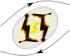
  $\boldsymbol {v}^{\infty }(\boldsymbol {x}) = \dot {\gamma } z \boldsymbol {e_x}$ (figure 1). The inner and outer fluids are the same incompressible Newtonian fluids of dynamic viscosity $\mu$ and density $\rho$. Gravitational and inertial effects being negligible due to the microscopic capsule size, the fluid–structure interaction problem is governed by only one non-dimensional parameter: the capillary number $Ca = \mu \dot {\gamma } a / G_s$, the ratio of the viscous to the elastic characteristic forces.

Figure 1. Capsule suspended in the unbounded simple shear flow.
2.1. Internal and external flows
Inertial effects being neglected, the fluid problem is governed by the Stokes equations
 \begin{equation} \textrm{div}\left(\boldsymbol{\sigma}\right)=0, \quad \textrm{div}\left(\boldsymbol{v}\right)=0, \end{equation}
where  $\boldsymbol {\sigma }$ designates the Cauchy stress tensor, $\boldsymbol {v}$ is the velocity vector and $\textrm {div}(\cdot )$ is the divergence operator. At a given point $\boldsymbol {x}$ of the membrane $S$, the boundary integral formulation of the Stokes equations gives the relationship between the velocity vector $\boldsymbol {v}$ and the stress tensor $\boldsymbol {\sigma }$ (Pozrikidis Reference Pozrikidis1992)
 \begin{equation} \forall \boldsymbol{x} \in S, \quad \boldsymbol{v}(\boldsymbol{x}) = \boldsymbol{v}^{\infty}(\boldsymbol{x}) - \frac{1}{8{\rm \pi}\mu} \int_{S} \boldsymbol{\mathsf{J}}(\boldsymbol{x}, \boldsymbol{y}) \boldsymbol{\cdot} [\kern-1pt[\boldsymbol{\sigma} ]\kern-1pt]\boldsymbol{\cdot}\boldsymbol{n}(\,\boldsymbol{y}) \,\mathrm{d}S_{\boldsymbol{y}}, \end{equation}
where  $\boldsymbol {n}$ is the unit vector normal to $S$ pointing towards the external fluid and $[\kern-1pt[ \boldsymbol {\sigma } ]\kern-1pt] \boldsymbol {\cdot }\boldsymbol {n}=(\boldsymbol {\sigma }_{ext}-\boldsymbol {\sigma }_{int})\boldsymbol {\cdot }\boldsymbol {n}$ is the stress jump across the membrane. We denote as $\boldsymbol{\mathsf{J}}$ the second-order Oseen–Burgers tensor defined by
 \begin{equation} \boldsymbol{\mathsf{J}}(\boldsymbol{x}, \boldsymbol{y}) = \dfrac{1}{r} \boldsymbol{\mathsf{1}} + \dfrac{1}{r^3} \boldsymbol{r} \otimes \boldsymbol{r}, \end{equation}
where  $\boldsymbol {r}=\boldsymbol {x} - \boldsymbol {y}$, $r=\lVert \boldsymbol {r}\rVert$ and $\boldsymbol{\mathsf{1}}$ is the identity tensor.
2.2. Wall mechanics
The capsule wall is modelled as a membrane of mid-surface  $S$. The curvilinear coordinates $(\xi _1,\xi _2)$ describe the position $\boldsymbol {x}(\xi _1,\xi _2,t)$ on $S$ in the configuration at time $t$. The position $\boldsymbol {x}(\xi _1,\xi _2,0)$ on the initial configuration $S_0$ of $S$ is noted $\boldsymbol {X}$. It is convenient to write the membrane equations in local tangent bases. In what follows, if not specified, indices written with Latin letters take values in $\{1,2,3\}$, while indices written with Greek letters are in $\{1,2\}$. The covariant basis $(\boldsymbol {a}_i)$ attached to $S$ is defined by
 \begin{equation} \boldsymbol{a}_{\alpha}=\dfrac{\partial\boldsymbol{x}}{\partial\xi_{\alpha}}, \quad \boldsymbol{a}_{3}=\dfrac{\boldsymbol{a}_{1}\times\boldsymbol{a}_{2}} {\left\lVert\boldsymbol{a}_{1}\times\boldsymbol{a}_{2}\right\rVert}. \end{equation}
The contravariant basis  $(\boldsymbol {a}^i)$ is defined by $\boldsymbol {a}_i\boldsymbol {\cdot }\boldsymbol {a}^j=\delta _i^j$, where $\delta _i^j$ designates the Kronecker symbol. On $S_0$, the covariant and contravariant bases are denoted $(\boldsymbol {A}_i)$ and $(\boldsymbol {A}^i)$, respectively. The metric tensor is $\boldsymbol{\mathsf{g}}$ on $S$ and $\boldsymbol{\mathsf{G}}$ on $S_0$. The contravariant and covariant components of $\boldsymbol{\mathsf{g}}$ are $a^{\alpha \beta }=\boldsymbol {a}^{\alpha }\boldsymbol {\cdot }\boldsymbol {a}^{\beta }$ and $a_{\alpha \beta }=\boldsymbol {a}_{\alpha }\boldsymbol {\cdot }\boldsymbol {a}_{\beta }$, respectively (similar definitions for the components $A^{\alpha \beta }$ and $A_{\alpha \beta }$ of $\boldsymbol{\mathsf{G}}$).
The wall inertia being negligible (Walter et al. Reference Walter, Salsac, Barthès-Biesel and Le Tallec2010), the motion of the membrane is governed by the local mechanical equilibrium
 \begin{equation} \forall \boldsymbol{x} \in S, \quad \boldsymbol{{\nabla}_s} \boldsymbol{\cdot} \boldsymbol{\mathsf{T}} + \boldsymbol{q} = \boldsymbol{0}, \end{equation}
where  $\boldsymbol {q}$ is the surface external load, $\boldsymbol{\mathsf{T}}$ is the tension (resultant of the internal Cauchy stress over the thickness), $\boldsymbol {{\nabla }_s} \boldsymbol {\cdot }$ is the surface divergence operator. The dynamic boundary condition imposes that
 \begin{equation} \forall \boldsymbol{x} \in S, \quad \boldsymbol{q} = [\kern-1pt[\boldsymbol{\sigma} ]\kern-1pt]\boldsymbol{\cdot}\boldsymbol{n}. \end{equation}
The weak form of the membrane equilibrium equation is obtained applying the principle of virtual work
 \begin{equation} \begin{array}{c} \text{For any virtual displacement } \boldsymbol{\hat{u}} \in H^1(S), \\ \displaystyle \int_{S} \boldsymbol{\hat{u}}\boldsymbol{\cdot}\boldsymbol{q} \, \mathrm{d}S = \int_{S} \boldsymbol{\mathsf{T}}:\boldsymbol{\varepsilon}(\boldsymbol{\hat{u}}) \, \mathrm{d}S, \end{array} \end{equation}
where  $H^1(S)$ designates the Sobolev space associated with the Lebesgue space $L^2(S)$ and $\boldsymbol {\varepsilon }(\boldsymbol {\hat {u}})$ is the symmetric part of $\boldsymbol{\mathsf{g}}\boldsymbol {\cdot }\boldsymbol {{\nabla }} \,\boldsymbol {\hat {u}}$, the tensor $\boldsymbol {{\nabla }}\,\boldsymbol {\hat {u}}$ being the gradient of $\boldsymbol {\hat {u}}$.
In terms of kinematics, the no-slip boundary condition holds on  $S$ and gives the relationship between the fluid velocity and the position $\boldsymbol {x}$ of the corresponding point of the membrane
 \begin{equation} \boldsymbol{v} = \dfrac{\textrm{d}{\kern0.07em}\boldsymbol{x}}{\textrm{d}t}. \end{equation}
2.3. Material behaviour
The model of the capsule wall behaviour is developed in the standard framework of CDM (Lemaitre & Desmorat Reference Lemaitre and Desmorat2005) to account for the progressive degradation of the membrane while staying in the field of continuum mechanics. More specifically, CDM is a branch of the thermodynamics of irreversible processes with internal variables, the focus of which is to model irreversible transformations associated with damage. The development of a damage model is thus based on four key concepts inherited from the thermodynamics of irreversible processes: state variables, state potential, damage criterion and damage evolution law. A short review of these concepts together with the details of how we developed the model are given hereafter. We specify them in the case of quasi-brittle damage which corresponds to the membrane deformation until the initiation of rupture without irreversible strains (see table 1 for a summary).
Table 1. Summary of the key ingredients of the present associated damage model.

2.3.1. State variables
We assume that the transformations of the capsule wall correspond to isothermal elastic deformation and damage. The damage variable represents the irreversible growth of microdefects in a representative volume element (RVE) (figure 2).

Figure 2. Representation of a microcapsule of mid-surface  $S$ placed in an infinite shear flow (a). Zoom on a representative volume element (RVE) containing microcavities and microcracks (b). Decomposition of the cross-section $\delta S$ of normal vector $\boldsymbol {k}$ into the effective load-bearing cross-section $\delta \tilde {S}$ and the total surface of the microdefects $\delta S_D$ (c).
To illustrate the definition of the damage variable, we consider a deformed RVE of the capsule wall containing microdefects in the form of microcavities and microcracks (figure 2). We define damage in direction  $\boldsymbol {k}$ as the surface ratio $\delta S_{D}/\delta S$, with $\delta S_{D}$ the maximum intersection of microdefects in a cross-section $\delta S$ of normal $\boldsymbol {k}$ of the RVE. The stresses on this cross-section are thus transmitted on $\delta \tilde {S} = \delta S - \delta S_{D}$. We assume that the microdefects have no preferential orientation: the $\delta S_D/\delta S$ ratio is thus independent of the direction $\boldsymbol {k}$ and corresponds to isotropic damage. The state variable is then the scalar damage variable $d$ defined as
 \begin{equation} d = \dfrac{\delta S_{D}}{\delta S} = 1 - \dfrac{\delta \tilde{S}}{\delta S}. \end{equation}
It ranges from  $0$, for the local sound (undamaged) state of the material, to $1$, when a crack initiates having the size of the RVE.
The other state variable is the standard elastic deformation, used in all the mechanical models. The capsule incompressible wall being modelled as a membrane, the in-plane deformation tensor on the mid-surface  $S$ is given by the Green–Lagrange strain tensor $\boldsymbol{\mathsf{e}}$:
 \begin{equation} \boldsymbol{\mathsf{e}}=\tfrac{1}{2}(\boldsymbol{\mathsf{F}}^T\boldsymbol{\cdot}\boldsymbol{\mathsf{F}}-\boldsymbol{\mathsf{G}}). \end{equation}
The tensor  $\boldsymbol{\mathsf{F}}$ is the gradient of the transformation of $S$
$S$
 \begin{equation} \boldsymbol{\mathsf{F}} = \dfrac{\partial\boldsymbol{x}}{\partial\boldsymbol{X}} = \boldsymbol{a}^{\alpha}\otimes\boldsymbol{A}_{\alpha}, \end{equation}
in which, as in what follows, we adopt the convention of summation over repeated indices. In conclusion, the state variables are  $d$ and $\boldsymbol{\mathsf{e}}$, which both depend only on $\boldsymbol {x} \in S$.
2.3.2. State potential
Following the standard framework of CDM, the constitutive law of the membrane and the definition of the variable controlling  $d$ are derived from a unique state potential function of the state variables. We note $\phi (\boldsymbol{\mathsf{e}},d)$ the specific membrane free energy per unit surface of $S_0$. Knowing $\phi$, one can derive the associated variables dual to $\boldsymbol{\mathsf{e}}$ and $d$, using the state laws
 \begin{equation} \left. \begin{gathered} \boldsymbol{\rm \pi} = \dfrac{\partial\phi}{\partial\boldsymbol{\mathsf{e}}}, \\ Y ={-}\dfrac{\partial\phi}{\partial d}, \end{gathered} \right\} \end{equation}
where  $\boldsymbol {{\rm \pi} }$ is the second Piola–Kirchhoff tension tensor and $Y$ the specific elastic energy release rate. The Cauchy tension tensor $\boldsymbol{\mathsf{T}}$ is related to $\boldsymbol {{\rm \pi} }$ through
 \begin{equation} \boldsymbol{\mathsf{T}} = \dfrac{1}{J}\boldsymbol{\mathsf{F}}\boldsymbol{\cdot}\boldsymbol{\rm \pi}\boldsymbol{\cdot}\boldsymbol{\mathsf{F}}^T, \end{equation}
where  $J$ is the Jacobian of the transformation of $S$. The undamaged wall is chosen to follow the neo-Hookean (NH) law, which was shown to model well the elastic behaviour of thin artificial proteic membranes (Chu et al. Reference Chu, Salsac, Leclerc, Barthès-Biesel, Wurtz and Edwards-Lévy2011; Gubspun et al. Reference Gubspun, Gires, de Loubens, Barthès-Biesel, Deschamps, Georgelin, Leonetti, Leclerc, Edwards-Lévy and Salsac2016). The corresponding specific free energy $\phi _{NH}$ (Barthès-Biesel, Diaz & Dhenin Reference Barthès-Biesel, Diaz and Dhenin2002) is
 \begin{equation} \phi_{NH}(\boldsymbol{\mathsf{e}})=\dfrac{G_s}{2}\left(I_1-1+\dfrac{1}{I_2+1}\right), \end{equation}
where the two invariants of the transformation  $I_1$ and $I_2$ are defined by
 \begin{equation} \left. \begin{gathered} I_1 = \textrm{tr}(\boldsymbol{\mathsf{F}}^T\boldsymbol{\cdot}\boldsymbol{\mathsf{F}})-2 = A^{\alpha\beta}a_{\alpha\beta}-2,\\ I_2 = \textrm{det}(\boldsymbol{\mathsf{F}}^T\boldsymbol{\cdot}\boldsymbol{\mathsf{F}})-1 = \textrm{det}(A^{\alpha\beta})\textrm{det}(a_{\alpha\beta})-1. \end{gathered} \right\} \end{equation}
 What is classical in CDM is to obtain the free energy  $\phi$ in the damage state using homogenization, which is based on the principle of strain equivalence. We propose to illustrate this concept on the three-dimensional (3-D) RVE shown in figure 2, in the case of a uniaxial traction of intensity $\delta F_{trac}$ which induces an elongation $\lambda$ (figure 3).We look for the equivalent RVE (right) having the same cross-section $\delta S$, and being subjected to the same elongation $\lambda$ and loading $\delta F_{trac}$ as the real RVE. The stress in the equivalent RVE is thus $\sigma =\delta F_{trac}/\delta S$, which is related to the effective stress $\tilde {\sigma }=\delta F_{trac}/\delta \tilde {S}$ through
 \begin{equation} \sigma(\lambda,d) = \dfrac{\delta\tilde{S}}{\delta S}\tilde{\sigma}(\lambda) = (1-d)\tilde{\sigma}(\lambda), \end{equation}
where  $\tilde {\sigma }$ is computed from the constitutive law of the undamaged material.

Figure 3. Illustration of the homogenization principle on a RVE under a uniaxial traction of intensity  $\delta F_{trac}$ and of the associated elongation $\lambda$. The heterogeneous damaged material (real RVE) is modelled as a homogeneous domain (equivalent RVE) with the same cross-section $\delta S$ and subjected to the same loading/elongation. The force equilibrium leads to $\sigma =\delta \tilde {S}/\delta S \tilde {\sigma }=(1-d)\tilde {\sigma }$, where the effective stress $\tilde {\sigma }$ is the stress transmitted through the load-bearing cross-section $\delta \tilde {S}$ and determined with the constitutive law of the undamaged material.
The concept of (2.16) can be translated to our 2-D membrane and generalized to any in-plane stress state with
 \begin{equation} \dfrac{\partial\phi}{\partial\boldsymbol{\mathsf{e}}}(\boldsymbol{\mathsf{e}},d) = (1-d)\dfrac{\partial\phi_{NH}}{\partial\boldsymbol{\mathsf{e}}}(\boldsymbol{\mathsf{e}}). \end{equation}
We thus choose to express the specific free energy  $\phi$ as
 \begin{equation} \phi(I_1,I_2,d) = (1-d)\phi_{NH}(I_1,I_2). \end{equation}
Note that the present homogenization process preserves the membrane properties observed in the undamaged case. The state laws defined by (2.12) and (2.13) then have the following expressions:
 \begin{equation} \left. \begin{gathered} T^{\alpha\beta} = (1-d)G_s\left(\dfrac{1}{J}A^{\alpha\beta}-\dfrac{1}{J^3}a^{\alpha\beta}\right),\\ Y=\phi_{NH}, \end{gathered} \right\} \end{equation}
where the Cauchy tension tensor is given through its contravariant components.
2.3.3. Damage criterion and damage evolution law
The last ingredients of the model are the damage criterion and the damage evolution law. We choose to adopt an associated model (Besson et al. Reference Besson, Cailletaud, Chaboche and Forest2010), which is numerically robust. It only requires the introduction of the damage threshold function  $f(Y;d)$ ( $d$ acts as a parameter) to derive the damage criterion and the evolution law through the admissibility condition (i) and the principle of maximum dissipation (ii).
(i) Admissibility condition
To be admissible, the associated variable $Y$ must satisfy the standard admissibility condition
(2.20)It defines a bounded domain for\begin{equation} f(Y;d) \leq 0. \end{equation}$Y$, illustrated in figure 4(a).
$Y$ must satisfy the standard admissibility condition
(2.20)It defines a bounded domain for\begin{equation} f(Y;d) \leq 0. \end{equation}$Y$, illustrated in figure 4(a).(ii) Principle of maximum dissipation
The damage evolution is accompanied by dissipation. The associated governing laws are based on the principle of maximum dissipation
(2.21)where\begin{equation} \mathcal{D}(Y,\dot{d}) = \underset{f(Y^\ast;d)\leq 0}{\max} \{\mathcal{D}(Y^\ast,\dot{d})\}, \end{equation}$\mathcal {D}(Y,\dot {d}) = Y\dot {d}$, and $\dot {d}$ designates the material temporal derivative of $d$.


Figure 4. Illustration in two dimensions of (a) the admissible domain of the associated variable  $Y$, defined by $f(Y)\leq 0$, (b) the case of damage evolution ( $\dot {\eta }>0$) where the yield surface $f=0$ moves due to hardening and where the rate of damage $\dot {d}$ is along the normal to the yield surface (normality rule) and (c) the case when damage ceases ( $\dot {\eta }=0$). The thick black lines represent one example of loading cycle, which successively contains all the phases given in table 2: (a) elastic loading ${\bigcirc{\kern-6pt 1}}$, (b) loading with damage ${\bigcirc{\kern-6pt 4}}$, (c) neutral loading ${\bigcirc{\kern-6pt 3}}$ followed by elastic unloading ${\bigcirc{\kern-6pt 2}}$ + ${\bigcirc{\kern-6pt 1}}$.
The solution of the maximization problem under constrain (2.21) is provided by the Kuhn–Tucker conditions
 \begin{equation} \left. \begin{gathered} \dot{d}=\dot{\eta}\dfrac{\partial f}{\partial Y}, \\ f \leq 0, \dot{\eta} \geq 0, \dot{\eta}f=0. \end{gathered} \right\} \end{equation}
the four of which constitute the evolution law of damage, where  $\dot {\eta }$ acts as a Lagrange multiplier.
The three conditions within (2.22) $_2$ are known as the loading/unloading conditions. They provide the damage criterion
 \begin{equation} \left. \begin{gathered} f(Y) < 0 \Rightarrow \dot{\eta}=0, \\ f(Y) = 0 \Rightarrow \dot{\eta}\geq 0. \end{gathered} \right\} \end{equation}
The interior of the admissible domain corresponding to  $f(Y)<0$ (figure 4a) is thus the elastic domain, in which damage remains constant ( $\dot {d}=0$). The domain boundary corresponds to $f(Y)=0$ and thus to cases where damage evolves. The damage evolution follows (2.22) $_1$ which can be interpreted geometrically as $\dot {d}$ being along the normal to the yield surface $f=0$ (figure 4b). It is thus referred to as the normality rule.
Together, the admissibility condition (2.20) and the damage criterion (2.23) lead to the consistency condition
 \begin{equation} \dot{\eta}\dot{f} = 0. \end{equation}
Different cases of loading may exist (see table 2 and figure 4). When  $\dot {\eta }=0$, no damage occurs regardless the values of $f$ and $\dot {f}$. Damage only occurs when $\dot {\eta }\neq 0$, the value of which is obtained by solving $\dot {f}(Y;d)=0$ (imposed by (2.24)).
Table 2. Loading case possibilities as a function of the values of  $f$,
$f$,  $\dot {f}$ and $\dot {\eta }$. An illustration is given in figure 4 for a loading/unloading cycle.

Note that from the inequality of Clausius–Duhem  $\mathcal {D}\geq 0$, and given that $Y\geq 0$, the damage variable $d$ can only grow in time
 \begin{equation} \dot{d} \geq 0. \end{equation}
Thus, during damage ( $\,f=0$)
 \begin{equation} \dfrac{\partial f}{\partial Y} \geq 0, \end{equation}
which restrains the choice of  $f$.
$f$.
Since most artificial and natural microcapsules have been shown to be brittle, we choose to follow the model developed by Marigo (Reference Marigo1981) for quasi-brittle damage
 \begin{equation} f(Y;d) = Y-\kappa(d) \le 0. \end{equation}
We presently define  $\kappa$ as a function of two parameters, the damage threshold $Y_D\geq 0$ and the hardening modulus $Y_C\geq 0$, such that
 \begin{equation} \kappa(d)=Y_D+Y_C d. \end{equation}
The size of the domain of admissible states  $f\leq 0$ increases with damage (figure 4b). It is due to the hardening of the material and is controlled by the parameter $Y_C$.
The damage evolution law (2.22) can be written equivalently in an explicit form
 \begin{equation} d = \left\langle\zeta(Y^{max})\right\rangle^+, \end{equation}
where  $\langle \cdot \rangle ^+$ designates the Macaulay brackets defined by
 \begin{equation} \left. \begin{gathered} \langle x\rangle^+= x, \quad \text{if}\ x \geq 0,\\ \langle x\rangle^+= 0, \quad \text{otherwise}. \end{gathered} \right\} \end{equation}
The function  $\zeta (Y)=(Y-Y_D)/Y_C$ designates the reciprocal of the bijection $\kappa$, and $Y^{max}$ is defined by
 \begin{equation} Y^{max}(t)= \underset{ \tau \leq t}{\text{max}}\left\{ Y(\tau)\right\}. \end{equation}
3. Numerical method
Knowing the current position of the material points of the membrane, we perform a Lagrangian tracking of the nodes of the capsule to solve the fluid–structure interaction problem ((2.2), (2.6), (2.7), (2.8) and (2.29)). We use the strategy proposed by Walter et al. (Reference Walter, Salsac, Barthès-Biesel and Le Tallec2010) coupling the finite element method to solve for the solid and the boundary integral method to solve for the fluid (figure 5). The problem is solved using the dimensionless forms of the equations, in which the lengths are non-dimensionalized by  $a$, time by $1/\dot {\gamma }$ and tensions by $G_s$. The two parameters $Y_D$ and $Y_C$ are thus also non-dimensionalized by $G_s$.

Figure 5. Numerical method to solve the fluid–structure interaction problem over a time step.
The originality of our work consists in introducing a damage model in the solid problem. At the material level, the evolution of the damage variable  $d$ is determined for each integration point using the explicit equation (2.29). The external load $\boldsymbol {q}$ is then obtained by solving the global problem (2.7) and transferred to the fluid problem. The velocity is computed explicitly at each node from (2.2). Finally, (2.8) is integrated with a second-order explicit Runge–Kutta scheme to solve for the position of the membrane nodes at the next time step.
3.1. Mesh
A conformal mesh is used, the nodes on the capsule  $S$ being shared by the fluid and the solid problems. The mesh is composed of curved triangular elements containing six nodes with quadratic shape functions ( $P2$ elements). The mesh is generated on the spherical shape corresponding to the initial configuration (figure 6). Following a previous study (Walter et al. Reference Walter, Salsac, Barthès-Biesel and Le Tallec2010), the mesh contains $N_E=1280$ $P2$ elements corresponding to a total of $N_N=2562$ nodes.

Figure 6. Projection on the shear plane of the mesh of a damaged capsule captured (a) in the initial configuration and (b) at a steady deformed state.  $P2$ elements, $N_E=1280$, $N_N=2562$.
3.2. Solid solver
For a given deformed configuration of the capsule, the discrete solid problem consists in finding the external load  $\boldsymbol {q}\in L^2_h$ and the damage $d\in L^2_h$ that satisfy (2.7) and (2.29), where the subscript $h$ indicates the finite element space. The position $\boldsymbol {x}$ and the virtual displacement $\boldsymbol {\hat {u}}$ are searched in $H^1_h$. Using isoparametric elements, we restrict the solution for $\boldsymbol {q}$ in $H^1_h$. A field $\boldsymbol {v}(\boldsymbol {x},t) \in H^1_h$ writes: $\boldsymbol {v}(\boldsymbol {x},t)= N^{(p)}(\boldsymbol {x}) \boldsymbol {v}^{(p)}(t), p\in [1,N_N]$, where $N^{(p)}$ and $\boldsymbol {v}^{(p)}$ are the shape function and the nodal coordinates of $\boldsymbol {v}$ associated with the node $p$, respectively. Noting $v^{(p)}_{Xj}$ the coordinates of $\boldsymbol {v}^{(p)}$ in a Cartesian basis $(\boldsymbol {e}_{Xj})$, the left-hand side of the discretized form of (2.7) writes
 \begin{equation} \sum_{el} {\hat{u}}^{(p)}_{Xj} \int_{el} N^{(p)}N^{(q)} \, \mathrm{d}S \ q^{(q)}_{Xj} = \{\hat{u}\}^T[M]\{q\}, \end{equation}
and the right-hand side writes
 \begin{equation} \sum_{el} \int_{el} T^{\alpha\beta}(\boldsymbol{\mathsf{e}},d)\chi_{\alpha\beta}^{(p)Xj} \, \mathrm{d}S \ {\hat{u}}^{(p)}_{Xj} = \{\hat{u}\}^T\{R\}(\boldsymbol{\mathsf{e}},d), \end{equation}
where  $\{q\}$ and $\{\hat{u}\}$ are the vectors of size $3N_N$ of the nodal coordinates, and $\chi _{\alpha \beta }^{(p)Xj}$ is defined by
 \begin{equation} \chi_{\alpha\beta}^{(p)Xj} = \dfrac{1}{2}\left(\dfrac{\partial N^{(p)}}{\partial\xi_{\beta}}\boldsymbol{a}_{\alpha} + \dfrac{\partial N^{(p)}}{\partial\xi_{\alpha}}\boldsymbol{a}_{\beta}\right)\boldsymbol{\cdot}\boldsymbol{e}_{Xj}, \quad p\in [1,N_N]. \end{equation}
Equation (2.7) being satisfied for any virtual displacement, the discrete solid problem writes
 \begin{align} \text{Find } \boldsymbol{q} \text{ and } d\text{, such that, } \begin{cases}\left[M\right] \{q\} = \{R\}(\boldsymbol{\mathsf{e}},d)\nonumber\\ & \end{cases}\\[-4pc]\nonumber\end{align}
 \begin{align} d & = \left\langle\xi(Y^{max})\right\rangle^+ . \nonumber\end{align}
The square and column matrices  $[M]$ and $\{R\}$ are, respectively, computed at each time step by using six Hammer points on each element (Hammer, Marlowe & Stroud Reference Hammer, Marlowe and Stroud1956). The new value of the damage variable is obtained from (3.4b), solved locally at each integration point while computing $\{R\}$. Knowing the deformation, the variable $d$ is computed explicitly as $Y^{max}$ depends only on the deformation. The computation of $d$ ensures the admissibility condition (2.27) at each time step. Finally, $\boldsymbol {q}$ is computed by solving (3.4a) with the Pardiso solver (Schenk & Gärtner Reference Schenk and Gärtner2004).
3.3. Fluid solver
For a given deformed configuration of the capsule and knowing the stress exerted by the membrane on the fluid, the velocity field  $\boldsymbol {v}$ is given explicitly by (2.2). The velocity field $\boldsymbol {v}$ is computed at each node. The integral on the right-hand side of (2.2) is computed with 12 Hammer points per element. To handle the singularity of the tensor $\boldsymbol{\mathsf{J}}$ at node $\boldsymbol {x}$, we use polar coordinates centred on $\boldsymbol {x}$ when integrating on the elements sharing this node (for more details see e.g. Lac et al. Reference Lac, Barthès-Biesel, Pelekasis and Tsamopoulos2004). We do not use penalty methods to impose the conservation of the volume of the fluids. Still, the maximum relative variation of the capsule volume is limited to 0.1 % of the initial volume.
3.4. Coupling
Using a conformal mesh with isoparametric elements, the loads  $[\kern-1pt[ \boldsymbol {\sigma } ]\kern-1pt] \boldsymbol {\cdot }\boldsymbol {n}$ and $\boldsymbol {q}$ are in the same space $H^1_h$. Hence the dynamic coupling between the fluid and the solid (2.6) is verified in its strong form in this space. Considering the kinematic coupling, the no-slip condition (2.8) is solved at the nodes with an explicit second-order Runge–Kutta scheme to find the position of the nodes at the next temporal increment. Since the local problem of damage is solved in the solid problem with an implicit scheme, the condition of stability of the scheme of temporal integration of the fluid–structure interaction problem is the same as the one initially developed by Walter et al. (Reference Walter, Salsac, Barthès-Biesel and Le Tallec2010).
4. Capsule damage under isotropic inflation
We first analyse the damage of a spherical capsule under osmotic inflation. We impose radial displacements inflating the capsule from radius  $a$ to radius $a(1+\alpha (t))$, where the inflation ratio $\alpha$ is such that $\alpha \geq 0$. We will study two cases: a monotonic increase of $\alpha$ and cyclic variations of $\alpha$ with successive increase and decrease of the capsule diameter. We compare the solution given by the solid solver to the analytical solution.
The problem consists in finding the damage variable  $d$ and the external load $\boldsymbol {q}$ that satisfy the evolution law of damage (2.29) and the equilibrium of the membrane (2.7). An analytical solution of the problem exists. We look for it in the form of uniform fields that satisfy the spherical symmetry of the problem. The stretch ratio of the membrane, which is the square root of the isotropic principal value of the dilatation tensor $\boldsymbol{\mathsf{F}}^T\boldsymbol {\cdot }\boldsymbol{\mathsf{F}}$, is simply $\lambda =1+\alpha$. The corresponding isotropic principal value $T$ of the tension is
 \begin{equation} T = (1-d)G_s\left(1-\dfrac{1}{{\lambda}^6}\right), \end{equation}
and the elastic energy release rate  $Y$
$Y$
 \begin{equation} Y = \dfrac{G_s}{2}\left(2{\lambda}^2 + \dfrac{1}{{\lambda}^4}-3\right). \end{equation}
As  $Y$ increases monotonically with $\alpha$, the evolution law for damage (2.29) writes
 \begin{equation} d=\left\langle \xi(Y(\alpha^{max}))\right\rangle^+, \end{equation}
where  $\alpha ^{max}$ is defined similarly to $Y^{max}$ in (2.31). Hence, the condition for $d$ to increase is that $\alpha$ is larger than any of its previous values.
The external load is  $\boldsymbol {q}=p\boldsymbol {n}$, where $p \geq 0$ is the difference between the internal and external pressures. Choosing test functions of the form $\boldsymbol {\hat {u}}=\hat {u} \boldsymbol {x}$ in the equilibrium equation (2.7), we obtain the Laplace relation between $T$ and $p$
$p$
 \begin{equation} T=\dfrac{a(1+\alpha)p}{2}. \end{equation}
We prescribe the radial displacements to the nodes and impose  $\boldsymbol {x}^{(m)}=(1+\alpha )\boldsymbol {X}^{(m)}, \forall m \in [1,N_N]$. The pressure difference and damage variable $d$ are obtained analytically using (4.1)–(4.4), and numerically using the solid solver presented in § 3. For the numerical solution, we compute $p$ and $d$ as surface averages, the pressure difference $p$ being given by $\boldsymbol {q}\boldsymbol {\cdot }\boldsymbol {n}$. Between the numerical and analytical solutions, we always find relative errors lower than $10^{-3}\%$ for the pressure difference $p$ and $10^{-4}\%$ for damage $d$.
$d$.
We first compare how  $ap/G_s$ (the dimensionless value of $p$) and $d$ evolve with the inflation ratio $\alpha$ in the case of a monotonic inflation of the capsule (figure 7). The numerical and analytical curves are perfectly superimposed (figure 7b,c) and comparison with the analytical solution of the undamaged capsule ( $d=0$) shows a clear effect of damage on the pressure difference (figure 7b). Damage is initiated at the critical value $\alpha =\alpha _c$, which corresponds to $Y(\alpha _c)=Y_D$. The loss in elastic properties of the damaged capsule leads to a reduction in pressure difference as compared to the undamaged case. The pressure difference returns to zero when $d=1$, which occurs when $\alpha =\alpha _{\ell }$.

Figure 7. Case of a monotonic inflation: for the stretch ratio  $\alpha$ shown in (a), corresponding curves of the dimensionless pressure difference (b) and of the damage variable (c), computed for $Y_D=0.2$, $Y_C=2.0$.
We then compare the evolution of  $ap/G_s$ and $d$ with $\alpha$ in the case of a capsule subjected to cyclic inflations and deflations with increasing maximum sizes (figure 8). During the first cycle corresponding to the inflation of the capsule until point $A$, the value of $\alpha$ does not exceed the critical value $\alpha _c$. Hence damage does not initiate and the curves of $ap/G_s$ for the damaged and undamaged capsules coincide during inflation and deflation. For the second cycle (inflation until point $B$), the curves of $d$ and $ap/G_s$ coincide with the corresponding curves obtained for the monotonic size increase (figure 7b,c). During deflation from point $B$, damage remains constant and the curve of pressure difference $ap/G_s$ stays below the inflation curve when $\alpha$ decreases back to $0$. For the third cycle, the inflation curves of $ap/G_s$ and $d$ overlap the corresponding curves of the previous deflation until point $B$. But, between points $B$ and $C$, damage increases during inflation, and the curve of $ap/G_s$ again coincides with the corresponding curve obtained for the monotonic size increase. The deflation from point $C$ is then similar to that of the second cycle with constant damage and an $ap/G_s$-curve below the inflation one. During the last inflation, capsule rupture occurs, when $\alpha$ reaches the limit value $\alpha _{\ell }$ (corresponding to $d=1$).

Figure 8. Case of cycles of inflations and deflations with increasing maximum capsule size: for the stretch ratio  $\alpha$ shown in (a), corresponding curves of the dimensionless pressure difference (b) and of the damage variable (c), computed for $Y_D=0.2$, $Y_C=2.0$.
The case of the capsule under isotropic inflation illustrates the effects of damage on the behaviour of the capsule. For a given value of the inflation ratio  $\alpha$, the more the membrane is damaged, the lower the pressure difference (figure 8b), in other words, damage reduces the loading capacity of the membrane. For increasing $d$, the slope at the origin for the curve $ap/G_s$( $\alpha$) decreases (figure 8b), which means that damage reduces the stiffness of the structure. It is interesting to see how the values of $\alpha _c$ and $\alpha _{\ell }$ depend on the parameter values $Y_D$ and $Y_C$. Following (4.3), the values of $\alpha$ initiating damage and rupture are given respectively by the equations $Y(\alpha _c)=Y_D$ and $Y(\alpha _{\ell })=Y_D+Y_C$, where the expression of $Y(\alpha )$ is obtained using (4.2). The critical inflation ratio $\alpha _c$ thus depends solely on $Y_D$, but the limit inflation ratio $\alpha _{\ell }$ depends on both $Y_D$ and $Y_C$. Furthermore, the higher the parameter values, the higher the two threshold inflation ratios.
5. Capsule damage under simple shear flow
We now study the damage of a capsule in simple shear flow. We first show the typical motion and evolution of damage of a capsule in a reference case and then study the influence of the capillary number on the capsule behaviour. We will see that, when the capillary number is increased, three different regimes are found. The capsule is first undamaged until a critical capillary number  $Ca_c$ is reached, corresponding to the onset of damage. Above this value, the capsule reaches a steady-state deformed shape in which it is partly damaged. When the limit capillary number $Ca_{\ell }$ is reached, rupture initiates putting a limit to the damage regime. In the last part of this section, we will finally study the influence of the material parameters $Y_D$ and $Y_C$ on the three identified regimes and on the values of $Ca_c$ and $Ca_{\ell }$.
5.1. Coupled kinetics of motion and damage on a reference case ($Ca=0.7$)

As reference case, we choose  $Y_D=0.2$, $Y_C=2.0$ and $Ca=0.7$. The value of $Ca$ is such that $Ca_c < Ca < Ca_{\ell }$. Hence the capsule is damaged but the damage stabilizes and a steady state is reached.
Upon the start of the shear flow at  $t=0$, the initially spherical capsule rotates and takes an ellipsoidal deformed shape. It gets flattened while inclining towards the direction of the flow $\boldsymbol {e_x}$ (figure 9). Figure 10 shows the evolution of the capsule state over time until steady state. Note that the membrane rotates around the vorticity axis $\boldsymbol {e_y}$ and has a so-called tank-treading motion. We choose to show the capsule shape and damage distribution at different stages: at the onset of damage ( $t=t_c$), at an intermediate instant while damage develops, at maximum elongation ( $t=t_1$) and at steady state ( $t=t^{\infty }$). The capsule states are shown in the current configuration from two view points in the shear plane and in the transverse inclined plane containing the maximum principal direction $\boldsymbol {e_1}$ (figure 9). Damage is initiated, at time $t_c$, at the points $P$ and $P'$ which are on the vorticity axis $(O,\boldsymbol {e_y})$. As the capsule elongates, two symmetric disjoint damaged areas form around points $P$ and $P'$, which correspond to the locations of maximum damage $d_{max}$ at each instant. Due to the irreversibility of damage, the maximum values $d_{max}^{\infty }$ are found at $P$ and $P'$ at steady state ( $t=t^{\infty }$). In order to see whether preferential direction of damage exists, we plotted the damage distributions on the initial capsule configuration (last row of figure 10). Damage initially develops preferentially along the direction of maximum elongation $\boldsymbol {e_1}$ but the anisotropy decreases after time $t_1$ to reach a quasi-isotropic damage distribution at steady state. This may be induced by the tank treading of the capsule membrane around the vorticity axis.

Figure 9. Two principal ellipses of the ellipsoid of inertia of the capsule.

Figure 10. Map of damage at the instant of initiation of damage  $t_c$, at an intermediary instant between $t_c$ and the instant of maximum elongation $t_1$, at time $t_1$, and at steady state ( $t^{\infty }$). The map of damage is represented on the current and reference configurations. The current configuration is observed in the shear plane $(O,\boldsymbol {e_x},\boldsymbol {e_z})$ and in the plane $(O,\boldsymbol {e_1},\boldsymbol {e_y})$ which is defined in figure 9. The reference configuration of the capsule is observed in the shear plane $(O,\boldsymbol {e_x},\boldsymbol {e_z})$. The points $P$ and $P'$ correspond to the intersection of the membrane with the vorticity axis $\boldsymbol {e_y}$. The results are obtained for $Ca=0.7$, $Y_D=0.2$ and $Y_C=2.0$. All the pictures are at the same scale. The capsule is delimited by a black line.
Figure 11 gives complementary information on the evolution of the state of the capsule over time until the steady damaged state. The localization of the energy release rate  $Y$, and hence of damage, in the regions around the points $P$ and $P'$ (see figure 10) is correlated with the maximum of the principal tension $T_1$ (figures 11a–d and 11e–h). Damage has no visible consequences on membrane wrinkling: the wrinkles visible on the normal load maps in figure 11(i–l) are the same as in Walter et al. (Reference Walter, Salsac, Barthès-Biesel and Le Tallec2010) in the case without damage. They are induced by the presence of negative $T_2$ tensions transverse to the direction of the wrinkles (figure 11m–p). The capsule wall being presently modelled as a membrane devoid of bending stiffness, the wrinkle amplitude and wavelength are purely numerical. But the small amplitude of the negative part of $T_2$ tensions indicates that they hardly contribute to the energy release rate $Y$ and thus to damage. Consequently, they do not lead to any numerical artefact and damage is well predicted by the present model.

Figure 11. Time evolution of different state quantities: elastic energy release rate  $Y$ (a–d), maximum principal tension $T_1$ (e–h), normal load $\boldsymbol {q}\boldsymbol {\cdot }\boldsymbol {n}$ to visualize wrinkling (i–l) and negative part of principal tension $T_2$ (m–p). The results are shown in the shear plane $(O,\boldsymbol {e_x},\boldsymbol {e_z})$ at the same instants as in figure 10, for $Ca=0.7$, $Y_D=0.2$ and $Y_C=2.0$.
We now investigate how the capsule shape and deformation are influenced by damage. In figure 12, we compare the time evolution of geometric parameters to the case of a capsule without damage. Since the shape of the capsule can be approximated by an ellipsoid of inertia, we define the principal lengths  $L_1$ and $L_2$ of the major and minor axes (directions $\boldsymbol {e_1}$ and $\boldsymbol {e_2}$) in the shear plane $(O,\boldsymbol {e_x},\boldsymbol {e_z})$ and $L_3$, the length along the vorticity axis $\boldsymbol {e_y}$ (see figure 9). The capsule indeed elongates along the directions $\boldsymbol {e_1}$ and $\boldsymbol {e_y}$ ( $L_1>L_3>2a$) and shrinks along the direction of the minor axis ( $L_2<2a$) (figure 12a). We quantify the deformation of the capsule with the Taylor parameter $D_{12}=(L_1-L_2)/(L_1+L_2)$ which measures the distortion of the profile of the ellipsoid in the shear plane (figure 12b). The inclination of the capsule is measured by the angle $\beta$ between the flow direction $\boldsymbol {e_x}$ and the direction of the major axis $\boldsymbol {e_1}$. Figure 12(c) represents the temporal evolution of $\beta$ showing that the inclination angle decreases from the first measurable value near ${\rm \pi} /4$. Figure 12(d) shows the evolution of the global surface expansion ratio $\lambda _S=(S-S_0)/S_0$.

Figure 12. Temporal evolution of (a) the lengths of the axes of the ellipsoid of inertia, (b) the Taylor parameter  $D_{12}$, (c) the inclination angle $\beta$ and (d) the global surface expansion $\lambda _S$. Computed for $Ca=0.7$, $Y_D=0.2$ and $Y_C=2.0$.
Figure 12 globally shows that a steady deformed shape is reached. All the quantities tend towards a plateau value which will be denoted with the symbol  $\infty$ hereafter. It is interesting to notice in figure 12(a) that the onset of damage ( $t=t_c$) is not visible on the $L_i$ curves. It is only close to $t=t_1$ that the curves slightly diverge from the case without damage. But only small differences are observed on the principal lengths $L_i$ (figure 12a), $D_{12}$ (figure 12b) and $\beta$ (figure 12c) hereafter. In this reference case, we find that damage has no significant effects on the motion and deformation of the capsule, suggesting that damage will be very difficult to detect experimentally. The geometrical parameter that is the most affected by damage ends up being the global surface expansion ratio $\lambda _S$ (figure 12d). Nevertheless, the difference at steady state is only of a few per cent.
5.2. Effect of $Ca$

We now study the effect of  $Ca$ for the same values of parameters ( $Y_D=0.2$, $Y_C=2.0$) as in the reference case. The corresponding critical and limit capillary numbers are $Ca_c=0.37$ and $Ca_{\ell }=0.73$. The maximum value of damage at steady state $d_{max}^{\infty }$ is shown as a function of the capillary number $Ca$ in figure 13. For $Ca>Ca_c$, it increases almost linearly with $Ca$ until $Ca\sim 0.6$. Above, $d_{max}^{\infty }$ increases more rapidly with $Ca$ until $d_{max}^{\infty }=0.4$. Around $Ca=Ca_{\ell }$, it finally reaches the value of 1 at points $P$ and $P'$ very sharply, with a slope close to infinity. It is for this reason that it is classical in damage mechanics to relax the criterion for rupture to $d=0.9$ or even $d=0.8$. Figure 13 indeed shows that they provide the same value for $Ca=Ca_{\ell }$.

Figure 13. Maximum damage value at steady state  $d_{max}^{\infty }$ with respect to $Ca$ for $Y_D=0.2$ and $Y_C=2$. The inserted images represent the map of damage in the shear plane at steady state for $Ca=0.6$ (a), for $Ca=0.7$ (b) and at the instant of initiation of rupture $t=t_{\ell }$ for $Ca=0.8$ (c). The colour map for $d$ is saturated for values of $d$ larger than $0.2$.
The inserted images in figure 13 show that the damage maxima always lie at points  $P$ and $P'$. They also provide an indication of the extent of the damaged zone for increasing values of $Ca$. Note that for $Ca=0.8$ the damage distribution is given at the instant of initiation of rupture $t=t_{\ell }$ and not at steady state, as it no longer exists. In these cases, the capillary number influences mainly the values of damage in the vicinity of points $P$ and $P'$ and marginally the damaged surface.
The capsule deformation and inclination at steady state are compared in figure 14 with the non-damaged case for  $Ca \leq Ca_{\ell }$. No results are shown above $Ca_{\ell }$, since no steady deformed shape exists any longer ( $D_{12}$ diverges to infinity). Despite the large effect of $Ca$ on $d_{max}^{\infty }$ for $Ca_c< Ca < Ca_{\ell }$, the $D_{12}^{\infty }$ and $\beta ^{\infty }$ curves initially remain superimposed to the non-damaged case, and it is only close to $Ca_{\ell }$ that small differences become visible. No significant influence of damage is thus found on these global quantities. It is a consequence of the localization of damage around points $P$ and $P'$ that occurs in the case of a shear flow. Although the evolution curve of $D_{12}$ with $Ca$ does not provide information on when damage is initiated (i.e. on the value of $Ca_c$), it directly provides the value of $Ca{\ell }$, which corresponds to when $D_{12}$ diverges to infinity (initiation of breakup).

Figure 14. Evolution of the values (a)  $D_{12}^{\infty }$ and (b) $\beta ^{\infty }$, respectively the values of $D_{12}$ and $\beta$ at steady state, in relation to $Ca$. Computed for $Y_D=0.2$ and $Y_C=2.0$.
5.3. Effect of $Y_D$ and $Y_C$


We finally study the influence of the material parameters  $Y_D$ and $Y_C$ on the damage of the capsule. The evolution of $d_{max}^{\infty }(Ca)$ is represented for different values of $Y_D$ and $Y_C$ in figure 15. We observe the same trend as in the reference case (figure 13).

Figure 15. Influence of the parameters  $Y_C$ and $Y_D$ on the evolution of the damage value $d_{max}^{\infty }$ at points $P$ and $P'$ at steady state with $Ca$: (a) $Y_C=2.0$ and $Y_D=0.1,0.2,0.3$, (b) $Y_C=1.0,2.0,3.0$ and $Y_D=0.2$.
For a fixed value of  $Y_C$, $Ca_c$ and $Ca_{\ell }$ increase with $Y_D$ (figure 15a). However, when $Y_D$ is fixed (figure 15b), increasing $Y_C$ does not impact when damage initiates (constant $Ca_c$) but delays when the capsule breaks up (increasing value of $Ca_{\ell }$). This relates to the facts that the criterion of initiation of damage is only a function of $Y_D$, whereas the criterion of initiation of rupture is controlled by $Y_D+Y_C$, as already shown at the end of § 4.
The results are synthesized in figure 16, which provides a phase diagram of the capsule states for a range of values of  $Y_D$ and $Y_C$. For a given $Y_C$, the curves $Ca_c(Y_D)$ and $Ca_{\ell }(Y_D;Y_C)$ delimit three domains in the parametric space $(Ca,Y_D)$: undamaged for $Ca < Ca_c$, damaged for $Ca_c < Ca < Ca_{\ell }$, ruptured for $Ca > Ca_{\ell }$. The only effect of $Y_C$ is to shift the $Ca_{\ell }$ delimiting curve to higher $Ca$ values as the capsule is then more resistant. This is what is shown by the dotted lines in figure 16, which complete the base case ( $Y_C=2.0$).

Figure 16. Evolution of the critical and limit capillary numbers  $Ca_c$ and $Ca_{\ell }$ with $Y_D$. The solid lines represent the limit curves of $Ca_c$ and $Ca_{\ell }$ for $Y_C=0.2$. They delimit three domains corresponding to three states of the capsule: undamaged, damaged and ruptured. We also show the limit curves of $Ca_{\ell }$ for $Y_C=1.0,3.0$ as dotted lines to show how the three domains evolve with the parameters.
6. Discussion and conclusion
In response to the current need for a damage model of microcapsules in flow, we have developed the first FSI numerical model accounting for the degradation of the capsule membrane until the onset of rupture, when it is deformed by hydrodynamic forces. We have placed ourselves within the framework of continuum damage mechanics, and simulated microdefect development by degrading the elastic material parameters through the introduction of a damage variable  $d$. We have used an isotropic brittle damage model, in which the damage evolution of the membrane depends on the history of loading. We have integrated it in a finite element method that solves for the membrane deformation, which we have coupled to a boundary integral method to solve for the Stokes flows inside and outside the capsule.
6.1. Interpretation of the damage evolution law
We have explained the physical meaning of the damage model in § 2, but propose to further detail the interpretation of the damage evolution law (2.29). The capsule membrane being assumed to have a quasi-brittle behaviour, damage evolution is driven by  $Y^{max}$. As an illustration, we propose to introduce a toy model (figure 17), consisting of a bundle of parallel elastic fibres under uniaxial traction (Krajcinovic Reference Krajcinovic1989; Lemaitre & Desmorat Reference Lemaitre and Desmorat2005). The RVE consists of $N$ parallel elastic fibres initially unbroken and subjected to an elongation ratio $\lambda$.

Figure 17. The RVE consists of a bundle of elastic initially unbroken fibres of specific elastic energy  $\phi _{NH}$ and probability of rupture $P_f$ (6.3). It is subjected to an elongation $\lambda$ up to the maximum elongation ratio $\lambda ^{max}$. The zone where the microdefects have appeared upon the rupture of the fibres are represented in grey.
Each fibre is associated with the specific elastic energy  $\phi _{NH}$ and has a brittle behaviour given by the classical energetic criterion of rupture
 \begin{equation} \left. \begin{gathered} \phi_{NH}(\lambda^{max}) < \phi_{u} \Rightarrow \text{sound fibre}, \\ \phi_{NH}(\lambda^{max}) = \phi_{u} \Rightarrow \text{broken fibre}, \end{gathered} \right\} \end{equation}
where  $\phi _{u}$ is a specific energy at rupture and $\lambda ^{max}$ is defined similarly to $Y^{max}$ in (2.31). The key ingredient of this model is to consider $\phi _{u}$ as a random variable with probability density $p(\phi _u)$ given by the following band-limited and uniform probability density:
 \begin{equation} p(\phi_u) = \left\{ \begin{array}{@{}cl} \dfrac{1}{Y_C}, & \forall \phi_u \in [Y_D,Y_D+Y_C], \\ 0, & \forall \phi_u \notin [Y_D,Y_D+Y_C], \end{array} \right. \end{equation}
where  $Y_D$ and $Y_C$ are the parameters of the damage model introduced in (2.28). Hence, from (6.1) and (6.2), the probability of rupture of a fibre is given by
 \begin{equation} P_f(\lambda^{max})= \int_0^{\phi_{NH}(\lambda^{max})} p(\phi_{u})\, \mathrm{d}\phi_{u}. \end{equation}
Consistent with (2.9), the damage variable  $d$ corresponds to the ratio $n_b/N$, where $n_b$ is the number of broken fibres. For a large number of fibres, we can postulate $n_b=P_f(\lambda ^{max}) N$, and thus $d=P_f(\lambda ^{max})$. From (6.3), we obtain
 \begin{equation} d = \left\{ \begin{array}{@{}ll} 0, & \text{if } \phi_{NH}(\lambda^{max})\leq Y_D, \\ \dfrac{\phi_{NH}(\lambda^{max})-Y_D}{Y_C}, & \text{if } Y_D\leq \phi_{NH}(\lambda^{max})\leq Y_D+Y_C,\\ 1, & \text{if } Y_D+Y_C\leq \phi_{NH}(\lambda^{max}), \end{array} \right. \end{equation}
where  $\phi _{NH}(\lambda ^{max})=Y^{max}$ (see (2.19) $_2$). We thus retrieve the damage evolution law (2.29).
This toy model thus shows that the damage evolution law (2.29) is dictated by local phenomena: each fibre has a binary state broken/unbroken (6.1), for which the transition is randomly triggered. By integrating the function of rupture probability over all the fibres, we obtain a deterministic damage model for the RVE, where  $d$ ranges from $0$ (all the fibres are unbroken) to $1$ (all the fibres are broken). Equation (6.2) shows that the model parameters $Y_D$ and $Y_C$ delimit the range of dispersion of the specific energy at rupture in the microstructure.
6.2. Capsule inflation test
We have first applied the model to a capsule under isotropic inflation, a case for which we derived an analytical solution. This has allowed us to validate the numerical simulations and to show the consequences of damage on the pressure difference  $p$ between the internal and external fluids. The main findings are that a given capsule remains sound up to a critical value of the inflation ratio $\alpha _c$, at which damage initiates. As the capsule further inflates above this critical value, the isotropic tension first increases with the isotropic strain, reaches a maximum and then decreases: this corresponds to what is generally defined as a softening behaviour. As damage builds up, the pressure difference decreases, as the global stiffness of the capsule is proportional to the local effective surface shear modulus $(1-d)G_s$. The pressure difference finally returns to $p=0$, which occurs when the damage variable reaches $d=1$: it corresponds to the moment when the membrane ruptures. A given capsule is thus characterized by a limit inflation ratio $\alpha _{\ell }$ at which it breaks up.
The inflation capsule test has shown how excellent the agreement is between the theoretical solution and the one obtained with the FSI damage model. If the problem had been solved in displacement (imposed pressure) as classically done in finite element numerical codes, the material softening behaviour resulting from damage would have induced a loss of stability of the uniform solution at the beginning of the regime of strain localization (Rice Reference Rice1976; Benallal, Billardon & Geymonat Reference Benallal, Billardon and Geymonat1993). In this regime, a small perturbation from the uniform solution would have localized damage and strain in a band of width of one element: the solution would have been strongly mesh dependent. To solve this issue, classical solid solvers require additional methods, called localization limiters, to obtain more objective solutions (Bažant & Pijaudier-Cabot Reference Bažant and Pijaudier-Cabot1988; Simo, Oliver & Armero Reference Simo, Oliver and Armero1993). However, it is interesting to notice that even for the case of a capsule in simple shear flow discussed below, where the solution is non-uniform, we did not observe the effect of strain localization by changing the mesh size (results not shown). This shows how advantageous it is to implement the damage model within an explicit FSI solver, where the node displacements are imposed by the fluid and the corresponding external loads exerted by the fluids on the membrane are solved for in the solid problem. Furthermore, the present FSI scheme is particularly robust and stable, thanks to the fact that the quantities are integrated over the surface in both the fluid and solid solvers.
6.3. Capsule under simple shear flow
We have then considered a capsule under simple shear flow and similarly seen that there exists a critical value of the capillary number  $Ca_c$, at which damage initiates, and a limit capillary number $Ca_{\ell }$, at which capsule rupture occurs. In the model, we have chosen to base the criterion for damage on the elastic energy release rate $Y$ of the membrane and to use the evolution law developed by Marigo (Reference Marigo1981) for quasi-brittle materials, in which damage evolves when $Y = Y_D+Y_C d$. The initiation of damage is then solely dictated by the threshold modulus $Y_D$, to which $Ca_c$ is proportional. As for the hardening modulus $Y_C$, it governs the rate at which damage occurs: the lower $Y_C$, the faster rupture occurs. The initiation of rupture ( $d=1$) and the corresponding limit capillary number $Ca_{\ell }$ are thus controlled by $Y_C+Y_D$.
For  $Ca_c < Ca < Ca_{\ell }$, irreversible damage appears on the flanks of the capsule at the points $P$ and $P'$ located on the flow vorticity axis: it is at these locations that the internal membrane tension is the highest. As the capsule tank treads, the two damaged zones grow around these points, but remain confined in their vicinity, the maximum values remaining at $P$ and $P'$. The most striking results in this range of capillary numbers are that the capsule still reaches a steady deformed shape like in the case without damage, and that the effect of damage remains non-visible on the capsule deformed shape, inclination and dynamics. Indeed, damage concentrates around the capsule poles $P$ and $P'$ in the case of a simple shear flow, without propagating to the entire capsule. Note that such would not be the case under other flows conditions with three-dimensional vorticity effects, as the capsule rotation would lead to an isotropic distribution of damage all over the capsule membrane. Still, at present, differences in shape and inclination with the no-damage case start to be visible, when $Ca$ gets close to $Ca_{\ell }$. At $Ca = Ca_{\ell }$, rupture finally occurs at points $P$ and $P'$, and no steady deformed shape exists thereafter for the capsule.
6.4. Comparison with experiments of capsule damage
Damage models are phenomenological and require confrontation with experimental data to assess the relevance of choice of damage evolution law. It is interesting to observe that the present findings corroborate well the results of the few experimental studies present in the literature, which showed that rupture is initiated at the points of maximum elastic tension (Husmann et al. Reference Husmann, Rehage, Dhenin and Barthès-Biesel2005; Abkarian et al. Reference Abkarian, Faivre, Horton, Smistrup, Best-Popescu and Stone2008; Koleva & Rehage Reference Koleva and Rehage2012; Unverfehrt, Koleva & Rehage Reference Unverfehrt, Koleva and Rehage2015; Le Goff et al. Reference Le Goff, Kaoui, Kurzawa, Haszon and Salsac2017). The damage model assumptions are thus relevant to study the dynamics of microcapsules in flow.
Comparing the results of the model with experiments also serves the purpose of identifying the values of the model parameters, namely  $Y_D$ and $Y_C$ in the present model. We propose to look more closely at the results obtained by Professor H. Rehage's group on thin polysiloxane microcapsules subjected to a simple shear flow until breakup in a counter-rotating rheometer cell (Koleva & Rehage Reference Koleva and Rehage2012; Unverfehrt et al. Reference Unverfehrt, Koleva and Rehage2015). They followed a given capsule under increasing values of shear rate and found that wrinkles form on the capsule membrane (figure 18b) similarly to what was predicted by numerical models (Lac et al. Reference Lac, Barthès-Biesel, Pelekasis and Tsamopoulos2004; Walter et al. Reference Walter, Salsac, Barthès-Biesel and Le Tallec2010). Polysiloxane being very brittle and resistant to deformation, only a small increase in capsule deformation was observed as $Ca$ increased (figure 18a), and rupture occurred at only 3 % of deformation. The crack formed in the region near the vorticity axis (figure 18c), in agreement with the prediction given by our model. Similarly to what we have shown in § 5.2, no influence of damage effects could be observed on the Taylor parameter curve (figure 18a). But, even though simple shear flow experiments do not allow us to identify the value of $Ca_c$ (and thus $Y_D$), $Ca_{\ell }$ is easily identified from the point of divergence of the Taylor parameter curve. Note that in Koleva & Rehage (Reference Koleva and Rehage2012) the capillary number is based on the surface Young's modulus instead of the surface shear modulus as in the present study. However, for the capsules of figure 18, the authors estimated that the two moduli had practically the same values, indicating that the Poisson ratio of the membrane was negative. The polysiloxane capsules of figure 18 are thus found to have a limit capillary number $Ca_{\ell }(Y_D,Y_C)=0.01$, which provides an implicit relationship between $Y_D$ and $Y_C$. Since we know from figure 16 that the damaged domain is delimited by the curves $Ca=Ca_c$ and $Ca=0.01$, we deduce that $Y_D \in [0;1 \times 10^{-3}]$ and $Y_C \in [0;4.6 \times 10^{-3}]$. We have run simulations assuming $Y_D/G_s = 5 \times 10^{-4}$ and $Y_C/G_s = 3.1 \times 10^{-3}$, for which $Ca_{\ell }(Y_D,Y_C)=0.01$, and found a good fit between the numerical predictions (figure 18e–g) and the experimental results (figure 18b–d). For $Ca\geq Ca_{\ell }$, we have continued the simulations after the critical instant $t=t_\ell$ where rupture initiates, and found that the totally damaged state $d=1$ of the membrane propagates in the plane perpendicular to the major axis $(O,\boldsymbol {e_1})$ and that the capsule elongates indefinitely along its major axis (figure 18g). The divergence of the capsule shape in the simulations (figure 18g) is similar to what is observed experimentally (figure 18d).

Figure 18. Experimental results obtained by Koleva & Rehage (Reference Koleva and Rehage2012) on polysiloxane microcapsules: (a) evolution of the Taylor parameter  $D_{12}$ with the capillary number $Ca$, (b) formation of wrinkles at $Ca = 0.0042$, (c) formation of a crack at $Ca = 0.01$, (d) divergence of the capsule shape for $Ca$ larger than $Ca = 0.01$. Numerical predictions given by the present damage FSI model for $Y_D/G_s = 5 \times 10^{-4}$ and $Y_C/G_s = 3.1 \times 10^{-3}$: (e) at $Ca=0.005$, 3-D rendering showing the presence of wrinkles. (f) At $Ca=0.01$, map of damage at $t=t_\ell$ when rupture initiates ( $d=1$). (g) At $Ca=0.012$, map of damage at an instant of time after $t=t_\ell$ while the capsule shape diverges due to infinite elongation, this is a case where damage initiates at the points on the vorticity axis but not rupture, which occurs in the nearby region. Panels (a–d) are reproduced from Koleva & Rehage (Reference Koleva and Rehage2012) with permission of The Royal Society of Chemistry.
In retrospect, it is surprising that the experiments by Chang & Olbricht (Reference Chang and Olbricht1993) did not fit those by Professor Rehage's group. Chang & Olbricht (Reference Chang and Olbricht1993), who were the first to study the rupture of polyamide capsules using a counter-rotating rheometer cell, found that rupture initiated at the apex of the major axis, where the capsule is the thinnest. Although these results contradict what all the other studies of the literature have found, it could be interesting to use the damage FSI model to investigate for which damage threshold function (2.27) the model would predict an initiation of rupture at that location.
This study, based on an associated damage model with three ingredients (table 1), could be generalized to include other dissipative phenomena, such as irreversible strains. These have for instance been taken into account by Ghaemi et al. (Reference Ghaemi, Philipp, Bauer, Last, Fery and Gekle2016), in the case of a capsule under compression. The model, however, does not include the gradual degradation of the membrane and information on rupture is obtained by post-processing the stress–strain results. The modularity of the framework that we are proposing represents a real advantage if one wants to generalize the use of the damage FSI model for crack nucleation prediction and damage property identification. Predicting crack propagation is, however, outside the scope of the model, as it would require the use of another approach. The extended finite element method (Sukumar et al. Reference Sukumar, Moës, Moran and Belytschko2000; Moës & Belytschko Reference Moës and Belytschko2002) could then be one option among others to provide answers on the subsequent events following crack nucleation.
Acknowledgements
This work was supported by the European Research Council (ERC) under the European Union's Horizon 2020 research and innovation programme (MultiphysMicroCaps, no. ERC-2017-COG 772191) and by the French Ministry of Higher Education and Research (fellowship of Nicolas Grandmaison).
Declaration of interests
The authors report no conflict of interest.


 Open access