


1 Introduction
Yawing of wind turbines has the potential to increase wind farm power production by deflecting wakes away from downstream turbines (Fleming et al. Reference Fleming, Gebraad, Lee, van Wingerden, Johnson, Churchfield, Michalakes, Spalart and Moriarty2015; Bastankhah & Porté-Agel Reference Bastankhah and Porté-Agel2016; Branlard & Gaunaa Reference Branlard and Gaunaa2016; Howland et al. Reference Howland, Bossuyt, Martínez-Tossas, Meyers and Meneveau2016). Dynamic yawing can also be used to regulate wind farm power production for improved integration in power systems (Aho et al. Reference Aho, Buckspan, Laks, Fleming, Jeong, Dunne, Churchfield, Pao and Johnson2012; Shapiro et al. Reference Shapiro, Bauweraerts, Meyers, Meneveau and Gayme2017). Despite these promising emerging applications, a practical, yet accurate, aerodynamic theory is missing. Specifically, accurately predicting, from first principles, the magnitudes of the transverse velocity and the axial velocity deficit, the circulation of the shed counter-rotating vortex pair (Bastankhah & Porté-Agel Reference Bastankhah and Porté-Agel2016; Howland et al. Reference Howland, Bossuyt, Martínez-Tossas, Meyers and Meneveau2016), and the skewness of the wake downstream remains a challenge.
Inviscid models of the region near the rotor of unyawed turbines have played an important role in wind turbine modelling. Axial momentum theory and the vortex cylinder model have been used to derive the celebrated Betz limit and predict the initial wake velocity deficit (Glauert Reference Glauert1935; Burton et al. Reference Burton, Jenkins, Sharpe and Bossanyi2011). Blade element momentum theory (Hansen Reference Hansen2008; Burton et al. Reference Burton, Jenkins, Sharpe and Bossanyi2011) and vortex system models (Glauert Reference Glauert1935; Branlard & Gaunaa Reference Branlard and Gaunaa2015) have been used to predict the distribution of loads and velocity deficits in the wake. Such inviscid results are often used as initial conditions for models describing the turbulent wake downstream of the turbine (Jensen Reference Jensen1983; Frandsen et al. Reference Frandsen, Barthelmie, Pryor, Rathmann, Larsen, Højstrup and Thøgersen2006).
In contrast, the arguments used in models of unyawed turbines cannot always be straightforwardly applied to derive accurate predictions for yawed turbines. For example, the low pressure within the cores of the counter-rotating vortices known to form downstream of a yawed turbine results in a non-vanishing transverse pressure force on the streamtube. As a result, momentum balance arguments (Jiménez, Crespo & Migoya Reference Jiménez, Crespo and Migoya2010; Burton et al. Reference Burton, Jenkins, Sharpe and Bossanyi2011), Glauert’s (Reference Glauert1926) proposed equation for the axial induced velocity through the rotor, and the skewed elliptic vortex cylinder model (Coleman, Feingold & Stempin Reference Coleman, Feingold and Stempin1945; Branlard & Gaunaa Reference Branlard and Gaunaa2016) lead to conflicting results that do not always agree with simulations. Resolving the significant differences among these models is vital for properly setting the initial conditions for models of the turbulent wake of yawed turbines.
In § 2, a model for the predominantly inviscid region near the rotor of a yawed actuator disk is proposed that agrees with measurements from numerical simulations. A key insight of this approach is to regard a yawed actuator disk as a lifting surface with an elliptic distribution of transverse lift. Then, Prandtl’s lifting line theory (Milne-Thomson Reference Milne-Thomson1973) is used to predict the initial constant transverse velocity and the strength of the counter-rotating vortex pair. The transverse velocity is then combined with streamwise momentum theory to predict the induced velocity through the rotor and the initial streamwise velocity deficit. In § 3 these results are used as initial conditions in a model for the evolution of a turbulent wake far downstream of a yawed turbine.
2 The yawed actuator disk as an elliptically loaded lifting line
In actuator disk theories, wind turbines can be treated as porous disks that exert a thrust force perpendicular to the rotor area on the flow field. Figure 1(a) defines the coordinate system
 $\boldsymbol{x}=(x,y,z)$
with the unit vectors
$\boldsymbol{x}=(x,y,z)$
with the unit vectors
 $\boldsymbol{i}$
,
$\boldsymbol{i}$
,
 $\boldsymbol{j}$
, and
$\boldsymbol{j}$
, and
 $\boldsymbol{k}$
aligned with the incoming flow velocity
$\boldsymbol{k}$
aligned with the incoming flow velocity
 $\boldsymbol{U}_{\infty }=U_{\infty }\boldsymbol{i}$
. The coordinate system
$\boldsymbol{U}_{\infty }=U_{\infty }\boldsymbol{i}$
. The coordinate system
 $\boldsymbol{x}^{\prime }=(x^{\prime },y^{\prime },z^{\prime })$
is aligned with the unit normal of the actuator disk
$\boldsymbol{x}^{\prime }=(x^{\prime },y^{\prime },z^{\prime })$
is aligned with the unit normal of the actuator disk
 $\boldsymbol{n}=\cos \unicode[STIX]{x1D6FE}\,\boldsymbol{i}+\sin \unicode[STIX]{x1D6FE}\,\boldsymbol{j}$
, where
$\boldsymbol{n}=\cos \unicode[STIX]{x1D6FE}\,\boldsymbol{i}+\sin \unicode[STIX]{x1D6FE}\,\boldsymbol{j}$
, where
 $\unicode[STIX]{x1D6FE}$
is the angle between
$\unicode[STIX]{x1D6FE}$
is the angle between
 $\boldsymbol{U}_{\infty }$
and
$\boldsymbol{U}_{\infty }$
and
 $\boldsymbol{n}$
. The actuator disk forcing per unit volume
$\boldsymbol{n}$
. The actuator disk forcing per unit volume
 $\boldsymbol{f}(\boldsymbol{x})=T\,{\mathcal{R}}(\boldsymbol{x})\,\boldsymbol{n}$
equally distributes the total thrust force
$\boldsymbol{f}(\boldsymbol{x})=T\,{\mathcal{R}}(\boldsymbol{x})\,\boldsymbol{n}$
equally distributes the total thrust force
 $T$
in the direction
$T$
in the direction
 $\boldsymbol{n}$
, where the area fraction function is defined as
$\boldsymbol{n}$
, where the area fraction function is defined as
 ${\mathcal{R}}(\boldsymbol{x})=\unicode[STIX]{x03C0}^{-1}R^{-2}\unicode[STIX]{x1D6FF}(x^{\prime })H(R-|r^{\prime }|)$
,
${\mathcal{R}}(\boldsymbol{x})=\unicode[STIX]{x03C0}^{-1}R^{-2}\unicode[STIX]{x1D6FF}(x^{\prime })H(R-|r^{\prime }|)$
,
 $\unicode[STIX]{x1D6FF}(x)$
is the Dirac delta function,
$\unicode[STIX]{x1D6FF}(x)$
is the Dirac delta function,
 $H(x)$
is the Heaviside (unit step) function,
$H(x)$
is the Heaviside (unit step) function,
 $r^{\prime 2}=y^{\prime 2}+z^{\prime 2}$
, and
$r^{\prime 2}=y^{\prime 2}+z^{\prime 2}$
, and
 $R=D/2$
is the radius of the disk. The area fraction function is non-zero only within a disk of infinitesimal thickness that encloses the rotor swept area. The velocity field is denoted by
$R=D/2$
is the radius of the disk. The area fraction function is non-zero only within a disk of infinitesimal thickness that encloses the rotor swept area. The velocity field is denoted by
 $\boldsymbol{u}(\boldsymbol{x})$
, and the fluid density is denoted by
$\boldsymbol{u}(\boldsymbol{x})$
, and the fluid density is denoted by
 $\unicode[STIX]{x1D70C}$
. The total thrust force can be written in terms of the inflow velocity
$\unicode[STIX]{x1D70C}$
. The total thrust force can be written in terms of the inflow velocity
 $U_{\infty }$
and thrust coefficient
$U_{\infty }$
and thrust coefficient
 $C_{T}$
or the disk-averaged velocity normal to the disk
$C_{T}$
or the disk-averaged velocity normal to the disk
 $$\begin{eqnarray}\displaystyle & \displaystyle u_{d}=\int \boldsymbol{u}(\boldsymbol{x})\boldsymbol{\cdot }\boldsymbol{n}\,{\mathcal{R}}(\boldsymbol{x})\,d^{3}\boldsymbol{x}, & \displaystyle\end{eqnarray}$$
and local thrust coefficient
 $C_{T}^{\prime }$
(Calaf, Meneveau & Meyers Reference Calaf, Meneveau and Meyers2010) as follows
$C_{T}^{\prime }$
(Calaf, Meneveau & Meyers Reference Calaf, Meneveau and Meyers2010) as follows
 $$\begin{eqnarray}\displaystyle & \displaystyle T=-{\textstyle \frac{1}{2}}\unicode[STIX]{x1D70C}\unicode[STIX]{x03C0}R^{2}C_{T}U_{\infty }^{2}\cos ^{2}\unicode[STIX]{x1D6FE}=-{\textstyle \frac{1}{2}}\unicode[STIX]{x1D70C}\unicode[STIX]{x03C0}R^{2}C_{T}^{\prime }u_{d}^{2}. & \displaystyle\end{eqnarray}$$
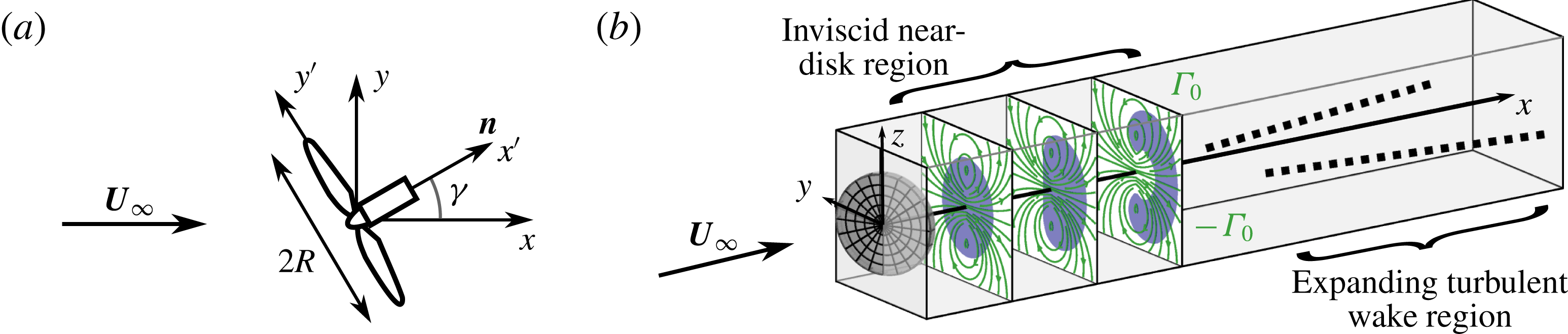
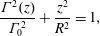
Figure 1. (a) An actuator disk with radius
 $R$
yawed at an angle
$R$
yawed at an angle
 $\unicode[STIX]{x1D6FE}$
. (b) Sketch of the two regions downstream of the rotor: the inviscid region of streamwise velocity deficit, shown in blue, with a counter-rotating vortex pair with circulation
$\unicode[STIX]{x1D6FE}$
. (b) Sketch of the two regions downstream of the rotor: the inviscid region of streamwise velocity deficit, shown in blue, with a counter-rotating vortex pair with circulation
 $\pm \unicode[STIX]{x1D6E4}_{0}$
, superimposed in green, and the expanding turbulent wake region, shown as dashed lines, developing downstream of the inviscid near-disk region.
$\pm \unicode[STIX]{x1D6E4}_{0}$
, superimposed in green, and the expanding turbulent wake region, shown as dashed lines, developing downstream of the inviscid near-disk region.
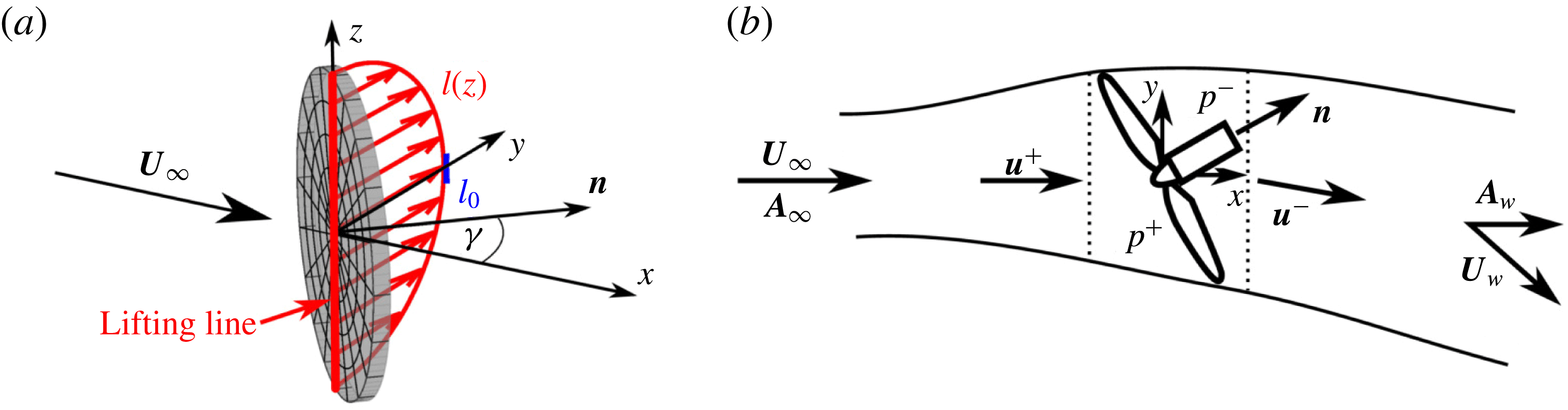
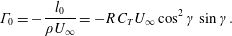
Figure 2. (a) The lifting line segment through the origin between
 $z=-R$
and
$z=-R$
and
 $z=R$
has a lift force per unit span of
$z=R$
has a lift force per unit span of
 $l(z)$
. At
$l(z)$
. At
 $z=0$
the lift is
$z=0$
the lift is
 $l_{0}$
and the circulation is
$l_{0}$
and the circulation is
 $\unicode[STIX]{x1D6E4}_{0}$
. (b) The inviscid streamtube in the near-rotor region of a yawed actuator disk. The rotor region, assumed to be an elliptic cylinder, is between the dotted lines.
$\unicode[STIX]{x1D6E4}_{0}$
. (b) The inviscid streamtube in the near-rotor region of a yawed actuator disk. The rotor region, assumed to be an elliptic cylinder, is between the dotted lines.
As in models of the flow around unyawed actuator disks, we divide the flow into two regions, as shown in figure 1(b). We first consider the predominantly inviscid region near the disk. The description of this region can then be used as an initial condition for models of the wake, where turbulent mixing dominates, as discussed in § 3. In the inviscid region, we first employ the vorticity equation to avoid dealing with pressure fields. In the present context, examining vorticity transport is equivalent to considering the fate of circulation.
The appropriate framework is the Prandtl lifting line theory (Milne-Thomson Reference Milne-Thomson1973), which can be used to predict the transverse velocity, shed circulation, and strength of the counter-rotating vortex pair. To facilitate the use of the Prandtl lifting line theory, we decompose the thrust force into a streamwise force along the
 $x$
-axis and a transverse force along the
$x$
-axis and a transverse force along the
 $y$
-axis, which we refer to as the ‘transverse lift’. The yawed actuator disk can be viewed as an inclined lift-generating surface, akin to an airfoil, with a total span of
$y$
-axis, which we refer to as the ‘transverse lift’. The yawed actuator disk can be viewed as an inclined lift-generating surface, akin to an airfoil, with a total span of
 $2R$
and a chord length
$2R$
and a chord length
 $c(z)$
that varies along the vertical direction
$c(z)$
that varies along the vertical direction
 $z$
. Geometrically, the chord length
$z$
. Geometrically, the chord length
 $c(z)$
is the length of the line segment between the two outer points of the disk at a point
$c(z)$
is the length of the line segment between the two outer points of the disk at a point
 $z$
, expressed mathematically as
$z$
, expressed mathematically as
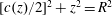 $[c(z)/2]^{2}+z^{2}=R^{2}$
. To apply lifting line theory, the associated lift force can be thought to be distributed along a line segment through the origin between
$[c(z)/2]^{2}+z^{2}=R^{2}$
. To apply lifting line theory, the associated lift force can be thought to be distributed along a line segment through the origin between
 $z=-R$
and
$z=-R$
and
 $z=R$
, as shown in figure 2(a). The lift distribution imposed by the fluid on the actuator disk is assumed to be uniformly distributed over the disk as
$z=R$
, as shown in figure 2(a). The lift distribution imposed by the fluid on the actuator disk is assumed to be uniformly distributed over the disk as
 $$\begin{eqnarray}\displaystyle & \displaystyle L\hspace{0.5pt}{\mathcal{R}}(\boldsymbol{x})\,\boldsymbol{j}=-T\sin \unicode[STIX]{x1D6FE}\,{\mathcal{R}}(\boldsymbol{x})\,\boldsymbol{j}, & \displaystyle\end{eqnarray}$$
where
 $L$
is the total lift force and
$L$
is the total lift force and
 ${\mathcal{R}}(\boldsymbol{x})$
is the area fraction function described above. Therefore, the lift per unit span
${\mathcal{R}}(\boldsymbol{x})$
is the area fraction function described above. Therefore, the lift per unit span
 $l(z)=(L/\unicode[STIX]{x03C0}R^{2})c(z)$
is equal to the lift per unit area times the chord length. Using the geometric relationship
$l(z)=(L/\unicode[STIX]{x03C0}R^{2})c(z)$
is equal to the lift per unit area times the chord length. Using the geometric relationship
 $[c(z)/2]^{2}+z^{2}=R^{2}$
, the resulting distribution of circulation along the span
$[c(z)/2]^{2}+z^{2}=R^{2}$
, the resulting distribution of circulation along the span
 $\unicode[STIX]{x1D6E4}(z)$
, which is related to the lift by
$\unicode[STIX]{x1D6E4}(z)$
, which is related to the lift by
 $l(z)=-\unicode[STIX]{x1D70C}U_{\infty }\unicode[STIX]{x1D6E4}(z)$
, has an elliptic distribution
$l(z)=-\unicode[STIX]{x1D70C}U_{\infty }\unicode[STIX]{x1D6E4}(z)$
, has an elliptic distribution
 $$\begin{eqnarray}\displaystyle & \displaystyle \frac{\unicode[STIX]{x1D6E4}^{2}(z)}{\unicode[STIX]{x1D6E4}_{0}^{2}}+\frac{z^{2}}{R^{2}}=1, & \displaystyle\end{eqnarray}$$
with a maximum circulation magnitude at
 $z=0$
. At
$z=0$
. At
 $z=0$
the chord length is
$z=0$
the chord length is
 $c_{0}=2R$
, the lift is
$c_{0}=2R$
, the lift is
 $l_{0}=2L/(\unicode[STIX]{x03C0}R)=-2T\sin \unicode[STIX]{x1D6FE}/(\unicode[STIX]{x03C0}R)$
, and the circulation is
$l_{0}=2L/(\unicode[STIX]{x03C0}R)=-2T\sin \unicode[STIX]{x1D6FE}/(\unicode[STIX]{x03C0}R)$
, and the circulation is
 $$\begin{eqnarray}\displaystyle & \displaystyle \unicode[STIX]{x1D6E4}_{0}=-\frac{l_{0}}{\unicode[STIX]{x1D70C}U_{\infty }}=-R\,C_{T}U_{\infty }\cos ^{2}\unicode[STIX]{x1D6FE}\sin \unicode[STIX]{x1D6FE}. & \displaystyle\end{eqnarray}$$
According to lifting line theory (Milne-Thomson Reference Milne-Thomson1973), vortex filaments with a strength per unit span
 $\text{d}\unicode[STIX]{x1D6E4}/\text{d}z$
are shed and roll up into counter-rotating trailing vortices at the top and bottom of the disk with strength
$\text{d}\unicode[STIX]{x1D6E4}/\text{d}z$
are shed and roll up into counter-rotating trailing vortices at the top and bottom of the disk with strength
 $$\begin{eqnarray}\displaystyle & \displaystyle \unicode[STIX]{x1D6E4}_{bottom}=-\unicode[STIX]{x1D6E4}_{top}=\int _{-R}^{0}\frac{\text{d}\unicode[STIX]{x1D6E4}}{\text{d}z}\,\text{d}z=\unicode[STIX]{x1D6E4}_{0}. & \displaystyle\end{eqnarray}$$
An elliptic lift distribution is special because it induces a constant transverse velocity (downwash) given by (Milne-Thomson Reference Milne-Thomson1973)
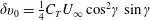
 $$\begin{eqnarray}\displaystyle & \displaystyle \unicode[STIX]{x1D6FF}v_{0}=-\frac{\unicode[STIX]{x1D6E4}_{0}}{4R}=\frac{1}{4}C_{T}U_{\infty }\cos ^{2}\unicode[STIX]{x1D6FE}\sin \unicode[STIX]{x1D6FE}. & \displaystyle\end{eqnarray}$$
Equations (2.5) and (2.7) thus define the transverse behaviour of the inviscid region.

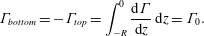
Figure 3. Simulation results for
 $C_{T}^{\prime }=1.33$
and yaw angle
$C_{T}^{\prime }=1.33$
and yaw angle
 $\unicode[STIX]{x1D6FE}=30^{\circ }$
in a domain
$\unicode[STIX]{x1D6FE}=30^{\circ }$
in a domain
 $L_{x}/D=11.52$
and
$L_{x}/D=11.52$
and
 $L_{y}/D=L_{z}/D=5.76$
. Shown are colour contours of (a) streamwise velocity, (b) transverse velocity, and (c) pressure at downstream locations
$L_{y}/D=L_{z}/D=5.76$
. Shown are colour contours of (a) streamwise velocity, (b) transverse velocity, and (c) pressure at downstream locations
 $x/D=1$
, 2, and 3, respectively. Panel (a) includes streamlines in the
$x/D=1$
, 2, and 3, respectively. Panel (a) includes streamlines in the
 $y$
–
$y$
–
 $z$
plane. The transverse velocity and pressure plots show the outline of the wake, defined by the streamtube that passes the rotor at a radius of
$z$
plane. The transverse velocity and pressure plots show the outline of the wake, defined by the streamtube that passes the rotor at a radius of
 $r^{\prime }=0.9R$
.
$r^{\prime }=0.9R$
.
In order to provide data to test predictions based on the proposed model in (2.4)–(2.7), numerical simulations of flow around a yawed actuator disk under uniform, laminar inflow are carried out using the pseudo-spectral code LESGO, which was validated in prior works (e.g. Calaf et al.
Reference Calaf, Meneveau and Meyers2010; Stevens, Martínez & Meneveau Reference Stevens, Martínez and Meneveau2018). A yawed actuator disk of diameter
 $D$
is placed in a domain of length
$D$
is placed in a domain of length
 $L_{x}=11.52D$
and cross-section size
$L_{x}=11.52D$
and cross-section size
 $L_{y}=L_{z}=5.76D$
using a total of
$L_{y}=L_{z}=5.76D$
using a total of
 $384\times 192\times 192$
grid points. The centre of the actuator disk is placed in the centre of a
$384\times 192\times 192$
grid points. The centre of the actuator disk is placed in the centre of a
 $y$
–
$y$
–
 $z$
plane
$z$
plane
 $3.6D$
downstream of the domain inlet. A uniform inflow velocity
$3.6D$
downstream of the domain inlet. A uniform inflow velocity
 $U_{\infty }$
is applied using a fringe region forcing (Stevens, Graham & Meneveau Reference Stevens, Graham and Meneveau2014). Molecular viscosity is neglected and the Smagorinsky model is used for numerical stability with
$U_{\infty }$
is applied using a fringe region forcing (Stevens, Graham & Meneveau Reference Stevens, Graham and Meneveau2014). Molecular viscosity is neglected and the Smagorinsky model is used for numerical stability with
 $C_{s}=0.16$
. Since the flow in the bulk of the near-disk region of interest remains laminar and inviscid and the effect of the subgrid model is confined to the thin shear layer at the boundary of the wake, which is not included in the subsequent analysis, the details of the subgrid modelling are not important for present purposes. The simulations are insensitive to the choice of
$C_{s}=0.16$
. Since the flow in the bulk of the near-disk region of interest remains laminar and inviscid and the effect of the subgrid model is confined to the thin shear layer at the boundary of the wake, which is not included in the subsequent analysis, the details of the subgrid modelling are not important for present purposes. The simulations are insensitive to the choice of
 $C_{s}$
, yielding the same results for
$C_{s}$
, yielding the same results for
 $C_{s}=0.08$
. Various yaw angles
$C_{s}=0.08$
. Various yaw angles
 $\unicode[STIX]{x1D6FE}$
are considered. LESGO uses the local formulation of the thrust force with a local thrust coefficient
$\unicode[STIX]{x1D6FE}$
are considered. LESGO uses the local formulation of the thrust force with a local thrust coefficient
 $C_{T}^{\prime }$
(Calaf et al.
Reference Calaf, Meneveau and Meyers2010). The force is applied using the area fraction function filtered by a three-dimensional Gaussian with a filter width
$C_{T}^{\prime }$
(Calaf et al.
Reference Calaf, Meneveau and Meyers2010). The force is applied using the area fraction function filtered by a three-dimensional Gaussian with a filter width
 $\unicode[STIX]{x1D70E}_{{\mathcal{R}}}=1.5h/\sqrt{12}$
proportional to the grid size
$\unicode[STIX]{x1D70E}_{{\mathcal{R}}}=1.5h/\sqrt{12}$
proportional to the grid size
 $h=(\unicode[STIX]{x0394}x^{2}+\unicode[STIX]{x0394}y^{2}+\unicode[STIX]{x0394}z^{2})^{1/2}$
, where
$h=(\unicode[STIX]{x0394}x^{2}+\unicode[STIX]{x0394}y^{2}+\unicode[STIX]{x0394}z^{2})^{1/2}$
, where
 $\unicode[STIX]{x0394}x$
,
$\unicode[STIX]{x0394}x$
,
 $\unicode[STIX]{x0394}y$
, and
$\unicode[STIX]{x0394}y$
, and
 $\unicode[STIX]{x0394}z$
are the grid spacings.
$\unicode[STIX]{x0394}z$
are the grid spacings.
Representative results at downstream distances
 $x/D=1$
, 2, and 3 are shown in figure 3 for
$x/D=1$
, 2, and 3 are shown in figure 3 for
 $C_{T}^{\prime }=1.33$
and
$C_{T}^{\prime }=1.33$
and
 $\unicode[STIX]{x1D6FE}=30^{\circ }$
. A wake that stays laminar for a large portion of the domain is generated by the actuator disk forcing. At
$\unicode[STIX]{x1D6FE}=30^{\circ }$
. A wake that stays laminar for a large portion of the domain is generated by the actuator disk forcing. At
 $x/D=1$
near the actuator disk, the wake forms an ellipse with uniform streamwise and transverse velocity components inside of the wake. The transverse component of the force generates the well-known counter-rotating vortex pair (Howland et al.
Reference Howland, Bossuyt, Martínez-Tossas, Meyers and Meneveau2016; Bastankhah & Porté-Agel Reference Bastankhah and Porté-Agel2016), which curls the wake as it moves downstream, shown schematically in figure 1(b).
$x/D=1$
near the actuator disk, the wake forms an ellipse with uniform streamwise and transverse velocity components inside of the wake. The transverse component of the force generates the well-known counter-rotating vortex pair (Howland et al.
Reference Howland, Bossuyt, Martínez-Tossas, Meyers and Meneveau2016; Bastankhah & Porté-Agel Reference Bastankhah and Porté-Agel2016), which curls the wake as it moves downstream, shown schematically in figure 1(b).
Further simulations are performed at yaw angles
 $\unicode[STIX]{x1D6FE}=10^{\circ }$
,
$\unicode[STIX]{x1D6FE}=10^{\circ }$
,
 $20^{\circ }$
,
$20^{\circ }$
,
 $30^{\circ }$
, and
$30^{\circ }$
, and
 $40^{\circ }$
and local thrust coefficients
$40^{\circ }$
and local thrust coefficients
 $C_{T}^{\prime }=0.8$
,
$C_{T}^{\prime }=0.8$
,
 $1.0$
, and
$1.0$
, and
 $1.33$
. From these simulations, the spanwise circulation distribution
$1.33$
. From these simulations, the spanwise circulation distribution
 $\unicode[STIX]{x1D6E4}(z)$
is evaluated numerically via integration along rectangular contours running from the inlet of the domain to
$\unicode[STIX]{x1D6E4}(z)$
is evaluated numerically via integration along rectangular contours running from the inlet of the domain to
 $x=R$
and spanning the entire width of the domain. The circulation of each shed vortex
$x=R$
and spanning the entire width of the domain. The circulation of each shed vortex
 $\unicode[STIX]{x1D6E4}_{0}$
is calculated at
$\unicode[STIX]{x1D6E4}_{0}$
is calculated at
 $x=R$
by averaging the circulation around two rectangular circuits spanning
$x=R$
by averaging the circulation around two rectangular circuits spanning
 $|y|\leqslant 3R$
and
$|y|\leqslant 3R$
and
 $|z|\leqslant 3R$
.
$|z|\leqslant 3R$
.
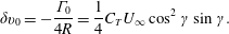
We seek to compare the measured results to (2.4) and (2.5), for which the disk radius is an important parameter. The footprint of the applied force in the simulations extends slightly from the geometrically prescribed disk dimensions, owing to the use of a filtered area fraction function. To correct for the filtered geometric representation of the disk, the width of an equivalent top-hat filter (Pope Reference Pope2000)
 $\sqrt{12}\unicode[STIX]{x1D70E}_{{\mathcal{R}}}=1.5h$
(
$\sqrt{12}\unicode[STIX]{x1D70E}_{{\mathcal{R}}}=1.5h$
(
 $h\ll R$
is the grid size) is added to the diameter of the disk in (2.4) when applying the inviscid model. The resulting effective radius is
$h\ll R$
is the grid size) is added to the diameter of the disk in (2.4) when applying the inviscid model. The resulting effective radius is
 $R_{\ast }=R+0.75h$
, which leads to the predicted maximum circulation being given by
$R_{\ast }=R+0.75h$
, which leads to the predicted maximum circulation being given by
 $\unicode[STIX]{x1D6E4}_{0}=-(R+0.75h)\,C_{T}U_{\infty }\cos ^{2}\unicode[STIX]{x1D6FE}\sin \unicode[STIX]{x1D6FE}$
. The thrust coefficient is obtained from
$\unicode[STIX]{x1D6E4}_{0}=-(R+0.75h)\,C_{T}U_{\infty }\cos ^{2}\unicode[STIX]{x1D6FE}\sin \unicode[STIX]{x1D6FE}$
. The thrust coefficient is obtained from
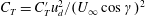
 $C_{T}=C_{T}^{\prime }u_{d}^{2}/(U_{\infty }\cos \unicode[STIX]{x1D6FE})^{2}$
, where the disk-averaged velocity
$C_{T}=C_{T}^{\prime }u_{d}^{2}/(U_{\infty }\cos \unicode[STIX]{x1D6FE})^{2}$
, where the disk-averaged velocity
 $u_{d}$
is measured in the simulations. As seen in the comparison shown in figures 4(a,b), the predicted circulation distribution and simulation results collapse for all
$u_{d}$
is measured in the simulations. As seen in the comparison shown in figures 4(a,b), the predicted circulation distribution and simulation results collapse for all
 $\unicode[STIX]{x1D6FE}$
and
$\unicode[STIX]{x1D6FE}$
and
 $C_{T}^{\prime }$
values tested.
$C_{T}^{\prime }$
values tested.
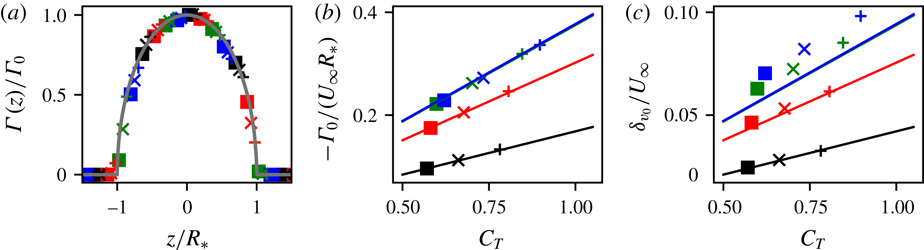
Figure 4. Comparisons of (a) the measured circulation around the actuator disk (symbols) and the expected distribution from the elliptic lifting line
 $(1-z^{2}/R_{\ast }^{2})^{1/2}$
(grey line), (b) the shed circulation of counter-rotating vortices measured at
$(1-z^{2}/R_{\ast }^{2})^{1/2}$
(grey line), (b) the shed circulation of counter-rotating vortices measured at
 $x=R$
(symbols) and predicted by lifting line theory (lines), and (c) the maximum
$x=R$
(symbols) and predicted by lifting line theory (lines), and (c) the maximum
 $y$
–
$y$
–
 $z$
planar-averaged transverse velocity measured in the streamtube (symbols) and transverse velocity predicted by lifting line theory (lines). Simulations are conducted with
$z$
planar-averaged transverse velocity measured in the streamtube (symbols) and transverse velocity predicted by lifting line theory (lines). Simulations are conducted with
 $\unicode[STIX]{x1D6FE}=10^{\circ }$
(black),
$\unicode[STIX]{x1D6FE}=10^{\circ }$
(black),
 $20^{\circ }$
(red),
$20^{\circ }$
(red),
 $30^{\circ }$
(green), and
$30^{\circ }$
(green), and
 $40^{\circ }$
(blue) and
$40^{\circ }$
(blue) and
 $C_{T}^{\prime }=0.8$
(▪), 1.0 (
$C_{T}^{\prime }=0.8$
(▪), 1.0 (
 $\times$
), and 1.33 (
$\times$
), and 1.33 (
 $+$
). The theoretical values for
$+$
). The theoretical values for
 $\unicode[STIX]{x1D6FE}=30^{\circ }$
and
$\unicode[STIX]{x1D6FE}=30^{\circ }$
and
 $40^{\circ }$
overlap in (b) and (c).
$40^{\circ }$
overlap in (b) and (c).
Next we compare the transverse velocity magnitude
 $\unicode[STIX]{x1D6FF}v_{0}$
with the model. To measure this value from simulations we take the maximum
$\unicode[STIX]{x1D6FF}v_{0}$
with the model. To measure this value from simulations we take the maximum
 $y$
–
$y$
–
 $z$
planar-averaged transverse velocity in the wake. The wake is defined as the streamtube passing through the disk at
$z$
planar-averaged transverse velocity in the wake. The wake is defined as the streamtube passing through the disk at
 $r^{\prime }=0.9R$
to avoid including the thin shear layer near the actuator disk perimeter (results are quite insensitive to this choice). The downstream position of maximum transverse wake velocity occurs very near the disk, at
$r^{\prime }=0.9R$
to avoid including the thin shear layer near the actuator disk perimeter (results are quite insensitive to this choice). The downstream position of maximum transverse wake velocity occurs very near the disk, at
 $x\approx R$
. Using the thrust coefficient obtained from
$x\approx R$
. Using the thrust coefficient obtained from
 $C_{T}=C_{T}^{\prime }u_{d}^{2}/(U_{\infty }\cos \unicode[STIX]{x1D6FE})^{2}$
, we compare
$C_{T}=C_{T}^{\prime }u_{d}^{2}/(U_{\infty }\cos \unicode[STIX]{x1D6FE})^{2}$
, we compare
 $\unicode[STIX]{x1D6FF}v_{0}=\frac{1}{4}C_{T}U_{\infty }\,\text{cos}^{2}\unicode[STIX]{x1D6FE}\,\text{sin}\,\unicode[STIX]{x1D6FE}$
to simulation measurements in figure 4(c). Again, excellent agreement is observed for various
$\unicode[STIX]{x1D6FF}v_{0}=\frac{1}{4}C_{T}U_{\infty }\,\text{cos}^{2}\unicode[STIX]{x1D6FE}\,\text{sin}\,\unicode[STIX]{x1D6FE}$
to simulation measurements in figure 4(c). Again, excellent agreement is observed for various
 $\unicode[STIX]{x1D6FE}$
and
$\unicode[STIX]{x1D6FE}$
and
 $C_{T}^{\prime }$
combinations, with a slight underestimate at large
$C_{T}^{\prime }$
combinations, with a slight underestimate at large
 $\unicode[STIX]{x1D6FE}$
.
$\unicode[STIX]{x1D6FE}$
.
In addition to the transverse velocity derived, additional expressions are needed to fully describe the inviscid region near the yawed actuator disk. The induced velocity through the disk, as well as the streamwise velocity deficit in the wake, are derived using an approach similar to the unyawed momentum theory (Glauert Reference Glauert1935; Burton et al.
Reference Burton, Jenkins, Sharpe and Bossanyi2011). The streamtube through the rotor is used as a control volume and the velocity is assumed to be uniform across every cross-section, as shown in figure 2(b). The velocities upstream of the rotor and at the end of the inviscid region (beginning of the wake) are denoted by
 $\boldsymbol{U}_{\infty }$
and
$\boldsymbol{U}_{\infty }$
and
 $\boldsymbol{U}_{w}$
, respectively. Also, at those locations we consider flow through vertical sections with area vectors,
$\boldsymbol{U}_{w}$
, respectively. Also, at those locations we consider flow through vertical sections with area vectors,
 $\boldsymbol{A}_{\infty }=A_{\infty }\,\boldsymbol{i}$
and
$\boldsymbol{A}_{\infty }=A_{\infty }\,\boldsymbol{i}$
and
 $\boldsymbol{A}_{w}=A_{w}\,\boldsymbol{i}$
, defined in figure 2(b). The disk-averaged velocity
$\boldsymbol{A}_{w}=A_{w}\,\boldsymbol{i}$
, defined in figure 2(b). The disk-averaged velocity
 $u_{d}$
through the disk area
$u_{d}$
through the disk area
 $A_{d}=\unicode[STIX]{x03C0}R^{2}$
and mass conservation yields
$A_{d}=\unicode[STIX]{x03C0}R^{2}$
and mass conservation yields
 $u_{d}A_{d}=\boldsymbol{U}_{\infty }\boldsymbol{\cdot }\boldsymbol{A}_{\infty }=\boldsymbol{U}_{w}\boldsymbol{\cdot }\boldsymbol{A}_{w}$
, where the dots indicate inner products. The wake velocity is written as
$u_{d}A_{d}=\boldsymbol{U}_{\infty }\boldsymbol{\cdot }\boldsymbol{A}_{\infty }=\boldsymbol{U}_{w}\boldsymbol{\cdot }\boldsymbol{A}_{w}$
, where the dots indicate inner products. The wake velocity is written as
 $\boldsymbol{U}_{w}=(U_{\infty }-\unicode[STIX]{x1D6FF}u_{0})\boldsymbol{i}-\unicode[STIX]{x1D6FF}v_{0}\,\boldsymbol{j}$
, where
$\boldsymbol{U}_{w}=(U_{\infty }-\unicode[STIX]{x1D6FF}u_{0})\boldsymbol{i}-\unicode[STIX]{x1D6FF}v_{0}\,\boldsymbol{j}$
, where
 $\unicode[STIX]{x1D6FF}u_{0}$
is the streamwise velocity deficit and
$\unicode[STIX]{x1D6FF}u_{0}$
is the streamwise velocity deficit and
 $\unicode[STIX]{x1D6FF}v_{0}$
is the transverse velocity magnitude specified by the lifting line theory in (2.7).
$\unicode[STIX]{x1D6FF}v_{0}$
is the transverse velocity magnitude specified by the lifting line theory in (2.7).
The region of the streamtube cut by the actuator disk is treated as an elliptic cylinder with a cross-sectional area of
 $A_{d}\cos \unicode[STIX]{x1D6FE}$
. Inside this volume, the upstream and downstream pressure are assumed to be constant at
$A_{d}\cos \unicode[STIX]{x1D6FE}$
. Inside this volume, the upstream and downstream pressure are assumed to be constant at
 $p^{+}$
and
$p^{+}$
and
 $p^{-}$
, respectively. The upstream and downstream velocities are respectively
$p^{-}$
, respectively. The upstream and downstream velocities are respectively
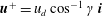 $\boldsymbol{u}^{+}=u_{d}\cos ^{-1}\unicode[STIX]{x1D6FE}\,\boldsymbol{i}$
and
$\boldsymbol{u}^{+}=u_{d}\cos ^{-1}\unicode[STIX]{x1D6FE}\,\boldsymbol{i}$
and
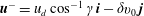 $\boldsymbol{u}^{-}=u_{d}\cos ^{-1}\unicode[STIX]{x1D6FE}\boldsymbol{i}-\unicode[STIX]{x1D6FF}v_{0}\,\boldsymbol{j}$
. The streamwise velocity through this region is assumed to be constant and is determined using mass conservation. The transverse velocity has a discontinuity at the disk, jumping from zero to the downwash
$\boldsymbol{u}^{-}=u_{d}\cos ^{-1}\unicode[STIX]{x1D6FE}\boldsymbol{i}-\unicode[STIX]{x1D6FF}v_{0}\,\boldsymbol{j}$
. The streamwise velocity through this region is assumed to be constant and is determined using mass conservation. The transverse velocity has a discontinuity at the disk, jumping from zero to the downwash
 $-\unicode[STIX]{x1D6FF}v_{0}$
behind the rotor region.
$-\unicode[STIX]{x1D6FF}v_{0}$
behind the rotor region.
Assuming that the streamwise pressure force vanishes over the streamtube’s surface, as in the unyawed case (Glauert Reference Glauert1935), the streamwise momentum equation is
 $$\begin{eqnarray}\displaystyle & \displaystyle -\unicode[STIX]{x1D70C}\,\boldsymbol{U}_{\infty }\boldsymbol{\cdot }\boldsymbol{A}_{\infty }\,U_{\infty }+\unicode[STIX]{x1D70C}\,\boldsymbol{U}_{w}\boldsymbol{\cdot }\boldsymbol{A}_{w}\,(U_{\infty }-\unicode[STIX]{x1D6FF}u_{0})=T\cos \unicode[STIX]{x1D6FE}. & \displaystyle\end{eqnarray}$$
The Bernoulli equation is then applied from far upstream to where
 $p=p^{+}$
and from where
$p=p^{+}$
and from where
 $p=p^{-}$
to further downstream of the turbine where
$p=p^{-}$
to further downstream of the turbine where
 $p$
recovers and the turbulent wake begins, as shown in figure 2(b). Assuming that
$p$
recovers and the turbulent wake begins, as shown in figure 2(b). Assuming that
 $\unicode[STIX]{x1D6FF}v_{0}$
remains constant in the downstream part of the inviscid region, we write
$\unicode[STIX]{x1D6FF}v_{0}$
remains constant in the downstream part of the inviscid region, we write
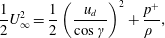 $$\begin{eqnarray}\displaystyle & \displaystyle \frac{1}{2}U_{\infty }^{2}=\frac{1}{2}\left(\frac{u_{d}}{\cos \unicode[STIX]{x1D6FE}}\right)^{2}+\frac{p^{+}}{\unicode[STIX]{x1D70C}~}, & \displaystyle\end{eqnarray}$$
 $$\begin{eqnarray}\displaystyle & \displaystyle \frac{1}{2}\left(\frac{u_{d}}{\cos \unicode[STIX]{x1D6FE}}\right)^{2}+\frac{1}{2}\unicode[STIX]{x1D6FF}v_{0}^{2}+\frac{p^{-}}{\unicode[STIX]{x1D70C}~}=\frac{1}{2}(U_{\infty }-\unicode[STIX]{x1D6FF}u_{0})^{2}+\frac{1}{2}\unicode[STIX]{x1D6FF}v_{0}^{2}. & \displaystyle\end{eqnarray}$$
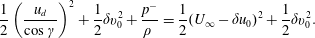
 $(p^{+}-p^{-})A_{d}=-T$
, we obtain
$(p^{+}-p^{-})A_{d}=-T$
, we obtain 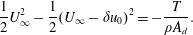 $$\begin{eqnarray}\displaystyle & \displaystyle \frac{1}{2}U_{\infty }^{2}-\frac{1}{2}(U_{\infty }-\unicode[STIX]{x1D6FF}u_{0})^{2}=-\frac{T}{\unicode[STIX]{x1D70C}A_{d}}. & \displaystyle\end{eqnarray}$$
Substituting the thrust force (2.2) and mass flow rate into (2.8) and (2.10) yields two equations for the unknown disk-averaged velocity and streamwise velocity deficit
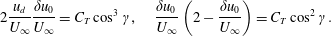 $$\begin{eqnarray}\displaystyle & \displaystyle 2\frac{u_{d}}{U_{\infty }}\frac{\unicode[STIX]{x1D6FF}u_{0}}{U_{\infty }}=C_{T}\cos ^{3}\unicode[STIX]{x1D6FE},\quad \frac{\unicode[STIX]{x1D6FF}u_{0}}{U_{\infty }}\left(2-\frac{\unicode[STIX]{x1D6FF}u_{0}}{U_{\infty }}\right)=C_{T}\cos ^{2}\unicode[STIX]{x1D6FE}. & \displaystyle\end{eqnarray}$$
Written in terms of the induction factor
 $a$
, the solution is
$a$
, the solution is
 $$\begin{eqnarray}\displaystyle & \displaystyle u_{d}/U_{\infty }=\cos \unicode[STIX]{x1D6FE}(1-a),\quad \unicode[STIX]{x1D6FF}u_{0}/U_{\infty }=2a, & \displaystyle\end{eqnarray}$$
where the thrust coefficient is related to the induction factor by
 $C_{T}\cos ^{2}\unicode[STIX]{x1D6FE}=4a(1-a)$
. The induction factor can subsequently be written in terms of both the standard and local thrust coefficients using the identity
$C_{T}\cos ^{2}\unicode[STIX]{x1D6FE}=4a(1-a)$
. The induction factor can subsequently be written in terms of both the standard and local thrust coefficients using the identity
 $C_{T}U_{\infty }^{2}\cos ^{2}\unicode[STIX]{x1D6FE}=C_{T}^{\prime }u_{d}^{2}$
according to
$C_{T}U_{\infty }^{2}\cos ^{2}\unicode[STIX]{x1D6FE}=C_{T}^{\prime }u_{d}^{2}$
according to
 $$\begin{eqnarray}\displaystyle & \displaystyle a=\frac{C_{T}^{\prime }\cos ^{2}\unicode[STIX]{x1D6FE}}{4+C_{T}^{\prime }\cos ^{2}\unicode[STIX]{x1D6FE}}=\frac{1}{2}\left(1-\sqrt{1-C_{T}\cos ^{2}\unicode[STIX]{x1D6FE}}\right). & \displaystyle\end{eqnarray}$$
The initial skewness angle is obtained from
 $\tan \unicode[STIX]{x1D6FC}=-\unicode[STIX]{x1D6FF}v_{0}/(U_{\infty }-\unicode[STIX]{x1D6FF}u_{0})$
.
$\tan \unicode[STIX]{x1D6FC}=-\unicode[STIX]{x1D6FF}v_{0}/(U_{\infty }-\unicode[STIX]{x1D6FF}u_{0})$
.

Figure 5. Comparison of (a) transverse velocity
 $\unicode[STIX]{x1D6FF}v_{0}/U_{\infty }$
, (b) disk-averaged velocity
$\unicode[STIX]{x1D6FF}v_{0}/U_{\infty }$
, (b) disk-averaged velocity
 $u_{d}/U_{\infty }$
, (c) streamwise velocity
$u_{d}/U_{\infty }$
, (c) streamwise velocity
 $1-\unicode[STIX]{x1D6FF}u_{0}/U_{\infty }$
, and (d) skewness angle
$1-\unicode[STIX]{x1D6FF}u_{0}/U_{\infty }$
, and (d) skewness angle
 $\unicode[STIX]{x1D6FC}$
measured in simulations with
$\unicode[STIX]{x1D6FC}$
measured in simulations with
 $C_{T}^{\prime }=1.0$
(squares) with present theory (solid black line) and prior models (other lines).
$C_{T}^{\prime }=1.0$
(squares) with present theory (solid black line) and prior models (other lines).
The disk-averaged velocity, streamwise velocity deficit, transverse velocity, and skewness angle of the initial wake obtained from numerical simulations, the present model, and prior models are compared in figure 5. The velocity deficit
 $\unicode[STIX]{x1D6FF}u_{0}$
at the end of the inviscid region is obtained from the simulations as the maximum
$\unicode[STIX]{x1D6FF}u_{0}$
at the end of the inviscid region is obtained from the simulations as the maximum
 $y$
–
$y$
–
 $z$
planar-averaged streamwise velocity deficit in the wake, which occurs at
$z$
planar-averaged streamwise velocity deficit in the wake, which occurs at
 $x\approx 4D$
. The maximum for
$x\approx 4D$
. The maximum for
 $\unicode[STIX]{x1D6FF}u_{0}$
is further downstream than the maximum for
$\unicode[STIX]{x1D6FF}u_{0}$
is further downstream than the maximum for
 $\unicode[STIX]{x1D6FF}v_{0}$
because
$\unicode[STIX]{x1D6FF}v_{0}$
because
 $\unicode[STIX]{x1D6FF}u_{0}$
is strongly affected by streamwise pressure gradients. The transverse velocity prediction (2.7) is expressed using the thrust coefficient
$\unicode[STIX]{x1D6FF}u_{0}$
is strongly affected by streamwise pressure gradients. The transverse velocity prediction (2.7) is expressed using the thrust coefficient
 $C_{T}=16C_{T}^{\prime }/(4+C_{T}^{\prime }\cos ^{2}\unicode[STIX]{x1D6FE})^{2}$
obtained from the induction factor (2.13). Predictions for several of the features of the inviscid region are provided by earlier models. Momentum theory (Burton et al.
Reference Burton, Jenkins, Sharpe and Bossanyi2011) provides estimates for all quantities. Glauert’s (Reference Glauert1926) equation for the disk-averaged velocity was used by Coleman et al. (Reference Coleman, Feingold and Stempin1945; Burton et al.
Reference Burton, Jenkins, Sharpe and Bossanyi2011) to predict the skewness angle of the wake. Bastankhah & Porté-Agel (Reference Bastankhah and Porté-Agel2016) recently used momentum conservation, the Bernoulli equation, and approximations to Glauert’s and Coleman’s equations to predict the streamwise and transverse velocities behind the disk. Jiménez et al. (Reference Jiménez, Crespo and Migoya2010) used momentum balance arguments to predict the initial wake deflection angle.
$C_{T}=16C_{T}^{\prime }/(4+C_{T}^{\prime }\cos ^{2}\unicode[STIX]{x1D6FE})^{2}$
obtained from the induction factor (2.13). Predictions for several of the features of the inviscid region are provided by earlier models. Momentum theory (Burton et al.
Reference Burton, Jenkins, Sharpe and Bossanyi2011) provides estimates for all quantities. Glauert’s (Reference Glauert1926) equation for the disk-averaged velocity was used by Coleman et al. (Reference Coleman, Feingold and Stempin1945; Burton et al.
Reference Burton, Jenkins, Sharpe and Bossanyi2011) to predict the skewness angle of the wake. Bastankhah & Porté-Agel (Reference Bastankhah and Porté-Agel2016) recently used momentum conservation, the Bernoulli equation, and approximations to Glauert’s and Coleman’s equations to predict the streamwise and transverse velocities behind the disk. Jiménez et al. (Reference Jiménez, Crespo and Migoya2010) used momentum balance arguments to predict the initial wake deflection angle.
Figure 5 shows that the present inviscid region model accurately predicts the quantities measured in simulations. In contrast, the other models show significant disagreement in the skewness angle and transverse velocities. Momentum theory and Jiménez’s equation overestimate the skewness angle and transverse velocity magnitudes. The skewness angle magnitude predicted by Coleman et al. (Reference Coleman, Feingold and Stempin1945), and by extension the transverse velocity magnitude predicted by Bastankhah & Porté-Agel (Reference Bastankhah and Porté-Agel2016), are approximately half as large as those obtained in the simulations. While Coleman’s (Reference Coleman, Feingold and Stempin1945) prediction may improve downstream as the wake is transformed by the counter-rotating vortex pair, this skewed elliptic vortex cylinder argument becomes less valid as a result of the curling.
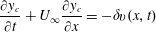
3 Wake model for yawed turbines
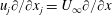
An important application of the inviscid region theory described in the prior section is to determine an initial condition for models of the turbulent wake behind yawed turbines. We demonstrate the utility of the proposed inviscid region model by applying the predictions to the wake model of Shapiro et al. (Reference Shapiro, Bauweraerts, Meyers, Meneveau and Gayme2017), which we extend below to include yaw. As in Shapiro et al. (Reference Shapiro, Bauweraerts, Meyers, Meneveau and Gayme2017), the derivation includes possible time dependence (e.g. the turbine’s local thrust coefficient and yaw angle could change over time). In this paper, however, we focus solely on the steady-state solution and compare it to the wind tunnel experiments of Bastankhah & Porté-Agel (Reference Bastankhah and Porté-Agel2016) that were performed under steady conditions. After neglecting the viscous terms, linearizing the advective term, i.e.
 $u_{j}\unicode[STIX]{x2202}/\unicode[STIX]{x2202}x_{j}=U_{\infty }\unicode[STIX]{x2202}/\unicode[STIX]{x2202}x$
, and rewriting in terms of the mean velocity deficit
$u_{j}\unicode[STIX]{x2202}/\unicode[STIX]{x2202}x_{j}=U_{\infty }\unicode[STIX]{x2202}/\unicode[STIX]{x2202}x$
, and rewriting in terms of the mean velocity deficit
 $U_{\infty }\unicode[STIX]{x1D6FF}_{i1}-u_{i}(\boldsymbol{x},t)$
, the Reynolds averaged mean momentum equation becomes
$U_{\infty }\unicode[STIX]{x1D6FF}_{i1}-u_{i}(\boldsymbol{x},t)$
, the Reynolds averaged mean momentum equation becomes
 $$\begin{eqnarray}\displaystyle & \displaystyle \unicode[STIX]{x1D70C}\frac{\unicode[STIX]{x2202}}{\unicode[STIX]{x2202}t}(U_{\infty }\unicode[STIX]{x1D6FF}_{i1}-u_{i})+\unicode[STIX]{x1D70C}U_{\infty }\frac{\unicode[STIX]{x2202}}{\unicode[STIX]{x2202}x}(U_{\infty }\unicode[STIX]{x1D6FF}_{i1}-u_{i})=\frac{\unicode[STIX]{x2202}p}{\unicode[STIX]{x2202}x_{i}}-f_{i}+\frac{\unicode[STIX]{x2202}\unicode[STIX]{x1D70F}_{ij}}{\unicode[STIX]{x2202}x_{j}}, & \displaystyle\end{eqnarray}$$
where
 $p(\boldsymbol{x},t)$
is the pressure,
$p(\boldsymbol{x},t)$
is the pressure,
 $f_{i}(\boldsymbol{x},t)$
is the turbine thrust force, and
$f_{i}(\boldsymbol{x},t)$
is the turbine thrust force, and
 $\unicode[STIX]{x1D70F}_{ij}$
the Reynolds stress tensor. The area of the wake downstream of the turbine expands due to turbulent mixing. If the expansion rate is determined only by the turbulence properties of the incoming flow, then the effective area of the wake
$\unicode[STIX]{x1D70F}_{ij}$
the Reynolds stress tensor. The area of the wake downstream of the turbine expands due to turbulent mixing. If the expansion rate is determined only by the turbulence properties of the incoming flow, then the effective area of the wake
 $A(x)$
can be assumed to be a function of only the streamwise distance
$A(x)$
can be assumed to be a function of only the streamwise distance
 $x$
from the turbine. Assuming that this effective area is known, the mean velocity deficit
$x$
from the turbine. Assuming that this effective area is known, the mean velocity deficit
 $\unicode[STIX]{x1D6FF}\boldsymbol{u}(x,t)=\unicode[STIX]{x1D6FF}u\,\boldsymbol{i}+\unicode[STIX]{x1D6FF}v\,\boldsymbol{j}$
is defined as
$\unicode[STIX]{x1D6FF}\boldsymbol{u}(x,t)=\unicode[STIX]{x1D6FF}u\,\boldsymbol{i}+\unicode[STIX]{x1D6FF}v\,\boldsymbol{j}$
is defined as
 $$\begin{eqnarray}\displaystyle & \displaystyle \unicode[STIX]{x1D6FF}u_{i}(x,t)=\frac{1}{A(x)}\int _{-\infty }^{\infty }\int _{-\infty }^{\infty }(U_{\infty }\unicode[STIX]{x1D6FF}_{i1}-u_{i}(x,y,z,t))\,\text{d}y\,\text{d}z. & \displaystyle\end{eqnarray}$$
Integrating (3.1) in the transverse directions yields
 $$\begin{eqnarray}\displaystyle & \displaystyle \frac{\unicode[STIX]{x2202}}{\unicode[STIX]{x2202}t}\left[\unicode[STIX]{x1D70C}A(x)\unicode[STIX]{x1D6FF}u_{i}(x,t)\right]+U_{\infty }\frac{\unicode[STIX]{x2202}}{\unicode[STIX]{x2202}x}\left[\unicode[STIX]{x1D70C}A(x)\unicode[STIX]{x1D6FF}u_{i}(x,t)\right]=\frac{\unicode[STIX]{x2202}\bar{p}}{\unicode[STIX]{x2202}x}\unicode[STIX]{x1D6FF}_{i1}-\bar{f}_{i}, & \displaystyle\end{eqnarray}$$
where
 $\bar{p}(x,t)$
and
$\bar{p}(x,t)$
and
 $\bar{f}_{i}(x,t)$
are the transversely averaged pressure and thrust force. Although the divergence of the Reynolds stress does not enter, the effects of turbulence are encoded in the modelled behaviour of
$\bar{f}_{i}(x,t)$
are the transversely averaged pressure and thrust force. Although the divergence of the Reynolds stress does not enter, the effects of turbulence are encoded in the modelled behaviour of
 $A(x)$
.
$A(x)$
.
Since the thrust force is confined to the rotor disk and the pressure gradient vanishes away from the turbine (Glauert Reference Glauert1935), the right-hand side of (3.3) only has to be considered in the region near the turbine rotor. The net effect of the pressure gradient and thrust force is therefore modelled as a source of momentum deficit
 $\unicode[STIX]{x2202}\bar{p}/\unicode[STIX]{x2202}x\,\unicode[STIX]{x1D6FF}_{i1}-\bar{f}_{i}=\unicode[STIX]{x1D70C}A(x)\,S_{i}\,\unicode[STIX]{x1D6FF}(x),$
where
$\unicode[STIX]{x2202}\bar{p}/\unicode[STIX]{x2202}x\,\unicode[STIX]{x1D6FF}_{i1}-\bar{f}_{i}=\unicode[STIX]{x1D70C}A(x)\,S_{i}\,\unicode[STIX]{x1D6FF}(x),$
where
 $S_{i}$
may be time dependent in cases of varying turbine thrust. Substituting into (3.3), expanding the spatial derivatives, and dividing by
$S_{i}$
may be time dependent in cases of varying turbine thrust. Substituting into (3.3), expanding the spatial derivatives, and dividing by
 $\unicode[STIX]{x1D70C}A(x)$
yields
$\unicode[STIX]{x1D70C}A(x)$
yields
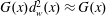
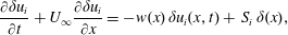 $$\begin{eqnarray}\displaystyle & \displaystyle \frac{\unicode[STIX]{x2202}\unicode[STIX]{x1D6FF}u_{i}}{\unicode[STIX]{x2202}t}+U_{\infty }\frac{\unicode[STIX]{x2202}\unicode[STIX]{x1D6FF}u_{i}}{\unicode[STIX]{x2202}x}=-w(x)\,\unicode[STIX]{x1D6FF}u_{i}(x,t)+\,S_{i}\,\unicode[STIX]{x1D6FF}(x), & \displaystyle\end{eqnarray}$$
where
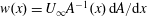 $w(x)=U_{\infty }A^{-1}(x)\,\text{d}A/\text{d}x$
is the wake expansion rate. To model the velocity deficit field in a smooth manner, the Dirac delta function in (3.4) is replaced by a normalized Gaussian function
$w(x)=U_{\infty }A^{-1}(x)\,\text{d}A/\text{d}x$
is the wake expansion rate. To model the velocity deficit field in a smooth manner, the Dirac delta function in (3.4) is replaced by a normalized Gaussian function
 $G(x)$
with characteristic width
$G(x)$
with characteristic width
 $\unicode[STIX]{x0394}_{w}=R$
. Furthermore, the wake area is written as
$\unicode[STIX]{x0394}_{w}=R$
. Furthermore, the wake area is written as
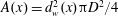 $A(x)=d_{w}^{2}(x)\unicode[STIX]{x03C0}D^{2}/4$
, where
$A(x)=d_{w}^{2}(x)\unicode[STIX]{x03C0}D^{2}/4$
, where
 $d_{w}(x)$
is the effective diameter of the wake normalized by turbine diameter
$d_{w}(x)$
is the effective diameter of the wake normalized by turbine diameter
 $D$
defined by
$D$
defined by
 $d_{w}(x)=1+k_{w}\ln (1+\exp [(x-2\unicode[STIX]{x0394}_{w})/R])$
. This effective diameter
$d_{w}(x)=1+k_{w}\ln (1+\exp [(x-2\unicode[STIX]{x0394}_{w})/R])$
. This effective diameter
 $d_{w}(x)$
tends towards the Jensen (Reference Jensen1983) model’s linear expansion in the wake with expansion coefficient
$d_{w}(x)$
tends towards the Jensen (Reference Jensen1983) model’s linear expansion in the wake with expansion coefficient
 $k_{w}$
, but stays above 1 and begins to expand only at
$k_{w}$
, but stays above 1 and begins to expand only at
 $x\sim 2\unicode[STIX]{x0394}_{w}$
to prevent wake expansion within the zone of the Gaussian forcing. The velocity deficit source strengths,
$x\sim 2\unicode[STIX]{x0394}_{w}$
to prevent wake expansion within the zone of the Gaussian forcing. The velocity deficit source strengths,
 $S_{1}=U_{\infty }\unicode[STIX]{x1D6FF}u_{0}$
and
$S_{1}=U_{\infty }\unicode[STIX]{x1D6FF}u_{0}$
and
 $S_{2}=U_{\infty }\unicode[STIX]{x1D6FF}v_{0}$
, are based on the inviscid model, where
$S_{2}=U_{\infty }\unicode[STIX]{x1D6FF}v_{0}$
, are based on the inviscid model, where
 $\unicode[STIX]{x1D6FF}u_{0}$
and
$\unicode[STIX]{x1D6FF}u_{0}$
and
 $\unicode[STIX]{x1D6FF}v_{0}$
are given by (2.12) and (2.7). This approach provides a smooth increase of the streamwise and transverse velocity deficits from zero upstream of the rotor to the desired ‘wake initial condition’ downstream of the rotor region.
$\unicode[STIX]{x1D6FF}v_{0}$
are given by (2.12) and (2.7). This approach provides a smooth increase of the streamwise and transverse velocity deficits from zero upstream of the rotor to the desired ‘wake initial condition’ downstream of the rotor region.

Figure 6. Hub-height colour contour plots of streamwise velocity as (a) measured in experiments (Bastankhah & Porté-Agel Reference Bastankhah and Porté-Agel2016) and (b) predicted using the proposed model. Measured centrelines of the wake (dotted) are compared to the model of Jiménez et al. (Reference Jiménez, Crespo and Migoya2010) (solid) and the present model (dashed). Experimental data in (a) adapted with permission from figure 3 of Bastankhah & Porté-Agel (Reference Bastankhah and Porté-Agel2016).
The average streamwise velocity deficit
 $\unicode[STIX]{x1D6FF}u(x,t)$
is distributed using a Gaussian profile (Bastankhah & Porté-Agel Reference Bastankhah and Porté-Agel2014, Reference Bastankhah and Porté-Agel2016), which along
$\unicode[STIX]{x1D6FF}u(x,t)$
is distributed using a Gaussian profile (Bastankhah & Porté-Agel Reference Bastankhah and Porté-Agel2014, Reference Bastankhah and Porté-Agel2016), which along
 $z=0$
reads
$z=0$
reads
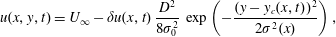 $$\begin{eqnarray}\displaystyle & \displaystyle u(x,y,t)=U_{\infty }-\unicode[STIX]{x1D6FF}u(x,t)\,\frac{D^{2}}{8\unicode[STIX]{x1D70E}_{0}^{2}}\,\exp \left(-\frac{(y-y_{c}(x,t))^{2}}{2\unicode[STIX]{x1D70E}^{2}(x)}\right), & \displaystyle\end{eqnarray}$$
where the width of the Gaussian
 $\unicode[STIX]{x1D70E}(x)=\unicode[STIX]{x1D70E}_{0}d_{w}(x)$
is proportional to the effective normalized wake diameter with a proportionality constant
$\unicode[STIX]{x1D70E}(x)=\unicode[STIX]{x1D70E}_{0}d_{w}(x)$
is proportional to the effective normalized wake diameter with a proportionality constant
 $\unicode[STIX]{x1D70E}_{0}$
. The velocity deficits are found by integrating (3.4), and the wake centreline
$\unicode[STIX]{x1D70E}_{0}$
. The velocity deficits are found by integrating (3.4), and the wake centreline
 $y_{c}(x,t)$
is found by integrating the transverse velocity according to
$y_{c}(x,t)$
is found by integrating the transverse velocity according to
 $$\begin{eqnarray}\displaystyle & \displaystyle \frac{\unicode[STIX]{x2202}y_{c}}{\unicode[STIX]{x2202}t}+U_{\infty }\frac{\unicode[STIX]{x2202}y_{c}}{\unicode[STIX]{x2202}x}=-\unicode[STIX]{x1D6FF}v(x,t) & \displaystyle\end{eqnarray}$$
in the positive
 $x$
direction subject to
$x$
direction subject to
 $y_{c}=0$
far upstream of the turbine. The negative sign occurs because
$y_{c}=0$
far upstream of the turbine. The negative sign occurs because
 $\unicode[STIX]{x1D6FF}v(x,t)$
is a deficit in our sign convention. Equation (3.5) is consistent with (3.2); i.e.
$\unicode[STIX]{x1D6FF}v(x,t)$
is a deficit in our sign convention. Equation (3.5) is consistent with (3.2); i.e.
 $\int _{0}^{\infty }(U_{\infty }-u)2\unicode[STIX]{x03C0}\unicode[STIX]{x1D709}\,\text{d}\unicode[STIX]{x1D709}=A(x)\unicode[STIX]{x1D6FF}u(x,t)$
, where the distance
$\int _{0}^{\infty }(U_{\infty }-u)2\unicode[STIX]{x03C0}\unicode[STIX]{x1D709}\,\text{d}\unicode[STIX]{x1D709}=A(x)\unicode[STIX]{x1D6FF}u(x,t)$
, where the distance
 $\unicode[STIX]{x1D709}=y-y_{c}(x,t)$
is measured from the wake centreline at
$\unicode[STIX]{x1D709}=y-y_{c}(x,t)$
is measured from the wake centreline at
 $y_{c}(x,t)$
.
$y_{c}(x,t)$
.
The steady-state version of this wake model, where time derivatives vanish and the solution found by integrating in
 $x$
and noting
$x$
and noting
 $G(x)d_{w}^{2}(x)\approx G(x)$
,
$G(x)d_{w}^{2}(x)\approx G(x)$
,
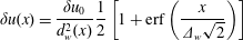 $$\begin{eqnarray}\displaystyle & \displaystyle \unicode[STIX]{x1D6FF}u(x)=\frac{\unicode[STIX]{x1D6FF}u_{0}}{d_{w}^{2}(x)}\frac{1}{2}\left[1+\text{erf}\left(\frac{x}{\unicode[STIX]{x1D6E5}_{w}\sqrt{2}}\right)\right] & \displaystyle\end{eqnarray}$$
 $$\begin{eqnarray}\displaystyle & \displaystyle \unicode[STIX]{x1D6FF}v(x)=\frac{\unicode[STIX]{x1D6FF}v_{0}}{d_{w}^{2}(x)}\frac{1}{2}\left[1+\text{erf}\left(\frac{x}{\unicode[STIX]{x1D6E5}_{w}\sqrt{2}}\right)\right] & \displaystyle\end{eqnarray}$$
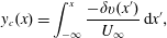 $$\begin{eqnarray}\displaystyle & \displaystyle y_{c}(x)=\int _{-\infty }^{x}\frac{-\unicode[STIX]{x1D6FF}v(x^{\prime })}{U_{\infty }}\,\text{d}x^{\prime }, & \displaystyle\end{eqnarray}$$
is compared to wind tunnel experiments by Bastankhah & Porté-Agel (Reference Bastankhah and Porté-Agel2016). We use the experimental data for the unyawed (
 $\unicode[STIX]{x1D6FE}=0^{\circ }$
) case to fit the two required parameters
$\unicode[STIX]{x1D6FE}=0^{\circ }$
) case to fit the two required parameters
 $k_{w}$
and
$k_{w}$
and
 $\unicode[STIX]{x1D70E}_{0}$
, obtaining very reasonable values
$\unicode[STIX]{x1D70E}_{0}$
, obtaining very reasonable values
 $k_{w}=0.0834$
and
$k_{w}=0.0834$
and
 $\unicode[STIX]{x1D70E}_{0}/D=0.235$
. The measured thrust coefficients of the rotating turbine (depending on the yaw angle, as reported in Bastankhah & Porté-Agel (Reference Bastankhah and Porté-Agel2016)) are used to set the initial velocity deficits
$\unicode[STIX]{x1D70E}_{0}/D=0.235$
. The measured thrust coefficients of the rotating turbine (depending on the yaw angle, as reported in Bastankhah & Porté-Agel (Reference Bastankhah and Porté-Agel2016)) are used to set the initial velocity deficits
 $\unicode[STIX]{x1D6FF}u_{0}$
and
$\unicode[STIX]{x1D6FF}u_{0}$
and
 $\unicode[STIX]{x1D6FF}v_{0}$
in the model. Figure 6 compares the streamwise velocity deficit at hub height for
$\unicode[STIX]{x1D6FF}v_{0}$
in the model. Figure 6 compares the streamwise velocity deficit at hub height for
 $\unicode[STIX]{x1D6FE}=0^{\circ }$
,
$\unicode[STIX]{x1D6FE}=0^{\circ }$
,
 $-10^{\circ }$
,
$-10^{\circ }$
,
 $-20^{\circ }$
, and
$-20^{\circ }$
, and
 $-30^{\circ }$
. The centrelines of the measurements are compared to the present model and the model of Jiménez et al. (Reference Jiménez, Crespo and Migoya2010). The proposed model is found to be in excellent agreement with the experiments, particularly the estimate of the centreline of the wake.
$-30^{\circ }$
. The centrelines of the measurements are compared to the present model and the model of Jiménez et al. (Reference Jiménez, Crespo and Migoya2010). The proposed model is found to be in excellent agreement with the experiments, particularly the estimate of the centreline of the wake.
4 Conclusion
Previous models for the inviscid region near a yawed actuator disk have generated conflicting predictions for the initial transverse velocity and skewness angle of the wake that fail to match actuator disk simulations. Accurate models for this inviscid region are vital for developing useful wake models for engineering design and control applications. In this paper, we derive a new model of the flow in the inviscid region near the disk. It treats the yawed actuator disk as an elliptically loaded lifting line and uses Prandtl’s lifting line theory to determine the initial transverse velocity deficit and magnitude of the counter-rotating vortex pair shed from the yawed actuator disk. Momentum conservation and Bernoulli’s equation are then applied to determine the disk-averaged velocity and streamwise velocity deficit. The predictions are found to agree with numerical simulations and accurately estimate the initial transverse velocity. We use the inviscid region predictions as initial conditions for a simple model of the turbulent flow field behind a yawed turbine and compare to experimental data. The newly proposed combined model for the inviscid and wake regions is remarkable for its simplicity and success at reproducing a variety of observations.
Acknowledgements
The authors thank L. A. Martínez for fruitful conversations and acknowledge funding from the National Science Foundation (grant CMMI 1635430). Computations made possible by the Maryland Advanced Research Computing Center (MARCC).


