


1. Introduction
The Lamb–Chaplygin (LC) dipole model may be considered, due to its transport of linear and angular momenta and its stability properties, a fundamental building block of vortex interactions with distributed vorticity satisfying the two-dimensional (2-D) isochoric inviscid Euler flow equations (Chaplygin Reference Chaplygin1903; Meleshko & van Heijst Reference Meleshko and van Heijst1994). In particular, LC dipole theoretical solutions can be naturally extended to geophysical vortex dynamics to investigate either multilayer shallow-water processes, where they are often referred to as modons (Flierl, Stern & Whitehead Reference Flierl, Stern and Whitehead1983), vortex interaction with topography (Gonzalez & Zavala Sansón Reference Gonzalez and Zavala Sansón2021) or continuously stratified three-dimensional (3-D) flows under the quasi-geostrophic approximation (Viúdez Reference Viúdez2019). The mathematical definition of the LC dipole vorticity, as well as that of similar multipolar vortices in 2-D and in quasi-geostrophic 3-D dynamics, is based on the functional separation between radial ( $\rho$) and angular ( $\varphi$) contributions in terms of the Bessel function of the first kind ${\rm J}_m(k \rho )$, of order $m$ and wavenumber $k$, and the sinusoidal functions ${\rm e}^{{\rm i}m\varphi }$, such that the vorticity modes $\zeta _{m}(\rho,\varphi )={\rm J}_m(k \rho )\,{\rm e}^{{\rm i} m \varphi }$, being proper functions of the 2-D Laplacian operator in polar geometry, satisfy the 2-D Helmholtz equation, and hence steady 2-D material vorticity conservation. The success of the LC dipole model stimulates the question of whether there is a mathematical analogue to the 2-D LC dipole, and similar multipolar vortices, in 3-D flows satisfying the steady 3-D vorticity equation. The purpose of this work is to answer this question. We show that 3-D vorticity distributions whose radial and angular dependences are given by spherical Bessel functions and vector spherical harmonics, respectively, provide exact solutions to the steady vorticity equation in spherical geometry. These solutions are called here ‘multipolar spherical vortices’.
Recently Scase & Terry (Reference Scase and Terry2018) proved that Hill's spherical ring (Hill Reference Hill1894) is a particular case of the Hicks–Moffatt swirling spherical vortex (Hicks Reference Hicks1899; Moffatt Reference Moffatt1969, Reference Moffatt2017) in the limit of vanishing wavenumber  $k \rightarrow 0$. In the vector spherical harmonics framework used here, the Hicks–Moffatt swirling spherical vortex arises as the first mode in the set of multipolar spherical vortex solutions, and it may therefore be qualified as a vortex dipole. Thus, the Hicks–Moffatt swirling spherical vortex may be interpreted as the 3-D analogue in spherical geometry to the 2-D LC dipole in polar geometry. This approach reveals therefore the strong link between the 2-D LC dipole and the 3-D Hill's and Hicks–Moffatt spherical vortices.
This paper is organized as follows. The radial and angular decomposition of the flow is, in the general multipolar vortex, described in § 2. Vector spherical harmonics are used to prescribe the angular contributions, and then the isochoric constraint is readily employed to reduce from three to only two the number of independent radial components of the flow in the general multipolar vortex. Next § 3 considers the dipolar mode aligned along the  $z$-axis (mode ${\ell }=1,\ m=0$). This dipolar mode deserves particular consideration because it is unique in the sense that it admits a superposition of two independent solutions.
The interior vorticity distribution of a 2-D LC dipole propagating straight on the  $xy$-plane along the $\hat {\boldsymbol {x}}$-axis direction is $\boldsymbol {\zeta }(\rho,\varphi )={\rm J}_{1}(\rho ) \sin \varphi \, \hat {\boldsymbol {z}}$, where the radius $\rho ^2=x^2+y^2$ and $\varphi$ is the usual polar angle of 2-D geometry. In 3-D space, the vortex lines of positive and negative vorticity of this dipole are parallel and have infinite length. If a 3-D spherical bounded vortex is sought, one may, intuitively, curve the, say positive, vortex lines in order to form circular vorticity lines in 3-D space and construct a kind of LC dipole vorticity distribution in every azimuthal plane, with constant $\varphi$, given by ${\rm j}_{1}(r) \sin \theta \, \hat {\boldsymbol {\varphi }}$. An azimuthal vorticity distribution of this kind would provide a 3-D dipole analogue to the 2-D LC dipole. The relation above for the azimuthal vorticity $\zeta (r,\theta,\varphi ) \equiv \boldsymbol {\omega }(r,\theta,\varphi ) \boldsymbol {\cdot }\hat {\boldsymbol {\varphi }}$, where $(r,\theta,\varphi )$ are the usual spherical coordinates and $\hat {\boldsymbol {\varphi }}$ is the azimuthal unit vector, is, however, not imposed a priori here in the mathematical development, but it is deduced as a steady solution to the 3-D vorticity equation
 \begin{equation} \frac{\partial \boldsymbol{\omega}}{\partial t} = \boldsymbol{\nabla}{\boldsymbol{u}}\, \boldsymbol{\omega} - \boldsymbol{\nabla}{\boldsymbol{\omega}}\,\boldsymbol{u}, \end{equation}
where  $\boldsymbol {u}$ is the 3-D velocity field, $\boldsymbol {\omega }=\boldsymbol {\nabla } \times \boldsymbol {u}$ is the vorticity, and $\boldsymbol {\nabla }{\boldsymbol {u}}$ and $\boldsymbol {\nabla }{\boldsymbol {\omega }}$ are the velocity and vorticity gradient tensors, respectively, acting on $\boldsymbol {\omega }$ and $\boldsymbol {u}$. The steady dipolar flow found is the superposition of two independent solutions, one of them ( $\boldsymbol {u}_{1 0}$) being a Trkalian flow (Lakhtakia Reference Lakhtakia1994) in which $\boldsymbol {\nabla } \times \boldsymbol {u}_{1 0} = c_0 \boldsymbol {u}_{1 0}$, for a constant $c_0$, and the other one being a cylindrical solid-body rotation with swirl that leaves invariant the condition $\boldsymbol {\nabla }{\boldsymbol {u}}\,\boldsymbol {\omega } - \boldsymbol {\nabla }{\boldsymbol {\omega }}\,\boldsymbol {u}=\boldsymbol {0}$.
Once the dipolar mode solution has been analysed, § 4 provides the general multipolar vortex solution for modes  ${\ell }>1$, $m=-{\ell },\ldots, +{\ell }$. These modes are Trkalian flows ( $\boldsymbol {\nabla } \times \boldsymbol {u}_{{\ell } m} = c_0 \boldsymbol {u}_{{\ell } m}$) and correspond to the higher modes of the Trkalian flow component of the dipolar vortex $\boldsymbol {u}_{1 0}$. The spherical multipolar solutions are, due to the oscillating behaviour of the spherical Bessel functions as $r\rightarrow \infty$, unbounded vortices. In order to provide bounded piecewise vortex solutions with zero exterior vorticity, the irrotational flow solutions are, within the vector spherical harmonics basis and for the general multipolar vortex, given in § 5. With both the interior rotational and exterior irrotational flow solutions available, the multipolar piecewise vortex solutions are given in § 6, with emphasis on the dipolar piecewise vortex which admits a steady-state solution. Next § 7 analyses briefly a particular solution of the vortex dipole in cylindrical geometry. This vortex dipole is also polarized, and consists, as its spherical counterpart, in the superposition of a Trkalian flow and a rigid motion which leaves invariant the condition $\boldsymbol {\nabla }{\boldsymbol {u}}\,\boldsymbol {\omega } - \boldsymbol {\nabla }{\boldsymbol {\omega }}\,\boldsymbol {u}=\boldsymbol {0}$. This particular solution completes the link between the 2-D LC vortex dipole and the corresponding 3-D vortex dipoles in spherical and cylindrical geometries. Finally, concluding remarks are given in § 8.
2. Radial–angular decomposition and isochoric condition
The radial and the angular contributions to the velocity field are separated using the vector spherical harmonics basis,  $\{\boldsymbol {Y}_{{\ell }}^{m}(\theta,\varphi ), \boldsymbol {\varPsi }_{{\ell }}^{m}(\theta,\varphi ), \boldsymbol {\varPhi }_{{\ell }}^{m}(\theta,\varphi )\}$, defined in (A1) in Appendix A, to describe the angular contribution. We introduce three scalar velocity functions $\{u_{{\ell }m}(r), v_{{\ell }m}(r), w_{{\ell }m}(r)\}$ to describe the radial contributions to the velocity field
 \begin{equation} \boldsymbol{u}_{{\ell} m}(r,\theta,\varphi) = u_{{\ell} m}(r) \boldsymbol{Y}_{{\ell}}^{m}(\theta,\varphi) + v_{{\ell} m}(r) \boldsymbol{\varPsi }_{{\ell}}^{m}(\theta,\varphi) + w_{{\ell} m}(r) \boldsymbol{\varPhi }_{{\ell}}^{m}(\theta,\varphi). \end{equation}
The vector field  $\boldsymbol {Y}_{{\ell }}^{m}(\theta,\varphi )$ is normal to the spherical surfaces, while $\boldsymbol {\varPsi }_{{\ell }}^{m}(\theta,\varphi )$ and $\boldsymbol {\varPhi }_{{\ell }}^{m}(\theta,\varphi )$ are tangent to the spherical surfaces. Using the properties associated with the divergence of radial fields in this basis, in (A2), the isochoric condition $\boldsymbol {\nabla } \boldsymbol {\cdot } \boldsymbol {u}_{{\ell } m} = 0$ implies
 \begin{equation} u'_{{\ell} m}(r) + \frac{2}{r} u_{{\ell} m}(r) - \frac{{\ell}({\ell}+1)}{r} v_{{\ell} m}(r) = 0. \end{equation}
The radial functions  $w_{{\ell } m}(r)$ do not contribute to $\boldsymbol {\nabla } \boldsymbol {\cdot } \boldsymbol {u}_{{\ell } m}$ because $\boldsymbol {\nabla } \boldsymbol {\cdot } \boldsymbol {\varPhi }_{{\ell }}^{m} = 0$ and $\boldsymbol {\nabla } w_{{\ell } m}(r)$ is perpendicular to $\boldsymbol {\varPhi }_{{\ell }}^{m}(\theta,\varphi )$. The vector lines of $\boldsymbol {\varPhi }_{{\ell }}^{m}(\theta,\varphi )$ are therefore closed lines on spherical surfaces.
The vector spherical harmonics for  ${\ell }=0$ are $\boldsymbol {Y}_{0}^{0} = (1/\sqrt {2{\rm \pi} })\hat {\boldsymbol {r}}$ and $\boldsymbol {\varPsi }_{0}^{0} = \boldsymbol {\varPhi }_{0}^{0} = \boldsymbol {0}$, so that $\boldsymbol {u}_{0 0}(r)= ( 1/\sqrt {2{\rm \pi} } ) u_{0 0} (r) \hat {\boldsymbol {r}}$, and relation (2.2) implies
 \begin{equation} \boldsymbol{u}_{0 0}(r)= \frac{1}{\sqrt{2{\rm \pi}}} \frac{\hat{\boldsymbol{r}}}{r^2}. \end{equation}
This solution has zero vorticity and it consists of potential flow with a point-source singularity at  $r=0$. We henceforth assume modes ${\ell }>0$ so that division by ${\ell }$ is allowed.
Relation (2.2) implies therefore that
 \begin{equation} v_{{\ell} m}(r) = \frac{2 u_{{\ell} m}(r) + r u'_{{\ell} m}(r)}{{\ell}({\ell}+1)}, \end{equation}
which allows us to reduce the three unknown velocity fields in (2.1) to only two, writing
 \begin{align} \boldsymbol{u}_{{\ell} m}(r,\theta,\varphi) = u_{{\ell} m}(r) \boldsymbol{Y}_{{\ell}}^{m}(\theta,\varphi)+ \frac{2 u_{{\ell} m}(r) + r u'_{{\ell} m}(r)}{{\ell}({\ell}+1)} \boldsymbol{\varPsi }_{{\ell}}^{m}(\theta,\varphi) + w_{{\ell} m}(r) \boldsymbol{\varPhi }_{{\ell}}^{m}(\theta,\varphi), \end{align}
with  $u_{{\ell } m}(r)$ and $w_{{\ell } m}(r)$ as the independent radial contributions to the velocity field.
Before obtaining the multipolar solutions  $\boldsymbol {u}_{{\ell } m}(r,\theta,\varphi )$, it is convenient to analyse first the vertically aligned dipole vortex (mode ${\ell }=1$, $m=0$) because this is a particularly important case and its detailed description will help us to understand higher-order multipoles.
3. Dipolar mode  ${\ell }=1,\ m=0$

The dipole vortex, vertically aligned, is the multipole with  ${\ell }=1$ and $m=0$. In this case the corresponding vector spherical harmonics are
 \begin{align} \boldsymbol{Y}_{1}^{0}(\theta) = \sqrt{\frac{3}{4{\rm \pi}}} \cos\theta \, \hat{\boldsymbol{r}},\quad \boldsymbol{\varPsi}_{1}^{0}(\theta) ={-}\sqrt{\frac{3}{4{\rm \pi}}} \sin\theta \, \hat{\boldsymbol{\theta}},\quad \boldsymbol{\varPhi}_{1}^{0}(\theta) ={-}\sqrt{\frac{3}{4{\rm \pi}}} \sin\theta \, \hat{\boldsymbol{\varphi}}. \end{align}
In this mode the vectors  $u_{1 0}(r)\boldsymbol {Y}_{1}^{0}(\theta )$, $v_{1 0}(r)\boldsymbol {\varPsi }_{1}^{0}(\theta )$ and $w_{1 0}(r)\boldsymbol {\varPhi }_{1}^{0}(\theta )$ are the usual radial, polar and azimuthal components of the velocity field associated with the spherical coordinate system. Modes $m=\pm 1$ are only rotations of mode $m=0$ and provide essentially the same physical results though using more complicated mathematical expressions. To lighten the notation, in this section, we will often omit the modal subindices $\{ {\ell } m \}=\{ 1 0 \}$. Using (2.5) for ${\ell }=1$ and $m=0$, the local rate of change of vorticity (1.1) is
 \begin{align} \frac{\partial\boldsymbol{\omega}}{\partial t} &= \boldsymbol{\nabla}\boldsymbol{u}\,\boldsymbol{\omega} - \boldsymbol{\nabla}\boldsymbol{\omega}\,\boldsymbol{u} \nonumber\\ &={-}\frac{ 3 ( 3 \cos(2\theta) + 1 ) }{8 {\rm \pi}r^2} \{r u'(r) w(r) + u(r) [ w(r) - r w'(r) ]\} \hat{\boldsymbol{r}} \nonumber\\ &\quad +\frac{ 3 \sin (2\theta) }{8 {\rm \pi}r} \{w(r)[2 u'(r) + r u''(r)] - r u(r) w''(r)\}\hat{\boldsymbol{\theta}} \nonumber\\ &\quad +\frac{ 3 \sin (2\theta) }{16 {\rm \pi}r^2} \{ u(r) [ r^3 u'''(r) + 4 r^2 u''(r) - 4 r u'(r) ] + 4 w(r) [ r w'(r) - w(r) ] \} \hat{\boldsymbol{\varphi}}. \end{align}
 The steadiness condition for the radial vorticity component implies  $\hat {\boldsymbol {r}} \boldsymbol {\cdot } (\boldsymbol {\nabla }\boldsymbol {u}\,\boldsymbol {\omega } - \boldsymbol {\nabla }\boldsymbol {\omega } \,\boldsymbol {u} )$ $= 0$, which yields
 \begin{equation} w(r) =c_0 r u(r), \end{equation}
where  $c_0$ is an arbitrary constant. Thus, apart from the null case $u=v=w=0$, we may consider, separately, three different sets of solutions for $u(r)$ and $v(r)$, namely solutions with $w(r)=0$ but $u(r)\neq 0$, solutions with $u(r)=0$ but $w(r)\neq 0$, and solutions with $c_0 \neq 0$ such that both $u(r)\neq 0$ and $w(r)\neq 0$. Since the condition $\hat {\boldsymbol {\theta }} \boldsymbol {\cdot } (\boldsymbol {\nabla }\boldsymbol {u}\,\boldsymbol {\omega } - \boldsymbol {\nabla }\boldsymbol {\omega } \,\boldsymbol {u}) = 0$ is the radial derivative of $\hat {\boldsymbol {r}} \boldsymbol {\cdot } (\boldsymbol {\nabla }\boldsymbol {u}\,\boldsymbol {\omega } - \boldsymbol {\nabla }\boldsymbol {\omega }\,\boldsymbol {u} ) = 0$, the only remaining independent constraint is the steadiness of the azimuthal vorticity $\hat {\boldsymbol {\varphi }} \boldsymbol {\cdot } (\boldsymbol {\nabla }\boldsymbol {u}\,\boldsymbol {\omega } - \boldsymbol {\nabla }\boldsymbol {\omega }\, \boldsymbol {u} ) = 0$, which is used in the next subsections to obtain the velocity solutions.
3.1. Solutions with $w(r)=0$: vortices without azimuthal velocity

In this case the velocity field is poloidal and the azimuthal component equation (3.2),  $\hat {\boldsymbol {\varphi }} \boldsymbol {\cdot }(\boldsymbol {\nabla }\boldsymbol {u}\,\boldsymbol {\omega } - \boldsymbol {\nabla }\boldsymbol {\omega }\,\boldsymbol {u} ) = 0$, implies
 \begin{equation} r^2 u'''_{a}(r) + 4 r u''_{a}(r) - 4 u'_{a}(r)= 0, \end{equation}
where the subscript  $a$ is introduced to denote membership of this particular solution. The solution to (3.4) is
 \begin{equation} u_{a}(r) = c_1 r^2 + \frac{c_2}{ r^3} + c_3 \quad\Longrightarrow\quad v_{a}(r) = 2 c_1 r^2 - \frac{c_2}{2 r^3} + c_3, \end{equation}
where  $c_1$, $c_2$ and $c_3$ are arbitrary constants. The solution with a singularity at the origin $r=0$ is not disregarded and the constants are, for kinematical reasons, redefined as $\{ c_1 , c_2 , c_3 \} = \{-\chi _{a}/10 , d_{a} , w_{a} \}\sqrt {4{\rm \pi} /3}$, so that the velocity field (3.5) is rewritten as
 \begin{equation} \boldsymbol{u}_{a}(r,\theta) = \left( w_{a} - \frac{\chi_{a}}{10} r^2 + \frac{d_{a}}{r^3} \right) \cos\theta \,\hat{\boldsymbol{r}} -\left( w_{a} - \frac{\chi_{a}}{5} r^2 + \frac{d_{a}}{r^3} \right) \sin\theta \,\hat{\boldsymbol{\theta}}, \end{equation}
where  $w_{a} \hat {\boldsymbol {z}}$ is the non-divergent velocity at the origin $r=0$. Velocity solution (3.6) with $d_{a}=0$ is the interior solution of Hill's spherical vortex (Hill Reference Hill1894). The vorticity field of (3.6) is
 \begin{equation} \boldsymbol{\omega}_{a} \equiv \boldsymbol{\nabla} \times \boldsymbol{u}_{a} = \frac{\chi_{a}}{2} r \sin\theta \,\hat{\boldsymbol{\varphi}} = \frac{\chi_{a}}{2} \rho(r,\theta)\,\hat{\boldsymbol{\varphi}}. \end{equation}
Thus  $\boldsymbol {\omega }_{a}$ is azimuthal, so that velocity and vorticity are normal vectors, $\boldsymbol {u}_{a} \boldsymbol {\cdot } \boldsymbol {\omega }_{a} = 0$. The vorticity (3.7) only depends on the constant $\chi _{a}$, and therefore the velocity field involving the constants $w_{a}$ and $d_{a}$ is potential flow. The vorticity vanishes at the origin $\boldsymbol {\omega }_{a}(0) = 0$, but the vorticity curl,
 \begin{equation} \boldsymbol{\chi}_{a} \equiv \boldsymbol{\nabla} \times \boldsymbol{\omega}_{a} ={-} \nabla^2 \boldsymbol{u}_{a}= \chi_{a} (\cos\theta\,\hat{\boldsymbol{r}} - \sin\theta\,\hat{\boldsymbol{\theta}} ) = \chi_{a} \hat{\boldsymbol{z}}, \end{equation}
is a constant vector with amplitude  $\chi _{a}$. The velocity $\boldsymbol {u}_{a}$ admits a velocity potential $\boldsymbol {\psi }_{a}(r,\theta )$, such that $\boldsymbol {u}_{a} = \boldsymbol {\nabla }\times \boldsymbol {\psi }_{a}$, given by
 \begin{equation} \boldsymbol{\psi}_{a}(r,\theta) = \left( {w}_{a} -\frac{{\chi}_a}{10} r^2 + \frac{d_{a}}{3 r^3}\right) \frac{r}{2} \sin\theta\,\hat{\boldsymbol{\varphi}} = \boldsymbol{\nabla} \times ( \phi_{a}(r) \hat{\boldsymbol{z}} ) ={-} \hat{\boldsymbol{z}} \times \boldsymbol{\nabla} \phi_{a}(r), \end{equation}
where
 \begin{equation} \phi_{a}(r)\equiv \frac{r^2}{4} \left( \frac{\hat{\chi}_a}{20} r^2 - \hat{w}_a - \frac{2 d_{a}}{3 r^3}\right). \end{equation}
Since  $\boldsymbol {\psi }_{a} = \boldsymbol {\nabla }\times ( \phi _{a} \hat {\boldsymbol {z}})$, we have $\boldsymbol {\nabla } \boldsymbol {\cdot } \boldsymbol {\psi }_{a}=0$, and the Laplacian of the velocity potential
 \begin{equation} \nabla^2 \boldsymbol{\psi}_{a} ={-}\boldsymbol{\nabla} \times \boldsymbol{\nabla} \times \boldsymbol{\psi}_{a} ={-}\boldsymbol{\omega}_{a} ={-} \frac{\hat{\chi}_{a}}{2} r \sin\theta\,\hat{\boldsymbol{\varphi}} \end{equation}
equals, with opposite sign, the vorticity field.
3.2. Solutions with $u(r)=0$: vortices with only azimuthal velocity $w(r)$


This case is less interesting but it is considered for completeness. In this case the velocity field is toroidal and the steadiness of the azimuthal component of vorticity  $\hat {\boldsymbol {\varphi }} \boldsymbol {\cdot } (\boldsymbol {\nabla }\boldsymbol {u}\,\boldsymbol {\omega } - \boldsymbol {\nabla }\boldsymbol {\omega }\,\boldsymbol {u} ) = 0$ in (3.2) yields $w(r)=w_b(r)=c_0 r$, where the subscript $b$ is used to label terms of this particular solution. The velocity
 \begin{equation} \boldsymbol{u}_{b} = \frac{\hat{\omega}_{b}}{2} r \sin\theta \, \hat{\boldsymbol{\varphi}} = \frac{\hat{\omega}_{b}}{2} \rho \,\hat{\boldsymbol{\varphi}} \end{equation}
is only azimuthal, and the vorticity field
 \begin{equation} \boldsymbol{\omega}_{b} = \hat{\omega}_{b} (\cos\theta\,\hat{\boldsymbol{r}} - \sin\theta\,\hat{\boldsymbol{\theta}}) = \hat{\omega}_{b}\hat{\boldsymbol{z}} \end{equation}
is a constant vertical field. As in the previous case, velocity and vorticity are normal vectors,  $\boldsymbol {u}_{b} \boldsymbol {\cdot } \boldsymbol {\omega }_{b} = 0$ and $\boldsymbol {\omega }_{b} \times \boldsymbol {u}_{b} = -(\hat {\omega }_{b}^{2}/2) \rho \hat {\boldsymbol {\rho }}$. Velocity $\boldsymbol {u}_{b}$ admits a velocity potential of the form
 \begin{equation} \boldsymbol{\psi}_{b}(r,\theta) = \frac{\hat{\omega}_{b} r^2}{5} \left( - \frac{\cos\theta}{2} \hat{\boldsymbol{r}} + \sin\theta\,\hat{\boldsymbol{\theta}} \right), \end{equation}
such that, since  $\boldsymbol {\nabla } \boldsymbol {\cdot } \boldsymbol {\psi }_{b} = 0$, its Laplacian is
 \begin{equation} \nabla^2 \boldsymbol{\psi}_{b} ={-}\boldsymbol{\nabla} \times \boldsymbol{\nabla} \times \boldsymbol{\psi}_{b} ={-} \boldsymbol{\omega}_{b}={-} \hat{\omega}_{b}\hat{\boldsymbol{z}}. \end{equation}
The steady-state solutions with only azimuthal velocity are therefore solid-body rotations around the  $\hat {\boldsymbol z}$-axis with cylindrical speed isosurfaces.
3.3. Solutions with non-vanishing $u(r)$ and $w(r)$


This is the most interesting case of the dipolar mode. It is convenient to rename the constant  $c_0 \rightarrow k/2$ in (3.3) such that the relation between $w(r)$ and $u(r)$ is
 \begin{equation} w(r) = \frac{k}{2} r u(r), \end{equation}
where  $k\neq 0$ is a real, not necessarily positive, constant. The azimuthal component equation $\hat {\boldsymbol {\varphi }} \boldsymbol {\cdot } (\boldsymbol {\nabla }\boldsymbol {u}\,\boldsymbol {\omega } - \boldsymbol {\nabla }\boldsymbol {\omega }\,\boldsymbol {u}) = 0$ in (3.2) leads to
 \begin{equation} r^2 u'''(r) + 4 r u''(r) + (k^2 r^2 - 4) u'(r)= 0, \end{equation}
whose solution is
 \begin{equation} u(r) = c_1 \frac{{\rm j}_{1}(k r)}{\sqrt{k} r} + c_2 \frac{{\rm y}_{1}(k r)}{\sqrt{k} r} + c_3. \end{equation}
Above,  ${\rm j}_{1}(x)$ and ${\rm y}_{1}(x)$ are the spherical Bessel functions of the first and second kinds, respectively, and $\{ c_1, c_2, c_3 \}$ are complex constants that allow negative values of $k$. The fact that (3.17) does not depend explicitly on $u(r)$ leads to the constant solution $c_3$ in (3.18). The velocity singularity at the origin $r=0$ is discounted and we set $c_2 =0$. The remaining constants are redefined, for kinematical interpretation, as $\{ c_1 \sqrt {k}, c_3 \sqrt {3} \} = \{ -2 \hat {w}_{1} \sqrt {3{\rm \pi} }, 2 \hat {w}_{2} \sqrt {{\rm \pi} } \}$, so that the vector velocity field is
 \begin{align} \boldsymbol{u}(r,\theta) &= \boldsymbol{u}_{1}(r,\theta) + {\boldsymbol{u}}_{2}(r,\theta) \nonumber\\ &= 3 \hat{w}_{1} \left\{\frac{{\rm j}_1(k r)}{kr}\cos\theta \, \hat{\boldsymbol{r}} +\left( \frac{{\rm j}_{2}(k r)}{2} - \frac{{\rm j}_{1}(k r)}{k r} \right) \sin\theta \,\hat{\boldsymbol{\theta}} -\frac{{\rm j}_1(k r)}{2}\sin\theta \,\hat{\boldsymbol{\varphi}} \right\} \nonumber\\ &\quad + \hat{w}_{2} \left( \cos\theta \,\hat{\boldsymbol{r}} - \sin\theta \, \hat{\boldsymbol{\theta}} - \frac{k r}{2} \sin\theta \, \hat{\boldsymbol{\varphi}}\right). \end{align}
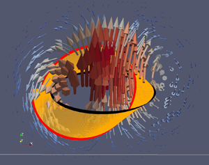
The dipole solution (3.19) is the sum of a radially oscillating part given by  $\boldsymbol {u}_{1}(r,\theta )$ and a radially monotonic part given by $\boldsymbol {u}_{2}(r,\theta )$. The azimuthal component of $\boldsymbol {u}_{1}(r,\theta )$, basically the term ${\rm j}_1(k r) \sin \theta \,\hat {\boldsymbol {\varphi }}$, is the sought LC dipole dependence mentioned in § 1. This dipole solution is, if we regard the first vorticity ball whose radius is given by the first zero of ${\rm j}_{1}(x)$ or ${\rm j}_{2}(x)$, the interior solution of the Hicks–Moffatt (Hicks Reference Hicks1899; Moffatt Reference Moffatt1969) swirling spherical vortex. Thus, the Hicks–Moffatt vortex is categorized as a 3-D vortex dipole because the number of nodal lines is given by the value of ${\ell }$, in this case ${\ell }=1$, in the vector spherical harmonics basis framework. Larger vorticity balls have been considered recently by Bogoyavlenskij (Reference Bogoyavlenskij2017) to investigate the vortex knots of these vortex solutions.
Velocity  $\boldsymbol {u}_{2}$ is a cylindrical solid-body rotation with swirl. It is the velocity field that leaves invariant the condition $\boldsymbol {\nabla }\boldsymbol {u}\,\boldsymbol {\omega } - \boldsymbol {\nabla }\boldsymbol {\omega }\,\boldsymbol {u}=\boldsymbol {0}$. Since $\boldsymbol {u}_{2}$ is a rigid motion it may be interpreted as the velocity of a (non-inertial) reference frame. This interpretation is explained in more detail in Appendix B.
Since  ${\rm j}_{0}(0)= 1$ and $\lim _{x\rightarrow 0}{{\rm j}_{1}(x)/x}= 1/3$, the constant $\hat {w}_{1}+\hat {w}_{2}$ is the velocity at the origin of the reference frame $r=0$,
 \begin{equation} \boldsymbol{u}(0) = \boldsymbol{u}_{1}(0) + \boldsymbol{u}_{2}(0) = (\hat{w}_{1} + \hat{w}_{2}) \hat{\boldsymbol{z}}. \end{equation}
Since  ${\rm j}_1(x)$ is odd and ${\rm j}_0(x)$ is even, the transformation $k\rightarrow -k$ changes the sign of the azimuthal velocity $\boldsymbol {u} \boldsymbol {\cdot } \hat {\boldsymbol {\varphi }}$ and therefore the vortex (3.19) admits two circular polarizations. We may express (3.19), using a mix of basis vectors, as
 \begin{equation} \boldsymbol{u}= \left( 3 \hat{w}_{1} \frac{{\rm j}_1(k r)}{kr} + \hat{w}_{2} \right) \left( \hat{\boldsymbol{z}} - \frac{k}{2} \rho \hat{\boldsymbol{\varphi}} \right) + 3 \hat{w}_{1} \frac{{\rm j}_{2}(k r)}{2}\hat{\boldsymbol{\theta}}. \end{equation}
Expression (3.21) makes it clear that on the spherical surfaces whose radii are the zeros  ${\rm j}_{5/2,n}$ of ${\rm j}_{2}(x)$, velocities $\boldsymbol {u}_{1}$ and $\boldsymbol {u}_{2}$ are parallel (or antiparallel) regardless of the value of their respective amplitudes $\hat {w}_{1}$ and $\hat {w}_{2}$. These spherical surfaces become stagnation surfaces, as noticed by Moffatt (Reference Moffatt1969), when the ratio between the amplitudes $\hat {w}_{2}$ and $\hat {w}_{1}$ satisfies
 \begin{equation} \frac{\hat{w}_{2}}{\hat{w}_{1}} ={-} 3 \, \frac{{\rm j}_{1}( {\rm j}_{{5}/{2},n} ) }{{\rm j}_{{5}/{2},n}} ={-} {\rm j}_{0} ( {\rm j}_{{5}/{2},n} ), \end{equation}
where the last equality is found using the identity
 \begin{equation} {\rm j}_0(x) + {\rm j}_2(x) = 3 \,\frac{{\rm j}_1(x)}{x}. \end{equation}
The vorticity of (3.19) is
 \begin{equation} \boldsymbol{\omega} = \boldsymbol{\omega}_{1} + \boldsymbol{\omega}_{2},\quad \boldsymbol{\omega}_{1} ={-}k \boldsymbol{u}_{1},\quad \boldsymbol{\omega}_{2} ={-}k \hat{w}_{2} \hat{\boldsymbol{z}}. \end{equation}
Therefore  $\boldsymbol {u}_{1}$ is a Trkalian flow
 \begin{equation} \boldsymbol{\nabla} \times \boldsymbol{u}_{1} ={-} k \boldsymbol{u}_{1}, \end{equation}
and hence a Beltrami flow as well,  $\boldsymbol {\omega }_{1} \times \boldsymbol {u}_{1} = \boldsymbol {0}$, with helicity density
 \begin{equation} \boldsymbol{\omega}_{1} \boldsymbol{\cdot} \boldsymbol{u}_{1} ={-} k\boldsymbol{u}_{1} \boldsymbol{\cdot} \boldsymbol{u}_{1} ={-} k u_{1}^2(r,\theta), \end{equation}
whereas the Lamb vector and helicity density for the flow  $\boldsymbol {u}_{2}$ are
 \begin{equation} \boldsymbol{\omega}_{2} \times \boldsymbol{u}_{2} ={-}k^2 \frac{\hat{w}_{2}^{2}}{2} \rho \hat{\boldsymbol\rho},\quad \boldsymbol{\omega}_{2} \boldsymbol{\cdot} \boldsymbol{u}_{2} ={-}k \hat{w}_{2}^2. \end{equation}
Therefore  $\boldsymbol {\omega }_{2} \times \boldsymbol {u}_{2}$ only vanishes along the $\hat {\boldsymbol {z}}$-axis, and $\boldsymbol {u}_{2}$ has constant helicity density. Explicitly, the vorticity field of (3.19) is
 \begin{align} \boldsymbol{\omega}(r,\theta) &= \boldsymbol{\omega}_{1}(r,\theta) + \boldsymbol{\omega}_{2}(r,\theta) \nonumber\\ &={-} 3 \hat{w}_{1} k \left\{\frac{{\rm j}_1(k r)}{kr}\cos\theta \, \hat{\boldsymbol{r}} +\left(\frac{{\rm j}_{2}(k r)}{2} - \frac{{\rm j}_{1}(k r)}{k r} \right) \sin\theta \,\hat{\boldsymbol{\theta}} -\frac{{\rm j}_1(k r)}{2}\sin\theta \,\hat{\boldsymbol{\varphi}}\right\} \nonumber\\ &\quad -\hat{w}_{2} k ( \cos\theta \,\hat{\boldsymbol{r}} - \sin\theta\, \hat{\boldsymbol{\theta}} ). \end{align}
The vorticity at the origin  $r=0$ is $\boldsymbol {\omega }(0)=-(\hat {w}_{1} + \hat {w}_{2}) k \hat {\boldsymbol {z}}$. The vorticity field (3.28) has no surfaces of zero amplitude because $\boldsymbol {\omega } \boldsymbol {\cdot } \hat {\boldsymbol {\varphi }} = 0$ only occurs at the zeros $kr={\rm j}_{3/2,n}$ of ${\rm j}_{1}(kr)$, and on these spherical surfaces the condition $\boldsymbol {\omega }\boldsymbol {\cdot } \hat {\boldsymbol {r}} = 0$ necessarily implies $\hat {w}_{2}=0$ so that $\boldsymbol {\omega }({\rm j}_{3/2,n},\theta ) = (3/2) \hat {w}_{1} k {\rm j}_{0}({\rm j}_{3/2,n}) \sin \theta \,\hat {\boldsymbol {\theta }}$, which has no zeros except at the poles $\theta =0,{\rm \pi}$. Thus, if a piecewise vorticity vortex is constructed by assembling an interior vorticity ball with this vorticity to an exterior irrotational flow through a single boundary separating the rotational from the irrotational flow, it must necessarily imply vorticity discontinuities at the vortex boundary. These vorticity jumps, however, may be avoided by imposing different radial boundaries for the different vorticity terms. This problem is not solved in this work and is left for future research.
In the limit  $x \rightarrow 0$ we have the following Taylor series expansions,
 \begin{equation} {\rm j}_{0}(x) \sim 1 - \frac{x^2}{6},\quad {\rm j}_{1}(x) \sim \frac{x}{3},\quad \frac{{\rm j}_{1}(x)}{x} \sim \frac{1}{3} - \frac{x^2}{30}, \end{equation}
and therefore in the limit  $k r \rightarrow 0$ the vortex velocity
 \begin{equation} \boldsymbol{u}(r,\theta) \sim{-} \hat{w}_{1} k^2 \left( \frac{r^2\cos\theta}{10} \hat{\boldsymbol{r}} - \frac{r^2\sin\theta}{5}\hat{\boldsymbol{\theta}} \right), \end{equation}
which is the vortex  $\boldsymbol {u}_{a}(r,\theta )$ (3.6) with $w_{a}=0$, $d_{a}=0$ and $\chi _{a}=\hat {w}_{1} k^2$. Thus, as noticed by Scase & Terry (Reference Scase and Terry2018), Hill's spherical ring is a particular case of Hicks–Moffatt swirling spherical vortex in the limit of vanishing wavenumber.
We record also the Laplacian of the velocity (3.19),
 \begin{align} \nabla^2\boldsymbol{u}(r,\theta) &= \nabla^2\boldsymbol{u}_{1}(r,\theta) + \nabla^2\boldsymbol{u}_{2}(r,\theta) \nonumber\\ &={-} 3 \hat{w}_{1} k \left\{\frac{{\rm j}_1(k r)}{kr} \cos\theta \, \hat{\boldsymbol{r}} +\left( \frac{{\rm j}_{2}(k r)}{2} - \frac{{\rm j}_{1}(k r)}{k r} \right) \sin\theta \,\hat{\boldsymbol{\theta}} -\frac{{\rm j}_1(k r)}{2} \sin\theta \,\hat{\boldsymbol{\varphi}}\right\} \nonumber\\ &\quad - \hat{w}_{2} k ( \cos\theta \,\hat{\boldsymbol{r}} - \sin\theta \,\hat{\boldsymbol{\theta}} ). \end{align}
 We now provide the streamfunctions  $\boldsymbol {\psi }_{i}$ satisfying $\boldsymbol {u}_{i} = \boldsymbol {\nabla }\times \boldsymbol {\psi }_{i}$ with the divergenceless constraint $\boldsymbol {\nabla }\boldsymbol {\cdot }\boldsymbol {\psi }_{i}=0$ for the velocity fields $\boldsymbol {u}_{1}$ and $\boldsymbol {u}_{2}$. Given the mathematical identity
 \begin{equation} \nabla^2 \boldsymbol{\chi} ={-}\boldsymbol{\nabla}\times\boldsymbol{\nabla}\times\boldsymbol{\chi} + \boldsymbol{\nabla} (\boldsymbol{\nabla}\boldsymbol{\cdot}\boldsymbol{\chi}), \end{equation}
for any vector field  $\boldsymbol {\chi }$, it is immediately deduced that $\boldsymbol {\psi }_{1}$ and ${\boldsymbol {\psi }}_{2}$ satisfy
 \begin{equation} \nabla^2 \boldsymbol{\psi}_{i} ={-}\boldsymbol{\omega}_{i}. \end{equation}
Therefore  $\boldsymbol {\psi }_{1} = \boldsymbol {\omega }_{1}/{k^2} = -\boldsymbol {u}_{1}/{k}$, or
 \begin{equation} \boldsymbol{u}_{1} ={-} k \boldsymbol{\psi}_{1},\quad \boldsymbol{\omega}_{1} = k^2 \boldsymbol{\psi}_{1}. \end{equation}
Thus,  $\boldsymbol {\psi }_{1}$ and all their rotational fields satisfy the vector Helmholtz equation,
 \begin{equation} \nabla^2 \boldsymbol{\psi}_{1} + k^2 \boldsymbol{\psi}_{1} = \boldsymbol{0},\quad \nabla^2 \boldsymbol{u}_{1} + k^2 \boldsymbol{u}_{1} = \boldsymbol{0},\quad \nabla^2 \boldsymbol{\omega}_{1} + k^2 \boldsymbol{\omega}_{1} = \boldsymbol{0}, \quad \ldots . \end{equation}
On the other hand,  $\boldsymbol {\psi }_{2}$ satisfies
 \begin{equation} \boldsymbol{\psi}_{2} = \frac{\hat{w}_{2}}{2} \left(\frac{k}{5} r^2 ( \cos\theta \,\hat{\boldsymbol{r}} - 2 \sin\theta \,\hat{\boldsymbol{\theta}} )+ r \sin\theta \, \hat{\boldsymbol{\varphi}} \right). \end{equation}
 Since both  $\boldsymbol {u}_{1}$ and $\boldsymbol {u}_{2}$ independently, as well as their sum, satisfy the vorticity steadiness condition, they also satisfy
 \begin{align} \boldsymbol{\nabla} \times ( \boldsymbol{\omega} \times \boldsymbol{u} ) = \boldsymbol{\nabla} \times ( (\boldsymbol{\omega}_{1} + \boldsymbol{\omega}_{2}) \times (\boldsymbol{u}_{1} + \boldsymbol{u}_{2}) ) = \boldsymbol{\nabla} \times ( \boldsymbol{\omega}_{1} \times \boldsymbol{u}_{2} - \boldsymbol{u}_{1} \times \boldsymbol{\omega}_{2} ) = 0, \end{align}
which is another way of proving that the flow solutions  $\boldsymbol {u}_{1}$ and $\boldsymbol {u}_{1}$ are linearly superposable. This means that there is a potential $\varXi (r,\theta )$ for the Lamb vector $\boldsymbol {\omega } \times \boldsymbol {u}$ such that
 \begin{equation} \boldsymbol{\omega} \times \boldsymbol{u} = \boldsymbol{\nabla}\varXi. \end{equation}
A simple potential is
 \begin{equation} \varXi (r , \theta) ={-}\frac{\hat{w}_{2}}{4} k r ( 3 \hat{w}_{1} {\rm j}_{1}(k r) + \hat{w}_{2} k r ) \sin^2\theta. \end{equation}
 Since the components of  $\boldsymbol {u}$ do not depend on $\varphi$, the components of $\boldsymbol {\omega }$ do not either, and therefore $\hat {\boldsymbol {\varphi }}\boldsymbol {\cdot } (\boldsymbol {\omega } \times \boldsymbol {u})$, the component along $\varphi$ of the Lamb vector, vanishes. From Lagrange's acceleration formula,
 \begin{equation} \boldsymbol{a} = \frac{\partial \boldsymbol{u}}{\partial t} + \boldsymbol{\omega} \times \boldsymbol{u} + \frac{1}{2}\boldsymbol{\nabla}( \boldsymbol{u} \boldsymbol{\cdot} \boldsymbol{u}), \end{equation}
we readily obtain that
 \begin{equation} \boldsymbol{a} \boldsymbol{\cdot} \hat{\boldsymbol{\varphi}} = 0, \end{equation}
and see that the flow has no azimuthal acceleration. Since in spherical coordinates  $\boldsymbol {a} \boldsymbol {\cdot } \hat {\boldsymbol {\varphi }}= r \ddot {\varphi } \sin \theta + 2 \dot {r}\dot {\varphi }\sin \theta + 2 r \dot {\theta }\dot {\varphi }\cos \theta$, and in cylindrical coordinates $\boldsymbol {a} \boldsymbol {\cdot } \hat {\boldsymbol {\varphi }}=\rho \ddot {\varphi } + 2 \dot {\rho } \varphi$, we obtain as an integral of motion
 \begin{equation} r^2 \dot{\varphi} \sin^2\theta = r^2_{0} \dot{\varphi}_{0} \sin^2\theta_0,\quad \rho^2 \dot{\varphi} = \rho^2_{0}\dot{\varphi}_{0}, \end{equation}
and therefore an integral of motion for a fluid particle  $\rho ^2(t) \dot {\varphi }(t) = \rho ^2_{0}\dot {\varphi }_{0}$, which represents the conservation of angular momentum
 \begin{equation} \boldsymbol{L} \equiv \boldsymbol{r} \times \boldsymbol{u} \end{equation}
along  $\hat {\boldsymbol {z}}$, that is, defining $L_{z} \equiv \boldsymbol {L}\boldsymbol {\cdot }\hat {\boldsymbol z}$ and using a dot $(\dot {~})$ for the material time derivative,
 \begin{equation} \dot{\boldsymbol{L}} \boldsymbol{\cdot} \hat{\boldsymbol{z}} = \dot{\overline{\boldsymbol{L} \boldsymbol{\cdot} \hat{\boldsymbol{z}}}} = \dot{L_{z}}= \dot{\overline{\rho^2 \dot{\varphi}}} = 0,\quad \dot{\boldsymbol{L}} \boldsymbol{\cdot} \hat{\boldsymbol{\rho}} ={-}\frac{z}{\rho} \dot{\overline{\rho^2 \dot{\varphi}}} = 0, \end{equation}
where we note that  $\dot {\boldsymbol {L}} \boldsymbol {\cdot } \hat {\boldsymbol {\rho }} \neq \dot {\overline {\boldsymbol {L} \boldsymbol {\cdot } \hat {\boldsymbol {\rho }}}}$. The field $L_z(r,\theta )$ is
 \begin{equation} L_{z}(r,\theta) ={-}\frac{\sin^2\theta}{2} r ( 3 \hat{w}_1 {\rm j}_{1}(k r) + \hat{w}_2 k r ), \end{equation}
which implies the relation with the Lamb vector potential
 \begin{equation} \varXi = \tfrac{1}{2} k \hat{w}_2 L_{z}. \end{equation}
 In these steady flow solutions, a potential  $P(r,\theta )$, or negative pressure, of the acceleration field $\boldsymbol {a}$ such that $\boldsymbol {a}=\boldsymbol {\nabla } P$ is easily obtained from (3.38), (3.39) and (3.40), resulting in
 \begin{equation} P = \varXi + \tfrac{1}{2} \boldsymbol{u}\boldsymbol{\cdot}\boldsymbol{u}. \end{equation}
4. Multipolar vortices
We now deal with the general multipolar vortex whose velocity  $\boldsymbol {u}_{{\ell } m}(r,\theta,\varphi )$, given by (2.5), already satisfies the isochoric condition $\boldsymbol {\nabla }\boldsymbol {\cdot }\boldsymbol {u}_{{\ell } m}=0$. The vector spherical harmonics may be expressed as
 \begin{gather} \boldsymbol{Y}_{{\ell}}^{m}(\theta,\varphi) = {\rm Y}_{{\ell}}^{m}(\theta,\varphi) \hat{\boldsymbol{r}}, \end{gather}
 \begin{gather}\boldsymbol{\varPsi }_{{\ell}}^{m}(\theta,\varphi) = \left( m \cot\theta \, {\rm Y}_{{\ell}}^{m}(\theta,\varphi) + \hat{\varGamma}_{{\ell}}^{m} \frac{{\rm Y}_{{\ell}}^{m+1} (\theta,\varphi)}{{\rm e}^{{\rm i}\varphi}}\right) \hat{\boldsymbol{\theta}}+ {\rm i} m \csc\theta \, {\rm Y}_{{\ell}}^{m}(\theta,\varphi) \hat{\boldsymbol{\varphi}}, \end{gather}
 \begin{gather}\boldsymbol{\varPhi }_{{\ell}}^{m}(\theta,\varphi) ={-}{\rm i} m \csc\theta \, {\rm Y}_{{\ell}}^{m}(\theta,\varphi) \hat{\boldsymbol{\theta}} + \left( m \cot\theta \, {\rm Y}_{{\ell}}^{m}(\theta,\varphi) + \hat{\varGamma}_{{\ell}}^{m} \frac{{\rm Y}_{{\ell}}^{m+1} (\theta,\varphi)}{{\rm e}^{{\rm i}\varphi}}\right) \hat{\boldsymbol{\varphi}}, \end{gather}
where
 \begin{equation} \hat{\varGamma}_{{\ell}}^{m} \equiv \sqrt{{\ell}-m} \, \sqrt{{\ell}+m+1}. \end{equation}
 Henceforth, to simplify the notation, we will often omit the indices  $\{ {\ell }, m\}$. The vorticity is
 \begin{align} \boldsymbol{\omega} &= \xi(r) \boldsymbol{Y} + \eta(r) \boldsymbol{\varPsi} + \zeta(r) \boldsymbol{\varPhi} \nonumber\\ &={-}{\ell}({\ell}+1)\frac{w}{r} \boldsymbol{Y}- \frac{r w'+ w}{r} \boldsymbol{\varPsi} + \frac{r ( r u'' + 4 u' ) - ({\ell}-1)({\ell}+2) u}{{\ell}({\ell}+1)r} \boldsymbol{\varPhi}. \end{align}
We note from (4.3) that, due to the term  $({\ell }-1)$, only in the particular case ${\ell }=1$ do the vorticity components depend on $u'(r)$ and $u''(r)$ but not on $u(r)$. This fact allowed the introduction of the rigid motion $\boldsymbol {u}_2$ as a superposable velocity in the vortex dipole solution (3.18). This property, which is absent for modes ${\ell }>1$, is responsible for the vortex dipole being a special case different from higher-order multipoles.
The Lamb vector  ${\boldsymbol l}_{l m}(r,\theta,\varphi )$, and their components relative to the vector spherical harmonics basis $\{ \boldsymbol {Y}, \boldsymbol {\varPsi }, \boldsymbol {\varPhi } \}$, are
 \begin{align} \boldsymbol{l} &= (\eta w - \zeta v ) \varPhi^2 \hat{\boldsymbol{r}} + ( \zeta u - \xi w ) {\rm Y} \boldsymbol{\varPsi} + ( \xi v - \eta u ) {\rm Y} \boldsymbol{\varPhi} \nonumber\\ &= l_{\rm Y}(r) \frac{\varPhi^2}{\rm Y} \boldsymbol{Y} + l_{\varPsi}(r) {\rm Y}\boldsymbol{\varPsi} + l_{\varPhi}(r) {\rm Y}\boldsymbol{\varPhi}, \end{align}
where  $\{ l_{\rm Y} , l_{\varPsi } , l_{\varPhi } \} \equiv \{ \eta w - \zeta v , \zeta u - \xi w , \xi v - \eta u \}$ are the terms with radial dependence in the components of the Lamb vector relative to the basis $\{ \boldsymbol {Y}, \boldsymbol {\varPsi } , \boldsymbol {\varPhi } \}$, and $\varPhi ^2=\boldsymbol {\varPhi }\boldsymbol {\cdot }\boldsymbol {\varPhi } =\varPsi ^2=\boldsymbol {\varPsi }\boldsymbol {\cdot }\boldsymbol {\varPsi }$. From (4.4) we obtain the curl of the Lamb vector,
 \begin{align} \boldsymbol{\nabla} \times \boldsymbol{l} &= {\rm Y} ( \boldsymbol{\nabla} \times ( l_{\varPsi} \boldsymbol{\varPsi} + l_{\varPhi} \boldsymbol{\varPhi} ) ) + l_{\varPhi} \frac{\varPhi^2}{r} \hat{\boldsymbol{r}} + l_{\rm Y} \boldsymbol{\nabla} {\varPhi}^2 \times \hat{\boldsymbol{r}} \nonumber\\ &= \frac{l_{\varPhi}}{r} ( \varPhi^2 - {\ell}({\ell}+1) {\rm Y}^2 ) \hat{\boldsymbol{r}} - \left( l'_{\varPhi} + \frac{l_{\varPhi}}{r} \right) {\rm Y} \boldsymbol{\varPsi} + \left( l'_{\varPsi} + \frac{l_{\varPsi}}{r} \right) {\rm Y} \boldsymbol{\varPhi} + l_{\rm Y} \boldsymbol{\nabla} {\varPhi}^2 \times \hat{\boldsymbol{r}}. \end{align}
From  $(\boldsymbol {\nabla } \times \boldsymbol {l}) \boldsymbol {\cdot } \hat {\boldsymbol {r}} = 0$, and since $\varPhi ^2 \neq {\ell }({\ell }+1) {\rm Y}^2$ for integers $\ell \geq 0$, we readily obtain $l_{\varPhi }(r)=0$, which implies
 \begin{equation} w(r) = \frac{k r}{{\ell}({\ell}+1)} u(r), \end{equation}
and hence  $\boldsymbol {\nabla }\times \boldsymbol {l}=\boldsymbol {0}$ simplifies to
 \begin{equation} \left( l'_{\varPsi} + \frac{l_{\varPsi}}{r} \right) {\rm Y} \boldsymbol{\varPhi} + l_{\rm Y} \boldsymbol{\nabla} {\varPhi}^2 \times \hat{\boldsymbol{r}}= \boldsymbol{0}. \end{equation}
 Now we analyse two sets of steady solutions ( $\boldsymbol {\nabla }\times \boldsymbol {l}=\boldsymbol {0}$), namely non-Beltrami ( $\boldsymbol {l}\neq \boldsymbol {0}$) and Beltrami ( $\boldsymbol {l}=\boldsymbol {0}$) flows.
4.1. Non-Beltrami flows
We start with non-Beltrami flows. Condition (4.7) implies that both  $l_{\rm Y}(r)$ and $l_{\varPsi }(r)$ must be different from zero. Projection $(\boldsymbol {\nabla } \times \boldsymbol {l}) \boldsymbol {\cdot } {\boldsymbol {\varPsi }} = 0$ implies that $l_{\rm Y} (\boldsymbol {\nabla } {\varPhi }^2 \times \hat {\boldsymbol {r}} ) \boldsymbol {\cdot } \boldsymbol {\varPsi } =0$. Therefore $\boldsymbol {\nabla } {\varPhi }^2 \times \hat {\boldsymbol {r}}$ must be parallel to $\boldsymbol {\varPhi }$ and, in order to satisfy the third condition $(\boldsymbol {\nabla } \times \boldsymbol {l}) \boldsymbol {\cdot } {\boldsymbol {\varPhi }} = 0$, one must have ${\rm Y} \boldsymbol {\varPhi } = c_0 r \boldsymbol {\nabla } {\varPhi }^2 \times \hat {\boldsymbol {r}}$ for a constant $c_0$. This implies that ${\rm Y} {\boldsymbol {r}} \times \boldsymbol {\nabla } {\rm Y} = -c_{0} \varPhi {\boldsymbol {r}} \times \boldsymbol {\nabla } {\varPhi }$, hence $\boldsymbol {\nabla } {\rm Y}^{2} = -c_{0} \boldsymbol {\nabla } {\varPhi }^2$, and therefore ${\rm Y}^2 + c_0 \varPhi ^2=c_1$, for a constant $c_1$. This condition is satisfied when ${\ell } = 1$, with $c_1 \neq 0$ in the cases $m = \pm 1$, and $c_1 = 0$ in the case $m = 0$, since
 \begin{align} ( {\rm Y}_{1}^{0} )^2 = \frac{3}{4{\rm \pi}} \cos^2\theta,\quad ( {\varPhi}_{1}^{0} )^2 = \frac{3}{4{\rm \pi}} \sin^2\theta,\quad ( {\rm Y}_{1}^{{\pm} 1} )^2 ={-} ( {\varPhi}_{1}^{{\pm} 1} )^2 = \frac{3}{8{\rm \pi}} {\rm e}^{{\pm} 2{\rm i} \varphi} \sin^2\theta. \end{align}
 For  ${\ell }=1$, a solution exists with non-zero Lamb components such that, relative to the basis $\{ \boldsymbol {Y}, \boldsymbol {\varPsi }, \boldsymbol {\varPhi } \}$, whose rotational is zero and therefore is a steady solution of the vorticity equation. The solutions to this case have already been discussed in § 3.
For modes  ${\ell }>1$, the condition ${\rm Y}^2 + c_0 \varPhi ^2=c_1$ is satisfied (with $c_1=0$) in the cases $m = \pm {\ell }$. In these cases, solutions $u(r)$ to (4.7) exist as $r^{{\ell }-1}$. The velocity components, omitting a constant factor, are therefore
 \begin{equation} u(r) = (k r)^{{\ell}-1},\quad v(r) = \frac{(k r)^{{\ell}-1}}{{\ell}},\quad w(r) = \frac{(k r)^{{\ell}}}{{\ell}}. \end{equation}
The corresponding vorticity solutions are
 \begin{equation} \boldsymbol{\omega}_{{\ell} \pm{\ell}}(r,\theta,\varphi) = k^{{\ell}} r^{{\ell}-1} (\sin\theta)^{{\ell}-1} ( \sin\theta \,\hat{\boldsymbol{r}} + \cos\theta \, \hat{\boldsymbol{\theta}} \pm {\rm i} \hat{\boldsymbol{\varphi}} ) {\rm e}^{{\pm}{\rm i}{\ell}\varphi}. \end{equation}
These solutions have vanishing Laplacian  ${\nabla }^2 \boldsymbol {u} = \boldsymbol {0}$, and therefore, since $\boldsymbol {\nabla }\boldsymbol {\cdot }\boldsymbol {u}=0$, the vorticity is irrotational, $\boldsymbol {\nabla } \times \boldsymbol {\omega } = \boldsymbol {0}$, and hence the vorticity Laplacian vanishes as well, ${\nabla }^2 \boldsymbol {\omega } = \boldsymbol {0}$. We note, however, that these velocity and vorticity solutions are, for ${\ell }>1$, strictly complex-valued functions. The helicity density vanishes also, $\boldsymbol {\omega } \boldsymbol {\cdot } \boldsymbol {u} = 0$, while the Lamb vector, $\boldsymbol {l}\equiv \boldsymbol {\omega } \times \boldsymbol {u}$, is
 \begin{equation} \boldsymbol{l}_{{\ell} \pm{\ell}}(r,\theta,\varphi) = k^{2{\ell}} r^{2{\ell}-1} (\sin\theta)^{2{\ell}-1} ( \sin\theta \,\hat{\boldsymbol{r}} + \cos\theta\,\hat{\boldsymbol{\theta}} \pm {\rm i} \hat{\boldsymbol{\varphi}} ) {\rm e}^{{\pm} 2{\rm i}{\ell}\varphi}. \end{equation}
4.2. Beltrami flows
We turn now to Beltrami flows  $\boldsymbol {l}(r,\theta,\varphi )=\boldsymbol {0}$. The term $\boldsymbol {l}\boldsymbol {\cdot }\hat {\boldsymbol {\theta }}$ is
 \begin{equation} \boldsymbol{l}\boldsymbol{\cdot}\hat{\boldsymbol{\theta}} = \frac{u}{{\ell} ({\ell}+1)r} [ r^2 u'' + 4 r u' + u (k^2 r^2 -({\ell}-1)({\ell}+2) ) ], \end{equation}
which, apart from the null solution  $u(r)=0$, has the solution
 \begin{equation} u(r) = c_{1} \frac{{\rm j}_{{\ell}}(k r)}{k r} + c_{2} \frac{{\rm y}_{{\ell}}(k r)}{k r}. \end{equation}
Omitting the term with a singularity at  $r=0$, the solution of the multipolar ${\ell }>1$ vortex velocity is therefore
 \begin{align} \boldsymbol{u}_{{\ell} m}^{k}(r,\theta,\varphi) &= \frac{{\rm j}_{{\ell}}(k r)}{k r} \boldsymbol{Y}_{{\ell}}^{m}(\theta,\varphi) + \left( \frac{{\rm j}_{{\ell}}(k r)}{{\ell} k r} - \frac{{\rm j}_{{\ell}+1}(k r)}{{\ell}({\ell}+1)} \right) \boldsymbol{\varPsi }_{{\ell}}^{m}(\theta,\varphi) \nonumber\\ &\quad +\frac{{\rm j}_{{\ell}}(k r)}{{\ell}({\ell}+1)} \boldsymbol{\varPhi }_{{\ell}}^{m}(\theta,\varphi). \end{align}
In (4.14) the superscript  $k$ is introduced to explicitly express the dependence on the wavenumber $k$, whose amplitude provides the relative spatial scale of the velocity field and whose sign defines one of the two possible velocity polarizations. This is so because ${\rm j}_{\ell }(-x)=(-1)^{\ell } {\rm j}(x)$, that is, ${\rm j}_{\ell }(x)$ and ${\ell }$ have the same parity, and the parity of the $\boldsymbol {\varPhi }$ component of velocity is opposite to the parities of the $\boldsymbol {Y}$ and $\boldsymbol {\varPsi }$ components of velocity. Explicitly we may express this as
 \begin{align} ({-}1)^{{\ell}+1} \boldsymbol{u}_{{\ell} m}^{{-}k}(r,\theta,\varphi) &= \frac{{\rm j}_{{\ell}}(k r)}{k r} \boldsymbol{Y}_{{\ell}}^{m}(\theta,\varphi) +\left( \frac{{\rm j}_{{\ell}}(k r)}{{\ell} k r} - \frac{{\rm j}_{{\ell}+1}(k r)}{{\ell}({\ell}+1)} \right) \boldsymbol{\varPsi }_{{\ell}}^{m}(\theta,\varphi) \nonumber\\ &\quad - \frac{{\rm j}_{{\ell}}(k r)}{{\ell}({\ell}+1)} \boldsymbol{\varPhi }_{{\ell}}^{m}(\theta,\varphi). \end{align}
 As happens with the Beltrami flow component of the vortex dipole flow, one may define the streamfunction  $\boldsymbol {u}_{{\ell } m}^{k}(r,\theta,\varphi ) = \boldsymbol {\nabla } \times \boldsymbol {\psi }_{{\ell } m}^{k}(r,\theta,\varphi )$ with the constraint $\boldsymbol {\nabla } \boldsymbol {\cdot } \boldsymbol {\psi }_{{\ell } m}^{k}=0$ and find that $\boldsymbol {\psi }_{{\ell } m}^{k} = -k^{-1} \boldsymbol {u}_{{\ell } m}^{k}$. Then the vorticity is simply $\boldsymbol {\omega }_{{\ell } m}^{k}= -k \boldsymbol {u}_{{\ell } m}^{k}$. Thus, $\boldsymbol {\psi }_{{\ell } m}^{k}$ and all their curls (as $\boldsymbol {u}_{{\ell } m}^{k}$, $\boldsymbol {\omega }_{{\ell } m}^{k}$, $\boldsymbol {\chi }_{{\ell } m}^{k}$, …) satisfy the vector Helmholtz equation
 \begin{equation} (\nabla^2 + k^2) ( \boldsymbol{\nabla}\times )^{n} \boldsymbol{\psi}_{{\ell} m}^{k} = \boldsymbol{0},\quad n=0,1,2,\ldots . \end{equation}
 Since  $\boldsymbol {u}_{{\ell } m}^{k}$ is a Trkalian flow, it satisfies the vector Helmholtz equation, ${\nabla }^2\boldsymbol {u}= -k^2 \boldsymbol {u}$. Once it is known that the velocity flow solution $\boldsymbol {u}$ must be a Trkalian flow, there is a shortcut to obtain $\boldsymbol {u}$ by noticing that, because of (A4), the Helmholtz equation ${\nabla }^2 \boldsymbol {u} = -k^2 (u\boldsymbol {Y}+v\boldsymbol {\varPsi }+w\boldsymbol {\varPhi })$ implies that $w \boldsymbol {\varPhi }$ satisfies the vector Helmholtz equation as well, ${\nabla }^2 ( w \boldsymbol {\varPhi } ) = -k^2 w \boldsymbol {\varPhi }$. Because of (A4c) the component $w(r)$ satisfies the Bessel equation $( r^2 w'(r) )' + ( k^2 r^2 - {\ell }({\ell }+1)) w(r) = 0$ whose solutions are the spherical Bessel functions ${\rm j}_{{\ell }}(kr)$ and ${\rm y}_{{\ell }}(kr)$. Hence, from $l_{\varPhi }=0$ (4.6), we deduce $u(r)={\ell }({\ell }+1) w(r)/(kr)$, and finally from the isochoric condition (2.2) we obtain $v(r)=(2 u(r)+r u'(r) )/({\ell }({\ell }+1))$.
We end this section by noting that, since the vorticity field  $\boldsymbol {\omega }_{{\ell } m}^{k}(\boldsymbol {x})$ satisfies the vector Helmholtz equation, the time-dependent velocity and vorticity fields
 \begin{equation} \tilde{\boldsymbol{u}}_{{\ell} m}^{k}(\boldsymbol{x},t) \equiv \boldsymbol{u}_{{\ell} m}^{k}(\boldsymbol{x}) {\rm e}^{-\nu k^2 t} \quad {\rm and} \quad \tilde{\boldsymbol{\omega}}_{{\ell} m}^{k}(\boldsymbol{x},t) \equiv \boldsymbol{\omega}_{{\ell} m}^{k}(\boldsymbol{x}) {\rm e}^{-\nu k^2 t}, \end{equation}
where  $\nu$ is a constant diffusivity, satisfy the Navier–Stokes vorticity equation for isochoric flows
 \begin{equation} \frac{\partial\tilde{\boldsymbol{\omega}}_{{\ell} m}^{k}}{\partial t} + \boldsymbol{\nabla} \times ( \tilde{\boldsymbol{\omega}}_{{\ell} m}^{k} \times \tilde{\boldsymbol{u}}_{{\ell} m}^{k} ) = \nu \nabla^2 \tilde{\boldsymbol{\omega}}_{{\ell} m}^{k}, \end{equation}
which for Beltrami flows is reduced to
 \begin{equation} \frac{\partial\tilde{\boldsymbol{\omega}}_{{\ell} m}^{k}}{\partial t} ={-} \nu k^2 \tilde{\boldsymbol{\omega}}_{{\ell} m}^{k}. \end{equation}
The non-Beltrami solutions given in § 4.1 trivially satisfy the Navier–Stokes vorticity equation since the Laplacian of the vorticity vanishes.
5. Irrotational flow
Finite-size vortex flow configurations often separate the vortex solution into an interior rotational flow and an exterior irrotational flow. This approach requires the specification of irrotational flow matching boundary conditions at the vortex boundary and hence the interest in providing the irrotational velocity components in the vector spherical harmonics basis. This solution is simple and is provided here in the general multipolar case. We introduce three scalar radial functions  $\{ \bar {u}_{{\ell } m}(r), \bar {v}_{{\ell } m}(r), \bar {w}_{{\ell } m}(r) \}$ in such a way that the irrotational flow in the vector spherical harmonics basis is
 \begin{equation} \bar{\boldsymbol{u}}_{{\ell} m}(r,\theta,\varphi) = \bar{u}_{{\ell} }(r) \boldsymbol{Y}_{{\ell}}^{m}(\theta,\varphi) + \bar{v}_{{\ell} }(r) \boldsymbol{\varPsi }_{{\ell}}^{m}(\theta,\varphi) + \bar{w}_{{\ell} }(r) \boldsymbol{\varPhi }_{{\ell}}^{m}(\theta,\varphi). \end{equation}
Properties (A3) applied to  $\boldsymbol {\nabla } \times \bar {\boldsymbol {u}}_{{\ell } m}=\boldsymbol {0}$ imply $\bar {w}_{{\ell }}(r)=0$ and $\bar {u}_{{\ell }}(r) = ( r \bar {v}_{{\ell }}(r))'$. Thus we may introduce the radial component of the potential $R_{{\ell }}(r)$ and identify $\bar {u}_{{\ell }}(r) = R'_{{\ell }}(r)$ and $\bar {v}_{{\ell }}(r) = R_{{\ell }}(r)/r$. Since $\bar {\boldsymbol {u}}_{{\ell } m}= \boldsymbol {\nabla } \phi$ implies
 \begin{equation} \bar{\boldsymbol{u}}_{{\ell} m}(r,\theta,\varphi) = R'_{{\ell}}(r) \boldsymbol{Y}_{{\ell}}^{m}(\theta,\varphi) + \frac{R_{{\ell}}(r)}{r} \boldsymbol{\varPsi }_{{\ell}}^{m}(\theta,\varphi), \end{equation}
the irrotational flow potential is  $\phi (r,\theta,\varphi )= R_{{\ell }}(r) {\rm Y}_{{\ell }}^{m}(\theta,\varphi )$. For isochoric flows $\boldsymbol {\nabla } \boldsymbol {\cdot } \bar {\boldsymbol {u}} = {\nabla }^2 \phi = 0$, so that the radial part of the potential is
 \begin{equation} R_{{\ell}}(r) = a_1 r^{\ell} + a_2 r^{-{\ell}-1}, \end{equation}
where  $\{ a_{1}, a_{2} \}$ are arbitrary constants. Solution (5.3) may also be obtained from the isochoric condition (2.2). The velocity components are therefore
 \begin{equation} \bar{u}(r) = a_1 {\ell} r^{{\ell}-1} - a_2 ({\ell}+1) r^{-{\ell}-2},\quad \bar{v}(r) = a_1 r^{{\ell}-1} + a_2 r^{-{\ell}-2},\quad \bar{w}(r) = 0, \end{equation}
where the constants  $\{ a_{1}, a_{2} \}$ must be used for matching boundary conditions with the inner rotational flow.
6. Piecewise vortices
6.1. The piecewise dipole vortex mode ${\ell }=1$

In the case of the vortex dipole  ${\ell } = 1$, we impose continuity of the velocity at the spherical surface $k r = \varrho _0$, that is $\boldsymbol {u}_{1 0}(\varrho _{0}/k,\theta,\varphi ) = \bar {\boldsymbol {u}}_{1 0}(\varrho _{0}/k,\theta,\varphi )$, which using (5.4a–c) may be written as
 \begin{equation} \boldsymbol{u}_{1 0}(\varrho_{0}/k,\theta,\varphi) = \left( \hat{a}_{1} - \frac{2 \hat{a}_{2}}{(\varrho_{0}/k)^3} \right) \cos\theta \,\hat{\boldsymbol{r}} - \left( \hat{a}_{1} + \frac{ \hat{a}_{2}}{(\varrho_{0}/k)^3} \right) \sin\theta \, \hat{\boldsymbol{\theta}}, \end{equation}
where  $\{ \hat {a}_{1}, \hat {a}_{2} \}$ are constants. Using $\boldsymbol {u}_{1 0}(\varrho _{0}/k,\theta,\varphi )$ given by (3.19) we obtain
 \begin{gather} \hat{a}_{1} ={-} \hat{w}_{1} {\rm j}_{2}(\varrho_{0}), \end{gather}
 \begin{gather}\hat{a}_{2} ={-} \frac{\hat{w}_{1}}{2} \left( \frac{\varrho_{0}}{k} \right)^{3} {\rm j}_{2}(\varrho_{0})= \frac{\hat{a}_{1}}{2} \left( \frac{\varrho_{0}}{k} \right)^{3}, \end{gather}
 \begin{gather}\hat{w}_{2} ={-}3 \hat{w}_{1} \frac{{\rm j}_{1}(\varrho_{0})}{\varrho_{0}}. \end{gather}
Relation (6.2c) is a constraint between vortex amplitude parameters  $\hat {w}_{1}$ and $\hat {w}_{2}$ that forces the vortex dipole to have zero azimuthal velocity on the spherical surface in order to match the exterior potential flow. Relations (6.2a) and (6.2b) imply that the flow at the spherical boundary,
 \begin{equation} \boldsymbol{u}_{1 0}(\varrho_{0}/k,\theta,\varphi) = \bar{\boldsymbol{u}}_{1 0}(\varrho_{0}/k,\theta,\varphi) = \tfrac{3}{2}\hat{w}_{1} {\rm j}_{2}(\varrho_{0}) \hat{\boldsymbol{\theta}}, \end{equation}
is exclusively polar. In this case, due to (6.2c), the potential  $\varXi (r,\theta )$ (3.39) vanishes at the vortex boundary $kr=\varrho _{0}$ and therefore the minus pressure ${-}p$ at the vortex boundary is given by $(1/2)\boldsymbol {u}\boldsymbol {\cdot }\boldsymbol {u}$ and is therefore continuous and equal to the constant $(9/8) \hat {w}_{1}^{2} {\rm j}_{2}(\varrho _{0})^{2}$.
The potential flow is therefore
 \begin{equation} \bar{\boldsymbol{u}}_{1 0}(r,\theta,\varphi) ={-}\hat{w}_1 {\rm j}_2(\varrho_0) \left[\left( 1 - \left( \frac{\varrho_0}{k r} \right)^3 \right) \cos\theta \,\hat{\boldsymbol{r}}- \left( 1 + \frac{1}{2}\left( \frac{\varrho_0}{k r} \right)^3 \right) \sin\theta \,\hat{\boldsymbol{\theta}}\right], \end{equation}
which as  $r \rightarrow \infty$ is a constant velocity along $\hat {\boldsymbol {z}}$ given by
 \begin{equation} \bar{\boldsymbol{u}}^{\infty}_{1 0} ={-}\hat{w}_1 {\rm j}_2(\varrho_0) ( \cos\theta \,\hat{\boldsymbol{r}} - \sin\theta \, \hat{\boldsymbol{\theta}} ) ={-}\hat{w}_1 {\rm j}_2(\varrho_0) \hat{\boldsymbol{z}}={-} \boldsymbol{U}_{0}. \end{equation}
Since this far-field potential velocity is spatially constant, a property exclusive to the mode  ${\ell }=1$, there is an unsteady velocity solution $\tilde {\boldsymbol {u}}_{1 0}(\boldsymbol {x},t)$ with vanishing far-field potential velocity such that its initial state $\tilde {\boldsymbol {u}}_{1 0}(\boldsymbol {x},t_0) \equiv \boldsymbol {u}_{1 0}(\boldsymbol {x}) + \boldsymbol {U}_{0}$ or $\tilde {\boldsymbol {u}}_{1 0}(\boldsymbol {x},t) = \boldsymbol {u}_{1 0} (\boldsymbol {x}- \boldsymbol {U}_{0} t )+ \boldsymbol {U}_{0}$, such that the dipole displaces with constant velocity $\boldsymbol {U}_{0} =\hat {w}_1 {\rm j}_2(\varrho _0) \hat {\boldsymbol {z}}$. The vorticity evolution is just a rigid translation $\tilde {\boldsymbol {\omega }}_{1 0}(\boldsymbol {x},t) = \boldsymbol {\omega }_{1 0} ( \boldsymbol {x} - \boldsymbol {U}_{0} t )$. The initial velocity field at the initial time, say $t_0=0$, is now a piecewise function given by
 \begin{align} \frac{\tilde{\boldsymbol{u}}_{1 0}(r,\theta,\varphi , t_0)}{3 \hat{w}_{1}} &= \left(\frac{{\rm j}_{1}(k r)}{kr} - \frac{{\rm j}_{1}(\varrho_0)}{\varrho_0} + \frac{{\rm j}_{2}(\varrho_{0})}{3}\right) \cos\theta \,\hat{\boldsymbol{r}} \nonumber\\ &\quad + \left( \frac{{\rm j}_{2}(k r)}{2} - \frac{{\rm j}_{1}(k r)}{kr} + \frac{{\rm j}_{1}(\varrho_0)}{\varrho_0} - \frac{{\rm j}_{2}(\varrho_{0})}{3} \right) \sin\theta \, \hat{\boldsymbol{\theta}} \nonumber\\ &\quad + \left(-\frac{{\rm j}_{1}(k r)}{2} + \frac{{\rm j}_{1}(\varrho_0)}{2} \frac{kr}{\varrho_0}\right) \sin\theta \,\hat{\boldsymbol{\varphi}},\quad k r\leq \varrho_{0}, \end{align}
and
 \begin{equation} \frac{\tilde{\boldsymbol{u}}_{1 0}(r,\theta,\varphi, t_0)}{\hat{w}_{1}} = {\rm j}_2(\varrho_0) \left( \frac{\varrho_0}{k r} \right)^3 \left(\cos\theta \,\hat{\boldsymbol{r}} + \frac{1}{2} \sin\theta \,\hat{\boldsymbol{\theta}}\right),\quad \varrho_{0} \leq k r. \end{equation}
Thus, if the vortex boundary is taken at any zero  $\varrho _{0} = {\rm j}_{5/2,n}$ of ${\rm j}_{2}(x)$, the piecewise vortex is steady ( $\boldsymbol {U}_{0}=\boldsymbol {0}$) and the vortex does not have exterior potential flow.
A numerical example of this steady vortex is next described. The stability of the piecewise vortex solutions in this work was analysed through numerical simulations carried out using a 3-D pseudospectral code where the vorticity field  $\hat {\boldsymbol {\omega }}(x,y,z,t)$ is numerically integrated in a triply periodic domain using an explicit leapfrog time-stepping method, together with a weak Robert–Asselin time filter to avoid the decoupling of even and odd time levels (Dritschel & Viúdez Reference Dritschel and Viúdez2003). Spatial fields are computed using the pseudospectral method, wherein spatial derivatives are computed in spectral space, while the advective nonlinear products are computed on the physical grid, and fast Fourier transforms are used to go from one representation to the other.
The vorticity boundary is taken at  $\varrho _{0}={\rm j}_{5/2,1} \simeq 5.763$, so that the ratio $\hat {w}_2/\hat {w}_1 =-3 {\rm j}_{1}({\rm j}_{5/2,1})/{\rm j}_{5/2,1} = -{\rm j}_{0}({\rm j}_{5/2,1}) \simeq 0.0862$. We set the amplitude $\hat {w}_1=1$ in such a way that the vertical velocity at the origin is positive, and the radial wavenumber $k=-1$ so that at the inner vortex $\tilde {\boldsymbol {\omega }}_{1 0}\boldsymbol {\cdot } \tilde {\boldsymbol {u}}_{1 0}>0$ (positive polarization).
Since, in the steady state, streamlines coincide with particle trajectories, figure 1, displaying three sets of streamlines, encapsulates the main kinematical characteristics of this vortex. The vortex has, on the plane  $z=0$, a circular streamline of radius $\hat {r}_{0}$ (black streamlines in figure 1), which is the first root of
 \begin{equation} \frac{{\rm j}_{2}(\hat{r}_{0})}{2}- \frac{{\rm j}_{1}(\hat{r}_{0})}{\hat{r}_{0}} + \frac{{\rm j}_{1}(\varrho_{0})}{\varrho_{0}}- \frac{{\rm j}_{2}(\varrho_{0})}{3} = 0, \end{equation}
and whose numerical solution is  $\hat {r}_{0} \simeq 2.957$. The second root of (6.8) is ${\rm j}_{5/2,1}$. This radius may be used to distinguish the inner core vortex from the outer vortex, both inside the rotational part of the vortex. Fluid particles located, on the plane $z=0$, beyond this radius descend and approach the vortex vertical axis, at the same time as they rotate around the vortex axis, while fluid particles located inside this radius ascend and separate from the vortex axis, as represented by the orange and red streamlines in figure 1.

Figure 1. Side (a) and top (b) views of different sets of streamlines. Black streamlines are a set of streamlines starting on the line segment limited by the points  $\{ ( -3 , 0, 0 ) , ( -2.9 , 0, 0 ) \}$, orange streamlines start on the line $\{ ( -4 , 0, 0 ) , ( -3 , 0, 0 ) \}$ and red streamlines start on the line $\{ ( -4.1, 0, 0 ) , ( -4 , 0, 0 ) \}$. Black and red streamlines are included to distinguish more clearly the orientation of the band of orange streamlines. Velocity vectors, coloured according to their magnitude, on the vertical $xz$-plane are included.
The long-term motion of a single fluid particle is inferred from longer integration streamlines shown in figures 2 and 3. Because  $\boldsymbol {u} \boldsymbol {\cdot } \hat {\boldsymbol {r}} = \dot {r}$, the maximum and minimum distance separation of every fluid particle from the origin occur always on the plane $z=0$. The streamline starting at point $( x_0, y_0 , z_0 ) = ( -5, 0 , 0 )$ (figure 2) makes 13 loops, during an integration time ${\rm \Delta} t=1000$, before getting close, not really coming back exactly, to its starting position, while the streamline starting at point $(x_0 , y_0 , z_0 ) = ( -5.6, 0 , 0 )$ (figure 3) makes only 12 loops, but it takes a longer integration time ${\rm \Delta} t=4900$, before getting close to its starting position. As we approach the limit $(x_0 , y_0 , z_0 ) \rightarrow ( {\rm j}_{5/2,1}, 0 , 0 )$ the projection on the plane $z=0$ of every streamline loop approaches a straight line. This vortex was however unstable when integrated numerically and developed amplifying waves starting at about $t=40$ (see supplementary movie 1 available at https://doi.org/10.1017/jfm. 2022.73).

Figure 2. (a) Top view of the  $xy$-plane and (b) side view of the $xz$-plane of the streamline starting at the point $( x_0, y_0 , z_0 ) = ( -5, 0 , 0 )$. Total integration time ${\rm \Delta} t=1000$. The colour scale, proportional to the integration time, is used to help to identify the curve. The inner black bold circle has radius $\hat {r}_0 \simeq 2.957$, while the outer black circle is the vortex boundary radius $r={\rm j}_{5/2,1} \simeq 5.763$.

Figure 3. As in figure 2 but for the streamline starting at the point  $(x_0 , y_0 , z_0 ) = ( -5.6, 0 , 0 )$. Total integration time ${\rm \Delta} t=4900$.
This vorticity distribution is unstable in the sense that it does not remain steady when, as initial condition, it is time integrated using the vorticity equation (1.1). In this case there is no need to add additional small vorticity perturbations since deviations caused by truncation errors associated with any finite and discrete numerical scheme are enough to destabilize the vortex. These numerical errors can be considered as the smallest perturbation possible in any discrete numerical algorithm. The growth of these perturbations is not due, however, to numerical noise (such as grid-size noise) but is associated with the physical instability of the solution. Improvement of the space and time numerical resolutions only causes a slowdown of the growth of the numerical perturbations but it does not prevent their development. The instability of similar Beltrami vortices with swirl has been investigated theoretically (Hattori & Hijiya Reference Hattori and Hijiya2010) and numerically (Dritschel Reference Dritschel1991).
As a second numerical example of a piecewise vortex we consider an unsteady vortex with  $\hat {w}_2=0$, and boundary at the third zero $k r = {\rm j}_{3/2,3}$. Explicitly, the initial vorticity field is given by
 \begin{align} \frac{\boldsymbol{\omega}(r,\theta,\varphi)}{\hat{w}_{1} k} = \left\{\begin{array}{@{}ll} \dfrac{{\rm j}_{1}(kr)}{kr}\cos\theta\,\hat{\boldsymbol{r}} + \left(\dfrac{{\rm j}_{2}(kr)}{2} - \dfrac{{\rm j}_{1}(kr)}{kr} \right) \sin\theta\,\hat{\boldsymbol{\theta}} - \dfrac{{\rm j}_{1}(kr)}{kr}\sin\theta\,\hat{\boldsymbol{\varphi}}, & k r \leq {\rm j}_{{3}/{2},3}, \\ \boldsymbol{0}, & {\rm j}_{{3}/{2},3} < kr. \end{array}\right. \end{align}
Several vortex configurations like this one having several vorticity layers were numerically integrated in an attempt to find stable vortices. The initial vertical velocity is  $\hat {w}_1=\sqrt {3/{\rm \pi} } \simeq 0.98$. Initially the vortex displaces downwards with rigid vorticity as expected with the vertical velocity given, but it soon becomes unstable at about $t=250$ (see figure 4 and supplementary movie 2). Similar initial conditions with one to three vorticity layers resulted also in unstable flows. Instability starts at the first (inner) vorticity layer, and not at the outer vorticity layers as occurs in 2-D LC dipoles with several vorticity layers. This is consistent with the fact that even the most simple piecewise vortices with only one vorticity layer were found to be unstable.

Figure 4. Velocity distribution at (a)  $t=0$ and (b) $t=260$. The colour scale corresponds to the vertical velocity $w$ and contour values range from $w=-0.36$ to $w=0.09$, contour $w=0$ in black, with contour interval ${\rm \Delta} w=0.01$.
6.2. Piecewise vortices for modes ${\ell }>1$

Piecewise vortices for modes  ${\ell }>1$ may be defined in a way similar to that used for mode ${\ell }=1$. However, the $\boldsymbol {\varPsi }$ component $w(r)=(k r)^{\ell }/{\ell }$ of the non-Beltrami flow solutions (4.9a–c) has no zeros, and therefore velocity continuity with the irrotational flow, which has $\bar {w}=0$, cannot be achieved. For the Beltrami flows in the general case, a simple solution for the location of the vortex boundary is at the zeros of ${\rm j}_{\ell }(x)$, that is, $k r = {\rm j}_{{\ell }+{1}/{2},n} = \varrho _{n}$, where the velocity components $w_{{\ell }}(\varrho _n/k)= u_{{\ell }}(\varrho _{n}/k)=0$. On this boundary the velocity has only a $\boldsymbol {\varPsi }$ component and is given by
 \begin{equation} \boldsymbol{u}_{{\ell} m}^{k}(\varrho_{n}/k,\theta,\varphi) ={-} \frac{{\rm j}_{{\ell}+1}(\varrho_n)}{{\ell}({\ell}+1)} \boldsymbol{\varPsi }_{{\ell}}^{m}(\theta,\varphi), \end{equation}
and the irrotational solutions (5.4a–c) can be used to assemble the piecewise vortex. In this case the interior rotational vortex velocity is given explicitly by
 \begin{align} \boldsymbol{u}_{{\ell} m}^{k}(r,\theta,\varphi) &= \frac{{\rm j}_{{\ell}}(k r)}{k r} \boldsymbol{Y}_{{\ell}}^{m}(\theta,\varphi) + \left( \frac{{\rm j}_{{\ell}}(k r)}{{\ell} k r} - \frac{{\rm j}_{{\ell}+1}(k r)}{{\ell}({\ell}+1)} \right) \boldsymbol{\varPsi }_{{\ell}}^{m}(\theta,\varphi) \nonumber\\ &\quad + \frac{{\rm j}_{{\ell}}(k r)}{{\ell}({\ell}+1)} \boldsymbol{\varPhi }_{{\ell}}^{m}(\theta,\varphi),\quad k r \leq {\rm j}_{{\ell}+{1}/{2},n}, \end{align}
while the exterior irrotational vortex velocity is given by
 \begin{align} \boldsymbol{u}_{{\ell} m}^{k}(r,\theta,\varphi) &={-}\frac{{\rm j}_{{\ell}+1}(\varrho_{n})}{2{\ell}+1} \left[\left( \left( \frac{kr}{\varrho_{n}} \right)^{{\ell}-1} - \left(\frac{kr}{\varrho_{n}} \right)^{-{\ell}-2} \right) \boldsymbol{Y}_{{\ell}}^{m}(\theta,\varphi) \right.\nonumber\\ &\quad \left.+\left( \frac{1}{{\ell}} \left( \frac{kr}{\varrho_{n}} \right)^{{\ell}-1} + \frac{1}{{\ell}+1} \left( \frac{kr}{\varrho_{n}} \right)^{-{\ell}-2} \right) \boldsymbol{\varPsi }_{{\ell}}^{m}(\theta,\varphi)\right],\quad {\rm j}_{{\ell}+{1}/{2},n} \leq k r. \end{align}
Owing to (3.40), in these steady Beltrami flow solutions, the pressure  $p$ is given by the kinetic energy $p=-(1/2) \boldsymbol {u}\boldsymbol {\cdot }{\boldsymbol u}$ and is therefore continuous at the vortex boundary. For vortices ${\ell }>1$, the far-field irrotational velocity components grow as $r^{\ell -1}$ and are therefore unbounded. Also, for vortices ${\ell }>1$, the irrotational far-field flow is not, due to the exponent ${\ell }-1$ in (6.12), a rigid motion. Thus, if this far field is subtracted from the total flow so as to obtain unsteady solutions with vanishing far-field flow, the moving vorticity field, unlike what happens in the vortex dipole where ${\ell }=1$, will not remain rigid.
The initial behaviour of these  ${\ell }>1$ modes with vanishing far-field flow is similar to that of their 2-D and 3-D quasi-geostrophic counterparts. In 2-D flows governed by the material conservation of vertical vorticity $\zeta (\rho,\varphi,t)$, the Bessel–azimuthal modes $\zeta _{m}(\rho,\varphi,0)\equiv {\rm J}_m (\rho ) \exp ({\rm i} m \varphi )$, with $m>1$ and truncated at $\rho ={\rm j}_{m,1}$, are unstable modes in the sense that they represent $m$ vortex dipoles moving away from the origin along different directions separated by an angle $2{\rm \pi} /m$. In 3-D quasi-geostrophic geophysical flows governed by the material conservation of potential vorticity anomaly $\varpi (r,\theta,\varphi,t)$, the spherical Bessel–harmonic modes $\varpi _{{\ell },m}(r,\theta,\varphi,0)\equiv {\rm j}_{\ell } (r) {\rm Y}_{\ell }^{m}(\theta,\varphi )$, with ${\ell }>1$ and truncated at $r={\rm j}_{{\ell }+1/2,1}$, are unstable modes in the sense that they represent ${\ell }$ vortex dipoles moving horizontally away from the origin along different directions or at different depths. However, the importance of these unstable modes is that in the presence of more stable modes ${\ell }=0$ (the spherical mode) or ${\ell }=1$ (the dipolar mode), and if the amplitudes of the unstable modes are small enough so as to be considered as small perturbations to the amplitudes of the stable modes, the total flow may be unsteady but stable. This theoretical approach was used to explain the stable precession of baroclinic vortices in geophysical flows (Viúdez Reference Viúdez2020), which was interpreted as the horizontal and circular advection by a large-amplitude background flow associated with the spherical mode ${\rm j}_{0} (r)$ of the small-amplitude zonal mode ${\rm j}_2(r){\rm Y}_2^0(\theta )$ tilted by a small-amplitude mode ${\rm j}_2(r) {\rm Y}_2^1(\theta,\varphi )$. The possibility that a similar behaviour might occur for the 3-D modes (6.11) with vanishing far-field velocity is left for future research.
7. Vortices in cylindrical geometry
Having analysed in the previous sections multipolar vortices in spherical geometry, we briefly analyse in this section a particular vortex solution in cylindrical geometry. The purpose of this section is to provide the vortex dipole in 3-D cylindrical geometry equivalent to the 2-D LC vortex dipole in planar polar geometry. Following an approach similar to that in § 3 to obtain spherical vortex solutions to the steady vorticity equation, we obtain the particular polarized solutions  $\boldsymbol {u}^{\pm }(\rho,z)$ for a steady vortex dipole in cylindrical geometry given by
 \begin{equation} \left.\begin{gathered} \boldsymbol{u}^{{\pm}}(\rho,z) \equiv \boldsymbol{u}^{{\pm}}_{1}(\rho,z) + \boldsymbol{u}^{{\pm}}_{2}(\rho), \\ \frac{\boldsymbol{u}^{{\pm}}_{1}(\rho,z)}{\hat{w}_{1}} \equiv {\rm J}_{1}(k\rho)\sin( m z ) \hat{\boldsymbol{\rho}} \pm \sqrt{\kappa^2 + 1 } \,{\rm J}_{1}(k\rho) \cos( m z ) \hat{\boldsymbol{\varphi}} + \kappa {\rm J}_{0}(k\rho) \cos( m z ) \hat{\boldsymbol{z}}, \\ \frac{\boldsymbol{u}^{{\pm}}_{2}(\rho)}{\hat{w}_{2}} \equiv{\pm} \sqrt{k^2+m^2}\frac{\rho}{2} \hat{\boldsymbol{\varphi}}+\hat{\boldsymbol{z}}, \end{gathered}\right\} \end{equation}
where
 \begin{equation} \kappa \equiv {k}/{m} \end{equation}
is the ratio between the horizontal radial and vertical wavenumbers, and  ${\rm J}_{n}(x)$ is the Bessel function of the first kind and order $n$. The velocity solution $\boldsymbol {u}^{\pm }_{1}(\rho,z)$ is implicit in the recent work of Bělík et al. (Reference Bělík, Su, Dokken, Scholz and Shvartsman2020). Solution (7.1) is the superposition of a radially oscillating velocity field $\boldsymbol {u}^{\pm }_{1}(\rho,z)$ and a rigid motion $\boldsymbol {u}^{\pm }_{2}(\rho,z)$. These are cylindrical counterparts to the corresponding spherical solutions (3.19). For simplicity we have selected positive wavenumbers $k, m>0$, and assumed the positive polarization solution $\boldsymbol {u}^{+}(\rho,z)$, so that henceforth we omit the superscript $+$. Unlike what happens with the spherical vortex solutions, the cylindrical vortex (7.1), with $m \neq 0$, does not admit an azimuthal $\varphi$ dependence based on the separation of cylindrical coordinate variables (see Appendix C).
Vortex (7.1) has also a valid solution at the limit of vanishing radial wavenumber  $k \rightarrow 0$ given by the non-Beltrami flow with swirl
 \begin{equation} \boldsymbol{u}^{{\pm}}(\rho,z) = \hat{c}_1 \frac{\rho}{2} \sin( m z )\hat{\boldsymbol{\rho}} + ( \hat{c}_1 \cos( m z ) + \hat{w}_2\,m ) \left({\pm} \frac{\rho}{2} \hat{\boldsymbol{\varphi}} + \frac{\hat{\boldsymbol{z}}}{m} \right), \end{equation}
where  $\hat {c}_1$ is an arbitrary constant. The vorticities of $\boldsymbol {u}_{1}$ and $\boldsymbol {u}_{2}$ are
 \begin{align} \boldsymbol{\omega}_{1} \equiv \boldsymbol{\nabla} \times \boldsymbol{u}_{1} = \sqrt{k^2+m^2} \,\boldsymbol{u}_{1},\quad \boldsymbol{\omega}_{2} \equiv \boldsymbol{\nabla} \times \boldsymbol{u}_{2} = \sqrt{k^2+m^2} \,\hat{w}_{2} \hat{\boldsymbol{z}},\quad \boldsymbol{\omega} \equiv \boldsymbol{\omega}_{1} + \boldsymbol{\omega}_{2}. \end{align}
Thus, as happens with the spherical vortex,  $\boldsymbol {u}$ admits two superposable flow solutions, $\boldsymbol {u}_{1}$ is a Trkalian flow and $\boldsymbol {u}_{2}$ is a rigid motion, satisfying the steady-state vorticity equation $\boldsymbol {\nabla } \boldsymbol {u} \,\boldsymbol {\omega } - \boldsymbol {\nabla }\boldsymbol {\omega } \,\boldsymbol {u} = \boldsymbol {0}$.
In cylindrical coordinates it is easy to analyse vorticity distributions displacing rigidly, regardless of their stability, along the  $\hat {\boldsymbol {z}}$-axis. Since (7.1) is a steady-state solution, the unsteady velocity field $\tilde {\boldsymbol {u}}(\rho,z,t)$, defined through a Galilean transformation
 \begin{equation} \tilde{\boldsymbol{u}}(\rho,z,t) \equiv \tilde{\boldsymbol{u}}_{1}(\rho,z, t) +\boldsymbol{u}_{2}(\rho) + \hat{w}_0 \hat{\boldsymbol{z}},\quad {\rm where}\ \tilde{\boldsymbol{u}}_{1}(\rho,z,t) \equiv {\boldsymbol{u}}_{1}(\rho, z - \hat{w}_{0} t), \end{equation}
which is just a rigid translation of (7.1) along the  $\hat {\boldsymbol {z}}$-axis with an arbitrary constant vertical speed $\hat {w}_0$, is an unsteady solution satisfying the vorticity equation (1.1). The velocity $\tilde {\boldsymbol {u}}(\rho,z,t)$ and the vorticity $\tilde {\boldsymbol {\omega }}(\rho,z,t)$ are steady for an observer moving with velocity ${w}_{0}\hat {\boldsymbol {z}}$, that is,
 \begin{equation} \frac{\partial \tilde{\boldsymbol{u}}}{\partial t} + \hat{w}_{0} \hat{\boldsymbol{z}} \boldsymbol{\cdot} \boldsymbol{\nabla} \tilde{\boldsymbol{u}} = \boldsymbol{0},\quad \frac{\partial \tilde{\boldsymbol{\omega}}}{\partial t} + \hat{w}_{0} \hat{\boldsymbol{z}} \boldsymbol{\cdot} \boldsymbol{\nabla} \tilde{\boldsymbol{\omega}} = \boldsymbol{0}. \end{equation}
 In this non-steady case, the pressure field  $p(\rho,z,t)$, such that $\boldsymbol {a}=-\boldsymbol {\nabla } p$, is given by
 \begin{align} p(\rho,z,t) &={-}\frac{\hat{w}_1^2}{4 m^2} \{{\rm J}_{1}(k\rho)^2 [ k^2 \cos( 2\,m (z - \hat{w}_0 t) ) + k^2 + 2 m^2 ] \nonumber\\ &\quad + k^2 [ 2 {\rm J}_0(k\rho)^2 \cos^2 ( m (z - \hat{w}_0 t) ) -1 ] \} \nonumber\\ &\quad + \frac{\hat{w}_2^2}{8} \rho^2 (k^2 + m^2)- \hat{w}_{1} \hat{w}_2 \frac{k}{m} {\rm J}_{0}(k\rho) \cos( m (z-\hat{w}_0 t) ), \end{align}
and has three contributions, namely, one contribution due to the  $\boldsymbol {u}^{\pm }_{1}$ flow alone, another contribution due to the $\boldsymbol {u}^{\pm }_{2}$ flow alone and the contribution due to their interaction.
Since
 \begin{equation} \nabla^2 \tilde{\boldsymbol{u}} = \nabla^2\tilde{\boldsymbol{u}}_{1} ={-}( k^2 + m^2 )\tilde{\boldsymbol{u}}_{1},\quad \nabla^2 \tilde{\boldsymbol{\omega}} = \nabla^2 \tilde{\boldsymbol{\omega}}_{1} ={-}( k^2 + m^2 ) \tilde{\boldsymbol{\omega}}_{1}, \end{equation}
the unsteady velocity field  $\tilde {\boldsymbol {u}}_{1}$, and hence $\tilde {\boldsymbol {u}}$, and therefore $\tilde {\boldsymbol {\omega }}$, satisfy the wave equations
 \begin{equation} \frac{1}{c_0^2}\frac{\partial^2 \tilde{\boldsymbol{u}}}{\partial t^2} - \nabla^2\tilde{\boldsymbol{u}} = \boldsymbol{0},\quad \frac{1}{c_0^2}\frac{\partial^2 \tilde{\boldsymbol{\omega}}}{\partial t^2} - \nabla^2\tilde{\boldsymbol{\omega}} = \boldsymbol{0}, \end{equation}
where the phase velocity squared is
 \begin{equation} c_0^2 \equiv \frac{\hat{w}_{0}^2 }{\kappa^2+1}. \end{equation}
Thus, due to the slope of the velocity and vorticity vectors with respect to the direction of displacement ( $\hat {\boldsymbol {z}}$-axis), the phase velocity $c_0$, which is the velocity observable from the changes of $\tilde {\boldsymbol {u}}$ and $\tilde {\boldsymbol {\omega }}$, differs from $\hat {w}_0$. We note that the squared phase velocity $c_0^2 \leq \hat {w}_0^2$. The fact that both $\tilde {\boldsymbol {u}}$ and $\tilde {\boldsymbol {\omega }}$ satisfy the wave equations (7.9a,b), as well as the existence of the circularly polarized solutions, makes it appealing to find an analogy between the propagation of these fluid vortices and the propagation of electromagnetic waves in vacuum. This analogy is explained in see Appendix D.
In the case  $k=0$ the pressure field $p(\rho,z,t)$, such that $\boldsymbol {a}=-\boldsymbol {\nabla } p$, is given by
 \begin{align} p(\rho,z,t) &={-} \frac{c_1}{4 m^2} [ c_1 \cos( 2\,m (z - \hat{w}_0 t) ) + 4\,m \hat{w}_{2} \cos( m (z - \hat{w}_0 t) ) ] \nonumber\\ &\quad - \frac{\rho^2}{8} (c_1 - m\hat{w}_{2})(c_1 + m\hat{w}_{2}), \end{align}
implying the acceleration
 \begin{align} \boldsymbol{a} &= \frac{\rho}{4} (\hat{c}_1 - m \hat{w}_2 ) (\hat{c}_1 + m \hat{w}_2 ) \hat{\boldsymbol{\rho}} \nonumber\\ &\quad -\frac{\hat{c}_1}{m} \sin( m (z - \hat{w}_0 t ) ) [ \hat{c}_1 \cos( m (z - \hat{w}_0 t ) ) + m \hat{w}_2 ]\hat{\boldsymbol{z}}, \end{align}
which also satisfies the wave equation with a phase velocity  $\hat {w}_0$. In this case $p(\rho,z,t)$ satisfies the relation
 \begin{equation} \frac{\partial^2p}{\partial t^2} - \hat{w}_{0}^2 \nabla^2 p = \frac{\hat{w}_0^2}{2} (\hat{c}_1 - m \hat{w}_2) (\hat{c}_1 + m \hat{w}_2). \end{equation}
Therefore, when the amplitudes  $\hat {c}_1$ and $\hat {w}_2$, and the vertical wavenumber $m$, satisfy the relation $\hat {c}_1 = \pm m \hat {w}_2$, the pressure $p(\rho,z,t)=p(z,t)$ (7.11) of this isochoric flow does not depend on $\rho$, and also satisfies a wave equation with phase velocity $\hat {w}_0$, which is identical to the acoustic wave equation satisfied by the acoustic pressure with a sound speed $\hat {w}_0$ in compressible fluids.
The azimuthal acceleration vanishes,  $\tilde {\boldsymbol {a}} \boldsymbol {\cdot } \hat {\boldsymbol {\varphi }}=0$, and fluid particles conserve the vertical component of angular momentum, $\tilde {\boldsymbol {L}}\boldsymbol {\cdot }\hat {\boldsymbol {z}} =( (\rho \hat {\boldsymbol {\rho }}+z\hat {\boldsymbol {z}})\times \tilde {\boldsymbol {u}}) \boldsymbol {\cdot } \hat {\boldsymbol {z}} =\rho \tilde {\boldsymbol {u}}\boldsymbol {\cdot }\hat {\boldsymbol {\varphi }}$, that is
 \begin{equation} \frac{{\rm d}}{{\rm d}t} ( \rho \tilde{\boldsymbol{u}} \boldsymbol{\cdot} \hat{\boldsymbol{\varphi}} ) = 0. \end{equation}
For the steady vortex ( $\hat {w}_0=0$), the surfaces $L_{z}(\rho,z) \equiv \tilde {\boldsymbol {L}} \boldsymbol {\cdot } \hat {\boldsymbol {z}} = {\rm const.}$ are torus-like surfaces (figure 5a) with a major radius on the horizontal plane $z=0$ at $\rho =\rho _0$ where the velocity is only azimuthal and therefore satisfies the equation
 \begin{equation} \hat{w}_{1} \kappa {\rm J}_{0}(k \rho_0) + \hat{w}_{2} = 0. \end{equation}
In the case  $\hat {w}_{2}=0$ the major radius is $\rho _{0}={\rm j}_{0,1}/k$. It has been found numerically, in the simple vortex with $\hat {w}_0 = \hat {w}_2 = 0$ (streamlines are also vortex lines) and $k=m=1$, that the vortex streamlines may be divided into two spatial domains separated by the streamline surface of constant vertical angular momentum $L_{z}(\rho,z) \equiv \rho \tilde {\boldsymbol {u}} \boldsymbol {\cdot } \hat {\boldsymbol {\varphi }} \simeq 0.71641$. On this torus-like streamline surface (figure 5b) all streamlines return to their origin after a ${\rm \Delta} \varphi = 2{\rm \pi}$ revolution, or, in other words, they reach their maximum distance to the origin after a circular sector ${\rm \Delta} \varphi ={\rm \pi}$ (figure 6). Streamlines inside this surface reach their maximum distance at ${\rm \Delta} \varphi > {\rm \pi}$ and do not close at ${\rm \Delta} \varphi = 2{\rm \pi}$ (figure 7), while streamlines outside this surface reach their maximum distance at ${\rm \Delta} \varphi < {\rm \pi}$ and therefore do not close either (figure 8). It seems therefore that pairs of streamlines on this torus-like surface $L_z(\rho,z)\simeq 0.71641$ form links of linking number 2.

Figure 5. (a) Cross-section of the vertical angular momentum  $L_{z}(\rho,z)$ for the vortex with $\hat {w}_{2}=\hat {w}_{0}=0$, $\hat {w}_{1}=1$, $k=m=1$, that is, $L_{z}(\rho,z)=\sqrt {2} \rho {\rm J}_{1}(\rho ) \cos (z)$. The dot indicates the major radius $\rho _0={\rm j}_{0,1} \simeq 2.40$ and the red line is the contour $L_{z}(\rho,z)\simeq 0.71641$. (b) 3-D view of the streamlines on the surface $L_{z}(\rho,z)\simeq 0.71641$. Two streamline ribbons are highlighted in red and blue in order to shown the linking number 2.

Figure 6. Top (a) and side (b) views of two streamlines with vertical angular momentum  $L_{z} \simeq 0.71641$ (case $w_0=\hat {w}_{2}=0)$. The dashed circles are the intersection of the torus-like isosurface of constant vertical angular momentum $L_{z}(\rho,z) = \sqrt {2}{\rm J}_{1}(\rho ) \cos z \simeq 0.71641$ with the horizontal plane $z=0$. The thin outer circle has the radius $\rho ={\rm j}_{1,1}$, while the thick inner circle is the radius of horizontal motion. The colour scale indicates integration time.

Figure 7. As in figure 6 but for a streamline starting at  $(\rho _0,\varphi _0,z_0)=(3.3,{\rm \pi},0)$, that is, with vertical angular momentum $L_{z}(\rho _0,0)=\sqrt {2} \rho _0 {\rm J}_{0}(\rho _0)\simeq 1.03$.

Figure 8. As in figure 6 but for a streamline starting at  $(\rho _0,\varphi _0,z_0)=(3.7,{\rm \pi},0)$, that is, with vertical angular momentum $L_{z}(\rho _0,0)=\sqrt {2} \rho _0 {\rm J}_{0}(\rho _0)\simeq 0.282$.
8. Concluding remarks
This work has provided multipolar spherical and dipolar cylindrical vortex solutions to the 3-D vorticity equation. It shows a clear link between the 2-D Lamb–Chaplygin (LC) dipole on the one hand and the 3-D Hill's spherical vortex, Hicks–Moffatt swirling vortex and a dipolar cylindrical vortex on the other. In the set of multipolar vortex solutions, the Hicks–Moffatt swirling vortex is categorized as a vortex of degree  ${\ell }=1$ and therefore as a dipole, becoming the 3-D dipole in spherical geometry equivalent to the 2-D LC dipole in polar geometry. The 3-D dipole solution satisfying the vorticity equation, either in spherical or cylindrical geometries, admits two linearly superposable solutions. The first one is a Trkalian flow and the second one is a rigid motion which may be interpreted as the family of rigid motions that leave invariant the steadiness condition of the total vorticity field.
The higher  ${\ell }>1$ multipolar vortices found are either vortices with vanishing helicity or Trkalian flow vortices. All the multipolar Trkalian flows admit two circular polarizations given by the sign of the wavenumber $k$. It has also been found that piecewise vortex solutions, consisting of interior rotational and exterior potential flow domains, satisfying velocity continuity conditions at the vortex boundary, are possible in the general multipolar Trkalian spherical vortex.
The issue of vortex stability seems to be now an important problem to face. Preliminary, and in the parametric space of vortex solutions very limited, numerical results show that the piecewise swirling dipoles become unstable. However, it might be possible that superpositions of vortex modes, such as those used to stabilize 2-D finite-energy Bessel vortices with zero amount of vorticity (Viúdez Reference Viúdez2021), may lead to stable 3-D vortices. This line of research is left for future work.
Supplementary movies
Supplementary movies are available at https://doi.org/10.1017/jfm.2022.73.
Acknowledgements
I thank three anonymous reviewers for their comments on the manuscript. I thank F.S. Espina (Ànima ITS) and F. Pérez (CMIMA) for their help in the use of computing resources.
Funding
Partial support for this study was obtained through project RTI2018-100844-B-C33 (Spanish Ministry of Science, Innovation and Universities). I acknowledge the ‘Severo Ochoa Centre of Excellence’ accreditation (CEX2019-000928-S).
Declaration of interests
The author reports no conflict of interest.
Appendix A. Vector spherical harmonics
We follow Barrera, Estevez & Giraldo (Reference Barrera, Estevez and Giraldo1985) in their definition of the vector spherical harmonics basis,
 \begin{gather} \boldsymbol{Y}_{{\ell}}^{m}(\theta,\varphi) \equiv {\rm Y}_{{\ell}}^{m}(\theta,\varphi) \hat{\boldsymbol{r}}, \end{gather}
 \begin{gather}\boldsymbol{\varPsi}_{{\ell}}^{m}(\theta,\varphi) \equiv r \boldsymbol{\nabla} {\rm Y}_{{\ell}}^{m}(\theta,\varphi), \end{gather}
 \begin{gather}\boldsymbol{\varPhi}_{{\ell}}^{m}(\theta,\varphi) \equiv \boldsymbol{r} \times \boldsymbol{\nabla} {\rm Y}_{{\ell}}^{m}(\theta,\varphi), \end{gather}
where  ${\rm Y}_{{\ell }}^{m}(\theta,\varphi )$ are the usual scalar spherical harmonic functions of degree ${\ell }$ and order $m$. For any function $f(r)$ we reproduce the following properties associated with the divergence,
 \begin{gather} \boldsymbol{\nabla} \boldsymbol{\cdot} (\, f(r) \boldsymbol{Y}_{{\ell}}^{m} ) = \left( f'(r) + \frac{2}{r} f(r) \right) {\rm Y}_{{\ell}}^{m}, \end{gather}
 \begin{gather}\boldsymbol{\nabla} \boldsymbol{\cdot} (\, f(r) \boldsymbol{\varPsi }_{{\ell}}^{m} ) = \left( -{\ell}({\ell}+1) \frac{f(r)}{r} \right) {\rm Y}_{{\ell}}^{m}, \end{gather}
 \begin{gather}\boldsymbol{\nabla} \boldsymbol{\cdot} (\, f(r) \boldsymbol{\varPhi }_{{\ell}}^{m} ) = 0, \end{gather}
rotational,
 \begin{gather} \boldsymbol{\nabla} \times (\, f(r) \boldsymbol{Y}_{{\ell}}^{m} ) ={-}\frac{f(r)}{r} \boldsymbol{\varPhi}_{{\ell}}^{m}, \end{gather}
 \begin{gather}\boldsymbol{\nabla} \times (\, f(r) \boldsymbol{\varPsi }_{{\ell}}^{m} ) = \left( f'(r) + \frac{f(r)}{r} \right) \boldsymbol{\varPhi}_{{\ell}}^{m}, \end{gather}
 \begin{gather}\boldsymbol{\nabla} \times (\, f(r) \boldsymbol{\varPhi }_{{\ell}}^{m} ) ={-}{\ell}({\ell}+1) \frac{f(r)}{r}\boldsymbol{Y}_{{\ell}}^{m} - \left( f'(r) + \frac{f(r)}{r} \right) \boldsymbol{\varPsi}_{{\ell}}^{m}, \end{gather}
and Laplacian,
 \begin{gather} r^2\nabla^2 (\, f(r) \boldsymbol{Y}_{{\ell}}^{m} ) = \frac{\partial}{\partial r}\left( r^2 \frac{\partial f}{\partial r}\right) \boldsymbol{Y}_{{\ell}}^{m} + f(r) [ -(2+{\ell}({\ell}+1)) \boldsymbol{Y}_{{\ell}}^{m} + 2 \boldsymbol{\varPsi}_{{\ell}}^{m} ], \end{gather}
 \begin{gather}r^2\nabla^2 (\, f(r) \boldsymbol{\varPsi}_{{\ell}}^{m} ) = \frac{\partial}{\partial r}\left( r^2 \frac{\partial f}{\partial r}\right) \boldsymbol{\varPsi}_{{\ell}}^{m} + f(r) [ 2{\ell}({\ell}+1) \boldsymbol{Y}_{{\ell}}^{m} - {\ell}({\ell}+1) \boldsymbol{\varPsi}_{{\ell}}^{m} ], \end{gather}
 \begin{gather}r^2\nabla^2 (\, f(r)\boldsymbol{\varPhi}_{{\ell}}^{m} ) = \frac{\partial}{\partial r}\left( r^2 \frac{\partial f}{\partial r}\right) \boldsymbol{\varPhi}_{{\ell}}^{m} -f(r) {\ell}({\ell}+1) \boldsymbol{\varPhi}_{{\ell}}^{m}. \end{gather}
Appendix B. Interpretation of (3.19) in terms of changes of reference frames
The most general change of frame is given by
 \begin{equation} \boldsymbol{x}^{{\ast}} = \boldsymbol{y}(t) + \boldsymbol{\mathsf{Q}}(t)(\boldsymbol{x}-\boldsymbol{x}_0), \end{equation}
which describes a change from the unstarred frame to the starred one (e.g. Truesdell & Rajagopal Reference Truesdell and Rajagopal2000). Here  $\boldsymbol{\mathsf{Q}}(t)$ is a time-dependent orthogonal tensor representing a rotation or a reflection, $\boldsymbol {y}(t)$ is a time-dependent point representing a change of origin (translation) and $\boldsymbol {x}_{0}$ is a fixed point. The time derivative of (B1) is
 \begin{equation} \boldsymbol{u}^{{\ast}}(\boldsymbol{x}^{{\ast}},t) = \boldsymbol{\mathsf{Q}}(t) \boldsymbol{u}(\boldsymbol{x},t) + \dot{\boldsymbol{y}}(t) + \boldsymbol{\mathsf{A}}(t) (\boldsymbol{x}^{{\ast}} - \boldsymbol{y}(t)), \end{equation}
where  $\boldsymbol{\mathsf{A}} \equiv \dot {\boldsymbol{\mathsf{Q}}} \boldsymbol{\mathsf{Q}}^{\rm T}$ is the angular velocity or spin of the starred frame with respect to the unstarred one. Relations (B1) and (B2) are used next to interpret (3.19) in terms of a change of reference frame.
The steady velocity solution  ${\boldsymbol {u}_{1}}(r,\theta )$ in (3.19) relative to the cylindrical basis vectors is
 \begin{equation} \bar{\boldsymbol{u}}_{1}(\rho,\varphi,z)= 3\hat{w}_{1} \left[\frac{\rho z}{2r^2} {\rm j}_2(kr) \hat{\boldsymbol{\rho}} -\frac{\rho}{2r} {\rm j}_1(kr) \hat{\boldsymbol{\varphi}} + \left( \frac{{\rm j}_1(kr)}{kr} - \frac{\rho^2 }{2r^2}{\rm j}_2(kr) \right)\hat{\boldsymbol{z}}\right], \end{equation}
where, to simplify the notation, we use  $r=r(\rho,z)=(\rho ^2+z^2)^{1/2}$, and the azimuthal variable $\varphi$ is included only for convenience since all the field solutions here are independent of $\varphi$. In terms of the cylindrical components, the total steady velocity solution $\boldsymbol {u}_1+\boldsymbol {u}_2$ (3.19) is therefore
 \begin{equation} \bar{\boldsymbol{u}}(\rho,\varphi,z) = \bar{\boldsymbol{u}}_{1}(\rho,\varphi,z) + \bar{\boldsymbol{u}}_{2}(\rho) = \bar{\boldsymbol{u}}_{1}(\rho,\varphi,z) + \hat{w}_2 \left( -\frac{k \rho}{2} \hat{\boldsymbol{\varphi}} + \hat{\boldsymbol{z}} \right). \end{equation}
Now we define a new solution as a vertical displacement with constant velocity of  $\bar {\boldsymbol {u}}_{1}(\rho,\varphi,z)$ plus a constant velocity
 \begin{equation} \tilde{\boldsymbol{u}}_1(\rho,\varphi,z,t) \equiv \bar{\boldsymbol{u}}_{1}(\rho,\varphi,z-\hat{w}_2 t) + \hat{w}_2 \hat{\boldsymbol{z}}, \end{equation}
which can also be interpreted as the velocity field  $\bar {\boldsymbol {u}}_{1}(\rho,\varphi,z)$ relative to an inertial reference frame moving with constant velocity $-\hat {w}_2 \hat {\boldsymbol {z}}$ relative to the frame in which $\bar {\boldsymbol {u}}_{1}$ is steady (that is, relations (B1) and (B2) for $\boldsymbol{\mathsf{Q}}= \hat {\boldsymbol {\rho }} \otimes \hat {\boldsymbol {\rho }} + \hat {\boldsymbol {\varphi }}\otimes \hat {\boldsymbol {\varphi }} + \hat {\boldsymbol {z}} \otimes \hat {\boldsymbol {z}}$, $\boldsymbol{\mathsf{A}}=\boldsymbol {0}$, $\boldsymbol {y}(t)=\hat {w}_2 t \hat {\boldsymbol {z}}$, $z^{\ast } = z + \hat {w}_2 t$ and $\{ \hat {\boldsymbol {\rho }}^{\ast } , \hat {\boldsymbol {\varphi }}^{\ast } , \hat {\boldsymbol {z}}^{\ast } \} =\{ \hat {\boldsymbol {\rho }}, \hat {\boldsymbol {\varphi }} , \hat {\boldsymbol {z}}\}$). Obviously, in the inertial frame in which ${\boldsymbol {u}}_{1}(\rho,\varphi,z)$ is steady, the velocity field $\tilde {\boldsymbol {u}}_1(\rho,\varphi,z,t)$ is neither steady ( $\partial \tilde {\boldsymbol {u}}_1/\partial t \neq \boldsymbol {0}$) nor its Lamb vector $\tilde {\boldsymbol {l}} \equiv (\boldsymbol {\nabla }\times \tilde {\boldsymbol {u}}) \times \tilde {\boldsymbol {u}}$ is irrotational ( $\boldsymbol {\nabla }\times \tilde {\boldsymbol {l}}\neq \boldsymbol {0})$, but $\tilde {\boldsymbol {u}}_1(\rho,\varphi,z,t)$ satisfies the vorticity equation (1.1) since this is valid in all inertial frames of reference.
Now define, in a similar way, a new velocity field  $\hat {\boldsymbol {u}}(\rho,\theta,z,t)$ as a rotation with constant angular velocity, plus a vertical displacement with constant vertical velocity, of $\bar {\boldsymbol {u}}_{1}(\rho,\varphi,z)$, that is
 \begin{align} \hat{\boldsymbol{u}}(\rho,\varphi,z,t) &\equiv \bar{\boldsymbol{u}}_{1} ( \rho,\varphi + (\hat{w}_2 k/2)t , z-\hat{w}_2 t ) + \hat{w}_2 \left( - \frac{k\rho}{2} \hat{\boldsymbol{\varphi}} + \hat{\boldsymbol{z}} \right) \nonumber\\ &= \bar{\boldsymbol{u}}_{1}(\rho,\varphi,z-\hat{w}_2 t) + \hat{w}_2 \left( - \frac{k\rho}{2} \hat{\boldsymbol{\varphi}} + \hat{\boldsymbol{z}} \right) = \bar{\boldsymbol{u}}(\rho,\varphi,z-\hat{w}_2 t), \end{align}
where the rigid velocity field  $\bar {\boldsymbol {u}}_2(\rho ) = \hat {w}_2 ( - ({k\rho }/{2})\hat {\boldsymbol {\varphi }} + \hat {\boldsymbol {z}} )$ is included to make $\hat {\boldsymbol {u}}(\rho,\theta,z,t)$ consistent with its interpretation as the transformation of $\bar {\boldsymbol {u}}_{1} (\rho,\varphi, z )$ from an inertial to a non-inertial reference frame moving with velocity $-\bar {\boldsymbol {u}}_2(\rho )$ relative to the inertial frame. In this case the rotation tensor $\boldsymbol{\mathsf{Q}}(t)$ in (B1) is of the form $\boldsymbol{\mathsf{Q}}(t)= \cos (\omega t) (\hat {\boldsymbol {\rho }} \otimes \hat {\boldsymbol {\rho }} + \hat {\boldsymbol {\varphi }} \otimes \hat {\boldsymbol {\varphi }} ) - \sin (\omega t) (\hat {\boldsymbol {\rho }} \otimes \hat {\boldsymbol {\varphi }} - \hat {\boldsymbol {\varphi }} \otimes \hat {\boldsymbol {\rho }} ) +\hat {\boldsymbol {z}} \otimes \hat {\boldsymbol {z}}$, with $\omega \equiv -\hat {w}_2 k/2$, so that the angular velocity $\boldsymbol{\mathsf{A}} \equiv \dot {\boldsymbol{\mathsf{Q}}} \boldsymbol{\mathsf{Q}}^{\rm T}$ in (B1) is constant, $\boldsymbol{\mathsf{A}} =\omega (\hat {\boldsymbol {\varphi }} \otimes \hat {\boldsymbol {\rho }} - \hat {\boldsymbol {\rho }} \otimes \hat {\boldsymbol {\varphi }} )$. We note that $\hat {\boldsymbol {u}}(\rho,\varphi,z,t)$ (the velocity $\bar {\boldsymbol {u}}_1$ in the non-inertial reference frame) differs, due to its dependence on $z$, from $\bar {\boldsymbol {u}}(\rho,\varphi,z)$, so that the velocity $\bar {\boldsymbol {u}}$ is not the velocity $\bar {\boldsymbol {u}}_1$ observed in the non-inertial reference frame, that is, the velocity fields $\bar {\boldsymbol {u}}_1$ and $\bar {\boldsymbol {u}}$ do not satisfy the velocity transformation (B2). The total velocity solution $\bar {\boldsymbol {u}}(\rho,\varphi,z)$ may, however, be interpreted as the velocity $\bar {\boldsymbol {u}}_{1}(\rho,\varphi,z+\hat {w}_2 t)$ transformed to the non-inertial reference frame.
Since the Lamb vector of  $\bar {\boldsymbol {u}}(\rho,\varphi,z)$ is irrotational, the Lamb vector of $\hat {\boldsymbol {u}}(\rho,\varphi,z,t)$ is irrotational as well ( $\boldsymbol {\nabla }\times ((\boldsymbol {\nabla }\times \hat {\boldsymbol {u}}) \times \hat {\boldsymbol {u}})=\boldsymbol {0}$). However, $\hat {\boldsymbol {u}}(\rho,\varphi,z,t)$ is not steady, a fact that does not contradict the vorticity equation (1.1) since this is valid only in inertial reference frames and the velocity field $\hat {\boldsymbol {u}}(\rho,\varphi,z,t)$ does not have to satisfy it. Equation (B6) states that there is a family of observers, or reference frames, parametrized by the amplitude $\hat {w}_2$, relative to which the Lamb vector $\boldsymbol {l}_1$ of the velocity field $\boldsymbol {u}_1$ is irrotational. Relative to these reference frames, the velocity field would seem to displace vertically as $\bar {\boldsymbol {u}}(\rho,\varphi,z-\hat {w}_2 t)$ with a speed $\hat {w}_2$. Only the observer with $\hat {w}_2=0$ would measure a steady velocity field, and therefore verify that the vorticity equation (1.1) is satisfied, and hence conclude that the observer rests in an inertial frame of reference.
Appendix C. Azimuthal dependence of (7.1)
We consider the cylindrical components of the solution (7.1), assuming  $m\neq 0$, multiplied by three unknown functions with only azimuthal dependence $\{\,f(\varphi ), g(\varphi ), h(\varphi )\}$,
 \begin{align} \boldsymbol{u}_{1}(\rho,\varphi,z) &\equiv {\rm J}_{1}(k\rho) \sin( m z ) \,f(\varphi) \hat{\boldsymbol{\rho}} + \sqrt{\kappa^2 + 1 } \,{\rm J}_{1}(k\rho) \cos( m z ) g(\varphi) \hat{\boldsymbol{\varphi}} \nonumber\\ &\quad + \kappa {\rm J}_{0}(k\rho) \cos( m z ) h(\varphi) \hat{\boldsymbol{z}}. \end{align}
The isochoric condition  $\boldsymbol {\nabla } \boldsymbol {\cdot } \boldsymbol {u}_{1} =0$ implies that $f(\varphi )=h(\varphi )$ and $g(\varphi )=\hat {g}_0$, a constant. Then the steady vorticity condition $\boldsymbol {\nabla } \times (\boldsymbol {\omega }_1 \times \boldsymbol {u}_1) = \boldsymbol {0}$ implies $f(\varphi )=\pm \hat {g}_0$.
Appendix D. The electromagnetic wave analogy
We consider in this appendix a cylindrical vortex field with velocity  $\tilde {\boldsymbol {u}}(\rho,z,t)$ given by (7.5) moving rigidly along the $\hat {\boldsymbol {z}}$-axis with displacement velocity $\hat {w}_0 \hat {\boldsymbol {k}}$, which is a solution to the vorticity equation (1.1). Defining the time-dependent fields
 \begin{equation} \boldsymbol{E} \equiv \frac{1}{c}\frac{\partial\tilde{\boldsymbol{u}}}{\partial t} \quad\text{and}\quad \boldsymbol{B} \equiv{-}\boldsymbol{\nabla}\times \tilde{\boldsymbol{u}} ={-} \tilde{\boldsymbol{\omega}}, \end{equation}
where  $c$ is a constant, in principle independent of the phase velocity $c_0$ (7.10), we immediately see that $\boldsymbol {E}$ and $\boldsymbol {B}$, are divergenceless and therefore satisfy Gauss's laws for the magnetic ( $\boldsymbol {\nabla } \boldsymbol {\cdot } \boldsymbol {B}=0$) and electric ( $\boldsymbol {\nabla } \boldsymbol {\cdot } \boldsymbol {E}=0$) fields in the absence of electric charges. The definitions (D 1) are particular expressions of the electric field $\boldsymbol {E}= -\boldsymbol {\nabla }\phi - c^{-1}\partial \boldsymbol {A}/\partial t$ and the magnetic field $\boldsymbol {B}=\boldsymbol {\nabla }\times \boldsymbol {A}$ in terms of the electrical potential $\phi =0$ and vector potential $\boldsymbol {A}=-\tilde {\boldsymbol {u}}$, which obviously satisfy the Lorenz gauge condition, $\boldsymbol {\nabla }\boldsymbol {\cdot }\boldsymbol {A} + c^{-1}\partial \phi /\partial t = 0$. Fields $\boldsymbol {E}$ and $\boldsymbol {B}$, in the Gaussian units convention, also satisfy Faraday's law of induction, $\boldsymbol {\nabla }\times \boldsymbol {E} + c^{-1}\partial \boldsymbol {B}/\partial t = \boldsymbol {0}$. If the current density $\boldsymbol {J}$ is defined as
 \begin{equation} -\frac{4 {\rm \pi}}{c} \boldsymbol{J} \equiv \left( k^2 + m^2 \left( 1 - \frac{\hat{w}^2_0}{c^2} \right) \right) \tilde{\boldsymbol{u}}_{1}, \end{equation}
then Ampère's law,
 \begin{equation} \boldsymbol{\nabla} \times\boldsymbol{B} - \frac{1}{c} \left( 4{\rm \pi} \boldsymbol{J} + \frac{\partial\boldsymbol{E}}{\partial t} \right) = \boldsymbol{0}, \end{equation}
is also satisfied. We note that, though the current density  $\boldsymbol {J} \neq \boldsymbol {0}$, there is no charge density since $\boldsymbol {\nabla } \boldsymbol {\cdot } \boldsymbol {J} = 0$. The fact that, up to this stage of the electromagnetic wave analogy, the constant $c$ is arbitrary may be more clearly understood by noticing that (D3) may be written as the sum of two vanishing terms,
 \begin{equation} -\boldsymbol{\nabla} \times \tilde{\boldsymbol{\omega}}_{1} + ( k^2 + m^2 ) \tilde{\boldsymbol{u}}_{1} - \frac{1}{c^2} \left( m^2 \tilde{w}_0^2 \tilde{\boldsymbol{u}}_{1} + \frac{\partial^2\tilde{\boldsymbol{u}}_{1}}{\partial t^2} \right) = \boldsymbol{0}, \end{equation}
so that the constant  $c$ may take any constant value, except zero. The fulfilment of the Maxwell equations in the absence of charge density does not suffice to obtain wave equations for the electric and magnetic fields. The additional constraint that the density current vanishes, $\boldsymbol {J} = \boldsymbol {0}$, must be assumed in (D2), or equivalently set $c=c_0$ in the definition of $\boldsymbol {E}$ in (D 1). If this is done, then
 \begin{equation} c^2 = \frac{ \hat{w}_0^2 }{ \kappa^2 + 1}, \end{equation}
which is the same phase velocity  $c_0$ (7.10). Therefore, in this case, both $\boldsymbol {E}$ and $\boldsymbol {B}$, as defined by (D 1), satisfy the wave equation with a phase velocity $c$,
$c$,
 \begin{equation} \frac{1}{c^2}\frac{\partial^2 {\boldsymbol{E}}}{\partial t^2} - \nabla^2{\boldsymbol{E}} = \boldsymbol{0},\quad \frac{1}{c^2}\frac{\partial^2 {\boldsymbol{B}}}{\partial t^2} - \nabla^2{\boldsymbol{B}} = \boldsymbol{0}, \end{equation}
which are the Maxwell equations for electromagnetic waves in vacuum.
The phase velocity  $c$ in (D5) depends on $\kappa$ and $\hat {w}_0$; however, the presence in (D2) of the Lorentz factor
 \begin{equation} \gamma \equiv \frac{1}{\sqrt{1-{\hat{w}_0^2}/{c^2}}} \end{equation}
in the form  $k^2 + m^2/\gamma ^2$, though here due to (D5) we have $c^2 \leq \hat {w}_0^2$, suggests that a constant phase velocity may be obtained after assuming a particular dependence between $\hat {w}_0$ and the wavenumber ratio $m/k$. In order to justify that dependence on physical grounds, and since a Galilean transformation, such as that assumed in (7.5), does not modify the wavenumbers, we may instead assume that the time-dependent velocity field $\tilde {\boldsymbol {u}}$ is not obtained by a simple Galilean transformation of the steady velocity field $\boldsymbol {u}$ in (7.1), but that it corresponds to a finite-size velocity distribution translating rigidly with velocity $\hat {w}_0 \hat {\boldsymbol {z}}$ relative to an inertial reference frame in which the far-field velocity vanishes. A limit for the speed of displacement of finite-size dipoles in an inertial reference frame is not unphysical. For example, 3-D Bessel dipoles translating rigidly with constant speed of displacement in non-hydrostatic rotating and stably stratified geophysical flows generate spontaneously, when their speed of displacement increases (which depends on their potential vorticity amplitude), a wavepacket of inertia-gravity waves that comoves with the dipoles but opposes their motion, therefore imposing a limit for their maximum speed of displacement (Viúdez Reference Viúdez2007). To obtain a constant phase speed $c$, it suffices to assume that the speed $\hat {w}_0$ depends on the ratio between wavenumbers $m$ and $k$:
$k$:
 \begin{equation} \frac{\hat{w}_{0}^2}{c^2} = 1 + \frac{k^2}{m^2}.\end{equation}
This dependence immediately implies  $\boldsymbol {J}=\boldsymbol {0}$ in (D2) and a constant phase speed $c$.
$c$.


 Open access