2. Theoretical considerations

We first recall the main ideas of the theory of the non-homogeneous analysis of water waves travelling over a shoal (Mendes et al. Reference Mendes, Scotti, Brunetti and Kasparian2022). Given a velocity potential $\varPhi (x,z,t)$ and surface elevation $\zeta (x,t)$ of waves travelling over a horizontally variable water depth $h(x)$, the average energy density evolving over a shoal described by $h(x) = h_{0} + x \boldsymbol {\nabla } h$ with finite constant slope $1/20 \leq | \boldsymbol {\nabla } h | < 1$ (see figure 1) is expressed as

(2.1)\begin{equation} \mathscr{E} = \frac{1}{2\lambda} \int_{0}^{\lambda} \left\{\left[\zeta (x,t) + h(x)\right]^{2} - h^{2}(x) + \frac{1}{g} \int_{-h(x)}^{\zeta} \Bigg[ \left( \frac{\partial \varPhi}{\partial x} \right)^{2} + \left( \frac{\partial \varPhi}{\partial z} \right)^{2} \Bigg] {\rm d} z \right\} {{\rm d}x}, \end{equation}

with zero-crossing wavelength $\lambda$, gravitational acceleration $g$ and we abuse the notation for the projection of the gradient of the depth onto the wave direction $\boldsymbol {\nabla } h \equiv \boldsymbol {\nabla } h \boldsymbol{\cdot} \hat {x} \equiv \partial h / \partial x$. The inhomogeneity of both $\mathscr {E} (x)$ and $\langle \zeta ^{2} \rangle _{t}(x)$ redistributes energy among wave heights and transforms their exceedance probability. In the case of an initial Rayleigh distribution in region I of figure 1, over and past the shoal (regions II–V) the exceedance probability reads

(2.2)\begin{equation} \mathbb{P}_{\alpha,\varGamma}(H>\alpha H_{s}) = \int_{\alpha}^{+\infty} \frac{4\alpha_{0}}{\varGamma} \exp({-2\alpha_{0}^{2}/\varGamma})\,{\rm d}\alpha_{0} = \exp({-2\alpha^{2}/\varGamma}), \end{equation}

where the correction arises from the evolution of an inhomogeneous wave spectrum over the shoal (Mendes et al. Reference Mendes, Scotti, Brunetti and Kasparian2022) ($\langle \boldsymbol{\cdot} \rangle _{t}$ stands for temporal average)

(2.3)\begin{equation} \varGamma (x) \approx \frac{\langle \zeta^{2}(x, t) \rangle_{t} (x) }{ \mathscr{E} (x)}. \end{equation}

The spectral correction $\varGamma$ depends on the steepness $\varepsilon = H_{s}/\lambda$ and depth $k_{p}h$, with $H_{s}$ being the significant wave height, defined as the average among the 1/3 largest waves. Note that $H_{s}$ typically differs by a few per cent from its spectral counterpart $H_{m0}=4\sqrt {m_{0}}$ of Gaussian seas (Casas-Prat & Holthuijsen Reference Casas-Prat and Holthuijsen2010; Mendes, Scotti & Stansell Reference Mendes, Scotti and Stansell2021), where $m_{0}$ is the variance of the surface elevation $\zeta (x,t)$ computed from the wave spectrum. However, this difference can be as large as 10 % in strongly non-Gaussian seas (Goda Reference Goda1983; Mendes et al. Reference Mendes, Scotti, Brunetti and Kasparian2022). For linear waves ($\varepsilon \ll 1/100$), $\varGamma = 1$ and we recover the case of a Gaussian sea. When solving $\varGamma$ for second-order irregular waves, we assume that the shoal is linear $(\nabla ^{2}h=0)$, the length of the shoal is relatively short $(L/\lambda \lesssim 1)$ and we deal with small amplitude waves only ($\zeta /h \ll 1$). These assumptions greatly simplify the problem, but are also representative of real ocean bathymetry(Mendes & Kasparian Reference Mendes and Kasparian2022). Furthermore, we have recently demonstrated that as the slope magnitude increases the rogue wave occurrence follows suit. However, if we assume a small effect of reflection due to a small surf similarity parameter among spectral components (Battjes Reference Battjes1974), the increase in rogue wave occurrence saturates for slopes larger than or equal to $25^{\circ }$ (Mendes & Kasparian Reference Mendes and Kasparian2022). The evolution of the exceedance probability $\mathbb {P} (H > \alpha H_{s})$ in (2.2) can be generalized to any arbitrary incoming statistics (Mendes et al. Reference Mendes, Scotti, Brunetti and Kasparian2022)

(2.4) \begin{equation} \mathbb{P}_{\alpha,\varGamma_{\mathfrak{S}}} \approx \left(\mathbb{P}_{\alpha} \right)^{{1}/{\mathfrak{S}^{2} \varGamma_{\mathfrak{S}}}} \quad \therefore \quad \ln \left( \frac{\mathbb{P}_{\alpha, \varGamma_{\mathfrak{S}}}}{\mathbb{P}_{\alpha}} \right) \approx 2\alpha^{2} \left( 1 - \frac{1}{\mathfrak{S}^{2}(\alpha)\varGamma_{\mathfrak{S}}} \right), \end{equation}

with the vertical asymmetry between crests and troughs being defined as twice the ratio between crest and crest-to-trough heights (Mendes et al. Reference Mendes, Scotti and Stansell2021),

(2.5)\begin{equation} \mathfrak{S} = \frac{2\mathcal{Z}_{c}}{H} \quad \therefore \quad 1 \leq \mathfrak{S} \leq 2, \end{equation}

which for rogue waves features the mean empirical value

(2.6)\begin{equation} \mathfrak{S} (\alpha = 2) \approx \frac{2\eta_{s}}{1+\eta_{s}} \left( 1 + \frac{ \eta_{s} }{6} \right), \end{equation}

where $\eta _{s}$ measures the ratio between mean crests and mean troughs and has empirically been found in a wide range of sea conditions to depend on the skewness of the surface elevation $\mu _{3}$ (Mendes et al. Reference Mendes, Scotti and Stansell2021)

(2.7)\begin{equation} \eta_{s} \approx 1 + \mu_{3}. \end{equation}

The empirical relations of (2.6), (2.7) stem from field observations during North Sea storms detailed in § 4. When the water depth decreases waves become steeper while the super-harmonic contribution has an increasing share of the wave envelope. The combination of these two effects redistributes the exceedance probability by causing the rise in $\langle \zeta ^{2} \rangle$ to exceed the growth of $\mathscr {E}$. Such uneven growth explains why a shoal in intermediate water amplifies rogue wave occurrence as compared with deep water (Trulsen et al. Reference Trulsen, Raustøl, Jorde and Rye2020; Kimmoun et al. Reference Kimmoun, Hsu, Hoffmann and Chabchoub2021) while it reduces this occurrence in shallow water (Glukhovskiy Reference Glukhovskiy1966; Karmpadakis, Swan & Christou Reference Karmpadakis, Swan and Christou2022). The linear term in $\zeta (x,t)$ has the leading order in deep water and $\varGamma - 1 \lesssim 10^{-2}$ is small. Conversely, in intermediate water the super-harmonic creates significant disturbances in the energy density increasing $\varGamma - 1$ up to $10^{-1}$, whereas in shallow water the super-harmonic diverges and $\varGamma - 1 \lesssim 10^{-3}$ becomes small again, reading even smaller values than in deep water.

Figure 1. Portrayal of the extreme wave amplification due to a bar (Mendes et al. Reference Mendes, Scotti, Brunetti and Kasparian2022). The water column depth evolves as $h(x) = h_{0} + x \boldsymbol {\nabla } h$ with slope $\boldsymbol {\nabla } h = (h_{f} - h_{0})/L$. Dashed vertical lines delineate shoaling and de-shoaling regions as in figure 2.

Figure 2. Observed kurtosis $\mu _{4}$ (dots) vs the model of (3.3) (dashed) for runs 1, 2, 5 and 6 in Trulsen et al. (Reference Trulsen, Raustøl, Jorde and Rye2020). Dashed vertical lines mark the shoaling and de-shoaling zones (see figure 1). The cyan solid curve includes the slope effect (Mendes & Kasparian Reference Mendes and Kasparian2022) while the red solid curve shows the bound wave prediction for the kurtosis according to Mori & Kobayashi (Reference Mori and Kobayashi1998).

3. Kurtosis evolution over a shoal

The probability evolution of (2.2) depends solely on $\varGamma$. Any deviation from a Gaussian distribution may be described by a cumulant expansion (Longuet-Higgins Reference Longuet-Higgins1963) which at leading order is expressed as a function of the excess kurtosis $\mu _{4}$. For the case of an inhomogeneous wave field due to a shoal, there is an excess in kurtosis due to the energy partition. To avoid the tedious algebra of equations (C1,C7b,C12) of Mendes et al. (Reference Mendes, Scotti, Brunetti and Kasparian2022) for the case of a non-Gaussian sea prior to the shoal, we consider the probability ratio relative to the Rayleigh distribution (implying a pre-shoal $\mu _{4} = 0$) to obtain the excess kurtosis. The ratio measures the amplification of the exceedance probability of waves with height $H = \alpha H_{s}$ due to a shoal and is computed through the transformation of variables from the wave envelope in Mori & Yasuda (Reference Mori and Yasuda2002) into normalized heights to leading order in $\mu _{4}$, as computed in § 6.2.3 of Mendes (Reference Mendes2020)

(3.1)\begin{equation} \frac{\mathbb{P}_{\alpha , \mu_{4}} }{ \mathbb{P}_{\alpha} } \approx 1 + \mu_{4} \boldsymbol{\cdot} \frac{\alpha^{2}}{2} \left( \alpha^{2} - 1 \right) + \mu_{3}^{2} \boldsymbol{\cdot} \frac{5\alpha^{2}}{18} \left( 2\alpha^{4} - 6\alpha^{2} - 3 \right),\quad \forall\ \alpha \geq 1. \end{equation}

Taking into account the theoretical relation $\mu _{4} \approx 16\mu _{3}^{2}/9$ between kurtosis and skewness for waves of second order in steepness confirmed by wave shoaling experiments (Mori & Kobayashi Reference Mori and Kobayashi1998), we rewrite (3.1)

(3.2)\begin{equation} \frac{\mathbb{P}_{\alpha, \mu_{4}} }{ \mathbb{P}_{\alpha} } \approx 1 + \mu_{4} \boldsymbol{\cdot} \frac{\alpha^{2}}{32} \left( 10\alpha^{4} - 14 \alpha^{2} - 31 \right),\quad \forall\ \alpha \gtrsim 2. \end{equation}

The kurtosis measures tailedness and it affects the exceedance probability for $\alpha \gtrsim 1.5$. Equations (2.4) and (3.2) both describe the same consequence of energy redistribution and the associated deviation from a Gaussian sea, but the former embodies the physics of shoaling while the latter delineates the perturbation on the statistics regardless of the physical mechanism. Therefore, they can be matched, yielding a kurtosis $\mu _{4} (\varGamma, \alpha )$. This matching could be performed at any value $\alpha \geq 1.5$, however, higher accuracy is obtained in the region of stability of the approximation ($2 \lesssim \alpha \lesssim 3$). Over this range, the resulting value of $\mu _{4}$ deviates by less than 20 %. Therefore, we match both equations at $\alpha =2$ without substantial loss in precision

(3.3)\begin{equation} \mu_{4} (\varGamma) \approx \frac{1}{9} \left[\exp\left({8 \left(1 -\frac{ 1 }{ \mathfrak{S}^{2}\varGamma } \right)}\right)- 1 \right]. \end{equation}

This expression generalizes the result obtained by (46)–(47) of Mori & Janssen (Reference Mori and Janssen2006) in the case of a narrow-banded wave train, with less than 5 % deviation as compared with their model with a $(2/3)\alpha ^{2}(\alpha ^{2} - 1)$ polynomial in the counterpart of (3.2) for small values of the skewness ($\mu _{3} \ll 1$). However, if the surface elevation is significantly skewed ($\mu _{3} \gtrsim 1$) the contribution of the skewness is severely underpredicted by (46)–(47) of Mori & Janssen (Reference Mori and Janssen2006) and therefore the excess kurtosis will be overpredicted while describing the ratio $\mathbb {P}_{\alpha, \mu }/ \mathbb {P}_{\alpha }$.

In order to validate our effective theory for steep slopes of (3.3), figure 2 compares its prediction with the observed excess kurtosis in Trulsen et al. (Reference Trulsen, Raustøl, Jorde and Rye2020). In the comparison, we employed the empirical (Mendes et al. Reference Mendes, Scotti and Stansell2021) asymmetry $\mathfrak{S} (\alpha = 2) = 1.2$. We shall validate this approximation in the next section in relative water depth $k_{p}h \gtrsim {\rm \pi}/10$, bandwidth $\nu \lesssim 1/2$ as defined in Longuet-Higgins (Reference Longuet-Higgins1975) and steepness $\varepsilon \ll 1/10$ representative of Trulsen et al.'s experiments. In these experiments, irregular waves with a broad-banded Joint North Sea Wave Project spectrum of $\gamma = 3.3$ peak enhancement factor, significant wave height $1.4\ \textrm {cm} < H_{s} < 3.4\ \textrm {cm}$ and peak period $0.7\ \textrm {s} < T_{p} < 1.1\ \textrm {s}$ were generated in a 24.6 m long and 0.5 m wide unidirectional wave tank. These irregular waves travelled over a flat bottom that had initial relative water depth ranging from $k_{p}h=4.9$ (deep water) to $k_{p}h=1.8$ (intermediate water). Furthermore, the irregular waves propagated over a symmetrical breakwater as sketched in figure 1 with slope $|\boldsymbol {\nabla } h| \approx 1/3.8$ on each side and located 10.8 m after the wavemaker, or equivalently half a dozen peak wavelengths. The relative water depths atop the shoal are in the range $0.54 \leq k_{p}h \leq 1.60$. In addition, the absolute water depths ranged from 0.5 to 0.6 m prior to the shoal and from 0.08 to 0.18 m atop the shoal. Equation (3.3) reproduces well the magnitude and the trend of the peak in excess kurtosis to decrease towards deeper waters of the experiments in Trulsen et al. (Reference Trulsen, Raustøl, Jorde and Rye2020) (see figure 2). Remaining differences such as the slightly earlier rise of kurtosis in the shoaling zone and the later fall in the de-shoaling zone are likely due to the assumption of negligible reflection. We also computed the kurtosis contribution due to the bound wave following Mori & Kobayashi (Reference Mori and Kobayashi1998) to evaluate its performance over abrupt changes in relative water depth, see Appendix A. This bound kurtosis model (red curve in figure 2) captures the qualitative trend for the observed kurtosis evolution. However, since the latter was developed for a flat bottom and has no explicit slope dependence it overestimates the magnitude of the effect. Furthermore, our model in (3.3) has the advantage of being extendable to any arbitrary slope (Mendes & Kasparian Reference Mendes and Kasparian2022).

4. Wave vertical asymmetry in finite depth

Equations (2.4) and (3.3) highlight the influence of the vertical asymmetry on the evolution of rogue wave occurrence and excess kurtosis of the surface elevation over a shoal in intermediate depths. However, the evolution of this asymmetry due to finite-depth effects is not well known, except that it is a slowly varying function of the steepness (Tayfun Reference Tayfun2006; Tayfun & Alkhalidi Reference Tayfun and Alkhalidi2020). To describe the change in vertical asymmetry due to bandwidth and relative water depth, we assess data from North Sea observations. Data were collected on Total Oil Marine's oil platform North Alwyn NAA located at $60^{\circ } 48.5'$ N and $1^{\circ } 44.2'$ E, approximately 135 km east of the Shetland Islands (Scotland) and 156 km west of the Norwegian coast (Stansell Reference Stansell2004, Reference Stansell2005). The platform sits on a depth of 129 m and on a mild slope of $\boldsymbol {\nabla } h \sim - 1/300$ in the SE-NW direction (according to bathymetry charts from EMODnet – European Marine Observation and Data Network, see figure 3). While the mean wave direction during the winter storms observed between 1995 and 1999 (Linfoot, Stansell & Wolfram Reference Linfoot, Stansell and Wolfram2000) is in the SE-NW direction, we focused on the shoaling case, i.e. waves coming from the southeast towards the northwest. The mild slope is almost linear ($\nabla ^{2}h \approx 0$) within a distance of 250 m northwest and southeast of the platform, corresponding to three mean wavelengths (see table 3 of Mendes et al. (Reference Mendes, Scotti and Stansell2021) for the measurements). The raw data were stored as 2381 20 min records of surface elevation measurements recorded with a sampling rate of 5 Hz.

Figure 3. Approximate bathymetric features around the oil platform in the North Sea. The sketch is not to scale.

To perform the comparison with ocean data, we follow Marthinsen (Reference Marthinsen1992) and consider the skewness of the surface elevation to depend solely on relative water depth and wave steepness $\mu _{3} = \mu _{3} (\varepsilon, k_{p}h )$, and consequently identify $\mathfrak{S}(\mu _{3}) = \mathfrak{S}(\varepsilon, k_{p}h)$ for any $\alpha$ due to (2.6). We approximate the skewness as (see (19) of Tayfun (Reference Tayfun2006), where $\mu$ denotes steepness and $\lambda _{3}$ the skewness)

(4.1)\begin{equation} \mu_{3} ( k_{p}h > {\rm \pi}) \approx 3k_{1}\sigma (1- \nu \sqrt{2} + \nu^{2}) \equiv 3k_{1}\sigma \boldsymbol{\cdot} \mathfrak{B}(\nu) \approx \frac{\rm \pi}{\sqrt{2}} \varepsilon \mathfrak{B}(\nu), \end{equation}

where $H_{s} = {\rm \pi}\varepsilon / \sqrt {2} k_{p}$ and $k_{p}$ is the peak wavenumber obtained from the spectral mean wavenumber $k_{1}$ through $k_{p} \approx (3/4) k_{1}$ (Mendes et al. Reference Mendes, Scotti, Brunetti and Kasparian2022) and $\nu$ is the spectral bandwidth (Longuet-Higgins Reference Longuet-Higgins1975). In deep water ($k_{p}h \geq 5$), figure 4(a) shows that the skewness is almost independent of the bandwidth, as expected from (4.1). On the other hand, as the depth decreases to intermediate waters the ratio $\mu _{3}/\varepsilon$ significantly increases and tends to strongly depend on bandwidth. To account for this finite-depth effect, we rewrite (4.1) according to (11) of Tayfun & Alkhalidi (Reference Tayfun and Alkhalidi2020)

(4.2)\begin{equation} \mu_{3} \approx \frac{{\rm \pi} \varepsilon}{\sqrt{2}} \mathfrak{B}(\nu) \left(\tilde{\chi}_{0} + \frac{\sqrt{\tilde{\chi}_{1}}}{2} \right), \end{equation}

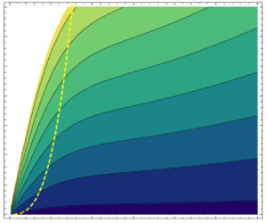
Figure 4. (a) Ratio of skewness and steepness varying with bandwidth in strongly non-Gaussian ($\mu _{4} \approx 0.4$) North Sea data (Stansell Reference Stansell2004), with polynomial fit $\mathfrak{B}(\nu ) \approx 1- \nu \sqrt {2} + 3.5 \nu ^{2}$ at $2 \leq k_{p}h \leq {\rm \pi}$. (b) Contour plot of the same ratio as computed from (4.2) for the fitted function $\mathfrak{B}(\nu, k_{p}h)$ in (a).

with notation $\tilde {\chi }_{i}$ from Mendes et al. (Reference Mendes, Scotti, Brunetti and Kasparian2022)

(4.3a,b)\begin{equation} \tilde{\chi}_{0} = \frac{ \left[ 4 \left( 1 + \dfrac{2k_{p}h}{\sinh{(2k_{p}h)}} \right) - 2 \right] }{ \left( 1 + \dfrac{2k_{p}h}{\sinh{(2k_{p}h)}} \right)^{2} \tanh{k_{p}h} - 4 k_{p}h };\quad \frac{\sqrt{\tilde{\chi}_{1}}}{2} = \frac{3 - \tanh^{2}{(k_{p}h)} }{ 2\tanh^{3}{(k_{p}h)} }. \end{equation}

Although Tayfun and Alkhalidi's model provides a good fit of $\mu _{3}/\varepsilon$ for $k_{p}h > 3$, the sum $\tilde {\chi }_{0} + \sqrt {\tilde {\chi }_{1}} / 2$ stays close to unity for $k_{p}h \geq 2$. Hence, the larger values of the ratio $\mu _{3}/\varepsilon$ for shallower water ($2 \leq k_{p}h \leq {\rm \pi}$) must stem from a dependence of $\mathfrak{B}(\nu )$ on depth. We therefore seek a generalization of (4.2) whereby we fit a function $\mathfrak{B}(\nu, k_{p}h) = 1- \nu \sqrt {2} + f_{k_{p}h} \boldsymbol{\cdot} \nu ^{2}$ capable of providing a smooth transition from $f_{k_{p}h \sim 3} \approx 3.5$ in shallower depths (see figure 4a) to the deep water value $f_{k_{p}h = \infty } \sim 1$ (see (4.1)). Hence, implementing this fit into (2.6) and (2.7) the vertical asymmetry accounting for depth-induced effects is of the type

(4.4)\begin{equation} \mathfrak{S}(\alpha = 2) \approx \frac{ (2+6\varepsilon_{{\ast}}) (7+3\varepsilon_{{\ast}}) }{ 6 (2+3\varepsilon_{{\ast}}) }, \end{equation}

where $\varepsilon _{\ast }$ is the effective steepness

(4.5)\begin{equation} \varepsilon_{{\ast}} \approx \frac{{\rm \pi} \varepsilon}{3\sqrt{2}}[1- \nu \sqrt{2} + f_{k_{p}h} \boldsymbol{\cdot} \nu^{2}] \left(\tilde{\chi}_{0} + \frac{\sqrt{\tilde{\chi}_{1}}}{2} \right). \end{equation}

Figure 4(b) provides a contour plot for the ratio $\mu _{3}/\varepsilon$ taking into account the fitted model of $f_{k_{p}h}$. Here, $f_{k_{p}h}$ is a function of depth that can be obtained through the constraint $\mathfrak{S} \leq 2$ of (2.5) applied to (4.4)

(4.6)\begin{equation} \lim_{\substack{k_{p}h \rightarrow 0 }} \mathfrak{S}(\alpha = 2) \approx \lim_{\substack{k_{p}h \rightarrow 0 } } \frac{ (2+6\varepsilon_{{\ast}}) (7+3\varepsilon_{{\ast}}) }{ 6 (2+3\varepsilon_{{\ast}}) } \leq 2, \end{equation}

thus leading to

(4.7)\begin{equation} 9\varepsilon_{{\ast}}^{2} + 6 \varepsilon_{{\ast}} - 5 \leq 0 \quad \therefore \quad \varepsilon_{{\ast}} \leq \frac{\sqrt{6}-1}{3}. \end{equation}

The function $\mathfrak{B}(\nu, k_{p}h)$ makes the exceedance probability of rogue waves weakly dependent on the bandwidth $\nu$ (Longuet-Higgins Reference Longuet-Higgins1975). Very broad-banded seas ($\nu \geq 1$) are very rare. For example, they account for only 3 % of observed stormy states in the North Sea (Mendes et al. Reference Mendes, Scotti and Stansell2021). These extreme sea conditions are typically short lived and found for instance in hurricanes. Albeit bandwidths much larger than $\nu = 1$ can increase the vertical asymmetry by approximately 5 %–10 %, their lifespan impacts the weighted average of the exceedance probability of rogue waves over a daily forecast by only ${\sim }10\,\%$ because $\nu \sim 0.5$ over 97 % of all 30 min records. Accordingly, we may set $\nu = 1$ as the realistic and effective maximum bandwidth to be considered for estimating the rogue wave exceedance probability. Hence, in the second-order limit we obtain

(4.8)\begin{equation} \lim_{k_{p}h \rightarrow 1/2} \frac{{\rm \pi} \varepsilon}{3\sqrt{2}} f_{k_{p}h} \left(\tilde{\chi}_{0} + \frac{\sqrt{\tilde{\chi}_{1}}}{2} \right) < \frac{\sqrt{6}-1}{3}. \end{equation}

Consequently, broad-banded waves will not exceed the following depth correction:

(4.9)\begin{equation} f_{k_{p}h} (\nu = 1) \lesssim \frac{18\sqrt{2}}{\rm \pi} \approx 8. \end{equation}

Broad-banded waves have an effective steepness of the order of $\varepsilon f_{k_{p}h} \nu ^{2}$. Since finite-depth effects involve the ratio $\varepsilon / k_{p}h$ which it is directly related to $H_{s}/h$ and $f_{k_{p}h}$ grows quickly from deep to intermediate waters (see figure 4a), we expect $f_{k_{p}h}$ to be inversely proportional to the relative depth $k_{p}h$. In order to fulfil (4.6)–(4.9), a sigmoid function provides a good fit with continuous derivative for the North Sea data (see figure 5a)

(4.10)\begin{equation} f_{k_{p}h} \approx \frac{8}{1+7 \tanh^{2}{( k_{p}h/7)}},\quad \nu \leq 1. \end{equation}

Plugging (4.10) into (4.4) introduces an approximation for the vertical asymmetry covering the entire range of second-order theory for narrow and broad-banded irregular waves. In fact, figure 5(b) shows that the vertical asymmetry is almost constant for typical values of mean steepness ($\varepsilon \ll 1/10$) in intermediate and deep waters ($k_{p}h \geq {\rm \pi}/10$). Conversely, sharp increases in the mean steepness will induce a few per cent increase in the vertical asymmetry in the same regimes ($k_{p}h \geq {\rm \pi}/10$). The contour plot in figure 6(b) provides a full description of the variations in asymmetry with depth and steepness. Furthermore, figure 6(a) shows that, in shallow depths, the vertical asymmetry strongly depends on $k_{p}h$ while in deep water it tends to saturate. Figure 6(c) also illustrates the role of bandwidth in increasing the asymmetry, albeit sharp changes are restricted to sufficiently broad spectra ($\nu > 0.8$). Thus, the analysis of field data from the North Sea shows that, as long as the steepness in intermediate water ($k_{p}h > {\rm \pi}/10$) is small ($\varepsilon < 1/10$) or the spectrum narrow $(\nu < 1/2)$, the vertical asymmetry stays close to $\mathfrak{S}= 1.2$. We find this approximation for the vertical asymmetry to be still applicable to the experiments in Trulsen et al. (Reference Trulsen, Raustøl, Jorde and Rye2020) with steeper slope, as shown in Appendix B.

Figure 5. (a) Finite-depth functions $f_{k_{p}h}$ vs data (circles) from figure 4(a). (b) Vertical asymmetry of broad-banded rogue waves $(\nu = 0.5)$ as a function of water depth for different steepness, with the dotted line depicting the empirical mean value $\mathfrak{S} = 1.2$ from Mendes et al. (Reference Mendes, Scotti and Stansell2021, Reference Mendes, Scotti, Brunetti and Kasparian2022). Dashed vertical line marks the limit of validity of second-order theory.

Figure 6. Vertical asymmetry of large and rogue waves as a function of water depth for different mean steepness, bandwidth and normalized height. The dashed line in (b) represents the Ursell limit for second-order theory.

Moreover, the special case of narrow-banded ($\nu = 0$) linear waves ($\varepsilon \ll 1/10$) in deep water leads to $\varepsilon _{\ast } \rightarrow 0$, thus reaching the lower bound of the asymmetry $\mathfrak{S} = 7/6$ for rogue waves. This suggests that, in intermediate waters, narrowing the bandwidth from $\nu = 0.3$ to $\nu = 0$ will have little impact on the amplification of rogue wave statistics due to the negligible change in vertical asymmetry, whereas in shallow water increasing the bandwidth above $\nu = 0.5$ will significantly boost rogue wave occurrence. From the point of view of the theory in Mendes et al. (Reference Mendes, Scotti, Brunetti and Kasparian2022), the asymmetry approximation of (4.4), (4.10) explains why narrow-banded models (Li et al. Reference Li, Draycott, Zheng, Lin, Adcock and Van Den Bremer2021a) are successful in predicting rogue wave statistics travelling past a step in a broad-banded irregular wave background in intermediate water. Provided there is no wave breaking $(H_{s}/h \ll 1)$, the bandwidth effect will play a role in amplifying statistics in shallower depths because of the contributuin of the term $f_{k_{p}h}\nu ^{2}$, as experimentally demonstrated in Doeleman (Reference Doeleman2021).

5. Upper bound for kurtosis atop a shoal

The excess kurtosis has been used in the past two decades as a proxy for how rough nonlinear seas increase the occurrence and intensity of rogue waves. Therefore, in this section we extend our results of § 3 to estimate the maximum kurtosis atop any shoal in the ocean (Janssen & Bidlot Reference Janssen and Bidlot2009; Janssen Reference Janssen2017). The assessment of maximum expected waves over a specific return time at a fixed location is crucial for naval design. Typically, ocean structures and vessels must be designed to sustain expected maximum extreme waves over their lifespan (Borgman Reference Borgman1973; Muir & El-Shaarawi Reference Muir and El-Shaarawi1986). In order to do so, we shall evaluate maxima for the parameters $\mathfrak{S}$ and $\varGamma$. Equations (4.4) and (4.10) provide the upper bound for the vertical asymmetry of rogue waves in the limit of wave breaking: $\mathfrak{S}_{\infty }(k_{p}h = \infty ) \approx 1.387$ in deep water and $\mathfrak{S}_{\infty }(k_{p}h = 0) \approx 1.668$ in shallow water. Since the $\varGamma$ correction is also limited by wave breaking, one finds the bound $\varGamma _{\infty } - 1 \lesssim 1/12$ due to (3.17) of Mendes et al. (Reference Mendes, Scotti, Brunetti and Kasparian2022). Hence, we may approximate

(5.1)\begin{equation} 1 - \frac{1}{\mathfrak{S}^{2}_{\infty} \varGamma_{\infty}} \lesssim 8 (\varGamma_{\infty} - 1). \end{equation}

Approaching the value $\varGamma _{\infty }$ atop the shoal (region III of figure 1), the contribution of the skewness to the amplification of wave statistics near the breaking regime increases such that the relationship between kurtosis and skewness leading to (3.2) is modified and now empirically reduces to $\mu _{4} \approx \mu _{3}^{2}$ (Ma et al. Reference Ma, Ma and Dong2015). Plugging this relationship into (3.1) and comparing it with (2.4) and (5.1), we obtain

(5.2)\begin{equation} \exp({16\alpha^{2} (\varGamma_{\infty} - 1)})\geq 1 + \alpha^{2} (\alpha^{2} - 1) \mu_{4}. \end{equation}

At $\alpha = 2$, the evaluation of the excess kurtosis lies at the region of stability of the Gram–Charlier series and we are able to compute the upper bound for the excess kurtosis in the case of pre-shoal Gaussian statistics (see figure 7)

(5.3)\begin{equation} \mu_{4, \infty} \approx \tfrac{1}{12} [ \exp({64 (\varGamma_{\infty} - 1)}) - 1 ], \end{equation}

where $\varGamma _{\infty }$ varies with water depth. According to (5.3), typical seas with steep and highly asymmetrical broad-banded waves lead to an upper bound for the excess kurtosis of the order of $\mu _{4, \infty } \sim 4$ in intermediate water, see figure 7. We already described that the maximum value of $\varGamma$ is located around $k_{p}h \approx 0.5$ in Mendes et al. (Reference Mendes, Scotti, Brunetti and Kasparian2022) and (3.3) has been validated in figure 2. Therefore, the peak in excess kurtosis will also be located in this region. Experiments conducted in Zhang et al. (Reference Zhang, Ma, Tan, Dong and Benoit2023) found the peak in excess kurtosis in the same region $k_{p}h \approx 0.5$.

Figure 7. Upper bound on kurtosis from (5.3) for $\nu =0.5$ and different pre-shoal mean (significant) steepness $\varepsilon _{0} = H_{s,0}/\lambda _{0}$ subject to linear shoaling. The dashed curve represents the kurtosis in figure 2(a), representative of run 1 of Trulsen et al. (Reference Trulsen, Raustøl, Jorde and Rye2020) and with the bathymetry of figure 1.