


1. Introduction
The dynamics of multiphase systems involving rigid particles suspended in rheologically complex matrices is of considerable interest both from a fundamental perspective and in practical applications, particularly within the field of microfluidics (Van Dinther et al. Reference van Dinther, Schroën, Vergeldt, van der Sman and Boom2012; Shaqfeh Reference Shaqfeh2019). Understanding the hydrodynamic interactions among particles is essential for predicting and controlling their distribution within a suspension, which is critical for optimising processes in many fields, including material science, biotechnology and the pharmaceutical industry.
It is well known that rigid spheres suspended in Newtonian fluids under creeping flow conditions do not exhibit cross-flow migration due to the linearity of the Stokes equations that mathematically describe the system (Happel & Brenner (Reference Happel and Brenner1983)). However, introducing nonlinearity, either through inertia (Ho & Leal (Reference Ho and Leal1974)), complex rheology of the suspending fluid, such as viscoelasticity (D’Avino et al. Reference D’Avino, Greco and Maffettone2017), or particle deformability (Villone & Maffettone Reference Villone and Maffettone2019), enables particle migration. Numerous studies have investigated the motion and migration of rigid particles in non-Newtonian fluids (see, e.g. Lu et al. Reference Lu, Liu, Hu and Xuan2017). The combined lateral and axial motions of particles in pressure-driven flow of non-Newtonian liquids can be harnessed to induce ordered structures (Del Giudice et al. Reference Del Giudice, D’Avino, Greco, Maffettone and Shen2018; Liu et al. Reference Liu, Xu, Xiu, Xiang and Ni2020), whose formation is influenced by factors such as the flow rate and rheological properties of the suspending medium (Del Giudice et al. Reference Del Giudice, D’Avino, Greco, Maffettone and Shen2018) and the geometry of the domain (Jeyasountharan et al. Reference Jeyasountharan, D’Avino and Del Giudice2022). Notably, viscoelastic liquids promote particle repulsion, leading to the formation of uniformly spaced trains of both rigid (D’Avino et al. 2013) and deformable (Esposito et al. Reference Esposito, D’Avino and Villone2024a ) particles. Motivated by the works cited above, this study aims to explore particle interactions in a different rheological context, i.e. yield-stress fluids. These materials exhibit a transition from solid-like to liquid-like behaviour when subjected to a stress that exceeds a critical (yield) value. The physical mechanism underlying this transition is associated with the microstructure of the material, often comprising a network of interacting constituents that maintain a solid-like state under static conditions (Bonn et al. Reference Bonn, Denn, Berthier, Divoux and Manneville2017), but, once a critical stress state is exceeded, the material ‘yields’ and starts to flow.
The dual nature of yield-stress fluids has significant potential for applications such as particle trapping and controlled release (Chaparian & Tammisola (Reference Chaparian and Tammisola2020)). In recent experiments, yield-stress materials have been employed for particle sorting in microfluidic devices, leveraging the combination of solid-like behaviour at rest and fluidity under applied stress to selectively transport or trap particles based on size or applied force (Ovarlez et al. Reference Ovarlez, Mahaut, Deboeuf, Lenoir, Hormozi and Chateau2015). The dynamics of particles in yield-stress fluids has important implications also in various industrial processes, including drilling, cement slurry flows and food manufacturing. The ability to control particle motion in yield-stress materials is crucial for ensuring uniformity, preventing clogging and optimising product consistency (Ruan et al. Reference Ruan, Wu, Bürger, Betancourt, Wang, Wang, Jiao and Wang2021). Previous studies have revealed some key mechanisms that govern particle migration, interaction and suspension stability. For instance, the velocity and stress fields around particles in yield-stress fluids are significantly influenced by the presence of unyielded regions, which resist flow until the applied stress surpasses the yield-stress threshold (Putz et al. Reference Putz, Burghelea, Frigaard and Martinez2008; Fraggedakis et al. Reference Fraggedakis, Dimakopoulos and Tsamopoulos2016). The size of unyielded regions, along with the capacity of particles to deform the surrounding material, plays a critical role in determining particle motion and interactions. Recently, Chaparian & Tammisola (Reference Chaparian and Tammisola2020) demonstrated that, depending on flow conditions and material properties, rigid particles can either experience intermittent flow or become completely arrested in yield-stress fluids. In this study, the authors have shown that the stability of individual particles in Poiseuille flow of a yield-stress fluid depends strongly on their position relative to the yield surface (Chaparian & Tammisola Reference Chaparian and Tammisola2020). Particles may either migrate within the yielded regions or remain trapped in the unyielded plug if the yield stress is sufficiently high. Compared with sedimentation in a quiescent yield-stress fluid, the presence of shear stress in Poiseuille flow destabilises particles at lower buoyancy. Neutrally buoyant particles remain stable only if they are fully contained within the unyielded plug, but the plug can locally expand to accommodate them. These findings suggest that both elasticity and the local stress distribution play crucial roles in particle transport and structuring in yield-stress suspensions. Additionally, recent experiments revealed that even slight fluid elasticity significantly impacts the flow around interacting particles in yield-stress fluids, highlighting the need to better describe the rheological response of these materials through a coupling between elastic and plastic behaviours (Firouznia et al. Reference Firouznia, Metzger, Ovarlez and Hormozi2018).
Incorporating elasticity into yield-stress materials adds further complexity to their flow behaviour. In elastoviscoplastic (EVP) fluids, the interplay among elastic, viscous and plastic effects results in an intricate dynamics, wherein both elastic deformations and yielding significantly influence particle motion. Recent numerical (Fraggedakis et al. Reference Fraggedakis, Dimakopoulos and Tsamopoulos2016; Moschopoulos et al. Reference Moschopoulos, Spyridakis, Varchanis, Dimakopoulos and Tsamopoulos2021; Esposito et al. Reference Esposito, Dimakopoulos and Tsamopoulos2024b ; Kordalis et al. Reference Kordalis, Dimakopoulos and Tsamopoulos2024) and experimental studies (Holenberg et al. Reference Holenberg, Lavrenteva, Shavit and Nir2012; Lopez et al. Reference Lopez, Naccache and de Souza Mendes2018) have highlighted the need to take elastic effects into account in the modelling of yield-stress materials to accurately capture distinct phenomena, e.g. the formation of a negative wake (i.e. flow reversal) behind a rigid sphere settling in moderately concentrated Carbopol solutions, which ‘pure’ viscoplastic models (that neglect elasticity) fail to predict.
In this work, we perform numerical simulations to study the hydrodynamic interactions between two rigid spheres suspended on the axis of a cylindrical tube filled with a yield-stress fluid exhibiting elastic effects, namely, an EVP fluid, subjected to pressure-driven flow. Section 2 is devoted to the description of the problem and the numerical method adopted to solve it, with a validation of our code. In § 3, we present and discuss the results of the study, investigating the role of plasticity, elasticity and confinement through an extensive parametric analysis. Finally, in § 4, we summarise our findings and discuss ideas for future work.
2. Mathematical model
2.1. Governing equations
The geometry of the computational domain is illustrated in figure 1: two non-Brownian rigid spherical particles, both having diameter $D_{\textit{p}}$
, are placed on the axis of a cylindrical tube with diameter
$D_{\textit{p}}$
, are placed on the axis of a cylindrical tube with diameter $D_{\textit{c}}$
filled with an EVP fluid undergoing pressure-driven flow. The initial distance between the surfaces of the particles is
$D_{\textit{c}}$
filled with an EVP fluid undergoing pressure-driven flow. The initial distance between the surfaces of the particles is $d_0$
. The assumption that particles are located along the axis of the tube is supported by previous studies demonstrating that the elasticity of the suspending fluid promotes lateral migration toward the centre of cylindrical channels (D’Avino et al. Reference D’Avino, Greco and Maffettone2017). Furthermore, a numerical study on the role of the yield stress on the migration of a single particle in channel flow of EVP fluids (Chaparian et al. Reference Chaparian, Ardekani, Brandt and Tammisola2020) has indicated that, when inertial forces are not dominant, also the plasticity of the carrier fluid facilitates particle migration toward the centre. This arises from particle rotation, which induces localised yielding within the plug region.
$d_0$
. The assumption that particles are located along the axis of the tube is supported by previous studies demonstrating that the elasticity of the suspending fluid promotes lateral migration toward the centre of cylindrical channels (D’Avino et al. Reference D’Avino, Greco and Maffettone2017). Furthermore, a numerical study on the role of the yield stress on the migration of a single particle in channel flow of EVP fluids (Chaparian et al. Reference Chaparian, Ardekani, Brandt and Tammisola2020) has indicated that, when inertial forces are not dominant, also the plasticity of the carrier fluid facilitates particle migration toward the centre. This arises from particle rotation, which induces localised yielding within the plug region.
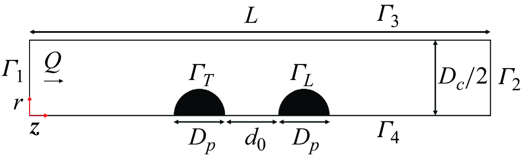
Figure 1. Schematic representation of the system investigated in this work: two rigid spherical particles with diameter $D_{{p}}$
, whose surfaces are initially separated by a distance
$D_{{p}}$
, whose surfaces are initially separated by a distance $d_0$
, are placed on the axis of symmetry of a tube with diameter
$d_0$
, are placed on the axis of symmetry of a tube with diameter $D_{{c}}$
filled with an EVP fluid under pressure-driven flow, with flow rate
$D_{{c}}$
filled with an EVP fluid under pressure-driven flow, with flow rate $Q$
, in the positive
$Q$
, in the positive $z$
direction (from left to right).
$z$
direction (from left to right).
Consequently, we assume that the particles underwent hydrodynamic focusing in a sufficiently long portion of the channel upstream that of our interest here. This allows us to exploit the axial symmetry of the system and reduce the computational domain from three to two dimensions.
The suspending liquid is considered incompressible. In typical microfluidic applications, where highly viscous fluids and small-scale devices are common, the effects of inertia and gravity are negligible, thus we do not include such forces in the mathematical description of the problem. Therefore, the dynamics of the fluid is governed by the mass and momentum balance equations in the following formulation:
 \begin{align} \nabla \cdot \boldsymbol{u}=0, \end{align}
 \begin{align} \nabla \cdot \boldsymbol{T}=\boldsymbol{0}, \end{align}
where $\boldsymbol{u}$
is the velocity vector and
$\boldsymbol{u}$
is the velocity vector and $\boldsymbol{T}$
is the total stress tensor, which can be decomposed as
$\boldsymbol{T}$
is the total stress tensor, which can be decomposed as
 \begin{eqnarray} \boldsymbol{T}=-p\boldsymbol{I}+2\eta _{\mathit{s}}\boldsymbol{D}+\boldsymbol{\tau }, \end{eqnarray}
with $p$
the pressure,
$p$
the pressure, $\boldsymbol{I}$
the identity tensor,
$\boldsymbol{I}$
the identity tensor, $\eta _{\mathit{s}}$
the Newtonian solvent contribution to the viscosity of the fluid,
$\eta _{\mathit{s}}$
the Newtonian solvent contribution to the viscosity of the fluid, $\boldsymbol{D}=(\nabla \boldsymbol{u}+(\nabla \boldsymbol{u})^{\mathrm{T}})/2$
the rate-of-deformation tensor and
$\boldsymbol{D}=(\nabla \boldsymbol{u}+(\nabla \boldsymbol{u})^{\mathrm{T}})/2$
the rate-of-deformation tensor and $\boldsymbol{\tau }$
the extra stress due to the polymeric nature of the EVP fluid. The rheological behaviour of the latter is modelled by a Giesekus-like modification of the Saramito constitutive equation, predicting shear thinning, bounded extensional viscosity and yield stress (Saramito Reference Saramito2007). This reads as
$\boldsymbol{\tau }$
the extra stress due to the polymeric nature of the EVP fluid. The rheological behaviour of the latter is modelled by a Giesekus-like modification of the Saramito constitutive equation, predicting shear thinning, bounded extensional viscosity and yield stress (Saramito Reference Saramito2007). This reads as
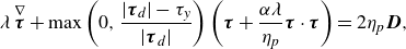 \begin{equation} \lambda \stackrel {\nabla }{\boldsymbol{\tau }}+\max \left (0,\frac {|\boldsymbol{\tau }_{\textit{d}}|-\tau _{\textit{y}}}{|\boldsymbol{\tau }_{\textit{d}}|}\right )\left (\boldsymbol{\tau }+\frac {\alpha \lambda }{\eta _{\mathit{p}}}\boldsymbol{\tau }\cdot \boldsymbol{\tau }\right )=2\eta _{\mathit{p}}\boldsymbol{D}, \end{equation}
where $|\boldsymbol{\tau }_{\textit{d}}|=\sqrt {(\boldsymbol{\tau }_{\textit{d}}:\boldsymbol{\tau }_{\textit{d}})/2}$
is the second invariant of the deviatoric part of the extra stress tensor, in turn defined as
$|\boldsymbol{\tau }_{\textit{d}}|=\sqrt {(\boldsymbol{\tau }_{\textit{d}}:\boldsymbol{\tau }_{\textit{d}})/2}$
is the second invariant of the deviatoric part of the extra stress tensor, in turn defined as
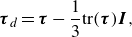 \begin{equation} \boldsymbol{\tau }_{\textit{d}}=\boldsymbol{\tau }-\frac {1}{3}\text{tr}(\boldsymbol{\tau })\boldsymbol{I}, \end{equation}
with ‘tr’ the trace operator. In (2.4), the operator ‘max’ embeds the comparison between $|\boldsymbol{\tau }_{\textit{d}}|$
and the yield stress of the material
$|\boldsymbol{\tau }_{\textit{d}}|$
and the yield stress of the material $\tau _{\textit{y}}$
, incorporating the von Mises criterion (Hill Reference Hill1998), whereas
$\tau _{\textit{y}}$
, incorporating the von Mises criterion (Hill Reference Hill1998), whereas $\lambda$
indicates the relaxation time,
$\lambda$
indicates the relaxation time, $\eta _{\textit{p}}$
is the polymeric contribution to the viscosity and
$\eta _{\textit{p}}$
is the polymeric contribution to the viscosity and $\alpha$
is the ‘mobility’ parameter, which modulates the shear-thinning behaviour of the material. According to (2.4), the yield surface, i.e. the envelope denoting the transition from a viscoelastic solid to a viscoelastic liquid behaviour, is obtained where
$\alpha$
is the ‘mobility’ parameter, which modulates the shear-thinning behaviour of the material. According to (2.4), the yield surface, i.e. the envelope denoting the transition from a viscoelastic solid to a viscoelastic liquid behaviour, is obtained where $|\boldsymbol{\tau }_{\textit{d}}|=\tau _{\textit{y}}$
. The symbol
$|\boldsymbol{\tau }_{\textit{d}}|=\tau _{\textit{y}}$
. The symbol $(^{\nabla })$
denotes the upper-convected time derivative, defined as
$(^{\nabla })$
denotes the upper-convected time derivative, defined as
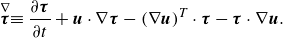 \begin{equation} \stackrel {\nabla }{\boldsymbol{\tau }}\equiv \frac {\partial \boldsymbol{\tau }}{\partial t}+\boldsymbol{u}\cdot \nabla \boldsymbol{\tau }-(\nabla \boldsymbol{u})^{T}\cdot \boldsymbol{\tau }-\boldsymbol{\tau }\cdot \nabla \boldsymbol{u}. \end{equation}
To close the problem, we impose the following boundary conditions:
 \begin{align} &\qquad \boldsymbol{u}=(0,0,U_{{L,T}}) \text{ on } \Gamma _{{L,T}}, \end{align}
 \begin{align} &\qquad\qquad \boldsymbol{u}=\boldsymbol{0} \text{ on } \Gamma _3, \end{align}
 \begin{align} &(\boldsymbol{T}\cdot \boldsymbol{n})|_{\Gamma _1}=-(\boldsymbol{T}\cdot \boldsymbol{n})|_{\Gamma _2}-\Delta p\boldsymbol{n}, \end{align}
 \begin{align} &\qquad \boldsymbol{u}|_{\Gamma _1}=\boldsymbol{u}|_{\Gamma _2}, \end{align}
 \begin{align} & Q=-\int _{\Gamma _{1}}\boldsymbol{u}\cdot \boldsymbol{n}\,{\rm d}S, \end{align}
 \begin{align} &\,\, (\boldsymbol{n}\cdot \boldsymbol{T}\cdot \boldsymbol{t})|_{\Gamma _4}=0, \end{align}
 \begin{align} &\quad (\boldsymbol{n}\cdot \boldsymbol{u})|_{\Gamma _4}=0. \end{align}
Equation (2.7) expresses the no-slip/no-penetration and rigid-body motion conditions on the surfaces of the particles $\Gamma _{\textit{L}}$
and
$\Gamma _{\textit{L}}$
and $\Gamma _{\textit{T}}$
, where the subscripts ‘L’ and ‘T’ stand for ‘leading’ and ‘trailing’, respectively, and
$\Gamma _{\textit{T}}$
, where the subscripts ‘L’ and ‘T’ stand for ‘leading’ and ‘trailing’, respectively, and $U_{\textit{T}}$
and
$U_{\textit{T}}$
and $U_{\textit{L}}$
are the axial components of the translational velocities of the particles (to be computed). On the tube wall
$U_{\textit{L}}$
are the axial components of the translational velocities of the particles (to be computed). On the tube wall $\Gamma _3$
, we impose the no-slip/no-penetration condition through (2.8). The periodicity of velocity and stress between the inflow and outflow boundaries
$\Gamma _3$
, we impose the no-slip/no-penetration condition through (2.8). The periodicity of velocity and stress between the inflow and outflow boundaries $\Gamma _1$
and
$\Gamma _1$
and $\Gamma _2$
is applied through (2.9)–(2.10), where
$\Gamma _2$
is applied through (2.9)–(2.10), where $\Delta p$
indicates the pressure drop between those boundaries (to be computed). A fixed flow rate
$\Delta p$
indicates the pressure drop between those boundaries (to be computed). A fixed flow rate $Q$
is imposed at the inlet section, see (2.11). Finally, axial symmetry conditions are imposed on
$Q$
is imposed at the inlet section, see (2.11). Finally, axial symmetry conditions are imposed on $\Gamma _4$
, see (2.12) and (2.13). In the equations expressing the boundary conditions,
$\Gamma _4$
, see (2.12) and (2.13). In the equations expressing the boundary conditions, $\boldsymbol{n}$
identifies the unit vector normal to the boundary pointing toward the liquid phase, whereas
$\boldsymbol{n}$
identifies the unit vector normal to the boundary pointing toward the liquid phase, whereas $\boldsymbol{t}$
is the unit vector tangential to the boundary. Because of the absence of inertial terms, no initial condition is needed on the velocity field, but an appropriate initial condition is required on the extra stress tensor
$\boldsymbol{t}$
is the unit vector tangential to the boundary. Because of the absence of inertial terms, no initial condition is needed on the velocity field, but an appropriate initial condition is required on the extra stress tensor $\boldsymbol{\tau }$
. We assume the EVP fluid is initially stress free, namely,
$\boldsymbol{\tau }$
. We assume the EVP fluid is initially stress free, namely,
 \begin{equation} \boldsymbol{\tau }|_{t=0}=\boldsymbol{0}. \end{equation}
The hydrodynamic force acting on each particle is specified under the assumption of absence of inertia and external forces. Furthermore, the radial and angular components of such force are identically zero due to the symmetry of the system. Accordingly, the $z$
-component of the total force acting on each spherical surface must be zero, i.e.
$z$
-component of the total force acting on each spherical surface must be zero, i.e.
 \begin{eqnarray} F_{{L,T}}=\int _{\Gamma _{{L,T}}}(\boldsymbol{T}\cdot \boldsymbol{n})\cdot \boldsymbol{e}_{\textit{z}}\,{\rm d}S=0, \end{eqnarray}
with $\boldsymbol{e}_{\textit{z}}$
the unit vector pointing in the
$\boldsymbol{e}_{\textit{z}}$
the unit vector pointing in the $z$
-direction. To obtain the positions of the particles at each time step, we integrate the kinematic equations
$z$
-direction. To obtain the positions of the particles at each time step, we integrate the kinematic equations
 \begin{eqnarray} \frac {{\rm d}z_{{L,T}}}{{\rm d}t}=U_{{L,T}}, \end{eqnarray}
where $z_{\textit{L}}$
and
$z_{\textit{L}}$
and $z_{\textit{T}}$
identify the axial positions of the centres of the particles. The initial conditions associated with (2.16) are imposed by specifying the initial positions of the particles
$z_{\textit{T}}$
identify the axial positions of the centres of the particles. The initial conditions associated with (2.16) are imposed by specifying the initial positions of the particles $z_{{L,T}}|_{t=0}=z_{{L,T}}^0$
.
$z_{{L,T}}|_{t=0}=z_{{L,T}}^0$
.
2.2. Dimensionless equations
To make the mathematical model of the system dimensionless, we choose the diameter of the cylindrical tube $D_{\textit{c}}$
as the characteristic length, the average inlet velocity of the continuous phase
$D_{\textit{c}}$
as the characteristic length, the average inlet velocity of the continuous phase $\bar U = 4Q/(\pi D_{\textit{c}}^2)$
as the characteristic velocity and
$\bar U = 4Q/(\pi D_{\textit{c}}^2)$
as the characteristic velocity and $\eta _0 \bar U/D_{\textit{c}}$
, with
$\eta _0 \bar U/D_{\textit{c}}$
, with $\eta _0=\eta _{\textit{s}}+\eta _{\textit{p}}$
the zero-shear viscosity, as the characteristic stress (viscous scaling). Hence, the balance equations can be rewritten in dimensionless form as
$\eta _0=\eta _{\textit{s}}+\eta _{\textit{p}}$
the zero-shear viscosity, as the characteristic stress (viscous scaling). Hence, the balance equations can be rewritten in dimensionless form as
 \begin{align} &\qquad\qquad\quad \nabla ^{*}\cdot \boldsymbol{u}^{*}=0, \end{align}
 \begin{align} &-\nabla ^{*}p^{*}+\eta _{\mathit{r}}\nabla ^{*2} \boldsymbol{u}^{*}+\nabla ^{*}\cdot \boldsymbol{\tau }^{*}=\boldsymbol{0}, \end{align}
where the asterisks denote dimensionless quantities. The dimensionless constitutive equation of the EVP fluid is
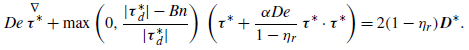 \begin{equation} \textit{De}\stackrel {\nabla }{\boldsymbol{\tau }^{*}}+\max \left (0,\frac {|\boldsymbol{\tau }^*_{\textit{d}}|-\textit{Bn}}{|\boldsymbol{\tau }^*_{\textit{d}}|}\right ) \left (\boldsymbol{\tau }^{*}+\frac {\alpha \textit{De}}{1-\eta _{\textit{r}}}\,\boldsymbol{\tau }^{*}\cdot \boldsymbol{\tau }^{*}\right )=2(1-\eta _{\mathit{r}})\boldsymbol{D}^{*} .\end{equation}
In the equations reported above, three dimensionless parameters appear, namely, the Deborah number, the Bingham number and the viscosity ratio, defined as follows:
 \begin{align} &\,\, \textit{De}=\frac {4 \lambda Q}{\pi D_{\textit{c}}^3}, \end{align}
 \begin{align} & \textit{Bn}=\frac {\pi \tau _{\textit{y}}D_{\textit{c}}^3}{4 \eta _{0} Q}, \end{align}
 \begin{align} &\quad \eta _{\mathit{r}}=\frac {\eta _{\mathit{s}}}{\eta _0}. \end{align}
The Deborah number measures the ratio between the characteristic times of the fluid and of the flow, the Bingham number measures the ratio between the yield stress (plasticity) and the viscous stress in the fluid and, finally, the viscosity ratio measures the relevance of the solvent contribution to the total viscosity of the material. In addition, two other dimensionless quantities play a role in the problem, i.e. the mobility parameter $\alpha$
and the confinement ratio
$\alpha$
and the confinement ratio $\beta =D_{\textit{p}}/D_{\textit{c}}$
.
$\beta =D_{\textit{p}}/D_{\textit{c}}$
.
In this work, we fix $\eta _{\textit{r}}=0.1$
. The dynamics of the particle pair is studied as De, Bn,
$\eta _{\textit{r}}=0.1$
. The dynamics of the particle pair is studied as De, Bn, $\beta$
and
$\beta$
and $\alpha$
are varied in realistic ranges that might be attained in experiments. All the results reported below are dimensionless; for brevity, the asterisks are omitted.
$\alpha$
are varied in realistic ranges that might be attained in experiments. All the results reported below are dimensionless; for brevity, the asterisks are omitted.
2.3. Numerical method, convergence and validation
We solve the equations governing the system by means of a mixed finite-element method, incorporating the discrete elastic viscous stress splitting stabilisation technique (Guénette & Fortin Reference Guénette and Fortin1995; Bogaerds et al. Reference Bogaerds, Grillet, Peters and Baaijens2002; Kynch & Phillips Reference Kynch and Phillips2017) and the streamline–upwind/Petrov Galerkin technique to stabilise the convective term in the constitutive equation (Brooks & Hughes (Reference Brooks and Hughes1982)). A continuous quadratic interpolation for the velocity and a continuous linear interpolation for the pressure, the stress tensor and the auxiliary velocity gradient are used to satisfy the Ladyzhenskaya–Babuška–Brezzi condition (Boffi et al. Reference Boffi, Brezzi and Fortin2013). To enhance convergence at high Deborah number, we utilise the log-conformation formulation (Fattal & Kupferman Reference Fattal and Kupferman2004). The rigid-body motion is enforced through constraints applied at each node on the surfaces of the particles by using Lagrange multipliers. The arbitrary Lagrangian–Eulerian method is employed to accommodate the motion of the mesh nodes around the particles (Hu et al. Reference Hu, Patankar and Zhu2001).The continuity and momentum balance equations are decoupled from the constitutive equation. In this formulation, the time-discretised constitutive equation is substituted into the momentum balance equation in order to obtain a linear Stokes-like system. The constitutive equation is discretised by a second-order semi-implicit Gear scheme. At each time step, after the assembly of the finite-element matrices, the two resulting linear non-symmetric sparse systems are solved employing the parallel direct solver PARDISO (Schenk & Gärtner Reference Schenk and Gärtner2004). To mitigate mesh distortion resulting from particle motion, we rigidly translate the mesh in the flow direction with a velocity equal to the average velocity of the two particles. This ensures that any remaining mesh distortion is primarily due to the gradual variation of the distance between the particles.

Figure 2. Example of a typical mesh used in the simulations. The region around the particles is displayed.
We discretise the computational domain with an unstructured mesh made of quadratic triangular elements, an example of which is displayed in figure 2. Furthermore, to ensure that our calculations are accurate even when the particles get close, we impose that a minimum number of mesh elements must be present between the surfaces of the particles, where larger gradients of velocity and stresses are expected. Preliminary tests show that 5–6 elements in the gap are sufficient to obtain grid-independent results even in the hardest case, i.e. when the particles are separated by a minimal distance $d_{0} = 0.05$
. When the interparticle distance increases, the number of elements in the gap is increased accordingly to maintain an adequate distribution of the computational nodes. The effect of the grid size is explored through a mesh independence analysis.
$d_{0} = 0.05$
. When the interparticle distance increases, the number of elements in the gap is increased accordingly to maintain an adequate distribution of the computational nodes. The effect of the grid size is explored through a mesh independence analysis.
The results of an example case are reported in figure 3. In panel (a), we vary the number of elements on the boundaries of the particles $N$
and track the evolution of the most relevant kinematic quantity, the particle relative velocity
$N$
and track the evolution of the most relevant kinematic quantity, the particle relative velocity $\Delta U = U_{\textit{L}} - U_{\textit{T}}$
, as a function of time, the values of the parameters being given in the caption. From the superposition of the curves, we deduce that even a mesh having 30 elements on the boundaries of the particles would be adequate, but, for ‘safety’, we employ meshes with
$\Delta U = U_{\textit{L}} - U_{\textit{T}}$
, as a function of time, the values of the parameters being given in the caption. From the superposition of the curves, we deduce that even a mesh having 30 elements on the boundaries of the particles would be adequate, but, for ‘safety’, we employ meshes with $N$
= 45 in our simulations, except in critical cases having a very short inter-particle distance, where finer meshes having
$N$
= 45 in our simulations, except in critical cases having a very short inter-particle distance, where finer meshes having $N$
= 60 are used. In panel (b), further tests are carried out on another very sensitive quantity, the second invariant of the deviatoric part of the extra stress tensor,
$N$
= 60 are used. In panel (b), further tests are carried out on another very sensitive quantity, the second invariant of the deviatoric part of the extra stress tensor, $|\boldsymbol{\tau }_{\textit{d}}|$
, whose values are tracked along the axis of symmetry at
$|\boldsymbol{\tau }_{\textit{d}}|$
, whose values are tracked along the axis of symmetry at $t = 60$
for the three different meshes. Panel (c) presents the temporal evolution of the percentage error in the relative velocity between the particles for different mesh resolutions, specifically
$t = 60$
for the three different meshes. Panel (c) presents the temporal evolution of the percentage error in the relative velocity between the particles for different mesh resolutions, specifically $ N = 30$
(M1),
$ N = 30$
(M1), $ N = 45$
(M2) and
$ N = 45$
(M2) and $ N = 60$
(M3). The distributions of yielded/unyielded regions corresponding to the three meshes are displayed in panels (d) to (f). Again, the fair agreement of the data suggests that a mesh having
$ N = 60$
(M3). The distributions of yielded/unyielded regions corresponding to the three meshes are displayed in panels (d) to (f). Again, the fair agreement of the data suggests that a mesh having $N = 45$
is adequate for our calculations.
$N = 45$
is adequate for our calculations.
Finally, due to the periodic boundary conditions applied on the inlet and outlet sections of the channel, we verify that the length of the computational domain $L$
is sufficiently large to avoid any interaction between the particles and their periodic images along the flow direction. A channel length
$L$
is sufficiently large to avoid any interaction between the particles and their periodic images along the flow direction. A channel length $L = 100 D_{\textit{p}}$
is found to be adequate and used in all the calculations presented in this work. The whole set of simulations has been performed on blades with two hexacore processors Intel Xeon E5649@2.53 GHz and 48 Gb of RAM, requiring computational times between 2 and 4 days depending on the values of the parameters, the cases at De = 2.0 and Bn = 0.4 being the most demanding.
$L = 100 D_{\textit{p}}$
is found to be adequate and used in all the calculations presented in this work. The whole set of simulations has been performed on blades with two hexacore processors Intel Xeon E5649@2.53 GHz and 48 Gb of RAM, requiring computational times between 2 and 4 days depending on the values of the parameters, the cases at De = 2.0 and Bn = 0.4 being the most demanding.
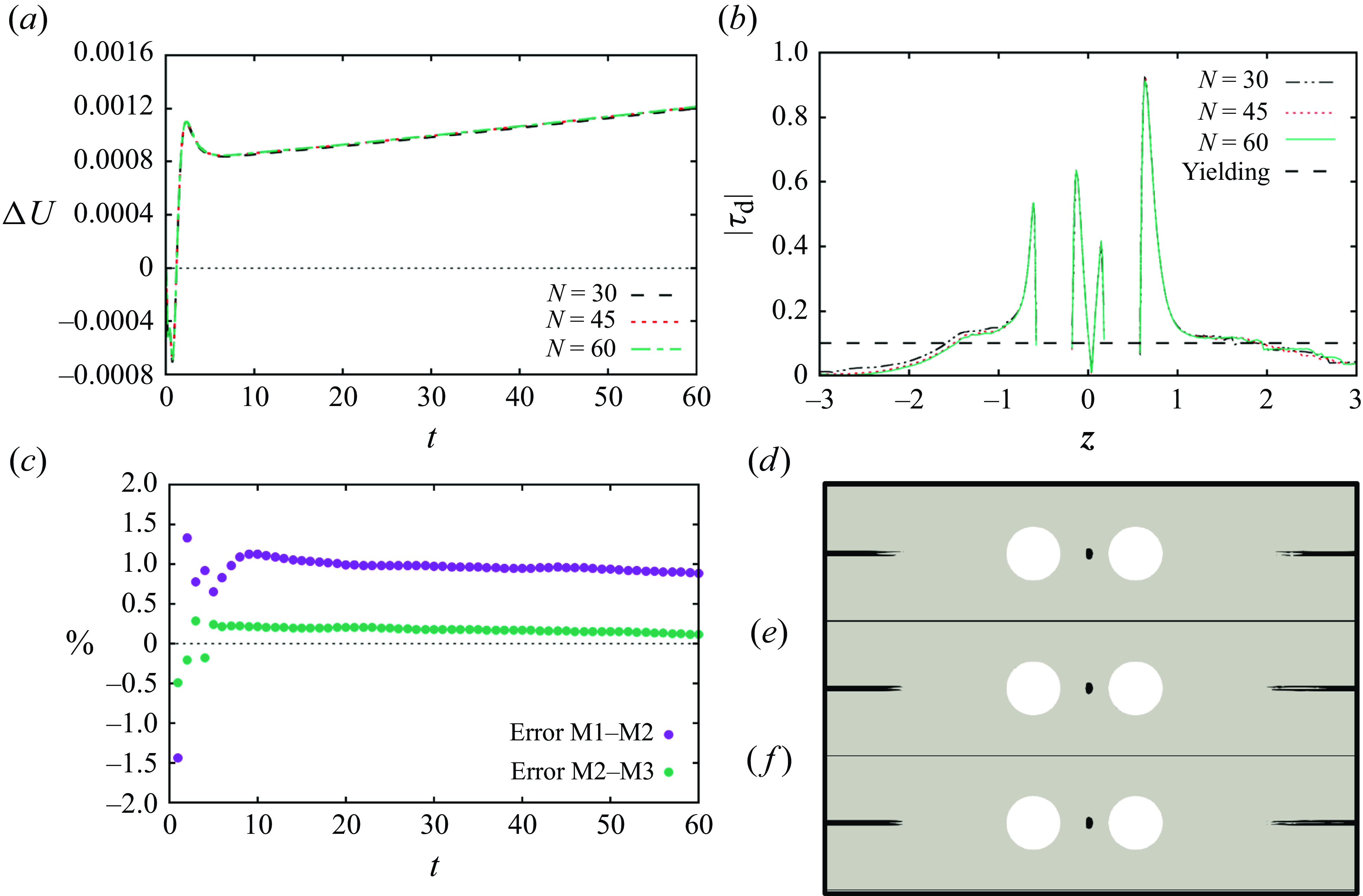
Figure 3. Mesh convergence results. (a) Time evolution of the particle relative velocity $\Delta U=U_{\textit{L}} - U_{\textit{T}}$
and (b) profile of
$\Delta U=U_{\textit{L}} - U_{\textit{T}}$
and (b) profile of $|\boldsymbol{\tau }_{\textit{d}}|$
at
$|\boldsymbol{\tau }_{\textit{d}}|$
at $t = 60$
along the axis of symmetry of the channel (where
$t = 60$
along the axis of symmetry of the channel (where $z=0$
represents the midpoint between the surfaces of the particles) for three meshes characterised by a different number of elements on the boundaries of the particles (
$z=0$
represents the midpoint between the surfaces of the particles) for three meshes characterised by a different number of elements on the boundaries of the particles ( $N$
= 30, 45 and 60, see legend). (c) Time evolution of the percentage error in the relative velocities between
$N$
= 30, 45 and 60, see legend). (c) Time evolution of the percentage error in the relative velocities between $N$
= 30 (M1),
$N$
= 30 (M1), $N$
= 45 (M2) and
$N$
= 45 (M2) and $N$
= 60 (M3). (d)–(f) Yielded (grey) and unyielded (black) regions at
$N$
= 60 (M3). (d)–(f) Yielded (grey) and unyielded (black) regions at $t = 60$
for
$t = 60$
for $N$
= 30, 45 and 60, respectively. The dimensionless parameters are De = 1.0, Bn = 0.1,
$N$
= 30, 45 and 60, respectively. The dimensionless parameters are De = 1.0, Bn = 0.1, $\eta _{\textit{r}}=0.1$
,
$\eta _{\textit{r}}=0.1$
, $\beta =0.4$
,
$\beta =0.4$
, $d_{0} = 0.25$
; the time step is
$d_{0} = 0.25$
; the time step is $\Delta t = 10^{-3}$
.
$\Delta t = 10^{-3}$
.
3. Results
In this section, we present and discuss the results obtained from our simulations. Subsection 3.1 is dedicated to the analysis of the transient dynamics of the system, comparing cases at a given set of values of the dimensionless parameters and different inter-particle initial distances. We find that, beyond an initial start-up due to the development of viscoelastic stresses, the relative velocities of the particles obtained at different initial distances collapse onto a single master curve as a function of the relative distance, similarly to what happens to pairs of rigid particles in viscoelastic liquids (D’Avino et al. Reference D’Avino, Hulsen and Maffettone2013) and pairs of soft particles in both Newtonian and viscoelastic matrices (Villone & Maffettone (Reference Villone and Maffettone2019); Esposito et al. Reference Esposito, D’Avino and Villone2024a ). The analysis of such master curves at different values of the dimensionless parameters is reported in § 3.2, exploring, in particular, the effects of plasticity (i.e. yield stress), elasticity (i.e. relaxation time) and confinement.
3.1. Transient dynamics
To investigate the transient evolution of particle relative velocities and distances, we establish a ‘base case’ with given flow conditions, material properties of the suspending fluid and confinement of the particles. Specifically, we set De = 0.5, Bn = 0.2 and $\beta =0.4$
. These values of the dimensionless parameters can be obtained, for example, in a realistic system where particles with a diameter
$\beta =0.4$
. These values of the dimensionless parameters can be obtained, for example, in a realistic system where particles with a diameter $D_{\textit{p}} = 160\,\mu \mathrm{m}$
are suspended in an EVP fluid characterised by a yield stress
$D_{\textit{p}} = 160\,\mu \mathrm{m}$
are suspended in an EVP fluid characterised by a yield stress $\tau _{\textit{y}} = 1\,\mathrm{Pa}$
, a relaxation time
$\tau _{\textit{y}} = 1\,\mathrm{Pa}$
, a relaxation time $\lambda = 0.25\,\mathrm{s}$
and a zero-shear viscosity
$\lambda = 0.25\,\mathrm{s}$
and a zero-shear viscosity $\eta _{0} = 2.22\,\mathrm{pa}{s}$
, flowing with flow rate
$\eta _{0} = 2.22\,\mathrm{pa}{s}$
, flowing with flow rate $Q = 6\,\mu \mathrm{l\, min^{-1}}$
in a cylindrical channel with diameter
$Q = 6\,\mu \mathrm{l\, min^{-1}}$
in a cylindrical channel with diameter $D_{\textit{c}} = 400\,\mu \mathrm{m}$
. To validate the assumption of inertialess conditions, we calculate the corresponding Reynolds number, defined as
$D_{\textit{c}} = 400\,\mu \mathrm{m}$
. To validate the assumption of inertialess conditions, we calculate the corresponding Reynolds number, defined as $\textit{Re} = 4 \rho Q /(\pi D_{\textit{c}} \eta _0) = 1.4 \times 10^{-4}$
, with
$\textit{Re} = 4 \rho Q /(\pi D_{\textit{c}} \eta _0) = 1.4 \times 10^{-4}$
, with $\rho \sim 10^{3}\rm \,Kg\, m^{-3}$
the fluid density. Since this value is extremely small, the inertial effects are indeed negligible.
$\rho \sim 10^{3}\rm \,Kg\, m^{-3}$
the fluid density. Since this value is extremely small, the inertial effects are indeed negligible.

Figure 4. Transient evolution of the particle relative velocity $\Delta U$
at De = 0.5, Bn = 0.2,
$\Delta U$
at De = 0.5, Bn = 0.2, $\beta =0.4$
and
$\beta =0.4$
and $d_0$
= 0.1, 0.4, 0.9 (see legend). The initial oscillations are caused by the development of viscoelastic stresses around the particles.
$d_0$
= 0.1, 0.4, 0.9 (see legend). The initial oscillations are caused by the development of viscoelastic stresses around the particles.
In figure 4, we report the transient evolution of the particle relative velocity at three different inter-particle initial distances, namely, $d_0$
= 0.1, 0.4 and 0.9. The relative velocity of two particles starting at
$d_0$
= 0.1, 0.4 and 0.9. The relative velocity of two particles starting at $d_0$
= 0.1 is always negative, i.e. they always attract. On the other hand, when the initial inter-particle distance is larger, the relative velocity is positive, thus the particles progressively separate.
$d_0$
= 0.1 is always negative, i.e. they always attract. On the other hand, when the initial inter-particle distance is larger, the relative velocity is positive, thus the particles progressively separate.
To better identify what determines an attractive or a repulsive inter-particle interaction, we analyse the extra stress contribution to the axial component of the force acting on the two particles
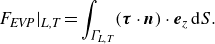 \begin{eqnarray} F_{\textit{EVP}}|_{\textit{L,T}}=\int _{\Gamma _{\textit{L,T}}}(\boldsymbol{\tau }\cdot \boldsymbol{n})\cdot \boldsymbol{e}_{\textit{z}}\,{\rm d}S .\end{eqnarray}
The outward-pointing normal vector to the particle surface can be decomposed as
 \begin{equation} \boldsymbol{n} = \sin (\phi ) \textbf{e}_r + \cos (\phi ) \textbf{e}_z, \end{equation}
where $\phi$
is the polar angle with respect to a reference frame with origin in the particle centre. Hence, (3.1) can be rewritten (in dimensionless form) as
$\phi$
is the polar angle with respect to a reference frame with origin in the particle centre. Hence, (3.1) can be rewritten (in dimensionless form) as
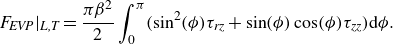 \begin{equation} F_{\textit{EVP}}|_{\textit{L,T}}=\frac {\pi \beta ^2}{2}\int _0^\pi (\sin ^2(\phi )\tau _{\textit{rz}}+\sin (\phi )\cos (\phi )\tau _{\textit{zz}}){\rm d}\phi .\end{equation}
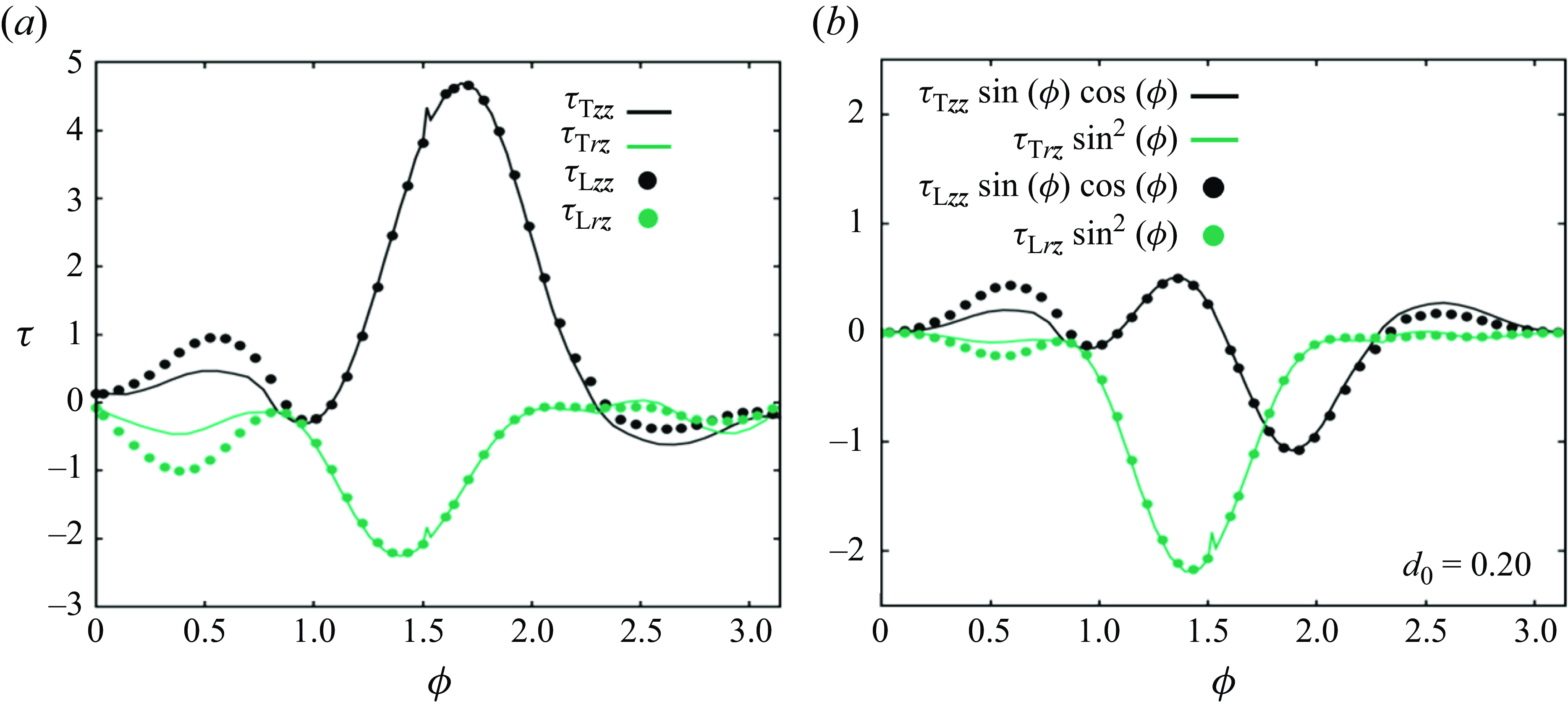
Figure 5. (a) Axial and shear components of the extra stress tensor as a function of the polar angle for the trailing and leading particles for $d_0=0.2$
. (b) The same stress components multiplied by pre-factors as in (3.3). The other parameters are De = 0.5, Bn = 0.2,
$d_0=0.2$
. (b) The same stress components multiplied by pre-factors as in (3.3). The other parameters are De = 0.5, Bn = 0.2, $\beta =0.4$
,
$\beta =0.4$
, $t = 45$
.
$t = 45$
.
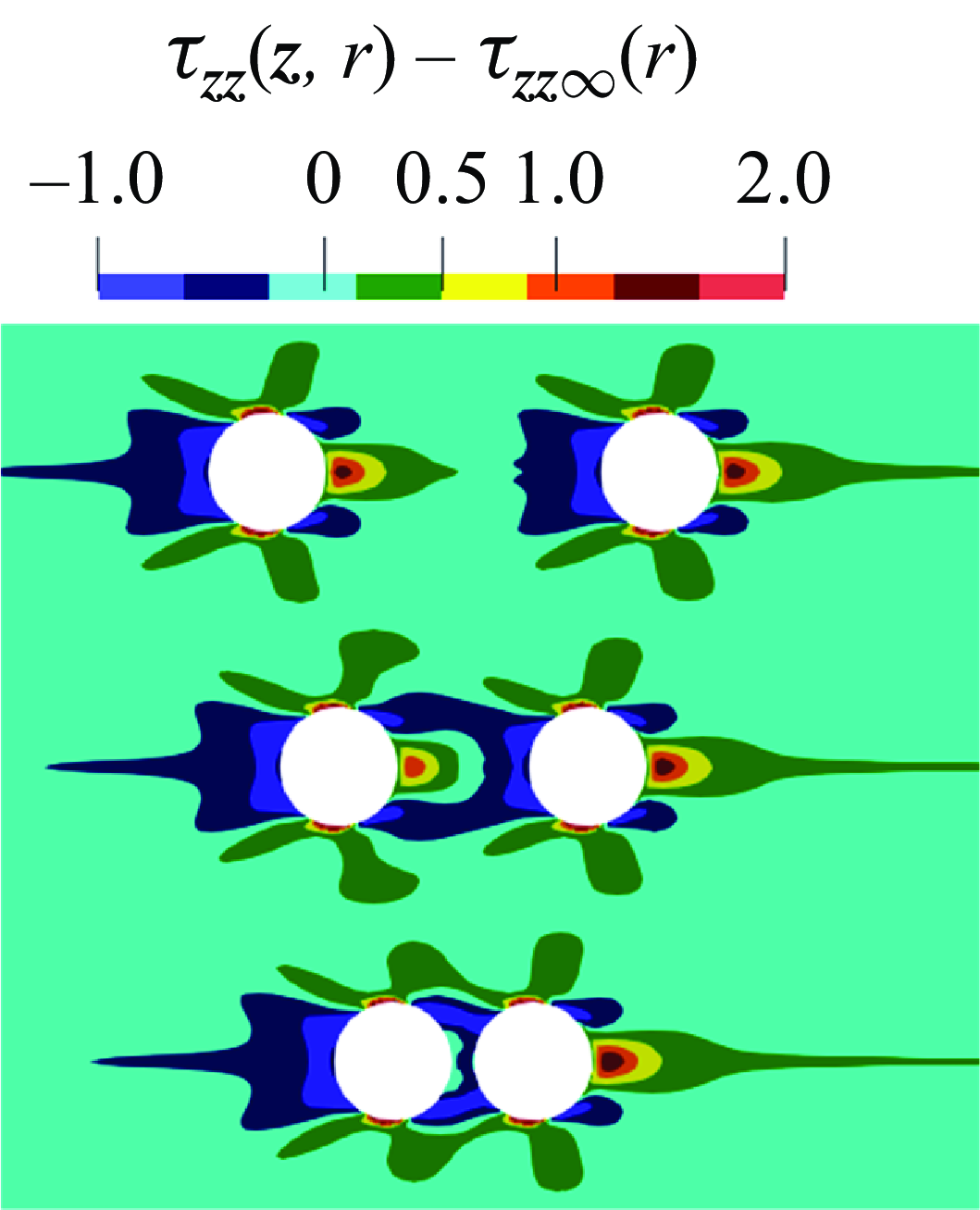
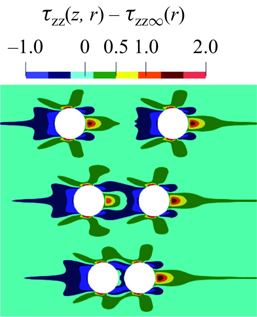
Figure 6. Perturbation of the axial normal extra stress field at De = 0.5, Bn = 0.2, $\beta =0.4$
,
$\beta =0.4$
, $t = 45$
and
$t = 45$
and $d_0$
= 0.9, 0.4, and 0.1 (from top to bottom). The particles move from left to right.
$d_0$
= 0.9, 0.4, and 0.1 (from top to bottom). The particles move from left to right.
Therefore, the hoop stresses do not directly contribute to the EVP force in the $z$
-direction and the only terms are the shear
$z$
-direction and the only terms are the shear $\tau _{\textit{rz}}$
and axial
$\tau _{\textit{rz}}$
and axial $\tau _{{zz}}$
components. Figure 5(a) shows the trends of the axial (black) and shear (green) components of the extra stress tensor as a function of the polar angle for the trailing (lines) and leading (symbols) particles for
$\tau _{{zz}}$
components. Figure 5(a) shows the trends of the axial (black) and shear (green) components of the extra stress tensor as a function of the polar angle for the trailing (lines) and leading (symbols) particles for $d_0=0.2$
. Figure 5(b) reports the same quantities multiplied by the corresponding pre-factors as in (3.3). It turns out that the predominant contribution is the axial one whereas they become comparable when multiplied by the surface normal unit vector. However, the quantitative differences between the stress components acting on the leading and trailing particles are minimal, with nearly identical values observed regardless of the interparticle distance. Similar trends are observed for larger separation distances. This observation suggests that the stress state within the interparticle gap, rather than the direct action of the EVP force on the particle surfaces, primarily dictates the attractive or repulsive nature of the interparticle interaction.
$d_0=0.2$
. Figure 5(b) reports the same quantities multiplied by the corresponding pre-factors as in (3.3). It turns out that the predominant contribution is the axial one whereas they become comparable when multiplied by the surface normal unit vector. However, the quantitative differences between the stress components acting on the leading and trailing particles are minimal, with nearly identical values observed regardless of the interparticle distance. Similar trends are observed for larger separation distances. This observation suggests that the stress state within the interparticle gap, rather than the direct action of the EVP force on the particle surfaces, primarily dictates the attractive or repulsive nature of the interparticle interaction.
We then examine the extra stress field around the particles by plotting in figure 6 the long-time ( $t = 45$
) maps of the particle-caused perturbation of the axial normal component of the extra stress, denoted as
$t = 45$
) maps of the particle-caused perturbation of the axial normal component of the extra stress, denoted as $\tau _{\textit{zz}} (r,z) - \tau _{\textit{zz}\infty } (r)$
, where
$\tau _{\textit{zz}} (r,z) - \tau _{\textit{zz}\infty } (r)$
, where $\tau _{{zz}\infty }$
represents the value of
$\tau _{{zz}\infty }$
represents the value of $\tau _{\textit{zz}}$
in the absence of particles (only depending on
$\tau _{\textit{zz}}$
in the absence of particles (only depending on $r$
). Once the viscoelastic stresses have fully developed, a similar stress field is observed at the back of the trailing particle and at the front of the leading one whatever the initial inter-particle distance: behind the trailing particle, a region where
$r$
). Once the viscoelastic stresses have fully developed, a similar stress field is observed at the back of the trailing particle and at the front of the leading one whatever the initial inter-particle distance: behind the trailing particle, a region where $\tau _{\textit{zz}} - \tau _{{zz}\infty }$
is negative is generated, indicating compressive stresses, whereas an extended region where
$\tau _{\textit{zz}} - \tau _{{zz}\infty }$
is negative is generated, indicating compressive stresses, whereas an extended region where $\tau _{\textit{zz}} - \tau _{{zz}\infty }$
is positive appears in front of the leading particle, denoting tensile stresses. A key qualitative difference emerges in the fluid region in between the particles if we compare the case with the smallest initial distance (
$\tau _{\textit{zz}} - \tau _{{zz}\infty }$
is positive appears in front of the leading particle, denoting tensile stresses. A key qualitative difference emerges in the fluid region in between the particles if we compare the case with the smallest initial distance ( $d_0$
= 0.1, bottom row in figure 6) and those with larger distances (
$d_0$
= 0.1, bottom row in figure 6) and those with larger distances ( $d_0$
= 0.4 and 0.9, top and medium rows in figure 6). At
$d_0$
= 0.4 and 0.9, top and medium rows in figure 6). At $d_0$
= 0.1, the particles are connected through a region where
$d_0$
= 0.1, the particles are connected through a region where $\tau _{\textit{zz}} - \tau _{{zz}\infty }$
is negative; in contrast, at
$\tau _{\textit{zz}} - \tau _{{zz}\infty }$
is negative; in contrast, at $d_0$
= 0.4 and 0.9, the greater distance between the particles allows high tensile stresses to develop in front of the trailing particle, which may potentially push the particles apart. These observations suggest that the distribution of
$d_0$
= 0.4 and 0.9, the greater distance between the particles allows high tensile stresses to develop in front of the trailing particle, which may potentially push the particles apart. These observations suggest that the distribution of $\tau _{\textit{zz}}$
in the gap between the particles may play a crucial role in driving their dynamics. It is also interesting to remark that, as the initial distance between the particles increases from 0.4 to 0.9, the repulsive interaction weakens and the stress fields around the two particles become more similar: it is, of course, expected that, as the distance between the particles increases, the stress distribution around each particle converges to that of an isolated one, with the relative velocity approaching zero.
$\tau _{\textit{zz}}$
in the gap between the particles may play a crucial role in driving their dynamics. It is also interesting to remark that, as the initial distance between the particles increases from 0.4 to 0.9, the repulsive interaction weakens and the stress fields around the two particles become more similar: it is, of course, expected that, as the distance between the particles increases, the stress distribution around each particle converges to that of an isolated one, with the relative velocity approaching zero.
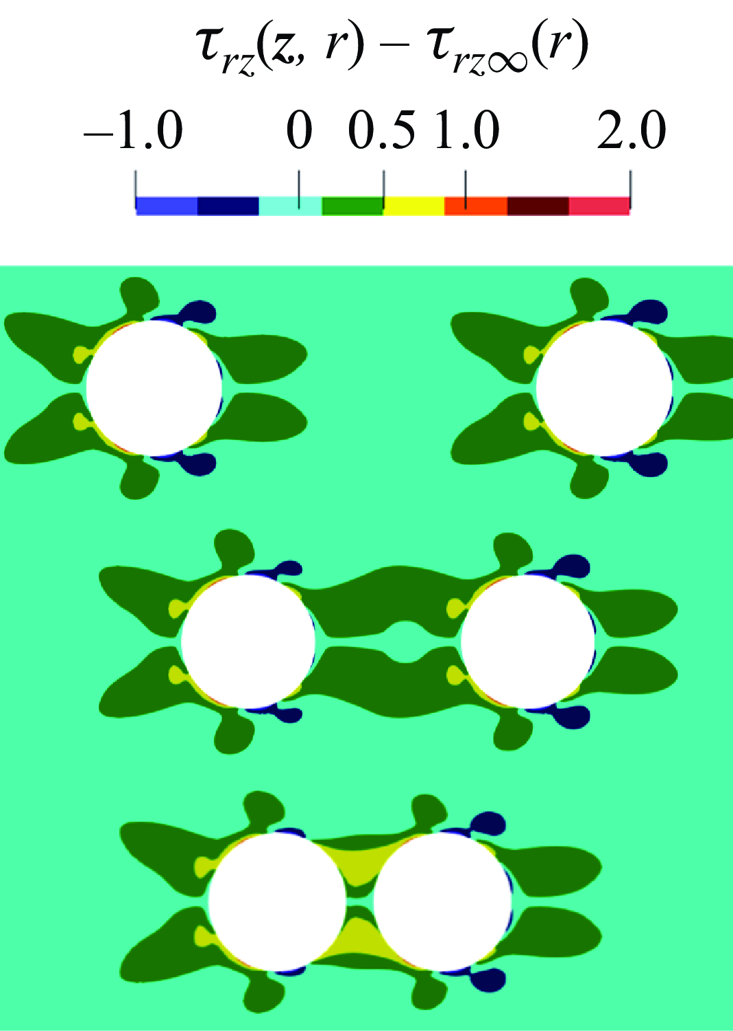
Figure 7. Perturbation of the shear extra stress field at De = 0.5, Bn = 0.2, $\beta =0.4$
,
$\beta =0.4$
, $t = 45$
and
$t = 45$
and $d_0$
= 0.9, 0.4, and 0.1 (from top to bottom). The particles move from left to right.
$d_0$
= 0.9, 0.4, and 0.1 (from top to bottom). The particles move from left to right.
Also the distribution of the perturbed shear stress, $\tau _{\textit{rz}} - \tau _{\textit{rz}\infty }$
, presented in figure 7, offers valuable insights. At small interparticle distances (e.g.
$\tau _{\textit{rz}} - \tau _{\textit{rz}\infty }$
, presented in figure 7, offers valuable insights. At small interparticle distances (e.g. $d_{0}=0.1$
), a shear bridge forms, connecting the front of the trailing particle with the back of the leading one. This shear bridge diminishes in intensity as the interparticle distance increases. The influence of shear bridges on the attractive dynamics has been extensively investigated for two rising bubbles in EVP materials (see Kordalis et al. Reference Kordalis, Pema, Androulakis, Dimakopoulos and Tsamopoulos2023, Reference Kordalis, Dimakopoulos and Tsamopoulos2024).
$d_{0}=0.1$
), a shear bridge forms, connecting the front of the trailing particle with the back of the leading one. This shear bridge diminishes in intensity as the interparticle distance increases. The influence of shear bridges on the attractive dynamics has been extensively investigated for two rising bubbles in EVP materials (see Kordalis et al. Reference Kordalis, Pema, Androulakis, Dimakopoulos and Tsamopoulos2023, Reference Kordalis, Dimakopoulos and Tsamopoulos2024).
From the stress field distributions, it appears that the distinction in the stress state is more pronounced in terms of the axial perturbed normal stress component than in the shear perturbed stress. Furthermore, it is noteworthy that previous simulations employing the exponential Phan–Thien–Tanner (e-PTT) viscoelastic constitutive model have demonstrated a significant suppression of attractive dynamics (De Micco et al. Reference De Micco, D’Avino, Trofa, Villone and Maffettone2024). A key distinction between the Giesekus and e-PTT models lies in their extensional rheological behaviour: at high extension rates, the e-PTT model exhibits extension-rate thinning, whereas the Giesekus model exhibits extension-rate hardening. In contrast, the shear predictions of both models are similar, exhibiting shear-thinning behaviour at higher shear rates. Consequently, it is reasonable to deduce that the extensional behaviour, particularly along the axis of symmetry in the interconnecting space between the particles, is responsible for the observed differences in the dynamics.
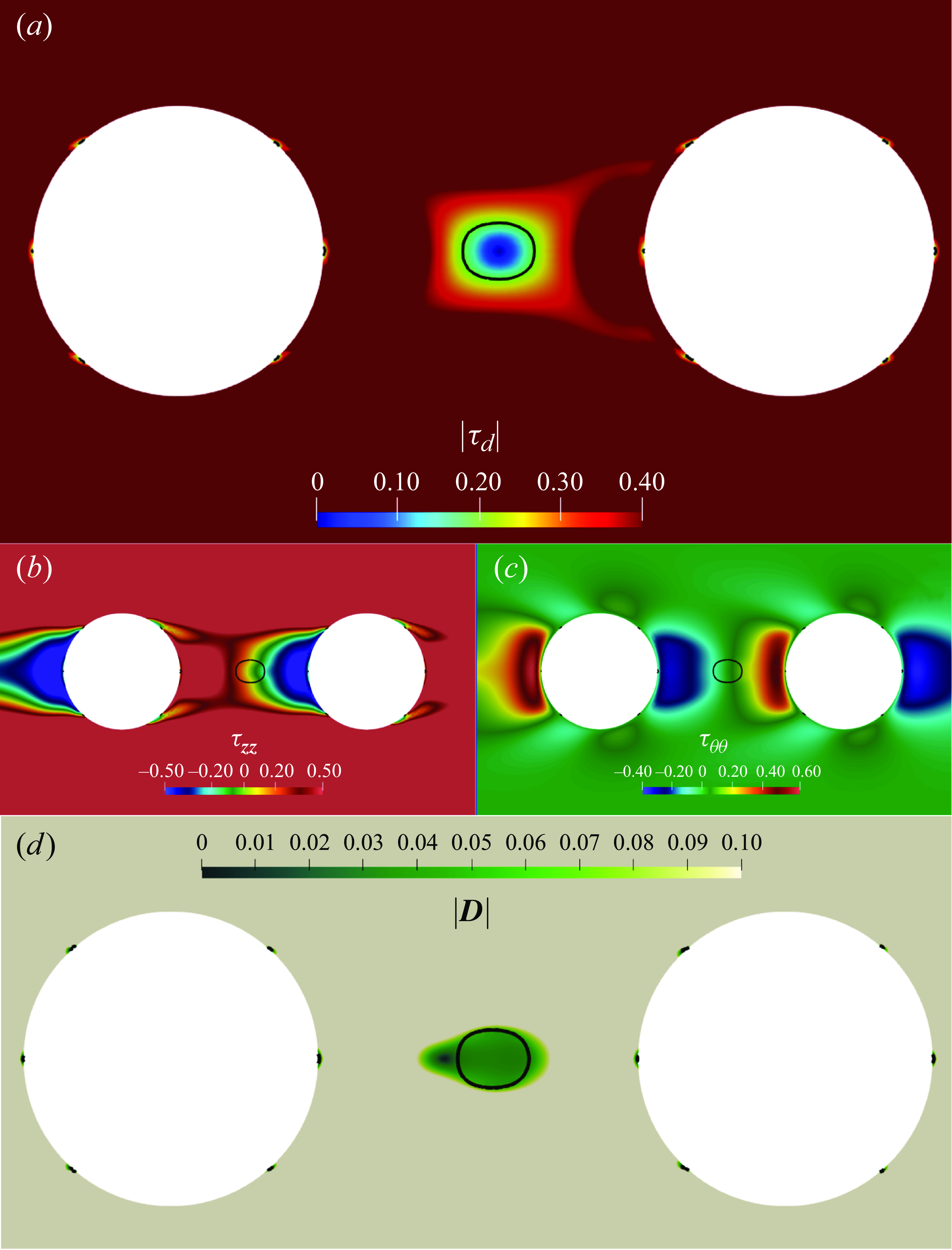
Figure 8. (a) Map of the second invariant of the deviatoric part of the extra stress tensor $|\boldsymbol{\tau }_{\textit{d}}|$
around the particles at De = 0.5, Bn = 0.2,
$|\boldsymbol{\tau }_{\textit{d}}|$
around the particles at De = 0.5, Bn = 0.2, $\beta =0.4$
,
$\beta =0.4$
, $t = 45$
and
$t = 45$
and $d_0$
= 0.4. The yield surface, i.e. the region where
$d_0$
= 0.4. The yield surface, i.e. the region where $|\boldsymbol{\tau }_{\textit{d}}| = \textit{Bn}$
, is indicated with a black continuous line. Distribution of
$|\boldsymbol{\tau }_{\textit{d}}| = \textit{Bn}$
, is indicated with a black continuous line. Distribution of $\tau _{\textit{zz}}$
(b),
$\tau _{\textit{zz}}$
(b), $\tau _{\theta \theta }$
(c) and of the magnitude of the rate-of-deformation tensor
$\tau _{\theta \theta }$
(c) and of the magnitude of the rate-of-deformation tensor $|\boldsymbol{D}|$
(d) around the particles for the same values of the parameters.
$|\boldsymbol{D}|$
(d) around the particles for the same values of the parameters.
Examining the contours of the second invariant of the deviatoric component of the extra stress tensor is crucial for distinguishing yielded regions, where the material behaves as a shear-thinning viscoelastic liquid, from unyielded regions that exhibit a viscoelastic solid behaviour. We recall that the condition that separates the two regimes is $|\boldsymbol{\tau }_{\textit{d}}| = \textit{Bn}$
(with Bn = 0.2, in this case). In figure 8(a), we show the contours of
$|\boldsymbol{\tau }_{\textit{d}}| = \textit{Bn}$
(with Bn = 0.2, in this case). In figure 8(a), we show the contours of $|\boldsymbol{\tau }_{\textit{d}}|$
at
$|\boldsymbol{\tau }_{\textit{d}}|$
at $t = 45$
and
$t = 45$
and $d_0$
= 0.4, identifying the yield surface as a solid black line. Notably, we observe the formation of an unyielded island in between the two particles, whose existence can be understood by inspecting separately the normal components of the extra stress. The axial symmetry condition implies that the components
$d_0$
= 0.4, identifying the yield surface as a solid black line. Notably, we observe the formation of an unyielded island in between the two particles, whose existence can be understood by inspecting separately the normal components of the extra stress. The axial symmetry condition implies that the components $\tau _{\textit{rz}}$
and
$\tau _{\textit{rz}}$
and $\tau _{{rr}}$
are identically zero on the axis of the channel and, consequently, very small around it. On the other hand, the axial and angular normal components of the extra stress,
$\tau _{{rr}}$
are identically zero on the axis of the channel and, consequently, very small around it. On the other hand, the axial and angular normal components of the extra stress, $\tau _{\textit{zz}}$
and
$\tau _{\textit{zz}}$
and $\tau _{\theta \theta }$
, are not negligible and exhibit a sign change while crossing the yield surface. Specifically, the axial stress component
$\tau _{\theta \theta }$
, are not negligible and exhibit a sign change while crossing the yield surface. Specifically, the axial stress component $\tau _{\textit{zz}}$
switches from positive values in front of the trailing particle to negative values behind the leading particle, see figure 8(b), whereas the angular component
$\tau _{\textit{zz}}$
switches from positive values in front of the trailing particle to negative values behind the leading particle, see figure 8(b), whereas the angular component $\tau _{\theta \theta }$
does the opposite, see figure 8(c). The net result is a balance between the two stress components leading to the condition
$\tau _{\theta \theta }$
does the opposite, see figure 8(c). The net result is a balance between the two stress components leading to the condition $|\boldsymbol{\tau }_{\textit{d}}| = \textit{Bn}$
. Furthermore, six small unyielded islands are observed on the surfaces of the spheres, where the material behaves as a viscoelastic solid, showing an almost null rate of deformation, as shown in figure 8(d), where the map of the magnitude of the rate-of-deformation tensor
$|\boldsymbol{\tau }_{\textit{d}}| = \textit{Bn}$
. Furthermore, six small unyielded islands are observed on the surfaces of the spheres, where the material behaves as a viscoelastic solid, showing an almost null rate of deformation, as shown in figure 8(d), where the map of the magnitude of the rate-of-deformation tensor $|\boldsymbol{D}|$
is reported. Indeed, in the proximity of these regions, the components
$|\boldsymbol{D}|$
is reported. Indeed, in the proximity of these regions, the components $\tau _{\textit{zz}}$
and
$\tau _{\textit{zz}}$
and $\tau _{\theta \theta }$
change their sign, while the shear component
$\tau _{\theta \theta }$
change their sign, while the shear component $\tau _{\textit{rz}}$
(not shown) is not sufficiently strong to make the material yield.
$\tau _{\textit{rz}}$
(not shown) is not sufficiently strong to make the material yield.
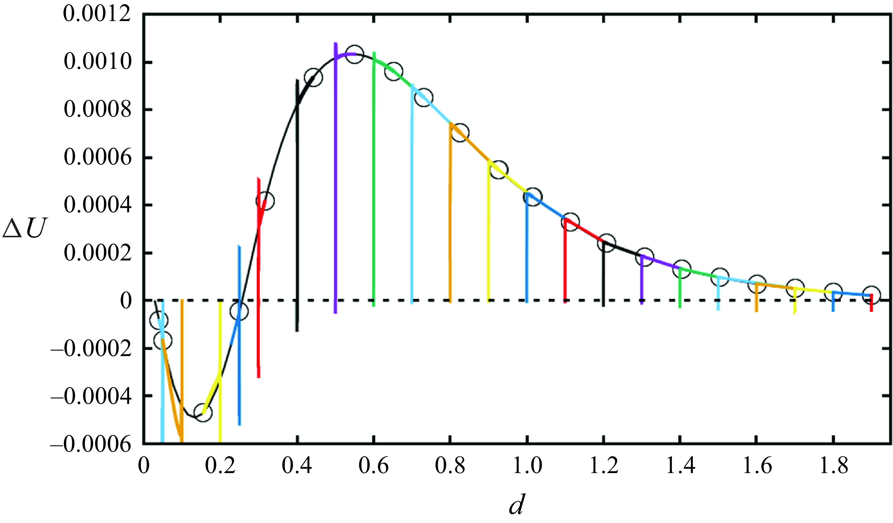
Figure 9. Master curve of the particle relative velocity $\Delta U$
as a function of the inter-particle distance
$\Delta U$
as a function of the inter-particle distance $d$
at De = 0.5, Bn = 0.2 and
$d$
at De = 0.5, Bn = 0.2 and $\beta = 0.4$
. The coloured curves correspond to simulations having different initial distances
$\beta = 0.4$
. The coloured curves correspond to simulations having different initial distances $d_0$
(time is implicit). The empty circles identify data taken at ‘long time’ (i.e. well beyond the initial build-up of viscoelastic stresses) from simulations at different values of
$d_0$
(time is implicit). The empty circles identify data taken at ‘long time’ (i.e. well beyond the initial build-up of viscoelastic stresses) from simulations at different values of $d_0$
. The continuous black line (master curve) is obtained through a polynomial fit of the data.
$d_0$
. The continuous black line (master curve) is obtained through a polynomial fit of the data.
By running simulations at various initial inter-particle distances, we observe that, after the exhaustion of the initial oscillations (like those appearing in figure 4), the long-time dynamics of the particle relative velocity as a function of the inter-particle distance converges onto a single master curve, indicating that, given the confinement and the material and operating parameters, once the viscoelastic stresses have fully developed, the dynamics of the particles is completely determined by their current separation distance. This is illustrated in figure 9, where we report the evolution of the relative velocity as a function of the distance between the particles, showing the superposition of the curves corresponding to different initial distances $d_{0}$
. The dual dynamics (repulsion and attraction) described in figure 4 is clearly visible: there is, indeed, a critical inter-particle distance,
$d_{0}$
. The dual dynamics (repulsion and attraction) described in figure 4 is clearly visible: there is, indeed, a critical inter-particle distance, $d \approx 0.25$
, below which the particles exhibit an attractive behaviour (
$d \approx 0.25$
, below which the particles exhibit an attractive behaviour ( $\Delta U \lt 0$
) and above which they repel each other (
$\Delta U \lt 0$
) and above which they repel each other ( $\Delta U \gt 0$
). This critical distance represents an unstable equilibrium point, where any small perturbation would lead to either attraction or repulsion between the particles. At very large distances,
$\Delta U \gt 0$
). This critical distance represents an unstable equilibrium point, where any small perturbation would lead to either attraction or repulsion between the particles. At very large distances, $d \gtrsim 2$
, the particles behave as if they were isolated, with their relative velocity approaching zero.
$d \gtrsim 2$
, the particles behave as if they were isolated, with their relative velocity approaching zero.
3.2. Effect of the parameters
Let us now explore the effects of the interplay among plasticity, elasticity and confinement on the particle pair dynamics. In figure 10, we display the particle relative velocity master curves at $\beta =0.4$
, two values of De (1.0 on the left and 2.0 on the right) and, for each, four values of Bn (as reported in the legends). Notably, at De = 1.0 (figure 10
a), we observe that, in the ‘purely’ viscoelastic case (Bn = 0), the particles attract at separation distance
$\beta =0.4$
, two values of De (1.0 on the left and 2.0 on the right) and, for each, four values of Bn (as reported in the legends). Notably, at De = 1.0 (figure 10
a), we observe that, in the ‘purely’ viscoelastic case (Bn = 0), the particles attract at separation distance $d \lesssim 0.18$
; conversely, in ‘fully’ EVP cases (
$d \lesssim 0.18$
; conversely, in ‘fully’ EVP cases ( $\textit{Bn} \neq 0$
), the attractive region is replaced by a range of separation distance values characterised by a zero relative velocity, i.e. the particles travel at fixed distance. At De = 2.0 (figure 10
b), the particles always repel at Bn = 0, whereas, at
$\textit{Bn} \neq 0$
), the attractive region is replaced by a range of separation distance values characterised by a zero relative velocity, i.e. the particles travel at fixed distance. At De = 2.0 (figure 10
b), the particles always repel at Bn = 0, whereas, at $\textit{Bn} \gt 0$
, a range of
$\textit{Bn} \gt 0$
, a range of $d$
values characterised by
$d$
values characterised by $\Delta U = 0$
appears again.
$\Delta U = 0$
appears again.
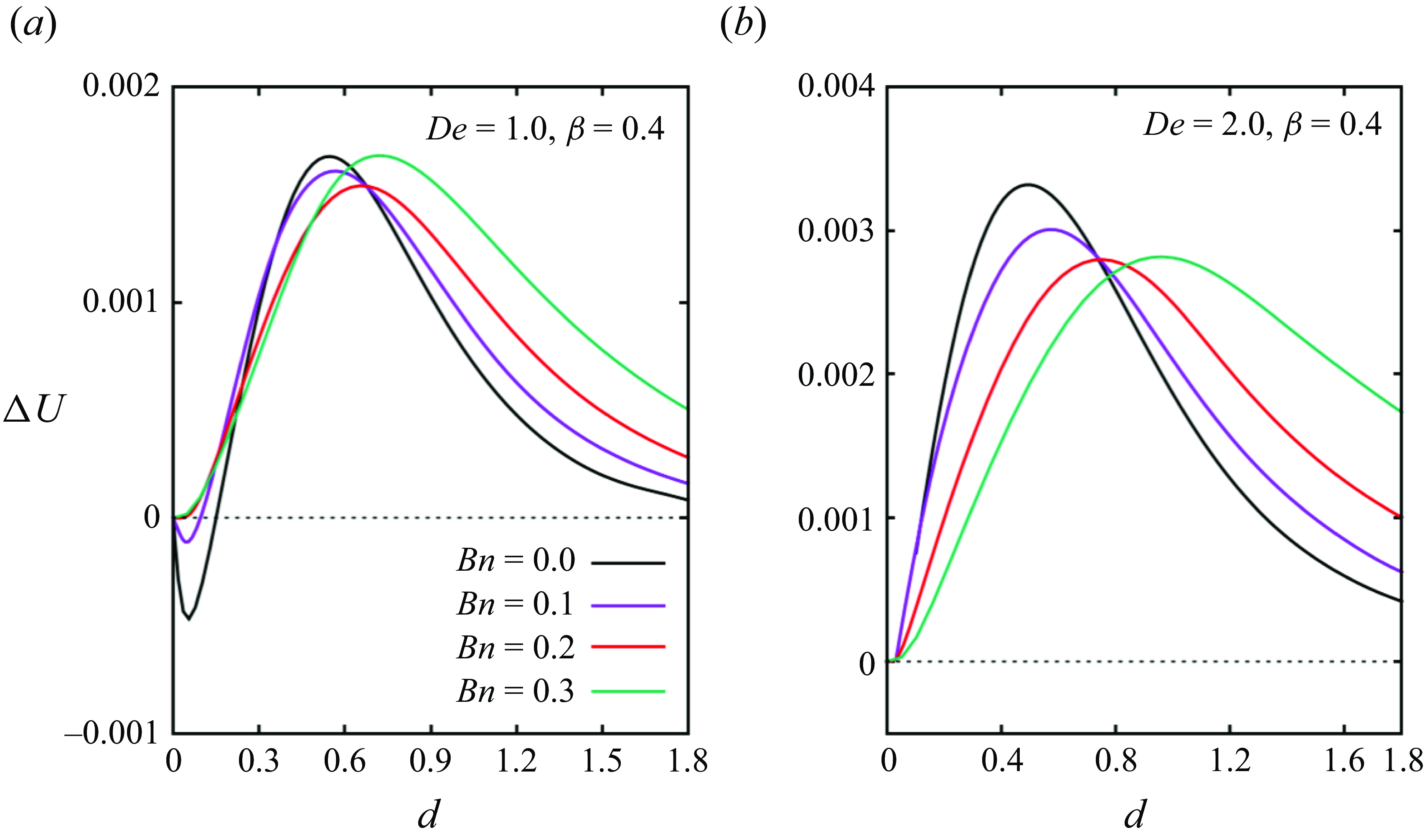
Figure 10. Master curves of the particle relative velocity $\Delta U$
as a function of the inter-particle distance
$\Delta U$
as a function of the inter-particle distance $d$
at
$d$
at $\beta =0.4$
, panel (a)
$\beta =0.4$
, panel (a) $\textit{De} = 1.0$
and panel (b)
$\textit{De} = 1.0$
and panel (b) $\textit{De} = 2.0$
, and different values of Bn (see legends).
$\textit{De} = 2.0$
, and different values of Bn (see legends).
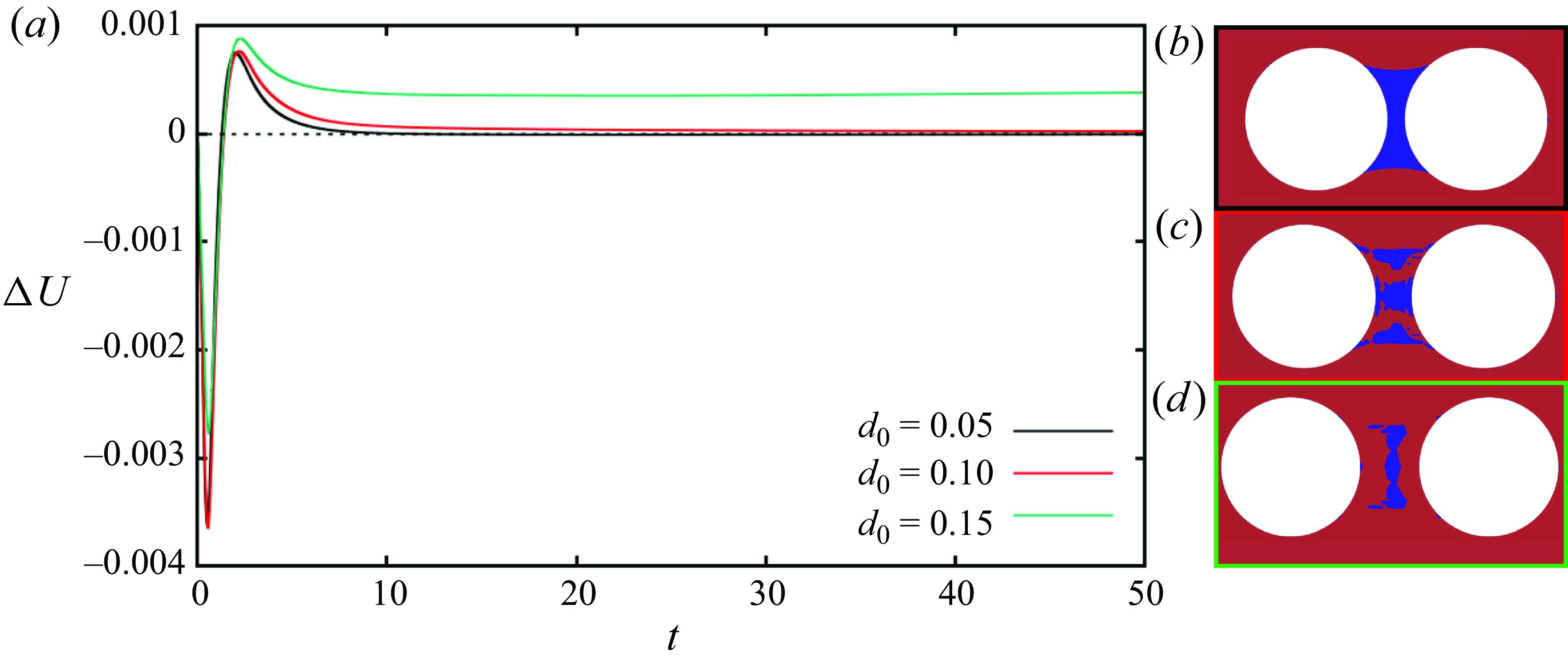
Figure 11. (a) Time evolution of the particle relative velocity $\Delta U$
at De = 1.0, Bn = 0.2,
$\Delta U$
at De = 1.0, Bn = 0.2, $\beta =0.4$
and
$\beta =0.4$
and $d_{0} = 0.05, 0.1, 0.15$
(see legend). On the right, the yielded (red) and unyielded (blue) fluid regions around the particles are shown at
$d_{0} = 0.05, 0.1, 0.15$
(see legend). On the right, the yielded (red) and unyielded (blue) fluid regions around the particles are shown at $t = 40$
and
$t = 40$
and $d_{0} = 0.05$
(b), 0.1 (c) and 0.15 (d).
$d_{0} = 0.05$
(b), 0.1 (c) and 0.15 (d).
To further inspect this scenario, we examine the transient evolution of $\Delta U$
at De = 1.0, Bn = 0.2,
$\Delta U$
at De = 1.0, Bn = 0.2, $\beta =0.4$
and
$\beta =0.4$
and $d_{0} = 0.05, 0.1, 0.15$
, see figure 11. Whatever the initial separation distance, the velocity oscillations induced by the fluid stress build-up persist for approximately 5 time units; after that, a relevant difference is observed: indeed, at
$d_{0} = 0.05, 0.1, 0.15$
, see figure 11. Whatever the initial separation distance, the velocity oscillations induced by the fluid stress build-up persist for approximately 5 time units; after that, a relevant difference is observed: indeed, at $d_{0}$
= 0.05 and 0.1, the relative velocity decays to zero (thus, the separation distance does not change anymore), whereas, at
$d_{0}$
= 0.05 and 0.1, the relative velocity decays to zero (thus, the separation distance does not change anymore), whereas, at $d_{0}$
= 0.15, it tends to a quasi-steady positive value, indicating repulsion. This can be physically explained by looking at the yielded and unyielded regions in the three cases, see figure 11(b–d). At
$d_{0}$
= 0.15, it tends to a quasi-steady positive value, indicating repulsion. This can be physically explained by looking at the yielded and unyielded regions in the three cases, see figure 11(b–d). At $d_{0}$
= 0.05 and 0.1 (panels b and c), the particles are connected by an unyielded region, where the material behaves as a viscoelastic solid: in this zone, the suspending phase undergoes moderate elastic deformation, which forces the particles to stay close to each other, leading to a nearly null relative velocity. In contrast, at
$d_{0}$
= 0.05 and 0.1 (panels b and c), the particles are connected by an unyielded region, where the material behaves as a viscoelastic solid: in this zone, the suspending phase undergoes moderate elastic deformation, which forces the particles to stay close to each other, leading to a nearly null relative velocity. In contrast, at $d_{0} = 0.15$
(panel d), there is still an unyielded region between the particles, yet this is detached from their surfaces, thus allowing them to separate at a finite rate, as shown by the green curve in figure 11(a).
$d_{0} = 0.15$
(panel d), there is still an unyielded region between the particles, yet this is detached from their surfaces, thus allowing them to separate at a finite rate, as shown by the green curve in figure 11(a).
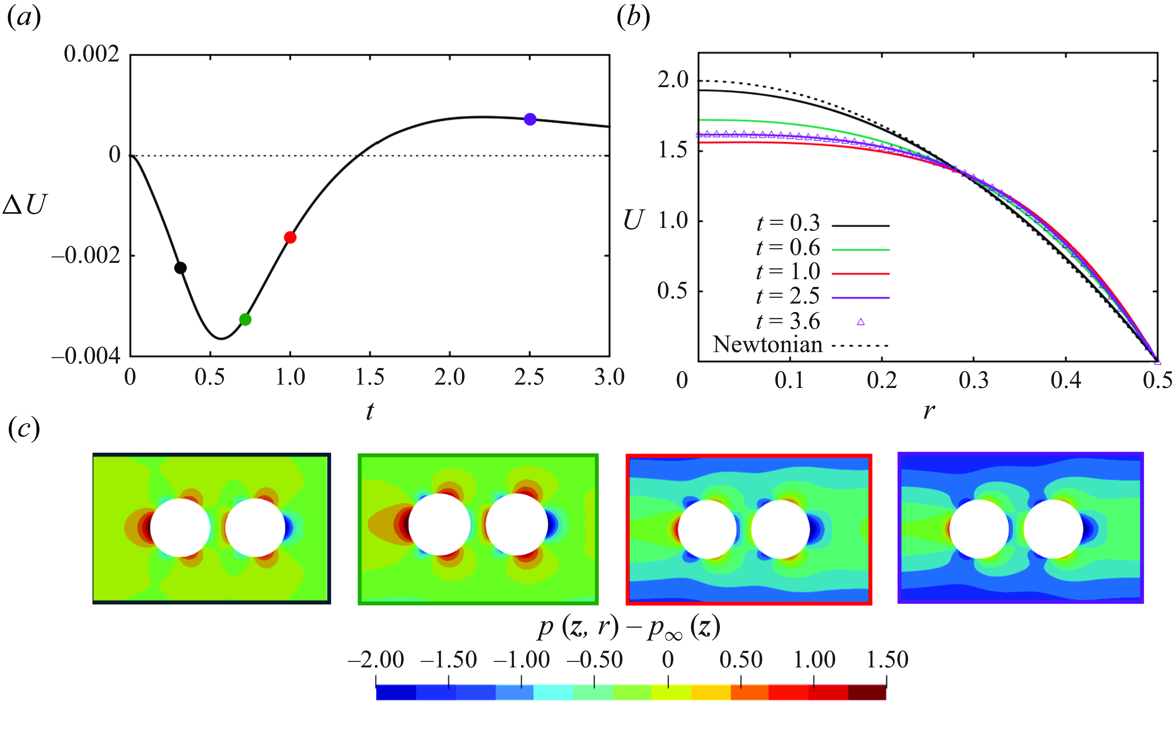
Figure 12. (a) Short-time evolution of the particle relative velocity $\Delta U$
at De = 1.0, Bn = 0.2,
$\Delta U$
at De = 1.0, Bn = 0.2, $\beta =0.4$
and
$\beta =0.4$
and $d_{0} = 0.1$
. (b) Radial profiles of the axial velocity of a pure Saramito–Giesekus fluid during the initial stress build-up at the same values of De and Bn as in panel (a). (c) Perturbation of the pressure field around the particles at the same values of the parameters as in panel (a) and
$d_{0} = 0.1$
. (b) Radial profiles of the axial velocity of a pure Saramito–Giesekus fluid during the initial stress build-up at the same values of De and Bn as in panel (a). (c) Perturbation of the pressure field around the particles at the same values of the parameters as in panel (a) and $t = 0.3, 0.6, 1.0, 2.5$
(from left to right).
$t = 0.3, 0.6, 1.0, 2.5$
(from left to right).
By looking at figure 11, it can be observed that, whatever the final relative velocity of the particles, there is always a negative undershoot at short time. As a consequence, starting from the initial condition where their velocity is null and the fluid is stress free, the particles approach during the initial stages of their dynamics. The time scale of such behaviour is comparable to the relaxation time of the fluid, during which the velocity profile of the suspending phase evolves to its fully developed shape. An explanation for the short-time attraction is illustrated in figure 12, where the case with $d_{0} = 0.10$
is presented. Panel (a) presents a magnified view of the short-time evolution (
$d_{0} = 0.10$
is presented. Panel (a) presents a magnified view of the short-time evolution ( $t \in [0,3]$
) of the particle relative velocity. Here, negative values of
$t \in [0,3]$
) of the particle relative velocity. Here, negative values of $\Delta U$
are observed for
$\Delta U$
are observed for $t \lesssim 1.4$
. Notably, the slope of the curve is negative for
$t \lesssim 1.4$
. Notably, the slope of the curve is negative for $t \lesssim 0.5$
, indicating that the particles are accelerating toward each other in this time span. By looking at the radial profiles of the axial velocity of the material in the absence of particles, in figure 12(b) we see that, for
$t \lesssim 0.5$
, indicating that the particles are accelerating toward each other in this time span. By looking at the radial profiles of the axial velocity of the material in the absence of particles, in figure 12(b) we see that, for $t \lt 1.0$
, the profile progressively flattens in a region around the tube axis: this effect is due to the local shear rate approaching zero where an unyielded island forms, causing the material to behave as a viscoelastic solid; afterwards, the maximum velocity of the fluid increases and the velocity profile reaches its fully developed shape. Correspondingly, particle attraction is replaced by repulsion. In figure 12(c), we display the contours of the perturbed pressure field around the particles, calculated as
$t \lt 1.0$
, the profile progressively flattens in a region around the tube axis: this effect is due to the local shear rate approaching zero where an unyielded island forms, causing the material to behave as a viscoelastic solid; afterwards, the maximum velocity of the fluid increases and the velocity profile reaches its fully developed shape. Correspondingly, particle attraction is replaced by repulsion. In figure 12(c), we display the contours of the perturbed pressure field around the particles, calculated as $p(z,r)-p_\infty (z)$
, where the undisturbed pressure field of the fluid in absence of the spheres is calculated as
$p(z,r)-p_\infty (z)$
, where the undisturbed pressure field of the fluid in absence of the spheres is calculated as $p_\infty (z)=\Delta p - (\Delta p/L)z$
, at four progressively increasing time values, i.e.
$p_\infty (z)=\Delta p - (\Delta p/L)z$
, at four progressively increasing time values, i.e. $t = 0.3, 0.6, 1.0, 2.5$
. In the earlier stages (
$t = 0.3, 0.6, 1.0, 2.5$
. In the earlier stages ( $t = 0.3, 0.6$
), we observe positive values of the pressure perturbation behind the leading particle and negative values in front of the trailing particle, indicating a compression of the fluid in the region in between the particles that makes these approach. Later (
$t = 0.3, 0.6$
), we observe positive values of the pressure perturbation behind the leading particle and negative values in front of the trailing particle, indicating a compression of the fluid in the region in between the particles that makes these approach. Later ( $t = 1.0, 2.5$
), the pressure difference significantly diminishes, with a consequent reduction in particle attraction.
$t = 1.0, 2.5$
), the pressure difference significantly diminishes, with a consequent reduction in particle attraction.
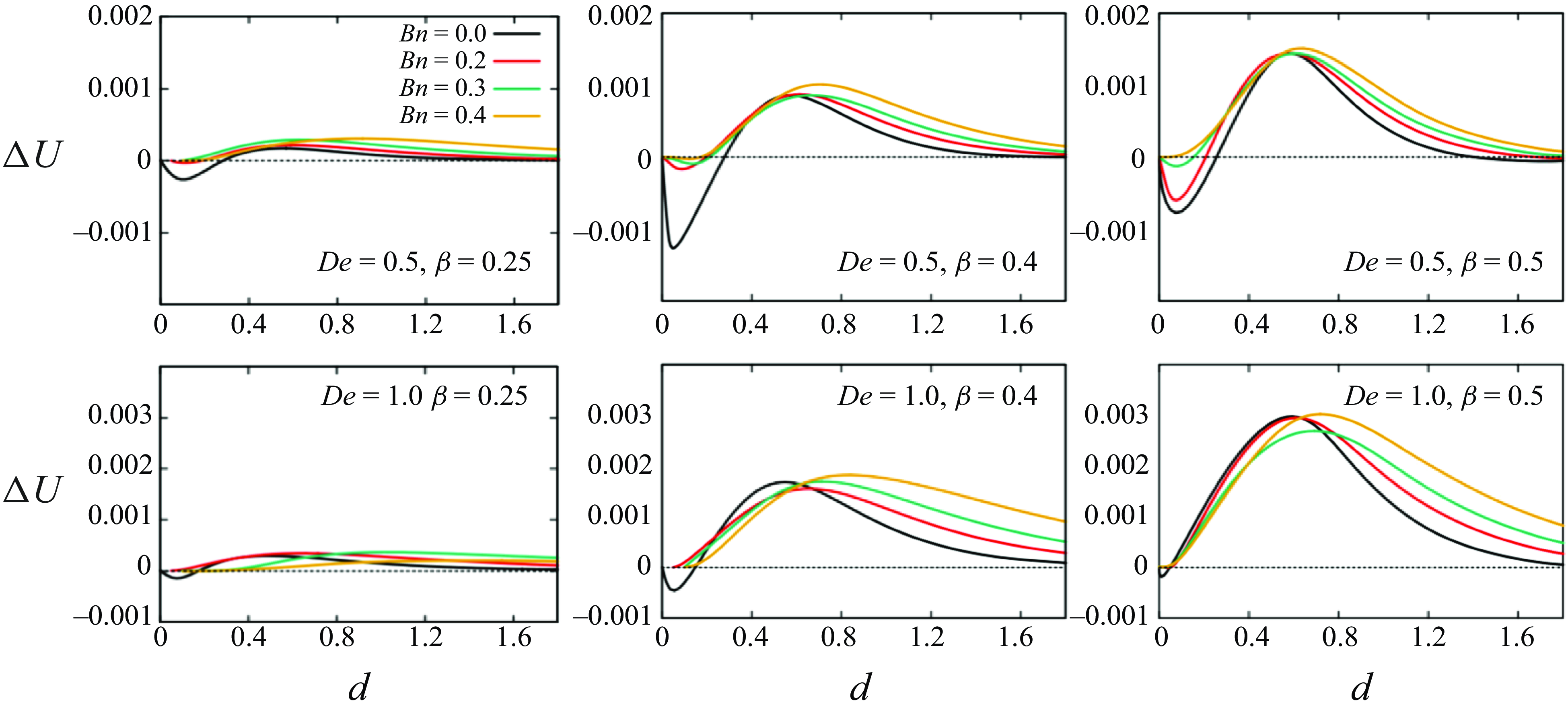
Figure 13. Master curves of the particle relative velocity $\Delta U$
as a function of the inter-particle distance
$\Delta U$
as a function of the inter-particle distance $d$
at De = 0.5 (top row) and 1.0 (bottom row),
$d$
at De = 0.5 (top row) and 1.0 (bottom row), $\beta$
= 0.25 (left column), 0.4 (central column) and 0.5 (right column) and four different Bn values (see legend).
$\beta$
= 0.25 (left column), 0.4 (central column) and 0.5 (right column) and four different Bn values (see legend).
In figure 13, six sets of master curves of the particle relative velocity as a function of the inter-particle distance are shown at De = 0.5 (top row) and 1.0 (bottom row), $\beta$
= 0.25 (left column), 0.4 (central column) and 0.5 (right column), and four different Bn values, as reported in the legends. All the panels on each row (i.e. at given De) have the same scale to emphasise the quantitative differences due to the variation of the confinement ratio: indeed, a higher confinement accelerates the repulsive dynamics between the particles, with the maximum positive relative velocity at
$\beta$
= 0.25 (left column), 0.4 (central column) and 0.5 (right column), and four different Bn values, as reported in the legends. All the panels on each row (i.e. at given De) have the same scale to emphasise the quantitative differences due to the variation of the confinement ratio: indeed, a higher confinement accelerates the repulsive dynamics between the particles, with the maximum positive relative velocity at $\beta =0.5$
being nearly an order of magnitude greater than at
$\beta =0.5$
being nearly an order of magnitude greater than at $\beta =0.25$
. Additionally, the repulsive velocity shows a clear increase with De, as it emerges from the comparison between the panels on each column. Analogous effects are obtained by increasing Bn, indicating that fluid plasticity and elasticity act synergistically to amplify particle repulsion, so facilitating the ordering process in multi-particle systems. This observation is in agreement with previous studies where the yield strain parameter
$\beta =0.25$
. Additionally, the repulsive velocity shows a clear increase with De, as it emerges from the comparison between the panels on each column. Analogous effects are obtained by increasing Bn, indicating that fluid plasticity and elasticity act synergistically to amplify particle repulsion, so facilitating the ordering process in multi-particle systems. This observation is in agreement with previous studies where the yield strain parameter $\varepsilon _{\textit{y}} = \tau _{\textit{y}} \lambda /\eta _{\textit{p}}$
is identified as a measure of the synergy between elastic and plastic effects (Varchanis et al. Reference Varchanis, Haward, Hopkins, Syrakos, Shen, Dimakopoulos and Tsamopoulos2020; Kordalis et al. Reference Kordalis, Varchanis, Ioannou, Dimakopoulos and Tsamopoulos2021; Mousavi et al. Reference Mousavi, Dimakopoulos and Tsamopoulos2024).
$\varepsilon _{\textit{y}} = \tau _{\textit{y}} \lambda /\eta _{\textit{p}}$
is identified as a measure of the synergy between elastic and plastic effects (Varchanis et al. Reference Varchanis, Haward, Hopkins, Syrakos, Shen, Dimakopoulos and Tsamopoulos2020; Kordalis et al. Reference Kordalis, Varchanis, Ioannou, Dimakopoulos and Tsamopoulos2021; Mousavi et al. Reference Mousavi, Dimakopoulos and Tsamopoulos2024).
The influence of yield stress on enhancing elastic effects of complex fluids has been already discussed for single-phase systems (Abdelgawad et al. Reference Abdelgawad, Haward, Shen and Rosti2024), and we posit that a similar rationale applies to our findings. In the yielded regions, where the ‘max’ term multiplying the extra stress tensor in the Saramito–Giesekus constitutive model is non-zero, a division of both sides of the constitutive equation by such term yields a Giesekus model with a locally increased Deborah number compared with the purely viscoelastic case. In the context of single-particle migration, Chaparian et al. (Reference Chaparian, Ardekani, Brandt and Tammisola2020) similarly claimed that EVP materials exhibit more pronounced elastic effects than their viscoelastic counterparts at the same Deborah number. This observation aligns with the argument proposed by Cheddadi et al. (Reference Cheddadi, Saramito, Dollet, Raufaste and Graner2011), who suggested that the plastic nature of the material constrains the extensional deformation behind a moving object, inducing an asymmetry typically observed in viscoelastic fluids when the deformation rate exceeds a critical threshold, which, in turn, is correlated with the yield strain $\varepsilon _{\textit{y}}$
.
$\varepsilon _{\textit{y}}$
.
Notably, when De = 1 (and $\textit{Bn} \gt 0$
), the relative velocity is significantly different from zero even at large inter-particle distances, leading to an increased spacing between particles and enhancing the overall efficiency of the ordering process.
$\textit{Bn} \gt 0$
), the relative velocity is significantly different from zero even at large inter-particle distances, leading to an increased spacing between particles and enhancing the overall efficiency of the ordering process.
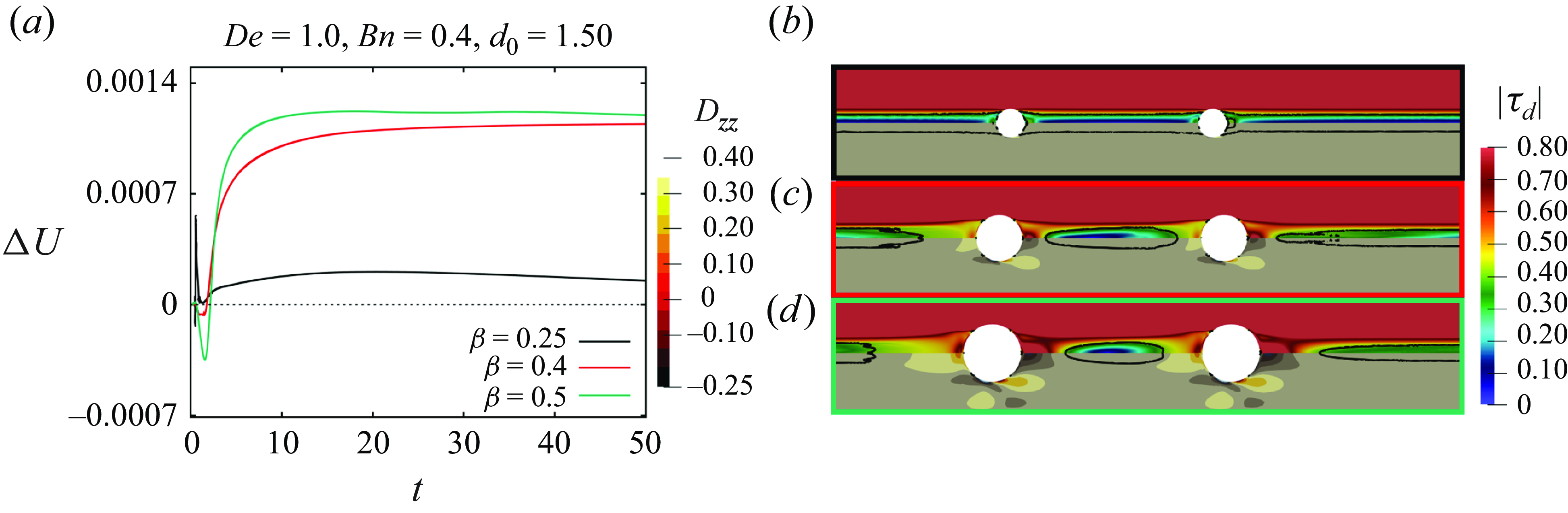
Figure 14. (a) Time evolution of the particle relative velocity $\Delta U$
at De = 1.0, Bn = 0.4,
$\Delta U$
at De = 1.0, Bn = 0.4, $d_{0} = 1.5$
and
$d_{0} = 1.5$
and $\beta$
= 0.25, 0.4, 0.5 (see legend). (b–d) Maps of the second invariant of the deviatoric part of the extra stress tensor
$\beta$
= 0.25, 0.4, 0.5 (see legend). (b–d) Maps of the second invariant of the deviatoric part of the extra stress tensor $|\boldsymbol{\tau }_{\textit{d}}|$
(upper halves) and
$|\boldsymbol{\tau }_{\textit{d}}|$
(upper halves) and $zz$
-component of the rate-of-deformation tensor
$zz$
-component of the rate-of-deformation tensor $D_{\textit{zz}}$
(lower halves) in the fluid around the particles at De = 1.0, Bn = 0.4,
$D_{\textit{zz}}$
(lower halves) in the fluid around the particles at De = 1.0, Bn = 0.4, $d_{0} = 1.5$
,
$d_{0} = 1.5$
, $\beta$
= 0.25, 0.4, 0.5 (from top to bottom) and
$\beta$
= 0.25, 0.4, 0.5 (from top to bottom) and $t = 50$
. The yield surface is indicated with a continuous black line.
$t = 50$
. The yield surface is indicated with a continuous black line.
Figure 14(a) presents the time evolution of the particle relative velocity at $\textit{De} = 1.0$
,
$\textit{De} = 1.0$
, $\textit{Bn} = 0.4$
,
$\textit{Bn} = 0.4$
, $d_{0} = 1.5$
and confinement ratios
$d_{0} = 1.5$
and confinement ratios $\beta$
= 0.25, 0.4 and 0.5. As previously noted, an increase in
$\beta$
= 0.25, 0.4 and 0.5. As previously noted, an increase in $\beta$
corresponds to a higher repulsive velocity. The upper halves of figure 14(b–d) depict the spatial distribution of the second invariant of the deviatoric component of the extra stress tensor in the fluid surrounding the particles at
$\beta$
corresponds to a higher repulsive velocity. The upper halves of figure 14(b–d) depict the spatial distribution of the second invariant of the deviatoric component of the extra stress tensor in the fluid surrounding the particles at $t = 50$
(i.e. the final time point considered in panel a) and
$t = 50$
(i.e. the final time point considered in panel a) and $\beta$
= 0.25, 0.4 and 0.5 (from top to bottom). As
$\beta$
= 0.25, 0.4 and 0.5 (from top to bottom). As $\beta$
increases, the reduced gap between the surfaces of the particles and the channel wall enhances the
$\beta$
increases, the reduced gap between the surfaces of the particles and the channel wall enhances the $zz$
-component of the rate-of-deformation tensor, which is illustrated in the lower halves of figure 14(b–d). This, in turn, results in increased viscoelastic stress. The heightened stress levels in the region between the particles lead to a more pronounced variation in
$zz$
-component of the rate-of-deformation tensor, which is illustrated in the lower halves of figure 14(b–d). This, in turn, results in increased viscoelastic stress. The heightened stress levels in the region between the particles lead to a more pronounced variation in $|\boldsymbol{\tau }_{\textit{d}}|$
, particularly between the front of the trailing particle and the rear of the leading one. In figure 14(b–d), the yield surface is indicated by a solid black line, whose axial extent increases as
$|\boldsymbol{\tau }_{\textit{d}}|$
, particularly between the front of the trailing particle and the rear of the leading one. In figure 14(b–d), the yield surface is indicated by a solid black line, whose axial extent increases as $\beta$
decreases. Specifically, at the lowest
$\beta$
decreases. Specifically, at the lowest $\beta$
value, the suspending phase forms a solid-like region connecting the two particles, leading to a significantly slower variation in their relative velocity. Conversely, at higher
$\beta$
value, the suspending phase forms a solid-like region connecting the two particles, leading to a significantly slower variation in their relative velocity. Conversely, at higher $\beta$
values, the elevated stress levels in the inter-particle region facilitate material yielding. Notably, at
$\beta$
values, the elevated stress levels in the inter-particle region facilitate material yielding. Notably, at $\beta = 0.4$
and
$\beta = 0.4$
and $0.5$
, the stress distributions around the particles are nearly identical, leading to very similar long-term values of the particle relative velocity, as shown by the red and green lines in figure 14(a). Our analysis is restricted to medium confinement ratio (
$0.5$
, the stress distributions around the particles are nearly identical, leading to very similar long-term values of the particle relative velocity, as shown by the red and green lines in figure 14(a). Our analysis is restricted to medium confinement ratio ( $\beta \leqslant 0.5$
) for two primary reasons: first, higher confinement increases the likelihood of clogging, which can disrupt particle ordering, as reported in previous studies (Jeyasountharan et al. Reference Jeyasountharan, D’Avino and Del Giudice2022); second, previous works on particles suspended in viscoelastic materials demonstrated that higher confinement facilitates the lateral migration of particles toward the channel walls (D’Avino et al. Reference D’Avino, Greco and Maffettone2017).
$\beta \leqslant 0.5$
) for two primary reasons: first, higher confinement increases the likelihood of clogging, which can disrupt particle ordering, as reported in previous studies (Jeyasountharan et al. Reference Jeyasountharan, D’Avino and Del Giudice2022); second, previous works on particles suspended in viscoelastic materials demonstrated that higher confinement facilitates the lateral migration of particles toward the channel walls (D’Avino et al. Reference D’Avino, Greco and Maffettone2017).

Figure 15. Particle relative velocity $\Delta U$
as a function of interparticle distance
$\Delta U$
as a function of interparticle distance $d$
for four combinations of the Deborah number De and Bingham number Bn, with the corresponding values indicated in the panels, and five different values of the mobility parameter
$d$
for four combinations of the Deborah number De and Bingham number Bn, with the corresponding values indicated in the panels, and five different values of the mobility parameter $\alpha$
(see legend).
$\alpha$
(see legend).
Finally, we examine the influence of shear thinning, governed by the mobility parameter $\alpha$
in the Saramito–Giesekus constitutive equation. The physical meaning of this parameter is linked to the degree of anisotropy in the drag exerted on the molecules of the liquid (Giesekus (Reference Giesekus1982)). An increase in
$\alpha$
in the Saramito–Giesekus constitutive equation. The physical meaning of this parameter is linked to the degree of anisotropy in the drag exerted on the molecules of the liquid (Giesekus (Reference Giesekus1982)). An increase in $\alpha$
implies that the shear-thinning behaviour manifests itself at lower shear rate. When
$\alpha$
implies that the shear-thinning behaviour manifests itself at lower shear rate. When $\alpha = 0$
, the Saramito–Giesekus model reduces to the standard Saramito model, wherein the yielded material behaves as an Oldroyd-like viscoelastic fluid. In this limiting case, shear-thinning effects are absent, and the molecules experience isotropic drag. To systematically analyse how shear thinning affects the particle pair dynamics, we consider four representative parameter sets, obtained by combining two De values (0.5 and 1.0) and two Bn values (0.1 and 0.2), while maintaining a fixed confinement ratio of 0.4. For each De–Bn couple, we consider 5
$\alpha = 0$
, the Saramito–Giesekus model reduces to the standard Saramito model, wherein the yielded material behaves as an Oldroyd-like viscoelastic fluid. In this limiting case, shear-thinning effects are absent, and the molecules experience isotropic drag. To systematically analyse how shear thinning affects the particle pair dynamics, we consider four representative parameter sets, obtained by combining two De values (0.5 and 1.0) and two Bn values (0.1 and 0.2), while maintaining a fixed confinement ratio of 0.4. For each De–Bn couple, we consider 5 $\alpha$
values. The results of this investigation are summarised in figure 15. At
$\alpha$
values. The results of this investigation are summarised in figure 15. At $\textit{De} = 0.5$
, the results indicate that a lower degree of shear thinning enhances both the repulsive and attractive dynamics, leading to an increase in the magnitude of the undershoot and overshoot. Additionally, the attractive region expands. Notably, for large initial separations (
$\textit{De} = 0.5$
, the results indicate that a lower degree of shear thinning enhances both the repulsive and attractive dynamics, leading to an increase in the magnitude of the undershoot and overshoot. Additionally, the attractive region expands. Notably, for large initial separations ( $d_{0} \gt 1.3$
), the case corresponding to
$d_{0} \gt 1.3$
), the case corresponding to $\alpha = 0$
exhibits a secondary attractive region with a stable equilibrium point. These observations are consistent with previous studies on viscoelastic fluids (D’Avino & Maffettone Reference D’Avino and Maffettone2019). The influence of the Bingham number is primarily quantitative, slightly affecting the magnitude of the undershoot. Specifically, at
$\alpha = 0$
exhibits a secondary attractive region with a stable equilibrium point. These observations are consistent with previous studies on viscoelastic fluids (D’Avino & Maffettone Reference D’Avino and Maffettone2019). The influence of the Bingham number is primarily quantitative, slightly affecting the magnitude of the undershoot. Specifically, at $\textit{Bn} = 0.1$
, the undershoot is more pronounced compared with the case at
$\textit{Bn} = 0.1$
, the undershoot is more pronounced compared with the case at $\textit{Bn} = 0.2$
. At
$\textit{Bn} = 0.2$
. At $\alpha \gt 0.1$
, the master curves nearly collapse on each other. This behaviour is expected, as
$\alpha \gt 0.1$
, the master curves nearly collapse on each other. This behaviour is expected, as $\alpha$
predominantly modulates the minimum shear rate above which shear-thinning effects become significant. The observed increase in the peak relative velocity for both repulsive and attractive interactions is attributed to the higher viscoelastic stress levels and steeper stress gradients generated by fluids exhibiting weaker shear-thinning behaviour. Analogously, the extensional viscosity of the suspending fluid, and thus its extension-rate hardening behaviour, is correlated with the mobility parameter,
$\alpha$
predominantly modulates the minimum shear rate above which shear-thinning effects become significant. The observed increase in the peak relative velocity for both repulsive and attractive interactions is attributed to the higher viscoelastic stress levels and steeper stress gradients generated by fluids exhibiting weaker shear-thinning behaviour. Analogously, the extensional viscosity of the suspending fluid, and thus its extension-rate hardening behaviour, is correlated with the mobility parameter, $\alpha$
. Specifically, increasing
$\alpha$
. Specifically, increasing $\alpha$
results in a decrease in extensional viscosity at high extension rates. This interpretation further supports the explanation that viscoelastic stresses govern the relative displacement of the particles. To further investigate this effect, we conduct an additional set of simulations at an increased Deborah number, while restricting the minimum value of
$\alpha$
results in a decrease in extensional viscosity at high extension rates. This interpretation further supports the explanation that viscoelastic stresses govern the relative displacement of the particles. To further investigate this effect, we conduct an additional set of simulations at an increased Deborah number, while restricting the minimum value of $\alpha$
to 0.005. This constraint arises from the nature of the constitutive model itself: at
$\alpha$
to 0.005. This constraint arises from the nature of the constitutive model itself: at $\alpha = 0$
, the standard Saramito model predicts diverging polymeric stresses beyond a critical threshold of
$\alpha = 0$
, the standard Saramito model predicts diverging polymeric stresses beyond a critical threshold of $\textit{De}$
when the material is subjected to extensional flows, due to the fact that the extensional viscosity grows unbounded.
$\textit{De}$
when the material is subjected to extensional flows, due to the fact that the extensional viscosity grows unbounded.
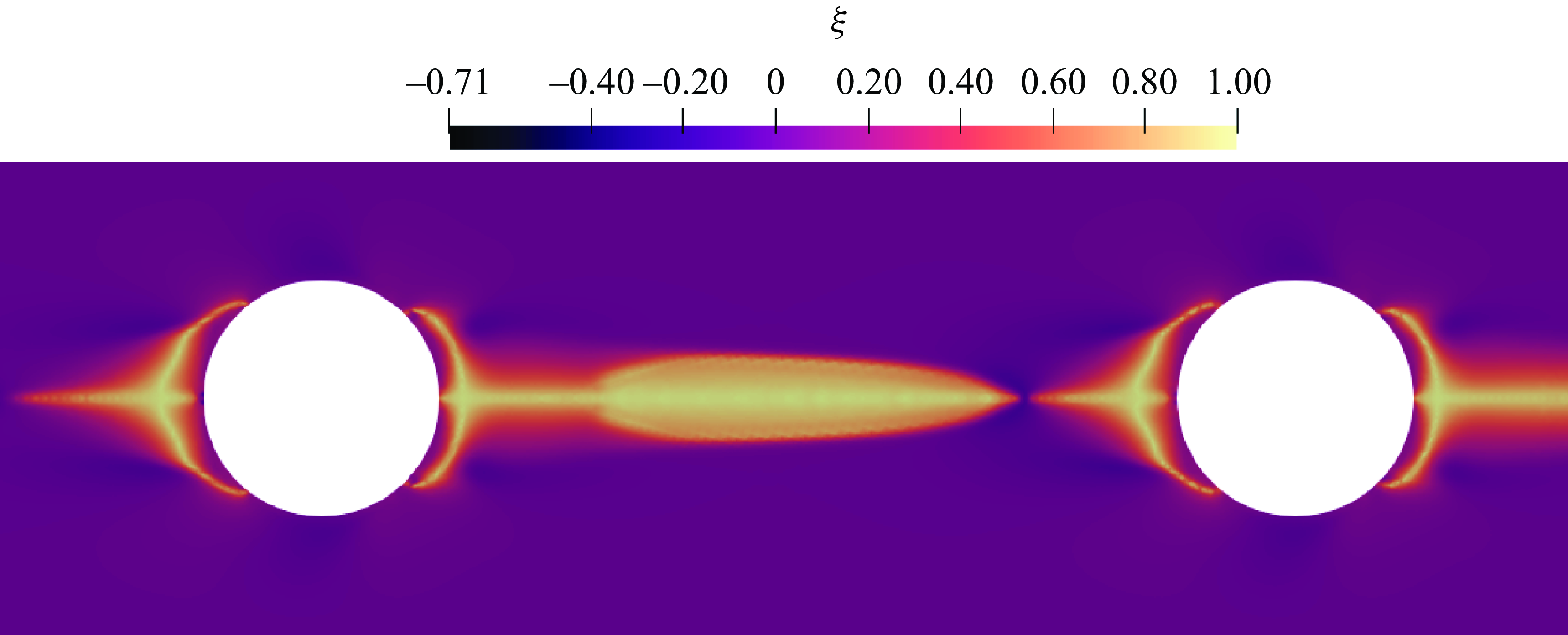
Figure 16. Flow type parameter for a representative case having $\textit{De} = 1$
,
$\textit{De} = 1$
, $\textit{Bn} = 0.4$
,
$\textit{Bn} = 0.4$
, $\beta = 0.5$
and
$\beta = 0.5$
and $d_{0} = 1.50$
.
$d_{0} = 1.50$
.
Indeed, the kinematics of the flow in the interstitial region between particle surfaces is predominantly extensional, as can be characterised using the flow-type parameter $\xi$
(Astarita Reference Astarita1979) defined as
$\xi$
(Astarita Reference Astarita1979) defined as
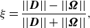 \begin{equation} \xi = \frac {||\boldsymbol{D}|| - ||\boldsymbol{\Omega }||}{||\boldsymbol{D}|| + ||\boldsymbol{\Omega }||}, \end{equation}
where $||\boldsymbol{D}||$
and
$||\boldsymbol{D}||$
and $||\boldsymbol{\Omega }||$
denote the magnitude of the rate-of-deformation tensor and the vorticity tensor, respectively. The local value of this parameter varies between
$||\boldsymbol{\Omega }||$
denote the magnitude of the rate-of-deformation tensor and the vorticity tensor, respectively. The local value of this parameter varies between $-1$
and
$-1$
and $1$
, depending on the dominant flow type. Specifically,
$1$
, depending on the dominant flow type. Specifically, $\xi = 1$
corresponds to purely extensional flow, as
$\xi = 1$
corresponds to purely extensional flow, as $||\boldsymbol{\Omega }||$
is zero,
$||\boldsymbol{\Omega }||$
is zero, $\xi = 0$
indicates shear-dominated flow and
$\xi = 0$
indicates shear-dominated flow and $\xi = -1$
represents purely rotational flow. The map of
$\xi = -1$
represents purely rotational flow. The map of $\xi$
for a representative case (
$\xi$
for a representative case ( $\textit{De} = 1.0$
,
$\textit{De} = 1.0$
, $\textit{Bn} = 0.4$
,
$\textit{Bn} = 0.4$
, $\beta = 0.5$
and
$\beta = 0.5$
and $d_{0} = 1.5$
) is presented in figure 16, indicating that the flow is predominantly extensional along the axis connecting the particles, whereas shear-dominated regions are observed in the gaps between each particle and the lateral wall of the channel. At
$d_{0} = 1.5$
) is presented in figure 16, indicating that the flow is predominantly extensional along the axis connecting the particles, whereas shear-dominated regions are observed in the gaps between each particle and the lateral wall of the channel. At $\textit{De} = 1.0$
, we observe an increase in both repulsive and attractive relative velocities, along with an expansion of the attractive region. However, the stable equilibrium point at larger separation distance,
$\textit{De} = 1.0$
, we observe an increase in both repulsive and attractive relative velocities, along with an expansion of the attractive region. However, the stable equilibrium point at larger separation distance, $d_{\textit{eq}}$
, appears beyond the distance range analysed in this study. While the existence of this equilibrium point is an intriguing finding, its practical relevance remains limited, since, at
$d_{\textit{eq}}$
, appears beyond the distance range analysed in this study. While the existence of this equilibrium point is an intriguing finding, its practical relevance remains limited, since, at $d \gt d_{\textit{eq}}$
, the relative velocity is very small, implying that an extremely long time would be required for the particles to appreciably migrate toward this equilibrium position.
$d \gt d_{\textit{eq}}$
, the relative velocity is very small, implying that an extremely long time would be required for the particles to appreciably migrate toward this equilibrium position.
4. Summary and conclusions
In this work, we perform arbitrary Lagrangian–Eulerian finite-element simulations to investigate the hydrodynamic interactions between two equal non-Brownian rigid spherical particles suspended on the symmetry axis of a cylindrical tube filled with an EVP fluid subjected to pressure-driven flow with a prescribed flow rate.
By examining the dynamics of particle pairs at different values of the operating, constitutive and geometrical parameters that describe the system, we identify master curves of the particle relative velocity as a function of the inter-particle distance. From those, three regimes can be identified, governed by the fluid yield stress and the separation between the particles. At low Bingham number (low yield-stress materials), the particles exhibit attractive interactions at small separation distance, ultimately merging, whereas, at larger separation distance, repulsive interactions are observed, which would promote particle ordering in a multi-particle system. As the Bingham number increases, i.e. the yield stress of the fluid becomes significant, the behaviour at short separation distance is modified, the attractive dynamics being replaced by a stagnation regime, where the particles remain at almost constant distance. In this case, the surfaces of the particles are connected by an unyielded region in which the fluid behaves as a viscoelastic solid, experiencing only minimal deformations. This phenomenon is here reported for the first time and represents a significant deviation from previous studies on polymeric (viscoelastic) suspending fluids (Jeyasountharan et al. Reference Jeyasountharan, D’Avino and Del Giudice2022).
As the Bingham (plasticity) or Deborah (elasticity) number increases, i.e. the yield strain (given by the product of Bingham and Deborah numbers) increases, the repulsive dynamics dominates even at short inter-particle distance, promoting more efficient particle ordering. When the particle confinement ( $\beta$
) is increased, the enhanced deformation rate between the surfaces of the particles and the tube walls correspondingly enhances the stress in the fluid, which, in turn, facilitates the yielding of the material in the region between the particles. This leads to higher relative velocity and the possible formation of ordered structures over shorter channel lengths.
$\beta$
) is increased, the enhanced deformation rate between the surfaces of the particles and the tube walls correspondingly enhances the stress in the fluid, which, in turn, facilitates the yielding of the material in the region between the particles. This leads to higher relative velocity and the possible formation of ordered structures over shorter channel lengths.
Finally, our analysis shows that decreasing the shear-thinning extent amplifies both repulsive and attractive forces, resulting in larger peak relative velocities and an expansion of the attractive region. This effect is attributed to the higher viscoelastic stresses and stress gradients present in less shear-thinning fluids. While a stable equilibrium point at larger interparticle distances is observed in some cases, its practical significance is limited by the extremely low relative particle velocities at such separations.
These findings offer valuable insights for the design of microfluidic devices aimed at non-intrusive particle ordering and controlled structure formation. Future work will extend the analysis to explore interactions involving particle triplets and trains of particles. Additionally, we plan to investigate the hydrodynamic interactions among deformable particles, addressing applications such as the flow cytometry of soft cells.
Acknowledgements
This work is carried out in the context of the project YIELDGAP (https://yieldgap-itn.eu) that has received funding from the European Union’s Horizon 2020 research and innovation programme under the Marie Skłodowska-Curie grant agreement No 955605.
Declaration of interests
The authors report no conflict of interest.


 Open access