


1. Introduction
Many geophysical and environmental flows involve particle-laden plumes, driven by buoyancy, in cross-flows, with important examples including volcanic ash plumes (Sparks et al. Reference Sparks, Bursik, Carey, Gilbert, Glaze, Sigurdsson and Woods1997; Woodhouse et al. Reference Woodhouse, Hogg, Phillips and Sparks2013) and particle plumes produced during deep-sea mining if particle suspensions are discharged from the mining vessel (see figure 1a, cf. Rzeznik, Flierl & Peacock Reference Rzeznik, Flierl and Peacock2019; Drazen et al. Reference Drazen2020). The dynamics of volcanic plumes has been modelled by reference to single-phase buoyant plumes in a cross-flow (e.g. Woodhouse et al. Reference Woodhouse, Hogg, Phillips and Sparks2013, others), following the classical work of Hewett, Fay & Hoult (Reference Hewett, Fay and Hoult1971), Hoult, Fay & Forney (Reference Hoult, Fay and Forney1969) and Slawson & Csanady (Reference Slawson and Csanady1967). These models follow the motion of the centreline of the plume, using equations for the motion parallel and perpendicular to the centreline. A key aspect of such models is the empirical entrainment coefficient associated with the motion along and normal to the centreline of the plume (Hewett et al. Reference Hewett, Fay and Hoult1971; Woodhouse et al. Reference Woodhouse, Hogg, Phillips and Sparks2013; Aubry, Carazzo & Jellinek Reference Aubry, Carazzo and Jellinek2017a; Aubry et al. Reference Aubry, Jellinek, Carazzo, Gallo, Hatcher and Dunning2017b). The entrainment coefficients in the models have been tested with laboratory experiments by comparing the plume trajectory with the model predictions (Carazzo et al. Reference Carazzo, Girault, Aubry, Bouquerel and Kaminski2014; Aubry et al. Reference Aubry, Carazzo and Jellinek2017a,Reference Aubry, Jellinek, Carazzo, Gallo, Hatcher and Dunningb).

Figure 1. (a) Schematic of a deep-sea mining situation, with a particle-laden discharge plume; (b) experimental analogue system.
There have been some experiments modelling the dynamics of particle-laden plumes in a still ambient. These experiments have shown that, provided the fall speed of the particles is smaller than the convective speed of the plume, based on the buoyancy associated with the particle load, then the flow develops as a convective plume, entraining and mixing ambient fluid (cf. Mingotti & Woods Reference Mingotti and Woods2019). Less is known about the transport and sedimentation of particles from plumes in a cross-flow, and we are not aware of any detailed experiments modelling the dynamics of such plumes. There have, however, been a number of experimental studies of bubble plumes in a cross-flow (e.g. Socolofsky & Adams Reference Socolofsky and Adams2002; Murphy et al. Reference Murphy, Xue, Sampath and Katz2016), which have identified that, as the flow moves downstream, there is separation of the bubbles and fluid, and this has some analogy with the separation of particles and fluid discussed in the present paper. These works focussed on describing and quantifying the distribution of the bubbles/droplets in the plume, but did not develop a criterion to determine the depth of separation of the fluid and bubbles in the plume. Furthermore, the dynamics of bubble plumes can be more complex owing to bubble merger and break up, and also the possible range of bubble sizes.
In order to explore the dynamics of particle-driven plumes, we have therefore carried out a series of simplified laboratory experiments of dense particle-driven plumes, and this forms the main topic of this paper. However, before launching into these new experiments, we first carry out a series of reference experiments of a dense single-phase plume driven by an aqueous saline solution supplied to a reservoir of fresh water. These experiments provide new insight into the dynamics of a turbulent plume in a cross-flow, in particular demonstrating that, after a transition region just beyond the source, the horizontal speed of the plume fluid matches that of the ambient current. Subsequently, the dynamics and entrainment into the plume can be described in terms of the vertical motion of the plume. We establish that this vertical motion is directly analogous to the dynamics of a line thermal produced by the release of a finite volume of dense fluid in a stationary ambient. We illustrate that the motion can be described using a simple model for the trajectory of the centreline of the plume, coupled with an entrainment coefficient associated with the vertical motion of the flow (cf. Hewett et al. Reference Hewett, Fay and Hoult1971; Chu Reference Chu1975; Woitischek et al. Reference Woitischek, Mingotti, Edmonds and Woods2021).
We then present a series of new experiments to explore the dynamics of dense particle-driven plumes in a cross-flow. In particular, we compare the trajectory of the particle-driven plume composed of fresh water and particles migrating through a tank filled with fresh water with our simplified model for a single-phase plume of the same source buoyancy flux, but composed of an aqueous saline solution moving through a tank filled with fresh water. Based on this comparison we establish a quantitative model for the control on the separation of the particles from the plume fluid. For simplicity, we assume the density of the fluid in the particle plumes equals that of the surrounding ambient fluid, so that the buoyancy in the plume is purely associated with the presence of the relatively dense particles. Also, in each of the present experiments, we use particles of a given size and hence well-characterised fall speed. By using the simplified model of the plume, together with some experiments in which we have dyed the source fluid in the plume, we present a new quantitative criterion for the depth at which particle–fluid separation occurs, and we illustrate the trajectory of the particles and also the plume fluid pre- and post-separation. We also demonstrate that, with the particle plumes, even though the particles appear to form localised clusters as they settle through the ambient fluid after separating from the plume, the fall speed of the particles closely approximates the sedimentation speed of individual particles, rather than some larger convective fall speed.
In § 7, we consider the implications of our results for the dispersal of particles in plumes produced during deep-sea mining.
2. Laboratory experiments
To model plumes in a cross-flow, we follow an experimental approach used in earlier studies (e.g. Hewett et al. Reference Hewett, Fay and Hoult1971; Chu Reference Chu1975) and use a moving source of dense fluid in a static tank of ambient fluid; by Lagrangian transformation, we expect the moving dense plume which forms to be equivalent to the plume which develops when there is a stationary source of dense fluid in a uniformly translating body of fluid. The experimental system consisted of a tank of length 245 cm, width 60 cm and depth 35 cm, in which there is a moving source which runs along a bespoke track at the top of the tank with a constant, but controllable speed. The source was connected to a stirred reservoir containing the source fluid, which was supplied to the tank using a peristaltic pump (Watson Marlow). The tank was filled with fresh water, and an electroluminescent light sheet (LightTape by Electro-LuminiX Lighting Corp.) was placed behind the tank. A Nikon D5300 camera was used to record the experiments, with a frame rate of 50 f.p.s. (figure 1b).
A series of experiments were carried out with different flow rates and traverse speeds. Initially, we carried out a series of experiments using a dyed aqueous saline solution for the source fluid, and we analysed the ensuing dense plumes in order to quantify the trajectory of the centreline and the entrainment coefficient of the flow, for comparison with the simplified single-phase model of a buoyant plume in a cross-flow. We also carried out a series of experiments in which we released a finite volume of dense fluid from a line source, 1.6 m long, located just below the surface of the tank, in order to compare the motion of and entrainment into the plume with that of the line thermal produced by a line source of dense fluid. We then carried out a systematic series of experiments using mixtures of fresh water and silicon carbide particles (Carborex by Washington Mills) as the source fluid. In order to ensure a uniform suspension of particles in the source fluid, we used a stirrer in the source tank, which produced a uniform suspension of particles in the source fluid. Table 1 summarises the conditions of the experiments.
Table 1. Conditions of the experiments. Here,  $Q$ (m $^3$ s $^{-1}$) is the source volume flux; $g'$ (m s $^{-2}$) is the reduced gravity of the source fluid; $B$ (m $^4$ s $^{-3}$) is the source buoyancy flux; $u$ (m s $^{-1}$) is the speed of the moving source; $d$ (m) is the mean particle diameter; $v$ (m s $^{-1}$) is the particle settling speed; $\varPhi$ is the particle volume fraction in the suspension. In experiments 28–33, a saline solution was used as the source fluid. The inner radius of the source was fixed across the whole set of experiments, $r_0=3\times 10^{-3}$ m. The density of the silicon carbide particles was also fixed at $\rho _p=3206$ kg m $^{-3}$.

3. Experimental observations: single-phase plumes in a cross-flow and line thermals in a stationary ambient
In figure 2, we present images of a typical saline plume in a cross-flow, both (a) an instantaneous image and (b) the associated time average, averaged over 20 s, plotted in false colour and shown in the frame of the moving source. In this time-averaged image, the vertical distribution of the dye along each vertical line through the plume has been fit with a Gaussian distribution, leading to estimates of the position of the centre and the standard deviation of the plume as a function of distance downstream (see figure 2c). The instantaneous image (figure 2a) illustrates the somewhat irregular shape of the lower descending front, while the upper front of the plume is much smoother (cf. Hewett et al. Reference Hewett, Fay and Hoult1971). In a number of experiments, the colour of the dye was changed part way through the experiment. Figure 2(d) shows five images captured at regular time intervals during one of these experiments in the frame of the laboratory. For each frame captured during this experiment, we calculated the vertical average of the dye colour in the plume, as a function of time. A time series of this vertical average, in the frame of the laboratory, is shown in figure 2(e). Figure 2(d,e) illustrates that the location of the change of colour of the dye remains approximately fixed in the laboratory frame, suggesting that, soon after issuing from the nozzle, the lateral motion of the plume relative to the ambient fluid decreases to zero and, to leading order, the plume may be regarded as descending vertically through the ambient fluid, as it moves downstream with the ambient fluid. This observation suggests that the entrainment of ambient fluid arises owing to the vertical motion of the plume, and hence may be parameterised by a single entrainment coefficient, as assumed by Chu (Reference Chu1975).

Figure 2. (a) Instantaneous image captured during a saline experiment. (b) Time average of all the images captured during the experiment in the source frame, plotted in false colour. (c) Solid lines are used to plot three vertical dye concentration profiles as a function of height in the tank. Dotted lines illustrate the best-fit Gaussian for each of these profiles. (d) Five images recorded at regular time intervals  $\Delta t=1.30$ s during an experiment in which the colour of the dye was changed part way through the experiment. (e) Time series of the vertically averaged dye concentration profiles recorded during the same experiment.
In order to test this observation in more detail, we have run a series of experiments in which a finite volume (200 ml) of dense saline solution, with buoyancy  $g'$ ranging between 0.15 and 1.09 m s $^{-2}$, was released from a horizontal line source, 1.6 m long, located 2 cm below the surface of the tank. After release, the fluid produced a line thermal which gradually descended to the base of the tank while entraining ambient fluid. In figure 3(a), we illustrate a series of images of a representative line thermal as a function of time and in panel (b), we present a time series of the horizontally averaged light intensity of this thermal, as a function of depth and time, illustrating how the thermal descends through the tank. This image is remarkably similar in form to figure 2(b), although representing a different flow, and in § 4, we compare the depth–time trajectories and the rate of entrainment of these different flows in detail.

Figure 3. Results of a single-phase line thermal experiment, in which 200 ml of fluid with buoyancy  $g'=0.15$ m s $^{-2}$ was released from a source 1.6 m long. (a) Series of 4 images captured at times 2 s, 7 s, 17 s and 27 s after the beginning of the experiment and plotted in false colour to illustrate the concentration of dye in the line thermal fluid. (b) Time series of the horizontally averaged dye concentration profiles, showing the trajectory of the thermal fluid as it sinks to the bottom of the tank.
4. Modelling the time-averaged flow: single-phase plumes and line thermals
Numerous models have been proposed to capture the dynamics of turbulent single-phase plumes in a cross-flow, following the pioneering work of Hewett et al. (Reference Hewett, Fay and Hoult1971). We now compare the results of the experiments discussed in § 3 with the simplified picture in which we assume that following an initial adjustment, the plume fluid moves downstream with the ambient fluid, as suggested by the experiments shown in figure 2(d,e). We compare the model with the trajectory and entrainment into a line thermal produced by the release of a finite volume of dense fluid from a line source. We adopt this model helping to interpret the particle plume experiments later in the paper. If the horizontal speed of the plume fluid matches that of the ambient fluid,  $u$, (figure 2d,e) then the horizontal position of the plume centreline, $x$, increases as
 \begin{equation} \frac{\textrm {d}\kern0.7pt x}{\textrm{d}t}=u. \end{equation}
The downward motion can be described in terms of a speed  $w=\textrm {d}z/\textrm {d}t$ and the effective radius $r$ of the vertical cross-section of the plume of area $A={\rm \pi} r^2$. This increases through mixing with ambient fluid as it descends through the ambient fluid according to the relation (cf. Turner Reference Turner1969; Hewett et al. Reference Hewett, Fay and Hoult1971)
 \begin{equation} w\frac{\textrm{d}r}{\textrm{d}z}=\beta w, \end{equation}
where  $\beta$ is an entrainment coefficient. The vertical momentum of the thermal evolves as
 \begin{equation} \frac{\textrm{d}\left(r^2 w\right)}{\textrm{d}t}=\gamma g' r^2. \end{equation}
Here,  $g'$ is the buoyancy and $\gamma <1$ is a factor which accounts for the momentum associated with the added mass of the ambient fluid which is displaced as the plume fluid sinks, combined with any circulation directed along the axis of the plume, whose angular velocity is expected to be proportional to $w/r$. This has some analogy to the circulation which develops in an axisymmetric buoyant thermal (cf. Turner Reference Turner1969; Mott & Woods Reference Mott and Woods2009). If the source has buoyancy flux $B$, then the buoyancy flux per unit length is $g'r^2 = B/u$, and (4.3) can be re-expressed in the form
 \begin{equation} \frac{\textrm{d}\left(r^2 w\right)}{\textrm{d}t}=\frac{\gamma B}{u}, \end{equation}
and so
 \begin{equation} r^2 w = \frac{\gamma B}{u}t+r^2_0w_0. \end{equation}
Equation (4.2) leads to the result
 \begin{equation} r=r_0+\beta \left(z-z_0\right), \end{equation}
where  $z_0$ is a virtual origin which we set to have value $z_0=r_0/\beta$. Combining (4.5) and (4.6) and integrating in time, we then obtain
 \begin{equation} z^3=\frac{3\gamma B}{2\beta^2u^3}x^2+\frac{3r^2_0w_0}{\beta^2 u} x+z^3_0, \end{equation}
for the depth of the centreline of the plume as a function of distance downstream, where we have used the substitution  $x=ut$. From (4.7), we see that the buoyancy transition length $L$, which corresponds to the distance downstream beyond which the buoyancy controls the flow, is given by
 \begin{equation} L=\frac{2 u^2 r_0^2 w_0}{\gamma B}, \end{equation}
which in the present experiments has value of order 0.1 m. Since the majority of the plumes we have studied extend for lengths of 1 m or more and  $z_0\sim 0.01$ m, we expect that to leading order the trajectory is given by (cf. (4.7))
 \begin{align} z^3&\approx\dfrac{3\gamma B}{2\beta^2u^3}x^2, \end{align}
 \begin{align} \text{or alternatively} \quad z^3&\approx \dfrac{3\gamma}{2\beta^2}\left(\dfrac{B}{u}\right)t^2. \end{align}
Matching this relation with our experimental data, we find the best fit agreement when
 \begin{equation} \frac{\gamma}{\beta^2}=0.87\pm 0.05, \end{equation}
as shown in figure 4(a), in which we compare the experimental data for  $z$ (vertical axis) as a function of $(B/u^3)^{1/3} x^{2/3}$ (cf. (4.9a); horizontal axis) for experiments 28–33 in table 1. This value is consistent with the values presented by Hewett et al. (Reference Hewett, Fay and Hoult1971) and Chu (Reference Chu1975). Combining (4.9) and (4.10), it may be shown that the vertical speed in the plume follows the relation
 \begin{equation} \frac{\textrm{d}z}{\textrm{d}t}=w=0.76 \left( \frac{B}{uz}\right)^{1/2}. \end{equation}
The pink dashed line in figure 4(a) shows the measured depth  $z$ of the centreline of the horizontal average of the line thermal illustrated in figure 3(b) (vertical axis) as a function of the model prediction given by (4.9b), $(B/u)^{1/3} t^{2/3}$ (horizontal axis). It is seen that the experimental data for the line thermal also lie close to the straight dashed line predicted by (4.9b).

We have measured the light intensity along each vertical line through the time-averaged plume, in the frame of the source; to good approximation this follows a Gaussian distribution, and the increase of the standard deviation along each vertical line in the plume as a function of the depth of the centre of the plume is shown in figure 4(b). This suggests that the standard deviation is proportional to the depth of the centreline according to the relation
 \begin{equation} \sigma=\left(0.40 \pm 0.05\right) z. \end{equation}
If we define the plume radius as equal to the standard deviation, this implies
 \begin{equation} \beta=0.40\pm0.05 \ \text{and so} \ \gamma = 0.15 \pm 0.03. \end{equation}
This value of  $\beta$ is consistent with the results of earlier experiments (e.g. Chu Reference Chu1975). The entrainment process is dominated by the double vortex structure of the descending line thermal, as the ambient fluid is swept around the descending cloud. Analysis of the time series image of the horizontal average of the line thermal shown in figure 3(b) also indicates that $\beta = 0.4 \pm 0.04$ for the case of the line thermal. This establishes the analogy between the dynamics of a line thermal in stationary fluid and that of a steady plume in a cross-flow, where the plume fluid moves laterally with the ambient current as it falls vertically through the ambient fluid (4.8).
5. Experimental observations: particle-driven plumes in a cross-flow
We now present the results of a series of particle-driven plume experiments, which were carried out using the same experimental setup described in § 2, using a suspension of silicon carbide particles in fresh water as the source fluid.
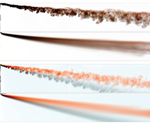
In figure 5, we present images from two different particle plume experiments, in which a suspension of black particles and red-dyed fluid issues from the source. The experiments show the case of (a,b) small particles (experiment 17 in table 1) and (c,d) larger particles (experiment 1), with panels (a,c) illustrating two instantaneous images as captured during each experiment and panels (b,d) illustrating the time averages in the frame of the source. It is seen that with the small particles of a mean diameter 45  $\mathrm {\mu }$m (see table 1), owing to the very small sedimentation speed, the particles and fluid remain coupled in space, and the shape of the plume resembles the shape of the flow seen in figure 2(a); we explore this quantitatively below (§ 6). In contrast, in panels (c,d), with the larger particles of a mean diameter 165 $\mathrm {\mu }$m (see table 1) and a relatively large sedimentation speed compared with the plume speed, there is a clear separation of the fluid and particles as the flow moves downstream relative to the source. Here, we note that, although apparently organised in clusters of high and low particle concentration along the plume, the particles appear to follow a straight line trajectory, as if simply sedimenting through the fluid, rather than following the coherent convective motion suggested in panels (a,b) (see § 6).

Figure 5. (a,c) Instantaneous and (b,d) time-averaged images of two particle plumes. In (a,b) the plume was laden with small particles of a mean diameter 45  $\mathrm {\mu }$m (experiment 17 in table 1) which do not separate from the red-dyed fluid. In (c,d) the plume was laden with larger particles of a mean diameter 165 $\mathrm {\mu }$m (experiment 1) which separate from the dyed plume fluid and fallout. The photographs in panels (a,c) were captured 15.4 s after the beginning of each experiment.
6. Modelling the time-averaged flow: particle-driven plumes
In particle plumes, the reduced gravity of the suspension of particles in a neutrally buoyant fluid can be written
 \begin{equation} g'=\varPhi \frac{\rho_p-\rho_{amb}}{\rho_{amb}}g, \end{equation}
where  $\rho _p$ is the density of the particles, $\rho _{amb}$ is the density of the ambient fluid, $g$ is the acceleration of gravity and $\varPhi$ is the particle volume fraction in the suspension (see table 1), with a buoyancy flux given by $B=g'Q$. The initial stages of motion of the flow are very similar to those of the saline plume. For the smallest particle sizes of mean diameter 17 $\mathrm {\mu }$m (experiments 21–24 in table 1), the motion resembles that of a single-phase plume throughout the tank; the width of the plume increases with depth in a similar way to the saline plume (figure 6a), and the trajectory of the centre of the plume follows the prediction of (4.7), as may be seen in figure 6(b) by comparing the black dashed line (model) and the lines labelled 20 and 24 corresponding to plumes with small particles. However, (4.9b) shows that the vertical speed of the plume gradually decreases with depth and so eventually with larger particles, the plume speed will become comparable to the fall speed of the particles. As this happens, the particles begin to separate from the original plume fluid (see figure 5c,d). The subsequent motion of the particles suggests that the descent speed of the centre of the particle cloud matches the particle Stokes settling speed, $v$, with the time-averaged centre of the particle cloud following a trajectory with gradient
 \begin{equation} \frac{\textrm {d}\kern0.7pt x}{\textrm{d}z}=\frac{u}{v}. \end{equation}
Figure 6. (a) Growth of the radius of the small-particle plume with depth (experiments 21–24 in table 1), which is very similar to the saline plume (see figure 4b). (b) Plot of the measured depth of the centreline of the particle plume with the model prediction for a single-phase plume with the same buoyancy flux (4.7). (c) Comparison of the simple sedimentation trajectory  $z=xv/u$ (6.2) with data from a series of experiments using particles of different sizes (experiments 4, 8, 12, 16, 20 and 24 in table 1).
In order to demonstrate this change in behaviour, in figure 6(b,c) we present the trajectory of the centre of the particle cloud for a series of particle plumes with the same buoyancy but different fall speeds of the particles (experiments 4, 8, 12, 16, 20 and 24 in table 1). In panel (b), we have scaled the trajectory relative to the model (4.7), and in panel (c) we have scaled the trajectory relative to the simple sedimentation law (6.2). It is seen that, in panel (b), the trajectories of the particles follow that of the plume model (4.7) for the small particles of mean diameter  $d<45\,\mathrm {\mu }$m (see table 1). As the particle size increases, corresponding to experiments 16, 12, 8 and 4 in table 1, the trajectories depart from the single-phase plume model at points progressively closer to the source. The data show that the particles subsequently descend through the tank faster than given by the convective flow speed of the equivalent single-phase plume. In panel (c), we see that for the larger particles of mean diameter $d>145\,\mathrm {\mu }$m, the centre of particle cloud follows the ballistic trajectory (6.2). However, for the smaller particles, in the near-source region the particles descend with progressively larger speeds relative to their sedimentation speed, and we infer from panel (b) that these correspond to the convective speed of the plume.
The depth of the transition from plume-driven flow to separated flow,  $z^*$, can be defined as the depth of the centre of the particle cloud at which the upper edge of the particle cloud intersects the lower edge of the original dyed plume fluid (see figure 7a). In practice, we estimate $z^*$ by finding the depth at which the point Ⓐ, a distance equal to one standard deviation of the vertical distribution of particles above the centre of the particle cloud, coincides with the point Ⓑ, a distance equal to one standard deviation of the vertical distribution of dye below the centre of the dye cloud (dotted and dashed white lines in figure 7a, respectively). Physically, we expect that at this depth the vertical plume speed, $w$, equals a constant fraction of the particle fall speed, $v$
$v$
 \begin{equation} v=\lambda w, \end{equation}
so that
 \begin{equation} z^*=\frac{\lambda^2}{v^2} \left(\dfrac{2 \gamma B}{3 \beta^2 u}\right). \end{equation}
In figure 7(b), we show the measured value of  $z^*$ as a function of $B/(v^{2}u)$. The data suggest that
 \begin{equation} \lambda=0.92\pm0.08. \end{equation}
We note that, for consistency of this model, it is required that the adjustment length scale  $L$ given by (4.8) is small compared with the transition distance $x^*=uz^*/v$ so that the separation of the particles and plume fluid only occurs after the buoyancy dominates the motion of the plume. Using the results shown in figure 7(b), we estimate that in our experiments the ratio $L/x^*$ is of order $10^{-1} - 10^{-2}$ in accord with this constraint.

Figure 7. (a) Time-averaged image of a plume containing dyed fluid (red) and large particles (black). The white dotted line denotes the locus of points one standard deviation above the centreline of the particles, while the white dashed line denotes the locus of points one standard deviation below the centreline of the dye. We define the transition point  $(x^*, z^*)$ as the point where these two lines cross. (b) Comparison of the model prediction of the depth of the particle separation (6.4) with the experimental measurement, for experiments 1–16 in table 1.
7. Implications for particle plumes in nature
The above modelling identifies how a particle plume in a cross-flow progressively dilutes with distance from the source, and that this leads to a gradual decrease in the vertical convective speed of the flow until eventually this falls below the particle fall speed. As this happens, particles can sediment from the lower surface of the flow. Subsequently, the particles descend with their individual particle settling speed, advancing ahead of the original plume fluid. This observation is important for assessing the environmental impact of such a particle-laden plume, given that the fate of the original suspension fluid as well as the particles may be of interest.
One fascinating feature of the process is that the particles arrange themselves into a series of discrete particle clouds along the axis of the main plume (e.g. see figure 5c). These local particle clouds appear to develop in the early stages of the flow, while the vertical convective motion dominates the vertical transport of the particles, and analogous features may also be seen in the single-phase plumes (figure 2a). There is a continual coarsening of these structures as the plume descends, as may be seen in figure 8(a). Here, we show a time series of three vertical lines of pixels located at different distances downstream from the source in the frame of the source (figure 8a). It is seen that in each image, there are regions of high and low concentration, consistent with the discrete particle clouds as seen in figure 5(a,c). We note that these discrete particle clouds appear gradually to merge and become of greater size as the plume descends. We characterise the horizontal length scale of the structures,  $\delta$, and the associated frequency $f = u/\delta$, as the plume sinks by analysing the time series images shown in figure 8(a) using the Matlab fast Fourier transform algorithm. Figure 8(b) shows that for eight experiments $\delta$ increases linearly with $z$ for both particle and the equivalent single-phase plumes according to the relation
 \begin{equation} \frac{\delta}{z}=0.84\pm0.10. \end{equation}
It is interesting that these clouds do not seem to influence the descent speed of the particles once they have sedimented from the plume. To good approximation, the descent speed is given by the sedimentation speed of the particles (figure 6c). This contrasts with the convective sedimentation of particles described by Hoyal, Bursik & Atkinson (Reference Hoyal, Bursik and Atkinson1999) from a large areally distributed source of particle-laden fluid, in which the particle clouds descended significantly faster than the particle fall speed.

Figure 8. (a) Time series of three vertical lines of pixels at different distances from the source, illustrating the sedimenting structures in the plume. It is seen that the scale of the structures increases with depth and distance downstream. (b) Measured length scale of the sedimenting structures,  $\delta$, as a function of depth, $z$, for a number of saline and particle experiments (n. 1, 2, 5, 6, 30, 31, 32 and 33 in table 1).
In the context of deep-sea mining, the typical discharge rates from a surface vessel are expected to be in the range  $0.001 - 0.1$ m $^3$ s $^{-1}$, with particle loads of 1 %–10 %. With sediment density in the range $2000 - 3000$ kg m $^{-3}$, we infer buoyancy fluxes may have values $0.01 - 1.0$ m $^4$ s $^{-3}$. With current speeds of order $0.01 - 0.1$ m s $^{-1}$, the buoyancy transition length (4.8) is typically ${<}1 - 10$ m, so the analysis described in this paper applies. The particle separation depth below the source, according to (6.4), would then be in the range of 10–1000 m, for particles with fall speeds of $0.1 - 0.01$ m s $^{-1}$. The fate of the particles subsequently involves direct sedimentation through the water column, and this provides constraints on the settling time of the particles through the water column as well as the depth of any contaminated fluid which is carried downwards by the initial convective plume type motion. As an idealised example, if the particles fall 100 m in the plume and then separate and sediment through the remainder of the water column, the travel time to sink 1000 m would be in the range 3–30 h. With current speeds of $0.01 - 0.1$ m s $^{-1}$, this suggests the particles may be dispersed by the current over lateral scales of 1–10 km from the source.
It is also of interest to observe that the background stratification of the water column imposes a second length scale on the flow, given in terms of the Brunt-Väisälä frequency,  $N$,
$N$,
 \begin{equation} z=\omega \left(\frac{B}{u}\right)^{{1}/{3}} N^{-{2}/{3}}, \end{equation}
where  $\omega$ is an empirical constant which has been estimated to have value of order 2 (Briggs Reference Briggs1975; Devenish et al. Reference Devenish, Rooney, Webster and Thomson2010). In the deep ocean, where $N\approx 10^{-2} - 10^{-3}$ s $^{-1}$, this leads to depths of 10–1000 m. We deduce that particle plumes composed of smaller particles may become arrested by the stratification prior to sedimenting from the flow. This would lead to a particle–fluid intrusion forming within the water column, from which particles then sediment into the deeper waters (cf. Mingotti & Woods Reference Mingotti and Woods2019, Reference Mingotti and Woods2020), although being influenced by the cross-flow. In contrast, for the larger particle plumes, with particle settling speeds of order 0.1 m s $^{-1}$, the particles may sediment from the plume in the first 10–100 m, and will then settle through the water column as illustrated in the experiments of the present paper, with much less influence of the stratification.
Comparing (6.4) and (7.2), we find that the separation will occur prior to the effects of stratification being important if
 \begin{equation} 0.24 \left(\frac{BN}{u}\right)^{{2}/{3}} \frac{1}{v^2} < 1. \end{equation}
The ratio of the separation and intrusion heights as a function of particle settling speed are shown in figure 9 for the cases  $N = 0.01$, 0.001 and 0.0001 s $^{-1}$, in the case $B/u = 1$. In this figure, we see that plumes containing particles with larger fall speeds or in more weakly stratified environments, are likely controlled by the dynamics described in this work, while the effects of stratification become more significant for smaller particles.

Figure 9. Ratio of the separation and intrusion heights in a particle plume as a function of the particle fall speed, for the cases  $N = 0.01$, 0.001 and 0.0001 s $^{-1}$, in the case $B/u = 1$.
In the context of volcanic plumes, the dynamics is more complex owing to the heat transfer between the solid particles and the host fluid in the plume, leading to the buoyancy of the cloud being associated with both the plume fluid and the particles. We are presently exploring this dynamics, building on the present understanding of the controls on particle separation in a plume in cross-flow.
In closing, we note that the present work has focussed on plumes laden with a monodisperse suspension of particles of a single size. In practice, there may be a range of particle sizes in suspension in the plume. The present work suggests that there will be a gradual loss of particles from the plume as the plume descends and slows down, with the largest particles sedimenting first. As particles sediment from the plume, the buoyancy of the residual plume will decrease, further reducing the plume speed. We plan to explore this dynamics in a further contribution.
Funding
This research received no specific grant from any funding agency, commercial or not-for-profit sectors.
Declaration of interests
The authors report no conflict of interest.
Data availability
The data that support the findings of this study are available from the corresponding author on reasonable request.


 Open access