


1. Introduction
There has been considerable interest recently in understanding the hydrodynamic interactions between flapping wings in moderate to high Reynolds number flows, for which inertial effects are relevant. Apart from scientific curiosity, this interest is motivated by numerous biological and engineering applications. Specifically, understanding why fish swim in schools (Pavlov & Kasumyan Reference Pavlov and Kasumyan2000) and birds fly in flocks (Bajec & Heppner Reference Bajec and Heppner2009) has been of long-standing interest to biologists and physicists studying collective behaviour in animal groups. While many studies have investigated how social interactions between fish may mediate schooling behaviour (Tunstrøm et al. Reference Tunstrøm, Katz, Ioannou, Huepe, Lutz, Couzin and Ben-Jacob2013; Swain, Couzin & Leonard Reference Swain, Couzin and Leonard2015; Jolles et al. Reference Jolles, Boogert, Sridhar, Couzin and Manica2017), the so-called Lighthill conjecture posits that orderly formations in schools may arise passively due to hydrodynamic interactions, instead of requiring active control or decision making (Lighthill Reference Lighthill1975). The underlying mechanisms behind flow-induced collective behaviour could have applications to the next generation of biomimetic underwater vehicles, which self-propel using mechanisms inspired by fish locomotion (Triantafyllou, Triantafyllou & Yue Reference Triantafyllou, Triantafyllou and Yue2000; Geder et al. Reference Geder, Ramamurti, Edwards, Young and Pruessner2017).
Field observations of the formations adopted by fish schools are diverse and typically vary between species (Pavlov & Kasumyan Reference Pavlov and Kasumyan2000). For instance, some fish species (e.g. minnow, bream, saithe, herring) tend to adopt lattice-like schooling formations, while others (e.g. cod) adopt more disordered configurations (Pitcher Reference Pitcher1973; Partridge et al. Reference Partridge, Pitcher, Cullen and Wilson1980). Recent laboratory experiments have revealed that red nose tetra fish may adopt different lattice-like formations when they school (Ashraf et al. Reference Ashraf, Godoy-Diana, Halloy, Collignon and Thiria2016, Reference Ashraf, Bradshaw, Ha, Halloy, Godoy-Diana and Thiria2017). Our paper is concerned with the simplest of these formations, the so-called in-line formation, in which the line connecting the fish is in the swimming direction. Indeed, fish have been observed to swim in linear chains (Gudger Reference Gudger1944), and pairs of goldfish have recently been observed to school in an in-line formation in which the follower beats its tail to synchronise with the oncoming vortices shed by the leader (Li et al. Reference Li, Nagy, Graving, Bak-Coleman, Xie and Couzin2020). Flying ibises have also been observed to flock in an in-line formation, a statistical analysis of which reveals certain preferred spatial phase relationships between the wingtip paths of successive birds (Portugal et al. Reference Portugal, Hubel, Fritz, Heese, Trobe, Voelkl, Hailes, Wilson and Usherwood2014).
A number of recent papers have investigated the Lighthill conjecture numerically, by simulating the coupled dynamics of bodies with a prescribed time-periodic flapping kinematics (e.g. heaving, pitching or undulating) and the fluid that surrounds them. The motion of the fluid is determined by solving the Navier–Stokes equations with no-slip boundary conditions on the body, and the dynamics of the bodies are evolved through the influence of drag and thrust forces on them. Simulations of pairs of elastic filaments (Zhu, He & Zhang Reference Zhu, He and Zhang2014; Dai et al. Reference Dai, He, Zhang and Zhang2018; Park & Sung Reference Park and Sung2018) and hydrofoils (Lin et al. Reference Lin, Wu, Zhang and Yang2020) in two dimensions have shown that when the bodies are free to evolve in the streamwise ( $x$
) direction but constrained in the lateral (
$x$
) direction but constrained in the lateral ( $y$
) direction, they tend to adopt certain schooling modes, in which their cycle-averaged velocities and separation distance are constant in time. Simulations have also shown that up to eight flexible plates in two dimensions (Peng, Huang & Lu Reference Peng, Huang and Lu2018) and two flexible plates in three dimensions (Arranz, Flores & García-Villalba Reference Arranz, Flores and García-Villalba2022) may execute a variety of stable in-line schooling modes.
$y$
) direction, they tend to adopt certain schooling modes, in which their cycle-averaged velocities and separation distance are constant in time. Simulations have also shown that up to eight flexible plates in two dimensions (Peng, Huang & Lu Reference Peng, Huang and Lu2018) and two flexible plates in three dimensions (Arranz, Flores & García-Villalba Reference Arranz, Flores and García-Villalba2022) may execute a variety of stable in-line schooling modes.
The drawback of numerical methods that solve the Navier–Stokes equations directly is that they are typically limited to moderate Reynolds numbers ${Re} = O(10^2){-}O(10^3)$
due to the presence of boundary layers near the bodies that require increasingly refined grids and thus computational time as the Reynolds number is increased progressively. However, schooling fish often operate in relatively high Reynolds number regimes,
${Re} = O(10^2){-}O(10^3)$
due to the presence of boundary layers near the bodies that require increasingly refined grids and thus computational time as the Reynolds number is increased progressively. However, schooling fish often operate in relatively high Reynolds number regimes, ${Re} = O(10^4)$
or higher (Triantafyllou et al. Reference Triantafyllou, Triantafyllou and Yue2000), simulations of which have remained elusive. A tractable alternative is a vortex sheet method, in which fluid viscosity is neglected and the Euler equations are solved directly: the bodies are represented as bound vortex sheets, and free vortex sheets are shed from the bodies’ sharp trailing edges (Alben Reference Alben2009, Reference Alben2010; Huang, Nitsche & Kanso Reference Huang, Nitsche and Kanso2016; Fang et al. Reference Fang, Ho, Ristroph and Shelley2017). Vortex sheet simulations showed that pairs of rigid plates undergoing either heaving or pitching kinematics can adopt stable in-line schooling modes (Fang Reference Fang2016; Heydari & Kanso Reference Heydari and Kanso2021). A recent study of larger in-line formations found that the number of wings that could stably school together was limited by hydrodynamic interactions (Heydari, Hang & Kanso Reference Heydari, Hang and Kanso2024). That is, the number of wings in an in-line school could be increased up to a point, after which the last wing would fall behind and be unable to keep up with the school.
${Re} = O(10^4)$
or higher (Triantafyllou et al. Reference Triantafyllou, Triantafyllou and Yue2000), simulations of which have remained elusive. A tractable alternative is a vortex sheet method, in which fluid viscosity is neglected and the Euler equations are solved directly: the bodies are represented as bound vortex sheets, and free vortex sheets are shed from the bodies’ sharp trailing edges (Alben Reference Alben2009, Reference Alben2010; Huang, Nitsche & Kanso Reference Huang, Nitsche and Kanso2016; Fang et al. Reference Fang, Ho, Ristroph and Shelley2017). Vortex sheet simulations showed that pairs of rigid plates undergoing either heaving or pitching kinematics can adopt stable in-line schooling modes (Fang Reference Fang2016; Heydari & Kanso Reference Heydari and Kanso2021). A recent study of larger in-line formations found that the number of wings that could stably school together was limited by hydrodynamic interactions (Heydari, Hang & Kanso Reference Heydari, Hang and Kanso2024). That is, the number of wings in an in-line school could be increased up to a point, after which the last wing would fall behind and be unable to keep up with the school.
Experimental platforms in which collectives of hydrofoils are actuated in a water tank offer a valuable testbed for investigating the hydrodynamic mechanisms that underpin schooling, as they are more controllable and reproducible than biological systems (Becker et al. Reference Becker, Masoud, Newbolt, Shelley and Ristroph2015). A study showed that a pair of hydrofoils that executes heaving kinematics adopts stable steady schooling modes that are quantised on the so-called schooling number $S = d/\lambda$
, where
$S = d/\lambda$
, where $d$
is the tail-to-tip distance between the wings, and
$d$
is the tail-to-tip distance between the wings, and $\lambda = U/f$
is the wavelength of the flapping motion,
$\lambda = U/f$
is the wavelength of the flapping motion, $U$
being the translational velocity, and
$U$
being the translational velocity, and $f$
the flapping frequency. The schooling number measures the spatial phase coherence of the two swimmers: integer values of the schooling number, which were observed in the experiment, correspond to in-phase states in which the pair traces out the same path through space, while half-integer values indicate out-of-phase states. A recent experimental study on larger collectives of hydrofoils showed that increasingly large chains are unstable to flow-induced instabilities termed flonons, wherein the horizontal positions of downstream wings begin to oscillate with increasingly large amplitude down the group, and thus cause collisions between the trailing members (Newbolt et al. Reference Newbolt, Lewis, Bleu, Wu, Mavroyiakoumou, Ramananarivo and Ristroph2024). That study suggests that while hydrodynamic interactions can bind wings into a schooling mode, they can also lead to an instability that breaks the bound mode.
$f$
the flapping frequency. The schooling number measures the spatial phase coherence of the two swimmers: integer values of the schooling number, which were observed in the experiment, correspond to in-phase states in which the pair traces out the same path through space, while half-integer values indicate out-of-phase states. A recent experimental study on larger collectives of hydrofoils showed that increasingly large chains are unstable to flow-induced instabilities termed flonons, wherein the horizontal positions of downstream wings begin to oscillate with increasingly large amplitude down the group, and thus cause collisions between the trailing members (Newbolt et al. Reference Newbolt, Lewis, Bleu, Wu, Mavroyiakoumou, Ramananarivo and Ristroph2024). That study suggests that while hydrodynamic interactions can bind wings into a schooling mode, they can also lead to an instability that breaks the bound mode.
In this paper, we conduct vortex sheet simulations of collectives of in-line heaving plates, with a view to investigating the bound states and flow-induced instabilities that may arise. Care is taken to evaluate the near-singular integrals that arise when a vortex sheet is near a body, which is essential to prevent the vortex sheets from unphysically crossing the bodies (Nitsche Reference Nitsche2021). In summary, we observe that the collectives adopt a number of schooling modes, which become more stable as the flapping amplitude is increased progressively. The separation distances between the plates are quantised on the schooling number, in agreement with experiments on heaving hydrofoils in a water tank (Ramananarivo et al. Reference Ramananarivo, Fang, Oza, Zhang and Ristroph2016; Newbolt et al. Reference Newbolt, Zhang and Ristroph2022, Reference Newbolt, Lewis, Bleu, Wu, Mavroyiakoumou, Ramananarivo and Ristroph2024). Moreover, as the number of wings is increased, the collective tends to destabilise via an oscillatory instability that propagates downstream from the leader and causes collisions between the followers, a phenomenon that is reminiscent of the flonons observed in recent experiments (Newbolt et al. Reference Newbolt, Lewis, Bleu, Wu, Mavroyiakoumou, Ramananarivo and Ristroph2024). We rationalise these results qualitatively by proposing a reduced model for the dynamics of interacting plates based on the seminal thin-aerofoil theory of Wu (Reference Wu1961). We also demonstrate that a simple control mechanism, wherein each plate adjusts its flapping amplitude according to its velocity relative to the plate directly ahead, mitigates the flow-induced oscillatory instability.
The paper is organised as follows. In § 2, we present the vortex sheet model (§ 2.1), formulae for the thrust and drag forces (§ 2.2), and the numerical method used to solve the model equations (§ 2.3). The numerical results are presented in § 3: specifically, the steady-state motion for one plate (§ 3.1), sample results for more than one plate (§ 3.2), the evolution towards steady schooling states in multi-plate configurations (§ 3.3), the set of all equilibria and their loss of stability (§ 3.4), our proposed stabilisation mechanism (§ 3.5), and the reduced model based on thin-aerofoil theory (§ 3.6). Concluding remarks are given in § 4.
2. Numerical approach
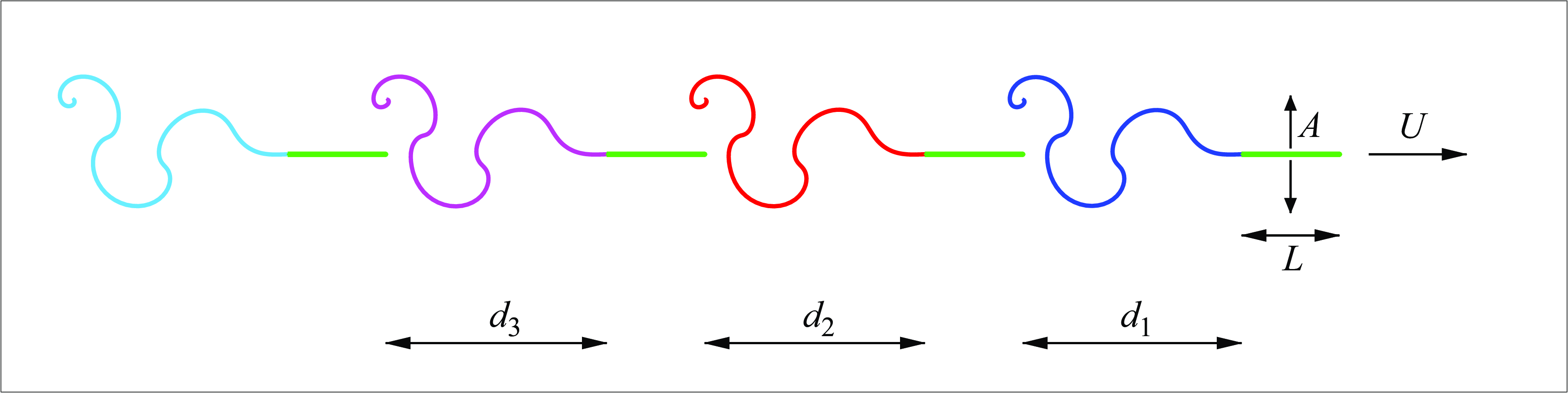
Figure 1. Schematic of the vortex sheet model. The plates (green), each of length $L$
, are in an in-line formation and heave periodically in the vertical direction with amplitude
$L$
, are in an in-line formation and heave periodically in the vertical direction with amplitude $A$
and frequency
$A$
and frequency $f$
while translating to the right with horizontal velocity
$f$
while translating to the right with horizontal velocity $U$
. The vortex sheet shed by the first, second, third or fourth plate is coloured blue, red, pink or cyan, respectively, a colour scheme that will be repeated throughout the text. The figure shows a sample simulation at
$U$
. The vortex sheet shed by the first, second, third or fourth plate is coloured blue, red, pink or cyan, respectively, a colour scheme that will be repeated throughout the text. The figure shows a sample simulation at $t=3.25$
(which equals 1.625 flapping periods) of
$t=3.25$
(which equals 1.625 flapping periods) of $n=4$
plates with
$n=4$
plates with $A = 0.1$
that were initially equispaced by a distance
$A = 0.1$
that were initially equispaced by a distance $d_0 = 2.25$
. The tail-to-tip distances
$d_0 = 2.25$
. The tail-to-tip distances $d_i$
are also shown.
$d_i$
are also shown.
The model used to simulate $n$
flapping plates is illustrated in figure 1, for
$n$
flapping plates is illustrated in figure 1, for $n=4$
. The fluid is assumed to be inviscid and incompressible, and also irrotational except for the wake behind each plate. The wake is modelled by a vortex sheet formed by shedding vorticity from the plates’ trailing edges at each time step. The plates are modelled by bound vortex sheets, with vortex sheet strength determined to satisfy the no-penetration boundary condition, or the requirement that no fluid flows through the plates. The fluid velocity in turn is determined by the vorticity in the plates and the wakes.
$n=4$
. The fluid is assumed to be inviscid and incompressible, and also irrotational except for the wake behind each plate. The wake is modelled by a vortex sheet formed by shedding vorticity from the plates’ trailing edges at each time step. The plates are modelled by bound vortex sheets, with vortex sheet strength determined to satisfy the no-penetration boundary condition, or the requirement that no fluid flows through the plates. The fluid velocity in turn is determined by the vorticity in the plates and the wakes.
The plates are all of length $L$
and mass per unit span
$L$
and mass per unit span $M$
, and are constrained to maintain an in-line formation, in that their cycle-averaged positions lie on a single horizontal line. They are initially separated by a distance
$M$
, and are constrained to maintain an in-line formation, in that their cycle-averaged positions lie on a single horizontal line. They are initially separated by a distance $d_0$
from their nearest neighbours, and are given the same initial horizontal velocity
$d_0$
from their nearest neighbours, and are given the same initial horizontal velocity $U_0$
. The prescribed vertical heaving motion is oscillatory with vertical position
$U_0$
. The prescribed vertical heaving motion is oscillatory with vertical position $A\sin (2\unicode{x03C0} f t)$
, corresponding to frequency
$A\sin (2\unicode{x03C0} f t)$
, corresponding to frequency $f$
and amplitude
$f$
and amplitude $A$
. This vertical motion induces a horizontal thrust that accelerates the plates, and is countered by a skin friction drag. Thrust and drag forces vary from plate to plate, causing distinct horizontal plate motion and thus distinct evolution of the separation distances
$A$
. This vertical motion induces a horizontal thrust that accelerates the plates, and is countered by a skin friction drag. Thrust and drag forces vary from plate to plate, causing distinct horizontal plate motion and thus distinct evolution of the separation distances $d_j(t)$
between the plates.
$d_j(t)$
between the plates.
While the flow is assumed to be inviscid, viscous effects are accounted for in two ways. First, they are necessary for vorticity to separate from the bodies. Second, they lead to a skin friction drag $F_{{d}}$
on each plate, which we model using the Blasius boundary layer drag law
$F_{{d}}$
on each plate, which we model using the Blasius boundary layer drag law $F_{{d}}=-C_{{d}}\rho\, \sqrt {L\nu }\,U^{3/2}$
, where
$F_{{d}}=-C_{{d}}\rho\, \sqrt {L\nu }\,U^{3/2}$
, where $C_{{d}}$
is the drag coefficient,
$C_{{d}}$
is the drag coefficient, $\nu$
is the fluid kinematic viscosity,
$\nu$
is the fluid kinematic viscosity, $\rho$
is the fluid density, and
$\rho$
is the fluid density, and $U$
is the instantaneous horizontal velocity of the plate. An alternative drag model used by Fang (Reference Fang2016) and Heydari & Kanso (Reference Heydari and Kanso2021) more closely accounts for the velocity above and below the plate. However, in Appendix C we present a comparison between these two models, which shows that the differences between them are minor. We thus opt to proceed with the simpler drag model herein. The resulting governing equations of the fluid flow and plates’ dynamics is non-dimensionalised by using the plate length
$U$
is the instantaneous horizontal velocity of the plate. An alternative drag model used by Fang (Reference Fang2016) and Heydari & Kanso (Reference Heydari and Kanso2021) more closely accounts for the velocity above and below the plate. However, in Appendix C we present a comparison between these two models, which shows that the differences between them are minor. We thus opt to proceed with the simpler drag model herein. The resulting governing equations of the fluid flow and plates’ dynamics is non-dimensionalised by using the plate length $L$
as the length scale, the flapping half-period
$L$
as the length scale, the flapping half-period $1/(2f)$
as the time scale, and
$1/(2f)$
as the time scale, and $4\rho (Lf)^2$
as the pressure scale. In this paper, we fix the values of the dimensionless plate mass
$4\rho (Lf)^2$
as the pressure scale. In this paper, we fix the values of the dimensionless plate mass $\tilde {M}=M/\rho L^2$
and drag coefficient
$\tilde {M}=M/\rho L^2$
and drag coefficient $\tilde {C}_{{d}}=C_{{d}}\sqrt {\nu /(2fL^2)}$
, as will be discussed in § 3.1, and study the dependence of the plate motion on the initial velocity
$\tilde {C}_{{d}}=C_{{d}}\sqrt {\nu /(2fL^2)}$
, as will be discussed in § 3.1, and study the dependence of the plate motion on the initial velocity $\tilde {U}_0=U_0/(2Lf)$
, the initial separation distance
$\tilde {U}_0=U_0/(2Lf)$
, the initial separation distance $\tilde {d}_0=d_0/L$
, the flapping amplitude
$\tilde {d}_0=d_0/L$
, the flapping amplitude $\tilde {A}=A/L$
, and the number of plates
$\tilde {A}=A/L$
, and the number of plates $n$
. From here on, all variables are non-dimensional and the tildes are dropped.
$n$
. From here on, all variables are non-dimensional and the tildes are dropped.
2.1. The vortex sheet model
The $n$
bound vortex sheets representing the flat plates have positions
$n$
bound vortex sheets representing the flat plates have positions
 \begin{equation} \boldsymbol{x}_b^j(\alpha,t)=(x_b^j,y_b^j)(\alpha,t),\quad \alpha \in [0,\unicode{x03C0}],\quad j=1,\ldots,n, \end{equation}
and sheet strengths $\gamma ^j(\alpha,t)$
. The sheets are initially on the horizontal
$\gamma ^j(\alpha,t)$
. The sheets are initially on the horizontal $x$
-axis, with position
$x$
-axis, with position
 \begin{align} x_b^j(\alpha,0)&=s(\alpha) - (j-1)(d_0+1),\quad s(\alpha)=\cos (\alpha)/2, \end{align}
 \begin{align} y_b^j(\alpha,0)&=0\,. \end{align}
That is, each plate has unit length, with $\alpha =0$
at the leading edge (right),
$\alpha =0$
at the leading edge (right), $\alpha =\unicode{x03C0}$
at the trailing edge (left), and
$\alpha =\unicode{x03C0}$
at the trailing edge (left), and $d_0$
the tail-to-tip distance between plates. The horizontal evolution of
$d_0$
the tail-to-tip distance between plates. The horizontal evolution of $x^j_b$
is determined by the displacement
$x^j_b$
is determined by the displacement $X^j(t)$
of plate
$X^j(t)$
of plate $j$
from its initial position, while the oscillatory vertical component
$j$
from its initial position, while the oscillatory vertical component $y^j_b(t)$
is prescribed:
$y^j_b(t)$
is prescribed:
 \begin{align} x^j_b(\alpha,t)&=X^j(t) + x_b^j(\alpha,0), \quad X^j(0)=0 \end{align}
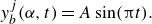 \begin{align} y^j_b(\alpha,t)&=A\sin (\unicode{x03C0} t). \end{align}
The plate position $X^j(t)$
evolves according to the induced thrust and drag forces acting on the plate (see § 2.2). The plate vortex sheet strength is determined numerically by enforcing the no-penetration boundary condition on the plate walls.
$X^j(t)$
evolves according to the induced thrust and drag forces acting on the plate (see § 2.2). The plate vortex sheet strength is determined numerically by enforcing the no-penetration boundary condition on the plate walls.
The free vortex sheets representing the wakes are parametrised by the circulation parameter $\Gamma$
, where
$\Gamma$
, where $\Gamma _T^j$
is the total circulation around the
$\Gamma _T^j$
is the total circulation around the $j$
th sheet:
$j$
th sheet:
 \begin{equation} \boldsymbol{x}_f^j(\Gamma,t),\quad \Gamma \in [0,\Gamma _T^j],\quad j=1,\ldots,n. \end{equation}
Together, the free and bound vortex sheets induce the fluid velocity at any point $\boldsymbol{x}_o$
:
$\boldsymbol{x}_o$
:
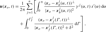 \begin{align} \notag\boldsymbol{u}(\boldsymbol{x}_o,t) &= \frac {1}{2\unicode{x03C0} }\sum _{j=1}^n \left [ \int _0^{\unicode{x03C0} } \frac { (\boldsymbol{x}_o-\boldsymbol{x}_b^j(\alpha,t))^{\perp } } {|\boldsymbol{x}_o-\boldsymbol{x}_b^j(\alpha,t)\vphantom{x_f}|^2}\,\gamma ^j(\alpha,t)\, s^{\prime}(\alpha)\,\mathrm{d}\alpha \right. \\ &\quad\left. +\int _0^{\Gamma _T^j} \frac { (\boldsymbol{x}_o-\boldsymbol{x}_f^j(\Gamma,t))^{\perp } } {|\boldsymbol{x}_o-\boldsymbol{x}_f^j(\Gamma,t)|^2+\delta ^2}\,\mathrm{d}\Gamma \right], \end{align}
where $(x,y)^{\perp }=(-y,x)$
. Here, the parameter
$(x,y)^{\perp }=(-y,x)$
. Here, the parameter $\delta$
regularises the flow for points
$\delta$
regularises the flow for points $\boldsymbol{x}_o$
near or on the free sheet, using the vortex blob method (Krasny Reference Krasny1986). If
$\boldsymbol{x}_o$
near or on the free sheet, using the vortex blob method (Krasny Reference Krasny1986). If $\boldsymbol{x}_o$
is a point on the plate, then the integrals in (2.6) are evaluated in the principal value sense, and yield the average of the velocity above and below the plate.
$\boldsymbol{x}_o$
is a point on the plate, then the integrals in (2.6) are evaluated in the principal value sense, and yield the average of the velocity above and below the plate.
The free sheet evolves with the fluid velocity (2.6) as
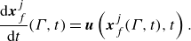 \begin{equation} \frac {\mathrm{d}\boldsymbol{x}_f^j}{\mathrm{d} t}(\Gamma,t) =\boldsymbol{u}\left (\boldsymbol{x}_f^j(\Gamma,t),t\right). \end{equation}
Its circulation $\Gamma$
is determined using the circulation shedding algorithm of Nitsche & Krasny (Reference Nitsche and Krasny1994). Vorticity is shed at time
$\Gamma$
is determined using the circulation shedding algorithm of Nitsche & Krasny (Reference Nitsche and Krasny1994). Vorticity is shed at time $t$
by releasing a particle from the plate’s trailing edge, with vertical velocity equal to the plate’s vertical velocity, and horizontal velocity equal to the average horizontal fluid velocity
$t$
by releasing a particle from the plate’s trailing edge, with vertical velocity equal to the plate’s vertical velocity, and horizontal velocity equal to the average horizontal fluid velocity $u(\boldsymbol{x}^j(\unicode{x03C0},t),t)=\overline {U}_e^j$
at the trailing edge, as obtained from (2.6). The particle’s circulation is such that the Kutta condition is satisfied, with
$u(\boldsymbol{x}^j(\unicode{x03C0},t),t)=\overline {U}_e^j$
at the trailing edge, as obtained from (2.6). The particle’s circulation is such that the Kutta condition is satisfied, with
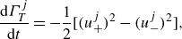 \begin{align} \frac {\mathrm{d}\Gamma _T^j}{\mathrm{d} t} &= -\frac {1}{2}[(u^j_+)^2-(u^j_-)^2], \end{align}
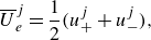 \begin{align} \overline {U}_e^j&=\frac {1}{2}(u^j_++u^j_-), \end{align}
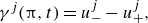 \begin{align} \gamma ^j(\unicode{x03C0},t)&=u_-^j - u_+^j, \end{align}
Here, $u^j_+$
and
$u^j_+$
and $u^j_-$
are the horizontal velocity components above and below the
$u^j_-$
are the horizontal velocity components above and below the $j$
th plate at the trailing edge, obtained from
$j$
th plate at the trailing edge, obtained from $\gamma ^j(\unicode{x03C0},t)$
and
$\gamma ^j(\unicode{x03C0},t)$
and $\overline {U}_e^j$
.
$\overline {U}_e^j$
.
2.2. Thrust and drag
The plates experience a thrust force due to the suction at their leading edges, which arises because the fluid velocity is singular there. Specifically, the thrust is obtained from the leading edge bound vortex sheet strength. The sheet strength is unbounded at the leading edge, with $\gamma ^j(\alpha,t)\sim \Delta s^{-1/2}$
as
$\gamma ^j(\alpha,t)\sim \Delta s^{-1/2}$
as $\Delta s\rightarrow 0$
, where
$\Delta s\rightarrow 0$
, where $\Delta s=1/2-s(\alpha)$
is the distance from the leading edge. However, the desingularised vortex sheet strength
$\Delta s=1/2-s(\alpha)$
is the distance from the leading edge. However, the desingularised vortex sheet strength $\gamma ^j(\alpha)\,s^{\prime}(\alpha)$
remains bounded. The horizontal thrust force acting on the plate is given by (Fang et al. Reference Fang, Ho, Ristroph and Shelley2017; Eldredge Reference Eldredge2019)
$\gamma ^j(\alpha)\,s^{\prime}(\alpha)$
remains bounded. The horizontal thrust force acting on the plate is given by (Fang et al. Reference Fang, Ho, Ristroph and Shelley2017; Eldredge Reference Eldredge2019)
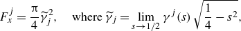 \begin{equation} F^j_x=\frac {\unicode{x03C0} }{4}\widetilde {\gamma }_j^2, \quad \text{where } \widetilde {\gamma }_j=\lim \limits _{s\to 1/2}\gamma ^j(s)\,\sqrt {\frac {1}{4}-s^2}, \end{equation}
and, with our choice of $s(\alpha)=\cos \alpha /2$
,
$s(\alpha)=\cos \alpha /2$
,
 \begin{equation} \widetilde {\gamma }_j=-\lim \limits _{\alpha \to 0}\gamma ^j(\alpha)\,s^{\prime}(\alpha). \end{equation}
The relation (2.9) holds for steady or unsteady plate motion. For steady motions, the result reduces to $\widetilde {\gamma }=-2V$
, where
$\widetilde {\gamma }=-2V$
, where $V$
is the vertical velocity of the leading edge, which is used by Alben (Reference Alben2010). For completeness, both the unsteady and steady results are derived here, in Appendices A and B, respectively. Appendix B also shows a comparison between the flow field around a plate in a steady vertical flow, and the unsteady flow field around an impulsively started plate moving vertically upwards with constant velocity, the latter being computed using the method described in § 2.3. We detail how the flow field (figure 14) and circulation (figure 15) in the unsteady case approach that of the steady case in the long-time limit.
$V$
is the vertical velocity of the leading edge, which is used by Alben (Reference Alben2010). For completeness, both the unsteady and steady results are derived here, in Appendices A and B, respectively. Appendix B also shows a comparison between the flow field around a plate in a steady vertical flow, and the unsteady flow field around an impulsively started plate moving vertically upwards with constant velocity, the latter being computed using the method described in § 2.3. We detail how the flow field (figure 14) and circulation (figure 15) in the unsteady case approach that of the steady case in the long-time limit.
As discussed at the beginning of § 2, the drag force acting on the plate is modelled to be proportional to $(U^j(t))^{3/2}$
, where
$(U^j(t))^{3/2}$
, where $U^j(t)$
is the plate velocity. The horizontal motion of the
$U^j(t)$
is the plate velocity. The horizontal motion of the $n$
plates is thus governed by the system of ordinary differential equations
$n$
plates is thus governed by the system of ordinary differential equations
 \begin{align} \frac {\mathrm{d} X^j}{\mathrm{d} t}&= U^j, \quad X^j(0)=0 \end{align}
 \begin{align} M\frac {\mathrm{d} U^j}{\mathrm{d} t}&=\frac {\unicode{x03C0} }{4}\widetilde {\gamma }_j^2-C_{{d}} (U^j)^{3/2},\quad U^j(0)=U_0. \end{align}
The flow evolution is determined by the system of ordinary differential equations (ODEs) (2.7), (2.8) and (2.11), in addition to a Fredholm integral equation for $\widetilde {\gamma }$
. Its numerical solution is described next.
$\widetilde {\gamma }$
. Its numerical solution is described next.
2.3. Numerical method
The plates (2.1) are each discretised by $N_b+1$
point vortices corresponding to
$N_b+1$
point vortices corresponding to $\alpha _k=k\unicode{x03C0} /N_b$
,
$\alpha _k=k\unicode{x03C0} /N_b$
, $k=0,\ldots,N_b$
. The free vortex sheets are discretised by
$k=0,\ldots,N_b$
. The free vortex sheets are discretised by $N_f+1$
vortex blobs with total circulation
$N_f+1$
vortex blobs with total circulation $\Gamma _T^j$
, created by shedding one blob at each time step; thus
$\Gamma _T^j$
, created by shedding one blob at each time step; thus $N_f$
increases with time. Time is discretised by
$N_f$
increases with time. Time is discretised by $t_m=m\,\Delta t(t)$
, where typically
$t_m=m\,\Delta t(t)$
, where typically $\Delta t$
is smaller at early times near the beginning of the motion, and increases linearly from
$\Delta t$
is smaller at early times near the beginning of the motion, and increases linearly from $\Delta t_1$
to a final time step
$\Delta t_1$
to a final time step $\Delta t_2$
at a time
$\Delta t_2$
at a time $t_1$
, after which it remains constant. The small initial time steps are needed to resolve the large initial velocities about the trailing edge. The system of ODEs (2.7), (2.8) and (2.11) is solved using the fourth-order Runge–Kutta method. At each stage, the following steps are taken (Sheng et al. Reference Sheng, Ysasi, Kolomenskiy, Kanso, Nitsche, Schneider, Childress, Hosoi, Schultz and Wang2012).
$t_1$
, after which it remains constant. The small initial time steps are needed to resolve the large initial velocities about the trailing edge. The system of ODEs (2.7), (2.8) and (2.11) is solved using the fourth-order Runge–Kutta method. At each stage, the following steps are taken (Sheng et al. Reference Sheng, Ysasi, Kolomenskiy, Kanso, Nitsche, Schneider, Childress, Hosoi, Schultz and Wang2012).
-
(i) Set the vertical plate velocity $V(t)=A\unicode{x03C0} \cos (\unicode{x03C0} t)$
.
$V(t)=A\unicode{x03C0} \cos (\unicode{x03C0} t)$
. -
(ii) For each plate
$j=1,\ldots,n$
, find the sheet strength
$\gamma ^j_k=\gamma ^j(\alpha _k,t)$
such that the vertical fluid velocity in (2.6) evaluated at the midpoints
$\alpha _k^m=(\alpha _{k-1}+\alpha _k)/2$
equals the prescribed vertical plate velocity,(2.12)where
\begin{equation} \boldsymbol{u}\left (\boldsymbol{x}^j_b(\alpha ^m_k,t),t\right)\boldsymbol{\cdot} \boldsymbol{n} = V(t),\quad k=1,\ldots,N_b, \end{equation}
$\boldsymbol{n}=(0,1)$
is normal to the plate. Here, the singular integrals in the velocity (2.6) are computed with what is in essence the alternating point vortex method of Shelley (Reference Shelley1992). In addition, enforce zero total circulation around the plate and its wake. The resulting
$(N_b+1)\times (N_b+1)$
linear system for
$\gamma ^j_k$
,
$k=0, \ldots, N_b$
, is inverted using a precomputed LU decomposition.
-
(iii) Set
$\gamma ^j(\unicode{x03C0},t)= \gamma ^j_{N_b}$
and
$\overline {U}_e^j= u (\boldsymbol{x}_b^j (\alpha _{N_b}^m,t),t)$
, and obtain
$u_j^+$
and
$u_j^-$
using (2.8b
) and (2.8c
). Then shed a particle
$\boldsymbol{x}^j_{{new}}$
from each trailing edge with velocity(2.13)and circulation such that (2.8a ) is satisfied. As explained by Nitsche & Krasny (Reference Nitsche and Krasny1994, § 2.4(iii)), only separated flow is considered when determining
\begin{equation} \frac {\mathrm{d} \boldsymbol{x}^j_{{new}}}{\mathrm{d} t}= (\overline {U}_e^j,V) \end{equation}
$u_j^+$
and
$u_j^-$
.
-
(iv) Move all previously shed particles with velocity
(2.14)and add
\begin{equation} \frac {\mathrm{d} \boldsymbol{x}^j_{f,k}}{\mathrm{d} t}= \boldsymbol{u}\left (\boldsymbol{x}^j_{f,k},t\right),\quad k=0,\ldots,N^j_f, \end{equation}
$\boldsymbol{x}^j_{f,N^j_f+1}=\boldsymbol{x}^j_{{new}}$
, then increase
$N^j_f$
by 1. Here, the integral over the bound vortex sheets in (2.6) is near-singular when the target point is near a plate. The near-singular integrals are computed using the corrected trapezoid rule of Nitsche (Reference Nitsche2021).
-
(v) Determine the desingularised leading edge sheet strength
$\widetilde {\gamma }_j$
using (2.10), and move the plates by (2.11).


Typically, one new particle is shed per time step. In some cases, a particle is shed every other time step or more for the sake of computational efficiency.
3. Numerical results
This section presents numerical results for $n=1$
, 2, 3 and 4 plates, with flapping amplitudes
$n=1$
, 2, 3 and 4 plates, with flapping amplitudes $A=0.1{-}0.4$
, mass
$A=0.1{-}0.4$
, mass $M=1$
, and drag coefficient
$M=1$
, and drag coefficient $C_{{d}}=0.1$
. The numerical parameters are
$C_{{d}}=0.1$
. The numerical parameters are $\delta =0.2$
,
$\delta =0.2$
, $N_b=100$
,
$N_b=100$
, $t_1=1$
,
$t_1=1$
, $\Delta t_2=0.008/A$
and
$\Delta t_2=0.008/A$
and $\Delta t_1\approx \Delta t_2/10$
. Results were confirmed to remain basically unchanged under mesh refinement (decreasing
$\Delta t_1\approx \Delta t_2/10$
. Results were confirmed to remain basically unchanged under mesh refinement (decreasing $\Delta t$
, increasing
$\Delta t$
, increasing $N_b$
) or smaller values of
$N_b$
) or smaller values of $\delta$
.
$\delta$
.
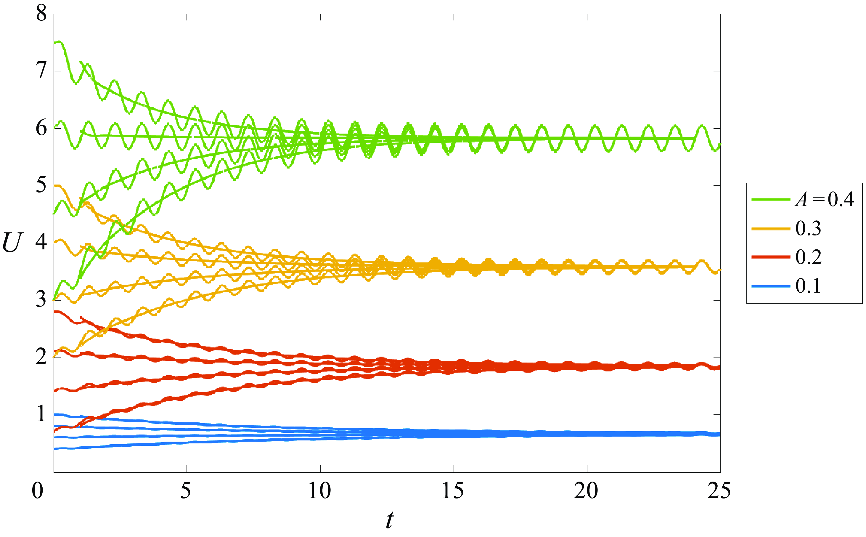
Figure 2. Time evolution of the translation velocity $U$
of a single plate (
$U$
of a single plate ( $n=1$
), for various initial velocities
$n=1$
), for various initial velocities $U_0$
and the four amplitudes
$U_0$
and the four amplitudes $A$
indicated in the legend. The oscillatory curves show the instantaneous velocity
$A$
indicated in the legend. The oscillatory curves show the instantaneous velocity $U(t)$
, upon which we have superimposed a cycle-averaged velocity obtained by averaging
$U(t)$
, upon which we have superimposed a cycle-averaged velocity obtained by averaging $U(t)$
over a moving window of size equal to the oscillation period.
$U(t)$
over a moving window of size equal to the oscillation period.
3.1.
Single plate,
$n=1$

Here, we consider one plate moving with a prescribed oscillatory heaving motion of amplitude $A$
, given an initial horizontal velocity
$A$
, given an initial horizontal velocity $U_0$
. The plate moves forward by the thrust force (2.9), as vorticity is shed from its trailing edge. Figure 2 shows the resulting horizontal plate velocity for a range of amplitudes
$U_0$
. The plate moves forward by the thrust force (2.9), as vorticity is shed from its trailing edge. Figure 2 shows the resulting horizontal plate velocity for a range of amplitudes $A$
and initial velocities
$A$
and initial velocities $U_0$
. The plate horizontal velocity oscillates with the same frequency as the heaving motion. For each case, the figure shows both the actual oscillatory velocity
$U_0$
. The plate horizontal velocity oscillates with the same frequency as the heaving motion. For each case, the figure shows both the actual oscillatory velocity $U(t)$
, and the cycle-averaged velocity obtained by averaging
$U(t)$
, and the cycle-averaged velocity obtained by averaging $U(t)$
over a moving window of size equal to the oscillation period. The figure shows that in all cases, the cycle-averaged plate velocity approaches a steady-state velocity
$U(t)$
over a moving window of size equal to the oscillation period. The figure shows that in all cases, the cycle-averaged plate velocity approaches a steady-state velocity $U_{\infty }$
that depends solely on the amplitude
$U_{\infty }$
that depends solely on the amplitude $A$
and is independent of the initial velocity
$A$
and is independent of the initial velocity $U_0$
. The steady-state velocity
$U_0$
. The steady-state velocity $U_{\infty }$
increases as
$U_{\infty }$
increases as $A$
increases, with values
$A$
increases, with values $U_{\infty }=0.665$
, 1.85, 3.58 and 5.83 for
$U_{\infty }=0.665$
, 1.85, 3.58 and 5.83 for $A=0.1$
, 0.2, 0.3 and 0.4, respectively. These values of
$A=0.1$
, 0.2, 0.3 and 0.4, respectively. These values of $U_{\infty }$
are approximately consistent with those obtained in experiments on heaving wings in a water tank (Ramananarivo et al. Reference Ramananarivo, Fang, Oza, Zhang and Ristroph2016), which motivates our choice of the drag coefficient
$U_{\infty }$
are approximately consistent with those obtained in experiments on heaving wings in a water tank (Ramananarivo et al. Reference Ramananarivo, Fang, Oza, Zhang and Ristroph2016), which motivates our choice of the drag coefficient $C_{{d}}$
.
$C_{{d}}$
.
Figure 3(a) shows the shed vortex sheet behind one plate oscillating with amplitude $A=0.2$
, at time
$A=0.2$
, at time $t=25$
. The given initial velocity is that of the corresponding steady state,
$t=25$
. The given initial velocity is that of the corresponding steady state, $U_0=1.85$
. With each upward (downward) motion of the plate, positive (negative) vorticity is shed from the trailing edge, which leads to a sequence of counter-rotating vortex pairs shed during each oscillation period. By taking the curl of (2.6), we obtain the regularised vorticity corresponding to the shed vortex sheet, which is shown in figure 4(a). Soon after being shed, the vorticity settles into a sequence of almost equally spaced vortices of alternating sign, with the positive (negative) vortex positioned slightly below (above) the centreline
$U_0=1.85$
. With each upward (downward) motion of the plate, positive (negative) vorticity is shed from the trailing edge, which leads to a sequence of counter-rotating vortex pairs shed during each oscillation period. By taking the curl of (2.6), we obtain the regularised vorticity corresponding to the shed vortex sheet, which is shown in figure 4(a). Soon after being shed, the vorticity settles into a sequence of almost equally spaced vortices of alternating sign, with the positive (negative) vortex positioned slightly below (above) the centreline $y=0$
.
$y=0$
.
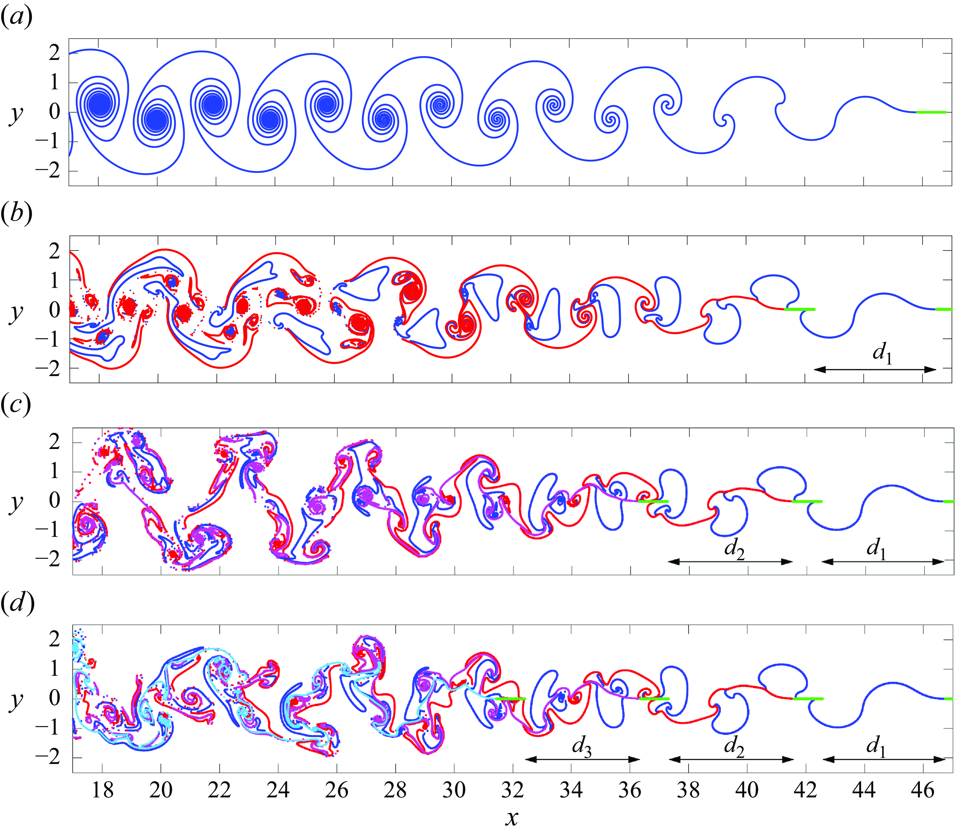
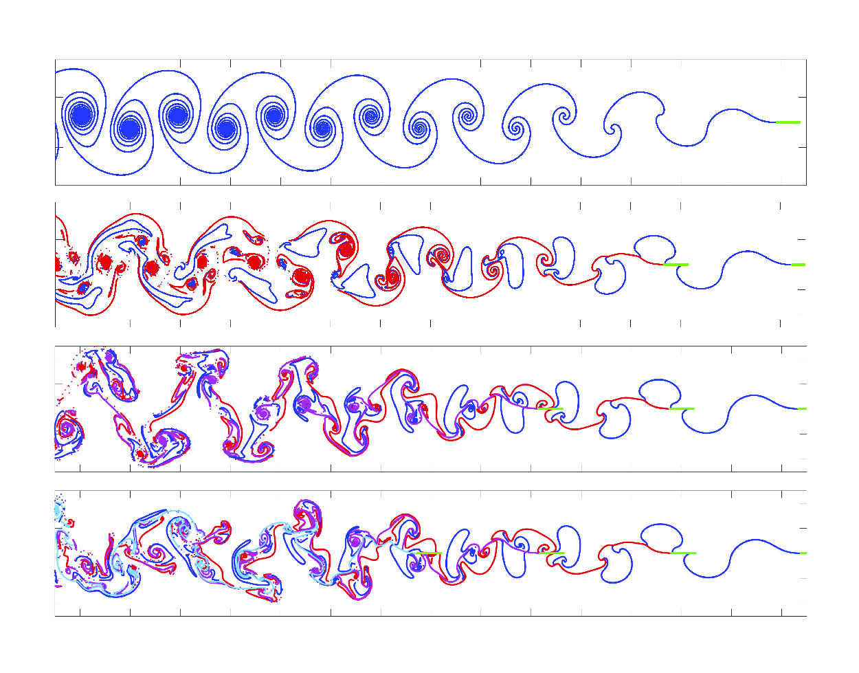
Figure 3. Plate and vortex sheet positions at $t=25$
, for the flapping amplitude
$t=25$
, for the flapping amplitude $A=0.2$
and
$A=0.2$
and $n=1$
, 2, 3 and 4 plates (from top to bottom). All plates are initially equispaced with a distance near
$n=1$
, 2, 3 and 4 plates (from top to bottom). All plates are initially equispaced with a distance near $d_0=4.2$
.
$d_0=4.2$
.
3.2.
Several plates,
$n=2,3,4$

Figure 3(b) shows the two vortex sheets shed behind two plates, both heaving with amplitude $A=0.2$
. The colour scheme is the same as that in figure 1, with the vortex sheet shed by the leader (follower) plate indicated in blue (red). There is a large amount of stretching far downstream of the plates as the two sheets interact. We plot the sheets using a linear interpolant of the shed point vortices if neighbouring points are sufficiently close to each other. Otherwise, after a sufficiently large amount of stretching, we simply plot the individual point vortex positions. The initial distance between the plates is
$A=0.2$
. The colour scheme is the same as that in figure 1, with the vortex sheet shed by the leader (follower) plate indicated in blue (red). There is a large amount of stretching far downstream of the plates as the two sheets interact. We plot the sheets using a linear interpolant of the shed point vortices if neighbouring points are sufficiently close to each other. Otherwise, after a sufficiently large amount of stretching, we simply plot the individual point vortex positions. The initial distance between the plates is $d_0=4.2$
, which is, as will be seen later, near an equilibrium position. The two sheets are seen to roll up into four vortices per period, a phenomenon that is also evident in the top panel of supplementary movie 1. This is seen more clearly in figure 4(b), which shows a sequence of two positive vortices followed by two negative vortices per period. This pattern repeats, although in an irregular fashion. Groups of four vortices are discernible, but their relative positions do not settle into a clear steady pattern.
$d_0=4.2$
, which is, as will be seen later, near an equilibrium position. The two sheets are seen to roll up into four vortices per period, a phenomenon that is also evident in the top panel of supplementary movie 1. This is seen more clearly in figure 4(b), which shows a sequence of two positive vortices followed by two negative vortices per period. This pattern repeats, although in an irregular fashion. Groups of four vortices are discernible, but their relative positions do not settle into a clear steady pattern.
Figure 3(c) shows the three vortex sheets shed behind three plates heaving with amplitude $A=0.2$
. The initial separation between all plates is as before,
$A=0.2$
. The initial separation between all plates is as before, $d_0=4.2$
. A pattern seems to appear farther downstream of the plates. Most notably, near
$d_0=4.2$
. A pattern seems to appear farther downstream of the plates. Most notably, near $x=20$
, the vortices have spread further from the midline
$x=20$
, the vortices have spread further from the midline $y=0$
. Figure 4(c) reveals more clearly a repeating pattern of groups of six vortices, i.e. three positive followed by three negative. Sufficiently far downstream, for
$y=0$
. Figure 4(c) reveals more clearly a repeating pattern of groups of six vortices, i.e. three positive followed by three negative. Sufficiently far downstream, for $x\lt 25$
, the vorticity is clearly concentrated away from the midline, as it has spread significantly farther than in the
$x\lt 25$
, the vorticity is clearly concentrated away from the midline, as it has spread significantly farther than in the $n=2$
case shown in figure 4(b). A simulation with
$n=2$
case shown in figure 4(b). A simulation with $n=3$
plates is shown in supplementary movie 2.
$n=3$
plates is shown in supplementary movie 2.
Figures 3(d) and 4(d) show the vortex sheets and corresponding vorticity shed behind $n=4$
moving plates. It is difficult to detect a pattern in the downstream vortex sheet positions. The vorticity is expected to consist of groups of eight vortices, i.e. four positive followed by four negative, but the pattern is less clear and more random. Furthermore, the spread away from the midline is not as big as for
$n=4$
moving plates. It is difficult to detect a pattern in the downstream vortex sheet positions. The vorticity is expected to consist of groups of eight vortices, i.e. four positive followed by four negative, but the pattern is less clear and more random. Furthermore, the spread away from the midline is not as big as for $n=3$
. A simulation with
$n=3$
. A simulation with $n=4$
plates is shown in supplementary movie 3.
$n=4$
plates is shown in supplementary movie 3.
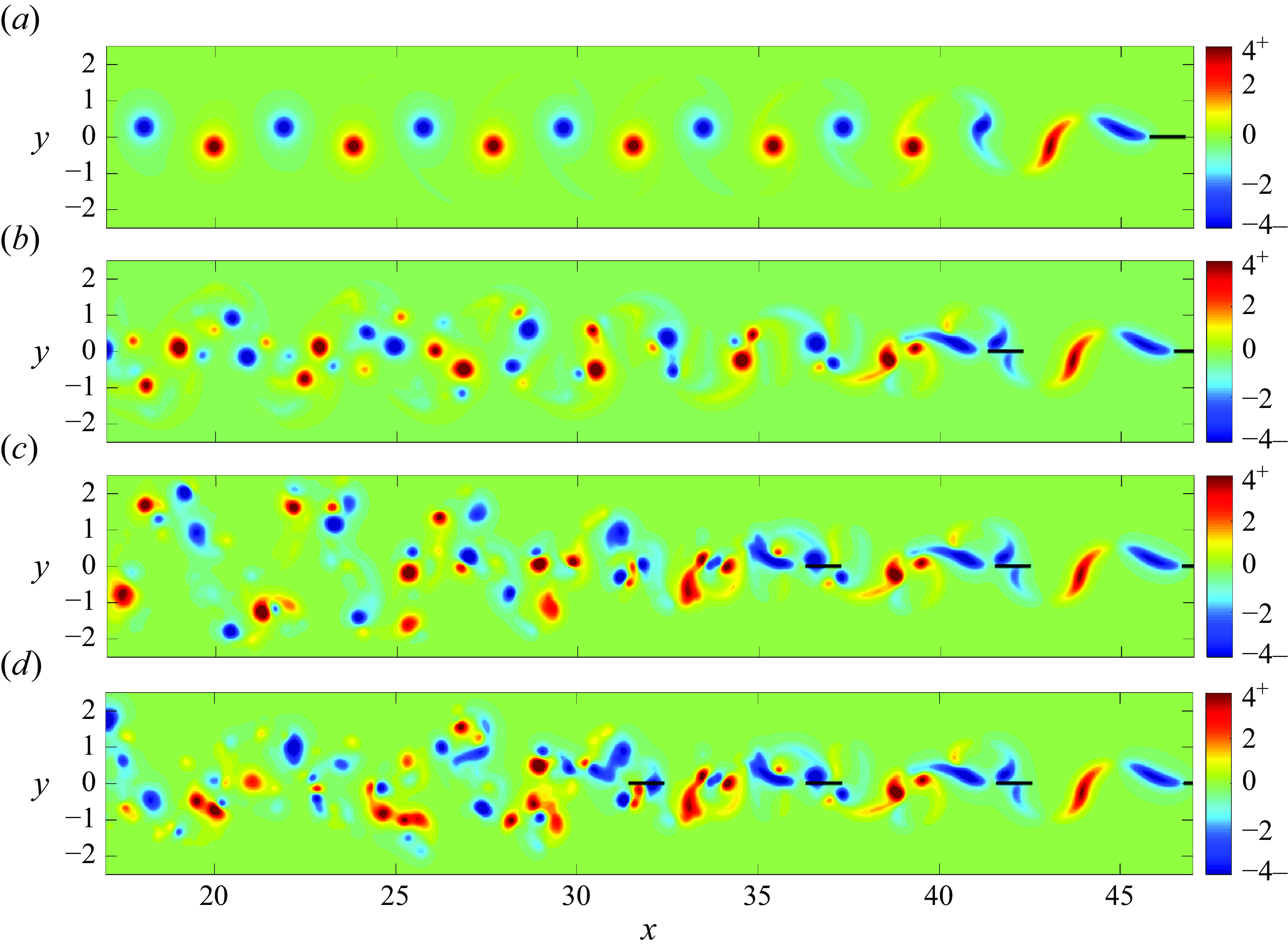
Figure 4. Same as figure 3, but the regularised vorticity is plotted instead of the vortex sheet. The plates are indicated in black. Absolute vorticity values larger than 4 are represented by the darkest blue and red colours.
The effect of the trailing plates on the leader is seen most clearly in figure 3. In all four cases, the given initial velocity is $U_0=1.85$
, and the initial distances between the plates are
$U_0=1.85$
, and the initial distances between the plates are $d_j(0)= 4.2$
. The shape of the sheet between the first and second plates is basically unchanged in all cases from the single-plate case. That is, the second plate has little influence on the wake in front of it. Similarly, the wake behind the second and third plates is unchanged from the
$d_j(0)= 4.2$
. The shape of the sheet between the first and second plates is basically unchanged in all cases from the single-plate case. That is, the second plate has little influence on the wake in front of it. Similarly, the wake behind the second and third plates is unchanged from the $n=2$
case, so the third plate also has little influence on the wake in front of it. It is evident that as the number of plates behind the front plate increases, the front plate has travelled slightly further by
$n=2$
case, so the third plate also has little influence on the wake in front of it. It is evident that as the number of plates behind the front plate increases, the front plate has travelled slightly further by $t=25$
. However, after an initial transient, we observe that
$t=25$
. However, after an initial transient, we observe that $U_{\infty }$
remains essentially unchanged, with only a small increase of less than 3 % as
$U_{\infty }$
remains essentially unchanged, with only a small increase of less than 3 % as $n$
increases. We attribute this increase in the leader’s velocity, albeit small, to the fact that the leader’s bound vorticity is modified by the downstream plates’ bound and shed vorticity, as is evident from step (ii) of the numerical method presented in § 2.3. The leader’s bound vorticity in turn affects its thrust, as given by (2.9).
$n$
increases. We attribute this increase in the leader’s velocity, albeit small, to the fact that the leader’s bound vorticity is modified by the downstream plates’ bound and shed vorticity, as is evident from step (ii) of the numerical method presented in § 2.3. The leader’s bound vorticity in turn affects its thrust, as given by (2.9).
3.3.
Steady-state positions for
$A=0.2$
,
$n=2$


The distances $d_j(t)$
between the plates evolve in time. We are interested in the long-term behaviour of
$d_j(t)$
between the plates evolve in time. We are interested in the long-term behaviour of $d_j$
and the associated possible steady-state configurations. This subsection presents results for a pair of wings (
$d_j$
and the associated possible steady-state configurations. This subsection presents results for a pair of wings ( $n=2$
) with flapping amplitude
$n=2$
) with flapping amplitude $A=0.2$
, with a range of initial separation distances
$A=0.2$
, with a range of initial separation distances $d_0$
. Since the steady-state cycle-averaged plate velocity
$d_0$
. Since the steady-state cycle-averaged plate velocity $U_{\infty }$
is found to always be independent of
$U_{\infty }$
is found to always be independent of $U_0$
, from here on, the initial horizontal velocity of each plate is taken to be the steady-state cycle-averaged velocity of a single plate flapping with the same amplitude. We observe that the two plates evolve towards a steady configuration in which the distance between them, after undergoing several oscillations, approaches a constant, but that this equilibrium distance
$U_0$
, from here on, the initial horizontal velocity of each plate is taken to be the steady-state cycle-averaged velocity of a single plate flapping with the same amplitude. We observe that the two plates evolve towards a steady configuration in which the distance between them, after undergoing several oscillations, approaches a constant, but that this equilibrium distance $d_1^{\infty }$
depends on the initial distance
$d_1^{\infty }$
depends on the initial distance $d_0$
. Figure 5 shows snapshots of simulations performed for three different values of
$d_0$
. Figure 5 shows snapshots of simulations performed for three different values of $d_0$
, at a time when the separation distance
$d_0$
, at a time when the separation distance $d_1$
between the plates has reached the equilibrium values
$d_1$
between the plates has reached the equilibrium values $d_1^{\infty,1}$
,
$d_1^{\infty,1}$
, $d_1^{\infty,2}$
and
$d_1^{\infty,2}$
and $d_1^{\infty,3}$
. Supplementary movie 1 also shows examples of simulations performed for different values of
$d_1^{\infty,3}$
. Supplementary movie 1 also shows examples of simulations performed for different values of $d_0$
, which illustrates how changing
$d_0$
, which illustrates how changing $d_0$
causes the pair of plates to attain different equilibria.
$d_0$
causes the pair of plates to attain different equilibria.
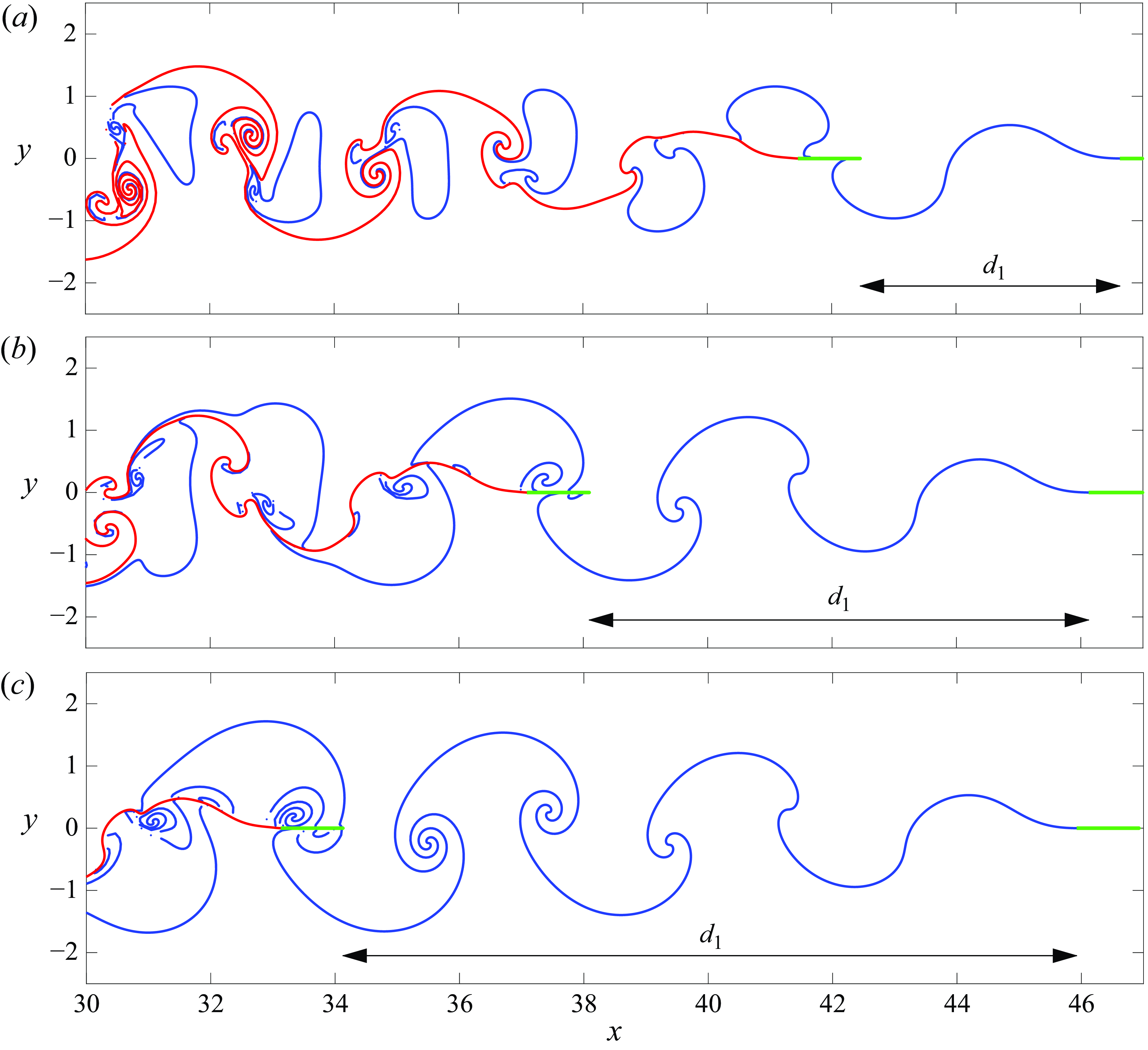
Figure 5. Snapshot at $t=25$
of three of the schooling modes obtained for a pair of plates (
$t=25$
of three of the schooling modes obtained for a pair of plates ( $n=2$
) with flapping amplitude
$n=2$
) with flapping amplitude $A = 0.2$
. The plates are initially located near the first, second and third equilibria, which, from top to bottom, correspond to the distances
$A = 0.2$
. The plates are initially located near the first, second and third equilibria, which, from top to bottom, correspond to the distances $d^{\infty,1}_1=4.18$
,
$d^{\infty,1}_1=4.18$
, $d^{\infty,2}_1=8.01$
and
$d^{\infty,2}_1=8.01$
and $d^{\infty,3}_1=11.82$
, respectively.
$d^{\infty,3}_1=11.82$
, respectively.
Note that in figure 5(a), the distance $d_1^{\infty,1}$
between the plates is approximately the distance travelled by the plate in one period of the heaving oscillation, as evident by the single upward and downward wave of the shed sheet. In figure 5(b), the equilibrium distance is approximately twice that of figure 5(a), and in figure 5(c) it is approximately three times. The distance travelled by a plate with velocity
$d_1^{\infty,1}$
between the plates is approximately the distance travelled by the plate in one period of the heaving oscillation, as evident by the single upward and downward wave of the shed sheet. In figure 5(b), the equilibrium distance is approximately twice that of figure 5(a), and in figure 5(c) it is approximately three times. The distance travelled by a plate with velocity $U_{\infty }$
in one oscillation period is the wavelength
$U_{\infty }$
in one oscillation period is the wavelength $\lambda =U_{\infty }/f$
, where
$\lambda =U_{\infty }/f$
, where $f=1/2$
. Using the value
$f=1/2$
. Using the value $U_{\infty }=1.85$
corresponding to
$U_{\infty }=1.85$
corresponding to $A=0.2$
, we find that the equilibrium positions satisfy
$A=0.2$
, we find that the equilibrium positions satisfy
 \begin{align} d^{\infty,1}_{1}\approx 4.18\approx 1.13\lambda,\quad d^{\infty,2}_{1}\approx 8.01 \approx 2.16\lambda \quad \text{and}\quad d^{\infty,3}_{1}\approx 11.82 \approx 3.19\lambda. \end{align}
Clearly, the plates have settled at equilibrium configurations near integer values of the non-dimensional schooling number (Becker et al. Reference Becker, Masoud, Newbolt, Shelley and Ristroph2015)
 \begin{equation} S_k=\frac {d^{\infty,k}_{1}}{\lambda }. \end{equation}
Note that while the first equilibrium has schooling number $S_{1}=1.13$
, i.e. slightly larger than 1, the following schooling numbers
$S_{1}=1.13$
, i.e. slightly larger than 1, the following schooling numbers $S_2=2.16$
and
$S_2=2.16$
and $S_3=3.19$
increase approximately by integer values,
$S_3=3.19$
increase approximately by integer values, $S_k\approx S_{k-1}+1$
.
$S_k\approx S_{k-1}+1$
.
3.4. Equilibrium schooling states and their loss of stability
Figure 6 shows the dependence of the distances $d_j(t)$
between plates on the initial separation distance
$d_j(t)$
between plates on the initial separation distance $d_0$
, for in-line formations of
$d_0$
, for in-line formations of $n=2$
, 3 and 4 wings (columns from left to right) and the three flapping amplitudes
$n=2$
, 3 and 4 wings (columns from left to right) and the three flapping amplitudes $A = 0.4$
, 0.3 and 0.1 (top to bottom rows). These flapping amplitudes complement the value
$A = 0.4$
, 0.3 and 0.1 (top to bottom rows). These flapping amplitudes complement the value $A=0.2$
considered in § 3.3. We proceed by discussing each column in turn.
$A=0.2$
considered in § 3.3. We proceed by discussing each column in turn.
The first column shows results for $n=2$
plates. It shows the distance
$n=2$
plates. It shows the distance $d_1(t)$
between the plates as a function of time, for 35 or 36 different initial separation distances
$d_1(t)$
between the plates as a function of time, for 35 or 36 different initial separation distances $d_0$
. During an initial time interval of length approximately
$d_0$
. During an initial time interval of length approximately $d_0/U_{\infty }$
, the vorticity of the leader has not yet reached the follower, and both plates travel with the same velocity, each without the influence of the other. During that time interval, the distance between them stays constant. The larger the initial distance
$d_0/U_{\infty }$
, the vorticity of the leader has not yet reached the follower, and both plates travel with the same velocity, each without the influence of the other. During that time interval, the distance between them stays constant. The larger the initial distance $d_0$
, the longer this initial time interval. Once the vortex wake of the leader reaches the follower, that vorticity changes the evolution of the follower, and the distance between the plates changes. In all cases, the distance
$d_0$
, the longer this initial time interval. Once the vortex wake of the leader reaches the follower, that vorticity changes the evolution of the follower, and the distance between the plates changes. In all cases, the distance $d_1(t)$
initially oscillates, then the amplitude of these oscillations decreases in time as
$d_1(t)$
initially oscillates, then the amplitude of these oscillations decreases in time as $d_1$
approaches a constant steady-state value. Notice that the steady-state distances
$d_1$
approaches a constant steady-state value. Notice that the steady-state distances $d_1^{\infty,k}$
decrease in proportion to
$d_1^{\infty,k}$
decrease in proportion to $U_{\infty }$
as
$U_{\infty }$
as $A$
decreases from 0.4 (top row) to 0.1 (bottom row). That is, as the heaving amplitude is decreased progressively, the plates are closer together in their steady configurations. Note also that the oscillations in
$A$
decreases from 0.4 (top row) to 0.1 (bottom row). That is, as the heaving amplitude is decreased progressively, the plates are closer together in their steady configurations. Note also that the oscillations in $d_1$
are larger, relative to the value of
$d_1$
are larger, relative to the value of $d_1$
, for smaller values of
$d_1$
, for smaller values of $A$
.
$A$
.
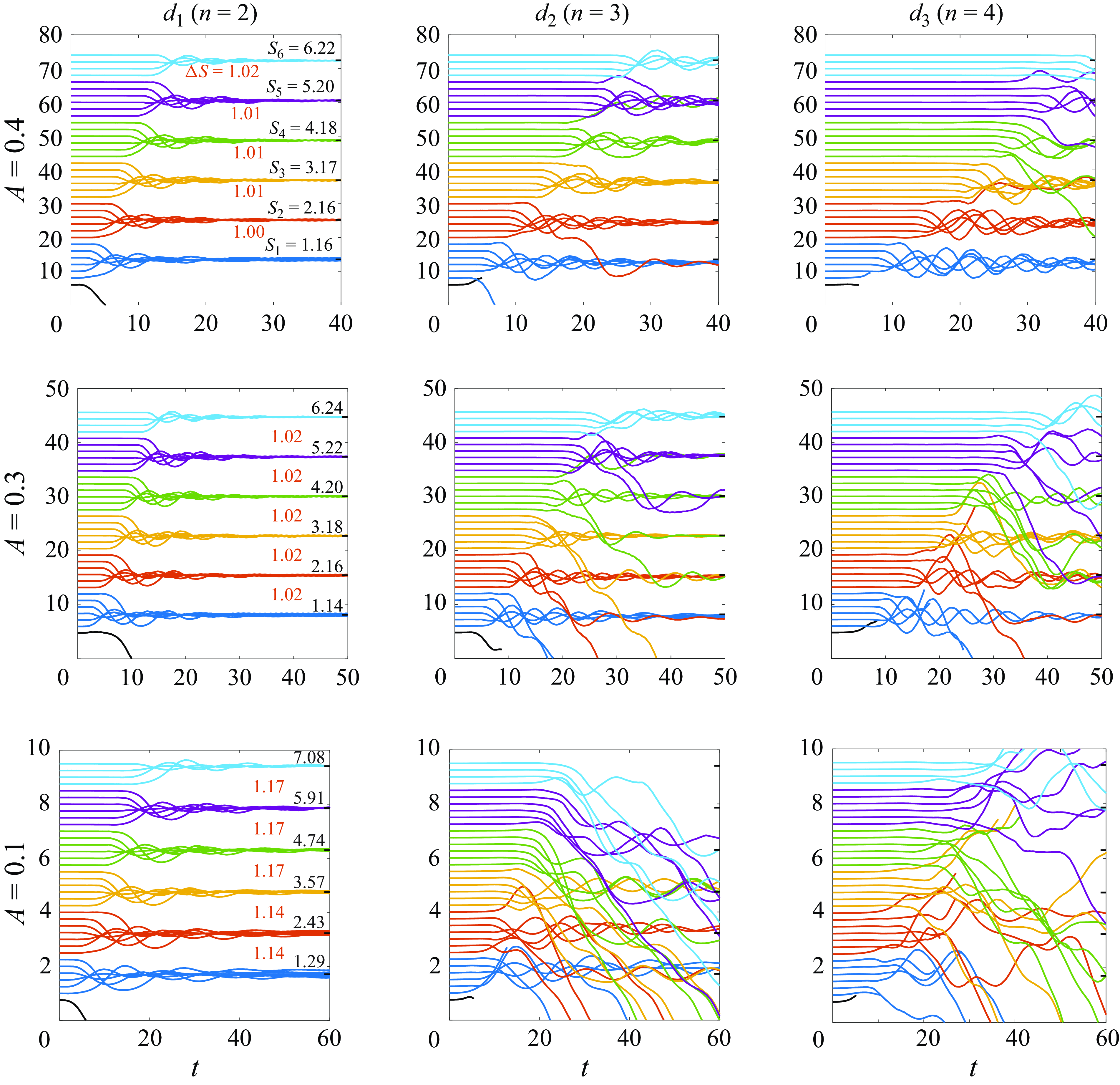
Figure 6. Time evolution of the distances $d_1(t)$
(left-hand column),
$d_1(t)$
(left-hand column), $d_2(t)$
(middle column) and
$d_2(t)$
(middle column) and $d_3(t)$
(right-hand column) for in-line formations of
$d_3(t)$
(right-hand column) for in-line formations of $n=2$
, 3 and 4 plates, respectively. The plots in the top, middle and bottom rows correspond to the heaving amplitudes
$n=2$
, 3 and 4 plates, respectively. The plots in the top, middle and bottom rows correspond to the heaving amplitudes $A = 0.4$
, 0.3 and 0.1, respectively. The different curves in each plot are obtained by varying the initial distances
$A = 0.4$
, 0.3 and 0.1, respectively. The different curves in each plot are obtained by varying the initial distances $d_j(0)$
, and are colour-coded according to the equilibrium schooling mode reached for two plates (
$d_j(0)$
, and are colour-coded according to the equilibrium schooling mode reached for two plates ( $n=2$
, left-hand column). The schooling numbers
$n=2$
, left-hand column). The schooling numbers $S_k=d^{\infty,k}_1/\lambda$
corresponding to each equilibrium distance
$S_k=d^{\infty,k}_1/\lambda$
corresponding to each equilibrium distance $d^{\infty,k}_1$
are written in black in the first column, with the differences between them written in red. Here,
$d^{\infty,k}_1$
are written in black in the first column, with the differences between them written in red. Here, $\lambda = 2U_{\infty }$
is computed using the steady-state
$\lambda = 2U_{\infty }$
is computed using the steady-state $U_{\infty }$
for the pair of plates.
$U_{\infty }$
for the pair of plates.
As already observed in figure 5, there are several steady states, depending on the value of $d_0$
. The steady states are measured by their schooling number (3.2), using the value for
$d_0$
. The steady states are measured by their schooling number (3.2), using the value for $U_{\infty }$
corresponding to the given value of
$U_{\infty }$
corresponding to the given value of $A$
. The distinct values of
$A$
. The distinct values of $d_0$
yield six distinct corresponding steady states,
$d_0$
yield six distinct corresponding steady states, $S_1,\ldots,S_6$
. The schooling numbers associated with each steady state are listed in black in the first column of figure 6, and the differences between them are in red. For all three values of
$S_1,\ldots,S_6$
. The schooling numbers associated with each steady state are listed in black in the first column of figure 6, and the differences between them are in red. For all three values of $A$
,
$A$
, $S_1$
is slightly larger than 1, with larger schooling numbers increasing by integer values as observed in § 3.3.
$S_1$
is slightly larger than 1, with larger schooling numbers increasing by integer values as observed in § 3.3.
The curves are colour-coded according to the steady state reached. The curve with smallest $d_0$
is black and reaches zero in finite time, which corresponds to collision of the two plates. While generally the leader travels without being influenced much by the follower, the follower may accelerate and collide with the leader if the initial separation distance is sufficiently small.
$d_0$
is black and reaches zero in finite time, which corresponds to collision of the two plates. While generally the leader travels without being influenced much by the follower, the follower may accelerate and collide with the leader if the initial separation distance is sufficiently small.
The second column in figure 6 illustrates the case of $n=3$
plates, and shows the distance
$n=3$
plates, and shows the distance $d_2(t)$
between the second and third plates. As for
$d_2(t)$
between the second and third plates. As for $n=2$
, the addition of an
$n=2$
, the addition of an $n$
th plate behind a group of
$n$
th plate behind a group of $n-1$
plates leaves the motion of the first
$n-1$
plates leaves the motion of the first $n-1$
plates mostly unchanged. That is, for
$n-1$
plates mostly unchanged. That is, for $n=3$
, the dynamics of
$n=3$
, the dynamics of $d_1(t)$
is roughly the same as that shown in the first column of figure 6, except in those cases of collision between the second and third plates, after which the computation stops. The curves are coloured by the equilibrium reached in the absence of the third plate, i.e. using the same colour for a given
$d_1(t)$
is roughly the same as that shown in the first column of figure 6, except in those cases of collision between the second and third plates, after which the computation stops. The curves are coloured by the equilibrium reached in the absence of the third plate, i.e. using the same colour for a given $d_0$
as in the first column of figure 6.
$d_0$
as in the first column of figure 6.
In the case of $n=3$
plates, the second and third plates move with the same velocity until the vortex wake from the first plate reaches the last plate, since, before then, they both are affected only by the (equal) wake from the plate directly ahead. The time interval of constant
$n=3$
plates, the second and third plates move with the same velocity until the vortex wake from the first plate reaches the last plate, since, before then, they both are affected only by the (equal) wake from the plate directly ahead. The time interval of constant $d_2$
is therefore approximately
$d_2$
is therefore approximately $2d_0/U_{\infty }$
, twice as long as the time interval of constant
$2d_0/U_{\infty }$
, twice as long as the time interval of constant $d_1$
. However, after this interval, the motion is more irregular than in the case of two plates, as is evident by comparing the first and second columns of figure 6. For
$d_1$
. However, after this interval, the motion is more irregular than in the case of two plates, as is evident by comparing the first and second columns of figure 6. For $A=0.4$
(top row), one trajectory close to
$A=0.4$
(top row), one trajectory close to $S_2$
(red) jumps to
$S_2$
(red) jumps to $S_1$
. For
$S_1$
. For $A=0.3$
(middle row), there are more trajectories that move to a different, typically lower, equilibrium schooling number. There are also more collisions between the plates. The situation is noticeably worse for
$A=0.3$
(middle row), there are more trajectories that move to a different, typically lower, equilibrium schooling number. There are also more collisions between the plates. The situation is noticeably worse for $A=0.1$
(bottom row). Only a few curves reach their corresponding equilibrium, with the rest either exhibiting collisions or being on the path to collision. We thus conclude that the equilibria
$A=0.1$
(bottom row). Only a few curves reach their corresponding equilibrium, with the rest either exhibiting collisions or being on the path to collision. We thus conclude that the equilibria $S_k$
appear to lose stability when
$S_k$
appear to lose stability when $n$
is increased from 2 to 3, and when
$n$
is increased from 2 to 3, and when $A$
is decreased from 0.4 to 0.1. We note that some of the curves showing
$A$
is decreased from 0.4 to 0.1. We note that some of the curves showing $d_2$
, e.g. the black curves at the bottom of the panels in the second column, terminate abruptly despite staying strictly positive. This behaviour indicates that the first two plates have collided, while the third has not.
$d_2$
, e.g. the black curves at the bottom of the panels in the second column, terminate abruptly despite staying strictly positive. This behaviour indicates that the first two plates have collided, while the third has not.
The case of $n=4$
plates, with
$n=4$
plates, with $d_3$
plotted in the third column of figure 6, confirms this pattern. There are more irregular paths for
$d_3$
plotted in the third column of figure 6, confirms this pattern. There are more irregular paths for $A=0.4$
(top row) than there were with
$A=0.4$
(top row) than there were with $n=3$
, with one, in green, possibly approaching collision. The results for
$n=3$
, with one, in green, possibly approaching collision. The results for $A=0.3$
(middle row) show many curves that end at a finite time, corresponding to collisions in
$A=0.3$
(middle row) show many curves that end at a finite time, corresponding to collisions in $d_2$
that are shown in the middle column. In addition, there are more collisions and many more curves that leave their original equilibrium. The basins of attraction of these equilibrium schooling modes appear to have shrunk. The results for
$d_2$
that are shown in the middle column. In addition, there are more collisions and many more curves that leave their original equilibrium. The basins of attraction of these equilibrium schooling modes appear to have shrunk. The results for $A=0.1$
are the most striking, as most of the curves either exhibit collisions or are on the path to collision, and only a few reach the final time
$A=0.1$
are the most striking, as most of the curves either exhibit collisions or are on the path to collision, and only a few reach the final time $t=60$
(30 flapping periods).
$t=60$
(30 flapping periods).
Taken together, the simulation results shown in figure 6 demonstrate that both as the number $n$
of plates in an in-line formation increases, and as the heaving amplitude
$n$
of plates in an in-line formation increases, and as the heaving amplitude $A$
decreases, the basins of attraction of the equilibria shrink, with most of the stability being lost for
$A$
decreases, the basins of attraction of the equilibria shrink, with most of the stability being lost for $A=0.1$
and
$A=0.1$
and $n=4$
. The loss of stability can be attributed to the increasing relative size of the oscillations in
$n=4$
. The loss of stability can be attributed to the increasing relative size of the oscillations in $d_k$
observed as
$d_k$
observed as $n$
increases and
$n$
increases and $A$
decreases.
$A$
decreases.
3.5. Stabilisation of schooling modes
To prevent the loss of stability and collisions observed in figure 6, we propose a simple stabilisation algorithm: if the distance decreases (increases) between a given plate and the one directly ahead of it, then slow it down (speed it up) by decreasing (increasing) its flapping amplitude. We implement this mechanism by allowing the heaving amplitude $A$
in (2.4b
) to depend on each plate, and evolving the amplitude
$A$
in (2.4b
) to depend on each plate, and evolving the amplitude $A^j$
of plate
$A^j$
of plate $j$
according to the rule
$j$
according to the rule
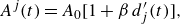 \begin{equation} A^j(t)=A_0[1+\beta\, d_j^{\prime}(t)], \end{equation}
where $A_0$
is the initial amplitude, and
$A_0$
is the initial amplitude, and $d_j^{\prime}=U^{j-1}-U^j$
is the rate of change of the distance between the plates. The updated values of
$d_j^{\prime}=U^{j-1}-U^j$
is the rate of change of the distance between the plates. The updated values of $A^j$
are entered in step (i) of the numerical method (§ 2.3), where
$A^j$
are entered in step (i) of the numerical method (§ 2.3), where $V$
is replaced by
$V$
is replaced by $V_j(t)=A^j(t)\,\unicode{x03C0} \cos (\unicode{x03C0} t)$
, and thereby affect all remaining steps (ii)–(v) at each time step.
$V_j(t)=A^j(t)\,\unicode{x03C0} \cos (\unicode{x03C0} t)$
, and thereby affect all remaining steps (ii)–(v) at each time step.


The stabilisation parameter $\beta$
determines how fast the amplitude changes occur as the distance between plates changes. Small values of
$\beta$
determines how fast the amplitude changes occur as the distance between plates changes. Small values of $\beta$
may not be sufficient to prevent collisions in finite time. Large values of
$\beta$
may not be sufficient to prevent collisions in finite time. Large values of $\beta$
lead to fast adjustment, but can also lead to stiffness of the numerical scheme. For all runs shown below, we used
$\beta$
lead to fast adjustment, but can also lead to stiffness of the numerical scheme. For all runs shown below, we used $0.15\leqslant \beta \leqslant 5$
.
$0.15\leqslant \beta \leqslant 5$
.
Figure 7 shows the distances $d_1$
,
$d_1$
, $d_2$
and
$d_2$
and $d_3$
between each pair of plates for a formation of
$d_3$
between each pair of plates for a formation of $n=4$
wings, computed with the stabilisation mechanism. The figure shows that the stabilisation either eliminates or significantly reduces the oscillations in
$n=4$
wings, computed with the stabilisation mechanism. The figure shows that the stabilisation either eliminates or significantly reduces the oscillations in $d_j$
, which quickly approach a steady state. Apart from the smallest value of
$d_j$
, which quickly approach a steady state. Apart from the smallest value of $d_0$
(black curves), all of the collisions observed in figure 6 are avoided, with steady-state solutions approached even in the most unstable case,
$d_0$
(black curves), all of the collisions observed in figure 6 are avoided, with steady-state solutions approached even in the most unstable case, $n=4$
and
$n=4$
and $A=0.1$
. We note that
$A=0.1$
. We note that $d_1$
is not shown with
$d_1$
is not shown with $n=2$
, nor
$n=2$
, nor $d_2$
with
$d_2$
with $n=3$
, since in the absence of collisions, the results are the same as with
$n=3$
, since in the absence of collisions, the results are the same as with $n=4$
. For the sake of clarity, the curves in figure 7 are colour-coded by the equilibrium state that they reach, as opposed to the equilibrium state reached by the corresponding wing pair (
$n=4$
. For the sake of clarity, the curves in figure 7 are colour-coded by the equilibrium state that they reach, as opposed to the equilibrium state reached by the corresponding wing pair ( $n=2$
) in figure 6. Supplementary movie 4 contains examples of simulations with
$n=2$
) in figure 6. Supplementary movie 4 contains examples of simulations with $n=3$
plates, and shows how the stabilisation algorithm prevents a collision between the two trailing plates.
$n=3$
plates, and shows how the stabilisation algorithm prevents a collision between the two trailing plates.
The stabilisation has a significant impact on the vortex wake behind the plates, as an equilibrium state is reached more quickly. In figure 8, we compare snapshots of the vortex sheet behind two plates without (figure 8 a) and with (figure 8 b) stabilisation. Figure 8(a) is the same as shown earlier in figure 3(b), but at a different scale. The formation of a wake of quadrupoles is seen early on (near the plates) in figure 8(a), but no clear pattern emerges far from the plates. On the other hand, the results obtained with stabilisation (figure 8 b) clearly show the emergence of a stable pattern of quadrupoles behind the plates. A positive (negative) vortex is created behind each plate by the plate’s upward (downward) motion. With stabilisation, these four vortices per oscillation period are positioned in a regular stable configuration, which grows slightly in time and space as the plates move forward. Figure 9 shows the vorticity in the wake, corresponding to the regularised vortex sheet shown in figure 8. Figure 9(b) clearly shows the stable pattern in the wake, growing in time and space. The contrast with figure 9(a), which shows much less organised wake vorticity without any growth, is striking.
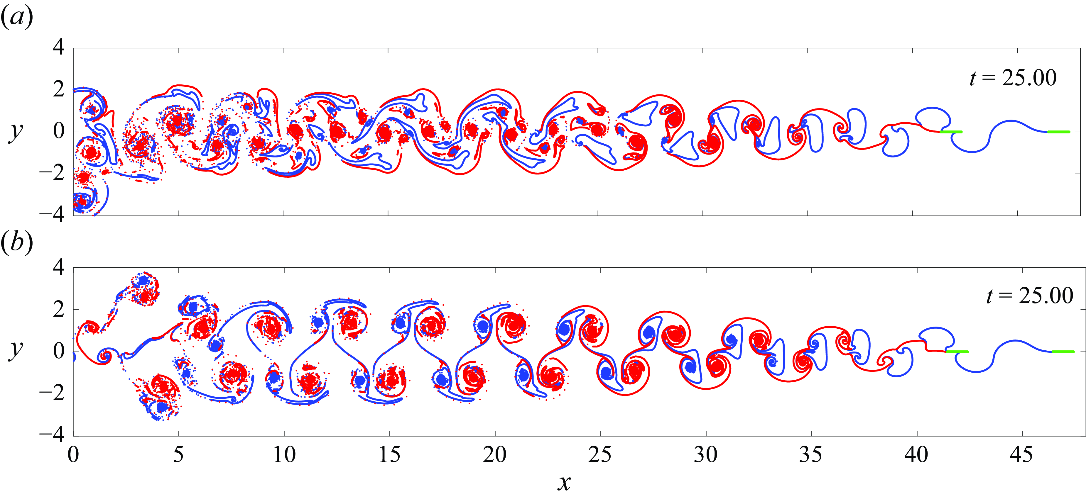
Figure 8. Wake at $t=25$
behind a pair of plates (
$t=25$
behind a pair of plates ( $n=2$
) with heaving amplitude
$n=2$
) with heaving amplitude $A_0=0.2$
and initial separation distance
$A_0=0.2$
and initial separation distance $d_0 = 4.2$
. The plots are (a) without stabilisation, and (b) stabilised according to (3.3) with
$d_0 = 4.2$
. The plots are (a) without stabilisation, and (b) stabilised according to (3.3) with $\beta =2$
.
$\beta =2$
.
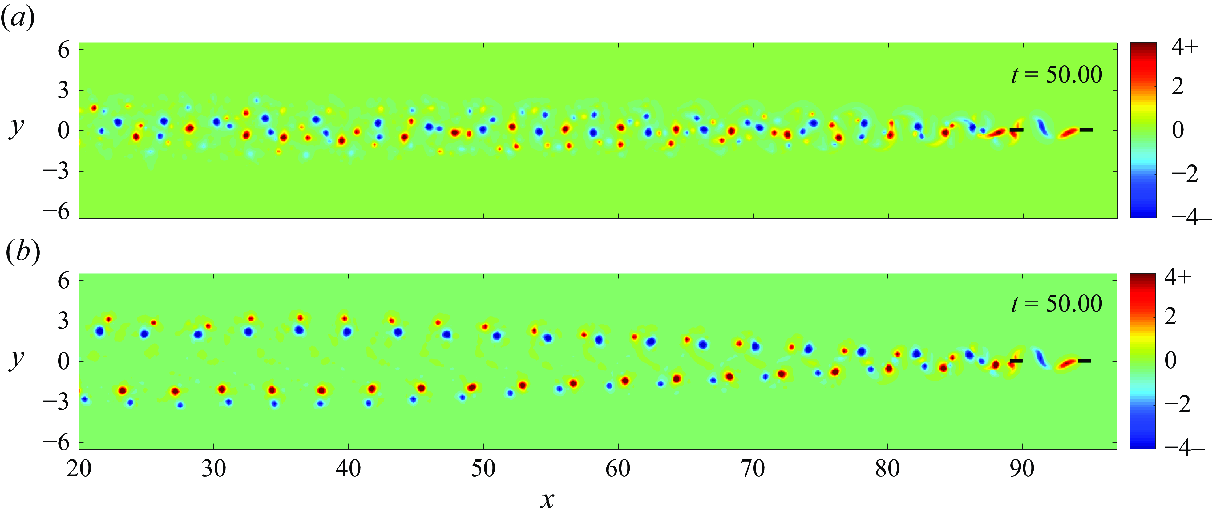
Figure 9. Vorticity at $t=50$
, with the same parameters as in figure 8.
$t=50$
, with the same parameters as in figure 8.
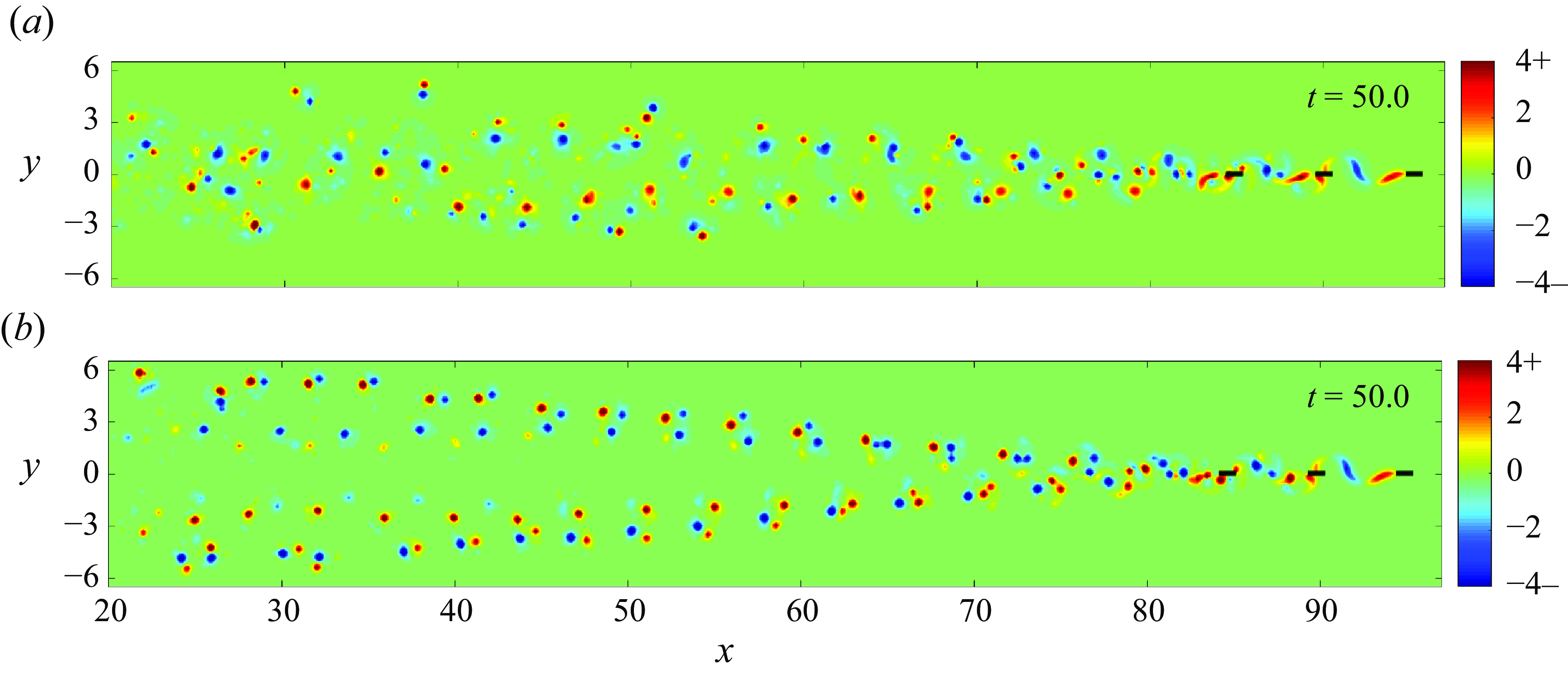
Figure 10. Vorticity at $t=50$
behind three plates (
$t=50$
behind three plates ( $n=3$
) with heaving amplitude
$n=3$
) with heaving amplitude $A_0=0.2$
and initial separation distance
$A_0=0.2$
and initial separation distance $d_0 = 4.2$
. The plots are (a) without stabilisation, and (b) stabilised according to (3.3) with
$d_0 = 4.2$
. The plots are (a) without stabilisation, and (b) stabilised according to (3.3) with $\beta =2$
.
$\beta =2$
.
Figure 10 shows the vorticity in the wake of $n=3$
plates, with and without stabilisation. Here, each heaving cycle of the three plates generates six vortices per period. Without stabilisation (figure 10
a), the vortices exhibit a coherent pattern only at short times after separation, but they become less organised further downstream. By contrast, with stabilisation (figure 10
b), a regular configuration of six vortices per period clearly emerges. The width of the wake grows in time and space, as was the case for a pair of plates (
$n=3$
plates, with and without stabilisation. Here, each heaving cycle of the three plates generates six vortices per period. Without stabilisation (figure 10
a), the vortices exhibit a coherent pattern only at short times after separation, but they become less organised further downstream. By contrast, with stabilisation (figure 10
b), a regular configuration of six vortices per period clearly emerges. The width of the wake grows in time and space, as was the case for a pair of plates ( $n=2$
, figure 9
b).
$n=2$
, figure 9
b).
We were unable to compute such stable patterns of eight vortices per period in the wake of $n=4$
plates due to the computational cost of doing so. While the stabilisation mechanism allows stable schooling modes to be achieved relatively quickly, the vortex configurations take longer to reach equilibrium. Long time simulations using fast tree-algorithms (Greengard & Rokhlin Reference Greengard and Rokhlin1987; Wang, Krasny & Tlupova Reference Wang, Krasny and Tlupova2020) can be performed in the future to study this phenomenon further.
$n=4$
plates due to the computational cost of doing so. While the stabilisation mechanism allows stable schooling modes to be achieved relatively quickly, the vortex configurations take longer to reach equilibrium. Long time simulations using fast tree-algorithms (Greengard & Rokhlin Reference Greengard and Rokhlin1987; Wang, Krasny & Tlupova Reference Wang, Krasny and Tlupova2020) can be performed in the future to study this phenomenon further.
3.6. Reduced model based on thin-aerofoil theory
We now propose and analyse a reduced model to provide rationale for two of the phenomena observed in our simulations (§ 3.4), namely, that collectives of heaving plates in an in-line formation are increasingly stabilised as the flapping amplitude is increased progressively, and such collectives become less stable as the number of plates increases. To that end, we deploy the seminal thin-aerofoil theory of Wu (Reference Wu1961), who considered the motion of a single flat plate executing a small amplitude heaving motion ( $A \ll 1$
) while translating horizontally at velocity
$A \ll 1$
) while translating horizontally at velocity $U$
in an inviscid and incompressible two-dimensional fluid. To simplify the problem, the plate is assumed to shed a flat vortex sheet from its trailing edge, and the sheet strength is determined by the Kutta condition. By solving the linearised Euler equations using conformal mapping, the (dimensionless) thrust
$U$
in an inviscid and incompressible two-dimensional fluid. To simplify the problem, the plate is assumed to shed a flat vortex sheet from its trailing edge, and the sheet strength is determined by the Kutta condition. By solving the linearised Euler equations using conformal mapping, the (dimensionless) thrust $T_0$
on the plate is found to be
$T_0$
on the plate is found to be
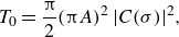 \begin{align} T_0 = \frac {\unicode{x03C0} }{2}(\unicode{x03C0} A)^2\,|C(\sigma)|^2,\end{align}
where
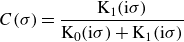 \begin{align} C(\sigma)=\frac {\mathrm{K}_1(\mathrm{i}\sigma)}{\mathrm{K}_0(\mathrm{i}\sigma)+\mathrm{K}_1(\mathrm{i}\sigma)} \end{align}
is the so-called Theodorsen function, $\mathrm{K}_{0,1}$
are the modified Bessel functions of the second kind of orders zero and one, and
$\mathrm{K}_{0,1}$
are the modified Bessel functions of the second kind of orders zero and one, and $\sigma = \unicode{x03C0} /(2U)$
is the reduced frequency. An analogous theory has been developed to describe how a follower plate located downstream of the leader and executing the same heaving kinematics would be affected by the leader’s wake (Wu & Chwang Reference Wu and Chwang1975; Ramananarivo et al. Reference Ramananarivo, Fang, Oza, Zhang and Ristroph2016). In this theory, the no-penetration boundary condition is not satisfied simultaneously on both wings; instead, an approximation for the hydrodynamic thrust on the follower is found by assuming that the leader’s wake is unaffected by the follower’s presence. This assumption is consistent with our numerical simulations before the leader’s wake has reached the follower, as discussed in § 3.2. This thrust is found to be
$\sigma = \unicode{x03C0} /(2U)$
is the reduced frequency. An analogous theory has been developed to describe how a follower plate located downstream of the leader and executing the same heaving kinematics would be affected by the leader’s wake (Wu & Chwang Reference Wu and Chwang1975; Ramananarivo et al. Reference Ramananarivo, Fang, Oza, Zhang and Ristroph2016). In this theory, the no-penetration boundary condition is not satisfied simultaneously on both wings; instead, an approximation for the hydrodynamic thrust on the follower is found by assuming that the leader’s wake is unaffected by the follower’s presence. This assumption is consistent with our numerical simulations before the leader’s wake has reached the follower, as discussed in § 3.2. This thrust is found to be $T = T_0 [1+F(d)]$
, where
$T = T_0 [1+F(d)]$
, where $d$
is the distance between the leader’s trailing edge and the follower’s leading edge (as in figure 1), and
$d$
is the distance between the leader’s trailing edge and the follower’s leading edge (as in figure 1), and
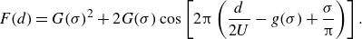 \begin{align} F(d) &= G(\sigma)^2+2G(\sigma)\cos \left [2\unicode{x03C0} \left (\frac {d}{2U}-g(\sigma)+\frac {\sigma }{\unicode{x03C0} }\right)\right]. \end{align}
Here, the real-valued functions $G(\sigma)$
and
$G(\sigma)$
and $g(\sigma)$
are defined through the relation
$g(\sigma)$
are defined through the relation
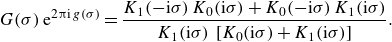 \begin{align} G(\sigma)\,\mathrm{e}^{2\unicode{x03C0} \mathrm{i}\, g(\sigma)}&= \frac {{K}_1(-\mathrm{i}\sigma)\,{K}_0(\mathrm{i}\sigma)+{K}_0(-\mathrm{i}\sigma)\,{K}_1(\mathrm{i}\sigma)}{{K}_1(\mathrm{i}\sigma)\,\left [{K}_0(\mathrm{i}\sigma)+{K}_1(\mathrm{i}\sigma)\right]}. \end{align}
We thus propose the following model for a collective of $n$
plates that execute small-amplitude heaving kinematics in an in-line formation:
$n$
plates that execute small-amplitude heaving kinematics in an in-line formation:
 \begin{align} M\ddot {x}_1+C_{{d}}\dot {x}_1^{3/2}&=T_0,\nonumber \\ M\ddot {x}_m+C_{{d}}\dot {x}_m^{3/2}&=T_0\left [1+F(x_{m-1}-x_{m}-1)\right], \quad 2\leqslant m\leqslant n, \end{align}
where $x_m$
is the horizontal position of the centre of the
$x_m$
is the horizontal position of the centre of the $m$
th plate. We have assumed that each plate is influenced only by its nearest upstream neighbour; that is, the leader wing (
$m$
th plate. We have assumed that each plate is influenced only by its nearest upstream neighbour; that is, the leader wing ( $x_1$
) is unaffected by all of the followers, and moves at a steady speed
$x_1$
) is unaffected by all of the followers, and moves at a steady speed $U$
determined by the balance between drag and thrust forces on it:
$U$
determined by the balance between drag and thrust forces on it:
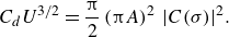 \begin{align} C_{{d}}U^{3/2}&=\frac {\unicode{x03C0} }{2}\left (\unicode{x03C0} A\right)^2\,|C(\sigma)|^2. \end{align}
Every other wing is influenced by its upstream neighbour through the function $F$
, which depends on the steady speed
$F$
, which depends on the steady speed $U$
. That is, our theory is valid in the quasi-steady regime in which the wings’ velocities are all close to
$U$
. That is, our theory is valid in the quasi-steady regime in which the wings’ velocities are all close to $U$
. The nearest-neighbour assumption may be justified using our simulations that employ stabilisation (figure 7); specifically,
$U$
. The nearest-neighbour assumption may be justified using our simulations that employ stabilisation (figure 7); specifically, $d_1^{\infty,k}\approx d_2^{\infty,k}\approx d_3^{\infty,k}$
, which suggests that the equilibrium distances are mostly insensitive to the number of upstream wings. The assumption is also supported by recent experiments on up to five flapping hydrofoils in an in-line formation (Newbolt et al. Reference Newbolt, Lewis, Bleu, Wu, Mavroyiakoumou, Ramananarivo and Ristroph2024). Table 1 shows a comparison between the steady speeds
$d_1^{\infty,k}\approx d_2^{\infty,k}\approx d_3^{\infty,k}$
, which suggests that the equilibrium distances are mostly insensitive to the number of upstream wings. The assumption is also supported by recent experiments on up to five flapping hydrofoils in an in-line formation (Newbolt et al. Reference Newbolt, Lewis, Bleu, Wu, Mavroyiakoumou, Ramananarivo and Ristroph2024). Table 1 shows a comparison between the steady speeds $U$
obtained in our vortex sheet simulations and those predicted from (3.9), with surprisingly good agreement given the simplified nature of our reduced model.
$U$
obtained in our vortex sheet simulations and those predicted from (3.9), with surprisingly good agreement given the simplified nature of our reduced model.
Table 1. The values of the velocity $U$
of a single wing, as obtained in our vortex sheet simulations (§ 3.1) and predicted by thin-aerofoil theory from (3.9), are shown for different values of the flapping amplitude
$U$
of a single wing, as obtained in our vortex sheet simulations (§ 3.1) and predicted by thin-aerofoil theory from (3.9), are shown for different values of the flapping amplitude $A$
.
$A$
.
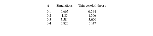
We proceed by seeking steadily translating solutions of (3.8), in which the wings move at a constant speed $U$
with a constant separation distance
$U$
with a constant separation distance $d$
between them,
$d$
between them, $x_{m}(t)-x_{m+1}(t)=d+1$
. By substituting the form
$x_{m}(t)-x_{m+1}(t)=d+1$
. By substituting the form $x_m(t)=Ut-(m-1)(d+1)$
into (3.8), we find that
$x_m(t)=Ut-(m-1)(d+1)$
into (3.8), we find that $d$
satisfies the algebraic equation
$d$
satisfies the algebraic equation
 \begin{align} F(d)=0. \end{align}
This equation has infinitely many positive solutions $d^{\infty,k}$
for
$d^{\infty,k}$
for $k\in \mathbb{Z}_{\gt 0}$
. For the parameter values adopted in this paper,
$k\in \mathbb{Z}_{\gt 0}$
. For the parameter values adopted in this paper, $M = 1$
,
$M = 1$
, $C_{{d}}=0.1$
and
$C_{{d}}=0.1$
and $A = 0.1{-}0.4$
, we find that the corresponding schooling numbers
$A = 0.1{-}0.4$
, we find that the corresponding schooling numbers $S_k=d^{\infty,k}/(2U)$
are equal to
$S_k=d^{\infty,k}/(2U)$
are equal to $S_1+k-1$
, where
$S_1+k-1$
, where $S_1$
is between 0.95 and 1.1, in good agreement with values obtained in our vortex sheet simulations (figure 6). We note that a similar result was obtained for two plates by Ramananarivo et al. (Reference Ramananarivo, Fang, Oza, Zhang and Ristroph2016) using a similar thin-aerofoil theory, and by Baddoo et al. (Reference Baddoo, Moore, Oza and Crowdy2023) using a more sophisticated thin-aerofoil theory based on conformal maps of multiply connected domains. Reduced models of flapping wings that approximate the hydrodynamic interactions using time-delay differential equations also recover near-integer values of the equilibrium schooling numbers (Heydari, Hang & Kanso Reference Heydari, Hang and Kanso2024; Newbolt et al. Reference Newbolt, Lewis, Bleu, Wu, Mavroyiakoumou, Ramananarivo and Ristroph2024). We also note that (3.10) is satisfied by a second family of solutions with schooling numbers
$S_1$
is between 0.95 and 1.1, in good agreement with values obtained in our vortex sheet simulations (figure 6). We note that a similar result was obtained for two plates by Ramananarivo et al. (Reference Ramananarivo, Fang, Oza, Zhang and Ristroph2016) using a similar thin-aerofoil theory, and by Baddoo et al. (Reference Baddoo, Moore, Oza and Crowdy2023) using a more sophisticated thin-aerofoil theory based on conformal maps of multiply connected domains. Reduced models of flapping wings that approximate the hydrodynamic interactions using time-delay differential equations also recover near-integer values of the equilibrium schooling numbers (Heydari, Hang & Kanso Reference Heydari, Hang and Kanso2024; Newbolt et al. Reference Newbolt, Lewis, Bleu, Wu, Mavroyiakoumou, Ramananarivo and Ristroph2024). We also note that (3.10) is satisfied by a second family of solutions with schooling numbers $\tilde {S}_k=\tilde {S}_1+k-1$
, where
$\tilde {S}_k=\tilde {S}_1+k-1$
, where $\tilde {S}_1$
is between 0.6 and 0.7 for the parameter values adopted in this paper. We neglect these solutions in the forthcoming discussion because they are linearly unstable to perturbations and thus not observed in our simulations or in laboratory experiments (Ramananarivo et al. Reference Ramananarivo, Fang, Oza, Zhang and Ristroph2016).
$\tilde {S}_1$
is between 0.6 and 0.7 for the parameter values adopted in this paper. We neglect these solutions in the forthcoming discussion because they are linearly unstable to perturbations and thus not observed in our simulations or in laboratory experiments (Ramananarivo et al. Reference Ramananarivo, Fang, Oza, Zhang and Ristroph2016).
We now examine the linear stability of the state in which the distance between each pair of wings corresponds to the schooling number $S_1$
, the analysis of the other schooling numbers
$S_1$
, the analysis of the other schooling numbers $S_k$
being identical due to the periodicity of the function
$S_k$
being identical due to the periodicity of the function $F$
. To that end, we substitute the form
$F$
. To that end, we substitute the form $x_m(t)=Ut-(m-1) (d^{\infty,1}+1)+\epsilon\, \tilde {x}_m(t)$
into (3.8), and retain terms at leading order in
$x_m(t)=Ut-(m-1) (d^{\infty,1}+1)+\epsilon\, \tilde {x}_m(t)$
into (3.8), and retain terms at leading order in $\epsilon$
. The linearised equations are thus (dropping the tildes)
$\epsilon$
. The linearised equations are thus (dropping the tildes)
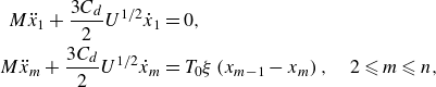 \begin{align} M\ddot {x}_1+\frac {3C_{{d}}}{2}U^{1/2}\dot {x}_1&=0,\nonumber \\ M\ddot {x}_m+\frac {3C_{{d}}}{2}U^{1/2}\dot {x}_m&=T_0\xi \left (x_{m-1}-x_{m}\right),\quad 2\leqslant m\leqslant n, \end{align}
where $\xi = F^{\prime } (d^{\infty,1})$
. We assume that an impulsive perturbation is applied to the leader:
$\xi = F^{\prime } (d^{\infty,1})$
. We assume that an impulsive perturbation is applied to the leader:
 \begin{align} x_1(0)=1,\quad \dot {x}_1(0)=s_1\equiv -\frac {3C_{{d}}U^{1/2}}{2M}\quad \mathrm{and} \quad x_m(0)=\dot {x}_m(0)=0\ \text{for}\ m\geqslant 2. \end{align}
It is straightforward to obtain the solutions
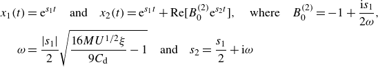 \begin{align} x_1(t)&={\rm e}^{s_1t}\quad\mathrm{and}\quad x_2(t)={\rm e}^{s_1t} + \mathrm{Re}\big[B_0^{(2)}{\rm e}^{s_2t}\big],\quad \mathrm{where}\quad B_0^{(2)}=-1+\frac{{\rm i} s_1}{2\omega},\nonumber \\\omega &= \frac{|s_1|}{2}\sqrt{\frac{16MU^{1/2}\xi}{9C_{\mathrm{d}}}-1}\quad\mathrm{and}\quad s_2=\frac{s_1}{2}+{\rm i}\omega \end{align}
is a root of the quadratic polynomial $p(s)\equiv Ms^2+(3C_{{d}}/2)U^{1/2}s+T_0\xi$
. We find that
$p(s)\equiv Ms^2+(3C_{{d}}/2)U^{1/2}s+T_0\xi$
. We find that $\omega \in \mathbb{R}$
for the parameter values adopted in this paper. Each wing after the second oscillates in resonance with its upstream neighbour, so the general solution to (3.11) has the form
$\omega \in \mathbb{R}$
for the parameter values adopted in this paper. Each wing after the second oscillates in resonance with its upstream neighbour, so the general solution to (3.11) has the form
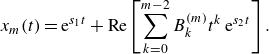 \begin{align} x_m(t)=\mathrm{e}^{s_1t}+\mathrm{Re}\left [\sum _{k=0}^{m-2}B_k^{(m)}t^k\,\mathrm{e}^{s_2t}\right]. \end{align}
The coefficients $B_0^{(m)}$
may be obtained using the initial conditions:
$B_0^{(m)}$
may be obtained using the initial conditions:
 \begin{align} B_0^{(m)}=-1+\frac {\mathrm{i}}{\omega }\left (\frac {s_1}{2}+\mathrm{Re}\left [B_1^{(m)}\right]\right),\quad m\geqslant 3. \end{align}
To obtain the remaining coefficients, we write (3.11) in the compact form $\mathcal{L}x_m=T_0\xi x_{m-1}$
for
$\mathcal{L}x_m=T_0\xi x_{m-1}$
for $m\geqslant 2$
, where
$m\geqslant 2$
, where $\mathcal{L}=p(\mathrm{d}/\mathrm{d} t)$
. Using the facts that
$\mathcal{L}=p(\mathrm{d}/\mathrm{d} t)$
. Using the facts that
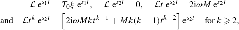 \begin{align} \mathcal{L}\,\mathrm{e}^{s_1t}&=T_0\xi\, \mathrm{e}^{s_1t},\quad \mathcal{L}\,\mathrm{e}^{s_2t}=0,\quad \mathcal{L}t\,\mathrm{e}^{s_2t}=2\mathrm{i}\omega M\,\mathrm{e}^{s_2t}\nonumber \\ \mathrm{and}\quad \mathcal{L}t^k\,\mathrm{e}^{s_2t}&=\left [2\mathrm{i}\omega Mkt^{k-1}+Mk(k-1)t^{k-2}\right]\mathrm{e}^{s_2t}\quad \mathrm{for}\ k\geqslant 2, \end{align}
it can be shown that the coefficients $B_k^{(m)}$
satisfy the recursion relation
$B_k^{(m)}$
satisfy the recursion relation
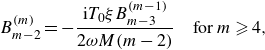 \begin{align} &B_{m-2}^{(m)}=-\frac {\mathrm{i} T_0\xi B_{m-3}^{(m-1)}}{2\omega M(m-2)}\quad \mathrm{for}\ m\geqslant 4, \end{align}
 \begin{align} &2\mathrm{i}\omega MB_{k+1}^{(m)}(k+1)+MB_{k+2}^{(m)} (k+1)(k+2)=T_0\xi B_k^{(m-1)}\quad \mathrm{for}\ k=0,\ldots,m-4. \end{align}
Taken together, (3.15) and (3.17) determine all of the coefficients in the solution (3.14).
We proceed by making two observations about this solution. First, the equilibrium schooling states are linearly stable because the perturbations decay in time, $x_m(t)\rightarrow 0$
as
$x_m(t)\rightarrow 0$
as $t\rightarrow \infty$
. Moreover, the decay rate
$t\rightarrow \infty$
. Moreover, the decay rate $s_1/2$
increases with
$s_1/2$
increases with $U$
, as is evident from (3.12), and thus with the flapping amplitude
$U$
, as is evident from (3.12), and thus with the flapping amplitude $A$
, providing a rationale for the observation from our vortex sheet simulations (§ 3.4) that a larger flapping amplitude stabilises the schooling state. Second, by plotting the solution (3.14) for the parameter values adopted in this paper, we observe that the perturbations are amplified downstream, in that at intermediate times they exhibit oscillations that grow in time and have progressively larger amplitude as
$A$
, providing a rationale for the observation from our vortex sheet simulations (§ 3.4) that a larger flapping amplitude stabilises the schooling state. Second, by plotting the solution (3.14) for the parameter values adopted in this paper, we observe that the perturbations are amplified downstream, in that at intermediate times they exhibit oscillations that grow in time and have progressively larger amplitude as $m$
increases. To see why this is the case, we observe that the exponential decay factors
$m$
increases. To see why this is the case, we observe that the exponential decay factors $\mathrm{e}^{s_2t}$
in (3.14) are multiplied by increasingly large powers of
$\mathrm{e}^{s_2t}$
in (3.14) are multiplied by increasingly large powers of $t$
as
$t$
as $m$
increases. More precisely, note that (3.17a
) can be solved explicitly for
$m$
increases. More precisely, note that (3.17a
) can be solved explicitly for $B_{m-2}^{(m)}$
, from which the long-time asymptotic behaviour of
$B_{m-2}^{(m)}$
, from which the long-time asymptotic behaviour of $x_m(t)$
can be deduced:
$x_m(t)$
can be deduced:
 \begin{align} x_m(t)\sim \text{Re}[X_m(t)]\ \text{as}\ t\rightarrow \infty,\quad \text{where}\ X_m(t)=\frac {B_0^{(2)}}{(m-2)!}\left (\frac {-\mathrm{i} T_0\xi }{2\omega M}\right)^{m-2}t^{m-2}\,\mathrm{e}^{s_2t}. \end{align}
We find that for the parameter values adopted in this paper, $|X_m(t)|$
provides an adequate approximation for the envelope of the oscillating solution
$|X_m(t)|$
provides an adequate approximation for the envelope of the oscillating solution $x_m(t)$
in (3.14). Moreover, it is easy to see that
$x_m(t)$
in (3.14). Moreover, it is easy to see that $|X_m(t)|\propto t^{m-2}\,\mathrm{e}^{s_1t/2}$
attains its maximum value
$|X_m(t)|\propto t^{m-2}\,\mathrm{e}^{s_1t/2}$
attains its maximum value
 \begin{align} X_m^*\equiv |X_m(t_m)|=\frac {\left |B_0^{(2)}\right |}{(m-2)!}\left (\frac {T_0\xi (m-2)}{\omega M|s_1|\mathrm{e}}\right)^{m-2}\quad \text{at the time}\ t=t_m\equiv \frac {2(m-2)}{|s_1|}. \end{align}
By using Stirling’s formula, $m!\sim \sqrt {2\unicode{x03C0} m}\,(m/\mathrm{e})^m$
as
$m!\sim \sqrt {2\unicode{x03C0} m}\,(m/\mathrm{e})^m$
as $m\rightarrow \infty$
, we conclude that the peak of the envelope
$m\rightarrow \infty$
, we conclude that the peak of the envelope $X_m^*$
increases with
$X_m^*$
increases with $m$
for sufficiently large
$m$
for sufficiently large $m$
provided that
$m$
provided that $T_0\xi /(\omega M\,|s_1|) \gt 1$
, as is the case for the parameter values adopted in this paper. Moreover, the time
$T_0\xi /(\omega M\,|s_1|) \gt 1$
, as is the case for the parameter values adopted in this paper. Moreover, the time $t_m$
at which the peak is attained increases with
$t_m$
at which the peak is attained increases with $m$
, which further illustrates that the oscillations propagate downstream. The linear theory thus provides a qualitative rationale for the observation from our vortex sheet simulations (§ 3.4) that the schooling states become less stable as the number of wings increases.
$m$
, which further illustrates that the oscillations propagate downstream. The linear theory thus provides a qualitative rationale for the observation from our vortex sheet simulations (§ 3.4) that the schooling states become less stable as the number of wings increases.
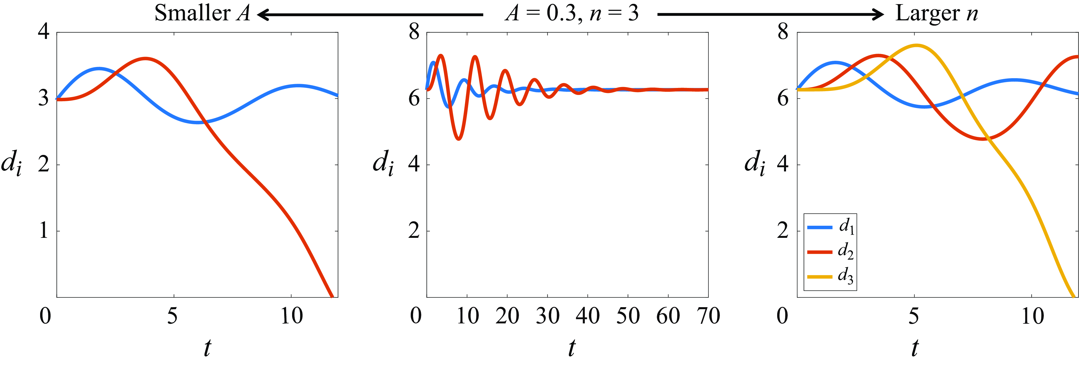
Figure 11. Results of numerical simulations of the (nonlinear) reduced model (3.8). The initial velocity of the leader is $1.3U$
, and the remaining plates are initialised in an equilibrium schooling mode with velocity
$1.3U$
, and the remaining plates are initialised in an equilibrium schooling mode with velocity $U$
(given by (3.9)) and inter-plate distance
$U$
(given by (3.9)) and inter-plate distance $d^{\infty,1}$
(given by (3.10)). The middle panel shows the inter-plate distances for
$d^{\infty,1}$
(given by (3.10)). The middle panel shows the inter-plate distances for $n=3$
wings flapping with amplitude
$n=3$
wings flapping with amplitude $A=0.3$
; after a transient, the system returns to the equilibrium schooling state. The right-hand panel shows the effect of adding a plate (
$A=0.3$
; after a transient, the system returns to the equilibrium schooling state. The right-hand panel shows the effect of adding a plate ( $A = 0.3$
,
$A = 0.3$
, $n=4$
), and the left-hand panel shows the effect of decreasing the flapping amplitude (
$n=4$
), and the left-hand panel shows the effect of decreasing the flapping amplitude ( $A=0.2$
,
$A=0.2$
, $n=3$
). It is evident that both lead to a collision between the trailing plates.
$n=3$
). It is evident that both lead to a collision between the trailing plates.
While the foregoing linear theory predicts that small-amplitude perturbations to the equilibrium schooling state eventually decay in time, we find that transient linear growth combined with nonlinear effects can cause finite-amplitude perturbations to dislodge the trailing plates from their equilibrium positions. Specifically, we performed numerical simulations of the nonlinear reduced model (3.8), initialising the plates with the positions $x_m(0)=-(m-1) (d^{\infty,1}+1)$
and velocities
$x_m(0)=-(m-1) (d^{\infty,1}+1)$
and velocities $\dot {x}_m(0)=U$
for
$\dot {x}_m(0)=U$
for $m \gt 1$
and
$m \gt 1$
and $\dot {x}_1(0)=1.3U$
; that is, we assume that the trailing wings initially move with the steady speed of a single wing, as determined by (3.9), and subject the leader to a finite-amplitude velocity perturbation. The results are shown in figure 11. The middle panel shows the inter-plate distances
$\dot {x}_1(0)=1.3U$
; that is, we assume that the trailing wings initially move with the steady speed of a single wing, as determined by (3.9), and subject the leader to a finite-amplitude velocity perturbation. The results are shown in figure 11. The middle panel shows the inter-plate distances $d_i$
for
$d_i$
for $n = 3$
wings and flapping amplitude
$n = 3$
wings and flapping amplitude $A = 0.3$
: after a transient, the trailing wings eventually settle back into their equilibrium positions. By contrast, increasing the number of wings to
$A = 0.3$
: after a transient, the trailing wings eventually settle back into their equilibrium positions. By contrast, increasing the number of wings to $n = 4$
(right-hand panel) or decreasing the flapping amplitude to
$n = 4$
(right-hand panel) or decreasing the flapping amplitude to $A = 0.2$
(left-hand panel) causes the trailing wings to become dislodged from their equilibrium positions and collide. A qualitatively similar behaviour is observed for the other flapping amplitudes considered in this paper. We thus conclude that despite its simplifications, the reduced model presented in this section captures the two salient features of our vortex sheet simulations, namely, that schooling modes become progressively less stable as the number of wings is increased or the flapping amplitude is decreased.
$A = 0.2$
(left-hand panel) causes the trailing wings to become dislodged from their equilibrium positions and collide. A qualitatively similar behaviour is observed for the other flapping amplitudes considered in this paper. We thus conclude that despite its simplifications, the reduced model presented in this section captures the two salient features of our vortex sheet simulations, namely, that schooling modes become progressively less stable as the number of wings is increased or the flapping amplitude is decreased.
We note that a number of physical effects are neglected in our reduced model (3.8) for the sake of analytical simplicity. Specifically, the assumptions are that the wake shed by each plate is flat and unaffected by modulations in the plate’s horizontal speed, both of which are at odds with our vortex sheet simulations. The model also assumes nearest-upstream-neighbour interactions; while our simulation results seem to confirm this assumption (§ 3.2), strictly speaking each plate feels the vortex sheets shed by all of the other plates.
4. Conclusion
In this paper, we have used a vortex sheet method to simulate the dynamics of $n$
flat plates in a two-dimensional inviscid and incompressible fluid. The plates are in an in-line formation and execute a heaving kinematics with amplitude
$n$
flat plates in a two-dimensional inviscid and incompressible fluid. The plates are in an in-line formation and execute a heaving kinematics with amplitude $A$
and frequency
$A$
and frequency $f$
(figure 1), but their horizontal velocities are determined by the balance of hydrodynamic thrust and drag forces. The thrust forces are induced by the vortex sheet strength at the leading edge, which in turn is induced by the prescribed vertical motion and the fluid vorticity. The drag forces depend on the plate velocity and are modelled using a simple
$f$
(figure 1), but their horizontal velocities are determined by the balance of hydrodynamic thrust and drag forces. The thrust forces are induced by the vortex sheet strength at the leading edge, which in turn is induced by the prescribed vertical motion and the fluid vorticity. The drag forces depend on the plate velocity and are modelled using a simple $3/2$
power law. Particular care is taken to evaluate the near-singular integrals that arise when a vortex sheet is near a plate, which is required both to ensure that the vortex sheet does not cross the plate and to accurately compute the hydrodynamic thrust on the plate.
$3/2$
power law. Particular care is taken to evaluate the near-singular integrals that arise when a vortex sheet is near a plate, which is required both to ensure that the vortex sheet does not cross the plate and to accurately compute the hydrodynamic thrust on the plate.
We find that the long-time motion of a single plate is independent of the imposed initial velocity $U_0$
(figure 2). The plate moves forward in an oscillatory manner due to the oscillatory leading edge sheet strength, and leaves a wake of positive and negative vortices, one of each being formed during one oscillation period (figure 4
a). The wake of
$U_0$
(figure 2). The plate moves forward in an oscillatory manner due to the oscillatory leading edge sheet strength, and leaves a wake of positive and negative vortices, one of each being formed during one oscillation period (figure 4
a). The wake of $n$
plates consists of
$n$
plates consists of $2n$
vortices generated in each oscillation period, which interact and form a quasi-periodic pattern with wavelength
$2n$
vortices generated in each oscillation period, which interact and form a quasi-periodic pattern with wavelength $U_{\infty }/f$
(figures 4
b–d).
$U_{\infty }/f$
(figures 4
b–d).
Our simulations show that plates in the wake of prior ones move towards certain equilibrium positions (figure 5). These equilibria are quantised on the schooling number (Becker et al. Reference Becker, Masoud, Newbolt, Shelley and Ristroph2015): that is, the distance between a given plate and the one in front of it is approximately an integer multiple of the wavelength $U_{\infty }/f$
. This observation is consistent with prior experiments and vortex sheet simulations of both pairs (Fang Reference Fang2016; Ramananarivo et al. Reference Ramananarivo, Fang, Oza, Zhang and Ristroph2016; Heydari & Kanso Reference Heydari and Kanso2021) and larger collectives (Newbolt et al. Reference Newbolt, Zhang and Ristroph2022, Reference Newbolt, Lewis, Bleu, Wu, Mavroyiakoumou, Ramananarivo and Ristroph2024; Heydari, Hang & Kanso Reference Heydari, Hang and Kanso2024) of flapping wings. By varying the initial distance
$U_{\infty }/f$
. This observation is consistent with prior experiments and vortex sheet simulations of both pairs (Fang Reference Fang2016; Ramananarivo et al. Reference Ramananarivo, Fang, Oza, Zhang and Ristroph2016; Heydari & Kanso Reference Heydari and Kanso2021) and larger collectives (Newbolt et al. Reference Newbolt, Zhang and Ristroph2022, Reference Newbolt, Lewis, Bleu, Wu, Mavroyiakoumou, Ramananarivo and Ristroph2024; Heydari, Hang & Kanso Reference Heydari, Hang and Kanso2024) of flapping wings. By varying the initial distance $d_0$
between each plate and its upstream neighbour, we find the first six equilibrium positions for
$d_0$
between each plate and its upstream neighbour, we find the first six equilibrium positions for $n=2$
, 3 and 4 plates, for the three dimensionless flapping amplitudes
$n=2$
, 3 and 4 plates, for the three dimensionless flapping amplitudes $A=0.1$
, 0.3 and 0.4 (figure 6). Which equilibrium is approached by a trailing plate depends on its initial distance from the preceding one.
$A=0.1$
, 0.3 and 0.4 (figure 6). Which equilibrium is approached by a trailing plate depends on its initial distance from the preceding one.
As more plates are added to the formation, they experience increasingly large oscillations in their horizontal motion. This is apparent, for instance, by comparing the three panels in the top row of figure 6, for which the flapping amplitude is $A = 0.4$
. The basins of attraction of the equilibrium positions evidently shrink, as evidenced by the trajectories that depart from the equilibria altogether. For smaller values of the flapping amplitude, the in-line formation becomes increasingly unstable, with a number of cases in which the plates not only leave their nearest equilibria but collide with their upstream neighbours. The loss of stability and associated collisions are far more prevalent both as the number of plates
$A = 0.4$
. The basins of attraction of the equilibrium positions evidently shrink, as evidenced by the trajectories that depart from the equilibria altogether. For smaller values of the flapping amplitude, the in-line formation becomes increasingly unstable, with a number of cases in which the plates not only leave their nearest equilibria but collide with their upstream neighbours. The loss of stability and associated collisions are far more prevalent both as the number of plates $n$
increases and as the amplitude
$n$
increases and as the amplitude $A$
decreases. For example, for
$A$
decreases. For example, for $A=0.1$
,
$A=0.1$
, $n=4$
, less than a third of the initial conditions tested have not collided after thirty flapping periods.
$n=4$
, less than a third of the initial conditions tested have not collided after thirty flapping periods.
We find that a simple algorithm is sufficient to mitigate the flow-induced instability that we observe: specifically, if a plate approaches (separates from) its upstream neighbour, then it slows down (speeds up) by adjusting its flapping amplitude $A$
. This leads to out-of-sync oscillations until an equilibrium position is reached (figure 7). The stabilised vortex wakes form beautiful organised vortex patterns that are not observed without stabilisation (figures 9 and 10). The stabilised wakes are expected to represent the long-time limit of unstabilised wakes that have not lost stability and reached an equilibrium. The cost of such long-time computations is prohibitive, and the stabilisation scheme enables us compute these patterns in reasonable time, at least for
$A$
. This leads to out-of-sync oscillations until an equilibrium position is reached (figure 7). The stabilised vortex wakes form beautiful organised vortex patterns that are not observed without stabilisation (figures 9 and 10). The stabilised wakes are expected to represent the long-time limit of unstabilised wakes that have not lost stability and reached an equilibrium. The cost of such long-time computations is prohibitive, and the stabilisation scheme enables us compute these patterns in reasonable time, at least for $n=2$
and 3.
$n=2$
and 3.
We have also developed a reduced model for the dynamics of hydrodynamically interacting plates based on linear thin-aerofoil theory (Wu Reference Wu1961; Wu & Chwang Reference Wu and Chwang1975; Ramananarivo et al. Reference Ramananarivo, Fang, Oza, Zhang and Ristroph2016). In this model, we assume that each plate interacts only with its nearest upstream neighbour, and that each plate sheds a flat vortex sheet that is unperturbed by the other plates. The model is able to recover a number of phenomena observed in our simulations, namely, the quantisation of stable equilibria on the schooling number, the dependence of the translation velocity on the flapping amplitude, and the decreasing stability of the formation as $A$
decreases and
$A$
decreases and $n$
increases.
$n$
increases.
The flow-induced oscillatory instability and subsequent collisions within increasingly large in-line formations are reminiscent of the ‘flonons’ observed in recent experiments on flapping wings in a water tank by Newbolt et al. (Reference Newbolt, Lewis, Bleu, Wu, Mavroyiakoumou, Ramananarivo and Ristroph2024). These authors posited that the formation destabilised via a resonance cascade, a physical picture that is consistent with our reduced model in § 3.6. Such an instability was not observed in the vortex sheet simulations of in-line formations of pitching plates conducted by Heydari, Hang & Kanso (Reference Heydari, Hang and Kanso2024), who instead observed that formations typically destabilised via a loss of cohesion in which trailing plates could not keep up with the rest of the school, and fell behind. We note that one difference between our vortex sheet algorithm and that of Heydari, Hang & Kanso (Reference Heydari, Hang and Kanso2024) is that in the latter, the point vortices shed by the plates are manually removed from the fluid after a prescribed dissipation time (Heydari & Kanso Reference Heydari and Kanso2021). Another difference, which is potentially significant, is that Heydari, Hang & Kanso (Reference Heydari, Hang and Kanso2024) consider plates that undergo pitching oscillations about their leading edges, while our plates undergo heaving oscillations. As a consequence, the horizontal force on the plate is generated entirely by the leading-edge suction in our work, while in their work it is dominated by the pressure force normal to the plate (Heydari & Kanso Reference Heydari and Kanso2021). We also note that we do not observe a ‘compact’ formation in which the plates are separated by less than a chord length, which has been observed in two-dimensional Navier–Stokes simulations of elastic filaments (Zhu et al. Reference Zhu, He and Zhang2014) and wings (Lin et al. Reference Lin, Wu, Zhang and Yang2020) in flows with ${Re} = O(100)$
, and also in three-dimensional Navier–Stokes simulations of flexible plates (Arranz et al. Reference Arranz, Flores and García-Villalba2022).
${Re} = O(100)$
, and also in three-dimensional Navier–Stokes simulations of flexible plates (Arranz et al. Reference Arranz, Flores and García-Villalba2022).
The in-line formation considered herein may be viewed as a minimal model for a fish school, in which only hydrodynamic interactions are considered at the expense of behavioural rules and sensing. Our results suggest that fish may need to employ active control mechanisms to mitigate the flow-induced instability experienced by increasingly large formations, but that relatively simple control mechanisms (like the one proposed in § 3.5) could be sufficient. A worthwhile future direction would be to consider more sophisticated control mechanisms, such as those based on reinforcement learning (Novati et al. Reference Novati, Verma, Alexeev, Rossinelli, van Rees and Koumoutsakos2017; Verma, Novati & Koumoutsakos Reference Verma, Novati and Koumoutsakos2018). One could also explore biologically relevant control mechanisms, such as those inspired by the fish lateral line system, which detects the nearby flow velocity and pressure gradients, and is thought to play an important role in mediating schooling behaviour (Faucher et al. Reference Faucher, Parmentier, Becco, Vandewalle and Vandewalle2010; Mekdara et al. Reference Mekdara, Nasimi, Schwalbe and Tytell2021). While our study was focused on the formation’s streamwise stability, another future direction would be to allow the plates to translate in both the streamwise and lateral directions, and thus examine the two-dimensional stability of various formations, as has been done using models (Gazzola et al. Reference Gazzola, Tchieu, Alexeev, de Brauer and Koumoutsakos2016), Navier–Stokes simulations (Gazzola et al. Reference Gazzola, Chatelain, van Rees and Koumoutsakos2011; Lin et al. Reference Lin, Wu, Zhang and Yang2021, Reference Lin, Wu, Yang and Dong2022) and experiments (Ormonde et al. Reference Ormonde, Kurt, Mivehchi and Moored2023). Moreover, the simulation framework presented herein could be extended straightforwardly to model more complex formations, such as the diamond lattice and so-called ‘phalanx’ formations exhibited by some fish species (Newlands & Porcelli Reference Newlands and Porcelli2008; Ashraf et al. Reference Ashraf, Godoy-Diana, Halloy, Collignon and Thiria2016, Reference Ashraf, Bradshaw, Ha, Halloy, Godoy-Diana and Thiria2017).
Supplementary movies
Supplementary movies are available at https://doi.org/10.1017/jfm.2025.10215.
Funding
Support is acknowledged from NSF DMS-2108839 (A.U.O.) and NSF DMS-1909407 (M.S.).
Declaration of interests
The authors report no conflict of interest.
Data availability statement
The data that support the findings of this study are available upon request.
Appendix A. Derivation of the leading-edge thrust
We provide a simple derivation of the thrust or ‘suction’ force on the leading edge of a wing in a general time-dependent flow. The expression can also be found by combining equations (4.62) and (6.89) from Eldredge (Reference Eldredge2019).
We assume that at a fixed time $t$
, an isolated wing (i.e. a flat plate) is located on the
$t$
, an isolated wing (i.e. a flat plate) is located on the $x$
-axis. For the sake of analytical convenience, we adopt the convention that the plate’s leading edge is at
$x$
-axis. For the sake of analytical convenience, we adopt the convention that the plate’s leading edge is at $x=0$
, and its trailing edge is at
$x=0$
, and its trailing edge is at $x=1$
, so that the plate moves to the left, which is opposite to the convention used in the main text. Let the plate be parametrised in terms of an arc length variable
$x=1$
, so that the plate moves to the left, which is opposite to the convention used in the main text. Let the plate be parametrised in terms of an arc length variable $0 \leqslant s \leqslant 1$
by
$0 \leqslant s \leqslant 1$
by ${\boldsymbol{x}}(s)=(s,0)$
, and assume that it has bound vortex sheet strength
${\boldsymbol{x}}(s)=(s,0)$
, and assume that it has bound vortex sheet strength $\gamma (s)$
(we omit representing the dependence on time, with the understanding that all quantities are time-dependent). Let
$\gamma (s)$
(we omit representing the dependence on time, with the understanding that all quantities are time-dependent). Let $\widetilde {\gamma }(s)=\gamma (s) \sqrt {s(1-s)}$
be a desingularised vortex sheet strength, which is assumed to be a regular function of
$\widetilde {\gamma }(s)=\gamma (s) \sqrt {s(1-s)}$
be a desingularised vortex sheet strength, which is assumed to be a regular function of $s$
(Eldredge Reference Eldredge2019, p. 120). The fluid velocity induced by the vorticity is given by the Birkhoff–Rott integral
$s$
(Eldredge Reference Eldredge2019, p. 120). The fluid velocity induced by the vorticity is given by the Birkhoff–Rott integral
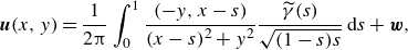 \begin{align} {\boldsymbol{u}}(x,y)=\frac {1}{2 \unicode{x03C0} } \int _0^1 \frac {(- y,x-s)}{(x-s)^2+y^2} \frac {\widetilde {\gamma }(s)}{\sqrt {(1-s)s}} \, \mathrm{d} s + \boldsymbol{w}, \end{align}
where $\boldsymbol{w}$
is a smooth velocity due to free and other bound vorticity in the fluid.
$\boldsymbol{w}$
is a smooth velocity due to free and other bound vorticity in the fluid.
Following Saffman (Reference Saffman1995, p. 98), the suction force is calculated by integrating the Euler momentum equation in a small disk $B_\epsilon$
of radius
$B_\epsilon$
of radius $\epsilon \ll 1$
about the leading edge
$\epsilon \ll 1$
about the leading edge $(x,y)=(0,0)$
:
$(x,y)=(0,0)$
:
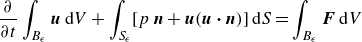 \begin{align} \frac {\partial }{\partial t} \int _{B_\epsilon } {\boldsymbol{u}} \, \mathrm{d} V + \int _{S_\epsilon } [p \, \boldsymbol{n} + {\boldsymbol{u}}({\boldsymbol{u}} \boldsymbol{\cdot} \boldsymbol{n})] \, \mathrm{d} S &= \int _{B_\epsilon } \boldsymbol{F} \, \mathrm{d} V \end{align}
 \begin{align} &= -T \boldsymbol{\hat {i}}, \end{align}
where $p$
is the pressure,
$p$
is the pressure, $\boldsymbol{n}$
is the outward unit normal to the surface
$\boldsymbol{n}$
is the outward unit normal to the surface $S_\epsilon$
of
$S_\epsilon$
of $B_\epsilon$
, and
$B_\epsilon$
, and $\boldsymbol{F}=-T\, \delta ({\boldsymbol{x}})\, \boldsymbol{\hat {i}}$
is the external force, i.e. the force that the leading edge of the wing exerts on the fluid. The suction force of the fluid on the wing is then
$\boldsymbol{F}=-T\, \delta ({\boldsymbol{x}})\, \boldsymbol{\hat {i}}$
is the external force, i.e. the force that the leading edge of the wing exerts on the fluid. The suction force of the fluid on the wing is then $T \boldsymbol{\hat {i}}$
. Here, we have taken the fluid density to be 1. The pressure can be eliminated using Bernoulli’s law (Saffman Reference Saffman1995, p. 19)
$T \boldsymbol{\hat {i}}$
. Here, we have taken the fluid density to be 1. The pressure can be eliminated using Bernoulli’s law (Saffman Reference Saffman1995, p. 19)
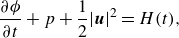 \begin{align} \frac {\partial \phi }{\partial t} +p +\frac {1}{2} |{\boldsymbol{u}}|^2=H(t), \end{align}
where $\phi$
is the velocity potential, and
$\phi$
is the velocity potential, and $H(t)$
is an arbitrary function of time. Multiply (A4) by
$H(t)$
is an arbitrary function of time. Multiply (A4) by $\boldsymbol{n}$
and take the surface integral over
$\boldsymbol{n}$
and take the surface integral over $S_\epsilon$
to obtain at leading order
$S_\epsilon$
to obtain at leading order
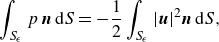 \begin{align} \int _{S_\epsilon } p\, \boldsymbol{n} \, \mathrm{d} S= - \frac {1}{2} \int _{S_\epsilon } |{\boldsymbol{u}}|^2 \boldsymbol{n} \, \mathrm{d} S, \end{align}
where we have neglected terms that are less singular at the plate’s leading edge and thus give higher-order contributions in $\epsilon$
. Substitute (A5) into (A3), and note that the volume integral
$\epsilon$
. Substitute (A5) into (A3), and note that the volume integral $({\partial }/{\partial t}) \int _{B_\epsilon } {\boldsymbol{u}} \, {\rm d}V$
gives a higher-order contribution in
$({\partial }/{\partial t}) \int _{B_\epsilon } {\boldsymbol{u}} \, {\rm d}V$
gives a higher-order contribution in $\epsilon$
, to obtain
$\epsilon$
, to obtain
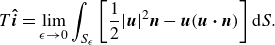 \begin{align} T \boldsymbol{\hat {i}} = \lim _{\epsilon \rightarrow 0} \int _{S_\epsilon } \left [ \frac {1}{2} |{\boldsymbol{u}}|^2 \boldsymbol{n} - {\boldsymbol{u}}({\boldsymbol{u}} \boldsymbol{\cdot} \boldsymbol{n}) \right] \mathrm{d} {S}. \end{align}
We now calculate the velocity at leading order in $\epsilon$
for
$\epsilon$
for $(x,y) \in B_\epsilon$
. In (A1), make the change of variable
$(x,y) \in B_\epsilon$
. In (A1), make the change of variable $-v=x-s$
and expand
$-v=x-s$
and expand $\tilde {\gamma }(x+v)=\tilde {\gamma }(x)+\tilde {\gamma }^{\prime}(x)\, v + \cdots$
to obtain, for
$\tilde {\gamma }(x+v)=\tilde {\gamma }(x)+\tilde {\gamma }^{\prime}(x)\, v + \cdots$
to obtain, for $\boldsymbol{u}=(u_1,u_2)$
,
$\boldsymbol{u}=(u_1,u_2)$
,
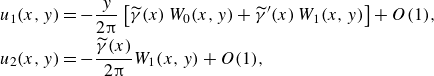 \begin{align} \begin{split} u_1 (x,y)&=- \frac {y}{2 \unicode{x03C0} } \left [\widetilde {\gamma }(x)\, W_0(x,y) +\widetilde {\gamma }^{\prime}(x)\, W_1(x,y) \right]+ O(1), \\ u_2(x,y) &= -\frac {\widetilde {\gamma }(x)}{2 \unicode{x03C0} } W_1(x,y)+O(1), \end{split} \end{align}
where
 \begin{align} \begin{split} W_0(x,y)&= \int _{-x}^{1-x} \frac {1}{(v^2+y^2) \sqrt {(1-(v+x))(v+x)}} \, \mathrm{d} v,\\ W_1(x,y)&= \int _{-x}^{1-x} \frac {v}{(v^2+y^2) \sqrt {(1-(v+x))(v+x)}} \, \mathrm{d} v,\\ \end{split} \end{align}
and the $O(1)$
remainder in (A7) refers to terms for which the Birkhoff–Rott kernel is integrable in
$O(1)$
remainder in (A7) refers to terms for which the Birkhoff–Rott kernel is integrable in $v$
as
$v$
as $y \rightarrow 0$
. The integrals in (A8) can be evaluated in closed form. Let
$y \rightarrow 0$
. The integrals in (A8) can be evaluated in closed form. Let $F(x,y)=\sqrt {(1-x)^2+y^2}$
and
$F(x,y)=\sqrt {(1-x)^2+y^2}$
and $G(x,y)=\sqrt {x^2+y^2}$
. Then (Geer & Keller Reference Geer and Keller1968)
$G(x,y)=\sqrt {x^2+y^2}$
. Then (Geer & Keller Reference Geer and Keller1968)
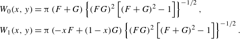 \begin{align} \begin{split} W_0 (x,y)&=\unicode{x03C0} \left ( F+G \right) \left \{ (FG)^2 \left [ (F+G)^2-1 \right] \right \}^{-1/2},\\ W_1 (x,y)&=\unicode{x03C0} \left ( -x F+(1-x) G \right) \left \{ (FG)^2 \left [ (F+G)^2-1 \right] \right \}^{-1/2}. \end{split} \end{align}
Evaluation of (A9) for $x=\epsilon \cos \theta, \ y=\epsilon \sin \theta$
on
$x=\epsilon \cos \theta, \ y=\epsilon \sin \theta$
on $S_\epsilon$
gives, to leading order in
$S_\epsilon$
gives, to leading order in $\epsilon$
,
$\epsilon$
,
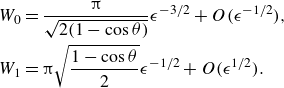 \begin{align} \begin{split} W_0 &= \frac {\unicode{x03C0} }{\sqrt {2(1-\cos \theta)}} \epsilon ^{-3/2} +O(\epsilon ^{-1/2}),\\ W_1 &=\unicode{x03C0} \sqrt {\frac {1-\cos \theta }{2}} \epsilon ^{-1/2}+O(\epsilon ^{1/2}). \end{split} \end{align}
From (A7) and (A10), the leading-order velocity components on $S_\epsilon$
are
$S_\epsilon$
are
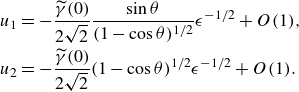 \begin{align} \begin{split} u_1&=- \frac {\widetilde {\gamma }(0)}{2 \sqrt {2}} \frac {\sin \theta }{(1-\cos \theta)^{1/2}} \epsilon ^{-1/2}+ O(1),\\ u_2&= - \frac {\widetilde {\gamma }(0)}{2 \sqrt {2}} (1-\cos \theta)^{1/2} \epsilon ^{-1/2}+ O(1). \end{split} \end{align}
The surface integral in the expression for the suction force can now be computed by substituting (A11) and $\boldsymbol{n}=(\cos \theta, \sin \theta)$
into (A6). We find that the
$\boldsymbol{n}=(\cos \theta, \sin \theta)$
into (A6). We find that the $y$
-component of the suction force is zero as expected, while the
$y$
-component of the suction force is zero as expected, while the $x$
-component satisfies
$x$
-component satisfies
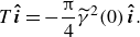 \begin{align} T \boldsymbol{\hat {i}} = -\frac {\unicode{x03C0} }{4} \widetilde {\gamma }^2(0)\, \boldsymbol{\hat {i}}. \end{align}
More generally, the magnitude of the suction force for a horizontal plate with leading edge located at $\boldsymbol{x}$
is
$\boldsymbol{x}$
is
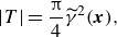 \begin{align} |T| = \frac {\unicode{x03C0} }{4} \widetilde {\gamma }^2(\boldsymbol{x}), \end{align}
with the force oriented in the negative $x$
direction when the leading edge of the wing is located on the left, and in the positive
$x$
direction when the leading edge of the wing is located on the left, and in the positive $x$
direction when the leading edge is on the right.
$x$
direction when the leading edge is on the right.
Appendix B. Comparison between unsteady and steady flow around a vertically translating flat plate
A simple argument for steady flow past a plate, as considered by Acheson (Reference Acheson1990, p. 153), gives results consistent with those of Appendix A. Consider a plate of length $4a$
placed at
$4a$
placed at $x\in [-2a,2a]$
, aligned horizontally with the
$x\in [-2a,2a]$
, aligned horizontally with the $x$
-axis, moving with velocity
$x$
-axis, moving with velocity $(U,V)$
in an inviscid fluid at rest at infinity. Since the horizontal component does not impact thrust, we set
$(U,V)$
in an inviscid fluid at rest at infinity. Since the horizontal component does not impact thrust, we set $U=0$
. Here, we derive the leading-edge normalised sheet strength and leading-edge suction for steady plate motion with singular flow at the leading edge (at
$U=0$
. Here, we derive the leading-edge normalised sheet strength and leading-edge suction for steady plate motion with singular flow at the leading edge (at $z=2a$
), and smooth flow satisfying the Kutta condition at the trailing edge (at
$z=2a$
), and smooth flow satisfying the Kutta condition at the trailing edge (at $z=-2a$
). The steady flow in a reference frame moving with the plate is obtained by the conformal map from the unit circle
$z=-2a$
). The steady flow in a reference frame moving with the plate is obtained by the conformal map from the unit circle $|\zeta |=a$
onto the plate on the
$|\zeta |=a$
onto the plate on the $x$
-axis with
$x$
-axis with $x\in [-2a,2a]$
:
$x\in [-2a,2a]$
:
 \begin{equation} z=J(\zeta)=\zeta +\frac {a^2}{\zeta },\quad \hbox{with}\ \zeta =J^{-1}(z)= \frac {1}{2}\left (z+\sqrt {z^2-4a^2}\right). \end{equation}
Potential flow around the circle with circulation $\Gamma$
is given by the complex potential
$\Gamma$
is given by the complex potential
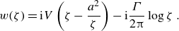 \begin{equation} w(\zeta)=\mathrm{i} V\left (\zeta -\frac {a^2}{\zeta }\right)-\mathrm{i}\frac {\Gamma }{2\unicode{x03C0} }\log \zeta \,. \end{equation}
The complex potential in the $z$
-plane is
$z$
-plane is $W(z)=w(J^{-1}(z))$
, with complex velocity
$W(z)=w(J^{-1}(z))$
, with complex velocity
 \begin{equation} \frac {\mathrm{d} W}{\mathrm{d} z}=\frac {\mathrm{d} w/\mathrm{d} \zeta }{\mathrm{d} z/\mathrm{d} \zeta } =\mathrm{i} V\left (1+\frac {a^2}{\zeta ^2}-\frac {\Gamma }{2\unicode{x03C0} V\zeta }\right) \frac {1}{1-{a^2}/{\zeta ^2}} =\frac {\mathrm{i} V}{\zeta ^2-a^2}\left (\zeta ^2 -\frac {\Gamma }{2\unicode{x03C0} V}\zeta + a^2\right). \end{equation}
The singularity at the trailing edge $z=-2a$
(
$z=-2a$
( $\zeta =-a$
) is removed by setting
$\zeta =-a$
) is removed by setting
 \begin{equation} \Gamma =-4\unicode{x03C0} V a\,, \end{equation}
so that
 \begin{equation} \frac {\mathrm{d} W}{\mathrm{d} z}= \mathrm{i} V\frac {\zeta +a}{\zeta -a}\,. \end{equation}
The resulting velocity on the plate is obtained by setting $\zeta =a\,{\rm e}^{\mathrm{i} \theta }\ (x=2a\cos \theta)$
, where
$\zeta =a\,{\rm e}^{\mathrm{i} \theta }\ (x=2a\cos \theta)$
, where $\theta \in [0,\unicode{x03C0}]$
corresponds to the top of the plate, and
$\theta \in [0,\unicode{x03C0}]$
corresponds to the top of the plate, and $\theta \in [\unicode{x03C0}, 2\unicode{x03C0}]$
to the bottom:
$\theta \in [\unicode{x03C0}, 2\unicode{x03C0}]$
to the bottom:
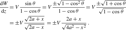 \begin{equation} \begin{aligned} \frac {\mathrm{d} W}{\mathrm{d} z} &=V\frac {\sin \theta } {1-\cos \theta } =V\frac {\pm \sqrt {1-\cos ^2\theta }} {1-\cos \theta } =V\frac {\pm \sqrt {1+\cos \theta }} {\sqrt {1-\cos \theta }}\\ &=\pm V\frac {\sqrt {2a+x}}{\sqrt {2a-x}}\, =\pm V\frac {2a+x}{\sqrt {4a^2-x^2}}\,. \end{aligned} \end{equation}
For positive $V$
, the top velocity is positive and the bottom is negative. This yields the vortex sheet strength
$V$
, the top velocity is positive and the bottom is negative. This yields the vortex sheet strength
 \begin{equation} \gamma (x) = u_{-}-u_{+}=-2V\frac {2a+x}{\sqrt {4a^2-x^2}} =-2V\frac {2a+x}{\sqrt {4a^2-x^2}} =\frac {\widetilde {\gamma }(x)}{\sqrt {4a^2-x^2}}, \end{equation}
where $\widetilde {\gamma }(x)=\gamma (x) {\sqrt {4a^2-x^2}}$
. This definition of
$\widetilde {\gamma }(x)=\gamma (x) {\sqrt {4a^2-x^2}}$
. This definition of $\widetilde {\gamma }$
is consistent with (A1) with
$\widetilde {\gamma }$
is consistent with (A1) with $s=x+1/2,\ a=1/4$
, and (2.6) with
$s=x+1/2,\ a=1/4$
, and (2.6) with $s=x, a=1/4$
. For
$s=x, a=1/4$
. For $a=1/4$
, the leading-edge normalised sheet strength is
$a=1/4$
, the leading-edge normalised sheet strength is $\widetilde {\gamma }(1/2)=-2V$
.
$\widetilde {\gamma }(1/2)=-2V$
.
Using Blasius’ theorem, we find that the total force on the plate is
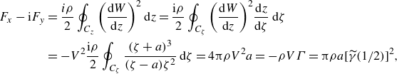 \begin{equation} \begin{aligned} F_x-\mathrm{i} F_y &=\frac {i\rho }{2}\oint _{C_z}{\left (\frac {\mathrm{d} W}{\mathrm{d} z}\right)}^2\,\mathrm{d} z =\frac {\mathrm{i}\rho }{2}\oint _{C_\zeta }{\left (\frac {\mathrm{d} W}{\mathrm{d} z}\right)}^2\frac {\mathrm{d} z}{\mathrm{d}\zeta }\,\mathrm{d}\zeta \\ &=-V^2\frac {\mathrm{i}\rho }{2}\oint _{C_\zeta }\frac {(\zeta +a)^3}{(\zeta -a)\zeta ^2}\,\mathrm{d}\zeta =4\unicode{x03C0} \rho V^2a =-\rho V\Gamma =\unicode{x03C0} \rho a [\widetilde {\gamma }(1/2)]^2, \end{aligned} \end{equation}
picking up the residues at $\zeta =0,a$
. Expression (B8) is consistent with (A13) by setting
$\zeta =0,a$
. Expression (B8) is consistent with (A13) by setting $\rho =1$
,
$\rho =1$
, $a=1/4$
.
$a=1/4$
.


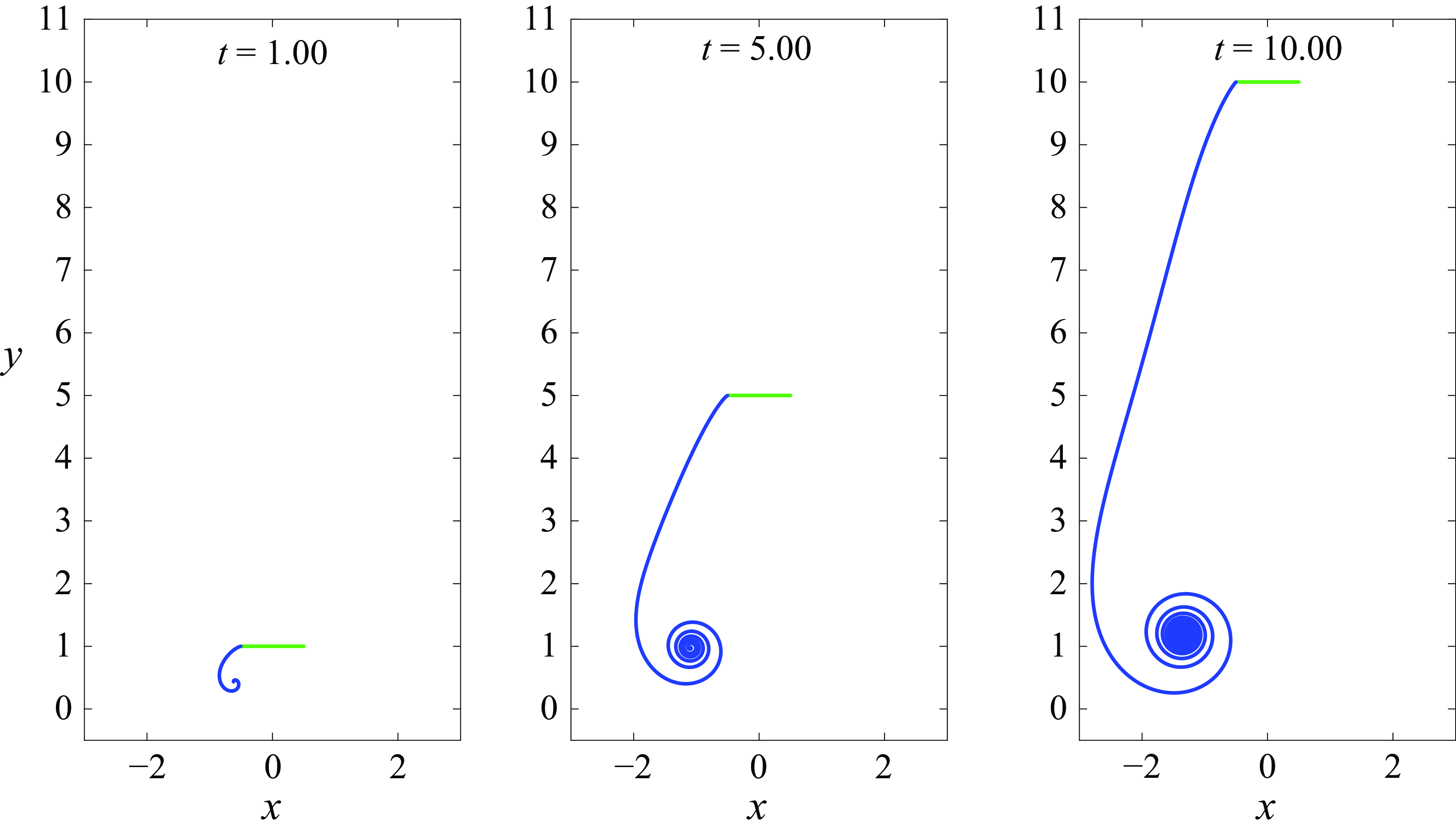
Figure 13. Impulsively started plate that translates vertically with constant velocity $V=1$
, and the vortex sheet that separates from its left-hand endpoint, shown at the indicated times.
$V=1$
, and the vortex sheet that separates from its left-hand endpoint, shown at the indicated times.
Figure 12 shows the streamlines of the resulting steady flow past the plate with $V=1$
and
$V=1$
and $a=1/4$
, in a reference frame moving with the plate, where the circulation given by (B4) cancels the singularity at the trailing (left-hand) edge. Note the resulting stagnation point at the trailing edge and the symmetry across
$a=1/4$
, in a reference frame moving with the plate, where the circulation given by (B4) cancels the singularity at the trailing (left-hand) edge. Note the resulting stagnation point at the trailing edge and the symmetry across $y=0$
.
$y=0$
.
We now consider an impulsively started plate with $a=1/4$
, initially on the
$a=1/4$
, initially on the $x$
-axis and centred at the origin, moving vertically upwards with constant velocity
$x$
-axis and centred at the origin, moving vertically upwards with constant velocity $V=1$
for
$V=1$
for $t\gt 0$
. The singularity at the left-hand edge is resolved by satisfying the Kutta condition through vortex sheet generation and separation via the method described in § 2. Figure 13 shows the position of the plate and the separated vortex sheet at a sequence of times.
$t\gt 0$
. The singularity at the left-hand edge is resolved by satisfying the Kutta condition through vortex sheet generation and separation via the method described in § 2. Figure 13 shows the position of the plate and the separated vortex sheet at a sequence of times.
Figure 14 shows the corresponding streamlines, in a reference frame moving with the plate. It shows that as $t\to \infty$
, the flow approaches the steady symmetric potential flow discussed above and shown in figure 12. Furthermore, note the position of the stagnation point on the upper plate side. Initially, the impulsively started flow is symmetric, with a stagnation point at the middle of the plate at
$t\to \infty$
, the flow approaches the steady symmetric potential flow discussed above and shown in figure 12. Furthermore, note the position of the stagnation point on the upper plate side. Initially, the impulsively started flow is symmetric, with a stagnation point at the middle of the plate at $x=0$
. As time evolves, the unsteady flow approaches the steady flow configuration, and the stagnation point moves progressively closer to the trailing edge.
$x=0$
. As time evolves, the unsteady flow approaches the steady flow configuration, and the stagnation point moves progressively closer to the trailing edge.
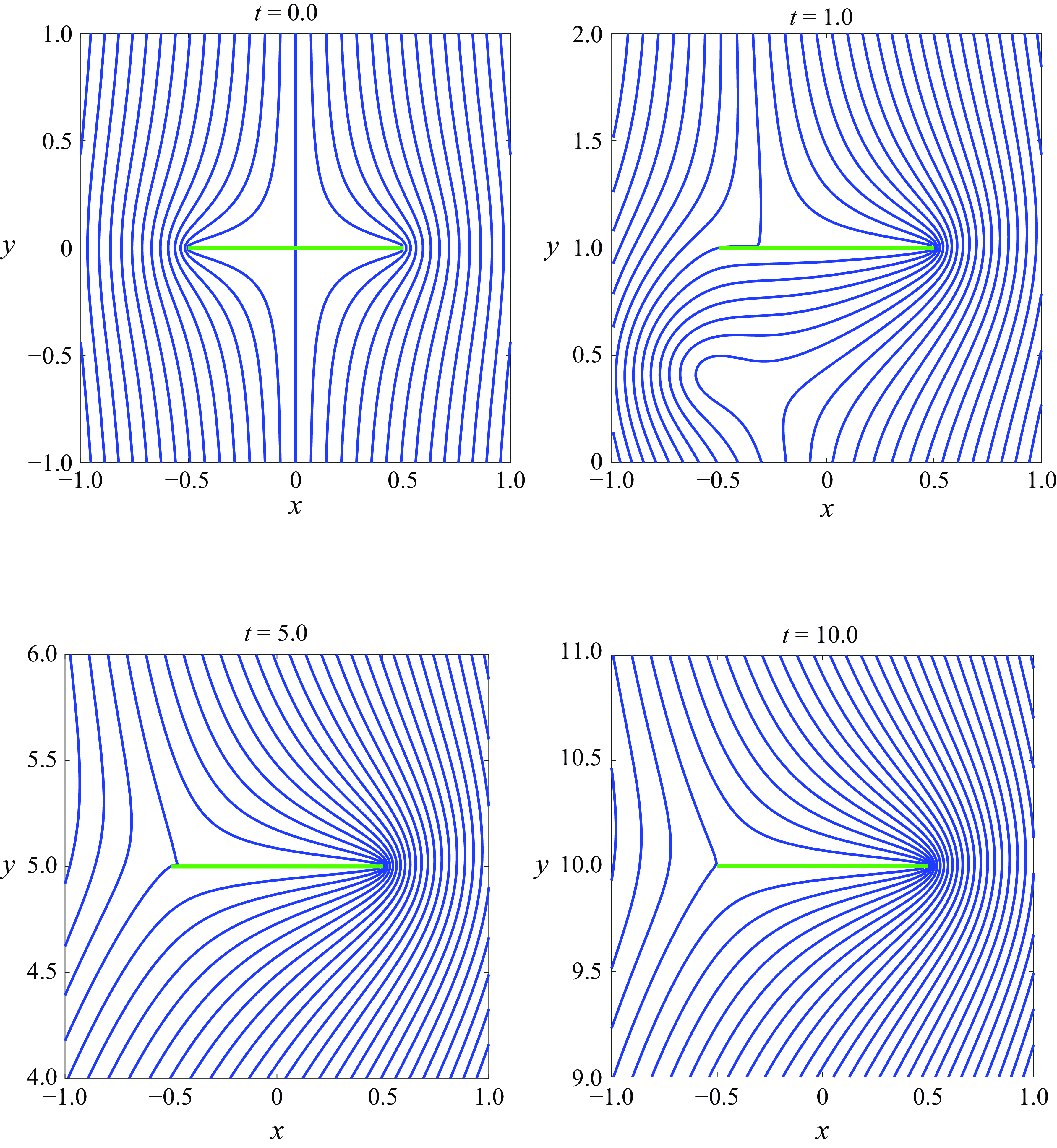
Figure 14. Streamlines of the flow in figure 13, shown in a reference frame moving with the plate.
Figure 15 shows the desingularised leading-edge sheet strength and the circulation about the plate for the impulsively started plate. Note that the total circulation about the plate and the shed vortex sheet is enforced to stay constant at zero. The plate circulation is thus the negative of the circulation in the shed vortex sheet. The figure shows that both the shed sheet strength and the plate circulation approach the steady-state values as $t\to \infty$
, with
$t\to \infty$
, with $\widetilde {\gamma }\to -2V$
and
$\widetilde {\gamma }\to -2V$
and $\Gamma \to -\unicode{x03C0} V$
.
$\Gamma \to -\unicode{x03C0} V$
.
These numerical results illustrate the difference between steady and unsteady flow, and provide further consistency between the steady-state results derived here and the unsteady results derived in Appendix A.
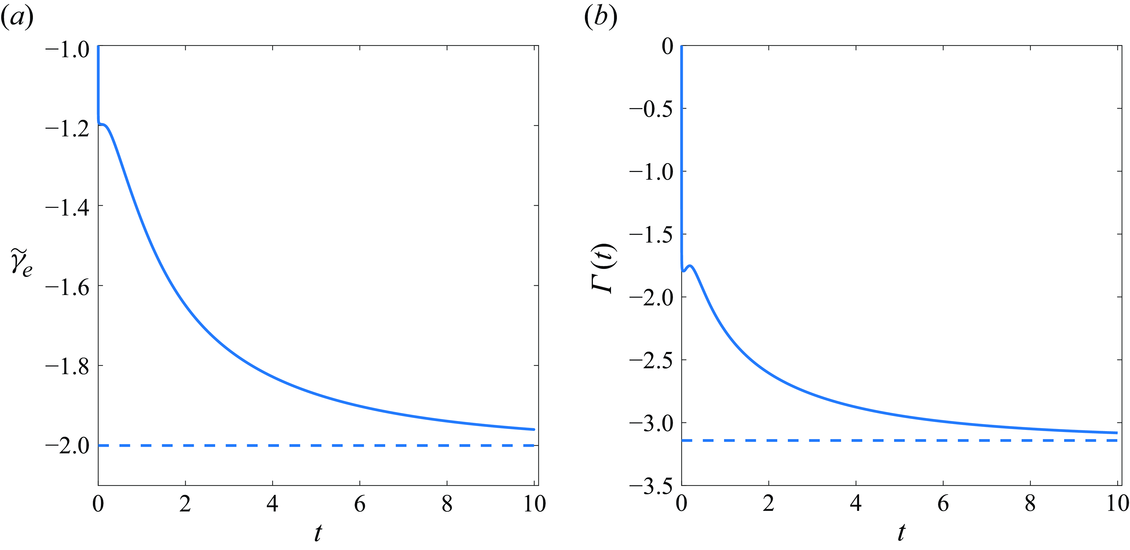
Figure 15. (a) Desingularised leading-edge sheet strength $\widetilde {\gamma }(1/2)$
, and (b) total circulation around the plate
$\widetilde {\gamma }(1/2)$
, and (b) total circulation around the plate $\Gamma (t)$
, corresponding to the flow in figure 13.
$\Gamma (t)$
, corresponding to the flow in figure 13.
Appendix C. Alternative model for the drag force acting on the plates
To compute the drag on plate $j$
, we simply use the plate velocity
$j$
, we simply use the plate velocity $U^j$
, which induces drag relative to the stagnant background flow. An alternative model that better accounts for the horizontal velocity above and below the plate, used by Fang (Reference Fang2016) and Heydari & Kanso (Reference Heydari and Kanso2021), is obtained by replacing
$U^j$
, which induces drag relative to the stagnant background flow. An alternative model that better accounts for the horizontal velocity above and below the plate, used by Fang (Reference Fang2016) and Heydari & Kanso (Reference Heydari and Kanso2021), is obtained by replacing
 \begin{equation} C_d(U^j)^{3/2} \end{equation}
in (2.11b ) by
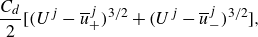 \begin{equation} \frac {C_d}{2} [ (U^j-\overline {u}_+^j)^{3/2} + (U^j-\overline {u}_-^j)^{3/2}], \end{equation}
where
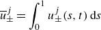 \begin{equation} \overline {u}_{\pm }^j=\int _0^1 u_{\pm }^j(s,t) \,\mathrm{d}s \end{equation}
are the average horizontal velocities just above and below the plate, and $u_{\pm }^j(s,t)$
are the limiting horizontal velocities from above and below the plate, respectively. Equation (C2) assumes that
$u_{\pm }^j(s,t)$
are the limiting horizontal velocities from above and below the plate, respectively. Equation (C2) assumes that $U^j-\overline {u}_{\pm }^j\gt 0$
, which is the case in the present paper.
$U^j-\overline {u}_{\pm }^j\gt 0$
, which is the case in the present paper.
The velocities $u^j_{\pm }(s)$
have two components, one stemming from the
$u^j_{\pm }(s)$
have two components, one stemming from the $j$
th plate, and one stemming from the far-field vorticity in all the other
$j$
th plate, and one stemming from the far-field vorticity in all the other $n-1$
plates and all the
$n-1$
plates and all the $n$
wakes:
$n$
wakes:
 \begin{equation} u^j_{\pm }= u^j_{\pm \textit{plate}} +u^j_{\textit{far}}\,. \end{equation}
The average of this sum is the sum of the average of each component.
The first component is discontinuous across the plate. Note that the jump in the horizontal velocity across the plate equals the negative sheet strength, and the average of the horizontal velocities above and below the plate, induced by itself, is zero:
 \begin{align} u^j_{+\textit{plate}} -u^j_{-\textit{plate}}&=-\gamma (s,t)\,, \end{align}
 \begin{align} \frac {1}{2}\left (u^j_{+\textit{plate}} +u^j_{-\textit{plate}}\right)&=0\,, \end{align}
thus
 \begin{equation} u^j_{+\textit{plate}} =-\gamma (s)/2\,,\quad u^j_{-\textit{plate}} =+\gamma (s)/2\,. \end{equation}
As a result,
 \begin{equation} \overline {u}^j_{\pm \textit{plate}} =\mp \frac {1}{2}\int _0^1\gamma (s)\,\mathrm{d}s=\pm \frac {1}{2}\Gamma_T^j. \end{equation}
The last equality follows since the total circulation about each plate is the negative of the shed vorticity $\Gamma_T^j$
.
$\Gamma_T^j$
.
Furthermore, note that if $\Gamma_T^j/2\lt U^j$
, then the contribution of this self-induced term to the difference between (C2) and (C1) is of order
$\Gamma_T^j/2\lt U^j$
, then the contribution of this self-induced term to the difference between (C2) and (C1) is of order
 \begin{equation} C_d\frac {3}{4}\left (\frac {\Gamma_T^j}{2U^j}\right)^2, \end{equation}
so is excepted to be small. Indeed, we observe in our simulations that $\Gamma ^T/2U\leqslant 0.4$
for the amplitudes
$\Gamma ^T/2U\leqslant 0.4$
for the amplitudes $A=0.1{-}0.4$
that we considered, so the contribution (C8) is expected to be
$A=0.1{-}0.4$
that we considered, so the contribution (C8) is expected to be $\leqslant 2\%$
for
$\leqslant 2\%$
for $C_d=0.1$
.
$C_d=0.1$
.
The second component, the far-field contribution $u^j_{\mathrm{far}}$
to
$u^j_{\mathrm{far}}$
to $u^j_{\pm }(s,t)$
, is continuous across the
$u^j_{\pm }(s,t)$
, is continuous across the $j$
th plate. It consists of only the contribution of the free vorticity in all
$j$
th plate. It consists of only the contribution of the free vorticity in all $n$
wakes, and not any bound plate vorticity. The reason the other
$n$
wakes, and not any bound plate vorticity. The reason the other $n-1$
plates do not contribute to the horizontal velocity on the
$n-1$
plates do not contribute to the horizontal velocity on the $j$
th plate is that they are positioned in line with the
$j$
th plate is that they are positioned in line with the $j$
th plate. We compute
$j$
th plate. We compute $u^j_{\mathrm{far}}$
by evaluating the horizontal component of
$u^j_{\mathrm{far}}$
by evaluating the horizontal component of
 \begin{equation} \boldsymbol{u}(\boldsymbol{x}_o,t) = \frac {1}{2\unicode{x03C0} }\sum _{l=1}^n \int _0^{\Gamma _T^l} \frac {(\boldsymbol{x}_o-\boldsymbol{x}_f^l(\Gamma,t))^{\perp }} {|\boldsymbol{x}_o-\boldsymbol{x}_f^l(\Gamma,t)|^2+\delta ^2}\,\textrm {d}\Gamma \end{equation}
at all midpoints $\boldsymbol{x}_o=\boldsymbol{x}^j(\alpha _k^m)$
, then using the midpoint rule to obtain
$\boldsymbol{x}_o=\boldsymbol{x}^j(\alpha _k^m)$
, then using the midpoint rule to obtain
 \begin{align} \overline {u}^j_{\mathrm{far}}=\sum _{k=0}^n u(\boldsymbol{x}^j(\alpha _k^m))\,s^{\prime}(\alpha _k^m)\,(\alpha _{k}-\alpha _{k-1})\,. \end{align}
This second component is expected to be small for a single plate ( $n=1$
), since the wake is behind the plate. It is expected to be less negligible for
$n=1$
), since the wake is behind the plate. It is expected to be less negligible for $n\gt 1$
plates, when the
$n\gt 1$
plates, when the $j$
th plate is in the wake of the upstream plates.
$j$
th plate is in the wake of the upstream plates.
As a result, we expect the change introduced by the alternative model (C2) over the simple model (C1) to be small if $n=1$
, thus it will not significantly affect the steady-state velocity if
$n=1$
, thus it will not significantly affect the steady-state velocity if $n=1$
. For
$n=1$
. For $n\gt 1$
, the rear plates have been shown to have small impact on the first plate. Since at steady state all plates travel at the same speed, the steady-state velocity for
$n\gt 1$
, the rear plates have been shown to have small impact on the first plate. Since at steady state all plates travel at the same speed, the steady-state velocity for $n\gt 1$
computed with the alternative model is expected to be similar to that in the original model.
$n\gt 1$
computed with the alternative model is expected to be similar to that in the original model.
These conjectures were confirmed by numerical results for sample cases using $A=0.2$
and
$A=0.2$
and $C_d=0.1$
. We computed the translation velocity
$C_d=0.1$
. We computed the translation velocity $U^j$
for
$U^j$
for $n=1$
and
$n=1$
and $n=2$
, and the equilibrium separation distance
$n=2$
, and the equilibrium separation distance $d_1^{\infty,1}$
for
$d_1^{\infty,1}$
for $n=2$
, and found that the translation velocity computed with the alternative drag model decreased by 4 % over the simple model, and the separation distance decreased by 3 %. This shows that there is little difference between the two drag models for the parameter regime considered herein, and changing from one to the other is not expected to change the main conclusions of this paper.
$n=2$
, and found that the translation velocity computed with the alternative drag model decreased by 4 % over the simple model, and the separation distance decreased by 3 %. This shows that there is little difference between the two drag models for the parameter regime considered herein, and changing from one to the other is not expected to change the main conclusions of this paper.


 Open access