


1. Introduction
The stability and transition mechanisms in the adverse pressure gradient (APG) boundary layer have been studied extensively (Brinkerhoff & Yaras Reference Brinkerhoff and Yaras2011; Lambert & Yarusevych Reference Lambert and Yarusevych2019; Sengupta & Tucker Reference Sengupta and Tucker2020), given their frequent appearance in various engineering applications. For instance, the performance of turbo-machines, including pumps, turbines and compressors, is affected adversely by the flow separation occurring from APG conditions (Greenblatt & Wygnanski Reference Greenblatt and Wygnanski2000; Sandberg & Michelassi Reference Sandberg and Michelassi2022). A recent review by Sandberg & Michelassi (Reference Sandberg and Michelassi2022) summarizes the consequences of flow separation and various modelling approaches in axial turbo-machines. During such complex real-world applications involving APG conditions, the boundary layer thickness can vary spatially and temporally, bringing about a set of inflectional velocity profiles at random times and points along the surface, making the investigation difficult.
Historically, separation bubble formation and growth were isolatedly investigated by employing blowing/suction (Alam & Sandham Reference Alam and Sandham2000; Embacher & Fasel Reference Embacher and Fasel2014), spatially varying wall contours (Mariotti et al. Reference Mariotti, Grozescu, Buresti and Salvetti2013), and attaching distinctive shapes to the wall (Wissink & Rodi Reference Wissink and Rodi2006; Garcia-Villalba et al. Reference Garcia-Villalba, Li, Rodi and Leschziner2009). Further, the receptivity analysis is used extensively to delineate the mechanism that amplifies or decays the velocity field disturbances within the boundary layer of laminar and marginally separated flows (Goldstein & Hultgren Reference Goldstein and Hultgren1989; Diwan & Ramesh Reference Diwan and Ramesh2009; Jain, Ruban & Braun Reference Jain, Ruban and Braun2021). These studies demonstrated that the Lambda vortex-induced breakdown of a separated shear layer occurs in short laminar bubbles, and their absolute instability nature. Despite the absence of disturbances upstream, the disintegration produced by separation bubbles was characterized by the evolution of low-frequency oscillations with a high amplitude within itself (Sandham Reference Sandham2008). A time-varying external flow or free-stream turbulence may enhance or reduce an adverse pressure gradient and alter the separation location over time, further complicating the problem. Hence the effect of unsteady inflow conditions on non-uniform channels has been the subject of many studies (Tutty & Pedley Reference Tutty and Pedley1993; Rosenfeld Reference Rosenfeld1995; Wissink, Michelassi & Rodi Reference Wissink, Michelassi and Rodi2004; Wissink & Rodi Reference Wissink and Rodi2006; Das, Srinivasan & Arakeri Reference Das, Srinivasan and Arakeri2013, Reference Das, Srinivasan and Arakeri2016).
Numerical simulations are employed frequently to investigate the effects of periodic external oscillations on separation flow dynamics. In a stepped channel, Tutty & Pedley (Reference Tutty and Pedley1993) analysed the formation and propagation of ‘vortex waves’ generated during an oscillatory flow's forward and backward phase, using two-dimensional simulations. Alternatively, Rosenfeld (Reference Rosenfeld1995) examined the influence of Reynolds number and Strouhal number on vortex formation and propagation in a constricted channel. Wissink & Rodi (Reference Wissink and Rodi2006) investigated the effect of oscillatory flow in transitional separated flow over a smooth converging and diverging section by employing three-dimensional numerical simulations. Wissink et al. (Reference Wissink, Michelassi and Rodi2004) further investigated the heat transfer aspects of a laminar separation bubble affected by the oscillating external flow.
The effects of spatial and temporal pressure gradient conditions on vortex formation and associated instabilities have been extensively examined experimentally under trapezoidal mean flow conditions coupled with various geometrical configurations (Das & Arakeri Reference Das and Arakeri1998; Das et al. Reference Das, Srinivasan and Arakeri2013, Reference Das, Srinivasan and Arakeri2016; Ramalingam & Das Reference Ramalingam and Das2020). Trapezoidal flows, in contrast to pulsating ones, are appropriate for investigating the effects of constant acceleration and deceleration on flow dynamics. Das & Arakeri (Reference Das and Arakeri1998) used a trapezoidal variation of the mean flow created by piston motion to study the instabilities of rapidly decelerating pipe flows. Das et al. (Reference Das, Srinivasan and Arakeri2013) analysed flow structures originating from bluff bodies and critical time scales for similar mean flow conditions. Recently, Ramalingam & Das (Reference Ramalingam and Das2020) performed a detailed visualization study on the flow structures in a water channel flow using direct visualization and particle image velocimetry. Das et al. (Reference Das, Srinivasan and Arakeri2016) conducted a fascinating experimental investigation in a diverging water channel to investigate the transition mechanism in APG conditions. In response to two-dimensional inflectional instabilities, an apparent roll-up of the shear layer is observed in both the lower and upper walls. One crucial experimental observation in their study was the highly localized transition to turbulence of shear layer vortices generated by primary instability.
The stability characteristics of flows with non-zero mean velocity have been the subject of several studies. Through a quasi-steady approach, Hall & Parker (Reference Hall and Parker1976) investigated the growth of the disturbance velocity field associated with the inflectional velocity profiles in a decaying laminar flow. Based on a linear instability analysis of the inflectional velocity profiles generated in an oscillating pipe flow, a relationship between the flow stability and inflection point was posited by Das & Arakeri (Reference Das and Arakeri1998). The wavenumber associated with the highest growth rate for such profiles is nearly constant. Additionally, a linear and weakly nonlinear analysis of a laminar flow subjected to rapid acceleration/deceleration by Ghidaoui & Kolyshkin (Reference Ghidaoui and Kolyshkin2002) reinterprets the stability region predicted by Das & Arakeri (Reference Das and Arakeri1998). Furthermore, it was discovered that the Ginzburg–Landau equation governs the amplitude of the most unstable mode. Using optimal growth analysis of normal modes, Nayak & Das (Reference Nayak and Das2017) provide accurate growth rate predictions for unsteady channel flows. Recently, Kannaiyan, Natarajan & Vinoth (Reference Kannaiyan, Natarajan and Vinoth2022) investigated the stability characteristics of laminar pipe flow with a step-like flow rate increment, by using a linear modal stability framework combined with a quasi-steady assumption.
Multiple researchers have analysed the secondary instability and the transition of shear layer vortices resulting from separated flows (Caulfield & Kerswell Reference Caulfield and Kerswell2000; Jones, Sandberg & Sandham Reference Jones, Sandberg and Sandham2008; Mashayek & Peltier Reference Mashayek and Peltier2012; Zhiyin Reference Zhiyin2019). Shear layer vortices are susceptible to secondary instability in the elliptic and hyperbolic regions (core and braid regions, respectively), resulting in periodic streamwise vortices formation. For example, Mode A and Mode B instabilities in the transitional cylinder wake correspond to hyperbolic and elliptic instability in the wake vortices, respectively (Leweke & Williamson Reference Leweke and Williamson1998). Caulfield & Kerswell (Reference Caulfield and Kerswell2000) described mathematically the braid region instability arising over the hyperbolic stagnation points in mixing layer flows. Jones et al. (Reference Jones, Sandberg and Sandham2008) have confirmed the destabilization of the braid region between vortex structures emerging from a separated flow over the surface of an aerofoil and relate it to the mode-B instability of hyperbolic streamlines in two dimensions; the same is often true for bluff-body wakes.
A study by Abdalla & Yang (Reference Abdalla and Yang2004) demonstrated that the onset of turbulence could be attributed to a helical pairing of spanwise vortex rolls originating from Kelvin–Helmholtz instability. For the vortices shed from laminar separation bubbles, Marxen, Lang & Rist (Reference Marxen, Lang and Rist2013) posited multiple instability mechanisms that lead to turbulent transitions. The first mechanism, identified as elliptical instability, distorts the vortex structure with a spanwise wavelength in the order of the vortex dimension. In contrast, the other instability develops in the braid region with a higher spanwise wavenumber. Recently, by analysing the three-dimensional coherent structures arising in the wake of a wall-attached body, Sarath & Manu (Reference Sarath and Manu2022) showed that the vortices shed from boundary layers displayed simultaneously both elliptical and hyperbolic instability.
Various theoretical models are used to measure the growth rate of vortices associated with secondary instabilities. Rankine vortices and Lamb–Oseen vortex pairs are generally used to approximate vorticity distributions for estimating the theoretical growth rates of primary vortices (Le Dizes Reference Le Dizes2000a). Furthermore, Le Dizes (Reference Le Dizes2000b) developed a growth rate relation by neglecting the viscous effects for a multipolar vortex in a rotating flow field, with estimates comparable to the global instability analysis results for various vorticity distributions such as Kirchhoff (Miyazaki, Imai & Fukumoto Reference Miyazaki, Imai and Fukumoto1995) and Moore and Saffman (Moore & Saffman Reference Moore and Saffman1971) vortices. A consolidated review of Kerswell (Reference Kerswell2002) discusses in detail the emergence of elliptical instability in different flow scenarios. An extended investigation by Le Dizes & Laporte (Reference Le Dizes and Laporte2002) identifies a relation to predict the elliptic instability growth rate in a vortex pair, and establishes a critical region for the Reynolds number based on the circulation. A recent review on the instabilities arising in a vortex pair by Leweke, Le Dizes & Williamson (Reference Leweke, Le Dizes and Williamson2016) proposes a revised estimation of the growth rate for elliptic instability.
The present work examines the flow breakdown mechanism in a decelerating diverging channel through numerical simulation using a flow configuration similar to the experiments of Das et al. (Reference Das, Srinivasan and Arakeri2016). High-fidelity simulations are performed here to determine the evolution of the flow features within a diverging channel with variable inflow velocity, and the three-dimensional aspects of the vortex flow features are identified, which are largely unexplored by Das et al. (Reference Das, Srinivasan and Arakeri2016). By studying velocity profiles, we examine the primary mechanism of instability, while streamwise vorticity analyses are used to study the secondary instability mechanism. The stability of coherent flow features and their temporal characteristics are identified from dynamic mode decomposition (DMD) analysis. Further analyses of the vortex's stability are conducted using theoretical growth rate estimates using the vortex parameters identified from a comparable Lamb–Oseen approximation.
This paper is arranged as follows. Section 2 includes the details about the computational methods, along with the boundary conditions involved, and the validation results obtained via comparison with experimental observations. Section 3 describes the various flow instability traits discovered in three-dimensional simulations, and the details about the classification of cases using streamwise vorticity evolution (type I to type III). Vortex flow evolution characteristics in categories type I, type II and type III are provided in §§ 4, 5, and 6, respectively. Section 7 summarizes the observed flow dynamics and instability analysis results.
2. Numerical methodology
2.1. Governing equations
The time-dependent three-dimensional flow field is obtained by solving the following governing equations. The continuity and momentum equations for a three-dimensional, incompressible and viscous flow are given as
 \begin{equation} \left.\begin{gathered} \boldsymbol{\nabla}\boldsymbol{\cdot} \boldsymbol{V} = 0, \\ \frac{\partial \boldsymbol{V}}{\partial t} =-\boldsymbol{\nabla} p -\frac{1}{2} \left[\boldsymbol{\nabla}(\boldsymbol{V}\otimes \boldsymbol{V}) + (\boldsymbol{V}\boldsymbol{\cdot}\boldsymbol{\nabla})\boldsymbol{V} \right]+\nu\, \nabla^2\boldsymbol{V} +f. \end{gathered}\right\} \end{equation}
 In the above equation,  $\boldsymbol {V}$ is the velocity vector with components $u$,
$u$,  $v$ and $w$ in the streamwise, wall-normal and spanwise directions, respectively. Here, $t$,
$t$,  $p$ and $\nu$ correspond to flow time, pressure and kinematic viscosity. The nonlinear terms in the governing equation are expressed in the skew-symmetric form since it is resilient to aliasing errors (Kravchenko & Moin Reference Kravchenko and Moin1997). The embedded body region in the computational domain is enforced by the body force field ( $\,f$) in the momentum equation using the immersed boundary method (IBM). For numerically solving the governing equations, a high-order finite-difference flow solver Incompact3d (Laizet & Lamballais Reference Laizet and Lamballais2009; Laizet & Li Reference Laizet and Li2011), with a Cartesian mesh, is used. Incompact3d has been used extensively for various transitional and turbulent flow studies (Bempedelis & Steiros Reference Bempedelis and Steiros2022; Giri et al. Reference Giri, Biswas, Chase, Xue, Abkarian, Mendez, Saha and Stone2022).
In this code, spatial discretization of governing equations on a uniformly spaced Cartesian mesh is accomplished using a sixth-order compact finite-difference scheme. A third-order Adams–Bashforth approach is used for the time integration of the discretized governing equation. A staggered pressure grid from the velocity grid by half mesh length is implemented to avoid spurious pressure oscillations. The modified Poisson equation obtained by imposing the IBM is dealt with by spectral methods using the modified wavenumber formalism. 2Decomp&FFT (Li & Laizet Reference Li and Laizet2010), a domain decomposition library, performs fast Fourier transforms involved in spectral techniques. The library also contains a domain decomposition algorithm for efficient scaling and distribution of memory in high-performance computing systems.
2.2. Computational domain and boundary conditions
A sketch of the computational set-up of flow in a diverging channel is shown in figure 1. The computational domain chosen for this study is a small segment of the experimental set-up employed by Das et al. (Reference Das, Srinivasan and Arakeri2016). Here,  $X$,
$X$,  $Y$ and $Z$ are streamwise, wall-normal and spanwise distances, respectively. In the simulation, the computational domain has length 1.2 m, width 0.142 m, which is equal to half the width of the experimental section, and height 0.15 m, as illustrated in figure 1(a). At the constant channel section, the embedded body section has height 0.07 m. After a length 0.3464 m, the edge starts to curve along an arc with radius (R) 0.1 m. Later, the curve joins smoothly to the diverging section with angle of depression $6.2 ^\circ$ (figure 1b). Similarly, the end of the diverging part joins fluidly with the bottom wall of the channel.

Figure 1. Computational domain along with boundary conditions: (a) three-dimensional view of the computational domain; (b) dimensions of the diverging section; (c) mean inflow variation during a pulse; and (d) variations in the inlet velocity profile during different velocity phases. (All the dimensions are in metres.)
A no-slip boundary condition is enforced on both top and bottom walls for devising identical experimental set-up conditions in the computational domain. A time-varying inlet condition based on the analytical solution of trapezoidal mean flow variation is imposed at the inlet of the computational domain. The free-slip condition is applied to both the right and left boundaries. The one-dimensional advective outflow equation is implemented as the exit boundary condition is given by
 \begin{equation} \left.\frac{\partial u}{\partial t} \right|_{{X}=l_x} + U_c \left.\frac{\partial u}{\partial {X}}\right|_{{X}=l_x} = 0, \end{equation}
where the mean velocity of the inlet velocity profile is taken as the advection velocity ( $U_c$), and $l_x$ is the domain length in the streamwise direction.
The following equations give the mean inflow velocity for the four phases of piston motion:
 \begin{align} u_{p}(t)&=U_{p}\,\frac{t}{t_0 } \quad \text{for} \ 0\leq t\leq t_0, \nonumber\\ &=U_{p} \quad \text{for} \ t_0\leq t\leq t_1, \nonumber\\ &=U_{p}\,\frac{t_2-t}{t_2-t_1}\quad \text{for} \ t_1\leq t\leq t_2, \nonumber\\ &=0\quad \text{for} \ t> t_2. \end{align}
 A trapezoidal pulse of mean inflow constitutes a constant acceleration phase ( $0$ to $t_0$), a constant mean inflow phase ( $t_0$ to $t_1$), and a constant deceleration phase ( $t_1$ to $t_2$). Here, $U_p$ is the mean inlet velocity in the constant inflow phase (figure 1c). Such an inflow configuration can study the individual effects of the acceleration and deceleration phases of the inflow pulse. Analytical solutions of a trapezoidal mean inflow variation (2.3) for a two-dimensional channel following Das & Arakeri (Reference Das and Arakeri1998) are imposed at the inlet. Time-varying small-amplitude perturbations are generated by the combination of two parts of the analytical velocity solution (A5). The inlet boundary condition is not modified to account for free-stream turbulence. Details on the governing equations and solution procedures, along with velocity profiles imposed at the inlet during different phases, can be found in Appendix A. This approach shortens the entrance length and allows a shorter domain, reducing computational load. Since the inlet velocity profiles are built upon the assumption of a two-dimensional channel, using a subdomain guarantees the application of a slip boundary on the sidewalls. The work of Sarath & Manu (Reference Sarath and Manu2022) provides additional information about the procedure to obtain the inflow velocity profile.
Four typical velocity profiles imposed at the inlet during different phases are shown in figure 1(d). The analytical solution generates oscillating components, which cause small-amplitude oscillations, as shown in the figure. The amplitude of oscillations depends on the phase of the mean inflow velocity, and decreases when the mean inflow velocity is constant, as shown in instances V2 and V4. A spanwise width 0.142 m is sufficient to allow the domain to accommodate spanwise oscillations formed by the three-dimensional instability. Keeping the same channel height while reducing the area under consideration in the streamwise and spanwise directions allows for denser grid analysis and minimizes the computational load. A complete domain simulation demonstrated minor deviations (less than 1 %) in the wavelength of spanwise oscillation, affirming the selection of such a section for numerical analysis.
In the remaining sections of this paper, flow features are illustrated using non-dimensional spatial scales. Streamwise distance is non-dimensionalized as  $x = ({X - X_s})/{h_b}$, where $h_b$ is the embedded body height at the inlet, and $X_s$ denotes the start of the diverging section ( $X_s = 0.3464$). Wall-normal and spanwise distances are non-dimensionalized by using the body height defined by $y = {Y}/{h_b}$ and $z = {Z}/{h_b}$, respectively. As in the experiments of Das et al. (Reference Das, Srinivasan and Arakeri2016), the working fluid is selected to be water with kinematic viscosity ( $\nu$) $10^{-6}\ \textrm {m}^2\ \textrm {s}^{-1}$. The parameters provided below are used to analyse the flow dynamics.
The Reynolds number is
 \begin{equation} Re_h = \frac{U_p h}{\nu}. \end{equation}
The acceleration Reynolds number is defined as
 \begin{equation} Re_a = \sqrt{\frac{a h^3}{\nu^2}}, \end{equation}
where  $h$ is the inlet channel height, and $a$ is the acceleration ( ${U_p}/{t_0}$). Similarly, for varying deceleration cases, a deceleration Reynolds number is defined by
 \begin{equation} Re_d = \sqrt{\frac{d h^3}{\nu^2}}, \end{equation}
where  $d$ is the deceleration ( ${U_p}/({t_2-t_1})$). In the present work, the Reynolds numbers based on the viscous length scales are defined as
 \begin{equation} Re_{\delta} = \frac{U_p \delta}{\nu}\quad \text{and} \quad Re_{\delta^*} = \frac{U_p \delta^*}{\nu}, \end{equation}
where  $\delta$ and $\delta ^*$ represents boundary layer and displacement thicknesses, respectively. Circulation of vortices for a particular time instance is calculated by $\varGamma _{\omega _z} = \iint _{A_{\varGamma }}\omega _z\,\textrm {d}A$. Here, the area $A_{\varGamma }$ is set appropriately to determine the circulation for top and bottom vortex flow features while omitting the wall boundary region (as depicted in figure 1b), and $\omega _z$ indicates the spanwise vorticity ( $\omega _z = {\partial v}/{\partial X} - {\partial u}/{\partial Y}$). Similar to other vortex flow evolution studies (Le Dizes & Laporte Reference Le Dizes and Laporte2002; Leweke et al. Reference Leweke, Le Dizes and Williamson2016), the vortex Reynolds number based on spanwise circulation is estimated by
 \begin{equation} Re_{\varGamma_{\omega,z}} = \frac{\varGamma_{\omega_z}}{\nu}. \end{equation}
 Table 1 shows the simulation parameters for 12 different flow cases. Each case is assigned an alphanumeric code to identify its simulation parameters. Of 12 simulations, cases with identical mean inflow velocity ( $U_p$) are marked by letters A, B, C and D, respectively, for low, moderate, high and very high inflow velocities. In addition, numerals indicate cases with different deceleration parameters and the same Reynolds number: numbers 1, 2 and 3 refer to high, moderate and low deceleration. For all the cases, the acceleration Reynolds number ( $Re_a$) is kept constant at 10 822. The Reynolds number based on the boundary layer thickness ( $Re_{\delta _s}$) for all cases at separation time is given in table 1.
Table 1. Simulation parameters ( $Re_a = 10\,822$).
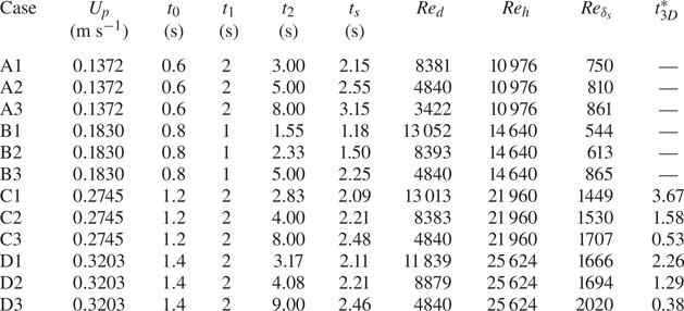
As a measure of the spatial pressure distribution, the variation of the streamwise velocity component in the inviscid region ( $U_x$) along the streamwise direction is shown in figure 2. The velocity profile is shown at half the constant velocity period. Since the acceleration and constant inflow velocity period remain the same, $\alpha$ and $\beta$ remain the same for varying deceleration cases. In figure 2, the continuous line represents the fitted curve, while the symbols represent the velocity obtained from the simulation. The symbols are placed at a distance of 15 grid point spaces between each pair. The velocity variation in the diverging section (from $X = 0.4$ to $X = 1.06$) can be approximated by using the relation
 \begin{equation} U_x = \alpha x^{\beta}, \end{equation}
where  $\alpha$ and $\beta$ are constants and vary with Reynolds number ( $Re_h$). The obtained values for $\alpha$ and $\beta$ for all cases are marked in figure 2.
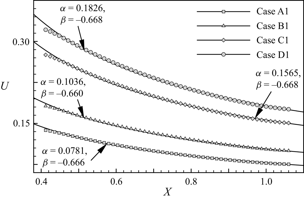
Figure 2. Streamwise velocity variation in inviscid region along the streamwise direction ( $y=1.4286$, $z=1.0$).
The following non-dimensionalized time scales are used to distinguish flow events. At first, flow time is non-dimensionalized by  $t_2$ to differentiate between both the pulse phase and the zero mean inflow period ( $t^* = {t}/{t_2}$). In order to compare different deceleration cases, a non-dimensionalized time scale is identified as $t_d^* = ({t-t_1})/({t_2-t_1})$. Also, a critical flow time associated with three-dimensionally unstable cases, $t^*_{3D}= ({t_{3D} - t_1})/({t_2-t_1})$, is identified from the $t_{3D}$ physical time at which a visible secondary instability initiates in three-dimensionally unstable cases. The $t^*_{3D}$ values observed for cases showing three-dimensional disintegration are provided in table 1. In low and moderate Reynolds number cases, the flow stays in the two-dimensional regime; hence $t^*_{3D}$ is absent for these cases.
2.3. Grid independence and numerical validation
The grid-independent analysis is performed by comparing the evolution of streamwise velocity (case D1) for different grids with elements  $961 \times 193 \times 181$ (grid A), $1501 \times 301 \times 289$ (grid B) and $1921 \times 385 \times 361$ (grid C). Figure 3(a) shows the streamwise velocity through the central axis ( $y=1.3143$, $z=1.0$) of the diverging channel at the end of the constant velocity phase for different grid sizes. The velocity component is non-dimensionalized by the maximum velocity magnitude for the flow instance ( $u^* = {u}/{u_{max}}$). The velocity profiles for three different grid sizes are shown in figure 3(b) following the onset of initial instability at $x = 0.5$, $z = 1.0$. Grids A and B differ by approximately 1.5 %, three times greater than grids B and C. The root-mean-square (r.m.s.) deviation of streamwise velocity component ( $u_{rms}$) of the velocity field during constant mean inflow phase is calculated as
 \begin{equation} u_{rms} = \left( \frac{1}{N} \sum_{l=1}^{l=N} (u'{(l)})^2 \right)^{1/2}, \end{equation}
where the velocity perturbation ( $u'$) is calculated by
 \begin{equation} u'(l) = u(l) - u_{mean}\quad \text{and}\quad u_{mean} = \frac{1}{N} \sum_{l=1}^{l=N} u{(l)}, \end{equation}
for  $N$ snapshots belonging to the constant velocity phase. A comparison of the r.m.s. deviation of the streamwise velocity component developed over the constant mean inflow period reveals a difference of 8.4 % between grids A and B, while the difference between grids B and C is below 4 %. Consequently, grid B is selected for the numerical simulations due to accuracy and computational economy. Based on time step dependency analysis with time steps ranging from $1 \times 10^{-3}$ s to $1 \times 10^{-5}$ s, a time step $1 \times 10^{-4}$ s ( $\textrm {CFL} = 0.02$) was found to be computationally and accurately affordable.
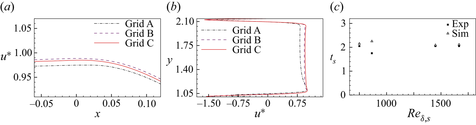
Figure 3. Computational model validation: (a) streamwise velocity variation in the streamwise direction (before separation,  $t^* = 0.631$). (b) Streamwise velocity variation in the wall-normal direction (after separation, $t^* = 0.946$). (c) Experimental comparison of $t_s$.
Comparison of time of flow separation ( $t_s$) with the results of Das et al. (Reference Das, Srinivasan and Arakeri2016) (figure 3b) validates the computational method. The previous experimental works incorporated a two-dimensional simulation of vortex evolution to calculate flow separation time. Here, by taking the flow time and position of zero wall shear stress, we determine the flow separation time and separation point. All the cases show an excellent match with the reported experimental values (less than 8 % difference). An experimental and simulation comparison of the flow field for a high-velocity case is provided in § 3.
3. Initial observations and flow classification
Initially, the contour of non-dimensional spanwise vorticity ( $\omega _z^* = {\omega _z h}/{U_p}$) at various flow instances is used to analyse the evolution at low and high Reynolds number cases. Figure 4 illustrates the contours of spanwise vorticity at six flow instances for low Reynolds number (case A3). The boundary layer thickness increases temporally due to the transient inflow boundary condition (figures 4a,b). The flow generally remains attached to the channel surface during the acceleration and constant velocity phases. Further, the flow undergoes two-dimensional inflectional flow instability during the deceleration phase. Associated vortex formation occurs during either deceleration or the zero mean velocity phases, as reported in previous experiments. The formation of the separation bubble is evident in figure 4(b) at the initial part of the diverging section ( $x = 0- 2$). The initial instability amplifies with the flow time, resulting in shear layer roll-up (figure 4c). Due to the reverse velocity profiles formed near the channel surface during the deceleration phase, the shear layer vortices advect into the upstream region as the flow progresses.

Figure 4. Flow evolution at low Reynolds number case A3: (a) boundary layer thickening, (b) initial oscillation, (c) vortex formation, (d) vortex formation at top wall, (e) vortex detachment, and (f) interaction of top and bottom wall vortices.
Analogous to the bottom wall flow features, the oscillation developed over the top wall moves upstream during the deceleration phase (figure 4d). As a result of the primary negative vortex developed during deceleration, a secondary positive vortex is induced from the bottom wall. During the zero mean inflow phase, vortices eject from the top and bottom channels as a result of the mutual induction of vortex pairs (figure 4e). Further, both top and bottom wall vortices diffuse during the zero inflow phase (figure 4f).
The initial development of flow instability in the case of a high Reynolds number is qualitatively similar to the low Reynolds number case. At high Reynolds numbers, characteristic features such as boundary layer thickening, inflectional instability and shear layer roll-up are observed. However, the subsequent evolution of vortices varies depending on the Reynolds number and deceleration rate. The structures exhibit secondary instability at high Reynolds numbers, and subsequently, the flow becomes turbulent. The spreading and development of three-dimensional structures differ with the deceleration rate.
Figure 5 shows the comparison of flow evolution in numerical simulation with experimental results of Das et al. (Reference Das, Srinivasan and Arakeri2016). At  $t = 3.13$ s, dye visualization manifests the formation of vortices in the diverging part, and similar flow formations are observable in the spanwise vorticity contours of simulation results. Vortex structures spread locally over the initial diverging section ( $x=0.5- 2$). The maximum pressure gradient point also lies in the initial diverging section ( $x\approx 0.46$). The upward movement of vortices is apparent during the deceleration period. Simultaneously coalescence of multiple vortex structures is also noticeable. At $t=5.6$ s, the spanwise vorticity contour of numerical simulation also demonstrates the secondary instability formations. However, only a dense cloud of dye can be seen in the experimental visualization. A three-dimensional development of the vortex interaction makes dye visualization challenging due to the difficulty in identifying individual vortex structures. Localized turbulent vortex formations are observed near the maximum pressure gradient region of the diverging section. Similar to the dye visualization images, the onset of secondary instability over spanwise vortex structures at the end of the constant area section of the channel is visible in the three-dimensional snapshot (figure 5b). The spanwise oscillation evolution is evident, indicating an onset of secondary instability in flow evolution.

Figure 5. Flow evolution at high Reynolds number (case C1) compared with the experimental snapshots of Das et al. (Reference Das, Srinivasan and Arakeri2016): (a) two-dimensional snapshots, and (b) three-dimensional snapshot.
As a result of the APG conditions, inflectional profiles develop, which can eventually lead to boundary layer separation, instability, or both. Figure 6 compares the inflectional nature of flow instability associated with the two-dimensional primary for low and high Reynolds number cases. Figures 6(a) and 6(b) indicate the temporal evolution of instantaneous streamwise velocity profiles developed over the bottom wall in low Reynolds number (case A3) and high Reynolds number (case C1) cases, respectively. During the acceleration phase, the velocity profile is close to the wall surface without any reverse flow region. Here, the velocity profiles are similar to the wall-jet profiles during the deceleration phase. Depending on the Reynolds number and the deceleration rate parameters, reverse flow velocity profiles are observed at specific locations and instances. Since both cases differ in deceleration characteristics, the profiles show slight variations in the initial phase ( $t^*=0.5$).

Figure 6. Velocity profiles across the separation point: (a) bottom wall (case A3,  $x = 0.0615$), (b) bottom wall (case C1, $x = 0.0635$), (c) top wall (case A3), and (d) top wall (case C1).
The flow enters into the deceleration phase resulting in a flow separation in case A3, while case C1 lies in the constant velocity phase. A strong adverse pressure gradient develops when the inflow decelerates, resulting in a reverse flow region. At  $t^* = 0.8$, both cases indicate a reverse flow region, while for case A3, the profile is highly inflectional. In the high-deceleration case C1, the profile is highly inflectional close to the end of deceleration ( $t^* = 0.95$). The extent of the reverse flow zone declines in the zero mean inflow region ( $t^* = 1.15$), and the velocity profiles also alter due to the spanwise vortices passing through the selected point ( $t^* = 1.5$). The velocity profile developed over the top wall is illustrated in figures 6(c) and 6(d) for cases A3 and C1, respectively. Similar to the bottom wall velocity profiles, the top wall velocity profile variations follow the same evolution pattern. Top wall velocity profiles tend to show a higher boundary layer region than bottom wall velocity profiles.
Based on secondary instability features, streamwise vorticity growth and secondary instability initiation time (discussed in detail in subsequent sections), the simulation cases are classified into three categories. A schematic representation of the development of vortices at two critical flow instances in each category is shown in figure 7. The type I category represents low and moderate inflow velocity cases, which do not exhibit spanwise oscillations and remain two-dimensional. Mutual induction of primary and secondary vortices evolved during the flow progression is indicated in the inset on the right of figure 7(a). Vortex pairs stretch, diffuse, and do not exhibit three-dimensional oscillations when in motion.

Figure 7. Illustration of flow evolution for: (a) type I, advecting and decaying two-dimensional vortices; (b) type II, local instability formation; and (c) type III, spatially unstable flow scenarios.
The second category, type II, a secondary vortex that emerges from the bottom boundary in the zero mean inflow phase, exhibits secondary instability and three-dimensional oscillations. Vortex evolution in a locally unstable three-dimensional case (type II) is illustrated in figure 7(b). Here, the value of secondary instability initiation time ( $t^*_{3D}$) is significantly higher than 1. In a rapidly decelerating case, as depicted in the inset on the left of figure 7(b), the flow generally takes a route similar to the two-dimensional instances during the initial stages. Flow structures evolve near the separation bubble and move upstream during the zero mean inflow stage. However, shear layer vortices undergo secondary instability, characterized by a spanwise oscillation with wavelength $\lambda$, as indicated by the second inset in figure 7(b). The spanwise oscillation intensifies with flow time, culminating in a locally turbulent structure.
In the third category, the flow shifts from two-dimensional to three-dimensional during the deceleration phase ( $t^*_{3D} < 1$). The extended deceleration period induces continuous shedding of vortex structures from the separation bubble and advection of the vortex structures. Figure 7(c) illustrates the development of spatially unstable flow with multiple vortices formed over the bottom wall. Due to the streamwise movement of primary vortices over diverging sections, vortex structures downstream merge to form a large structure, further instigating three-dimensional flow characteristics. Advecting three-dimensional structures from the separation bubble and the associated three-dimensional vortices create turbulent flow in the diverging region.
The contour of streamwise vorticity ( $\omega _x = {\partial w}/{\partial Y} - {\partial v}/{\partial Z}$) can reveal the onset and spread of turbulence. A temporally averaged two-dimensional snapshot of non-dimensional streamwise vorticity ( $\omega _x^* = {\omega _x h}/{U_p}$) for three-dimensional cases is presented in figure 8. For $N$ number of snapshots, a temporally averaged streamwise vorticity is obtained by
 \begin{equation} \omega_x^*,{avg} = \frac{1}{N} \sum_{l=1}^{l=N} \omega_x^*{(l)}. \end{equation}
Flow field data between flow instances  $t^*_{st}$ taken as the first snapshot and $t^*_{fi}$ taken as the final snapshot are used to perform temporal averaging, and respective values for each case are given in figure 8. For locally unstable cases (C1, C2, D1 and D2), time step 0.05 s is used, while for spatially unstable cases (C3 and D3), time step 0.1 s is used. The first category of cases (type I) represents two-dimensional spanwise vortices that advect and decay in the channel region. Therefore, a temporal average of streamwise vorticity does not yield valid results for this category (cases A1–A3 and B1–B3) and is hence excluded in figure 8. The second category of cases illustrates the flow features evolving near the separation region. In these cases, the spanwise flow formations remain confined to the entrance of the diverging area and generate three-dimensional oscillations on the secondary vortex structures during the zero mean flow stage. The formation of streamwise vorticity also remains confined to a narrow region near the separation bubble. The third flow category (type III) involves periodic vortex shedding, secondary instability and vortex merging. Flow features develop near the separation region and advect downstream during the deceleration phase. Such cases manifest three-dimensional oscillation in the deceleration phase and disintegrate at a later flow instance. The streamwise vorticity formed over the diverging section is indicative of turbulent advective flow for the third category, as shown in figures 8(e,f). Near the top wall, streamwise vorticity production indicates similar three-dimensional disintegration of top wall vortex structures.
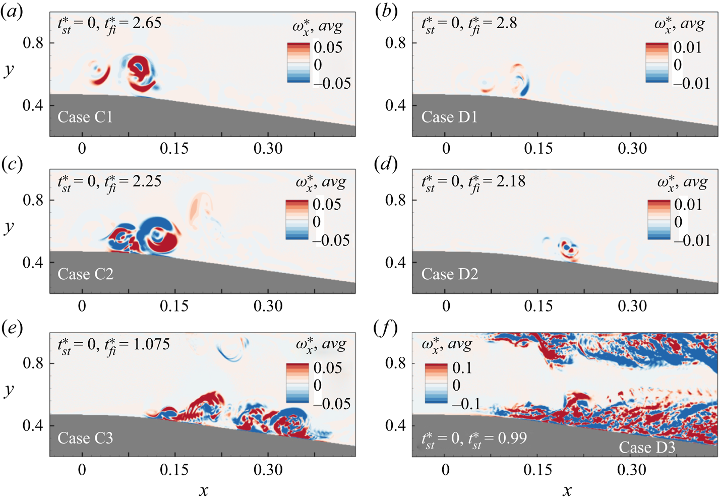
Figure 8. Temporally averaged streamwise vorticity in three-dimensional cases belonging to: (a–d) locally unstable flow evolution cases (type II); and (e,f) spatially unstable flow evolution cases (type III).
The contours of the non-dimensional r.m.s. spanwise velocity component ( $w^*_{rms} = {w_{rms}}/{U_p}$) for all three-dimensional cases are provided in figure 9. The r.m.s. of the spanwise velocity component is calculated using a similar expression of $u_{rms}$ given by (2.10) and (2.11a,b). The evolution of the spanwise component shows a relatively high magnitude near the three-dimensional unstable region, identical to the non-dimensional mean streamwise vorticity (figure 8). The peak fluctuations in the spanwise velocity component spread around the separation bubble for type II cases, indicating a local evolution of the three-dimensional oscillation. Due to the advection of the flow structures during the deceleration period, the intensity of the spanwise fluctuations is higher in spatially unstable cases (type III). In such cases (C3 and D3), advection and later disintegration lead to a spread of the fluctuation intensity over the domain, as shown in figure 9. Identical to the streamwise vorticity contour, spanwise fluctuations are also present over the top wall for type III cases.

Figure 9. R.m.s. of fluctuations in the spanwise velocity component in three-dimensional cases.
4. Type I: advecting and decaying two-dimensional vortices
We now investigate the effect of Reynolds number, and deceleration rate, on vortex flow evolution characteristics in the first flow category. Figure 10 depicts the temporal variation of the Reynolds number based on the displacement thickness calculated using the velocity profile over the separation point for cases belonging to the first category. As the flow accelerates, a thin boundary layer appears over the bottom wall. Broadening of the boundary layer causes an increase in displacement thickness. The displacement thickness remains nearly constant during the constant velocity phase (figure 10). For high-deceleration Reynolds number cases (A1 and B1), deceleration happens in a short period, resulting in a significant increase in displacement thickness. During the zero mean inflow phase, the reverse flow region remains constant, manifesting a constant  $Re_{\delta ^*}$.
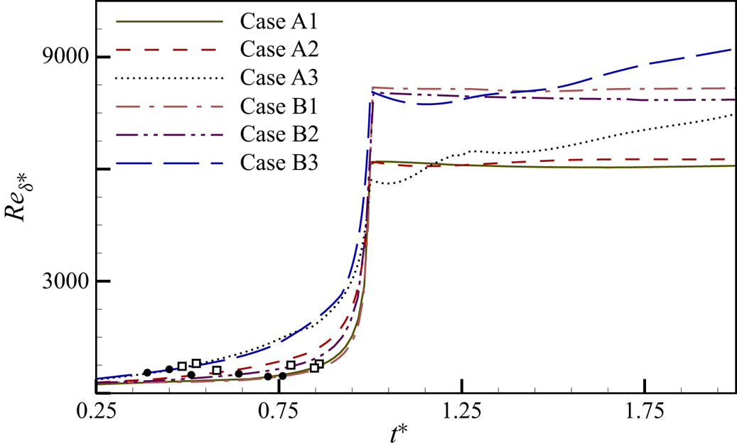
Figure 10. Temporal evolution of Reynolds number based on displacement thickness for advecting and decaying cases (filled circle indicates  $t_s$, open square indicates $t_v$) over the separation point.
Both low and moderate Reynolds number cases show identical flow evolution and are evidenced by the displacement thickness variation. The gradual increase of displacement thickness for low-deceleration cases (A3 and B3) is attributed to the more extended deceleration period. The time at which wall shear stress is zero ( $t_s$) and vortex formation time ( $t_v$) are marked with filled circle and hollow square symbols, respectively. Figure 10 shows that two-dimensional flow separations occur in the $Re_{\delta ^*}$ band 420–640, and vortex formation occurs between 560 and 780. During the zero mean inflow phase, the vortices pass across the separation point, causing the abnormality in the temporal variation of displacement Reynolds number.
The three-dimensional vortex structures developed in the zero mean inflow phase ( $t^* = 2.0$) for advecting and decaying cases exhibit distinct two-dimensional evolution characteristics (figure 11). The initial flow develops along the general route of broadening boundary layer thickness and inflectional streamwise velocity profile, followed by flow separation. In figure 11, the most amplified vortex pair formed due to the inflectional instability is labelled $BV$ and $bv$ for primary and secondary vortices, respectively. Vortex structures advect upstream due to the reverse velocity in the boundary layer during the zero mean inflow phase. In high and moderate-deceleration cases (A1 and A2), the vortex structures remain close to the bottom wall boundary (figures 11a,b). The induced angular velocity by the vortex pair is shown to be more substantial for moderate deceleration (case A2) compared to the high-deceleration case (A1), pushing the vortex pair towards the top wall. The flow evolution in the low-deceleration case (A3) shows multiple vortex formations in the diverging and constant channel regions. The extended deceleration period leads to the development of multiple vortices, advecting upstream in later flow instances.

Figure 11. Spanwise vortex roll-up in two-dimensional (type I) flow evolution cases: (a) case A1, (b) case A2, (c) case A3, (d) case B1, (e) case B2, and (f) case B3.
Flow evolution in the moderate Reynolds number cases (B1, B2 and B3) is qualitatively similar to the low Reynolds number case. Compared to low Reynolds number cases, the flow structures in moderate Reynolds number cases lie in the initial stages. Figures 11(d) and 11(e) reveal the presence of a noticeable vortex pair at  $x = 0$, which is comparable to the respective deceleration cases in the low flow Reynolds number regime. The vortex structures are well developed in the low-deceleration case (B3), similar to case A3. As shown in figure 11(f), vorticity rolls form in the diverging and constant channel regions. In case B3, the streamwise location of the magnified vortex structure lies in the diverging section ( $x = 1- 2$), as in case A3. The vorticity patch in figure 11(f) indicates that the vortex is beginning to form over the top wall, signifying a higher vortex formation on both the top and bottom walls during the dead inflow phase.
The advective nature of the vortices and their influence on the deceleration rate are quantified by tracking the vortex core trajectory. The core of the vortex is identified by minimum and maximum vorticity for primary ( $BV$) and secondary ( $bv$) vortices, respectively. Figure 12 shows the temporal evolution vortex core for the primary negative vortex and the secondary positive vortex for cases A1, A2 and A3. The time step between the data points for negative and positive vortices is distinct within each case, which is marked aside from the core positions in figure 12. In high-deceleration events (case A1), the flow evolution happens near the end of the constant channel region ( $x = -0.4- 0$), as shown in figure 12(a). Prior to being ejected into the core flow area, primary and secondary vortices developed over the bottom wall advect upstream. Increasing the deceleration period causes the vortices to develop during the deceleration phase in the downstream region. The vortex core position in figure 12(b) shows the advection of developed vortices upstream during the early part of the zero mean inflow period in case A2. Vortex cores moving upwards are apparent in the low-deceleration case (figure 12c). Contrary to the high-deceleration case, the vortex pair moves closer to the top wall and interacts with the top wall vortices in the low-deceleration case.

Figure 12. Temporal evolution of vortex core in advecting cases: (a) case A1 (first data point  $t^* = 1.33$, last data point $t^* = 3.833$); (b) case A2 ( $t^*$ from 1.15 to 2.4); and (c) case A3 ( $t^*$ from 1.375 to 2.8).
To quantify vorticity generation, the temporal evolution of the circulation-based Reynolds number is presented in figure 13(a). The circulation within the channel region is calculated by considering a subdomain, as shown in figure 1(b). This small domain can characterize both positive and negative vortex formations near the bottom wall, while skipping the boundary layer vorticities and avoiding interference from the top wall structures. The stronger vortex flow features developed in the low-deceleration cases (A3 and B3) cause an increase in circulation during the deceleration period. For high-deceleration cases (A1 and B1), spanwise vortex roll-up is weaker compared to the low-deceleration cases, resulting in a flatter circulation Reynolds number curve. As the flow stage proceeds into zero mean inflow, the primary vortex interaction over the channel surface leads to the production of positive vortices. The generation of a positive vortex roll-up and subsequent diffusion decay contribute to a decline in circulation during the zero mean inflow phase.

Figure 13. Temporal evolution of (a) spanwise Reynolds number based on circulation, and (b) maximum spanwise vorticity, for advecting and decaying cases (filled circle indicates  $t_s$, open square indicates $t_v$).
A quantitative analysis of the temporal evolution maximum spanwise vorticity magnitude of the primary vortex ( $BV$) against non-dimensionalized deceleration time is provided in figure 13(b). Vortex formation begins towards the end of the deceleration phase in cases A1 and B1. During the zero mean inflow period, the primary vortex in cases A1 and B1 reaches its maximum vorticity in a short time, as shown in figure 13(b). In low- and moderate-deceleration cases, flow separation is achieved during the deceleration period, and the vorticity magnitude attains its maximum at the end of the deceleration phase. Unlike the high-deceleration cases, low-deceleration cases attain maximum vorticity magnitude during the initial deceleration phase. All cases show a steady reduction of the vorticity magnitude with an identical slope indicating the decay of vortex flow structures.
5. Type II: locally evolving three-dimensional vortices
The growth of the boundary layer prior to inflectional instability is qualitatively the same in type II cases as in type I. The temporal evolution of the displacement thickness based on Reynolds number for high Reynolds number cases is depicted in figure 14(a). The displacement thickness increases when the boundary layer broadens due to deceleration. These cases exhibit flow separation in a  $Re_{\delta ^*}$ range 840–1050, while vortex formation occurs in a higher range of $Re_{\delta ^*}$ (970–1170). It is evident that displacement thickness for very high Reynolds number cases (D1 and D2) is much higher at the end of the deceleration phase than for high Reynolds number cases (C1 and C2). The generation of vortices during the zero mean inflow period leads to an erratic variation in displacement thickness. Similar to type I cases, the circulation evolution in high Reynolds number cases reaches a maximum and subsequently drops. Cases C1 and D1 with high deceleration demonstrate a sustained rise in circulation even after the deceleration phase, implying vortex development in the zero mean inflow period. Vortex generation near the end of the deceleration period results in maximum circulation in moderate-deceleration cases (C2 and D2).

Figure 14. Temporal evolution of (a) Reynolds number based on displacement thickness, and (b) Reynolds number based on spanwise circulation, for locally unstable cases (filled circle indicates  $t_s$, open square indicates $t_v$).
The evolution of fluctuations in the spanwise velocity component can characterize the growth of the three-dimensional flow disturbances in the flow domain. In the present simulation, the source of perturbations is limited to the two-dimensional fluctuations associated with the analytical solution, which are imposed at the inlet of the domain, and the unavoidable numerical error related to the numerical scheme. As shown in the simulation, these values are of the order of  $10^{-6}$. In figure 15, the evolution of the amplitude of the spanwise fluctuations ( $(w')^2 = {(w-w_{mean})^2}/{U_p^2}$) is plotted for locally three-dimensional cases. The probe location is selected as the maximum spanwise velocity component average position.

Figure 15. Growth of the spanwise velocity component fluctuation in type II cases.
For all cases, the non-dimensional spanwise fluctuation amplitude increases during the dead inflow region, indicating the three-dimensional disintegration process. Oscillation amplitudes reach high magnitudes for very high Reynolds cases (D1 and D2) and are near 0.01, whereas they peak at around 0.005 for high Reynolds cases. Also, the spanwise velocity component growth is affected by the deceleration period. While low-deceleration cases (C1 and D1) achieve their peak amplitudes later, after the pulse ends, moderate-deceleration cases (C2 and D2) attain their peak amplitudes earlier. The highest amplitude is observed in case D2, with a sharp increase in the oscillation amplitude.
5.1. The emergence of secondary instability and local breakdown
In high Reynolds numbers, the vortices formed by two-dimensional primary inflectional instability further undergo secondary instability, creating three-dimensional structures. Vortex flow structures developing in a high-deceleration case (C1) are revealed by the iso-surfaces of non-dimensionalized spanwise vorticity in figure 16. Primary inflectional instability causes the formation of negative vortices (LP1–LP4), which further induces secondary positive vortices (lp1–lp4) from the bottom wall boundary layer (figure 16a). This secondary vortex and the primary vortex form a pair near the wall proximity. Due to the mutual induction of the vortices, the pair detaches from the bottom wall, still pertaining to the two-dimensional nature ( $t^* = 1.25$). Most flow features evolve near the initial diverging section emphasized by the non-dimensionalized streamwise scale on the top wall. The induced angular velocity of the upstream vortex pair (LP1, lp1) drives them to roll towards the vortex pair at the downstream location, (LP2, lp2). Such a flow development results in stretching and splitting of the positive secondary vortex by the primary vortices (lp2a, lp2b in figure 16b). The residual momentum pushes the secondary vortex (lp1) from the upstream pair to join the downstream couple; such a tri-vortex group further amplifies the roll-on process ( $t^* = 1.93$). Inflectional profiles in the boundary layer seed multiple vortices from the boundary layer, as portrayed in figure 16(b) (pairs 5 and 6).

Figure 16. Temporal evolution of three-dimensional flow features identified by spanwise vorticity for case C1.
The secondary vortex structure (lp2b) exhibits a spanwise oscillation while orbiting the primary vortex (LP1), as shown in figure 16(c). Similar vortex flow features are exhibited by the vortex pairs detaching from the bottom wall surfaces downstream (pairs 3 and 4). A secondary vortex (lp4) downstream ( $x\approx 1.0$) undergoes a similar fashion of vortex splitting, creating multiple positive vortices as in the former time instances for the upstream secondary vortex (lp2).
The merging of the primary vortex cores (LP4 and LP6) is visible in the same instance ( $t^* = 1.93$). As the flow progresses, oscillations amplify in the secondary vortex circling the primary vortex. A sandwiching effect of the merged negative vortex cores (MG1 and MG2) stretches the secondary vortices around them (figure 16d). After the stretching, spanwise oscillations disintegrate into loops around the primary spanwise vortex flow structures (MG1 and MG2). However, the initially ejected secondary vortex (lp1) survives the vortex interactions and shows a three-dimensional oscillation while orbiting the primary vortex. In a later flow instance ( $t^* = 2.72$), the secondary vortex structure breaks down into spanwise loops around partially disintegrating primary vortices (LP1; figure 16e). A complete transition to a turbulent structure with a negative vorticity core is observed as the flow progresses ( $t^* = 3.18$). Simultaneous production of two-dimensional vortices and merging transitions is observable in the upstream and downstream positions in figure 16(f). Since this flow development lies in the zero mean inflow phase, advection of three-dimensional roll-ups is not evidenced for case C1, and flow features are confined to a small area near the initial diverging section ( $x = 0.4- 1.5$). For case C1, flow evolution over the top wall has not yet been developed at $t^* = 3.18$. Induction from the bottom wall vortices creates a positive vorticity patch over the top wall at $t^* = 3.18$, indicating vortex roll-up in later flow time.
The three-dimensional topology of vortex structures is identified further using the  $\lambda _2$ method and contoured by non-dimensional streamwise vorticity in figure 17, which illustrates the spanwise oscillation developed over the secondary vortex for case C1 at $t^* = 1.93$. The alternate streamwise vorticity originated over the spanwise vortex roll-ups displays a symmetrical pattern. A cross-section ( $Y$–
$Y$– $Z$) through the central plane of vortex pairs ( $x = 0.308$) is taken, to understand the nature of oscillations. Non-dimensionalized spanwise vorticity contoured snapshots (figure 17b) provide a clear visual of secondary vortex developing oscillations. The presence of alternating streamwise vorticity is further explained by superimposing the vector plot in figure 17(c). Circulation regions are discernible over the spanwise vortex roll-ups, as seen in the inset.

Figure 17. (a) Flow features identified (LP1 and lp2b) using the  $\lambda _2$ method contoured by streamwise vorticity ( $\lambda _2 = -1$). (b) Section through the spanwise oscillation contoured by spanwise vorticity ( $x = 0.29$). (c) Section through the spanwise oscillation contoured by streamwise vorticity.
The temporal evolution of flow vortices in cases similar to case C1 (type II) is evidenced in figure 18. Vortex flow structures at two flow instances are shown: the first flow instance portrays the three-dimensional oscillations during the early transition phase, while the second instance illustrates the flow structures in the turbulent phase. Identical to case C1, primary instability in the deceleration phase develops into a vortex pair, which moves downstream and interacts with similar vortex pairs. Figures 18(a,b) indicate the formation of spanwise oscillations over the secondary vortices in case C2. Stretching of the secondary vortex around the primary vortex is evidenced at  $t^* = 2.0$. Along with three-dimensional disintegration, vortex pairs eject into the flow core at a downstream position due to the induced velocity. As flow progresses, analogous to case C1, the formation of a turbulent three-dimensional structure with negative spanwise vorticity is illustrated in figures 18(a,b). Unlike case C1, the formation of top wall vortices is evidenced for case C2 as depicted in figures 18(a,b). During the zero mean inflow phase at $t^* = 2.13$, the ejected vortex pair interacts with the top wall boundary layer. Figures 18(c,d) and 18(e,f) show identical flow evolution for cases D1 and D2. Three-dimensional disintegration initiates with vortex pair interaction, resulting in a locally turbulent region. The turbulent region develops earlier for high Reynolds number cases (D1 and D2) than for high flow Reynolds number cases (C1 and C2).

Figure 18. Temporal evolution of three-dimensional flow features identified by spanwise vorticity for cases belonging to type II instability: (a,b) case C2, (c,d) case D1, and (e,f) case D2.
5.2. Modelling of secondary instability
The DMD algorithm is used to analyse secondary instability over the shear layer vortices resulting from primary inflectional instability; it identifies the underlying dynamics of the coherent flow features developed during the flow evolution. We use the snapshot-based approach introduced by Schmid (Reference Schmid2010) to identify the secondary instability features along with their temporal dynamics. A review by Taira et al. (Reference Taira, Hemati, Brunton, Sun, Duraisamy, Bagheri, Dawson and Yeh2020) offers further examples of this approach to identify underlying features in many transitional and turbulent flows.
The DMD algorithm starts by arranging state vectors from simulation data snapshots column-wise into two snapshot matrices  $\boldsymbol {U}_1$ and $\boldsymbol {U}_2$, with two consecutive time intervals ( $\Delta \tau$). DMD analysis identifies a best-fit linear operator $\boldsymbol {A}$ that relates matrix $\boldsymbol {U}_1$ to the matrix $\boldsymbol {U}_2$:
 \begin{equation} \boldsymbol{U}_2 = \boldsymbol{A} \boldsymbol{U}_1. \end{equation}
By taking the singular value decomposition (SVD) of the snapshot matrix ( $\boldsymbol {U}_1$), we obtain left and right eigenvectors ( $\boldsymbol {S}$ and $\boldsymbol {D}$, respectively), along with the eigenvalue ( $\varLambda$). In order to build a best-fit linear operator correlating both matrices, we take the pseudo-inverse of $\boldsymbol {U}_1$ (by taking the conjugate transposes of SVD vectors ( $\boldsymbol {S}^*,\boldsymbol {D}^*$) together with $\boldsymbol {U}_2$ as follows:
 \begin{equation} \boldsymbol{\mathsf{A}} = \boldsymbol{U}_2 \boldsymbol{D}^* \varLambda^{-1} \boldsymbol{S}^*. \end{equation}
 By eigen-decomposition, the low-dimensional model is decomposed into eigenvector ( $\boldsymbol {W}$) and eigenvalues ( $\boldsymbol {\lambda }_D$). The temporal dynamics of the system can be identified from the eigenvalues using the following relations for growth rate and frequency:
 $$\begin{gather} \sigma_{DMD} = \frac{\log\left({\rm Re}(\lambda_D)\right)}{2 {\rm \pi}\, \Delta \tau}, \end{gather}$$
 $$\begin{gather}f_{DMD} = \frac{\log\left({\rm Im}(\lambda_D)\right)}{2 {\rm \pi}\,\Delta \tau}. \end{gather}$$
 In order to obtain the DMD modes ( $\varPhi$), the low-dimensional model is reconstructed from its eigenvectors as
 \begin{equation} \boldsymbol{\varPhi} = \boldsymbol{U}_2 \boldsymbol{D}\varLambda^{-1}\boldsymbol{W}. \end{equation}
 Through a three-dimensional DMD of streamwise vorticity data, the most unstable flow features associated with secondary instabilities are identified (figure 19). For the DMD calculation, three-dimensional snapshots are taken with time step  $\Delta \tau =0.05$ s between each snapshot. The Ritz circle obtained from the DMD for cases belonging to the second category is presented in figure 19(a). The position of the mode with respect to the unit circle outlined in the figure indicates the stability of the modes. In general, a mode lying outside a circle indicates an unstable mode, while lying within signifies a stable mode; and when it lies on a circle, it is neutrally stable. In all cases, at least one mode displays an unstable trait, illustrated by the circle in figure 19(a). Figure 19(b) shows the growth rate and frequency distribution for the DMD modes. The highest growth rate mode obtained from DMD analysis is indicated by $1_{\sigma }$.

Figure 19. Three-dimensional DMD analysis results: (a) Ritz circle, (b) growth rate versus frequency, and (c) leading secondary instability modes based on growth rate criterion for type II cases.
When streamwise vortex growth is unstable, vortex roll-ups will experience three-dimensional destabilization, as manifested by the positive growth rates for all cases. Unstable three-dimensional modes are identified through the growth rate criteria for all cases and are shown in figure 19. The three-dimensional morphology of unstable modes is visualized using an iso-surface of streamwise vorticity. A spanwise variation of the streamwise vorticity is evidenced in all cases. The spanwise wavelength obtained for the mode with the highest growth rate is provided in table 2. Averaging the distance between the peaks of the streamwise vorticity plotted across the vortex core provides the mean spanwise wavelength. The average spanwise wavelength observed for all three-dimensional cases is tabulated in table 2. Both wavelengths are non-dimensionalized by the distance between the cores of vortex pairs ( $b$ is the distance between maximum and minimum vorticity magnitudes). The spanwise wavelength for the coherent flow features identified by DMD analysis ( $\lambda _{DMD}$) lies close to the mean spanwise wavelength determined from streamwise vorticity variation over the oscillation ( $\lambda _{mean}$).
Table 2. Spanwise wavelength comparison and parameters for Lamb–Oseen approximation.
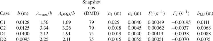
The secondary instabilities are formed during the zero mean phase in cases belonging to the type II category, which is similar to the short-wavelength elliptic instability demonstrated by Laporte & Corjon (Reference Laporte and Corjon2000). Since multiple vortex pairs are observed near the bottom wall, unlike classical short wavelength vortex instability, theoretical stability analysis is performed for most magnified vortex pairs. Variation of the spanwise vorticity in a vortex pair ejecting from the bottom wall (case C1) is shown in figure 20(a). An identical depiction of an approximated Lamb–Oseen pair obtained from (5.6) is given in figure 20(b). The vorticity distribution for such a vortex pair with circulations  $\varGamma _1$ and $\varGamma _2$ may be approximated using the Lamb–Oseen equation (Leweke et al. Reference Leweke, Le Dizes and Williamson2016)
 \begin{equation} \omega_z = \frac{\varGamma_1}{{\rm \pi} a_1^2}\exp\left(-\frac{r^2}{a_1^2}\right) + \frac{\varGamma_2}{{\rm \pi} a_2^2}\exp\left(-\frac{r^2}{a_2^2}\right), \end{equation}
where  $r$ represents the distance from the vortex core position. The core radius ( $a_1$ and $a_2$) for a vortex centred at $\boldsymbol {X}^c$ is obtained from
 $$\begin{gather} (x_{c_1},y_{c_1}) = \left(\frac{1}{\varGamma_1}\int_{D_1} x \omega_z\, {\rm d}S, \ \frac{1}{\varGamma_1}\int_{D_1} y \omega_z\,{\rm d}S\right), \end{gather}$$
 $$\begin{gather}a_1^2 = \frac{1}{\varGamma}\int_{D_1}|\boldsymbol{X}-\boldsymbol{X}^c|^2 \omega_z \,{\rm d}S, \end{gather}$$
where  $D_1$ represents the domain containing each vortex, $\omega _z$ defines the spanwise vorticity, and $\textrm {d}S$ represents the infinitesimal area.

Figure 20. Depiction of Lamb–Oseen model: (a) simulation, (b) Lamb–Oseen model, and (c) Lamb–Oseen model comparison for vortex pair in locally unstable cases.
To ascertain the validity of the Lamb–Oseen approximation, the plot of the spanwise vorticity obtained from (5.6) is compared with the simulation results (through the vorticity cores). Table 2 provides the essential parameters obtained from simulation used to estimate the Lamb–Oseen approximation for locally unstable cases (type II) as depicted in figure 20(c). Here,  $b_{LO}$ denotes the distance between the first positive vortex core and the second negative vortex in approximated vorticity distribution. In cases C1, C2 and D2, a vertical pair of vortices is compared with a vertical Lamb–Oseen pair, while in case D1, a better approximation is obtained for a horizontal pair and is compared to a similar Lamb–Oseen approximation (figure 20c). As presented in figure 20, the assumption of a Lamb–Oseen vortex approximation remains true in all selected flow instances.
Le Dizes & Laporte (Reference Le Dizes and Laporte2002) proposed an explicit relation using approximate linear expressions for the internal strain ratio ( $s_r$) and inertial wave vector inclination for predicting the growth rate of an elliptic instability in a counter-rotating vortex pair. Leweke et al. (Reference Leweke, Le Dizes and Williamson2016), in their review, presented a revised linear fit to determine the frequencies ( $\omega$) and damping rates ( $\zeta$) of the first two Kelvin modes. The growth rate for the first two modes of elliptic instability in a Lamb–Oseen vortex pair is given by
 \begin{align} \sigma_1^{*,{(n)}} = \sqrt{\left(\frac{3}{4} - \frac{\bar{\varOmega}_1}{4}\right)^4 s_r^2\left(\bar{\varOmega}_1\right)\left(\frac{\varGamma_2}{\varGamma_1}\right)^2 - \left(\omega^{(n)}- \bar{\varOmega}_1\right)^2 \left(\frac{b}{a_1}\right)^4}- \left(\frac{b}{ a_1}\right)^2 \left(\frac{\zeta^{(n)}}{Re_{\varGamma_1}}\right) . \end{align}
The superscript  $n$ represents the mode number, and the subscript denotes the vortex number. Here, the growth rate of the mode is non-dimensionalized by the time scale of translational motion ( ${2{\rm \pi} b^2}/{\varGamma _1}$). Linear expressions for real ( $\omega$) and imaginary ( $\zeta$) parts of the complex frequency in (5.9) are
 $$\begin{gather} \bar{\varOmega}_1 = \left(\frac{a_1}{b}\right)^2\left(\frac{\varGamma_1 + \varGamma_2}{\varGamma_1}\right) , \end{gather}$$
 $$\begin{gather}s_r(\bar{\varOmega}) = 1.5+0.1323\left(0.32-\bar{\varOmega}\right)^{-9/5} , \end{gather}$$
 $$\begin{gather}\omega^{(1)} =-0.135\left(ka_1 - 2.26\right), \end{gather}$$
 $$\begin{gather}\omega^{(2)} =-0.084\left(ka_1 - 3.95\right), \end{gather}$$
 $$\begin{gather}\zeta^{(1)} = 74.02 + 64.15\left(ka_1 - 2.26\right) , \end{gather}$$
 $$\begin{gather}\zeta^{(2)} = 229.6 + 104.3\left(ka_1 - 3.95\right) . \end{gather}$$
Using (5.9), the growth rate of elliptical instability for a counter-rotating vortex pair ejected from the bottom boundary of the wall was determined. The growth rate curves obtained for different spanwise wavenumbers for secondary vortices are presented in figure 21. A similar analysis was conducted on the vortex structures in type I cases. The secondary vortices, which develop in two-dimensional advecting and diffusing cases, indicate stable growth rates and have been confirmed by our calculations but are not shown. The growth rate curves are calculated for the secondary vortex, which undergoes three-dimensional disintegration (using Lamb–Oseen approximation as shown in figure 20c). The growth rate curves indicate an unstable first mode alongside a stable second mode (figure 21a). An identical growth rate curve is obtained for case D1 (figure 21b), revealing the formation of first-mode elliptic instability in high-deceleration cases (C1 and D1). Unlike high-deceleration cases, both the first and second modes show an unstable nature in moderate-deceleration cases (C2 and D2) (figures 21c,d).

Figure 21. Growth rate curves for first and second elliptic modes for secondary vortex in locally unstable cases: (a) case C1, (b) case D1, (c) case C2, and (d) case D2.
The temporal growth of vorticity/spanwise oscillation can be associated with the secondary instability (elliptic instability) of the shear layer vortices formed by the primary instability mechanism. The small spanwise velocity component can grow into a larger magnitude if the flow conditions are susceptible to elliptical instability. The fluctuations amplify due to the elliptic instability to a significant value ( $10^{-2}$) for all type II cases, as is evident in figure 15, whereas it is negligible for type I cases. We also found that the amplitude of spanwise fluctuation is higher for case D2, showing a maximum growth rate. Identical to the growth rate curves, case D2 indicates a maximum amplitude of order 0.01. Compared to very high Reynolds cases (D1 and D2), high Reynolds cases (C1 and C2) possess lower amplitude, and the growth rate for case C1 shows the lowest value.
6. Type III: spatially unstable flow evolution
Three-dimensional disintegration of vortex flow features results in complex boundary layer growth in spatially unstable cases (figure 22a). In both cases,  $Re_{\delta ^*}$ evolution initiates with a low value during the acceleration phase. The flow separation for cases C3 and D3 lies at $Re_{\delta ^*}=980$ and $1133$, respectively, which is the highest compared to the former categories. Similarly, vortex formation initiates in case C3 at $Re_{\delta ^*} = 1092$, whereas in case D3 it is at $Re_{\delta ^*} = 1300$. Unlike in other cases, flow generates vortex roll-up during the initial deceleration stage, reflected by an increase in displacement thickness. As the vortex clears, the profile returns to its typical profile, lowering the displacement thickness. The peaks of the displacement thickness variation indicate further vortex development. The three-dimensional vortex breakdown in both cases produces high-frequency oscillations during the flow advancement. Three-dimensional disintegration initiates more quickly for case D3 (around $t^* = 0.7$) due to the higher streamwise velocity, compared to case C3. Alternatively, case C3 displays three-dimensional turbulent behaviour towards the end of the deceleration phase (around $t^* = 0.9$).

Figure 22. Temporal evolution of (a) Reynolds number based on displacement thickness, and (b) Reynolds number based on spanwise circulation, for spatially unstable cases (filled circle indicates  $t_s$, open square indicates $t_v$).
Oscillations in the temporal variation of the Reynolds number based on spanwise circulation indicate a transition from a two-dimensional to a three-dimensional flow regime (figure 22b). Cases C3 and D3 display an increment in circulation during the acceleration and constant velocity phases, identical to cases A3 and B3. Compared to the previous categories, during the deceleration phase, the circulation-based Reynolds number reaches a higher magnitude for these cases (C3 and D3), indicating higher vortex formation. Minute spanwise loop formation due to three-dimensional disintegration induces oscillations in circulation development during the deceleration phase. The earlier onset of fluctuations characterizes the rapid disintegration of flow structures in case D3 compared to case C3. The circulation decays during the zero mean inflow phase with a higher decay rate compared to type I cases.
6.1. Unsteady separation and flow breakdown
Vortex flow structures identified by the non-dimensional spanwise vorticity in case C3 are portrayed in figure 23. Shear layer roll-ups marked by BS1–BS5 are observed at nearly equally spaced locations over the diverging section. Vortex flow structures are highlighted according to their formation sequence during flow evolution. Due to unsteady flow separation, vortices develop over the initial diverging section (PS1) during deceleration. Vortices evolving over the diverging section advect downstream, creating additional positive vortices (bs1) from the wall surface ( $t^* = 0.55$). Persistent streamwise velocity deceleration leads to a continuous shedding of vortices from the initial diverging section (PS1 and PS2). A higher advective velocity of the upstream vortex leads to the pairing of the vortex roll-ups (BS1 and BS3, $t^* = 0.63$). Due to mutual induction, positive vortices (ps1a–ps1c) eject from the bottom wall vorticity layer and revolve around the primary vortex (PS1) while advecting downstream ( $t^* = 0.69$). In such advecting vortex pairs, secondary vortices generate spanwise oscillations (ps1c) similar to locally unstable cases (type II). The formation of three-dimensional oscillations is attributed to the local interaction of advecting pairs. Simultaneous merging of vortex flow features (BS2 and BS4) and the three-dimensional disintegration of secondary vortices (ps1c, ps2a and ps2b) are evident in later deceleration flow instances ( $t^* = 0.74$ and $0.76$).

Figure 23. Temporal evolution of three-dimensional flow features identified by non-dimensional spanwise vorticity for case C3.
A complex structure with multiple small-scale vortices is formed due to the growth of the three-dimensional oscillations into tube-like structures (MG4), which displace downstream due to the streamwise velocity ( $t^* = 0.81$). Three-dimensional oscillations develop over the unsteady separation vortices when the flow passes half of the deceleration phase. A vortex pair discharging from the initial diverging section displays three-dimensional oscillation after the ejection ( $t^* = 0.91$). Advecting vortex roll-ups interact with other flow features, generating a turbulent flow structure ( $t^* = 0.91$). The decay of streamwise velocity further results in flow detachment, leading to a turbulent flow evolution during the zero mean inflow phase. Analogous to the former category, the flow features move backwards as the flow progresses in the zero mean inflow region. Tiny loop structures are formed through the disintegration of vortex flow structures at later flow instances ( $t^* = 1.18$).
Identical to the bottom wall, the top wall boundary layer displays vortex roll-ups and three-dimensional disintegration, as presented in figure 23. An extended stay of the bottom wall vortex in the initial diverging section induces the flow to separate from the top wall leading to vortex roll-up. The top wall boundary layer broadens over the bottom separation region once the flow separates over the bottom wall ( $t^* = 0.55$). In type III cases, flow separation occurs earlier in the deceleration phase, forcing the fluid over the top wall. Formation of a primary positive top wall vortex (TS1) subsequently results in the production of a negative secondary vortex (ts1, $t^* = 0.69$). The shedding of vortices due to unsteady separation promotes the development of flow structures (TS pairs 2 and 3) across the top wall ( $t^* = 0.74$). The top wall vortices retain their two-dimensional traits, while the bottom wall vortex pair undergoes three-dimensional disintegration at $t^* = 0.76$. Due to induced rotation, primary and secondary top wall vortices eject from the top wall boundary layer ( $t^* = 0.81$). Analogous to the bottom wall flow features, top wall vortices clearly show the pairing behaviour at $t^* = 0.91$ (TS3). Towards the end of the deceleration phase, the top wall formations also generate three-dimensional oscillations. In the initial zero mean inflow phase, the interaction between the top and bottom wall structures is minimal ( $t^* = 1.02$), while at a later flow instance ( $t^* = 1.18$), the mixing of flow features over the top and bottom walls results in a turbulent flow evolution.
Similar to case C3, vortex evolution in case D3 demonstrates vortex generation and three-dimensional breakdown of flow characteristics during the deceleration phase (figure 24). The inflectional instability in the boundary layer develops into vortex roll-ups (BS1–BS5) during the deceleration phase ( $t^* = 0.43$ and $0.49$). Compared to case C3, a higher mean inflow velocity results in a higher advective velocity for the flow features along with the vortex shedding (PS pairs) due to unsteady separation ( $t^* = 0.52$). Three-dimensional oscillations induced over the secondary vortices amplify and disintegrate at subsequent flow instances as vortex pairs are ejected from the initial diverging section. In case D3, the vortex flow patterns disintegrate at an early pulse stage, resulting in an advecting turbulent structure that stays closer to the bottom wall ( $t^* = 0.6, 0.64$). Unlike case C3, the top wall vortices (TS pairs 1 and 2) advect downstream along with the bottom wall structures due to the earlier inception of top wall structures. Flow formations over the top wall retain their two-dimensional nature at this flow instance ( $t^* = 0.64$). As the flow moves forward through the deceleration phase, the advecting top wall vortices (TS1, TS2) evidence three-dimensional disintegration ( $t^* = 0.7$). The turbulent flow features over the top and bottom walls advect downstream as flow forwards, while the interaction of the structures results in a turbulent flow as evidenced at $t^* = 0.75$ and $0.82$.

Figure 24. Temporal evolution of three-dimensional flow features identified by non-dimensional spanwise vorticity for case D3.
A separation bubble forms near the initial diverging region due to unsteady separation, constituting a spanwise vortex roll and induced positive vortex in the boundary layer. A close-up image of the vortex shedding and three-dimensional disintegration of the separation bubble vortices is illustrated in figure 25. Similar to the shedding process observed by Wissink & Rodi (Reference Wissink and Rodi2006), consecutive formation of the vortex rolls is evidenced during the deceleration phase (figure 24). As the flow decelerates further, the streamwise velocity weakens, amplifying the perturbations developing due to vortex interactions. As the flow decelerates ( $t^* = 0.61$), the secondary vortices generate a spanwise oscillation during the shedding process, and develop into spanwise loops over the primary negative vortex (PS2). Decay in streamwise velocity induces an oscillation in the separation bubble due to the amplification of perturbations (PS3). As the flow progress ( $t^* = 0.63$), the vortex structure (PS3) sheds downstream, creating a short interval and a turbulent separation bubble (PS4). Further deceleration leads to the disintegration of the separation bubble and moves to a turbulent regime ( $t^* = 0.65$). The formation of a turbulent separation bubble leads to an uneven shedding of the turbulent flow features similar to the flow evolution observed by Wissink & Rodi (Reference Wissink and Rodi2006) ( $t^* = 0.68$).
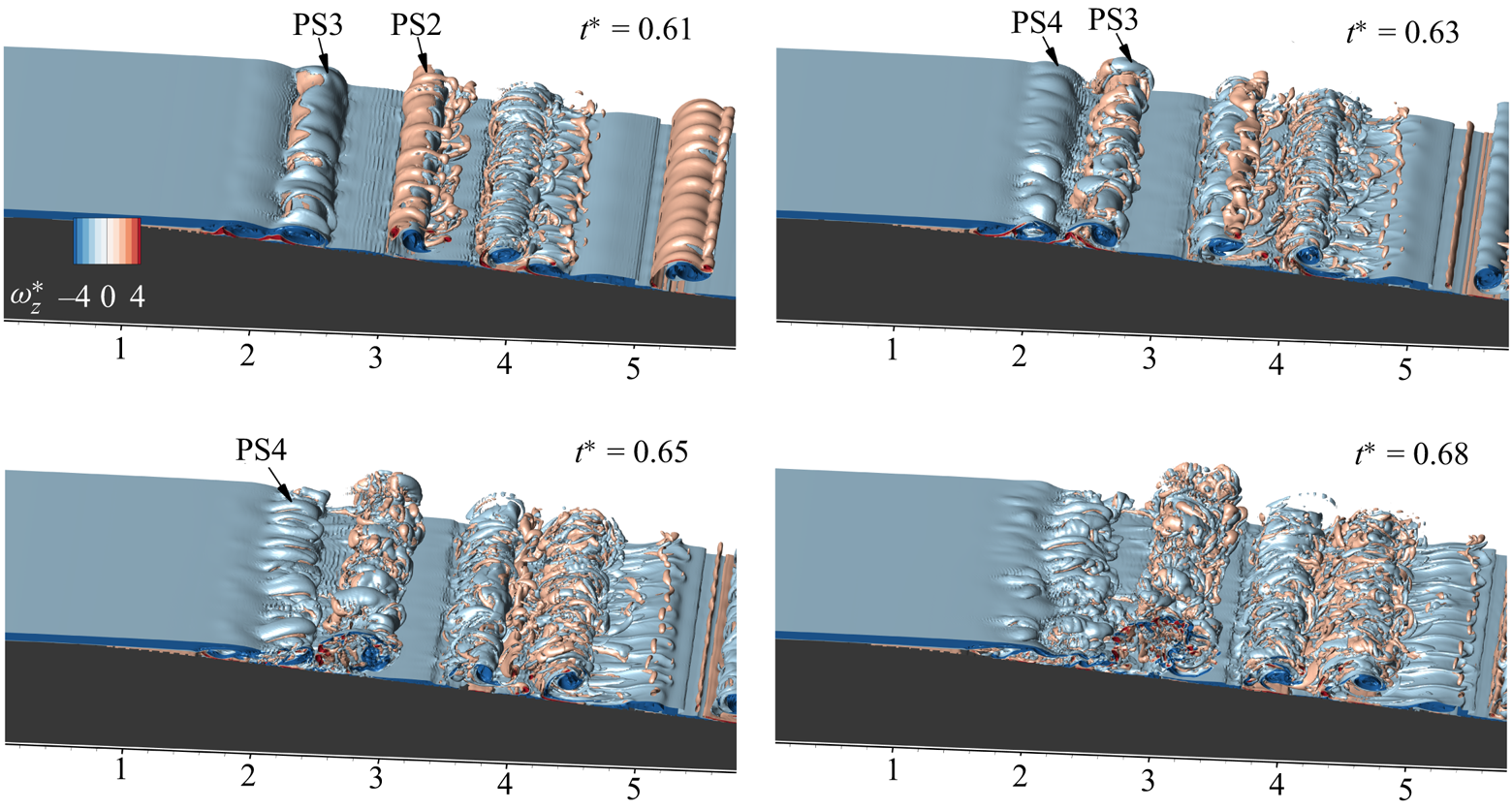
Figure 25. Three-dimensional disintegration of the separation bubble.
6.2. Shear layer shedding characteristics
In figure 26, the spanwise vorticity at a downstream location is probed to identify the temporal characteristics of the vortex shedding due to unsteady separation for cases C3 and D3. In case C3, vortex generation initiates around  $t^* = 0.3$, which is at an earlier flow instance than in case D3. Shortly after the vortex ejection, the formation of a positive vortex is evident by a sharp positive peak. Further oscillations are indicative of the subsequent formation and shedding of vortex structures. High-frequency perturbations in the zero mean inflow phase are triggered by three-dimensional fragmentation of the flow features in case C3. The vortex shedding in case D3 is more frequent and reveals a three-dimensional breakdown at an earlier stage in the flow. The underlying frequency of the vortex shedding is identified by the frequency spectra obtained from the Fourier transforms of the vorticity evolution. The highest peak in the frequency spectra obtained by the Fourier analysis indicates the shedding frequency and is marked in figure 26(b) for cases C3 and D3. A second dominant frequency lies close to the subsequent harmonics of the preceding dominant frequency in both cases.

Figure 26. Spectra analysis of vorticity probe for spatially unstable cases. (a) Temporal variation of spanwise vorticity (case C3,  $x = 2.633$, $y = 0.914$; case D3, $x = 2.32$, $y = 0.964$). (b) Frequency spectra of the spanwise vorticity variation.
The temporal characteristics of the periodic shedding of two-dimensional flow structures in type III cases are revealed by the DMD analysis of two-dimensional snapshots of spanwise vorticity. Unlike the former category cases, rapid evolution and the streamwise advection of flow features due to the low deceleration rate hinders the three-dimensional DMD analysis of streamwise vorticity. A total of 75 snapshots lying in the initial deceleration period between  $t_i$ and $t_f$ are used for the DMD analysis for both cases, with time step $\Delta \tau =2 \times 10^{-2}$. Frequency was invariant when the number of snapshot sizes was increased. Figure 27 summarizes the DMD analysis of the spanwise vorticity in spatially unstable cases. Typically, the Ritz circles plotted in figures 27(a) and 27(b) indicate the stability of DMD modes. The red symbols indicate the growing modes of cases C3 and D3 that lie outside the unit circle. To further emphasize the destabilizing nature, figures 27(c) and 27(d) present bar diagrams of frequency ( $\,f_{DMD}$) plotted against the growth rate ( $\sigma$) determined using DMD analysis. In each case, $1_{\sigma }$ denotes the most unstable mode based on the growth rate criteria. Growth rates and frequency information for each mode are provided in each figure. Figures 27(e) and 27(f) display the most prominent (highest growth rate) mode for cases C3 and D3, respectively. The peak frequencies of both modes are higher in the high Reynolds number case D3. Invariably, the first mode represents the growth of the vortex from the separation bubble over the diverging channel. A second dominant mode holds a frequency nearly equal to the second harmonic, indicating the second dominant peak of the vorticity frequency spectra (figures 27g,h). An alternate pattern in the second mode indicates the spanwise vortex roll-ups over the diverging region. In case D3, early vortex development leads to continuous shedding mode, as shown in figure 27(h). DMD results also point to the vortex shedding from the separation bubble in this period. Both analyses indicate two-dimensional vortex shedding characteristics, which later disintegrate three-dimensionally during the zero mean inflow phase.

Figure 27. DMD analysis of spanwise vorticity evolution: (a) Ritz circle (case C3), (b) Ritz circle (case D3). Frequency versus growth rate: (c) case C3, (d) case D3. (e) First mode, case C3, (f) first mode, case D3, (g) second mode, case C3, and (h) second mode, case D3).
A consolidated comparison of temporal characteristics obtained from frequency spectra with the results from DMD analysis is included in table 3. An average displacement thickness is calculated for the velocity profiles over the separation point and is denoted as  $\delta _{avg}^*$. Similarly, an average velocity is calculated by taking the mean of the average velocity of velocity profiles over the separation point (between $t_i$ and $t_f$). The Strouhal number ( $St = {f\delta _{avg}^*}/{U_{avg}}$) is calculated for both probe analysis and DMD analysis by using the average displacement thickness along with the average velocity. In the present study, the unstable mode frequency scales with the viscosity length scales generally used in boundary layer transition studies (Klebanoff, Cleveland & Tidstrom Reference Klebanoff, Cleveland and Tidstrom1992; Bakchinov et al. Reference Bakchinov, Grek, Klingmann and Kozlov1995), and identified Strouhal frequencies lie near $0.2$. In light of the fact that only 2 out of 12 cases show periodic vortex shedding, the results are insufficient to support the generalization of the Strouhal number relation.
Table 3. Temporal characteristics of vortex shedding due to unsteady separation.

7. Conclusion
We have investigated numerically the onset of turbulence in APG boundary layer conditions in a diverging channel by imposing the analytical solution of trapezoidal mean flow condition at the inlet of the computational domain to mimic the experimental conditions of Das et al. (Reference Das, Srinivasan and Arakeri2016). The effects of flow Reynolds numbers and deceleration Reynolds numbers are investigated systematically by varying the flow velocity and deceleration rate. The flow transition initiates with the thickening of the boundary layer followed by two-dimensional primary inflectional instability, which generally occurs in the deceleration phase and subsequently leads to flow separation and shear layer roll-up in the diverging section. Top wall boundary layers also exhibit inflectional instability, resulting in vortex roll-ups identical to the bottom wall in later flow instances. At low and medium Reynolds numbers, shear layer vortices remain two-dimensional, while secondary instabilities initiate the formation of three-dimensional structures at high Reynolds numbers. Based on the critical flow time flow associated with the initiation of secondary instability and temporally averaged streamwise vorticity, we have classified the flow evolution into three categories.
The first category (type I) occurs in low and moderate Reynolds number cases, which exhibit two-dimensional flow evolution of vortex flow structures that advect and diffuse during the zero mean inflow phase. The boundary layer growth occurs rapidly at high deceleration rates, whereas the increase is gradual at low deceleration rates. However, the time of flow separation and the vortex formation depend on the local Reynolds number based on the displacement thickness ( $Re_{\delta }^* \approx 600$ and 700, respectively). The emergence of the primary vortices leads to a progressive increase in circulation in the initial stage; after reaching a maximum during deceleration, the total circulation in the diverging section declines as the wall vortices diminish and spanwise vorticity decreases. The vortex structures maintain their two-dimensional nature during the zero inflow phase, whereas the individual vorticity magnitude of primary vortices decreases by the vortex decay.
In the second category (type II), a locally turbulent flow structure is evolved during the zero mean inflow phase ( $t^*_{3D} > 1$) by the amplification of the spanwise oscillation induced over the secondary vortex ejecting from the bottom wall. Similar to the former category, the boundary layer grows temporally, and higher inflow velocity in these cases leads to higher Reynolds numbers based on displacement thickness for flow separation ( $Re_\delta ^* \approx 940$) and vortex formation ( $Re_\delta ^* \approx 1070$). In addition to identifying the structure of the secondary instability using the $\lambda _2$ criteria, we also observed alternate streamwise vorticity developing over oscillations with an equivalent spanwise wavelength, which is identical to the features of the elliptic instability developing in a counter-rotating pair. We obtained additional information on the topology of unstable coherent flow structures with comparable wavelengths by taking the mode with the highest growth rate from the three-dimensional DMD analysis of streamwise vorticity. The instability characteristics of the secondary vortex are investigated further by calculating the growth rate theoretically using the parameters obtained from a Lamb–Oseen vorticity distribution identical to the vorticity distribution of the vortex pair ejected from the bottom wall as calculated by Leweke et al. (Reference Leweke, Le Dizes and Williamson2016). In cases with a locally unstable secondary vortex, the first Kelvin mode indicates an unstable nature, whereas the same analysis indicates a stable vortex pair for former category cases (type I).
The third category (type III) is characterized by low deceleration and high inflow velocity, which result in multiple shear layer roll-ups over the diverging section, and vortex shedding due to unsteady separation from the initial diverging section during the deceleration phase ( $t^*_{3D} < 1$). Identical to elliptic instability formation in the previous category, the three-dimensional visualizations of the spanwise vorticity indicate an oscillating secondary vortex in the vortex pair ejected from the initial diverging section during the deceleration phase. Low deceleration induces a higher advective velocity for flow structures, causing the spanwise vorticity roll-ups to pair over the diverging section, similar to the pairing of co-rotating vortices as described in Rogers & Moser (Reference Rogers and Moser1992). A separation bubble, comprising spanwise vorticity rolls with opposite sense of rotations developed due to unsteady separation, disintegrates at the end of the deceleration phase and compares well with the observations of Wissink & Rodi (Reference Wissink and Rodi2006). From DMD analysis, the most unstable mode identified by the highest growth rate exhibits an alternating pattern of spanwise vorticity, which indicates vortex shedding due to unsteady separation. Also, DMD analysis of spanwise vorticity yields frequency spectra that are in good agreement with probe analysis of vorticity evolution.
Declaration of interests
The authors report no conflict of interest.
Data availability statement
The data that support the findings of this study are available from the corresponding author upon reasonable request.
Appendix A. Inlet velocity profile – analytical solutions
For a unidirectional incompressible transient fluid flow without any body forces, the momentum equation in the streamwise direction reduces to
 \begin{equation} \frac{\partial u}{\partial t} =-\frac{1}{\rho}\left(\frac{\partial P}{\partial x} \right) + \nu \left(\frac{\partial^2 u}{\partial y^2} \right), \end{equation}
with the boundary conditions defined as
 $$\begin{gather} u(h,t) = u(-h,t) = 0 \quad (\text{no-slip}), \end{gather}$$
 $$\begin{gather}u(y,0) = 0, \quad \frac{\partial(u(0,t))}{\partial y} =0, \end{gather}$$
 $$\begin{gather}\int_0^h u(y,t)\,{\rm d}y = u_p(t)\,h. \end{gather}$$
 Analytical solution of fully developed laminar pulsating flow for variant volumetric flow rate is obtained by converting (taking Laplace transform) governing partial differential equations (A1)–(A4) with variable  $u(x,t)$ into an ordinary differential equation. The ordinary differential equation is solved for $\tilde {u}(x, s)$, and the function is inverted to yield $u(x, t)$ using the Bromwich integral formula. For single pulse cases, the analytical solutions are
 \begin{equation}
\left.\begin{aligned}\text{for} \quad 0\leq t&\leq
t_0,\\ &\quad\frac{u}{U_p}=\frac{1}{t_0}\left(A_1 t
-\frac{K A_2}{40} \right)-\frac{2
K}{t_0}\sum_{nh=1}^{\infty} \left(
\exp{\left(\frac{-v_{nh}^2
t}{K}\right)}\right) \times \varPsi, \\
\text{for} \quad t_0\leq t&\leq t_1,\\
&\quad\frac{u}{U_p}=A_1 -\frac{2 K}{t_0}\sum_{nh=1}^{\infty}
\left( \exp{\left(\frac{-v_{nh}^2
t}{K}\right)}-\exp{\left(\frac{-v_{nh}^2(t-t_0)
}{K}\right)}\right)\times \varPsi, \\
\text{for} \quad t_1\leq t&\leq t_2, \\ &\quad\frac{u}{U_p}=A_1
\left(\frac{t_2-t}{t_2-t_1}\right) +\frac{K A_2}{40 (t_2-t_1)}\\
&\quad\qquad\ \ -2 K
\sum_{nh=1}^{\infty}\left(\frac{\exp{\left(\dfrac{-v_{nh}^2
t}{K}\right)}-\exp{\left(\dfrac{-v_{nh}^2 (t-t_0)}
{K}\right)}}{t_0}-\dfrac{\exp{\left(\dfrac{-v_{nh}^2
(t-t_1)} {K}\right)}}{t_2-t_1}\right) \times
\varPsi, \\
&\text{for} \quad t> t_2, \\
&\quad\frac{u}{U_p}=- 2 K \sum_{nh=1}^{\infty}
\left(\frac{\exp{\left(\dfrac{-v_{nh}^2 t}{K}\right)}
-\exp{\left(\dfrac{-v_{nh}^2 (t-t_0)}{K}\right)}}
{t_0}\right.\\ &\qquad\quad\ \left. {}+\frac{\exp{\left(\dfrac{-v_{nh}^2
(t-t_2)}{K}\right)} -\exp{\left(\dfrac{-v_{nh}^2
(t-t_1)}{K}\right)}} {t_2-t_1}\right) \times
\varPsi, \\ & {\rm where} \quad
A_1=\frac{3}{2}(1-c_h ^2 ),\quad A_2 =5 c_h ^4 -6 c_h ^2 +1 ,\quad K=\frac{h^2}{\nu}, \\ &\qquad\quad\quad \, \, \, \, \varPsi =
\left[\frac{\cos(c_h
v_{nh})-\cos(v_{nh})}{v_{nh}^3\sin(v_{nh})}\right].
\end{aligned}\right\}
\end{equation}
\begin{equation}
\left.\begin{aligned}\text{for} \quad 0\leq t&\leq
t_0,\\ &\quad\frac{u}{U_p}=\frac{1}{t_0}\left(A_1 t
-\frac{K A_2}{40} \right)-\frac{2
K}{t_0}\sum_{nh=1}^{\infty} \left(
\exp{\left(\frac{-v_{nh}^2
t}{K}\right)}\right) \times \varPsi, \\
\text{for} \quad t_0\leq t&\leq t_1,\\
&\quad\frac{u}{U_p}=A_1 -\frac{2 K}{t_0}\sum_{nh=1}^{\infty}
\left( \exp{\left(\frac{-v_{nh}^2
t}{K}\right)}-\exp{\left(\frac{-v_{nh}^2(t-t_0)
}{K}\right)}\right)\times \varPsi, \\
\text{for} \quad t_1\leq t&\leq t_2, \\ &\quad\frac{u}{U_p}=A_1
\left(\frac{t_2-t}{t_2-t_1}\right) +\frac{K A_2}{40 (t_2-t_1)}\\
&\quad\qquad\ \ -2 K
\sum_{nh=1}^{\infty}\left(\frac{\exp{\left(\dfrac{-v_{nh}^2
t}{K}\right)}-\exp{\left(\dfrac{-v_{nh}^2 (t-t_0)}
{K}\right)}}{t_0}-\dfrac{\exp{\left(\dfrac{-v_{nh}^2
(t-t_1)} {K}\right)}}{t_2-t_1}\right) \times
\varPsi, \\
&\text{for} \quad t> t_2, \\
&\quad\frac{u}{U_p}=- 2 K \sum_{nh=1}^{\infty}
\left(\frac{\exp{\left(\dfrac{-v_{nh}^2 t}{K}\right)}
-\exp{\left(\dfrac{-v_{nh}^2 (t-t_0)}{K}\right)}}
{t_0}\right.\\ &\qquad\quad\ \left. {}+\frac{\exp{\left(\dfrac{-v_{nh}^2
(t-t_2)}{K}\right)} -\exp{\left(\dfrac{-v_{nh}^2
(t-t_1)}{K}\right)}} {t_2-t_1}\right) \times
\varPsi, \\ & {\rm where} \quad
A_1=\frac{3}{2}(1-c_h ^2 ),\quad A_2 =5 c_h ^4 -6 c_h ^2 +1 ,\quad K=\frac{h^2}{\nu}, \\ &\qquad\quad\quad \, \, \, \, \varPsi =
\left[\frac{\cos(c_h
v_{nh})-\cos(v_{nh})}{v_{nh}^3\sin(v_{nh})}\right].
\end{aligned}\right\}
\end{equation}Here,  $h$ is the channel half-height, $y$ is the distance from the centreline towards the wall of the channel, $c_h ={y}/{h}$, and $v_{nh}$, $nh = 1,2,3,\ldots, \infty$, are roots of $\tan (v) =v$. The first 50 roots of $\tan (v) =v$ are used to obtain the sum of the above converging infinity series.


 Open access