


1. Introduction
One fascinating phenomenon of sediment transport is the formation of patterns, such as ripples, dunes or ridges. These sediment patterns have important implications for many environmental and industrial applications, for example, they influence the rate of sediment transport in a given river. Although the problem of sediment pattern formation has been subject to extensive studies over the past several decades, a number of fundamental questions still remain unanswered due to the inherently complex dynamics (Best Reference Best2005; Andreotti & Claudin Reference Andreotti and Claudin2013; Charru, Andreotti & Claudin Reference Charru, Andreotti and Claudin2013). A key challenge is the accurate description of the driving turbulent flow over the bedforms and its interplay with the sediment bed. In particular, faithful description of the spatial structure of the boundary shear stress and its relation to the sediment flux remains an open problem. The latter defines the morphological evolution process of sedimentary patterns and is an important ingredient in many sediment transport models (Seminara Reference Seminara2010; Charru et al. Reference Charru, Andreotti and Claudin2013).
The present work is concerned with statistically two-dimensional transverse subaqueous bedforms worked by a uni-directional turbulent flow. The flow evolving over such train of bedforms is statistically non-homogeneous and entails complex interaction with the sediment bed (see e.g. review by Best Reference Best2005). To simplify the problem, most of previous experimental and numerical studies of the configuration have considered flow over fixed dunes with imposed geometry (see e.g. McLean & Smith Reference McLean and Smith1986; Nelson, McLean & Wolfe Reference Nelson, McLean and Wolfe1993; McLean, Nelson & Wolfe Reference McLean, Nelson and Wolfe1994; Bennett & Best Reference Bennett and Best1995; Stoesser et al. Reference Stoesser, Braun, García-Villalba and Rodi2008; Omidyeganeh & Piomelli Reference Omidyeganeh and Piomelli2011). Although such studies have been useful in elucidating the key features of the flow, they fail to provide information on the mutual interaction between the flow and the evolving sediment bed composed of mobile grains. Similarly, theoretical studies that investigate the hydro-morphodynamic instability and evolution of the sediment bed invoke a disparity in time scales between the flow and the bed shape evolution and assume a fixed wavy bottom perturbation to solve the fluid flow (see e.g. Kennedy Reference Kennedy1963; Richards Reference Richards1980; Colombini & Stocchino Reference Colombini and Stocchino2011). Customarily, the flow solution is based on the seminal work by Jackson & Hunt (Reference Jackson and Hunt1975), which is an extension of the asymptotic solutions of the laminar flow over a bump by Benjamin (Reference Benjamin1959) to the turbulent regime (see reviews by Belcher & Hunt (Reference Belcher and Hunt1998) and Charru et al. (Reference Charru, Andreotti and Claudin2013) for a detailed account). An important outcome of these studies is that the flow can be considered as a layered structure: an outer inviscid region far from the bottom and an inner ‘logarithmic’ region where turbulent stresses and viscosity are important. In the theoretical analysis, the matching of the two layers reveals a phase advance of the boundary shear stress with respect to the topography. In the context of sediment transport, the phase difference between the shear stress and the bottom is the main destabilising mechanism of a perturbed erodible bed. A balance between this destabilising mechanism and other stabilising effects such as gravity (Engelund & Fredsoe Reference Engelund and Fredsoe1982) and sediment-bed relaxation effects (Charru Reference Charru2006; Fourrière, Claudin & Andreotti Reference Fourrière, Claudin and Andreotti2010) is believed to result in the initiation of bed patterns at a certain preferred wavelength. However, finite-amplitude effects beyond the linear regime, such as flow separation downstream of the ripple crest, cannot be accounted for by the above methods and a theoretical description is still an open issue (Charru & Luchini Reference Charru and Luchini2019).
Concerning the sediment bed, the majority of the algebraic models that relate the fluid shear stress with the sediment flux are developed for the equilibrium state. The transient behaviour of the sediment bed is usually treated by assuming that the bed responds to changes in flow conditions instantaneously. This assumption allows one to relate the local shear stress to the local particle flow rate. However, it is well recognised that the sediment bed needs some temporal/spatial lag to adapt to a change in the flow conditions due to its inertia (Sauermann, Kroy & Herrmann Reference Sauermann, Kroy and Herrmann2001; Charru Reference Charru2006). The sediment-bed relaxation behaviour, usually expressed in terms of a characteristic saturation length scale, has been argued to be a stabilising factor during sediment-bed instability and it thereby controls the scaling of initial aeolian/subaqueous bedforms. Although models that include such a sediment relaxation effect through the introduction of a separate differential equation for the particle number density or for the particle flux (Valance Reference Valance2005; Charru Reference Charru2006; Fourrière et al. Reference Fourrière, Claudin and Andreotti2010) into the stability analysis have been partially successful, they still fall short of accurately determining the initial ripple wavelength (Langlois & Valance Reference Langlois and Valance2007; Ouriemi, Aussillous & Guazzelli Reference Ouriemi, Aussillous and Guazzelli2009). The limitation is attributed to the lack of a fully appropriate model for the saturation length that stems from the simplified description of the complex particle dynamics near and inside the bed. Moreover, the two-way feedback mechanism between the sediment grains and the shearing flow is usually ignored. The saturation length encompasses a wide spectrum of length scales as a consequence of simultaneously occurring particle transport modes (rolling, sliding, saltation, etc.) and dynamical mechanisms (rebounding, inter-particle collision, particle–turbulence interaction, etc.). A dominant transport mode or mechanism is usually selected for a given regime. For instance, in the particle inertia dominated regime, the relaxation is believed to scale with the drag length  $l_d$, which is often based on Stokes drag, i.e. $l_d \approx (\rho _p/\rho _f)D$, where $\rho _p/\rho _f$ and $D$ are the fluid-to-particle density ratio and particle diameter, respectively (Fourrière et al. Reference Fourrière, Claudin and Andreotti2010). Other saturation length models account for different hydrodynamic and granular bed interactions and introduce other length scales, such as the deposition length that represents the distance travelled by particles (moving at a certain characteristic velocity), during their deposition time $t_d \sim D/u_s$, where $u_s$ is the particle settling velocity (Charru & Hinch Reference Charru and Hinch2006; Charru Reference Charru2006). In the context of aeolian sand transport (very large particle-to-fluid density ratios), the saltation length, which represents the distance covered by saltating grains during their flight time, is considered to be the governing length scale (Sauermann et al. Reference Sauermann, Kroy and Herrmann2001). In an attempt to address the above shortcomings, Pähtz et al. (Reference Pähtz, Kok, Parteli and Herrmann2013, Reference Pähtz, Parteli, Kok and Herrmann2014, Reference Pähtz, Omeradžić, Carneiro, Araújo and Herrmann2015) propose a more elaborate and fairly complex model with several adjustable parameters that accounts for additional mechanisms such as the relaxation associated with the fluid–particle and inter-particle interactions.
Carrying out highly resolved experimental measurements of both the flow and the erodible sediment-bed motion (in the presence of bedforms) is a difficult task and available data are scarce (see e.g. Charru & Franklin Reference Charru and Franklin2012; Rodrıguez-Abudo & Foster Reference Rodrıguez-Abudo and Foster2014; Leary & Schmeeckle Reference Leary and Schmeeckle2017; Frank-Gilchrist, Penko & Calantoni Reference Frank-Gilchrist, Penko and Calantoni2018). Notably, Charru & Franklin (Reference Charru and Franklin2012) report measurements of the flow over isolated evolving barchan dunes in a confined channel flow experiment. They assessed the layered structure of the flow over the barchan as predicted by the asymptotic theories, ignoring the re-circulating flow downstream of the barchan brink (measurements of the three-dimensional flow were taken at the symmetry plane of the barchan). However, the experiments did not allow access to the relationship between the local shear stress and the particle flux. Concerning the sediment-bed relaxation behaviour, there is currently no direct experimental measurement of the saturation length for subaqueous sediment transport available (Andreotti & Claudin Reference Andreotti and Claudin2013; Duran Vinent et al. Reference Duran Vinent, Andreotti, Claudin and Winter2019). The majority of field and laboratory measurements as well as theoretical modelling of the saturation length have been for the aeolian sediment transport regime (Andreotti, Claudin & Douady Reference Andreotti, Claudin and Douady2002; Lajeunesse, Malverti & Charru Reference Lajeunesse, Malverti and Charru2010; Claudin, Wiggs & Andreotti Reference Claudin, Wiggs and Andreotti2013; Pähtz et al. Reference Pähtz, Omeradžić, Carneiro, Araújo and Herrmann2015; Selmani et al. Reference Selmani, Valance, Ould El Moctar, Dupont and Zegadi2018; Gadal et al. Reference Gadal, Narteau, Ewing, Gunn, Jerolmack, Andreotti and Claudin2020; Lü et al. Reference Lü, Narteau, Dong, Claudin, Rodriguez, An, Fernandez-Cascales, Gadal and Courrech du Pont2021). In these studies, saturation length measurements are reported by retrieving the grain flux indirectly from the measurement of bed elevation profiles through the sediment mass conservation equation.
Faithful numerical simulation of sediment transport phenomena is very challenging. It has thus been common practice to simplify the description of the flow and/or the sediment-bed dynamics. On the one hand, there are studies that fully resolve the turbulent flow while describing the sediment bed via continuum modelling (see e.g. Chou & Fringer Reference Chou and Fringer2010; Khosronejad & Sotiropoulos Reference Khosronejad and Sotiropoulos2014; Zgheib et al. Reference Zgheib, Fedele, Hoyal, Perillo and Balachandar2018; Zgheib & Balachandar Reference Zgheib and Balachandar2019) or via point-particle based Lagrangian modelling (Finn, Li & Apte Reference Finn, Li and Apte2016; Guan et al. Reference Guan, Salinas, Zgheib and Balachandar2021). Other studies, on the other hand, sufficiently account for the dynamics of the sediment bed (based on discrete-element models) but without resolving the turbulent background flow (Durán, Andreotti & Claudin Reference Durán, Andreotti and Claudin2012; Schmeeckle Reference Schmeeckle2014; Maurin et al. Reference Maurin, Chauchat, Chareyre and Frey2015). Both modelling approaches rely on some sort of (semi-)empirical expression to couple the fluid problem with the morphodynamic one. Recent progress in particle-resolving direct numerical simulations (DNS) that account for both the flow and individual grain motion without modelling the fluid–particle interaction have started to shed light on the grain-scale dynamics and the interaction of an evolving thick sediment bed with the driving turbulent flow (see e.g. Kidanemariam & Uhlmann Reference Kidanemariam and Uhlmann2014a; Vowinckel, Kempe & Fröhlich Reference Vowinckel, Kempe and Fröhlich2014; Kidanemariam Reference Kidanemariam2015; Kidanemariam & Uhlmann Reference Kidanemariam and Uhlmann2017; Mazzuoli, Kidanemariam & Uhlmann Reference Mazzuoli, Kidanemariam and Uhlmann2019; Mazzuoli et al. Reference Mazzuoli, Blondeaux, Vittori, Uhlmann, Simeonov and Calantoni2020; Scherer, Kidanemariam & Uhlmann Reference Scherer, Kidanemariam and Uhlmann2020; Jain, Tschisgale & Fröhlich Reference Jain, Tschisgale and Fröhlich2021).
The objective of the present work is to investigate, with the aid of particle-resolved DNS data, the spatial structure of the turbulent flow and the particle motion over a train of two-dimensional transverse bedforms, and to address its correlation with the evolving sediment bed. In our recent work (Kidanemariam & Uhlmann Reference Kidanemariam and Uhlmann2017, hereafter termed as KU2017), we have carried out extensive simulations of subaqueous pattern formation in a turbulent open-channel flow configuration. The study in KU2017 was devoted to the initiation and evolution aspects of the sediment patterns. In the present contribution, we revisit the simulation data in KU2017 and analyse the fluid flow and particle motion. In particular, we analyse the spatial structure of the bed shear stress and its relation to the particle flow rate. To this end, we have performed ripple-conditioned phase averaging of the fluid flow that takes into account the spatio-temporal variability of the sediment bed. Let us note that the conditions of the simulations reported in KU2017 (varying the computational box size for a single physical parameter point) allowed systematic investigation of the different ripple evolution stages. That is, the temporal growth of the ripple size was systematically ‘frozen’ by limiting the computational domain length that accommodates only a single ripple unit. The formed ripples were thereby constrained to migrate steadily, maintaining their asymmetric shape at a mean wavelength equal to the length of the domain. The strategy allows us to accumulate sufficient statistics for detailed analysis of the interaction between the turbulent flow and the evolving ripple unit. The paper is organised as follows: in § 2 we provide a short description of the computational set-up and numerical solution strategy. The evolution of the bulk flow characteristics in response to the evolution of the bed is presented in § 3. In § 4 we present phase-averaged statistics including that of the boundary shear stress and evaluate the phase lag between the bed shear stress and the sediment flux. The main findings of the paper are summarised and discussed in § 5.
2. Flow configuration, simulation strategy and numerical method
We consider an open-channel flow of an incompressible viscous fluid with a density  $\rho _f$ and viscosity $\nu$ over an evolving sediment bed, as shown schematically in figure 1. The sediment bed is composed of spherical particles of diameter $D$ and density $\rho _p$. A Cartesian coordinate system $(x, y, z)$ is defined, $x$ and $z$ representing the streamwise and spanwise (lateral) directions respectively while $y$ is the vertical direction. The corresponding Eulerian fluid and Lagrangian sediment particle velocity vectors are defined as ${\boldsymbol {u}_f} = (u_f,v_f,w_f)$ and ${{\boldsymbol {u}_p}} = (u_p,v_p,w_p)$, respectively. Mean flow is directed in the positive $x$ direction and the vector of gravitational acceleration ${{\boldsymbol {g}}}$ points in the negative $y$ direction. The mean fluid height is denoted as ${H_f}$ while the corresponding mean sediment-bed thickness is denoted as $H_b$.

Figure 1. Schematics of an open-channel flow of a fluid with density  $\rho _f$ and viscosity $\nu$ over an evolving sediment bed. The sediment bed is represented by a large number of freely moving spherical particles of diameter $D$ and density $\rho _p$.
The simulation data analysed in the present study are identical to those reported in KU2017. Specifically, data corresponding to the ripple featuring cases termed  ${\rm H}4^{3}$, H6 and H7 therein, are considered for the phase-averaging analysis. Details of the simulation campaign and numerical method used can be found in KU2017. A short description is provided here for completeness. The simulations were carried out in bi-periodic three-dimensional computational boxes (periodic in the streamwise and spanwise directions). No-slip and free-slip conditions were imposed at the bottom and top planes of the channel, respectively. The flow was driven by a streamwise pressure gradient imposing a desired constant mean flow rate ${{q_f}}$. The fluid flow is described by the bulk Reynolds number ${{Re_b}} = {{u_b}} {H_f}/\nu$ or equivalently the friction Reynolds number ${{Re_\tau }} = u_{\tau } {H_f}/\nu$, where ${{u_b}} \equiv {{q_f}}/{H_f}$ and $u_{\tau }$ are the bulk and friction velocities respectively. Note that $u_{\tau }$ is evaluated a posteriori from the mean total shear stress evaluated at a wall-normal location of the mean fluid–bed interface $y = H_b$. The location of the interface between the fluid and the sediment bed has been determined based on the threshold value of the solid volume fraction. Details of the extraction of the fluid–bed interface and precise definitions of ${H_f}$, $H_b$ and $u_{\tau }$ can be found in KU2017. Important parameters describing the submerged sediment bed include: the particle-to-fluid density ratio $\rho _p/\rho _f$, the length scale ratios ${H_f}/D$ and $D^{+}\equiv Du_{\tau }/\nu$ and a ratio between the gravity and viscous forces described by the Galileo number ${{Ga}} = U_gD/\nu$, where $U_g$ is the gravitational velocity scale $U_g = \sqrt {(\rho _p/\rho _f-1)|\boldsymbol {g}|D}$. Finally, let us define the Shields number, which is the ratio between the fluid shear force at the bed and the submerged weight of a particle, as
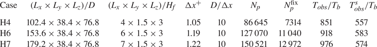
  $\theta \equiv (u_{\tau }/U_g)^{2}$ (Shields Reference Shields1936). The values of these physical parameters are listed in table 1. Note that the three simulation cases have identical values of the imposed physical parameters. As shown in table 2, the only difference, in terms of imposed quantities, is the streamwise extent of the simulation box. Case H4 has a domain length of approximately four times the mean fluid height, while that of H6 and H7 is approximately six and seven times the mean fluid height, respectively. These differences in domain length result in different sizes of the accommodated ripple units that in turn result in somewhat different values of the derived parameters such as ${{Re_\tau }}$, $\theta$ and $D^{+}$ (the evolution process is discussed in more detail in § 3).
Table 1. Physical parameters of the simulations;  ${{Re_b}}$ and ${{Re_\tau }}$ are the bulk and friction Reynolds numbers, respectively; $\rho _p/\rho _f$ is the particle-to-fluid density ratio; ${{Ga}}$ and $\theta$ are the Galileo number and the Shields number, respectively.

Table 2. Numerical parameters of the simulations;  $L_i$ is the domain length in the $i$th direction. The grid spacing is uniform in all directions, i.e. $\Delta x = \Delta y = \Delta z$; $N_p$ is the number of particles in the simulations, out of which $N_{p}^{fix}$ are fixed in space at the channel bottom to create a rough boundary; $T_{obs}$ is the total observation time of each simulation starting from the release of the moving particles. Ripple-conditioned statistics are computed over the steady dune propagation interval $T^{s}_{obs}$; $T_b = {H_f}/{{u_b}}$ is the bulk time unit.
The numerical method used to carry out the simulations is based upon the immersed boundary technique of Uhlmann (Reference Uhlmann2005) for the treatment of the fluid–solid interactions, wherein the incompressible Navier–Stokes equations are solved with a second-order finite-difference method throughout the entire computational domain, adding a localised force term that serves to impose the no-slip condition at the fluid–solid interface. Individual sediment particle motion is obtained via integration of the Newton–Euler equations for rigid body motion, driven by the hydrodynamic force (and torque) as well as gravity and the force (torque) resulting from solid–solid contact. The inter-particle collision process is described via a discrete element model (DEM) based on the soft-sphere approach (Kidanemariam & Uhlmann Reference Kidanemariam and Uhlmann2014b). A pair of particles is defined as ‘being in contact’ when the smallest distance between their surfaces,  $\varDelta$, becomes smaller than a force range $\varDelta _c$. The resulting contact force is then the sum of an elastic normal component, a normal damping component and a tangential frictional component. The elastic part of the normal force component is a linear function of the penetration length $\delta _c \equiv \varDelta _c-\varDelta$, with a stiffness constant $k_n$. The normal damping force is a linear function of the normal component of the relative velocity between the particles at the contact point with a constant coefficient $c_n$. The tangential frictional force (the magnitude of which is limited by the Coulomb friction limit with a friction coefficient $\mu _c$) is a linear function of the tangential relative velocity at the contact point, again formulated with a constant coefficient denoted as $c_t$. Since the characteristic collision time is typically orders of magnitude smaller than the time step of the flow solver, the numerical integration of the equations for the particle motion is carried out adopting a sub-stepping technique, freezing the hydrodynamic forces acting upon the particles between successive flow field updates. A detailed description of the collision model and the corresponding parameter values as well as extensive validation and convergence studies can be found in Kidanemariam & Uhlmann (Reference Kidanemariam and Uhlmann2014b).
3. Evolution of the flow and sediment bed
The simulations were initiated by first developing a turbulent flow over a macroscopically flat bed composed of pseudo-randomly packed stationary particles. The coupled fluid–solid simulations were then switched on by allowing the particles to move (except the  $N_{p}^{fix}$ particles that are fixed in space at the channel bottom to create a rough boundary). Subsequently, the macroscopically flat sediment bed gets perturbed as a result of the ensuing particle erosion and deposition processes caused by the shearing turbulent flow above. For the conditions of our simulations, the sediment-bed perturbations ultimately evolve towards statistically two-dimensional transverse bedforms that propagate downstream at a constant migration velocity and with a wavelength equal to the domain length. The bed evolution in turn modifies the flow from its initial statistically one-dimensional state towards a two-dimensional flow with strong spatio-temporal correlation with the morphology of the underlying bed. Let us first look at the evolution of bulk sediment and fluid flow properties. In figure 2(a), we reproduce from KU2017 the temporal evolution of the root-mean-square (r.m.s.) sediment-bed height $\sigma _{h}$ for the three cases considered in the present study (for reference, the evolution of the featureless bedload transport case H3 is also plotted). After an initial exponential growth, $\sigma _{h}$ attains a statistically constant value. The corresponding temporal evolution of the instantaneous friction Reynolds number ${{Re_\tau }}^{i}$ is also provided in figure 2(b). Here, ${{Re_\tau }}^{i}$ is computed from the instantaneous value of the imposed driving pressure gradient $\varPi$ that is required to maintain the desired constant flow rate. The latter is obtained from the integration of the streamwise momentum equation across the whole computation domain that, subject to the incompressibility constraint, reduces to
 \begin{equation} \varPi(t) ={-} \frac{1}{L_xL_yL_z} \sum_{l=1}^{N_{p}} I_{fix}^{(l)}({F}^{H(l)}_{p,x}(t) + {F}^{C(l)}_{p,x}(t)) - \frac{1}{L_y}\langle \tau^{W}\rangle_{xz}(t), \end{equation}
where  ${F}^{H(l)}_{p,x}$ and ${F}^{C(l)}_{p,x}$ are the streamwise components of the hydrodynamic and collision forces acting on the $l$th particle, respectively. Here, $I_{fix}^{(l)}$ is an indicator function that has a value of unity if the $l$th particle is held fixed and zero otherwise; $\langle \tau ^{W}\rangle _{xz}$ is the instantaneous average shear stress at the bottom smooth wall beneath the stationary particles and has a negligible contribution due to the practically zero velocity gradients therein. Thus, the driving volume force is is entirely balanced by the total resistance force exerted by the stationary particles located beneath the mobile sediment layer. The friction Reynolds number correspondingly increases from an initial value of ${{Re_\tau }}^{i}\approx 190$ to the average values $Re_\tau$ (measured in the asymptotic regime), as reported in table 1. Note that the initial ${{Re_\tau }}$ value corresponds to the turbulent flow over the macroscopically flat bed prior to the start of the coupled fluid–solid simulations. Since the total number of the heavier-than-fluid spherical particles remains the same during the simulation period, the average sediment-bed height remains essentially constant with time (except for some initial short dilation interval). Thus the temporal increase of ${{Re_\tau }}^{i}$ is entirely a consequence of the increasing roughness height of the bedforms. This is further confirmed by the direct correspondence of the evolution of the r.m.s. sediment-bed height and ${{Re_\tau }}^{i}$.

Figure 2. (a) Time evolution of the root-mean-square sediment-bed-height fluctuation normalised by the particle diameter (data reproduced from KU2017). (b) The corresponding evolution of the instantaneous friction Reynolds number for each of the cases. The vertical dashed lines indicate the start time of the steady ripple propagation interval over which statistics are accumulated. The circle symbols along the  ${{Re_\tau }}$ evolution of case ${H6}$ correspond to the time instances of the visualisations in figure 3. (c) The hydrodynamic roughness length $k_0$ as a function of the mean sediment-bed-height fluctuation $\langle \sigma _{h}\rangle _t^{+}$. In all plots, lines and symbols are colour coded as follows: grey, featureless bedload; blue, H4; red, H6; black, H7.
One way of quantifying the feedback of the evolving sediment bed on the turbulent flow is to express the mean fluid velocity profile  $U_f$ in the logarithmic layer through the definition of a hydrodynamic roughness height $k_0$ as $U_f^{+} = 1/\kappa \log ((y-y_0)/k_0)$, where $\kappa =0.41$ is the von Kármán coefficient and $y_0$ is some reference origin (Jiménez Reference Jiménez2004). The majority of the available sediment morphodynamic models strongly depend on the roughness parameter $k_0$ (Charru et al. Reference Charru, Andreotti and Claudin2013) and make use of classical correlations of $k_0$ versus particle Reynolds number $D^{+}$ that are obtained, for example, from flows over stationary roughness elements (see e.g. Fourrière et al. Reference Fourrière, Claudin and Andreotti2010; Colombini & Stocchino Reference Colombini and Stocchino2011; Duran Vinent et al. Reference Duran Vinent, Andreotti, Claudin and Winter2019). However, as is demonstrated in figure 2(c), the motion of the sediment bed and the evolving ripples substantially increase the value of $k_0$ for essentially the same value of $D^{+}$.
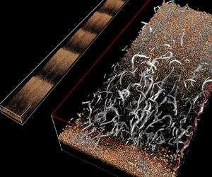
Figure 3 shows sample instantaneous flow visualisations of case H6 at selected times, spanning the duration from the first instants of the bed instability (several bulk time units after particles are released), through the initial evolution stage and up to the steady ripple propagation interval. The snapshots clearly highlight the coupled spatio-temporal evolution of the sediment bed and turbulent flow above. It can be seen that the intensity and density of the coherent structures evolve to be the highest in regions downstream of the crest of the forming transverse bedforms. It is the contrary for regions of the flow above and upstream of the crest where turbulence activity is weaker. The non-homogeneous spatial distribution of the vortices visually corroborates previous experimental and numerical investigation of the flow over fixed dunes (McLean et al. Reference McLean, Nelson and Wolfe1994; Stoesser et al. Reference Stoesser, Braun, García-Villalba and Rodi2008; Omidyeganeh & Piomelli Reference Omidyeganeh and Piomelli2011). It is known that the flow over developed two-dimensional bedforms possesses distinct regions that can be summarised into an accelerating and a decelerating flow region upstream and downstream of the dune crest respectively, a shear layer region downstream of the dune crest where flow separation occurs, a re-circulation region extending several dune heights downstream of the crest and bounded by the shear layer and a developing boundary layer region attached to the stoss side of the dune (Best Reference Best2005). The snapshots illustrate the complexity of the flow in this configuration. Moreover, the visualisations additionally show that large coherent structures leave their footprint in the morphology of the bed, visible as slight longitudinal ridges and troughs superposed on the transverse bedforms. The mechanism behind the formation of these ridges is equally fascinating (cf. Scherer et al. Reference Scherer, Uhlmann, Kidanemariam and Krayer2021) but is outside the scope of the present work.

Figure 3. Instantaneous snapshots of the flow field and particle positions of case H6 at times (a)  $t/T_b \approx 7$, (b) $t/T_b \approx 110$, (c) $t/T_b \approx 212$ and (d) $t/T_b \approx 423$. The top-view panels show turbulent vortical structures (grey surfaces) over the sediment-bed particles that are coloured based on their wall-normal location. The side-view panels show the corresponding spanwise vorticity on an $x$–
$x$– $y$ plane located at $z=0$ (the intersection region of particles and the plane is shown in black).
4. Ripple-conditioned fluid flow and particle motion
Here, we present an analysis of the turbulent flow field and particle motion that develops over the time-dependent sediment bed. We have performed ripple-conditioned phase averaging of the flow field in the steady ripple propagation interval. The reader is referred to Appendix A for the precise definition of the space- and time-averaging operators, while Appendix B details the phase averaging procedure and definition of notations used in subsequent sections.
4.1. Spatial structure of the mean flow
The streamwise and wall-normal components of the phase-averaged fluid velocity vector  $\tilde {\boldsymbol {U}}_f\equiv ({{\tilde {U}_f}},{{\tilde {V}_f}})$ and the corresponding particle velocity vector ${{\tilde {\boldsymbol {U}}_p}}\equiv ({{\tilde {U}_p}},{{\tilde {V}_p}})$ for case H7 are shown in figure 4 (cf. Appendix B for the definitions of $\tilde {\boldsymbol {U}}_f$ and ${{\tilde {\boldsymbol {U}}_p}}$). The figures highlight significant modulation of the flow by the ripple morphology. As is expected, below the fluid–bed interface, mean fluid and particle velocities are found to be negligibly small. Above the fluid–bed interface, on the other hand, velocities of both phases show large spatial variations that are seen to be strongly correlated with the ripple geometry. At and near the interface, ${{\tilde {U}_f}}$ is observed to be higher in the region above the crest of the ripple. The value of ${{\tilde {U}_f}}$ decreases downstream of the crest, attaining negative values in the re-circulation region highlighted by the negative ${{\tilde {U}_f}}$ contour shown in figure 4(a). Let us remark that a zero-valued contour level does not precisely demarcate the extent of the re-circulation region as there is very small but non-zero mean velocity inside the bed. The value of ${{\tilde {U}_f}}$ gradually increases along the ripple stoss side up to the crest. Similarly, in the outer flow region, ${{\tilde {U}_f}}$ exhibits higher velocity values in the flow contraction region above the crest and lower velocity values in the expansion region above the ripple stoss side. The wall-normal fluid velocity also exhibits an upward moving fluid region ( ${{\tilde {V}_f}}>0$) above the stoss side and a downward moving fluid region ( ${{\tilde {V}_f}}<0$) above the region downstream of the crest. A small region of positive ${{\tilde {V}_f}}$ is observed immediately downstream of the crest in the vicinity of the fluid–bed interface that corresponds to the up-lifting fluid of the re-circulation region. As $y$ tends to the upper boundary, ${{\tilde {V}_f}}$ tends to zero due to the imposed boundary condition.

Figure 4. (a) Phase-averaged fluid velocity components ( ${{\tilde {U}_f}}^{+},{{\tilde {V}_f}}^{+}$) of case H7. Contour levels of ${{\tilde {U}_f}}^{+},{{\tilde {V}_f}}^{+}= 0.1$ and $-0.1$ are marked by red and magenta curves. The phase-averaged sediment-bed height, ${\tilde {H}_b}$, is shown by the dashed curve. The vertical thin lines indicate the locations where wall-normal profiles of each quantity are extracted. (b) The corresponding phase-averaged particle velocity components ( ${{\tilde {U}_p}}^{+},{{\tilde {V}_p}}^{+}$). (c) Values of ${{\tilde {U}_f}}$ and ${{\tilde {U}_p}}$ extracted along the fluid–bed interface (shown by the curve at the top of the figure). The red dashed line represents the mean ripple migration velocity. (d) Same as panel (c) but for ${{\tilde {V}_f}}$ and ${{\tilde {V}_p}}$. (e) Wall-normal profiles ${{\tilde {U}_f}}$ and ${{\tilde {U}_p}}$ at selected streamwise locations. Profiles are, from left to right, at ${{\tilde {x}}}/D = 0$, $30$ and $112$ consecutively. The horizontal dashed lines indicate the location of the fluid–bed interface at the corresponding streamwise locations. ( f) Same as panel (e) but for ${{\tilde {V}_f}}$ and ${{\tilde {V}_p}}$.
The mean particle velocities also exhibit generally the same spatial structure as that of the fluid. From the intensity of the colour plots, it can be seen that the magnitude of streamwise particle velocity is on average smaller than that of the fluid in the region far above the fluid–bed interface, except in the re-circulation region. The opposite is true for the wall-normal component  ${{\tilde {V}_p}}$, which is observed to be higher in magnitude than that of the fluid. More quantitative comparison of the fluid and particle velocities can be inferred from the profiles along the location of the fluid–bed interface shown in figure 4(c,d) as well as from the wall-normal profiles of the same quantities at selected streamwise locations ${{\tilde {x}}}/D = 0$ (near crest), ${{\tilde {x}}}/D = 30$ (in trough) and ${{\tilde {x}}}/D = 112$ (on the stoss side of the ripple) shown in figure 4(e, f). It can be seen that the fluid/particle velocities strongly vary along the fluid–bed interface. Note that the fluid–bed interface is permeable and is subject to active mass and momentum exchange of both phases as a result of erosion, transport and deposition of sediment particles as well as the fluid motion therein. At the ripple crest the streamwise velocity of both phases reaches local maximum values of up to ${{\tilde {U}_f}}^{+}\approx 4$ and ${{\tilde {U}_p}}^{+} \approx 3$, whereas in the ripple troughs, velocities decrease considerably, attaining negative values in the re-circulation region. Further observation is that particles are on average moving at a smaller streamwise velocity than that of the fluid along the fluid–bed interface, except in the re-circulation region, where the opposite trend is observed. On the stoss side of the ripples, the value of the velocity lag between the two phases ranges between $1u_{\tau }$ and $1.5u_{\tau }$, whereas in the re-circulation region, a negative velocity lag of up to $-0.35u_{\tau }$ is observed. The origin of the velocity lag could be explained by the combined effect of the preferential distribution of inertial particles with respect to the near-wall high- and low-speed fluid regions (Kidanemariam et al. Reference Kidanemariam, Chan-Braun, Doychev and Uhlmann2013) and the fact that finite-sized particles feel the traction effect of neighbouring particles, which are located at a lower wall-normal location and are moving at a lower velocity, more than fluid particles do. Note that the particle velocity is much higher than the mean ripple migration velocity ${{u_{D}}}$ over the entire stoss side of the ripples, while the opposite is true at locations downstream of the crest. This observation is in line with the fact that ripples propagate as a result of erosion and deposition of sediment grains at the bed surface. ${{\tilde {V}_f}}$ and ${{\tilde {V}_p}}$ along the fluid–bed interface exhibit a notably different trend when compared with their streamwise counterparts. On the stoss side, ${{\tilde {V}_f}}$ and ${{\tilde {V}_p}}$ are positive while the difference between their values is not substantial. Moreover, the location of the local maximum of ${{\tilde {V}_f}}$ ( ${{\tilde {V}_p}}$) is observed to be located further upstream of the crest when compared with the streamwise components. Both phases exhibit an approximately zero value of the wall-normal velocity in the vicinity of the crest.
The wall-normal profiles of fluid and particle velocities presented in figure 4(e, f) further corroborate the above observations. Note that the apparent velocity lag is significant even at wall-normal locations well above the fluid–bed interface. Namely, positive velocity lag on the stoss side of the ripples ( ${{\tilde {U}_f}}>{{\tilde {U}_p}}$) and negative velocity lag in the re-circulation region ( ${{\tilde {U}_f}}<{{\tilde {U}_p}}$). In the region well above the fluid–bed interface, the preferential sampling of low-speed fluid regions by inertial particles (Kidanemariam et al. Reference Kidanemariam, Chan-Braun, Doychev and Uhlmann2013) is expected to be the dominant reason for the observed positive velocity lag. The negative velocity lag in the re-circulation region is again attributed to particle inertia. Sediment particles that are suspended from the crest with high momentum into the re-circulation region do not immediately adapt to the new environment, thus resulting in a statistically higher mean particle velocity than that of the fluid. Turning to the wall-normal velocity component, the profiles further highlight the mean positive and negative velocities upstream and downstream of ripple crests, respectively. Furthermore, upstream of the crest and above the fluid–bed interface, the particles’ wall-normal velocity is observed to be larger in magnitude than that of the fluid whereas downstream of the crest and above the fluid–bed interface, the particle velocity is observed to be substantially smaller (larger in absolute value) than that of the fluid. This latter effect is in part attributed to the effect of gravity on the suspended sediment grains that settle in the re-circulation region.
Finally, we remark that the corresponding results for cases H4 and H6 are in general of similar spatial structure and plots are not included. In figure 5 we report the streamline plot of the mean flow for the three cases. The plots effectively show the development of the re-circulation region at different stages of the ripple evolution. Incidentally, the streamlines also show the structure of the minute flow inside the sediment bed. The overall trend of the spatial variation of the mean streamwise and wall-normal components of the fluid velocity is consistent with the experiments by Charru & Franklin (Reference Charru and Franklin2012) of the flow over barchan dunes. However, a rigorous analysis of the structure of the mean flow and turbulent statistics of the fluid and particle phases, as well as comparison with available experiments, is left for future work.

Figure 5. Streamlines of the phase-averaged fluid velocity (close-up in the region downstream of the ripple crests). The grey-scale plot in the background represents the mean solid volume fraction  $\tilde {\phi }_p$. (a), H4; (b), H6; (c), H7.
4.2. Total shear stress and its spatial variation along the interface
As has been reported in KU2017, the driving mean pressure gradient in the flow is balanced by the sum of the fluid shear stress and stress contribution from the fluid–particle interaction resulting in a linearly varying plane-averaged total shear stress across the depth of the channel. This linearity can also be recovered from the phase-averaged statistics. In the two-dimensional flow evolving over the ripples, the total plane-averaged fluid shear stress comprises the viscous and turbulent Reynolds stresses as well as contribution from the ripple form-induced dispersive stress (Raupach & Shaw Reference Raupach and Shaw1982; Nikora et al. Reference Nikora, McEwan, Mclean, Coleman, Pokrajac and Walters2007a). Similarly, the Eulerian particle–fluid interaction contribution (the last term in 5.10 in Kidanemariam & Uhlmann Reference Kidanemariam and Uhlmann2017) could in principle be recovered from its phase-shifted counterpart  $\langle \tilde {f}_x \rangle _{zt}$. However, the latter quantity is not explicitly available for evaluation because we have only accumulated time history of the Lagrangian hydrodynamic ( $\boldsymbol {F}_p^{H(l)}$) and collision ( $\boldsymbol {F}_p^{C(l)}$) forces for each particle $l$ by integrating over the particle surface. As has been demonstrated by Uhlmann (Reference Uhlmann2008), the mean Eulerian force density can be approximated from the total hydrodynamic force acting on the particles, viz.
 \begin{equation} \langle \tilde{\boldsymbol{f}} \rangle_{zt} \approx{-}\langle \tilde{\boldsymbol{f}}^{H}_p\rangle_{zt} \tilde{\phi}_p/V_p, \end{equation}
where the field  $\boldsymbol {f}^{H}_p$ is computed from $\boldsymbol {F}^{H(l)}_p$ using relation (B5) in Appendix B and $V_p\equiv {\rm \pi}D^{3}/6$ is the volume of a single spherical particle. Here, $\tilde {\phi }_p$ is the mean solid volume fraction defined in (B12). The error of this approximation is expected to be small as long as there is no sharp local gradient in $\tilde {\phi }_p$. Thus, the total plane-averaged shear stress is given by
 \begin{equation} {{\tau_{tot}}} = \underbrace{{{\rho_f}}\nu\partial_y {\langle \tilde{u}_f \rangle_{xzt}} }_{\tau_{\rm vis} = {{\rho_f}}\nu\partial_y U_f} -\underbrace{ \left( \underbrace{{{\rho_f}}{{\langle\tilde{u}^{\prime}_f\tilde{v}^{\prime}_f\rangle_{xzt}}}}_{\tau_{Rey}} + \underbrace{{{\rho_f}}{{\langle\langle\tilde{u}^{\prime\prime}_f\tilde{v}^{\prime\prime}_f\rangle_{zt}\rangle_{x}}}}_{{\tau_{form}}} \right)}_{ = {{\rho_f}} {{\langle u^{\prime}_f v^{\prime}_f\rangle_{xzt}}}} - \underbrace{\frac{1}{V_p} \int_y^{L_y}\langle \langle \tilde{f}^{H}_{p,x} \rangle_{zt} \tilde{\phi}_p \rangle_x \,{\rm d} y }_{{{\tau_{part}}} = \int_y^{L_y}\langle f_x \rangle \,{\rm d} y}. \end{equation}
Definitions of the velocity fluctuation covariances  ${{\langle \tilde {u}^{\prime }_f\tilde {v}^{\prime }_f\rangle _{xzt}}}$ and $\langle \tilde {u}^{\prime \prime }_f\tilde {v}^{\prime \prime }_f\rangle _{zt}$ are given in Appendix B. Figure 6 shows the wall-normal profiles of the different contributions in (4.2). It can be seen that the actual total shear stress is sufficiently recovered with this approach. A slight deviation from the linear variation is observable, in regions where the above introduced errors are expected to be non-negligible (in the vicinity of the fluid–bed interface location). We remark that for the purpose of verifying the convergence of statistics we actually evaluate the forcing term $\langle f_x\rangle _{xzt}$ during run time. As shown in Appendix C, ${{\tau _{tot}}}$ is indeed varying linearly throughout the channel height. Moreover, figure 6 shows that the form-induced stress contribution is of opposite sign to that of the turbulent Reynolds stress, except in the outer fluid region where it exhibits small positive values and subsequently tends to zero for increasing $y$. This means that there is high momentum fluid that is carried away from the bottom into the outer flow and vice versa as a result of the form-induced stress. However, the magnitude of the form-induced stress is small when compared with that of the Reynolds stress. The form-induced momentum transfer is explainable by observing the streamlines of the mean flow. Upstream of the crest, the mean flow increases in the positive streamwise direction and is characterised by a positive wall-normal velocity (first quadrant stress), while downstream of the crest, the flow decreases and is downward moving (third quadrant stress).

Figure 6. Wall-normal profiles of the different contributions to the plane-averaged total shear stress computed based on the phase-shifted statistics (4.2): (a) H4; (b) H6; (c) H7.
The analysis presented above provides an integral information on the total shear stress of the flow over a space and time varying sediment bed. However, it fails to provide information on the local boundary shear stress and its spatial variation with respect to the evolving bed. This quantity, and its relation to the local sediment flow rate, is highly relevant in sediment transport modelling and thus its accurate determination is important. In developed bedforms, the total boundary shear stress is the sum of the dune-form drag that results from the pressure difference between the regions upstream and downstream of the crest of a ripple, as well as the skin friction due to fluid viscous stress and fluid–particle interaction at the grain scale (see e.g. Yalin Reference Yalin1977; Nikora et al. Reference Nikora, McEwan, Mclean, Coleman, Pokrajac and Walters2007a). Usually in experiments, the form drag is estimated by integration of pressure measurements along a stationary bedform and the skin friction is estimated by assuming a logarithmic velocity profile below the lowest velocity measurement point and performing extrapolation in which a certain value for the hydrodynamic roughness height has to be prescribed (see e.g. McLean & Smith Reference McLean and Smith1986; Maddux, Mclean & Nelson Reference Maddux, Mclean and Nelson2003; Nikora et al. Reference Nikora, Mclean, Coleman, Pokrajac, Mcewan, Campbell, Aberle, Clunie and Koll2007b). Similarly, Charru & Franklin (Reference Charru and Franklin2012) estimate the boundary stress by extrapolation of the total shear-stress profile (corrected for streamline curvature) within the internal developing boundary layer to the surface of the bed. However, the degree of uncertainty inherent in such approaches is substantial, and in the present case, proved to be unreliable due to the strong degree of particle modulation therein. Instead, we have determined the local boundary shear stress by evaluating the momentum balance in a local control volume as described below.
First, we define quadrilateral control volumes  $\mathcal {V}$ with a fixed shape and of unit spanwise extent, enclosed by a surface $\mathcal {S}$, an exemplary one of which is shown in figure 7. Here, $\mathcal {V}$ is moving at the constant mean ripple velocity ${{u_D}}$ in the positive streamwise direction and is demarcated by the locations of the points $A$,
$A$,  $B$,
$B$,  $C$ and $D$. The top boundary (face $BD$) coincides with the top boundary of the computational domain while faces $AB$ and $CD$ are aligned perpendicular to the streamwise direction. The streamwise extent of the control volume is chosen to be two particle diameters (i.e. $\varDelta _{V} = 2D$) so that the ripple geometry is sufficiently resolved. Points $A$ and $C$ coincide with the fluid–bed interface. The small interface curvature between $A$ and $C$ is ignored and thus face $AC$ is a straight line segment of constant slope $\tan (\alpha )$. Let us recall that the fluid–bed interface is defined based purely on a threshold of the solid volume fraction and in general is not exactly aligned with the streamlines of the mean flow. It is expected that there would be advective momentum transfer across face $AC$ as a result of the mean fluid/particle flux across it.

Figure 7. A control volume  $\mathcal {V}$ (with unit spanwise extent), enclosed by a surface $\mathcal {S}$ over which the momentum equation is integrated for the determination of the boundary shear stress. $\mathcal {V}$ is moving at the constant mean ripple velocity ${{u_D}}$ in the positive streamwise direction. Note that $\mathcal {V}$ is a quadrilateral, i.e. the edge $AC$ is a straight line with a slope $\tan {(\alpha )}$. Here, ${{\boldsymbol {n}}}$ and $\boldsymbol {t}$ are the unit normal and tangential vectors at the edge $AC$, respectively and $\boldsymbol {i}$ and ${{\boldsymbol {j}}}$ are the unit vectors in the ${{\tilde {x}}}$ and $y$ directions, respectively.
The Reynolds phase-averaged momentum equation, integrated over  $\mathcal {V}$ can be written as
 \begin{align} \oint_\mathcal{S} (\tilde{\boldsymbol{U}}_f \tilde{\boldsymbol{U}}_f)\boldsymbol{\cdot} {{\boldsymbol{n}}}\,{\rm d}S + \oint_{\mathcal{S}} \left(\langle{{\tilde{\boldsymbol{u}}}}^{\prime}_f {{\tilde{\boldsymbol{u}}}}^{\prime}_f \rangle_{zt} + \frac{1}{\rho_f}{{\langle \tilde{p} \rangle_{zt}}} \bar{\bar{\boldsymbol{I}}} - \langle \tilde{\bar{\bar{\boldsymbol{\tau}}}} \rangle_{zt} \right)\boldsymbol{\cdot} {{\boldsymbol{n}}}\,{\rm d}S - \int_{\mathcal{V}} \langle \tilde{{{\boldsymbol{f}}}} \rangle_{zt}\, {\rm d}V = \int_{\mathcal{V}} \langle \varPi\rangle_t \,{\rm d}V, \end{align}
where  ${{\langle \tilde {p} \rangle _{zt}}} \bar {\bar {\boldsymbol {I}}}$ and $\langle \tilde {\bar {\bar {\boldsymbol {\tau }}}} \rangle _{zt}$ are the phase-averaged pressure and fluid shear-stress tensor, respectively. Also, $\langle \varPi \rangle _t$ is the driving pressure gradient term averaged in the steady ripple propagation interval. Note that the time rate-of-change term of the momentum equation vanishes in the moving frame of reference in the steady ripple propagation interval. We are interested in determining the total shear stress at the bottom face $AC$ by integrating the momentum balance (4.3) over $\mathcal {V}$. The total shear force acting on face $AC$ has contributions both from the fluid stresses as well as the particle–fluid interactions
 \begin{equation} \tilde{\boldsymbol{R}} = \int_{AC} (\langle \tilde{\bar{\bar{\boldsymbol{\tau}}}} \rangle_{zt} - \langle{{\tilde{\boldsymbol{u}}}}^{\prime}_f{{\tilde{\boldsymbol{u}}}}^{\prime}_f \rangle_{zt})\boldsymbol{\cdot} {{\boldsymbol{n}}}\,{\rm d}S + \int_\mathcal{V} \langle \tilde{{{\boldsymbol{f}}}} \rangle_{zt} \,{\rm d}V, \end{equation}
and the average total boundary shear stress  $\tilde {\tau }_{b}$ (per unit spanwise width) is then equal to the component of $\tilde {\boldsymbol {R}}$ parallel to $AC$, divided by the length of the segment $AC$ ( $\varDelta _V\cos {\alpha }$) viz.
 \begin{equation} \tilde{\tau}_{b} = \frac{1}{\varDelta_V\cos{\alpha}} (\tilde{\boldsymbol{R}} - (\tilde{\boldsymbol{R}}\boldsymbol{\cdot}{{\boldsymbol{n}}}){{\boldsymbol{n}}})\boldsymbol{\cdot}\boldsymbol{t}. \end{equation}
Here,  ${{\boldsymbol {n}}} = \sin (\alpha ) \boldsymbol {i} - \cos (\alpha ) {{\boldsymbol {j}}}$ is the unit normal perpendicular to the interface while $\boldsymbol {t}$ is the corresponding tangential unit vector; $\boldsymbol {i}$ and ${{\boldsymbol {j}}}$ are the unit vectors aligned in the positive streamwise and wall-normal directions, respectively (cf. schematics in figure 7). The fluid–solid interaction term in (4.4) implicitly accounts for the total stress as a result of all particles within the control volume, whether moving as bedload or suspended.
The value of  $\tilde {\tau }_{b}$ can be computed either by directly evaluating (4.5), or from the balance (4.3) where each term is integrated over the volume $\mathcal {V}$ and all bounding faces (assuming statistical stationarity). In practice, we have resorted to the latter approach as approximating the fluid–particle interaction term from the available integral Lagrangian particle forces introduces non-negligible errors in regions of sharp solid volume fraction gradients at the location of face $AC$ (see discussion above). Moreover, especially in experiments, the fluid–solid interaction term is not easily accessible. Thus the approach chosen here at the same time demonstrates a procedure for accurately retrieving the boundary shear stress from experimentally measurable quantities.
Figure 8(a) shows the streamwise variation of the boundary shear stress  $\tilde {\tau }_{b}$ along the fluid–bed interface, computed with the above-described method. Profiles of $\tilde {\tau }_{b}$ for all cases are seen to exhibit a similar evolution along the ripple geometry: a sharp decrease downstream of the crest attaining negative values beneath the re-circulation region, with the location of the minimum value in the range ${{\tilde {x}}} \approx 0.14\lambda$– $0.16\lambda$, followed by a sharp increase in the following region up to ${{\tilde {x}}} \approx 0.45\lambda$. Subsequently, $\tilde {\tau }_{b}$ exhibits a quasi-plateau region with mild increase up to the location of the maximum at ${{\tilde {x}}} \approx 0.85\lambda$ followed by a mild decrease region in the interval $0.85\lambda$ up to the location of the crest. The location of the minimum $\tilde {\tau }_{b}$ is observed to be upstream of the bed's trough while that of the maximum of $\tilde {\tau }_{b}$ is upstream of the ripple crest (with a shift of approximately $15D$, $23D$ and $27D$ for cases H4, H6 and H7). The observed negative boundary shear stress downstream of the crest is expected due to the reversed flow in the re-circulation region. Note that, in correspondence to the almost non-existent re-circulation region of case H4 (cf. the streamline plots in figure 5), the region where $\tilde {\tau }_{b}$ of case H4 attains a negative value is very small. The observed shift of the maximum of $\tilde {\tau }_{b}$ with respect to the ripple crest, which is a consequence of the fluid inertia, is also in line with previous literature on flow over undulating boundaries (Benjamin Reference Benjamin1959; Jackson & Hunt Reference Jackson and Hunt1975; Zilker & Hanratty Reference Zilker and Hanratty1979; Charru et al. Reference Charru, Andreotti and Claudin2013). The variation of $\tilde {\tau }_{b}$ along the stoss side of the ripple is comparable to those reported by Charru & Franklin (Reference Charru and Franklin2012) for the flow over evolving barchan dunes, although those authors report the maximum of the shear stress to be located at the brink of the barchan, contrary to our findings. However, we remark that the variation between the maximum value of $\tilde {\tau }_{b}$ and the value at the crest is fairly small and is therefore difficult to capture subject to measurement and extrapolation technique uncertainties. We also remark that, in Charru & Franklin (Reference Charru and Franklin2012), the reported boundary shear stress is normalised by the unperturbed smooth wall friction velocity upstream of the barchan dune and thus the normalised values of $\tilde {\tau }_{b}$ are larger in magnitude when directly compared with our numerical data.

Figure 8. (a) Streamwise variation of the boundary shear stress  $\tilde {\tau }_{b}/(\rho _fu_{\tau }^{2})$: blue line, H4; red line, H6; black line, H7. The global minima and maxima of $\tilde {\tau }_{b}$ are marked by the dot symbols. The mean ripple profile of each of the cases, along with the location of the crest (maximum of ${\tilde {H}_b}$) and trough (minimum of ${\tilde {H}_b}$) are shown at the top of the panel for reference. The colour code at the bottom of the panel and the corresponding vertical dashed lines demarcate different regions of the $\tilde {\tau }_{b}$ profile, and it is later used in colour coding the data points in figure 12 (for instance, the grey region shows the region where $\tilde {\tau }_{b}$ attains negative values). (b) Upstream phase shift, normalised by the particle diameter, of the first few dominant Fourier modes of $\tilde {\tau }_{b}$ relative to the phase of the corresponding modes of ${\tilde {H}_b}$ for the different cases (H4, — $\bullet$—, blue; H6, — $\bullet$—, red; H7, — $\bullet$—, black). The inset shows the phase shift in radians.
The shift of the extrema with respect to the ripple geometry discussed above does not provide a complete picture of the phase shift between the shear stress and topography, since the shapes of  $\tilde {\tau }_{b}$ and ${\tilde {H}_b}$ curves differ visibly. Nevertheless, since $\tilde {\tau }_{b}$ and ${\tilde {H}_b}$ are periodic, a more robust ‘average’ phase shift can be estimated from the separation length at which the cross-correlation between the two has a maximum value. The average phase shift, computed by the latter method, reads approximately $16D$, $18D$ and $19D$ for cases H4, H6 and H7 (cf. table 3). That is, the shear stress is in advance of the topography by approximately $16$–
$16$– $19$ particle diameters for all simulated cases, showing only few particle diameters of variation (in contrast to the observation regarding the locations of the maxima). Note that, due to the nonlinear nature of the system, the reported phase shift is an integral quantity and does not reflect the phase shift of the individual modes. To this end, we have computed the phase shift of the Fourier modes of $\tilde {\tau }_{b}$ relative to the phase of the corresponding modes of ${\tilde {H}_b}$. More precisely, the phases of $\tilde {\tau }_{b}$ and ${\tilde {H}_b}$ are computed based upon the real and imaginary parts of their respective Fourier coefficients and subsequently a relative phase shift $\Delta \varphi _j$ for mode $j$ is defined as the difference between the two. Figure 8(b) shows the mode-wise phase shift as a function of the wavenumber $\kappa _j$ of the first few significant Fourier modes. Interestingly, a dispersion among the different modes can be observed, $\Delta \varphi _j/\kappa _j$ exhibiting a decreasing trend with decreasing wavelength ( $\Delta \varphi _j$ in radians shows the opposite trend, largest wavelength associated with smallest phase shift and vice versa). A further observation is that the phase-shift dispersion collapses fairly well for the three cases only being limited at the lower $\kappa$ end of the spectrum by the discreteness of the available numerical harmonics. This indicates that the phase shift depends purely on the imposed flow conditions and not on the state of the ripple evolution. The above findings corroborate previous works (Fourrière et al. Reference Fourrière, Claudin and Andreotti2010; Claudin, Charru & Andreotti Reference Claudin, Charru and Andreotti2011) that typically consider a single mode in their modelling efforts. The phase shift between the local boundary shear stress and the sediment-bed height is believed to be the main factor for destabilising a mobile sediment bed during the initial stages of ripple formation as well as during the subsequent nonlinear evolution process (Andreotti & Claudin Reference Andreotti and Claudin2013; Charru et al. Reference Charru, Andreotti and Claudin2013).
Table 3. Average phase advance in particle diameters of the boundary shear stress with respect to the ripple profile,  $\bar {\varphi }_{\tilde {\tau }_d \tilde {H}_b}$, and with respect to the particle flow rate, $\bar {\varphi }_{\tilde {\tau }_d \tilde {q}_p}$. The values are computed from the separations at which the $\tilde {\tau }_{b}$– ${\tilde {H}_b}$ and $\tilde {\tau }_{b}$– ${\langle \tilde {q}_p\rangle _{zt}}$ cross-correlation functions are maximum, respectively.

Another way of looking at the phase advance of the shear stress is to distinguish between its component that is in quadrature and the one that is in phase with respect to the bed topology. In theoretical analysis, a sinusoidal bottom perturbation of small amplitude is usually considered. Then the flow over a bottom perturbation is analysed as a layered structure: an outer inertia dominated region in balance with the form-induced pressure gradient and where viscous effects are less important and an inner logarithmic region close to the boundary. The matching between these two in some intermediate region results in the phase advance of the shear stress with respect to the bottom undulation, the shear-stress maximum being located upstream of the crest (Charru et al. Reference Charru, Andreotti and Claudin2013). To understand the physical mechanisms, the Fourier coefficients  $\hat {\tau }_{j}$ of the boundary shear stress $\tilde {\tau }_{b}$ are commonly expressed in terms of two hydrodynamical parameters $\mathcal {A}$ and $\mathcal {B}$ as (Charru et al. Reference Charru, Andreotti and Claudin2013; Duran Vinent et al. Reference Duran Vinent, Andreotti, Claudin and Winter2019)
 \begin{equation} \hat{\tau}_{j}^{+} \exp(-{\rm i}\varphi_{b,j}) = {\kappa}_j|\hat{A}_j|(\mathcal{A}_j + {\rm i}\mathcal{B}_j), \end{equation}
where  $\hat {A}_j$ are the corresponding Fourier coefficients of the ripple morphology, $\varphi _{b,j}$ is the phase shift of mode $j$ and where ${\rm i}\equiv \sqrt {-1}$ is the imaginary unit. Note that, in the linear analysis, a single sinusoidal mode (with zero phase shift) is considered for the bottom perturbation. In our case, the interaction between the flow and the self-formed finite-size, asymmetric ripples is far from linear. The ripple morphology consists of a band of modes each with distinct phase shift $\varphi _{b,j}$. Fuller understanding requires rigorous analysis of the broadband modulation that is beyond the scope of the paper. Nevertheless, it is worthwhile to look at our data in the context of the linear theories that have been the basis for modelling sediment-bed evolution. Thus, $\hat {\tau }_{j}$ is multiplied by $\exp (-{\rm i}\varphi _{b,j})$. The parameters $\mathcal {A}$ and $\mathcal {B}$ exhibit different spatial structures and different physical meanings. In the linear regime, $\mathcal {A}$ is in-phase (symmetric) while $\mathcal {B}$ is in-quadrature (anti-symmetric) with respect to the bottom surface. A positive value of $\mathcal {B}$ is associated with particle erosion from the trough and deposition at crest while a positive value of $\mathcal {A}$ is associated with downstream migration of the perturbation (Charru et al. Reference Charru, Andreotti and Claudin2013). Figure 9 shows the shear-stress components $\mathcal {A}$ and $\mathcal {B}$ corresponding to the first few modes extracted from the DNS data as a function of the wavenumber scaled with the hydrodynamic roughness $k_0$ (cf. § 3). The data points collapse well for the three cases (except for the scatter in the data of case H4), corroborating our previous argument that the phase shift of individual modes is independent of the ripple evolution stage. Compared with theoretical linear predictions, the values of $\mathcal {A}$ and $\mathcal {B}$ fall in general within the same order of magnitude (Fourrière et al. Reference Fourrière, Claudin and Andreotti2010; Charru et al. Reference Charru, Andreotti and Claudin2013; Duran Vinent et al. Reference Duran Vinent, Andreotti, Claudin and Winter2019). However, we recall that the hydrodynamic roughness height $k_0$, which is an important ingredient of the above models, is inferred from the flow over stationary roughness. Moreover, the flow separation downstream of the ripple crests is known to alter the shear-stress phase advance (Charru et al. Reference Charru, Andreotti and Claudin2013). Therefore, a direct comparison of the data presented in figure 9 with the theoretical linear predictions is not meaningful.

Figure 9. (a) The symmetric real component  $\mathcal {A}$ and (b) the anti-symmetric imaginary component $\mathcal {B}$ of the first few modes of the bottom shear stress (relative to the phase of the corresponding modes of the ripple morphology): blue circles, H4; red circles, H6; black circles, H7.
4.3. Relationship between the local sediment flux and the boundary shear stress
The phase-averaged total sediment flow rate per unit width can be evaluated from the phase-averaged particle statistics as
 \begin{equation} {\langle \tilde{q}_p\rangle_{zt}}(x) = \int_0^{L_y} \langle \tilde{q}^{2D}_{p,x}\rangle_{zt} \,{\rm d} y, \end{equation}
where  $\langle \tilde {q}^{2D}_{p,x}\rangle _{zt} \equiv {{\tilde {U}_p}} \tilde {\phi }_p$ is the streamwise component of the phase-averaged two- dimensional particle flow rate per unit area. Note that ${\langle \tilde {q}_p\rangle _{zt}}$ incorporates all particle transport modes, bedload and suspended load. Figure 10(a) shows the streamwise variation of ${\langle \tilde {q}_p\rangle _{zt}}$. The values of ${\langle \tilde {q}_p\rangle _{zt}}$ are different among the cases, that of case H7 being the largest while that of case H4 being the smallest for most of the ripple profile, including the stoss side. This is expected due to the difference in the average bottom friction among the cases that is proportional to the ripple height (see the bottom friction evolution in figure 2). However, in the region $0.1\lambda \lesssim {{\tilde {x}}} \lesssim 0.35 \lambda$, the opposite trend is observed, i.e. ${\langle \tilde {q}_p\rangle _{zt}}$ of H4 is the largest. This can be explained by a combined effect of particle inertia and hindrance related to the smaller ripple amplitude and the very mild recirculation (the boundary layer of case H4 is not as disrupted as that of the other cases). For all cases, the particle flow rate exhibits a minimum value in the location very close to the trough and a maximum value very near the crest essentially in phase with the ripple geometry. Such an in-phase variation of the ripple morphology and the sediment flux is a consequence of mass conservation (under the condition that the bedforms are steadily migrating and are of constant shape) as described by the Exner equation (Charru et al. Reference Charru, Andreotti and Claudin2013). However, a closer look into the spectral decomposition of the phase shift (figure 10b) reveals that, although the dominant modes have essentially zero phase shift, there is a clear trend of (somewhat linear) phase-shift increase with increasing wavenumber, albeit only to within two particle diameters. The mode-wise resolved phase shift will be discussed in more detail below in relation to that of the bottom shear stress. In table 3 we report the average phase shift between $\tilde {\tau }_{b}$ and ${\langle \tilde {q}_p\rangle _{zt}}$ that measures approximately $18$–
$18$– $19$ particle diameters, fairly independent of the ripple dimension.

Figure 10. Streamwise variation of the volumetric particle flow rate  ${\langle \tilde {q}_p\rangle _{zt}}$, normalised by the inertial scale $q_{i} = U_{g} D$. The global minima and maxima are marked by the dot symbols. The mean ripple profile of each of the cases, along with the location of the crest (maximum of ${\tilde {H}_b}$) and trough (minimum of ${\tilde {H}_b}$) are shown at the top of the panel. (b) Upstream phase shift, normalised by particle diameter, of the first few dominant Fourier modes of ${\langle \tilde {q}_p\rangle _{zt}}$ relative to the phase of the corresponding modes of ${\tilde {H}_b}$ for the different cases. The inset shows the phase shift in radians. Colour coding is the same as for figure 8.
A key quantity in sediment transport modelling is the local relationship between  $\tilde {\tau }_{b}$ and ${\langle \tilde {q}_p\rangle _{zt}}$. It has been a common practice to relate the two through algebraic semi-empirical formulae (e.g. Meyer-Peter & Müller Reference Meyer-Peter and Müller1948; Wong & Parker Reference Wong and Parker2006) that are popular in engineering applications. However, it is recognised that the sediment flux does not immediately adapt to local change in the shear stress (Sauermann et al. Reference Sauermann, Kroy and Herrmann2001; Charru Reference Charru2006; Fourrière et al. Reference Fourrière, Claudin and Andreotti2010; Claudin et al. Reference Claudin, Charru and Andreotti2011). Models such as that by Meyer-Peter & Müller (Reference Meyer-Peter and Müller1948) do not incorporate such a relaxation effect and thus have been shown to be not adequate to predict the spatial structure of the particle flow rate, in particular in the context of bedform formation and evolution. Comparing figures 8(a) and 10(a) it is evident that the two profiles do not follow the same trend, corroborating the relevance of a relaxation process. It is noteworthy that the location of the respective maxima/minima do not fall at the same location. Moreover, ${\langle \tilde {q}_p\rangle _{zt}}$ is observed to be entirely of positive value across the entire ripple profile, including in the re-circulation region where $\tilde {\tau }_{b}$ is negative, for all cases. This shows that the spatial structure of sediment transport cannot be entirely predicted by classical models where the particle flow rate is expressed in terms of local bottom shear stress alone. The non-local correlation between $\tilde {\tau }_{b}$ and ${\langle \tilde {q}_p\rangle _{zt}}$ can be scrutinised by analysing the amplitude and phase shift of the corresponding Fourier modes. Figure 11(a) presents the amplitude of the first few dominant Fourier coefficients of ${\langle \tilde {q}_p\rangle _{zt}}$ (normalised by the inertial scaling $q_{i} = U_gD$) as a function of the corresponding amplitude of the bottom shear-stress coefficients (expressed in terms of the non-dimensional local Shields number ${\tilde {\theta }_{b}} = \tilde {\tau }_{b}/((\rho _p -\rho _f)gD)$), while figure 11(b) shows the mode-wise phase shift between the two quantities (both in particle diameters and in radians). Interestingly, the correlation of the amplitudes for all cases sufficiently collapses and it is well represented by a power-law fit of the form
 \begin{equation} |\hat{q}_{p}|/q_{i} = \alpha |{{\hat{\theta}_{b}}}|^{\beta}, \end{equation}
with fit parameters  $\alpha =4.63$ and $\beta = 1.5$. The phase shift in radians seems to exhibit no particular trend and is fairly independent of the wavenumber, in particular at the lower wavenumber end of the spectrum (subject to the scatter of the data). For our considered data point, the average phase shift reads $\Delta \varphi _{av} \approx 0.336{\rm \pi}$ (the dashed line in that figure). This translates to a wavenumber-dependent phase shift in particle diameters $\Delta \varphi _j/D = \Delta \varphi _{av}/(\kappa _jD)\approx 27/\kappa _j$. The above observation motivates us to write a simplified relationship between the bottom shear stress and particle flow rate, which incorporates the phase shift between the two, as follows:
 \begin{equation} q_p = \sum_{j=0}^{modes}\alpha|{{\hat{\theta}_{b}}}|^{\beta-1} {{\hat{\theta}_{b}}}\exp{(-{\rm i}\Delta \varphi_{\rm av})}\exp{({\rm i}\kappa_j{{\tilde{x}}})}, \end{equation}
where  $\varphi _{av}$ is the average mode-wise phase shift for modes $j>0$ (there cannot be a phase shift in the zeroth-mode). We remark that (4.9) is obtained from a fit to the ${\langle \tilde {q}_p\rangle _{zt}}$– ${\tilde {\theta }_{b}}$ relationship that has resulted from a nonlinear process. Moreover, an average phase shift (in radians) is considered that ignores possible mode-wise dispersion. However, it can be argued that inclusion of the phase shift between the shear stress and sediment flux that encodes the relaxation of the sediment bed (which will be discussed below) is superior when compared with models based on a local relationship. Let us mention that aeolian sand transport models that account for a similar phase shift between topology and shear stress (link with the sediment flux through the Exner equation) have been shown to provide better prediction of the formation and evolution of dunes (Andreotti et al. Reference Andreotti, Claudin and Douady2002; Kroy, Sauermann & Herrmann Reference Kroy, Sauermann and Herrmann2002; Hersen et al. Reference Hersen, Andersen, Elbelrhiti, Andreotti, Claudin and Douady2004).

Figure 11. (a) Amplitude of the Fourier coefficients of the first few modes of  ${\langle \tilde {q}_p\rangle _{zt}}$ as a function of the corresponding amplitudes of non-dimensional local Shields number. The dashed line is a power-law function given by $|\hat {q}_{p}|/q_{i} = 4.63|{{\hat {\theta }_{b}}}|^{1.5}$ that best fits the data: blue circles, H4; red circles, H6; black circles, H7. (b) Upstream phase shift of the boundary shear stress relative to the phase of particle flow rate. The dashed line shows an average phase shift of the dominant modes (averaged over all cases). Colour coding is the same as for figure 8.
Figure 12 shows the variation of the non-dimensional sediment flow rate resolved along the ripple profile as a function of the non-dimensional local Shields number  ${\tilde {\theta }_{b}}$. We note that, in plotting the data points in the figure, ${\langle \tilde {q}_p\rangle _{zt}}$ is averaged over bins of width $\varDelta _V$ that match those used to compute $\tilde {\tau }_{b}$. The above-discussed complexity of the relationship is evident, which classical models such as that by Meyer-Peter & Müller (Reference Meyer-Peter and Müller1948) fail to predict. It is only for the blue coloured symbols (corresponding to the blue demarcated region in figure 8 roughly upstream of the maximum shear-stress location) that the particle flow rate predicted by MPM formula approximately matches the data. Note that, as has been reported in KU2017 and is reproduced in figure 12(b), the space- and time-averaged particle flow rate is nevertheless well predicted by the Wong & Parker (Reference Wong and Parker2006) version of the Meyer-Peter & Müller (Reference Meyer-Peter and Müller1948) power-law formula. On the other hand, as demonstrated in the figure, the scale-resolved, phase-shift accounting model (4.9), evaluated using ten modes, provides a reasonable representation of the data.

Figure 12. (a) Particle flow rate  ${\langle \tilde {q}_p\rangle _{zt}}$ as a function of the local phase-averaged Shields number $\tilde {\theta }$: $\vartriangle$, H4; $\circ$, H6; $\square$, H7. Marker colours indicate the different locations along the ripple profile (cf. colour coding in figure 8). The space- and time-averaged mean particle flow rate ${{\langle q_p\rangle _{zxt}}}$ for the three cases are shown by the symbols $\otimes$. The solid curves correspond to the model (4.9), evaluated using the first ten Fourier modes; blue line, H4; red line, H6; black line, H7. (b) The same data as in panel (a) but plotted logarithmically. The dashed line is the Wong & Parker (Reference Wong and Parker2006) version of the Meyer-Peter and Müller (MPM) formula for turbulent flows: $q_p/q_{i}=4.93\ (\theta -\theta _c)^{1.6}$.
For a closer inspection of the sediment-bed response to the spatial changes in the shear stress, it is essential to distinguish the particle flux within the mobile transport layer from possible contributions due to suspended particles, in particular in the re-circulation region downstream of the crest. Moreover, although minute in magnitude, the motion deep within the bulk sediment bed is not directly related to the boundary shear stress but rather to the form-induced pressure gradient from the outer flow (Mazzuoli et al. Reference Mazzuoli, Kidanemariam and Uhlmann2019). To this end, we have decomposed  $\langle \tilde {q}^{2D}_{p,x}\rangle _{zt}$ into four transport mode regions (cf. figure 13). First we distinguish between the ‘resting’ sediment bed and the active mobile sediment layer – usually termed in the community as the ‘transport layer’ – by defining an interface where the phase-averaged solid volume fraction $\tilde {\phi }_p$ equals the mean value in the resting bed ${{\varPhi _{bed}}}$ (the interface between the orange and red regions in figure 13b). More precisely, for a streamwise position ${{\tilde {x}}}$, we fit a straight line to $\tilde {\phi }_p$ in the interval between the wall-normal locations where $\tilde {\phi }_p=0.1$ and $\tilde {\phi }_p=0.4$. Then, we pick the wall-normal location $y_b({{\tilde {x}}})$ where the fitted line crosses the value ${{\varPhi _{bed}}}$. The motivation for the above definition stems from the solid volume-fraction-dependent rheology of the sheared sediment layer in which $\tilde {\phi }_p$ tends to ${{\varPhi _{bed}}}$ as the local shear rate tends to zero (Boyer, Guazzelli & Pouliquen Reference Boyer, Guazzelli and Pouliquen2011). We subsequently demarcate the transport layer from the dilute suspension region by the interface located at $y_t({{\tilde {x}}})$ . In the latter, sediments are transported mainly in suspended mode (the blue region in figure 13b). The interface is defined based on a threshold value of the phase-averaged wall-normal inter-particle collision force ${{\langle \tilde {f}^{C}_{p,y}\rangle _{zt}}}$ (Scherer et al. Reference Scherer, Kidanemariam and Uhlmann2020). Additionally, we distinguish the sediment flux immediately downstream of the ripple crest that is dominated by fully suspended particles that have retained a substantial amount of their momentum from upstream. This ’inertial sediment flux’ region is demarcated based on a threshold value of the phase-averaged streamwise hydrodynamic force acting on the particles $\langle \tilde {f}^{H}_{p,x} \rangle _{zt}$ as particles are characterised by increased negative $\langle \tilde {f}^{H}_{p,x} \rangle _{zt}$ due to fluid-drag-induced deceleration. The inertial region is shown by the green region in figure 13(b). Defining the inertial region by an indicator function $I_{r}$ that has a value of unity in the region and zero elsewhere, the particle flow rate within the transport layer and excluding the inertial region can be defined as
 \begin{equation} {{{\langle \tilde{q}_p^{TL}\rangle_{zt}}}}({{\tilde{x}}}) = \int_{y_{b}({{\tilde{x}}})}^{y_{t}({{\tilde{x}}})}\langle \tilde{q}^{2D}_{p,x}\rangle_{zt}(1-I_{r})\,{\rm d} y. \end{equation}
The other contributions to  ${\langle \tilde {q}_p\rangle _{zt}}$ are analogously defined. As can be seen from figure 13(c), ${\langle \tilde {q}_p\rangle _{zt}}$ is dominated by ${{{\langle \tilde {q}_p^{TL}\rangle _{zt}}}}$ in almost the entire ripple profile, except in the region immediately downstream of the crest. It is also noteworthy that ${{{\langle \tilde {q}_p^{TL}\rangle _{zt}}}}$ attains very small but negative values in the recirculation region.

Figure 13. (a) Phase-averaged two-dimensional particle flow rate (streamwise component) per unit area,  $\langle \tilde {q}^{2D}_{p,x}\rangle _{zt}$, normalised by $U_gD^{2}$ for case H7. The pink dashed-dot curves indicate the boundaries of the bedload transport layer. The green solid curve demarcates the particle inertia dominated region. The fluid–bed interface is indicated by the black dashed curve. (b) Contour lines of $\langle \tilde {q}^{2D}_{p,x}\rangle _{zt}/U_gD^{2}$ in the region downstream of the ripple crest (the box region shown in panel (a)). The different sediment particle transport regions are colour coded as follows: orange, quasi-stationary sediment bed; maroon, bedload transport layer; blue, dilute suspension region; green, particle inertia dominated region. (c) ${\langle \tilde {q}_p\rangle _{zt}}/q_i$ of case H7 (thick black line) decomposed into the different sediment flow rate components. Line colour coding is the same as for panel (b).
In figure 14, the relationship between the local Shields number and local  ${{{\langle \tilde {q}_p^{TL}\rangle _{zt}}}}$ is presented. Only data points corresponding to the stoss side of the ripple (defined as the region between the trough and crest) are shown. The relaxation of ${{{\langle \tilde {q}_p^{TL}\rangle _{zt}}}}$ to changes in ${\tilde {\theta }_{b}}$ is evident from the figure: in the ‘shear-stress recovery’ region, i.e. the region where the shear stress increases sharply from its almost zero value downstream of the trough (the red interval in figure 8), ${{{\langle \tilde {q}_p^{TL}\rangle _{zt}}}}$ is seen to increase modestly exhibiting a linear relationship with ${\tilde {\theta }_{b}}$, which is smaller when compared with the $3/2$ power law that is expected to hold in equilibrium. Subsequently, while the shear-stress evolution reaches a plateau (green and blue regions in figure 8), the particle flux sharply increases and then tends towards a $3/2$ power-law relationship in the blue region.

Figure 14. Particle flow rate in the bedload transport layer  ${{{\langle \tilde {q}_p^{TL}\rangle _{zt}}}}$ as a function of the local Shields number $\tilde {\theta }$: $\blacktriangle$, blue, H4; $\bullet$, red, H6; $\blacksquare$, H7. Only data points on the stoss side of the ripple are shown. The black dashed curve is the MPM formula, while the red dashed line shows a linear scaling.
4.4. Relaxation of the sediment flux
Although it is established that the phase lag between  $\tilde {\tau }_{b}$ and ${{{\langle \tilde {q}_p^{TL}\rangle _{zt}}}}$ is a consequence of the inertia of the subaqueous sediment bed, there has been no direct measurement of the relaxation effect. In the following, we evaluate this quantity from our DNS data, independent of the influence of the bedforms. Let us recall that we have initiated the simulations by first developing a turbulent flow over a macroscopically flat bed composed of stationary particles. After the coupled fluid–solid simulations were switched on by allowing the particles to move, the erosion–deposition process ramps up over a relatively short time in response to the shear imposed by the flow (see detailed description of the startup procedure in Kidanemariam & Uhlmann Reference Kidanemariam and Uhlmann2014a). Our startup procedure allows us to investigate the sediment flux relaxation behaviour during the first instants of the sediment grain motion. To this end, we have computed the space-averaged instantaneous particle flow rate within the transport layer given as
 \begin{equation} {{\langle q_p^{TL} \rangle_{xz}}}(t) = \int_{y_b(t)}^{y_t(t)} \langle u_p \phi_p \rangle_{xz}\,{\rm d} y, \end{equation}
for the time interval before any bed patterns have formed. Here,  $y_b$ and $y_t$ are the lower and upper extents of the transport layer and are defined in § 4.2. Note that, during this stage, the transients of all the simulation cases reported in KU2017 are statistically identical. Therefore, in order to increase the sample size, we have analysed the data corresponding to case H48 in KU2017. That case possesses a relatively large domain size ( $L_x = 48H$) with over a million particles and is suitable to scrutinise the transient evolution of the particle flow rate accurately. As can be seen in figure 15(a), ${{\langle q_p^{TL} \rangle _{xz}}}$ requires a finite time to attain a saturated value in this ’featureless bed’ interval (once bedforms emerge the particle flow rate increases again in accordance with the temporal increase of the bottom friction). In order to compute a characteristic time for the transient behaviour we fit an exponential of the form
 \begin{equation} q = q_s(1 - \exp({-}t/T_q)), \end{equation}
with fit parameters  $q_s$ and $T_q$, to $\langle q_p \rangle _{xz}$ in the interval $0 < t/T_b < 80$. Our analysis follows that by Andreotti, Claudin & Pouliquen (Reference Andreotti, Claudin and Pouliquen2010) and Pähtz et al. (Reference Pähtz, Omeradžić, Carneiro, Araújo and Herrmann2015) who have carried out experiments and DEM simulations of aeolian sand transport saturation length, respectively. Subsequently, we define a transient time scale $T^{0.99}_q$ as the time required for $q$ to reach $0.99q_s$. It turns out that, for case H48, $q_s \approx 0.08q_i$, $T_q \approx 5.4T_b$ and $T^{0.99}_q\approx 25T_b$ (cf. figure 15a). Furthermore, $T^{0.99}_q$ can be translated into an equivalent length scale $L^{0.99}_q$ as
 \begin{equation} L^{0.99}_q = \int_0^{T^{0.99}_q} u_p^{TL}\, {\rm d}t, \end{equation}
where  $u_p^{TL}$ is the average instantaneous particle velocity within the bedload transport layer, given as
 \begin{equation} u_p^{TL}(t) = \frac{{{\langle q_p^{TL} \rangle_{xz}}}}{ \varPhi_p^{TL}} . \end{equation}
Here,  $\varPhi _p^{TL}$ is the volume of particles in the transport layer per unit horizontal area, viz.
 \begin{equation} \varPhi_p^{TL}(t) = \int_{y_b(t)}^{y_t(t)} \langle \phi_p\rangle_{xz} \,{\rm d} y . \end{equation}
The evolution of  $u_p^{TL}$ shown in figure 15(b) exhibits a similar relaxation trend as ${{\langle q_p^{TL} \rangle _{xz}}}$ albeit at a shorter time scale. We emphasise that the relaxation of $u_p^{TL}$ is mainly controlled by the particle acceleration/deceleration due to fluid drag and inter-particle interaction within the transport layer while that of ${{\langle q_p^{TL} \rangle _{xz}}}$ is controlled both by the relaxation of $u_p^{TL}$ and that of the mobile particle number density, or equivalently $\varPhi _p^{TL}$ (Charru Reference Charru2006; Pähtz et al. Reference Pähtz, Kok, Parteli and Herrmann2013, Reference Pähtz, Parteli, Kok and Herrmann2014). As shown in the inset of figure 15(b), $L_q^{0.99} \approx 20D$ and agrees very well with the computed average phase shift between the boundary shear stress and the particle flow rate over the bedforms, thus suggesting the link between the two. The relaxation of $u_p^{TL}$ by itself is an important model ingredient (cf. Pähtz et al. Reference Pähtz, Kok, Parteli and Herrmann2013, Reference Pähtz, Parteli, Kok and Herrmann2014, Reference Pähtz, Omeradžić, Carneiro, Araújo and Herrmann2015) and analogous to the particle flow rate, we fit the same exponential function defined with parameters $u_{p,s}$ and $T_u$ (or equivalently $T^{0.99}_u$) to the evolution of $u_p^{TL}$. Incidentally, $u_{p,s} \approx 0.49u_{\tau }$, $T_u \approx 2.8T_b$ and $T^{0.99}_u\approx 13T_b$. Furthermore, $T^{\rm 0.99}_u$ can be translated into an equivalent length scale $L^{0.99}_u$, and, as shown in the inset of figure 15(b), it turns out that $L_u^{0.99} \approx 10D$. To the best of our knowledge, there is no direct experimental measurement of the relaxation length/time scales of subaqueous sediment to compare our results with. The quantity is usually reconstructed from measured dune shape and migration velocity (cf. Fourrière et al. Reference Fourrière, Claudin and Andreotti2010; Franklin & Charru Reference Franklin and Charru2011).

Figure 15. (a) Time evolution of the particle flow rate within the transport layer of case H48 in KU2017. The red curve is an exponential fit to the data of the form  $q = q_{s}(1 - \exp (-t/T_q))$. (b) Corresponding evolution of the mean particle velocity within the transport layer along with the exponential fit $u_p = u_{p,s}(1 - \exp (-t/T_u))$. The inset shows the equivalent distance $s$ travelled by the mobile layer as a function of time defined as $s(t) = \int _0^{t} u_p^{TL} \,{\rm d}t$. The green and blue dashed lines in the inset show $T^{0.99}_u$ and $T^{0.99}_q$ respectively, while the ordinates at which the dashed lines cross the curve $s(t)$ correspond to $L^{0.99}_u$ and $L^{0.99}_q$, respectively.
5. Conclusion
We have numerically investigated the turbulent flow and sediment grain motion in an open-channel flow configuration over a thick, freely evolving, subaqueous sediment bed featuring two-dimensional transverse ripples. The fluid–solid interaction has been faithfully accounted for via particle-resolved direct numerical simulation, while the sediment bed has been represented by a large number of mobile finite-size spherical particles. The simulation data analysed in the present study are identical to those in our recent work (Kidanemariam & Uhlmann Reference Kidanemariam and Uhlmann2017). The latter study was exclusively devoted to the description of the initiation and evolution aspects of the sediment patterns. In the present contribution, we have extended our analysis, focusing on the unsteady and non-homogeneous fluid flow over the bedforms, the main driving force in their formation. Our analysis has also equally focused on the associated sediment grain motion, the process by which a sheared sediment bed gives way to the formation and evolution of the bedforms.
At the chosen moderate Reynolds number and super-critical Shields number values, the flow erodes and mobilises an initially featureless sediment bed leading to the formation of ripples that are, on average, perpendicular to the mean flow direction and that migrate downstream. The bed evolution in turn strongly modifies the flow from its initial statistically one-dimensional state towards a two-dimensional state. The conditions of our simulations have allowed us to constrain the temporal growth of the ripples (by limiting the computational box length), forcing the patterns to maintain their shape and size, and migrate at a statistically constant velocity. This in turn has allowed us to run simulations of the steady ripple migration regime over a sufficiently long temporal duration. Subsequently, we have performed ripple-conditioned phase averaging of the generated fluid and particle data and analysed the spatio-temporal correlation of the turbulent flow with the sediment bed.
The basic features of the two-dimensional phase-averaged mean flow were found to be, in general, in good resemblance to the flow over fixed dunes for which there exists extensive literature (Best Reference Best2005). However, to the best of our knowledge, there is no detailed measurement of the corresponding mean particle velocity statistics within and above the sediment bed. It was evidenced that the permeable bed interface, which lies within the bedload transport layer, is subject to active mass/momentum exchange of both phases as a result of erosion and deposition of sediment particles and the fluid motion therein. The phase-averaged mean particle velocity is smaller than that of the fluid over most of the ripple surface, except in the re-circulation region where it exhibits the opposite behaviour. It should be noted that the apparent velocity difference is mainly attributed to the preferential sampling of the buffer layer low-speed streaks by inertial particles (Kidanemariam et al. Reference Kidanemariam, Chan-Braun, Doychev and Uhlmann2013), thus caution is advised when using such quantity in models that rely on particle drag correlations. Moreover, downstream of the crest, sediment particles carry their momentum from upstream into the re-circulation region and, due to their inertia, do not immediately adapt to the enhanced fluid drag therein, resulting in a higher mean particle velocity, and thus higher particle flow rate. In general, the observation highlights the complex particle relaxation effects in response to the spatial changes of the fluid flow.
We have further performed an evaluation of the momentum budget over moving local control volumes adapted to the shape of the ripples, in order to compute the basal shear-stress variation (at the bed interface). The accurate determination of this quantity, which is one of the main ingredients in models of sediment-bed morphology, has been an outstanding issue. Our analysis has shown that the shear stress is maximum at a location upstream of the crests exhibiting a positive phase shift with respect to the ripple geometry. Likewise, the location of the minimum shear stress is upstream of the ripple trough. For the considered ripple sizes (mean wavelength  $\lambda$ in the range $100D$– $180D$), the average phase shift lies in the range $16D$– $19D$. The phase advance of the shear stress, which is a consequence of fluid inertia, is known to be responsible for the instability of an erodible sediment bed (Charru et al. Reference Charru, Andreotti and Claudin2013).
As a consequence of the sediment mass conservation, the volumetric particle flow rate, integrated over the whole channel depth but resolved in the streamwise direction, evolves essentially in phase with the ripple geometry, thus lags the shear stress by practically the same phase-shift amount as that of the topology, measuring  $18D$ to $19D$. This observation is evidence that expressing the spatial structure of the particle flux as a function of the local shear stress by an algebraic expression is not adequate. Indeed, classical empirical power laws such as that by Wong & Parker (Reference Wong and Parker2006), which have been shown to be robust in predicting the space- and time-averaged particle flow rate over the same ripples (Kidanemariam & Uhlmann Reference Kidanemariam and Uhlmann2017), fail to capture the observed spatial variability. Nevertheless, a scale-resolved, simplified relationship between the bottom shear stress and the particle flow rate that incorporates a phase-shift parameter, is shown to reasonably represent the DNS data. This has been shown by comparing the amplitude and phase shift of the dominant Fourier modes of the boundary shear stress and those of the particle flow rate. It is found that corresponding amplitudes of the two quantities exhibit a power-law relationship with exponent $3/2$, while the relative phase shift (in radians) remains essentially independent of the wavenumber.
It has been long recognised that the phase lag of the particle flux with respect to the shear stress is a consequence of sediment inertia. That is, an erodible sediment bed needs some time/distance to adapt to change in flow conditions. This sediment relaxation behaviour is usually expressed in terms of a saturation length scale (Sauermann et al. Reference Sauermann, Kroy and Herrmann2001; Charru Reference Charru2006). The saturation length is believed to be an important controlling parameter of the initial ripple size and has been included in a number of models (cf. the introduction § 1 and references therein). Nevertheless, there has been no direct measurement of this quantity, in particular for subaqueous sediment transport (Duran Vinent et al. Reference Duran Vinent, Andreotti, Claudin and Winter2019). This in turn has impeded a fuller understanding of the relevant processes and mechanisms. Our numerical data set has, for the first time, allowed us to evaluate this quantity accurately. To this end, we have investigated the link of the observed phase lag of the particle flow rate with respect to the boundary shear stress over the bedforms to that of the sediment-bed relaxation behaviour. By monitoring the evolution of the particle flow rate within the transport layer in the first few bulk time units of the simulation interval (before any bedforms have emerged), it was found that, for the parameter values considered, the sheared transport layer gets mobilised from the initial state of zero particle flow rate towards some steady-state value within a time lag of approximately 25 bulk time units. By evaluating the temporal evolution of particle velocity, the saturation length, which measures approximately  $20D$, is found to be in close agreement with the phase lag measured over the fully developed ripples.
The saturation length of the particle flux, computed for the current parameter point to be approximately  $20D$, is clearly larger than that of the particle velocity, which measures approximately $10D$. That is, the particle flux needs longer time to saturate than the particle velocity (similar results were also obtained from DEM simulations of aeolian sediment transport by Pähtz et al. Reference Pähtz, Omeradžić, Carneiro, Araújo and Herrmann2015). Note that the relaxation of the sediment flux is a consequence of multiple inter-linked mechanisms that include the relaxation of the number density of the mobile sediment grains within the transport layer (or equivalently the mass of the mobilised sediment particles per unit area) and the relaxation of the sediment grain motion. The saturation of the mobile sediment number density is conjectured to be governed by the net rate of particle entrainment and deposition between the transport layer and the stationary sediment bed beneath. The saturation is said to scale with the deposition length, proportional to ( $u_{\tau }/u_s) D$, $u_s$ being the particle settling velocity (Charru Reference Charru2006; Charru & Hinch Reference Charru and Hinch2006). On the other hand, the temporal evolution of the particle velocity is modulated by the inertial response of the mobilised particles to the hydrodynamic forces and inter-particle collisions (Fourrière et al. Reference Fourrière, Claudin and Andreotti2010; Andreotti et al. Reference Andreotti, Claudin, Devauchelle, Durán and Fourrière2011). The latter authors consider the effect of hydrodynamic drag only and they propose a dominant drag length (i.e. the length needed for a particle to reach its saturation value) proportional to $(\rho _p/\rho _f)D$. The fact that the present study considers only one parameter point makes it difficult to assess the scaling of the sediment flux relaxation with respect to the above length scales. Interestingly, our computed value of the relaxation length (in particular for the saturation of the particle velocity) is comparable to the saturation length $L_{sat}$ estimated by Fourrière et al. (Reference Fourrière, Claudin and Andreotti2010). The latter authors estimate $L_{sat}$ (indirectly from experimental measurements of initial ripple wavelengths) in the range between 7 and 15 grain diameters, agreeing very well with our computed value of $L_u^{(0.99)}$ but slightly underestimating $L_q^{(0.99)}$, consistent with their model assumption.
Finally, we note that a single parameter point (in terms of flow Reynolds number, particle size, density ratio and Shields number) is considered in the present study. Although desirable, it was not possible to sweep the parameter space and thereby study the regime dependence of the observed flow and particle motion behaviour due to the immense computational cost. In particular, an assessment of model assumptions that link the observed bottom shear-stress variation with the sediment-bed dynamics is only possible when the simulated parameter space is extended. This will allow us, for instance, to investigate the influence of the Reynolds number or the channel confinement on the shear-stress parameters  $\mathcal {A}_j$ and $\mathcal {B}_j$ (4.6). Furthermore, additional simulations are required to study the mechanisms behind the sediment-bed relaxation behaviour (both at the grain scale and collectively) and its dependence on the Reynolds number and particle quantities such as the density ratio and Galileo number. This will allow us to evaluate the relative importance of the deposition length and the drag length on the saturation length and evaluate sophisticated models such as that by Pähtz et al. (Reference Pähtz, Kok, Parteli and Herrmann2013) more rigorously in the subaqueous setting. Finally, although the flow over stationary imposed dunes has striking similarity to the flow over evolving bedforms, the former configuration falls short of representing the ‘four-way’ coupled interaction between the flow and the dynamic sediment bed. An assessment of the validity of such a simplified configuration in representing the flow over evolving dunes needs to be done. These tasks remain to be addressed in future work.
Acknowledgements
Part of the simulations have been carried out on SuperMUC at the Leibniz Supercomputing Center (LRZ) of the Bavarian Academy of Science and Humanities. The simulations were also partly performed on the computational resource ForHLR I/II of the Steinbuch Centre for Computing (SCC) funded by the Ministry of Science, Research and the Arts Baden-Württemberg and DFG. The computer resources, technical expertise and assistance provided by the staff at these computer centres are thankfully acknowledged.
Funding
This work was supported by the German Research Foundation (DFG) through grant UH242/2-1.
Declaration of interests
The authors report no conflict of interest.
Appendix A. Definition of averaging operators
A.1. Plane and time averaging
Let us first define an indicator function  $\phi _f(\boldsymbol {x},t)$ for the fluid phase that has a value of unity if $\boldsymbol {x}$ lies inside $\varOmega _f(t)$ – the part of the computational domain $\varOmega$ that is occupied by the fluid at time $t$ – or zero otherwise
 \begin{equation} \phi_f(\boldsymbol{x},t) =\left\{\begin{array}{@{}lll} 1 & \mbox{if} & \boldsymbol{x}\in\varOmega_f(t)\\ 0 & \mbox{else} & {} \end{array} \right.. \end{equation}
Similarly, an individual particle indicator function  $\phi _p^{(l)}$ is defined as
 \begin{equation} \phi_p^{(l)}(\boldsymbol{x},t) =\left\{\begin{array}{@{}lll} 1 & \mbox{if} & \boldsymbol{x}\in\varOmega_p^{(l)}(t)\\ 0 & \mbox{else} & \end{array} \right., \end{equation}
where  $\varOmega _p^{(l)}(t)$ is the volume occupied by the $l$th particle at time $t$. Thus, an instantaneous discrete counter of fluid sample points in a wall-parallel plane at a given wall distance $y_j$ and time $t^{m}$ is defined as
 \begin{equation} n_{xz}(y_j,t^{m}) = \sum_{i=1}^{N_x} \sum_{k=1}^{N_z} \phi_f(\boldsymbol{x}_{ijk},t^{m}) , \end{equation}
where  $N_x$ and $N_z$ are the number of grid nodes in the streamwise and spanwise directions, respectively, and $\boldsymbol {x}_{ijk}=(x_i,y_j,z_k)^{\rm T}$ denotes a discrete grid position. Furthermore, a discrete counter of fluid sample points in a wall-parallel plane at a given wall distance $y_j$, sampled over $N_t$ number of time records, is defined as
 \begin{equation} n(y_j) = \sum_{m=1}^{N_t} n_{xz}(y_j,t^{m}) . \end{equation}
 Consequently, the ensemble averages of an Eulerian quantity  $\boldsymbol {\xi }_f$ of the fluid phase over wall-parallel planes, while considering only grid points located in the fluid domain, are defined as
 \begin{equation} \langle \boldsymbol{\xi}_f \rangle_{xz}(y_j,t^{m}) = \frac{1}{n_{xz}(y_j,t^{m})} \sum_{i=1}^{N_x} \sum_{k=1}^{N_z} \phi_f(\boldsymbol{x}_{ijk},t^{m})\, \boldsymbol{\xi}_f(\boldsymbol{x}_{ijk},t^{m}) \end{equation}
and
 \begin{equation} \langle \boldsymbol{\xi}_f \rangle_{xzt}(y_j) = \frac{1}{n(y_j)} \sum_{m=1}^{N_t} n_{xz}(y_j,t^{m}) \langle \boldsymbol{\xi}_f \rangle_{xz}(y_j,t^{m}) ,\end{equation}
where the operator  $\langle \cdot \rangle _{xz}$ in (A5) indicates an instantaneous plane average and the operator $\langle \cdot \rangle _{xzt}$ in (A6) indicates an average over plane and time. The corresponding averaging operators for a particle related Eulerian quantity $\boldsymbol {\xi }_p$ are analogously defined as
 \begin{equation} \langle \boldsymbol{\xi}_p \rangle_{xz}(y_j,t^{m}) = \frac{1}{N_xN_z - n_{xz}(y_j,t^{m})} \sum_{i=1}^{N_x} \sum_{k=1}^{N_z} \left(1-\phi_f(\boldsymbol{x}_{ijk},t^{m})\right) \boldsymbol{\xi}_p(\boldsymbol{x}_{ijk},t^{m}), \end{equation}
and
 \begin{equation} \langle \boldsymbol{\xi}_f \rangle_{xzt}(y_j) = \frac{1}{N_xN_zN_t - n(y_j)} \sum_{m=1}^{N_t} \left(N_xN_z - n_{xz}(y_j,t^{m})\right) \langle \boldsymbol{\xi}_p \rangle_{xz}(y_j,t^{m}) .\end{equation}
A.2. Averaging in the spanwise direction and time
For the purpose of the phase averaging introduced in Appendix B, we introduce averaging operators only in the spanwise direction and in time. First, a two-dimensional discrete counter of fluid sample points in the  $x$–
$x$– $y$ plane at points $x_i$ and $y_j$ is defined as
 \begin{equation} n_{zt}(x_i,y_j) =\sum_{k=1}^{N_z} \sum_{m=1}^{N_t} \phi_f(\boldsymbol{x}_{ijk},t^{m}) . \end{equation}
Consequently, the ensemble average of an Eulerian quantity  $\boldsymbol {\xi }_f$ of the fluid phase over spanwise-perpendicular planes, while considering only grid points located in the fluid domain, is defined as
 \begin{equation} \langle \boldsymbol{\xi}_f \rangle_{zt}(x_i,y_j) = \frac{1}{n_{zt}(x_i,y_j)} \sum_{k=1}^{N_z} \sum_{m=1}^{N_t} \phi_f(\boldsymbol{x}_{ijk},t^{m})\, \boldsymbol{\xi}_f(\boldsymbol{x}_{ijk},t^{m}) . \end{equation}
Similarly, the particle related Eulerian field defined in (B5) is averaged in the spanwise direction and time as follows:
 \begin{equation} \langle \boldsymbol{\xi}_p \rangle_{zt}(x_i,y_j) = \frac{1}{N_zN_t-n_{zt}(x_i,y_j)} \sum_{m=1}^{N_t} \sum_{k=1}^{N_z} \sum_{l=1}^{N_p} \phi_p^{(l)}(\boldsymbol{x}_{ijk},t^{m})\boldsymbol{\xi}_p^{(l)}(t^{m}), \end{equation}
where  $N_p$ is the total number of particles.
Appendix B. Phase averaging
In this section, we specify the ripple-conditioned phase-averaging procedure. The phase-averaged fluid–bed interface is defined as follows:
 \begin{equation} {\tilde{H}_b}({{\tilde{x}}}) = \langle {{h_b}} ({{\tilde{x}}},t)\rangle_t, \end{equation}
where  ${{\tilde {x}}}$ is the $x$-coordinate in a frame of reference that is moving at the average migration velocity
 \begin{equation} {{\tilde{x}}} = x-{{u_{D}}} (t-t_s), \end{equation}
where  ${{u_{D}}}$ is the average migration velocity of the patterns and $t_s$ is the starting time of the steady ripple propagation interval; ${{u_{D}}}$ is determined from the shift of the maximum of the space–time correlation function between the fluid–bed interface fluctuation at times $t_s$ and $t$ (see KU2017 for the precise definition of ${{u_{D}}}$). Similarly, we define the phase-shifted fluid and particle velocity fields as
 $$\begin{gather} {{\tilde{\boldsymbol{u}}_f}} = {\boldsymbol{u}_f}({{\tilde{x}}},y,z,t), \end{gather}$$
 $$\begin{gather}\tilde{\boldsymbol{u}}_p = \boldsymbol{u}_p({{\tilde{x}}},y,z,t), \end{gather}$$
where  $\boldsymbol {u}_p$ is a surrogate instantaneous Eulerian particle field that contains information regarding the Lagrangian velocity of all particles at time $t$, viz.
 \begin{equation} \boldsymbol{u}_p(x,y,z,t) = \sum_{l=1}^{N_p}\phi_p^{(l)}(x,y,z,t)\boldsymbol{u}_p^{(l)}(t). \end{equation}
Here,  $\phi _p^{(l)}$ is a particle indicator function that has a value of unity if the position $\boldsymbol {x}$ lies inside the domain occupied by the $l$th particle at time $t$ and is zero otherwise (cf. Appendix A for the precise definition). Other phase-shifted fluid and particle quantities are similarly defined. Subsequently, ripple-conditioned statistics, which are function of both ${{\tilde {x}}}$ and $y$, are computed by applying standard averaging of the phase-shifted fluid and particle quantities, in the spanwise direction $z$ and over time (over the number of available fluid and particle snapshots). For instance, the phase-averaged fluid and particle velocities are defined, respectively, as
 $$\begin{gather} \tilde{\boldsymbol{U}}_f({{\tilde{x}}},y) = \langle {{\tilde{\boldsymbol{u}}_f}} \rangle_{zt}, \end{gather}$$
 $$\begin{gather}{{\tilde{\boldsymbol{U}}_p}}({{\tilde{x}}},y) = \langle \tilde{\boldsymbol{u}}_p \rangle_{zt}. \end{gather}$$
The instantaneous phase-shifted fluid and particle velocities are decomposed in the usual way into mean and fluctuating components
 $$\begin{gather} {{\tilde{\boldsymbol{u}}_f}}({{\tilde{x}}},y,z,t) = \tilde{\boldsymbol{U}}_f({{\tilde{x}}},y) + {{\tilde{\boldsymbol{u}}_f}}^{\prime}({{\tilde{x}}},y,z,t) \end{gather}$$
 $$\begin{gather}\tilde{\boldsymbol{u}}_p({{\tilde{x}}},y,z,t) = {{\tilde{\boldsymbol{U}}_p}}({{\tilde{x}}},y) + \tilde{\boldsymbol{u}}_p^{\prime}({{\tilde{x}}},y,z,t), \end{gather}$$
respectively. Using the notation  $\boldsymbol {a}\boldsymbol {b}$ with components $a_ib_j$ as the dyadic product of two vectors $\boldsymbol {a}$ and $\boldsymbol {b}$, covariances of the fluid and particle velocity fluctuation tensors are defined similarly as $\langle {{\tilde {\boldsymbol {u}}_f}}^{\prime } {{\tilde {\boldsymbol {u}}_f}}^{\prime }\rangle _{zt}$ and $\langle \tilde {\boldsymbol {u}}_p^{\prime } \tilde {\boldsymbol {u}}_p^{\prime }\rangle _{zt}$, respectively. The averaging operator $\langle \cdot \rangle _{zt}$, which applies differently to the fluid and particle fields by taking into account the fraction of space occupied by the respective phases, is precisely defined in Appendix A.
Let us note that, due to the streamwise periodicity, further averaging in the streamwise direction results in the mean velocities of the respective phases that would be obtained from standard averaging over wall-parallel planes and time (taking into account the solid/fluid volume fraction). For instance,  $\langle \tilde {\boldsymbol {U}}_f ({{\tilde {x}}},y) \rangle _{x} = \boldsymbol {U}_f (y)$, where $\boldsymbol {U}_f \equiv \langle \boldsymbol {u}_f\rangle _{xzt}$ is the plane- and time-averaged mean flow field. However, this is not true for the velocity fluctuation covariances. That is,
 \begin{equation} \langle \boldsymbol{u}_f^{\prime}\boldsymbol{u}_f^{\prime}\rangle_{xzt} (y)= \langle \langle {{\tilde{\boldsymbol{u}}_f}}^{\prime} {{\tilde{\boldsymbol{u}}_f}}^{\prime}\rangle_{zt}\rangle_{x} (y)+ \langle \langle{{\tilde{\boldsymbol{u}}_f}}^{\prime\prime}{{\tilde{\boldsymbol{u}}_f}}^{\prime\prime}\rangle_{zt}\rangle_{x} (y), \end{equation}
where the first term on the right-hand side of (B10) represents the turbulent Reynolds stresses while the second term corresponds to the form-induced (dispersive) contribution that results from the deflection of the mean streamlines from the streamwise direction (Nikora et al. Reference Nikora, McEwan, Mclean, Coleman, Pokrajac and Walters2007a). The dispersive stress is recovered from the ripple-conditioned statistics as
 \begin{equation} \langle{{\tilde{\boldsymbol{u}}_f}}^{\prime\prime}{{\tilde{\boldsymbol{u}}_f}}^{\prime\prime}\rangle_{zt}({{\tilde{x}}},y) = \tilde{\boldsymbol{U}}_f \tilde{\boldsymbol{U}}_f ({{\tilde{x}}},y) -\boldsymbol{U}_f \boldsymbol{U}_f (y). \end{equation}
Finally, let us define the phase-averaged two-dimensional solid volume fraction
 \begin{equation} \tilde{\phi}_p({{\tilde{x}}},y) = \left\langle\sum_{l=1}^{N_p}\phi_p^{(l)}({{\tilde{x}}},y,z,t)\right\rangle_{zt}. \end{equation}
 Figure 16 illustrates the phase-averaging procedure by showing the spatial evolution of the sediment-bed height for different time instants over the considered steady-state interval of the three cases. It can be seen that all the profiles collapse to within a scatter of approximately one particle diameter. The phase-averaged sediment-bed height  ${\tilde {H}_b}$ is also shown for reference.

Figure 16. Sediment-bed-height profiles  ${\langle \tilde {h}_b\rangle _z}$ at various instants over the steady-state interval (grey curves). The corresponding phase-averaged fluid–bed interface $\langle \tilde {h}_b\rangle _{zt}$ is indicated as a black curve: (a) H4; (b) H6; (c) H7.
Both fluid and particle statistics have been computed considering the same steady-evolution interval (cf. table 2). However, the frequency at which statistics are accumulated is different. During our simulations, we typically record particle-related quantities at intervals of a few computational time steps, while full instantaneous flow field snapshots are recorded at much coarser time intervals (due to the immense storage requirement). Then dune-conditioned statistics are computed over the available particle and flow field snapshots.
Appendix C. Plane-averaged streamwise momentum balance
Here, we evaluate the plane- and time-averaged streamwise momentum equation to confirm the linearity of the total shear-stress profile across the entire channel depth. Since the driving pressure gradient is balanced by the sum of the fluid shear stress and stress contribution from the fluid–particle interaction, the streamwise momentum balance (when integrated over the entire domain comprising the fluid and particles) reduces to
 \begin{equation} {-}\langle \varPi \rangle_{t} (L_y-y) = {{\rho_f}}\nu\partial_y \langle u \rangle_{xzt} - {{\rho_f}}\langle u^{\prime} v^{\prime} \rangle_{xzt} + \int_y^{L_y}\langle f_x \rangle_{xzt} \,{\rm d} y. \end{equation}
Here,  $\langle u \rangle _{xzt}$ is the mean composite velocity, and $\langle u^{\prime } v^{\prime } \rangle _{xzt}$ is the covariance with respect to $\langle u \rangle _{xzt}$. Note that $\langle u^{\prime } v^{\prime } \rangle$ represents both the turbulent and form-induced fluctuations. The last term on the right-hand side of (C1) represents the fluid–solid interaction. Figure 17 shows wall-normal profiles of the different contributions to the total shear stress for the three simulated cases. The match with the linear profile indicates that the flow is in a statistically steady state in the considered steady ripple evolution interval.

Figure 17. Wall-normal profiles of the different contributions to the total shear stress computed based on the run-time accumulated plane-averaged statistics: (a) H4; (b) H6; (c) H7.


 Open access