


1. Introduction
A number of organisms exploit peristalsis to pump water through sediments on the seafloor, sometimes to the degree that irrigation and mixing of passive tracers (and notably oxygen) can become significant on a much grander environmental scale (Riisgård & Banta Reference Riisgård and Banta1998; Riisgård & Larsen Reference Riisgård and Larsen2005). In some settings, the organisms perform this function in a sandy burrow, circulating water from the opening at the sediment surface, down past the pumper, then beyond into either a continuation of the hole or the surrounding porous sediment. Because water can therefore leak through the burrow wall, this feature motivates an extension of the conventional analysis of peristaltic pumping (e.g. Shapiro, Jaffrin & Weinberg Reference Shapiro, Jaffrin and Weinberg1969; Esser, Masselter & Speck Reference Esser, Masselter and Speck2019) to account for the presence of a porous wall. Peristaltic pumping through a conduit with a porous wall has also been suggested to be relevant in the fluid mechanics of the intestine (Miyamoto et al. Reference Miyamoto, Hanano, Iga and Ishikawa1983; Mishra & Rao Reference Mishra and Rao2005) and the perivascular space of the brain (Romanò et al. Reference Romanò, Suresh, Galie and Grotberg2020; Gan et al. Reference Gan, Holstein-Rønsbo, Nedergaard, Boster, Thomas and Kelley2023).
A commonly quoted example of a biological pumper in sediment is the lugworm (Arenicola marina), often dug up on beaches in Northern Europe by fishermen. These worms inhabit a mucus-lined burrow and peristaltically pump water over their gills in order to respire and aerate the sediment in their vicinity to nourish micro-orgranisms that the worms subsequently feed upon (Just Reference Just1924; Wells Reference Wells1945, Reference Wells1966; Krüger Reference Krüger1971; Hüttel Reference Hüttel1990). The geometry of a typical burrow, based on the discussion of Wells (Reference Wells1945), is sketched in figure 1.

Figure 1. Sketches of the geometry of the (a) burrow (with a plot of the worm inlaid) and (b) gallery cross-section of a lugworm, based on sketches by Wells (Reference Wells1945) and Riisgård, Berntsen & Tarp (Reference Riisgård, Berntsen and Tarp1996), respectively. In this paper, these visions are distilled into the idealized geometry shown in (c,d). A dimensional Cartesian coordinate system  $(\tilde {x},\tilde {y},\tilde {z})$ describes the geometry overall, but two dimensionless coordinate systems are needed for the model: for the flow in the surrounding porous medium (cf. panel (c)), the burrow acts like a line source, and we set
  $(\tilde {y},\tilde {z}) = \mathcal {L}(y,z)$, where
  $2{\rm \pi} \mathcal {L}$ is the wavelength of peristalsis. For the peristaltic flow within the burrow (cf. panel (d)), the natural length scale is
  $\mathcal {D}$, a characteristic distance between the worm and burrow wall, and we set
  $(\tilde {y},\tilde {z}) = \mathcal {D}\varpi (\cos \vartheta,\sin \vartheta )$. In both cases
  $\tilde {x}=\mathcal {L} x$, owing to the long-wave character of the peristaltic waves and the relatively small burrow radius
  $\mathcal {R}_{\mathcal {B}}\, (2{\rm \pi} \mathcal {L} \gg (\mathcal {D},\mathcal {R}_{\mathcal {B}}))$.
Other examples include the innkeeper worm Urechis caupo (Lawry Reference Lawry1966; Pritchard & White Reference Pritchard and White1981), the peacock worm Sabella pavonina (Mettam Reference Mettam1969) and the spoon worm Bonellia viridis (Schembri & Jaccarini Reference Schembri and Jaccarini1977), which differ from the lugworm in their style of peristalsis: these worms pump water axisymmetrically through an annular gap left open around their bodies, whereas the lugworm has been portrayed as pumping along a conduit spanning only a fraction of the burrow's circumference (see figure 1).
Although burrows lie in sandy porous sediments, the organisms creating them can also modify the wall by compaction or impregnation with mucus secretions. For the lugworm, this armouring of the wall is significant, allowing the tube-like wall to become exposed at low tides and stand up vertically against gravity (Wells Reference Wells1945). Porous leakage through the wall then becomes limited, and a good fraction of the water pumped through the burrow is instead returned to the surface through a ‘head shaft’ filled with more porous sediment that has been loosened by the digging of the worm and the passage of water (Wells Reference Wells1945, Reference Wells1966; Hüttel Reference Hüttel1990; Volkenborn et al. Reference Volkenborn, Polerecky, Wethey and Woodin2010). Peristaltic pumping therefore competes against either local leakage through the burrow wall or the pressures built up at the end of the flow conduit within a headspace or ‘feeding pocket’.
The purpose of the present work is to provide a mathematical model describing the fluid mechanics of peristaltic pumping through a conduit in which fluid may leak through the walls or end. In line with the observation that lugworms armour the burrow wall, we assume that the surrounding sediment does not deform under the pressures generated by the peristaltic waves, and therefore behaves like a porous medium with fluid leakage described by Darcy's law. For fluid motion inside the conduit, we follow the strategy adopted by Shapiro et al. (Reference Shapiro, Jaffrin and Weinberg1969), based on Reynolds lubrication theory, but generalize this approach to account for the permeable walls, as well as a more complicated geometry of the conduit. Shapiro et al.'s assumption that the peristaltic waves are relatively long leads us further to employ a slender-body approximation to solve for any porous leakage through the walls (Handelsman & Keller Reference Handelsman and Keller1967; Hinch Reference Hinch1991).
In addition, a number of biological pumpers appear to generate peristaltic waves of sufficient amplitude that the conduit almost closes over finite sections of the peristaltic waves (e.g. Lawry Reference Lawry1966; Mettam Reference Mettam1969; Schembri & Jaccarini Reference Schembri and Jaccarini1977; Pritchard & White Reference Pritchard and White1981; Riisgård et al. Reference Riisgård, Berntsen and Tarp1996; Riisgård & Larsen Reference Riisgård and Larsen2005). A fixed-displacement model (e.g. Shapiro et al. Reference Shapiro, Jaffrin and Weinberg1969) is then problematic unless one arbitrarily adjusts the shape to prevent any contact between the pumper and wall. Presumably, however, the near closures result because the surface of the biological organism is relatively soft and deforms under lubrication pressures whenever the conduit is constricted. Here, we resolve this issue by considering the local force balance on the wall of the organism, driving peristaltic waves with a prescribed force, and allowing the organism to deform (Takagi & Balmforth Reference Takagi and Balmforth2011a,Reference Takagi and Balmforthb). Near closures of the conduit are then self-consistently dealt with in the lubrication theory. The resulting pattern of isolated peristaltic waves separated by constrictions is reminiscent of some other thin viscous film problems (O'Brien & Gath Reference O'Brien and Gath1998; Ashmore, Hosoi & Stone Reference Ashmore, Hosoi and Stone2003; Benilov, Benilov & Kopteva Reference Benilov, Benilov and Kopteva2008; Balmforth, Coombs & Pachmann Reference Balmforth, Coombs and Pachmann2010), and there are applications to soft robotics (Esser et al. Reference Esser, Masselter and Speck2019).
We formulate the model mathematically in § 2. As part of this formulation, we suggest forms for how the forcing from the pumper might prompt surface motions to drive peristalsis. Some earlier papers (e.g. Riisgård et al. Reference Riisgård, Berntsen and Tarp1996) depict lugworms as residing at the bottom of their burrows (pinned by gravity or the friction from a narrow fit), flushing water over their gills along the upper surface. The conduit for peristaltic waves is then an eccentric annulus if the pumper maintains a circular body section. Minor adjustments are needed to describe a conduit with a cross-section in the form of a concentric annulus, which might be more suitable to the innkeeper, peacock and spoon worms. In either case, assuming that the gap between the pumper and the burrow wall is relatively narrow, we arrive at a simple model for the flow within the conduit consisting of an evolution equation for the maximum gap at each position along the conduit.
To explore the dynamics captured by the model, in § 3 we first omit any leakage through the burrow wall and consider peristalsis down a conduit of finite length. We analyse the dynamics by combining numerical solutions with asymptotic solutions relevant to certain limits of the physical parameters. Key differences arise when the downstream end of the conduit is taken to be either open, allowing a long-term transport, or closed, which demands that a back pressure must build up to prevent any net flux. Following Shapiro et al. (Reference Shapiro, Jaffrin and Weinberg1969) and conventional engineering principles, we catalogue ‘pump characteristics’, which are used to interpret past experimental data on lugworm pumping (Riisgård et al. Reference Riisgård, Berntsen and Tarp1996). In § 4, we then reconsider the dynamics when either the burrow wall is permeable or there is a ‘feeding pocket’ at the downstream end of the conduit from which fluid leaks out.
2. Model equations
2.1. Mathematical formulation
The organism peristaltically pumps viscous fluid down a gap between its body and a rigid, potentially porous, wall, as sketched in figure 1(c,d). The axis of the conduit along which fluid is pumped lies in the  $\tilde {x}$ direction; the conduit begins at
  $\tilde {x}=0$, then ends at
  $\tilde {x}=\mathcal {L}_b$. The peristaltic motion is described by a propagating wave with speed
  $c$ that travels along the lugworm's body surface that forms one border of the conduit. The outer border (the burrow wall) is taken as a cylinder of radius
  $\mathcal {R}_{\mathcal {B}}$. The (radial) gap normal to the burrow wall is
  $\mathcal {D} \varXi$, where
  $\mathcal {D}$ denotes a characteristic conduit thickness and the dimensionless shape of the peristaltic waveform is encapsulated in
  $\varXi$. The peristaltic waves have a characteristic wavelength of
  $2{\rm \pi} \mathcal {L}\gg \mathcal {D}$, and travel from the tail to the head. We take the burrow radius
  $\mathcal {R}_{\mathcal {B}}$ to be much less than
  $2{\rm \pi} \mathcal {L}$. The length of the burrow occupied by the worm is
  $\mathcal {L}_b>2{\rm \pi} \mathcal {L}$; the ratio
  $\ell = \mathcal {L}_b/\mathcal {L}$, modulo
  $2{\rm \pi}$, fixes the number of peristaltic waves travelling down the conduit at any instant. Note that in this geometry the viscous fluid completely envelopes the worm; there is always a gap between the burrow wall and pumper, although it may be small to one side, as pictured in figure 1.
The governing equations for the viscous fluid within the conduit are
 $$\begin{gather} \rho (\tilde{{\boldsymbol u}}_{\tilde{t}} + \tilde{{\boldsymbol u}} \boldsymbol{\cdot} \boldsymbol{\nabla} \tilde{{\boldsymbol u}} ) ={-} \boldsymbol{\nabla} \tilde{p}+ \mu \nabla^2 \tilde{{\boldsymbol u}}, \end{gather}$$
 $$\begin{gather}\boldsymbol{\nabla}\boldsymbol{\cdot} \tilde{{\boldsymbol u}} = 0, \end{gather}$$
where  $\tilde {{\boldsymbol u}}=(\tilde {u},\tilde {v},\tilde {w})$ denotes the velocity,
  $\tilde {p}(\tilde {x},\tilde {y},\tilde {z},\tilde {t})$ is the pressure, and
  $\rho$ and
  $\mu$ denote the fluid density and viscosity. Assuming that fluid pressures are insufficient to deform the porous medium surrounding the conduit, fluid flow there satisfies Darcy's law,
 \begin{equation} \phi \tilde{{\boldsymbol u}} ={-} \frac{K}{\mu} \boldsymbol{\nabla} \tilde{p}, \end{equation}
with porosity  $\phi$ and permeability
  $K$ (both taken as constant), and the velocity field again satisfies the incompressibility condition. As a further simplification, we have also ignored the effect of gravity on motion in the burrow (beyond the constant hydrostatic pressure introduced by the sediment overburden; cf. § 4.2).
At the boundaries, we must apply the usual kinematic and no-slip conditions. As discussed in more detail below, we assume that the peristaltic motion takes place purely normal to the inner wall, and consider the normal force condition on that surface, balancing the local fluid normal stress with an imposed prescribed force, less any resistance to deformation. At the stationary wall, the normal velocity and pressure must match with that in the porous medium. Assuming that the top surface of the sediment (i.e. the sediment–water interface in figure 1a) is infinitely far way, the flow field should decay for  $(\tilde {x},\tilde {y},\tilde {z})\to \infty$; we revise this condition in § 4.2. We state the relevant boundary conditions explicitly later, but in a simplified form, after applying a long-wavelength reduction of the governing equations.
2.2. Scaling and reduction
We remove dimensions from the equations by defining the new variables
 $$\begin{gather} (x,y,z) = \frac{1}{\mathcal{L}}(\tilde{x},\tilde{y},\tilde{z}), \quad (\tilde{y},\tilde{z}) = \mathcal{D} \varpi (\cos\vartheta,\sin\vartheta), \quad t= \frac{c}{\mathcal{L}}\tilde{t}, \end{gather}$$
 $$\begin{gather}u = \frac{\tilde{u}}{c},\quad (U,V,W) = \frac{\mathcal{L}}{c \mathcal{D}} (\tilde{u},\tilde{v},\tilde{w}), \quad p = \frac{ (\tilde{p}-p_{B})}{\mathcal{P}} , \quad \mathcal{P} \equiv \frac{12\mu c \mathcal{L}}{\mathcal{D}^2} . \end{gather}$$
The new variables  $(\varpi \sin \vartheta,\varpi \cos \vartheta,u)$ are suitable for the thin gap of the conduit, exploiting local polar coordinates in which the angular variable
  $\vartheta$ is measured anticlockwise from the
  $z$-axis (see figure 1c). On the other hand, the new triplet
  $(y,z,U)$ is relevant in the surrounding porous medium;
  $x$ and the rescaled velocities
  $V$ and
  $W$ are relevant for both. The pressure in the burrow behind the lugworm is denoted by
  $p_{B}$; this is used as a gauge in formulating the dimensionless pressure
  $p$. In terms of the dimensionless axial length
  $x$ and time
  $t$, each peristaltic wave has a length and period of
  $2{\rm \pi}$.
2.2.1. Narrow conduit
Substituting the new variables into the momentum equations for the narrow conduit gives, to leading order in  $\epsilon =\mathcal {D}/\mathcal {L}\ll 1$,
 \begin{equation} \frac{\partial{p}}{\partial{\varpi}}=\frac{\partial{p}}{\partial{\vartheta}}=0, \quad 12\frac{\partial{p}}{\partial{x}} = \frac{1}{\varpi}\frac{\partial{}}{\partial{\varpi}}\left( \varpi \frac{\partial{u}}{\partial{\varpi}}\right) + \frac{1}{\varpi^2}\frac{\partial^2 u}{\partial \vartheta^2}.\end{equation}
In these equations, we have neglected inertia, assuming that  $\rho c \mathcal {D}^2 / (\mu \mathcal {L} )\equiv \epsilon ^2 Re \ll 1\, (Re=\rho c \mathcal {L} / \mu )$. The physical scales listed in table 1 suggest that
  $\epsilon ^2Re=0.5$, indicating that inertial effects may not be negligible, but are unlikely to be key. Hence,
 \begin{equation} p=P(x,t), \quad u ={-}\frac{\partial{P}}{\partial{x}} \psi(\varpi,\vartheta),\end{equation}
where
 \begin{equation} \frac1\varpi\frac{\partial{}}{\partial{\varpi}}\left(\varpi\frac{\partial{\psi}}{\partial{\varpi}}\right) + \frac{1}{\varpi^2}\frac{\partial^2 \psi}{\partial \vartheta^2} ={-}12,\end{equation}
with  $\psi =0$ at the instantaneous position of the conduit boundary (introducing an implicit dependence on
  $x$ and
  $t$ via the conduit geometry), in view of the mismatch between the scaling of speed along the conduit
  $u$ and that in the porous medium (
 $c$ and
  $\epsilon c$, respectively). That boundary is given by an outer circle of radius
  $\varpi ={R_{B}}= {\mathcal {R}_{\mathcal {B}}}/{\mathcal {D}}$ and the inner, moving wall at a radius
  $\varpi ={R_{B}}-\varXi$.
Table 1. Physical scales (left) for lugworms taken from existing literature (Just Reference Just1924; Wells Reference Wells1945; Trueman Reference Trueman1966; Foster-Smith Reference Foster-Smith1978; Toulmond & Dejours Reference Toulmond and Dejours1994; Riisgård et al. Reference Riisgård, Berntsen and Tarp1996; Meysman, Galaktionov & Middelburg Reference Meysman, Galaktionov and Middelburg2005; Wethey et al. Reference Wethey, Woodin, Volkenborn and Reise2008; Volkenborn et al. Reference Volkenborn, Polerecky, Wethey and Woodin2010). The worm length discards the tail, which does not participate in peristalsis. For the representative characteristics scales and dimensionless parameters given on the right, we mostly use the data based on Riisgård et al. (Reference Riisgård, Berntsen and Tarp1996), and the density and viscosity of water,  $\rho =10^3\ {\rm kg}\ {\rm m}^{-3}$ and
  $\mu =10^{-3}$ Pa s.

Rather than explicitly solve the incompressibility condition over the conduit, we instead quote conservation of mass integrated over each cross-section (scaled by  $2{\rm \pi} {R_{B}}$):
 \begin{equation} (A[\varXi])_t = ( \varPsi[\varXi] P_x )_x - L.\end{equation}
Here
 $$\begin{gather} A[\varXi] = \frac{1}{{R_{B}}}\int_0^{2{\rm \pi}} \left({R_{B}} - \frac12 \varXi \right) \varXi \frac{{\rm d}\vartheta}{2{\rm \pi}} , \end{gather}$$
 $$\begin{gather}\varPsi[\varXi] = \frac{1}{{R_{B}}} \int_0^{2{\rm \pi}} \int^{R_{B}}_{{R_{B}}-\varXi} \psi \varpi\,{\rm d}\varpi \frac{{\rm d}\vartheta}{2{\rm \pi}} ; \end{gather}$$
the leakage term,
 \begin{equation} L =\int_0^{2{\rm \pi}} {\hat{\boldsymbol r}} \boldsymbol{\cdot} \left.\begin{pmatrix} V \\ W \end{pmatrix}\right|_{\varpi={R_{B}}} \frac{{\rm d}\vartheta}{2{\rm \pi}} ,\end{equation}
with unit radial vector,  ${\hat {\boldsymbol r}}$, accounts for drainage into the surrounding porous medium. In (2.9) the
  $x$ and
  $t$ subscripts denote partial derivatives.
The normal force on the pumper's surface is dominated on the fluid side by the pressure in the usual manner of lubrication theory. This must be countered by the applied normal force exerted by the worm (either muscular or hydraulic), less any stiffness force along the length that acts to return the surface to an equilibrium position given by  $\varXi=H(\vartheta )$. In particular, we adopt the model,
 \begin{equation} P = A F(\vartheta,x,t) + S (\varXi-H) ,\end{equation}
where the stiffness is measured by a dimensionless modulus  $S$,
$S$,  $A$ denotes the amplitude of the applied force per unit area, scaled by
  $\mathcal {P}$, and
  $F(\vartheta,x,\xi )$ describes the shape of the forcing. In particular, that shape has a time dependence prescribed by the phase variable
  $\xi = x-t$ in order to generate peristaltic waves (and we leave open a further dependence on
  $x$ to capture any dependence of the envelope of the force with position along the conduit). In other words, we drive peristalsis with a normal force on the pumper's surface with a magnitude gauged by
  $A$ and a waveform prescribed by
  $F(\vartheta,x,\xi )$.
The tangential force balance on the pumper's surface is less significant than (2.13) owing to the fact that the fluid shear stresses are smaller than the lubrication pressure by a factor of order of the aspect ratio. Consequently, the stiffness of that surface can effectively suppress any sideways deformation. Displacements are then primarily driven transverse to the wall, in the direction of the forcing  $AF(\vartheta,x,t)$. The final stiffness term in (2.13),
  $S (\varXi-H)$, provides a simple representation of how elasticity in the surface resists the normal displacements. However, should those displacements become large, implying significant distortions in surface shape, a nonlinear stiffness law may be more appropriate (an extension of the model that we set aside in the present work).
To close (2.9)–(2.11) and (2.13), we must relate  $L$ to the local conduit pressure
  $P$, which is accomplished by considering the flow in the porous medium (unless the burrow wall is taken to be impermeable).
2.2.2. Porous medium
For the porous medium, on the other hand, we solve Laplace's equation for the pressure,
 \begin{equation} \frac{\partial^2 p}{\partial x^2} + \frac{\partial^2 p}{\partial y^2} + \frac{\partial^2 p}{\partial z^2} = 0, \end{equation}
with  $\boldsymbol {\nabla }p\to {\boldsymbol 0}$ for
  $r\to \infty$, where
  $r=\sqrt {y^2+z^2}$ is the ‘outer’ radial variable,
 \begin{equation} p|_{r=\epsilon{R_{B}}} = P(x,t), \quad {\hat{\boldsymbol r}} \boldsymbol{\cdot} \left.\begin{pmatrix} V \\ W \end{pmatrix}\right|_{\varpi={R_{B}}} ={-} \left. {\kappa_*} \frac{\partial{p}}{\partial{r}} \right|_{r=\epsilon{R_{B}}} , \end{equation}
and the leakage parameter,
 \begin{equation} {\kappa_*} = \frac{12 K \mathcal{L}}{\mathcal{D}^3}.\end{equation}
Note that the permeability  $K$ is of the order of square of the pore scale in the porous medium. This is likely rather smaller than
  $\mathcal {D}$, rendering
  ${\kappa _*}$ small in practice (although the conspiracy with
  $12\mathcal {L}/\mathcal {D}$ may raise its value), corresponding to the physical situation in which flow through the porous medium is harder than through the open conduit.
Equations (2.14) and (2.15a,b) can be attacked using slender-body theory (e.g. Handelsman & Keller Reference Handelsman and Keller1967; Hinch Reference Hinch1991), which builds a solution that treats the burrow as a line source of length  $\ell$ with
 \begin{equation} p(x,y,z,t) ={-} \frac{1}{4{\rm \pi}} \int_0^{\ell} \frac{\varDelta(\hat{x},t) \, {\rm d} \hat{x}} {\sqrt{(x-\hat{x})^2+ r^2}},\end{equation}
where  $\varDelta$ denotes the distribution of sources. Applying the boundary condition
  $p=P(x,t)$ at
  $r=\epsilon {R_{B}}$ delivers the integral equation,
 \begin{equation} P ={-} \frac{1}{4{\rm \pi}} \int_0^{\ell} \frac{\varDelta(\hat{x},t) \, {\rm d} \hat{x}} {\sqrt{(x-\hat{x})^2+\epsilon^2{R^2_{B}}}},\end{equation}
with leading-order solution,  $\varDelta \sim {2{\rm \pi} P }/{\ln (\epsilon {R_{B}})}$. Therefore, near the burrow,
 \begin{equation} p \to -\frac{\varDelta}{4{\rm \pi}} \ln \left[ \frac{4x(\ell-x)}{r^2} \right], \end{equation}
and so
 \begin{equation} \left.\frac{\partial{p}}{\partial{r}}\right|_{r=\epsilon{R_{B}}} \sim \frac{P}{\epsilon {R_{B}} \ln (\epsilon {R_{B}})}.\end{equation}
Awkwardly, this solution diverges logarithmically at  $x=0$ and
  $\ell$, and the asymptotic series for
  $\varDelta$ is organized by
  $\ln (\epsilon ^{-1})$, which can converge prohibitively slowly (see Handelsman & Keller Reference Handelsman and Keller1967; Hinch Reference Hinch1991). Persevering with (2.20) regardless implies that
 \begin{equation} L ={-} {\kappa_*} \left. \frac{\partial{p}}{\partial{r}}\right|_{r=\epsilon{R_{B}}} \sim{-} \frac{{\kappa_*} P}{\epsilon {R_{B}} \ln (\epsilon {R_{B}})} \equiv \kappa P.\end{equation}
In other words, in this limit, water is pumped through the burrow wall as though it were a membrane, satisfying a local Darcy law with a permeability dictated by  $\kappa$. The scales offered in table 1 suggest that
  $\kappa = 0.01\, ({\kappa _*} = 0.0036)$ in the lugworm environment, unless the burrow is armoured by mucus and the wall is correspondingly less permeable.
The issues with the leading-order solution in (2.19) can be avoided by adjusting the endpoints of the distribution of singularities and solving the full integral equation in (2.18) (Handelsman & Keller Reference Handelsman and Keller1967; Hinch Reference Hinch1991). The local relation between the pressure and leakage in (2.21) is then replaced by a more convoluted, non-local one. Within the framework of the slender-body analysis, one could also account for a curved centreline for the burrow and the sediment–water interface (with a suitable image). Here, in the interest of simplicity, we use the approximation (2.21).
2.3. Pumping strategies for a circular worm
If we assume that the worm remains circular during peristalsis, then the gap always takes the form of an eccentric annulus. In this case, we may devise various strategies that broadly mimic those adopted by real worms, as shown in figure 2. The lugworm is pictured as residing to one side of its burrow (Riisgård et al. Reference Riisgård, Berntsen and Tarp1996), leaving what we take to be an eccentric annular gap that is almost closed over its narrowest section, then moves its surface to cyclically compress the wider side (figure 2a). The worms Urechis caupo, Sabella pavonina and Bonellia viridis exploit motions more like axisymmetric waves (Lawry Reference Lawry1966; Mettam Reference Mettam1969; Schembri & Jaccarini Reference Schembri and Jaccarini1977; Pritchard & White Reference Pritchard and White1981), as shown in figure 2(b).

Figure 2. Sample sinusoidal peristaltic motions in which the pumper maintains a circular cross-section. Shown is a surface plot of the worm surface enclosed in the cylindrical burrow and a sequence of snapshots during a wave cycle (red circles) in an axial cross-section (the burrow is shown by the thicker blue circle). In (a) the motion of the surface is eccentric (with respect to the centre of the burrow) and reminiscent of the lugworm. For (b), peristaltic waves are axisymmetric.
The modes in figure 2 can be described geometrically by manipulating the radius  ${R_{W}} = {R_{B}} - h(\xi )$ and position
  $(0,-\varLambda (\xi ))$ of the inner cylinder (see figure 2). The results for the lugworm-like mode in figure 2(a) are obtained by setting
  $h(\xi ) = 1 + \sigma \sin \xi$ and
  $\varLambda = \beta + \gamma h$, with parameters
  $(\sigma,\beta,\gamma )$, along with the choices
  $\beta \ll 1$ and
  $\gamma \approx 1$ (more precisely, the parameters
  $(\sigma,\beta,\gamma )=(0.7,10^{-3},0.9)$ with
  ${R_{B}}=6$). For the axisymmetric mode in figure 2(b), we take the same parametric form for
  $h$, but with
  $\sigma =0.55$ and
  $\varLambda =0$. For both examples, in the limit of a small gap, the modes correspond to setting
 \begin{equation} \varXi(\vartheta,\xi) = h(\xi) + \varLambda(\xi) \cos\vartheta.\end{equation}
 In our pumping model, the modes of figure 2 are not directly prescribed, but must result from imposing a suitable forcing function  $F(\vartheta,x,\xi )$ in (2.13). Nevertheless, because
  $P$ is independent of the angle in the current approximation, the angular average of (2.13) implies that
 \begin{equation} P = A f + S \left(\int_0^{2{\rm \pi}} \varXi \frac{{\rm d}\vartheta }{2{\rm \pi}} - 1\right), \quad f(x,\xi) = \int_0^{2{\rm \pi}} F(\vartheta,x,\xi) \frac{{\rm d}\vartheta}{2{\rm \pi}}, \end{equation}
since  $\mathcal {D}$ is the characteristic thickness of the gap, which can be taken to be the angular average of
  $H(\vartheta )$. In other words, the non-axisymmetric part of
  $F(\vartheta,x,\xi )$ maintains the circular cross-section of the worm. In the limit of a thin gap, and for (2.22), we emerge with
 \begin{equation} P = A f(x,\xi) + S (h-1).\end{equation}
Suitable selections for  $f(x,\xi )$ can now be introduced to drive modes like those in figure 2. In particular, if conduit pressures are relatively low,
  $h \approx 1 - \alpha f$ with
  $\alpha =A/S$, in place of
  $h=1+\sigma \sin x$.
2.4. The narrow-gap approximation
For eccentric annular geometry, Poisson's equation (2.8) can be solved using bipolar coordinates (Snyder & Goldstein Reference Snyder and Goldstein1965), and the area and flux functions,  $A[h]$ and
  $\varPsi [h]$, computed numerically for given
  $h$ and
  $\varLambda$. When the gap is relatively narrow, we find that
 $$\begin{gather} \psi \sim 6({R_{B}}-\varpi)(\varpi-{R_{B}}+\varXi), \end{gather}$$
 $$\begin{gather}A \sim \int_0^{2{\rm \pi}} \varXi \frac{{\rm d}\vartheta }{2{\rm \pi}} \approx h \end{gather}$$
and
 \begin{equation} \varPsi = \int_0^{2{\rm \pi}} \varXi^3 \frac{{\rm d}\vartheta }{2{\rm \pi}} \approx h \left( h^2 + \frac32 \varLambda^2 \right). \end{equation}
Figure 3 demonstrates that the departure of  $A[h]$ and
  $\varPsi [h]$ from these limits is not large, even when the gap is not that narrow. Consequently, we adopt this thin-gap approximation henceforth. In this case, along with (2.24), (2.9) furnishes
 \begin{equation} h_t = \{[h^3 + \tfrac32h (\beta+\gamma h)^2] P_x\}_x - \kappa P \end{equation}
for the first two modes in figure 2.

Figure 3. The area and flux functions  $A/h$ and
 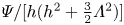 $\varPsi /[h(h^2+\frac 32\varLambda ^2)]$ plotted against scaled maximum gap
  $h/{R_{B}}$ (red and blue, respectively) for
  $\varLambda = \beta +\gamma h$ with
  $\beta =10^{-4}{R_{B}}$ and
  $\gamma =0.9$. With these parameter settings,
  $A$ and
  $\varPsi$ are functions only of
  $h/{R_{B}}$. Three sample solutions for
  $\psi$ are displayed by the density plots, corresponding to the values of
  $h/{R_{B}}$ indicated by the stars. The dashed line shows the corresponding result for the flux for the axisymmetric mode of figure 2(b), for which
  $\varLambda =0$.
For the axisymmetric mode, with  $\beta =\gamma =0$, the first term on the right-hand side of (2.28) reduces to
  $(h^3 P_x)_x$. Similarly, in the case of the lugworm-like mode (with
  $\beta \ll 1$ and
  $\gamma \approx 1$), we find a reduction to
  $\frac {5}{2}(h^3 P_x)_x$. These two versions of the model have no essential differences, as the differing factor of
  $\frac 52$ can be removed by a simple rescaling of the parameters
  $(\kappa,A,S)$. In the next section and beyond, we therefore set
 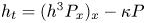 $h_t = (h^3P_x)_x-\kappa P$. In either case,
  $h(x,t)$ corresponds to the maximum size of the gap (in radius) at each axial position
  $x$.
$x$.
3. Pumping without leakage
Without any leakage into the porous wall ( $\kappa =0$), the model equations for the maximum gap
  $h(x,t)$ and conduit pressure
  $P(x,t)$ become
 $$\begin{gather} h_t ={-}q_x = (h^3 P_x )_x , \end{gather}$$
 $$\begin{gather}P = A f(x,\xi) + S (h-1), \end{gather}$$
where  $q(x,t)$ is the pumped flux in the (stationary) frame of the lugworm. We adopt the inlet and initial conditions,
 \begin{equation} P(0,t)=0 \quad \mbox{and} \quad h(0,t)=h(x,0)=1 ,\end{equation}
along with a forcing such that
 \begin{equation} f(x,\xi) = a(x)\sin\xi, \quad \xi=x-t, \quad a(x) = 1 - {\rm e}^{{-}x^2} - {\rm e}^{-(\ell-x)^2}. \end{equation}
The envelope  $a(x)$ suppresses wave motion at the ends of the conduit but leaves a uniform amplitude elsewhere (as noted by Wells (Reference Wells1945), the segments at the head and tail of a lugworm do not participate in peristalsis). The forcing function is illustrated in figure 4 for
  $\ell =6{\rm \pi}$. Provided the fluid pressure
  $P$ remains small in (3.2), this forcing generates between two and three peristaltic waves with the same shape as
  $f(x,\xi )$. The model has three key dimensionless parameters: the forcing strength
  $A$, stiffness
  $S$ and the conduit length
  $\ell$. Leakage, as considered in § 4, adds a fourth parameter
  $\kappa$.

Figure 4. Snapshots (blue) and envelope (red) for the model forcing function  $f(x,\xi )$ in (3.4) with dimensionless conduit length
  $\ell =6{\rm \pi}$.
3.1. Sample numerical solutions for open and closed conduits
Except at the ends of the conduit, the forcing is almost sinusoidal, implying that a regular train of propagating waves of peristalsis would be generated in the manner of figure 4 in the absence of any back reaction from fluid flow. However, depending on the conditions at the ends,  $x=0$ and
  $x=\ell$, large-scale pressure gradients may build up to limit transport. When the ends are open, with
  $P(0,t)=P(\ell,t)=0$ or
  $h(0,t)=h(\ell,t)=1$, such gradients are not expected and transport takes the form of a pulsing flux. But when the end at
  $x=\ell$ is closed (
 $q(\ell,t)=0$), pressure gradients must build up to terminate any transport over long times, once the peristaltic action has driven fluid into the conduit from the open end at
  $x=0$ and inflated it.
These scenarios are illustrated in figure 5 for two solutions (one with  $h(\ell,t)=1$, the other with
  $q(\ell,t)=0$) with moderate forcing amplitude and stiffness (
 $A=S=1$) and for a conduit length of
  $\ell =6{\rm \pi}$. The figure demonstrates how both solutions converge to temporally periodic states in which peristaltic waves grow from the left end, then reach a roughly constant amplitude whilst propagating steadily to the right, and finally disappear on colliding with the right end of the conduit. Also plotted are the averages over the final cycle of the peristaltic waves,
  $\langle h \rangle$ and
  $\langle P \rangle$, where
 \begin{equation} \langle G(x,t) \rangle = (2{\rm \pi})^{{-}1}\int_{t-{\rm \pi}}^{t+{\rm \pi}} G(x,\hat{t}) \, {\rm d} \hat{t} , \end{equation}
the time series of the mean conduit thickness,
 \begin{equation} {\bar{h}(t)} = \ell^{{-}1} \int_0^\ell h(x,t) \, {\rm d}\kern0.7pt x, \end{equation}
and the flux at the left end,  $q(0,t)$, together with its running average,
  $\langle q(0,t)\rangle$.

Figure 5. Snapshots of numerical solutions for (a,d) conduit thickness  $h(x,t)$ and (b,d) pressure
  $P(x,t)$ at a succession of times during the final cycle (spaced by
  $0.1{\rm \pi}$), for
  $\ell =6{\rm \pi}$, and the amplitude and stiffness parameters
  $A=S=1$. Panels (c,f) show corresponding time series of the change to the mean conduit thickness
  ${\bar {h}(t)}-1$ (blue) and the flux at the left end
  $q(0,t)$ (red); the dashed red line shows the running average of lefthand flux over a wave period,
  $\langle q(0,t) \rangle$. For (a–c), the conduit has impermeable walls and an open end (
 $P(\ell,t)=h(\ell,t)-1=0$); in (d–f) the right-hand end is closed (
 $q(\ell,t)=0$). The dashed blue lines in (a,b) and (d,e) show time averages,
  $\langle h(x,t) \rangle$ and
  $\langle P(x,t) \rangle$ over the final cycle. The insets to the right of (c,f) display
  $h(x,t)$ as a density on the
  $(x,t)$ plane for
  $t<80$ and
  $t<160$ (respectively).
When the conduit has an open right-hand end, a steady flux is maintained through the conduit in the final, temporally periodic state. As indicated by the plots of the mean thickness, however, peristalsis can lead to a net constriction of the conduit (with  $\langle h \rangle >1$), which reduces that flux in comparison to the spatially periodic version of the problem (considered in Appendix A). For the closed right-hand end, the outcome of peristalsis is the build up of a net pressure rise that opposes pumping and switches off any net transport. In the model, the form of the force law ensures that the pressure rise at the closed end is associated with unrestricted inflation, which is unlikely to be biologically relevant and could be avoided by a suitable modification to (3.2).
3.2. The limit of fixed displacement
In the limit  $A\gg 1$ with
  $S/A=O(1)$, the force balance on the wall (3.2) reduces to
 \begin{equation} h \approx 1 - \alpha a(x) \sin \xi , \quad \alpha = \frac{A}{S}.\end{equation}
If we ignore the modulation of the peristaltic waves in  $h$ due to the envelope
  $a(x)$ at the ends of the conduit, we may set
  $h_t\approx -h_\xi$ and then solve (3.1) for the pressure gradient:
 \begin{equation} P_x = \frac{1 - Q(t)}{h^3} - \frac{1}{h^2} .\end{equation}
Here,  $Q(t)$ denotes the flux in the frame of the peristaltic waves, which can be found by integrating (3.8) over the conduit and introducing the end pressures,
  $P(0,t)=0$ and
  $P(\ell,t) = P_{R}$, in the instance that
  $P_{R}$ is known. Alternatively, if there is a net pressure drop of
  $2{\rm \pi} \varGamma$ across each wave then
 \begin{equation} Q = \frac{3\alpha^2}{2+\alpha^2} - \frac{2\varGamma(1-\alpha^2)^{5/2}}{2+\alpha^2} ,\end{equation}
if we set  $a=1$ and
  $h\approx 1 - \alpha \sin \xi$ (cf. Shapiro et al. Reference Shapiro, Jaffrin and Weinberg1969).
In figure 6 the predictions of (3.7)–(3.9) with  $\varGamma =0$ and
  $a=1$ are compared against a numerical solution to the full problem with an open conduit (
 $P_{R}=0$),
  $\frac 32 S=A=10$ and
  $\ell =6{\rm \pi}$. Figure 6 also shows the corresponding solution with a closed end. In this case, the solutions converge initially to the predictions (3.7)–(3.9) with
  $\varGamma =0$. The solution then drifts as a large-scale pressure gradient builds up. With
  $Q=0$, (3.9) implies that a constant background gradient of
  $\varGamma ={3\alpha ^2}/[2(1-\alpha ^2)^{5/2}]\approx 3$ must build up, which is some way off the spatially varying mean gradient that is actually encountered in the numerical solution (see figure 6d). Similarly, the fixed displacement in (3.7) cannot capture the associated mean inflation of the conduit generated by the back pressure (figure 6c). Both shortcomings can be addressed by using the short-wavelength analysis presented in Appendix B (although the solutions in figure 6 do not possess sufficiently large
  $\ell$ to render that analysis quantitatively accurate; see figure 6d,e).

Figure 6. Numerical solutions for an impermeable conduit near the fixed-displacement limit with (a–c) an open end ( $P(\ell,t)=P_{R}=0$) and (d–f) a closed end (
 $q(\ell,t)=0$);
  $(A,S)=(10,15)$ and
  $\ell =6{\rm \pi}$. Shown are snapshots of (a,d)
  $h(x,t)$ and (b,e)
  $P(x,t)$ at the times
  $t=0.62+2{\rm \pi} j, j=0, 1, 2, \ldots$ (from red to blue), and (c,f) time series of the mean conduit thickness change
  ${\bar {h}}(t)-1$ (blue) and the instantaneous and cycle-averaged flux at the left end,
  $q(0,t)$ and
  $\langle q(0,t) \rangle$ (red solid and dashed). The dashed blue lines in (a,b) and (d,e) show averages,
  $\langle h\rangle$ and
  $\langle P\rangle$, for the final cycle. The black dashed lines in all panels show the predictions from (3.7) and (3.8). In (d,e) the dotted (green) line shows the results of the short-wavelength analysis of Appendix B. Insets to the right of (c,f) display
  $h(x,t)$ as densities on the
  $(x,t)$ plane for
  $t<100$.
3.3. Fixed displacement with near closure
The fixed-displacement solution makes sense only if  $\alpha <1$. Otherwise, the conduit is predicted to close at certain positions along the conduit and we cannot ignore the contribution of the pressure to (3.2). Sample numerical solutions corresponding to this situation for both an open and closed conduit are illustrated in figure 7. For the conduit with the open end, the solution rapidly converges to a quasi-steady train of localized peristaltic waves. Within each wave, the pressure is low and almost constant; in between them, the conduit becomes constricted and pressures become higher. The case of a conduit with a closed end is a little different, as discussed in more detail below, primarily because of the back pressure that builds up. Only at the beginning of the computation, before that back pressure is established, do isolated peristaltic waves appear.

Figure 7. Numerical solutions for an impermeable conduit with (a,b) an open end and (c,d) a closed end, for  $\ell =6{\rm \pi}$,
 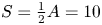 $S=\frac 12 A = 10$. Shown are (a,c) snapshots of
  $h(x,t)$ and (b,d)
  $P(x,t)/S$ at the times
  $t=1.26+2{\rm \pi} j, j=0, 1, 2, \ldots$ (from red to blue). In (e), time series of
  ${\bar {h}(t)}-1$ (blue),
  $q(0,t)$ (red solid) and
  $\langle q(0,t) \rangle$ (red dashed) are plotted for the solution in (c,d); that from (a,b) is plotted upto
  $t=29$ with thicker (black) dashed lines. The dashed blue lines in (a–d) show averages over the final cycle, and the (green) dots in (c) show (3.14). The insets display density plots of
  $h$ for the open (left) and closed (right) conduits.
Any near-closure of the conduit demands the revision of the analysis in § 3.2. In particular, although (3.7) and (3.8) remain relevant over the peristaltic waves (if there are no background pressure gradients), we must reinstate the pressure and take the limit  $h\ll 1$ to solve the problem over the constricted sections. Importantly, because flow is largely impeded over those constrictions,
  $Q\approx 1$. Away from the ends, the isolated peristaltic waves then have the solution,
 \begin{equation} h \sim 1 - \alpha \sin\xi \quad \textrm{and} \quad P_\xi \sim{-} (1 - \alpha \sin\xi)^{{-}2}. \end{equation}
On the other hand, the constrictions are described by
 \begin{equation} h = S^{{-}1/2} \eta(\xi), \quad P = S \varPi(\xi) \quad \text{and} \quad Q = 1 - S^{{-}1/2} \varUpsilon,\end{equation}
where
 \begin{equation} \varPi = \alpha \sin\xi - 1 \quad \text{and} \quad \alpha \eta^3 \cos\xi + \eta = \varUpsilon.\end{equation}
The solutions for the constrictions and isolated waves must be pieced together as described in Appendix C. One consequence of these matchings is the condition
 \begin{equation} \varUpsilon=2/[3\sqrt3(\alpha^2-1)^{1/4}] .\end{equation}
 The predictions in (3.10a,b)–(3.12a,b) are compared with numerical solutions of the full model for an open conduit with  $S=\frac 12 A=10$ and 100 in figure 8. The convergence to isolated waves and constrictions in the middle of the conduit is particularly clear in this example, with the various pieces of the profile matching well with the predictions in (3.10a,b)–(3.12a,b). Note that the constrictions substantially increase peak pressures during peristalsis, up to dimensional values of order
  $A\mathcal {P} \gg \mathcal {P}$. This feature indicates how one might resolve the discrepancy between the expected peristaltic pressure
  $\mathcal {P}=O(1)$ Pa and the range of experimental measurements for lugworms (
 $10^2$–
 $10^3$ Pa) listed in table 1: the conduit must nearly close during peristalsis for these organisms.

Figure 8. Further details of the solution from figure 7(a,b) (blue) and a similar solution, but closer to the fixed-displacement limit with  $S=\frac 12 A = 100$ (green). Shown are snapshots of (a)
  $h$ and (b)
  $\varPi =P/S$ at sixteen successive times during the final cycle (spaced by
  $0.1{\rm \pi}$), plotted against the travelling wave coordinate
  $\xi =x-t$. Magnifications of
  $h$ over a constriction and
  $P$ over an isolated peristaltic wave are shown in (c) and (d). The dashed lines show the predictions from (3.10a,b)–(3.12a,b).
In the case of the conduit with a closed end shown in figure 7(c,d), the increasing back pressure causes an inflation of the right end of the conduit. This inflation slowly ‘peels’ the constrictions off the impermeable wall, leaving a state with
 \begin{equation} h \sim \langle h \rangle - \alpha a(x) \sin \xi.\end{equation}
A single constriction remains over part of the wave cycle at the left end of the conduit when the forcing initiates a local collapse; otherwise the conduit remains open.
3.4. Pump characteristics
Steady-state fluxes predicted for peristaltic pumping with an open end ( $P_R=0$) are shown in figure 9 as a function of forcing amplitude
  $A$ for several values of
  $\alpha =A/S$. In the non-dimensionalization of the model, the two parameters
  $A$ and
  $S$ result from scaling the characteristic imposed force and body stiffness by the pressure measure
  $\mathcal {P}$. Their ratio,
  $\alpha$, is independent of
  $\mathcal {P}$ and, therefore, the wave speed
  $c$, representing a parameter that reflects the force exerted by the wall, the stiffness and geometry. Varying
  $A$ at fixed
  $\alpha$ can therefore be interpreted as varying the wave speed, holding fixed those quantities. Also shown in figure 9 are corresponding results for the perfectly spatially periodic version of the problem discussed further in Appendix A (for which calculations are more straightforward). In line with § 3.2, the flux becomes independent of
  $A$ for sufficiently high values owing to the convergence to the fixed-displacement problem. The results for the large values of
  $\alpha$ are also then similar to those for spatially periodic peristaltic waves. For lower values of
  $\alpha$, discrepancies arise mostly due to the mean constriction or inflation of the conduit.

Figure 9. Mean steady-state fluxes  $\langle q\rangle$ for (a) an open conduit and (b) spatially periodic peristaltic waves (Appendix A). The fluxes are plotted against
  $A$ for the values of
  $\alpha =A/S$ indicated. Also shown in (a) are the mean thickness of the conduit,
  $\langle \bar {h}\rangle$. In (b) the stars indicate the flux in the fixed displacement limit (3.9) for
  $\alpha <1$, and the dashed line shows the large
  $A$,
$A$,  $\alpha >1$ prediction in (3.11a–c) and (3.13).
It is common to express pump performance in terms of the ‘pump characteristic’: the relation between the mean flux and a net pressure drop applied along the conduit  $P_R$. Sample dimensionless pump characteristics, computed by imposing
  $P(\ell,t)=P_R$, are illustrated in figure 10 for
  $\alpha =\frac 23$ and in figure 11 for
  $\alpha =2$, with several values for
  $A$ and
  $\ell =6{\rm \pi}$. Nearer the fixed-displacement limit for
  $\alpha <1$, the relation between the net flux and pressure drop is linear, as expected from (3.9), but this relation becomes nonlinear as the conduit becomes constricted for lower
  $A$ or
  $\alpha >1$. In particular, as illustrated by the sample snapshots in figure 11(c), when the conduit becomes occluded, the peristaltic waves become shielded from the back pressure by any downstream constrictions. Only when the back pressure becomes sufficient to fully inflate the conduit and peel away all the constrictions does the flux become modified. This shielding effect is absent in the spatially periodic version of the problem (for which each peristaltic wave is forced to be identical), although the relation between the net flux and pressure drop also becomes nonlinear for constricted conduits (figure 11b).

Figure 10. (a) Mean fluxes and conduit thicknesses as a function of back pressure  $P(\ell,t)=P_R$ for
  $\alpha =\frac {2}{3}$ with
  $A=1$, 2, 4, 8, 16, 64 and 256 (from red to blue);
  $\ell =6{\rm \pi}$. The dashed line shows the flux in the fixed-displacement limit, computed directly from (3.8). In (b) we plot the corresponding fluxes for spatially periodic peristaltic waves subject to an adverse pressure gradient
  $\varGamma$ (see Appendix A); the dashed line indicates the prediction in (3.9). Panel (c) shows final snapshots (solid) and cycle average means (dashed) of
  $h$ and
  $P$, at the back pressures
  $S_R$ indicated by the stars in (a).

Figure 11. (a) Pump characteristics (mean conduit thickness  $\langle \bar {h}\rangle$ and flux
  $\langle q(0,t) \rangle$) against back pressure
  $P(\ell,t)=P_R$ for
  $A=2$, 4, 8, 20, 200 (from red to blue);
  $(\alpha,\ell )=(2,6{\rm \pi} )$. Corresponding fluxes for the spatially periodic problem are shown in (b). Panel (c) shows final snapshots (solid) and cycle average means (dashed) of
  $h$ and
  $P$, at the back pressures
  $S_R$ indicated by the stars in (a,b). The dotted lines show
  $h=1-\alpha \sin \xi$,
  $h=1-\alpha \sin \xi +P_R/S$ and
  $P=\alpha \sin \xi -1$.
If a peristaltic wave is not shielded from the back pressure by a downstream constriction, the wall displacement there is again described by (3.10a,b); see figure 11(c). Once those constrictions are peeled off, however, the conduit profile is modified to  $h\sim 1-\alpha \sin \xi + S^{-1} P_R$. The back pressure therefore must begin to peel the lugworm off the constrictions when
  $P_R>S$, as observed in figure 11(a).
Riisgård et al. (Reference Riisgård, Berntsen and Tarp1996) report measurement of the fluxes generated by lugworms enclosed in tight glass tubes, indicating that the flux is mostly a linear function of the frequency of the peristaltic waves. Assuming that wavelengths and amplitudes are fixed, the frequency corresponds to wave speed. Moreover, in the fixed-displacement regime, the dimensional flux per unit width  $c \mathcal {D} \langle q \rangle$ depends linearly on wave speed, suggesting that the lugworm is operating as a fixed-displacement pump. Riisgård et al. also suggest that conduits become constricted by peristalsis and the degree of backflow is limited. Thus, the lugworm pump may operate in a limit like that shown in figure 11.
Riisgård et al. (Reference Riisgård, Berntsen and Tarp1996) introduce hydrostatic back pressures to limit the peristaltic flux and empirically record the pump characteristic, observing that transport is eliminated for pressure drops of order 2 kPa; see figure 12(a). Other studies have suggested that lugworm peristalsis is associated with pressures of  $O(10^2)$ Pa (see table 1). But, in our model, the pressure scale,
  $12\mu c \mathcal {L} / \mathcal {D}^2 = O(1)$ Pa, is relatively small, and figure 10 implies that the introduction of an order-one dimensionless back pressure,
  $P(\ell,t)=P_R$, is usually sufficient to arrest pumping. Only if the conduit becomes significantly constricted at high forcing amplitude
  $A$ and stiffness
  $S$ (the limit taken in § 3.3) can dimensionless peristaltic pressures rise sufficiently to rationalize these observations (figure 11a).

Figure 12. (a) Experimental measurements of flux and back pressure for three lugworms, as presented by Riisgård et al. (Reference Riisgård, Berntsen and Tarp1996). Pumping frequency is indicated by the colour and symbol (see the legend). In (b) the data for frequencies of 5, 6 and 7 cycles/minute (i.e. the redder triangles) are scaled in the manner of our theoretical model (adjusting  $c=0.04f$ m s
 $^{-1}$ according to frequency
  $f$ cycles/s).
The measurements of Riisgård et al. (Reference Riisgård, Berntsen and Tarp1996) are replotted in figure 12(b), scaling the data as in the theoretical model. However, a Riisgård et al. also note that adding back pressure reduces wave frequency and thereby the flux, suggesting an adaptive peristaltic action. To partly account for this effect, only the measurements with higher frequency (5–7 cycles/minute) are replotted in figure 12(b). This replotted data does suggest a relatively flat pump characteristic, as seen in figure 11(a) for  $P_{R}< S$.
4. Leaky pumping
4.1. Permeable burrows
Now we add a leakage through the burrow wall into the (non-deforming) porous half-space beyond ( $\kappa \ne 0$), but otherwise consider the same problem as above for a conduit with a closed end (
 $q(\ell,t)=0$). The system to solve is
 $$\begin{gather} h_t = (h^3 P_x )_x - \kappa P, \end{gather}$$
 $$\begin{gather}P = A a(x) \sin \xi + S (h-1) , \end{gather}$$
which implies that, in any temporally periodic state,
 \begin{equation} \langle q(0,t) \rangle = \kappa \int_0^\ell \langle P(x,t) \rangle \,{\rm d}\kern0.7pt x .\end{equation}
 Sample numerical solutions, corresponding to those in figures 5(d–f) and 6(d–f), but with  $\kappa >0$, are shown in figure 13. Again, the peristaltic waves pump fluid into the conduit. This time, however, due to a net leakage of water through the burrow wall, the pressure gradient no longer builds up to the same degree. The deformation of the pumper's surface and the inflation of the conduit are thereby reduced, and a finite flux at the left end in the steady state is maintained over long times. Also, because of the spatially oscillating pressure of each peristaltic wave, water can be drawn back out of the porous wall during the times that the pressure reaches its minima, offsetting the leakage occurring during the pressure maxima. This short circuit by the leakage is illustrated by the snapshots and cycle averages of
  $P(x,t)$, which sets the degree of drainage through
  $-\kappa P$ in (4.1). As a result, the net flux into the porous wall is partly suppressed. In the final steady state, the net flux increases towards the right end of the conduit where pressures are highest, but there is a net drainage from the half-space into the conduit over the first wavelength (see the final cycle average of
  $P$ in figure 13b).

Figure 13. Solutions for a leaky conduit with  $\kappa =0.0333$ and a closed end (
 $q(\ell,t)=0$), for (a–c)
  $(A,S)=(1,1)$ and (d–f)
  $(A,S)=(10,15)$;
  $\ell =6{\rm \pi}$. Shown are final snapshots (dashed) and cycle averages (solid) of (a,d)
  $h(x,t)$ and (b,e)
  $P(x,t)$, and (c,f) time series of
  ${\bar {h}(t)}-1$ (blue),
  $q(0,t)$ and
  $\langle q(0,t) \rangle$ (red solid and dashed). The (green) dotted lines in (d–f) show the short-wavelength predictions of Appendix B. The insets to the right of (c,f) show
  $h(x,t)$ as densities on the
  $(x,t)$ plane (for
  $t<80$).
Increasing the permeability parameter  $\kappa$ reduces the inflation and pressure gradient still further, as illustrated in figure 14. For small
  $\kappa$, the net flux through the left end of the conduit can be determined by substituting the pressure solution
  $P=P_{0}(x,t)$ for
  $\kappa =0$ into the constraint (4.3), to give the linear prediction
 \begin{equation} \langle q(0,t) \rangle = \kappa \int_0^\ell\langle P_{0} \rangle \, {\rm d}\kern0.7pt x ,\end{equation}
which is also shown in figure 14. However, the most interesting feature of the suite of computations shown in this figure is how the net leftward flux first increases as  $\kappa$ is first raised above zero, but then reaches a maximum and finally declines once the short circuit through the porous medium exacts its toll. Consequently, there is a distinguished value of
  $\kappa$ for which the transport through the burrow is maximized.

Figure 14. Final cycle averages (solid) of (a,c)  $h(x,t)$ and (b,d)
  $P(x,t)$ for four values of
  $\kappa$ (increasing from blue to red), with (a,b)
  $(A,S)=(1,1)$ and (c,d)
  $(A,S)=(10,15)$;
  $\ell =6{\rm \pi}$. The final snapshots are also plotted (dashed) for the solutions with the smallest value of
  $\kappa$. In panel (e) we show the final, cycle-averaged values of the flux at
  $x=0$ against
  $\kappa$ for a larger set of computations. The values of
  $\kappa$ for the solutions shown in (a–d) are indicated by stars and circles. The dashed lines show the approximation in (4.4). The dotted lines in (c), (d) and (e) show the short-wavelength predictions of Appendix B.
Solutions at higher forcing amplitude,  $S=\frac 12 A=10$, are shown in figure 15. These parameter settings match those for the solutions with an impermeable wall in figure 7, for which isolated peristaltic waves separated by constrictions appear before back pressures force the conduit to remain open along its length. In figure 15 the back pressures become limited for increasing leakage, and some of the constrictions are then no longer peeled away from the wall. In fact, because the leakage term
  $-\kappa P$ in (4.1) does not vanish when
  $h\to 0$ (unlike the flux), the integration of (4.1) can permit
  $h$ to become unphysically negative during pumping. Such closures do indeed arise over the constrictions for the largest values of
  $\kappa$ in figure 15. To avoid unphysical solutions with
  $h<0$, one can add a switch on the right-hand side of (4.1) that sets
  $h_t=0$ if both
  $h\leq 0$ and
  $(h^3P_x)_x-\kappa P <0$. This switch prevents
  $h$ from becoming negative and instead holds the conduit at zero thickness (at least to within numerical errors), whilst allowing the worm surface to become pulled back off the porous wall from an existing closure if forced to do so. The solutions shown in figure 15 with higher
  $\kappa$ incorporate the switch. However, these solutions cannot maintain the constraint in (4.3), and the pressure solution from (4.2) has no meaning if
  $h\leq 0$ (the contact force being omitted from this relation), obscuring how fluid must flow in the porous medium (§ 2.2.2). Overall, although we may avoid negative conduit thicknesses by adding the switch to (4.1), the physical significance of these solutions is not clear and they must be viewed with some caution.

Figure 15. (a) Final snapshots of  $h(x,t)$ and
  $P(x,t)$ for larger-amplitude numerical solutions with
  $\kappa =0$ and
  $\kappa >0$ (with
  $\kappa$ increasing from blue to red), for
  $A=20$,
  $S=10$ and
  $\ell =6{\rm \pi}$. The dot-dashed line shows
  $A\sin \xi -S$, and the pressure is not plotted where
  $h\leq 0$. Density plots of
  $h(x,t)$ for the five solutions are displayed in (b) (for
  $t<80$). Panel (c) shows the final net lefthand flux
  $\langle q(0,t)\rangle$ against
  $\kappa$ for a larger suite of computations. The stars indicate the values of
  $\kappa$ for the solutions shown in (a), the dashed line shows the approximation in (4.4), and over the shaded region the conduit closes during peristalsis.
The parameter  $\kappa$ was estimated earlier to be
  $O(10^{-2})$ for typical lugworm conditions. One might therefore conclude from figures 14(e) and 15(c) that the lugworm may pump optimally for transport. However, the lugworm burrow is armoured by mucus to make it less permeable over the gallery, and the burrow usually continues beyond the head into a feeding pocket. This leads us to consider a different problem in which the burrow wall is impermeable, but fluid is pumped into a leaky headspace beyond.
4.2. Pumping into a feeding pocket
In the ‘normal cyclical pattern’ proposed by Wells (Reference Wells1945, Reference Wells1966) the wall of the gallery is impermeable and all the fluid escapes through a cylindrical head shaft. More recently, it has been suggested that water escapes from the feeding pocket in a more distributed fashion (Meysman et al. Reference Meysman, Galaktionov and Middelburg2005; Wethey et al. Reference Wethey, Woodin, Volkenborn and Reise2008; Delefosse et al. Reference Delefosse, Kristensen, Crunelle, Braad, Dam, Thisgaard, Thomassen and Høilund-Carlsen2015), although the motivating observations have not always been in situ. Indeed, Wells and other studies (e.g. Hüttel Reference Hüttel1990; Volkenborn et al. Reference Volkenborn, Polerecky, Wethey and Woodin2010) offer persuasive evidence to suggest that a significant fraction of the water leaves through the head shaft.
When all the water is lost through a cylindrical head shaft, a one-dimensional version of Darcy's law applies, setting the flux,
 \begin{equation} c A_p q = \frac{K (p_{R}-p_{B}) A_h}{\mu h_B}, \end{equation}
as exploited by Riisgård et al. (Reference Riisgård, Berntsen and Tarp1996), where  $h_{B}$ and
  $p_{R}$ denote the depth and pressure of the feeding pocket, and
  $A_h$ is the effective area of cross-section of the head shaft. Scaling as before, we find the dimensionless boundary condition,
 \begin{equation} p(\ell,t) = P_{R} = \lambda q(\ell,t) , \quad \lambda = \frac{h_{B} \mathcal{D}^2 A_p }{12 \mathcal{L} A_h K }, \end{equation}
where  $A_p$ is the cross-sectional area of the conduit. This condition, which can be applied on numerical solutions to (3.1) and (3.2) at the right of the conduit, corresponds to the selection of the ‘operating point’ for lugworms employed by Foster-Smith (Reference Foster-Smith1978) and Riisgård et al. (Reference Riisgård, Berntsen and Tarp1996). Adopting an area for the head shaft of
  $A_h =3$ cm
 $^2$ (a radius of about a centimetre) and taking
  $h_{B}=20$ cm and
  $K=5.5\times 10^{-11}$ m
 $^2$, leads to the parameter estimate,
  $\lambda =O(10^3)$. Nevertheless, this permeability assumes that the head shaft has the same resistance to flow as the surrounding sediment, in conflict with the implied channelization along it. If the sand in the head shaft is loosened by the worm, then fluidized by flow, as described by Wells (Reference Wells1945), then
  $K$ must be orders of magnitude larger, rendering
  $\lambda$ correspondingly smaller. Indeed, if smaller particles become carried away by the current, in the manner of the piping failure of dams,
  $\lambda$ may be smaller still. If we revise the value of the permeability within the head shaft to
  $K=10^{-9}\ {\rm m}^2$ (a value typical for loose sand), then we arrive at the estimate,
  $\lambda \approx 28$.
Alternatively, for an opposite extreme, we assume that the porous medium is homogenous and fluid escapes uniformly from a spherical feeding pocket of radius  $\mathcal {R}_{\mathcal {B}}$ in the manner of a point source. Ignoring the burrow, the pressure surrounding the pocket is then, on adding an image to account for the boundary condition
  $\tilde {p}=p_{B}-\rho g h_{B}$ at
  $\tilde {z}=h_{B}$,
 \begin{equation} \tilde{p}(\tilde{r},\tilde{z},\tilde{t}) = p_{B} - \rho g \tilde{z} + \mathcal{R}_{\mathcal{B}} (p_{R} - p_{B}) \left[ \frac{1}{ \sqrt{\tilde{r}^2 + \tilde{z}^2} } - \frac{1}{ \sqrt{\tilde{r}^2 + (2h_{B}-\tilde{z})^2} } \right], \end{equation}
where  $\tilde r$ is a (cylindrical-polar) radial coordinate centred at the feeding pocket. The dimensionless flux through the seafloor (the sediment–water interface) at
  $\tilde {z}=h_{B}$ is
 \begin{equation} - \frac{2{\rm \pi} K}{\mu c A_p} \int_0^\infty [\tilde{p}_{\tilde{z}}(\tilde{r},h_{B},\tilde{t}) + \rho g] \tilde{r}\, {\rm d} \tilde{r} = \frac{4{\rm \pi} K \mathcal{R}_{\mathcal{B}}}{\mu c A_p} (p_{R} - p_{B}) = \frac{12{\rm \pi} K \mathcal{L} \mathcal{R}_{\mathcal{B}}}{A_p \mathcal{D}^2} P_{R}, \end{equation}
which must match  $q(\ell,t)$. Thus, we again arrive at the boundary condition in (4.6), but this time with parameter
 \begin{equation} \lambda = \frac{A_p \mathcal{D}^2}{12 {\rm \pi}K \mathcal{L} \mathcal{R}_{\mathcal{B}}}, \end{equation}
which can be estimated to be about  $32$ if
  $K=5.5\times 10^{-11}\ {\rm m}^2$.
Either way, we may compute solutions to (3.1) and (3.2) with the revised right-hand boundary condition in (4.6), taking  $\lambda$ to be an order-one parameter. For
  $\lambda \to 0$, (4.6) enforces the zero-pressure condition
  $P(\ell,t)=P_{R}=0$ and the solutions approach those for an open end, whereas no flux is implied for
  $\lambda \to \infty$, as for a closed end; parameter settings in between bridge across these limits. Results for the final mean conduit thickness
  ${\bar {h}(t)}$, right-hand average pressure
  $\langle P(\ell,t)\rangle$ and flux
  $\langle q \rangle$ are displayed in figure 16.

Figure 16. (a,c) Average righthand pressures  $\langle P_{R} \rangle$, and (b,d)
  $\langle q \rangle$ and
  $\langle {\bar {h}(t)}\rangle -1$ against leakage parameter
  $\lambda$ for solutions to (3.1) and (3.2) with the boundary condition in (4.6) (stars). Solutions with
  $(A,S)=(16,24)$ (
 $\alpha =\frac 23$) are shown in (a,b), and for
  $(A,S)=(16,8)$ (
 $\alpha =2$) are shown in (c,d);
  $\ell =6{\rm \pi}$. The dashed and dot-dashed lines show the limits derived using the solutions for open (
 $P_{R} \sim \lambda \langle q\rangle$) and closed (
 $\langle q\rangle \sim \langle P_{R}\rangle /\lambda$) conduits, respectively. The solid lines translate data from computations with the boundary condition
  $P(\ell,t)=P_{R}$, taking
  $\lambda =P_{R}/\langle q \rangle$.
Solutions computed with the boundary condition in (4.6) differ from those employing the right-hand pressure condition  $P(\ell,t)=P_{R}$, as used earlier in § 3.4, primarily near the right-hand end of the conduit. However, once one arrives at the final, temporally periodic state, this former condition implies that
  $\langle P(\ell,t) \rangle = \lambda \langle q(\ell,t) \rangle$. Thus, if one reinterprets
  $\lambda$ as
  $P_{R}/\langle q(\ell,t) \rangle$, one can translate data from solutions with
  $P(\ell,t)=P_{R}$ to the feeding-pocket problem. This translation is illustrated in figure 16, where data from solutions with fixed right-hand pressure are added to the plots. In other words, the pump characteristics discussed in § 3.4 remain relevant with (4.6).
For the fixed-displacement cases in figure 16(a,b), the transition between the limits of open and closed conduits is relatively gradual, taking place when  $\lambda$ is of
  $O(10)$. If there are constrictions (figure 16c,d), the passage away from the open-conduit limit takes place abruptly when
  $\lambda >15$ (for the parameter settings shown). This abrupt change results from the constrictions that again shield pumping from the downstream boundary condition. Our estimates for the magnitude of
  $\lambda$ based on typical conditions for the lugworm environment suggest that pumping would occur over that transition.
5. Discussion
At low Reynolds number, long-wave peristaltic pumping corresponds to a lubrication problem in which a forced, flexible wall cyclically drives fluid down a conduit. Sections of the conduit may collapse over part of the wave cycle for sufficiently strong forcing, leading to isolated peristaltic waves transporting fluid close to the wave speed. In this paper we provided an analysis of this situation, capturing consistently any near-closures of the conduit by coupling lubrication theory for the fluid with a law encompassing the force balance on the flexible wall. The coupled model captures the limit in which the wall displacement becomes fixed, except where any constrictions arise, and can be used to predict ‘pump characteristics’ (the relation between flux and net pressure drop).
Motivated by peristaltic pumping of marine worms, we considered pumping down a conduit with the form of a narrow annular gap. We also included the leakage of fluid through the outer wall into a surrounding porous medium, using slender-body theory to solve the associated Darcy problem. In this situation, when the wall is impermeable and the downstream end of the conduit is closed, an adverse back pressure is set up to prevent any net flux. If the wall is permeable, however, the back pressure is relieved, allowing transport. But for very leaky walls, the flow through the porous medium short circuits that in the conduit, again eliminating any net flux. Maximum transport therefore arises at an optimal rate of leakage. Some marine worms use mucus to armour the wall of their burrows, rendering them less permeable, and instead pump water into a feeding pocket or head shaft at the end of the burrow. A variation of the model accounts for this alternative situation by employing a boundary condition at the burrow's end that permits leakage there.
For fixed-displacement peristaltic waves, lubrication theory predicts pumping pressures that are dictated by the fluid viscosity, the pump wavelength and speed, and the conduit thickness (Shapiro et al. Reference Shapiro, Jaffrin and Weinberg1969). Measurements for lugworms in glass tubes (Riisgård et al. Reference Riisgård, Berntsen and Tarp1996), however, suggest pumping pressures that are two orders of magnitude higher. This discrepancy can only be explained by arguing that the conduit nearly closes during peristalsis. Pressures can then be achieved that are much greater than the expected lubrication pressure ( $\mathcal {P}$ in our analysis). In other words, these pumpers must operate close to a fixed-displacement limit with constrictions. Armed with that insight, the pump characteristics observed for lugworms can be plausibly reproduced by the model. However, the model cannot account for the change in pump frequency with net pressure drop also noted experimentally (which suggests that peristalsis adapts to ambient conditions). Our exploration of the effect of leakage, either through the burrow wall or from a head shaft or feeding pocket, confirms that the loss of water into the surrounding porous sediment is significant, as demanded by the inferred bioturbative action of marine worms on their environment.
All that said, our model is idealized and several improvements are needed for any connection to an application. For example, closer comparison of the model with observations of lugworm activity requires stronger constraints on pumped waveforms; we activated peristalsis here by applying a sinusoidal force to the worm's surface, assuming that its cross-section remains circular. However, detailed reports of the shape of the lugworm's peristaltic waves are lacking in the literature: in some cases, the lugworm is portrayed as residing along the bottom of the burrow, sending waves along its upper surface (e.g. Wells Reference Wells1966; Toulmond & Dejours Reference Toulmond and Dejours1994; Riisgård et al. Reference Riisgård, Berntsen and Tarp1996); other illustrations picture a centrally located position with more symmetrical waves (Just Reference Just1924; Krüger Reference Krüger1971; Delefosse et al. Reference Delefosse, Kristensen, Crunelle, Braad, Dam, Thisgaard, Thomassen and Høilund-Carlsen2015). Were observations available for realistic wave shapes, then one might attempt an inverse problem to establish the forcing activating peristalsis. Alternatively, one might consider optimization problems to determine the best wave shape, given certain objectives (cf. Walker & Shelley Reference Walker and Shelley2010).
Our use of the leading-order slender-body theory to account for the leakage through the burrow wall also has its limitations (Handelsman & Keller Reference Handelsman and Keller1967; Hinch Reference Hinch1991), with better approximations rendering leakage dependent non-locally on conduit pressure. These refinements could also be used to account for the geometry of a curved burrow centreline, a varying permeability of the burrow wall (mucus armouring) and the overlying sediment–water interface, without necessarily solving a three-dimensional Darcy flow problem (cf. Meysman et al. Reference Meysman, Galaktionov and Middelburg2005). Another major simplification that we adopted was to assume that the sediment does not deform under peristalsis. When the burrow wall is armoured with mucus, this is perhaps a fair approximation (Wells Reference Wells1945 and others report how the gallery wall can become exposed and stand up against gravity when water levels recede; if the exposed length of burrow wall is several centimetres, as needed to make the feature noteworthy, this implies a yield stress exceeding  $10^3$ Pa, which is at the upper end of the pumping pressure range measured for lugworms, suggesting an armoured burrow wall will indeed not deform under peristalsis). But when the sediment is more loosely packed, lubrication pressures will compact that medium. A poro-elastic model (e.g. Detournay & Cheng Reference Detournay and Cheng1993) may then be more suitable, which complicates the leakage dynamics by adding the diffusion of the pore pressure. Lugworms certainly fluidize the head shaft through a combination of through flow and mechanical activity (Wells Reference Wells1945; Hüttel Reference Hüttel1990), raising the interesting question of what dictates the shape of that conical, more loosely packed feature.
Perhaps the most important biological aspect of peristaltic pumping through a sandy burrow is how lugworms and other organisms achieve bioturbation by flushing oxygenated water and nutrients through the surrounding sediment. Previous models of this process prescribe a burrow pressure to drive flow through the sediment (cf. Meysman et al. Reference Meysman, Galaktionov and Middelburg2005; Wethey et al. Reference Wethey, Woodin, Volkenborn and Reise2008). This pressure, however, follows from the detailed fluid dynamics of the pump, which is a key ingredient in our model. The spatially varying pressure field that develops during peristalsis can drive fluid out of a leaky conduit near the head and back into the burrow nearer the tail. Overall, the net recirculation is sensitive to the peristaltic dynamics, and can force flow through the sediment even if permeabilities are relatively small, or when there is minimal net transport down the burrow.
Acknowledgements
This work was initiated at the Geophysical Fluid Dynamics Summer Study Program, 2022, which is supported by the National Science Foundation.
Declaration of interest
The authors report no conflict of interest.
Appendix A. Periodic pumping with leakage
For the steadily propagating, purely periodic problem, after transforming into the frame of the forcing and expressing all variables in terms of  $\xi$, we have
 $$\begin{gather} (h^3 P_\xi)_\xi = \kappa P - h_\xi, \end{gather}$$
 $$\begin{gather}P = A \sin \xi + S (h-1) . \end{gather}$$
Note that, for any finite  $\kappa$, the spatial average of (A1) implies that
  $\langle P \rangle =0$, and so
  $\langle h\rangle =1$ from (A2). In other words, there can be no net constriction or inflation of the conduit. One can further add a constant adverse pressure gradient
  $\varGamma$ to (A1) (to give an additional term
  $-3\varGamma h^2 h_\xi$ on the left). This gradient suppresses the flux, eventually reversing the direction of net flow, as illustrated in figures 10 and 11 of the main text.
Without leakage ( $\kappa =0$), and in the limit
  $S\gg 1$ with
  $\alpha =A/S<1$, the displacement of the wall is fixed, and
 \begin{equation} h \sim 1 - \alpha \sin \xi \quad \text{and} \quad Q = \frac{3\alpha^2}{2+\alpha^2}, \end{equation}
as in Appendix B. For  $\alpha >1$, a constriction must form. In this case, the fluid largely collects into an isolated wave with constant pressure
  $P_b$ spanning periodic extensions of the interval
  $\frac {3}{2}{\rm \pi} -\chi < \xi <\frac {3}{2}{\rm \pi} +\chi$, where
 \begin{equation} h \sim 1 + \frac{P_b}{S} - \alpha \sin \xi, \quad P_b ={-}1-\alpha\cos\chi, \quad {\rm \pi}-\alpha\sin\chi+\alpha\chi\cos\chi = 0,\end{equation}
(given that  $\langle h \rangle =1$ and the constriction has
  $h\approx 0$). Pressure gradients become restricted to the constrictions intervening between the isolated waves, with
 \begin{equation} P \sim A\sin\xi-S.\end{equation}
Sample solutions for three pairs of values for  $(S,A)$ are shown in figure 17. As
  $\kappa$ is increased for fixed
  $(S,A)$, more water drains into the porous medium, reducing the pressure gradient and allowing the conduit to become more constricted. For sufficiently high
  $\kappa$, the short circuit introduced by the flow through the porous half-space eventually throttles the flux and
  $P$ becomes small, giving
  $h\sim 1-\alpha \sin \xi$, as illustrated in figure 17(a). This further implies that
 \begin{equation} P \sim{-}(\kappa S)^{{-}1}A\cos\xi \quad \text{and} \quad Q \equiv \langle h^3 P_\xi \rangle \to \tfrac{3}{8}\kappa^{{-}1}\alpha^2(4+\alpha^2).\end{equation}
Figure 17. Steadily propagating periodic solutions for (a)  $(S,A)=(1,1)$ (top) and
  $(S,A)=(15,10)$ (bottom), with
  $\kappa =0$ (dashed),
  $0.2$,
  $0.6$,
  $1.6$ and
  $4.8$. The black dots show
  $1-S^{-1}A\sin \xi$. The corresponding mean flux
  $\langle Q \rangle$ for a wider set of solutions is shown in (b); the dashed lines show the prediction in (A6a,b). Solutions with
  $(S,A)=(10,20)$ are plotted in (c) for
  $\kappa =(0,1,2,\ldots,6)\times 10^{-3}$; the inset shows a magnification of the constriction and the dots show the predictions in (A4a,b) and (A5).
At the highest amplitudes and leakages (figure 17c), the conduit again closes over the constrictions, terminating the branch of solutions computed from (A1) and (A2). The solutions for the narrow window of values of  $\kappa$ below this limit vary primarily over the constrictions, as illustrated in figure 17(c). Elsewhere, the solutions match up with the predictions from (A4a,b) and (A5).
Appendix B. Peristaltic waves along a slowly varying conduit
When  $\ell \gg 1$, the peristaltic waves have a relatively short wavelength and we may asymptotically reduce the model equations. Note that the analysis in this appendix can further be used to take account of any longer-scale variations in physical conditions along the length of the conduit, and could be applied to other problems of peristalsis.
For the impermeable conduit, we take  $(S,A)=O(\ell )$, and set
 \begin{equation} \varepsilon=\ell^{{-}1}, \quad X= \varepsilon x, \quad P = \varepsilon^{{-}1} \varPi(X) + {\hat{P}}(\xi,X) + \cdots, \quad h = \varTheta(X) + \hat{h}(\xi,X) + \cdots . \end{equation}
Here, we ignore the variation of  $a(x)$ near the ends and any ambiguity in the decompositions of
  $h$ and
  $P$ is removed by demanding that
  $\hat{h}(\xi,X)$ and
  ${\hat {P}}(\xi,X)$ have no net average over
  $\xi$. Equation (3.1) then becomes
 \begin{equation} -h_\xi ={-}q_\xi - \varepsilon q_X, \quad q ={-}(\varTheta+\hat{h})^3(\varPi_X+{\hat{P}}_\xi)+\cdots. \end{equation}
Averaging the first relation over  $\xi$ implies that
  $\mathcal {Q}_X=0$, where
  $\mathcal {Q}=\langle q \rangle$; i.e. the wave-cycle average of
  $q$ must be independent of
  $X$. To leading order in
  $\varepsilon$, and in combination with (3.2), we then find that
 \begin{equation} -\hat{h}_\xi = [ (\varTheta+\hat{h})^3 (\varPi_X + {\hat{P}}_\xi) ]_\xi, \quad \varPi = {\hat{S}} (\varTheta - 1) ,\quad \hat{h} ={-}\alpha a \sin\xi , \end{equation}
where  ${\hat {A}}=\varepsilon A$,
  ${\hat {S}}=\varepsilon S$ and
  $\alpha ={{\hat {A}}}/{{\hat {S}}}$. Integrating the first of these relations now gives
 \begin{equation} \mathcal{Q} ={-} \hat{h} - (\varTheta+\hat{h})^3 (\varPi_X + {\hat{P}}_\xi). \end{equation}
That is,
 \begin{equation} \varPi_X + {\hat{P}}_\xi = \frac{\varTheta-\mathcal{Q}}{(\varTheta-\alpha a\sin\xi)^3} - \frac{1}{(\varTheta-\alpha a\sin\xi)^2} , \end{equation}
and so averaging over  $\xi$ furnishes
 \begin{equation} \varPi_X = {\hat{S}} \varTheta_X = \frac{3\alpha^2a^2\varTheta-\mathcal{Q}(2\varTheta^2+\alpha^2a^2)} {2(\varTheta^2-\alpha^2a^2)^{5/2}}, \end{equation}
assuming that the envelope of the forcing  $a$ is a function of the longer-scale variable
  $X$.
$X$.
Equation (B6) can be integrated from  $(X,\varTheta )=(0,1)$ out to
  $X=1$, taking
  $\mathcal {Q}$ as a parameter. If
  $a=1$ and
  $\mathcal {Q}=3\alpha ^2/(2+\alpha ^2)$, the solution is
  $\varTheta =1$ and
  $\varPi =0$, corresponding to the conduit with an open left-hand end. For
  $\mathcal {Q}=0$ and the conduit with a closed right end, the integration of (B6) leads to the results included in figures 6(d,e) and 14(c–e), and shown further in figure 18 for solutions closer to the short-wavelength limit. The short-wavelength analysis successfully incorporates the back pressure resulting from the closed end and the resulting mean inflation of the conduit, but becomes inaccurate near the ends owing to the form of the envelope of the forcing
  $a(x)$ in (3.4) that is too short to be adequately captured by the long-scale variable
  $X$.
$X$.

Figure 18. Final snapshots (dashed) and cycle averages (solid) of (a)  $h(x,t)$ and (b)
  $P(x,t)$ for solutions with
  $\kappa =0$,
  $10^{-3}$,
  $\frac 14\times 10^{-2}$,
  $10^{-2}$ and
  $0.1$ (increasing from blue to red);
  $(A,S,\ell )=(10,15,20{\rm \pi} )$ and the right end of the conduit is closed. The dots show the predictions of the short-wavelength analysis.
With a leaky conduit, taking the same multiple-scale limit as before, but with  $\kappa =\varepsilon ^2{\hat {\kappa }}$, we develop (4.1) and (4.2) into
 $$\begin{gather} \hat{h}_\xi = q_\xi + \varepsilon q_X + \varepsilon {\hat{\kappa}} {\hat{S}}(\varTheta-1) + \cdots, \end{gather}$$
 $$\begin{gather}h = \varTheta - \alpha a \sin\xi + \cdots, \quad P = \frac{{\hat{S}}}{\varepsilon} (\varTheta - 1) + {\hat{P}} + \cdots. \end{gather}$$
Hence, taking the  $\xi$ average,
 \begin{equation} \mathcal{Q}_X ={-} {\hat{\kappa}} {\hat{S}} ( \varTheta-1 ),\end{equation}
where  $\mathcal {Q}(X)=\langle q \rangle$ as before. Repeating the analysis now couples (B6) to (B9). The solutions of this coupled system for
  $\varTheta (0)=1$ and
  $\mathcal {Q}(1)=0$ are included in figures 14 and 18.
Appendix C. Matching isolated peristaltic waves and constrictions
The solutions for the isolated peristaltic waves and constrictions of § 3.3 must be matched together over narrow regions of width  $S^{-1/2}$ surrounding the points,
  $\xi =\xi _*^\pm$, where
  $\alpha \sin \xi _*^\pm = 1$ (or
  $\alpha \cos \xi _*^\pm = \pm \sqrt {\alpha ^2-1}$). Setting
  $\xi =\xi _*+S^{-1/2}\zeta$ and
  $h = S^{-1/2}\varTheta (\zeta )$ over the matching layers, the leading-order solution there satisfies
 \begin{equation} \varTheta' \sim \frac{\varUpsilon - \varTheta}{\varTheta^3} - \alpha \cos\xi ,\end{equation}
with  $\xi =\xi _*^\pm$. This gives
 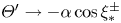 $\varTheta ' \to -\alpha \cos \xi _*^\pm$ and a match to the wider conduit for
  $\varTheta \gg 1$, and
  $\varUpsilon \to \varTheta + \alpha \varTheta ^3 \cos \xi _*^\pm$ to the other side, effecting a match with the constriction.
In fact, (C1) can be applied throughout the entire region containing the constriction and matching layers, provided  $\xi$ is interpreted as a slower spatial scale (in comparison to
  $\zeta$). To the left of the constriction, where this combined region begins,
  $\xi \approx \xi _*^-$ and the solution to (C1) captures the rapid thinning of the conduit from the isolated wave to the constriction, which corresponds to a stable fixed point satisfying
  $\varUpsilon \to \varTheta + \alpha \varTheta ^3 \cos \xi _*^-$. On progressing into the constriction, the solution to (C1) remains at the corresponding quasi-stationary fixed point as
  $\xi$ slowly varies. Eventually, the constriction terminates at
  $\xi =\xi _*^+$, where the fixed point disappears, prompting the rapid transition to the beginning of the next isolated wave. The disappearance of the stable fixed point demands that
  $\varTheta '=\varTheta ''=0$ for
  $\xi =\xi _*^+$, which furnishes (3.13). Note that this construction is different from that selecting the flux in Takagi & Balmforth (Reference Takagi and Balmforth2011b) (see also O'Brien & Gath Reference O'Brien and Gath1998; Ashmore et al. Reference Ashmore, Hosoi and Stone2003; Benilov et al. Reference Benilov, Benilov and Kopteva2008).


 Open access