


1 Introduction
Swept-wing crossflow-dominated boundary layers subject to low free-stream turbulence are well known to develop stationary streamwise-oriented crossflow vortices as a primary instability. Despite the small amplitude of the primary vortices, they result in a mean flow distortion giving rise to high-frequency secondary instabilities, which ultimately breakdown to turbulence, see Reed, Saric & Arnal (Reference Reed, Saric and Arnal1996), Saric, Reed & White (Reference Saric, Reed and White2003), White & Saric (Reference White and Saric2005) and Bonfigli & Kloker (Reference Bonfigli and Kloker2007). Detailed information on the secondary instabilities, specifically their amplification and spatial topology, is instrumental in understanding, and ultimately predicting, where laminar–turbulent transition will occur. The main effect of the primary stationary crossflow vortices on the laminar flow is to redistribute momentum across the boundary layer by advection about their vortical axes. Downwash and upwash events on the respective sides of the crossflow vortex result in a spanwise modulation of the, otherwise spanwise homogeneous, boundary layer in the form of a series of high- and low-speed regions. The resulting instantaneous and mean flow present elevated shear stress components in two spatial directions.
For engineering purposes, transition prediction is typically performed using the classical semi-empirical
 $\text{e}^{N}$
-method, where
$\text{e}^{N}$
-method, where
 $N$
indicates the natural logarithm of the integrated growth of the velocity perturbation, originally developed 60 years ago by Smith & Gamberoni (Reference Smith and Gamberoni1956), Van Ingen (Reference Van Ingen1956) and Van Ingen (Reference Van Ingen2008), correlating the perturbation amplification to the transition location. Malik, Li & Chang (Reference Malik, Li and Chang1994) and Malik et al. (Reference Malik, Li, Choudhari and Chang1999) further explored the applicability of the
$N$
indicates the natural logarithm of the integrated growth of the velocity perturbation, originally developed 60 years ago by Smith & Gamberoni (Reference Smith and Gamberoni1956), Van Ingen (Reference Van Ingen1956) and Van Ingen (Reference Van Ingen2008), correlating the perturbation amplification to the transition location. Malik, Li & Chang (Reference Malik, Li and Chang1994) and Malik et al. (Reference Malik, Li, Choudhari and Chang1999) further explored the applicability of the
 $\text{e}^{N}$
-method to the secondary instability, by accounting for the mean flow distortion induced by the primary instability and validating their results against the experiments of Kohama, Saric & Hoos (Reference Kohama, Saric and Hoos1991). Related experiments on the forcing and receptivity of secondary crossflow instabilities are reported on by Bippes & Lerche (Reference Bippes and Lerche1997), Kawakami, Kohama & Okutsu (Reference Kawakami, Kohama and Okutsu1998) and Bippes (Reference Bippes1999). Kawakami et al. (Reference Kawakami, Kohama and Okutsu1998), Chernoray et al. (Reference Chernoray, Dovgal, Kozlov and Löfdahl2010) and Serpieri & Kotsonis (Reference Serpieri and Kotsonis2018) performed phase-locked hot-wire measurements revealing the secondary instability’s instantaneous flow structure.
$\text{e}^{N}$
-method to the secondary instability, by accounting for the mean flow distortion induced by the primary instability and validating their results against the experiments of Kohama, Saric & Hoos (Reference Kohama, Saric and Hoos1991). Related experiments on the forcing and receptivity of secondary crossflow instabilities are reported on by Bippes & Lerche (Reference Bippes and Lerche1997), Kawakami, Kohama & Okutsu (Reference Kawakami, Kohama and Okutsu1998) and Bippes (Reference Bippes1999). Kawakami et al. (Reference Kawakami, Kohama and Okutsu1998), Chernoray et al. (Reference Chernoray, Dovgal, Kozlov and Löfdahl2010) and Serpieri & Kotsonis (Reference Serpieri and Kotsonis2018) performed phase-locked hot-wire measurements revealing the secondary instability’s instantaneous flow structure.
Malik, Li & Chang (Reference Malik, Li and Chang1996) identified 3 classes of instabilities in the distorted base flow. Here, the classification by Koch et al. (Reference Koch, Bertolotti, Stolte and Hein2000) is followed. First, the type I mode is generated by the spanwise shear layer in the upwash region of the primary vortex. Second, the type II mode is mainly generated by wall-normal shear and lives on the top of the primary vortex. In the nomenclature of Malik et al. (Reference Malik, Li and Chang1996), these modes are also referred to as the
 $z$
- and
$z$
- and
 $y$
-modes, respectively. Third, Koch et al. define the type III mode, which is the travelling primary crossflow instability subject to the distorted base flow. The type I and II modes are proper secondary instabilities to the stationary primary crossflow vortex and are observed at frequencies typically one order of magnitude higher than type III (Koch et al.
Reference Koch, Bertolotti, Stolte and Hein2000; Wassermann & Kloker Reference Wassermann and Kloker2002; White & Saric Reference White and Saric2005).
$y$
-modes, respectively. Third, Koch et al. define the type III mode, which is the travelling primary crossflow instability subject to the distorted base flow. The type I and II modes are proper secondary instabilities to the stationary primary crossflow vortex and are observed at frequencies typically one order of magnitude higher than type III (Koch et al.
Reference Koch, Bertolotti, Stolte and Hein2000; Wassermann & Kloker Reference Wassermann and Kloker2002; White & Saric Reference White and Saric2005).
A handle to the stability features of secondary perturbations can be obtained by applying a linear stability analysis to the distorted base flow. This accounts for the respective flow inhomogeneities in a chosen plane, i.e. the flow itself and all
 $z_{w}$
- and
$z_{w}$
- and
 $y$
-shear components, see Theofilis (Reference Theofilis2003). For conciseness, the base flow distorted by the primary instability will be referred to as the base flow. The stability equations form a system of two-dimensional partial differential equations (PDEs) that, together with boundary conditions, can be cast into an eigenvalue problem. Investigations of this type for crossflow instabilities have been applied by Fischer, Hein & Dallmann (Reference Fischer, Hein and Dallmann1993), Malik et al. (Reference Malik, Li and Chang1994, Reference Malik, Li, Choudhari and Chang1999), Janke & Balakumar (Reference Janke and Balakumar2000) and Bonfigli & Kloker (Reference Bonfigli and Kloker2007). This method is computationally relatively cheap, but cannot account for nonlinear perturbation dynamics or receptivity. An alternative approach is direct numerical simulation (DNS), i.e. solving the three-dimensional linear or fully nonlinear perturbation dynamics directly in the form of an initial value problem. This approach is computationally expensive and care has to be taken specifying inhomogeneous initial and in-/outflow boundary conditions (Wassermann & Kloker Reference Wassermann and Kloker2002).
$y$
-shear components, see Theofilis (Reference Theofilis2003). For conciseness, the base flow distorted by the primary instability will be referred to as the base flow. The stability equations form a system of two-dimensional partial differential equations (PDEs) that, together with boundary conditions, can be cast into an eigenvalue problem. Investigations of this type for crossflow instabilities have been applied by Fischer, Hein & Dallmann (Reference Fischer, Hein and Dallmann1993), Malik et al. (Reference Malik, Li and Chang1994, Reference Malik, Li, Choudhari and Chang1999), Janke & Balakumar (Reference Janke and Balakumar2000) and Bonfigli & Kloker (Reference Bonfigli and Kloker2007). This method is computationally relatively cheap, but cannot account for nonlinear perturbation dynamics or receptivity. An alternative approach is direct numerical simulation (DNS), i.e. solving the three-dimensional linear or fully nonlinear perturbation dynamics directly in the form of an initial value problem. This approach is computationally expensive and care has to be taken specifying inhomogeneous initial and in-/outflow boundary conditions (Wassermann & Kloker Reference Wassermann and Kloker2002).
The sensitivity of stability results to the base flow is notorious, see Arnal (Reference Arnal1994), Reed et al. (Reference Reed, Saric and Arnal1996) and Theofilis (Reference Theofilis2003). However, the literature indicates this does not impede the success of the stability approach in predicting the behaviour of the perturbation field. This applies even in the case of some turbulent flows, see Jordan & Colonius (Reference Jordan and Colonius2013) for example, in which case the Reynolds stresses are significantly more dominant than in the present. This applies to secondary crossflow instability analysis in two ways: with respect to boundary layer receptivity and the representation of the base flow. The former is fixed by, for example, micron-sized surface roughness near the leading edge and free-stream turbulence. The secondary instability modes, in turn, depend strongly on the state of the primary vortices. In previous investigations, the latter are computed by performing nonlinear parabolized stability equation (NPSE) simulations or DNS, see Malik et al. (Reference Malik, Li, Choudhari and Chang1999), Bonfigli & Kloker (Reference Bonfigli and Kloker2007). However, these techniques require careful receptivity calibration for the initial conditions. An important example is provided by Fischer et al. (Reference Fischer, Hein and Dallmann1993), who successfully model the base flow combining the linear primary instability eigenfunctions with measured amplitude information. That work illustrates that a good model representation of the base flow can suffice for obtaining secondary stability information. Bonfigli & Kloker (Reference Bonfigli and Kloker2007) found that accurately representing the small in-plane (wall-normal and crossflow) velocity components is crucial in this regard; reporting significant growth rate reductions. Kloker and coworkers exploited this by controlling the developed crossflow vortices with suction and plasma actuators (Kloker Reference Kloker2008; Messing & Kloker Reference Messing and Kloker2010; Friederich & Kloker Reference Friederich and Kloker2012; Dörr & Kloker Reference Dörr and Kloker2015; Dörr & Kloker Reference Dörr and Kloker2016). However, only a conceptual account of how these components affect the secondary stability modes is given in Bonfigli & Kloker (Reference Bonfigli and Kloker2007).
1.1 Present study
Previous work identifies that the modelling of the base flow requires special care. In the present work, the complication of modelling the primary instability is directly circumvented by measuring the distorted base flow. The time averaged flow is accessed using tomographic particle image velocimetry (tomo-PIV), fully resolving the three-dimensional boundary layer flow and the mean flow distortion effect due to the primary vortex. The used experimental results are published independently; see Serpieri & Kotsonis (Reference Serpieri and Kotsonis2016). The combination of this experimental and stability approach has also been applied to the flow in the aft of micro-ramp vortex generator, see Groot et al. (Reference Groot, Ye, van Oudheusden, Zhang and Pinna2016).
Avoiding modelling the receptivity of the primary crossflow vortices this way comes at a cost concerning the sensitivity of the stability results to the parameters of the experimental mean flow. The base flow in this work is represented by forming the mean of instantaneous vector fields under the hypothesis that the difference between the base and mean flow becomes negligible as the ensemble size is increased; i.e. the ‘mean = base flow’ hypothesis. Fischer & Dallmann (Reference Fischer and Dallmann1991) argue this is a valid assumption in the linear amplification region of the instability of interest, given the mean flow distortion is properly accounted for. The experimentally observed amplitude of the secondary perturbations is large: 10 % of the free-stream velocity. Therefore, next to quantifying the negligibility of effects associated with other parameters, the sensitivity to the ensemble size, denoted by
 $N_{fr}$
, is a main subject of investigation amongst the results of this study.
$N_{fr}$
, is a main subject of investigation amongst the results of this study.
Modelling the primary vortices can be argued to be relatively trivial in cases where they indeed appear as a nearly periodic sequence in the spanwise direction, but this becomes challenging in practical cases where the crossflow vortices appear non-periodically or even merge. Numerical approaches in this regard are artificial or highly simplified, see Bonfigli & Kloker (Reference Bonfigli and Kloker2007) and Choudhari, Li & Paredes (Reference Choudhari, Li and Paredes2016). The current study opens the possibility to analyse cases that are relevant to the realistic confinements of wind tunnel experiments. In this regard, the sensitivity argument can be used inversely. The current approach, per definition, incorporates all features that are inherent to the experiment; features that might be overlooked by modelling the primary vortices numerically or require opportune calibration with experimental datasets. Furthermore, the secondary eigenmode information is of inherent interest for this particular case. Identifying the instantaneous flow with the eigenmode allows clarification of its underlying stability and growth physics expressed in the terms of the Reynolds–Orr equation, see Malik et al. (Reference Malik, Li, Choudhari and Chang1999) and Schmid & Henningson (Reference Schmid and Henningson2001). In this regard, the main focus will lie on the contributions of the in-plane flow to the Reynolds–Orr terms. Furthermore, the expected dependencies on the Reynolds number and the primary vortex amplitude are checked. Lastly, the approach can be used to extend and enhance experimental measurability as resolving the instantaneous flow field is considerably more challenging than the mean flow in an experimental framework. Thus, within the limits of the assumptions that the instantaneous field is mainly composed of the linear mode superposed on a steady flow, the current approach can be used to identify and describe the pertinent mode to degrees of accuracy beyond what is currently possible in the experimental framework alone.
The article is arranged as follows. First the distorted base flow is characterized in § 2, followed by the formulation and numerics of the stability problem in § 3. The latter section also considers the Reynolds–Orr equation emphasizing the (de)stabilizing effect of the (in-plane) advection terms. The results are presented in § 4, starting off with the analysis of a reference case using all
 $N_{fr}=500$
instantaneous frames in § 4.1, followed by the
$N_{fr}=500$
instantaneous frames in § 4.1, followed by the
 $N_{fr}$
-convergence study in § 4.2 and the effect of the wall-normal domain extrapolation in § 4.4. The applicability of the Gaster transformation is briefly confirmed in § 4.5, allowing for the use of temporal solutions for the experimental validation in § 4.6. Thereafter the effects of the primary vortex strength and the Reynolds number are considered in §§ 4.7 and 4.9, respectively. The article is concluded in § 5.
$N_{fr}$
-convergence study in § 4.2 and the effect of the wall-normal domain extrapolation in § 4.4. The applicability of the Gaster transformation is briefly confirmed in § 4.5, allowing for the use of temporal solutions for the experimental validation in § 4.6. Thereafter the effects of the primary vortex strength and the Reynolds number are considered in §§ 4.7 and 4.9, respectively. The article is concluded in § 5.
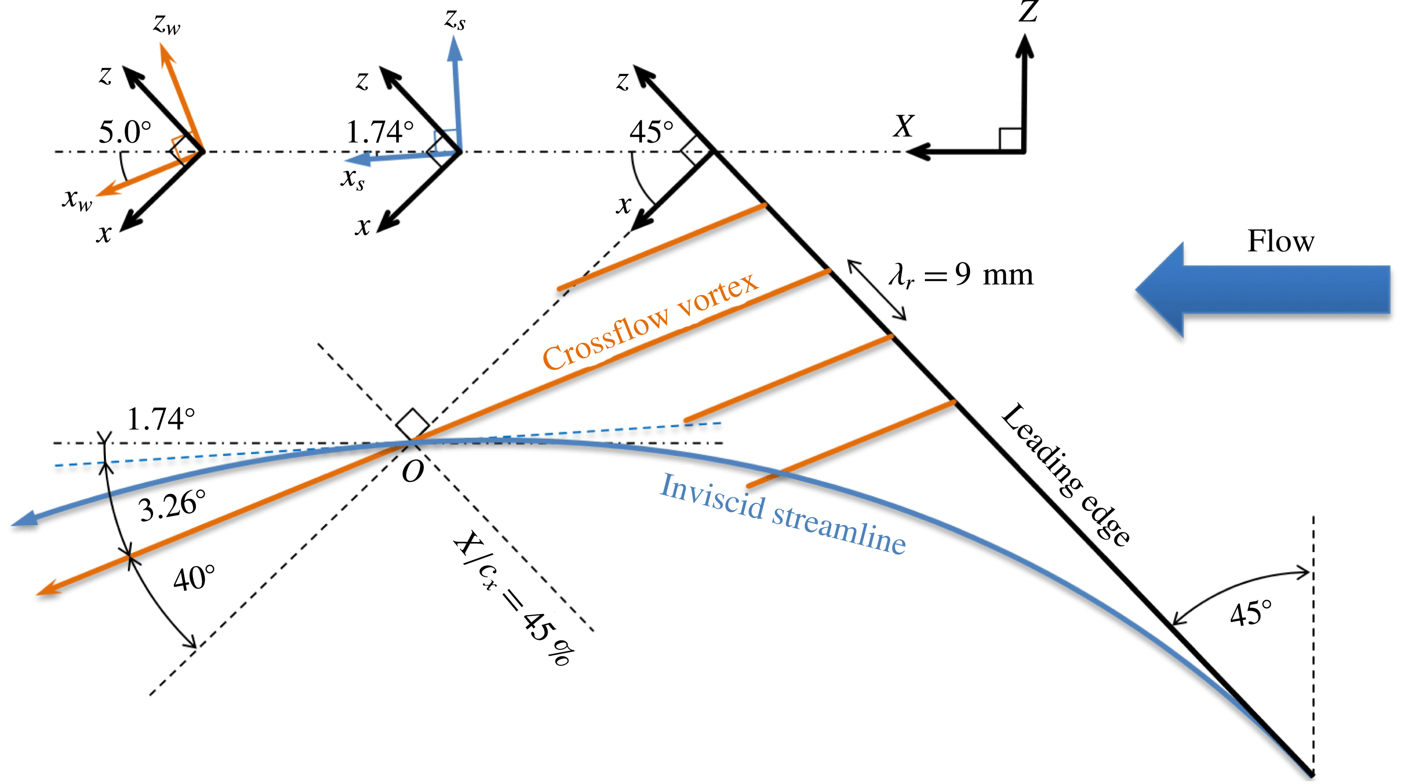
Figure 1. Definition of (left to right) crossflow-vortex-attached
 $(x_{w},z_{w})$
, inviscid-streamline-attached
$(x_{w},z_{w})$
, inviscid-streamline-attached
 $(x_{s},z_{s})$
, wing-attached
$(x_{s},z_{s})$
, wing-attached
 $(x,z)$
and tunnel-attached
$(x,z)$
and tunnel-attached
 $(X,Z)$
coordinate systems. The origin of the
$(X,Z)$
coordinate systems. The origin of the
 $(x_{w},z_{w})$
system is at
$(x_{w},z_{w})$
system is at
 $X/c_{X}=45\,\%$
. The individual coordinate system insets present the angles at the
$X/c_{X}=45\,\%$
. The individual coordinate system insets present the angles at the
 $45.6\,\%$
chord location.
$45.6\,\%$
chord location.
2 Experimental base flow
In this study, the mean velocity field obtained with three-dimensional tomo-PIV measurements is used as the base flow for the secondary stability analysis. A detailed description of the experimental set-up is given by Serpieri & Kotsonis (Reference Serpieri and Kotsonis2016). The experiment was performed in the TU Delft Low Turbulence Tunnel (LTT) facility. The model is a
 $45^{\circ }$
swept wing featuring an airfoil that is an adaptation of the NACA66018 shape, called 66018M3J, with a small leading edge radius to avoid attachment line instability. The geometric angle of attack of the wing was set to
$45^{\circ }$
swept wing featuring an airfoil that is an adaptation of the NACA66018 shape, called 66018M3J, with a small leading edge radius to avoid attachment line instability. The geometric angle of attack of the wing was set to
 $3^{\circ }$
, in order to enhance development of the crossflow instability at the pressure side, i.e. the measurement side. At this angle of attack, the pressure minimum is attained at
$3^{\circ }$
, in order to enhance development of the crossflow instability at the pressure side, i.e. the measurement side. At this angle of attack, the pressure minimum is attained at
 $X/c_{X}=63\,\%$
, where
$X/c_{X}=63\,\%$
, where
 $X$
is parallel to the tunnel walls and
$X$
is parallel to the tunnel walls and
 $c_{X}$
the chord in the
$c_{X}$
the chord in the
 $X$
-direction (
$X$
-direction (
 $c_{X}=1.27~\text{m}$
). The full
$c_{X}=1.27~\text{m}$
). The full
 $C_{p}$
-distribution is given by Serpieri & Kotsonis (Reference Serpieri and Kotsonis2016). The wind tunnel inflow velocity is
$C_{p}$
-distribution is given by Serpieri & Kotsonis (Reference Serpieri and Kotsonis2016). The wind tunnel inflow velocity is
 $\overline{Q}_{\infty }=25.6~\text{m}~\text{s}^{-1}$
, yielding Reynolds number
$\overline{Q}_{\infty }=25.6~\text{m}~\text{s}^{-1}$
, yielding Reynolds number
 $Re_{c_{X}}=2.17\times 10^{6}$
based on the chord and free-stream velocity and Mach number
$Re_{c_{X}}=2.17\times 10^{6}$
based on the chord and free-stream velocity and Mach number
 $M=0.075$
. The free-stream turbulence intensity was found to be
$M=0.075$
. The free-stream turbulence intensity was found to be
 $Tu/\overline{Q}_{\infty }=0.07\,\%$
at
$Tu/\overline{Q}_{\infty }=0.07\,\%$
at
 $\overline{Q}_{\infty }=24~\text{m}~\text{s}^{-1}$
.
$\overline{Q}_{\infty }=24~\text{m}~\text{s}^{-1}$
.
The tomo-PIV measurement is performed centred at the
 $45\,\%$
chord location in the midspan of the wing. This streamwise position is where the crossflow vortices saturate, signifying the onset of secondary instability. The slight downstream location
$45\,\%$
chord location in the midspan of the wing. This streamwise position is where the crossflow vortices saturate, signifying the onset of secondary instability. The slight downstream location
 $X/c_{X}=45.6\,\%$
is therefore considered for the stability analysis,
$X/c_{X}=45.6\,\%$
is therefore considered for the stability analysis,
 $8~\text{mm}$
downstream the origin. At that location, the vortices and inviscid streamline have an angle of
$8~\text{mm}$
downstream the origin. At that location, the vortices and inviscid streamline have an angle of
 $5.0^{\circ }$
and
$5.0^{\circ }$
and
 $1.74^{\circ }$
(counter-clockwise positive), respectively, with
$1.74^{\circ }$
(counter-clockwise positive), respectively, with
 $\overline{Q}_{\infty }$
.
$\overline{Q}_{\infty }$
.
Due to the complexity of the flow topology, several coordinate systems are defined, as illustrated in figure 1. The tunnel-attached system,
 $(X,Y,Z)$
, has
$(X,Y,Z)$
, has
 $X$
parallel to
$X$
parallel to
 $\overline{Q}_{\infty }$
,
$\overline{Q}_{\infty }$
,
 $Z$
in the spanwise direction perpendicular to the tunnel walls and
$Z$
in the spanwise direction perpendicular to the tunnel walls and
 $Y$
normal to the
$Y$
normal to the
 $ZX$
-plane. The crossflow-vortex-attached system,
$ZX$
-plane. The crossflow-vortex-attached system,
 $(x_{w},y,z_{w})$
, is aligned with the primary crossflow vortices, i.e.
$(x_{w},y,z_{w})$
, is aligned with the primary crossflow vortices, i.e.
 $x_{w}$
is parallel to the vortices,
$x_{w}$
is parallel to the vortices,
 $y$
wall normal with respect to the airfoil and
$y$
wall normal with respect to the airfoil and
 $z_{w}$
spanwise, perpendicular to the
$z_{w}$
spanwise, perpendicular to the
 $x_{w}y$
-plane. Unless otherwise specified, this will be the main coordinate system used to display the results. The related streamwise and spanwise velocity components are indicated with the subscript
$x_{w}y$
-plane. Unless otherwise specified, this will be the main coordinate system used to display the results. The related streamwise and spanwise velocity components are indicated with the subscript
 $w$
. The inviscid-streamline-attached system,
$w$
. The inviscid-streamline-attached system,
 $(x_{s},y,z_{s})$
, is aligned with the inviscid flow direction; the related streamwise and spanwise (true crossflow) velocity components have the subscript
$(x_{s},y,z_{s})$
, is aligned with the inviscid flow direction; the related streamwise and spanwise (true crossflow) velocity components have the subscript
 $s$
, i.e. the inviscid edge crossflow velocity
$s$
, i.e. the inviscid edge crossflow velocity
 $\overline{W}_{s,e}$
is zero, per definition. The wing-attached system,
$\overline{W}_{s,e}$
is zero, per definition. The wing-attached system,
 $(x,y,z)$
, is obtained by rotating the
$(x,y,z)$
, is obtained by rotating the
 $(X,Y,Z)$
-system
$(X,Y,Z)$
-system
 $45^{\circ }$
about the
$45^{\circ }$
about the
 $Y$
-axis.
$Y$
-axis.
 $x$
is orthogonal to the leading edge,
$x$
is orthogonal to the leading edge,
 $z$
parallel to the leading edge and
$z$
parallel to the leading edge and
 $y$
orthogonal to the
$y$
orthogonal to the
 $zx$
-plane. The origin of the
$zx$
-plane. The origin of the
 $(x_{w},y,z_{w})$
-system is placed at the 45 % chord, spanwise centre position. The primary instability is conditioned by installing an array of cylindrical discrete roughness elements (DRE, Reibert et al.
Reference Reibert, Saric, Carrillo and Chapman1996; Saric, Carrillo & Reibert Reference Saric, Carrillo and Reibert1998) at
$(x_{w},y,z_{w})$
-system is placed at the 45 % chord, spanwise centre position. The primary instability is conditioned by installing an array of cylindrical discrete roughness elements (DRE, Reibert et al.
Reference Reibert, Saric, Carrillo and Chapman1996; Saric, Carrillo & Reibert Reference Saric, Carrillo and Reibert1998) at
 $X/c_{X}=2.5\,\%$
parallel to the leading edge, with a spanwise spacing of
$X/c_{X}=2.5\,\%$
parallel to the leading edge, with a spanwise spacing of
 $9~\text{mm}$
along
$9~\text{mm}$
along
 $z$
, this being the naturally occurring wavelength at the transition location. The elements’ diameter and height are
$z$
, this being the naturally occurring wavelength at the transition location. The elements’ diameter and height are
 $2.8~\text{mm}\times 10~\unicode[STIX]{x03BC}\text{m}$
. The projection of the roughness spacing on the
$2.8~\text{mm}\times 10~\unicode[STIX]{x03BC}\text{m}$
. The projection of the roughness spacing on the
 $z_{w}$
-direction is
$z_{w}$
-direction is
 $9\cos 40^{\circ }=6.89~\text{mm}$
. This length is denoted by
$9\cos 40^{\circ }=6.89~\text{mm}$
. This length is denoted by
 $\unicode[STIX]{x1D706}_{r}$
and used as the primary length scale for the entirety of this work. The inviscid edge velocity in the direction of the primary vortex at
$\unicode[STIX]{x1D706}_{r}$
and used as the primary length scale for the entirety of this work. The inviscid edge velocity in the direction of the primary vortex at
 $X/c_{X}=45.6\,\%$
,
$X/c_{X}=45.6\,\%$
,
 $\overline{U}_{w,e}$
, is
$\overline{U}_{w,e}$
, is
 $28.0~\text{m}~\text{s}^{-1}$
. This is used as the velocity scale throughout this work and is denoted with
$28.0~\text{m}~\text{s}^{-1}$
. This is used as the velocity scale throughout this work and is denoted with
 $\overline{U}_{e}$
.
$\overline{U}_{e}$
.
2.1 Tomographic PIV
The tomo-PIV set-up consisted of four cameras, that were mounted in an arc configuration, located approximately one metre away from the model. The laser light enters the wind tunnel along the
 $Z$
-direction. The final field of view was
$Z$
-direction. The final field of view was
 $35\times 35\times 3~\text{mm}^{3}$
and centred at
$35\times 35\times 3~\text{mm}^{3}$
and centred at
 $X/c_{X}=45\,\%$
. Volume reconstruction and correlation were performed in a coordinate system aligned with the primary crossflow vortices, i.e. in the
$X/c_{X}=45\,\%$
. Volume reconstruction and correlation were performed in a coordinate system aligned with the primary crossflow vortices, i.e. in the
 $x_{w}$
-direction. The final interrogation volume size is
$x_{w}$
-direction. The final interrogation volume size is
 $2.6\times 0.67\times 0.67~\text{mm}^{3}$
in
$2.6\times 0.67\times 0.67~\text{mm}^{3}$
in
 $(x_{w},y,z_{w})$
, providing sufficient spatial resolution for both primary and secondary instability features. Given that PIV relies upon correlating the movement of particles in this finite interrogation volume, a spatial smoothing effect cannot be avoided, see Schrijer & Scarano (Reference Schrijer and Scarano2008). A 75 % overlap of adjacent interrogation volumes is used. The final vector field was interpolated on a grid with a
$(x_{w},y,z_{w})$
, providing sufficient spatial resolution for both primary and secondary instability features. Given that PIV relies upon correlating the movement of particles in this finite interrogation volume, a spatial smoothing effect cannot be avoided, see Schrijer & Scarano (Reference Schrijer and Scarano2008). A 75 % overlap of adjacent interrogation volumes is used. The final vector field was interpolated on a grid with a
 $0.15~\text{mm}$
spacing in all directions, only implying interpolation in
$0.15~\text{mm}$
spacing in all directions, only implying interpolation in
 $x_{w}$
.
$x_{w}$
.
The tomo-PIV measurement resolves all velocity and velocity-derivative components. Two-component hot-wire measurements covering the crossflow velocity have been reported by Deyhle & Bippes (Reference Deyhle and Bippes1996), but Bonfigli & Kloker (Reference Bonfigli and Kloker2007) emphasize the sensitivity of the stability results to the wall-normal velocity component specifically. This is also confirmed by Malik et al. (Reference Malik, Li and Chang1994). This sensitivity is confirmed by preliminary stability analyses, despite these components’ small magnitude, preluding their structural character. This is the first occasion where these data are available from experiments, rendering the two-dimensional stability approach feasible.
Uncertainties in the mean flow are heuristically linked to the maximum root-mean-square (r.m.s.) fluctuation and the number of instantaneous snapshots used for the mean flow, see Raffel et al. (Reference Raffel, Willert, Wereley and Kompenhans2007); Sciacchitano, Wieneke & Scarano (Reference Sciacchitano, Wieneke and Scarano2013). The maximum r.m.s. fluctuation has a magnitude of
 $0.1\overline{U}_{e}$
in the shear layer accommodating the type I mode. In § 4.6 the correspondence between the r.m.s. fluctuations and the type I eigenmode itself will be identified. In total, 500 uncorrelated snapshots were obtained at a sampling frequency of
$0.1\overline{U}_{e}$
in the shear layer accommodating the type I mode. In § 4.6 the correspondence between the r.m.s. fluctuations and the type I eigenmode itself will be identified. In total, 500 uncorrelated snapshots were obtained at a sampling frequency of
 $0.5~\text{Hz}$
. The number of instantaneous frames in the ensemble will be denoted by
$0.5~\text{Hz}$
. The number of instantaneous frames in the ensemble will be denoted by
 $N_{fr}$
. When less than 500, the individual snapshots are randomly selected from the total pool. The uncertainty of the mean field is estimated to be
$N_{fr}$
. When less than 500, the individual snapshots are randomly selected from the total pool. The uncertainty of the mean field is estimated to be
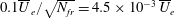 $0.1\overline{U}_{e}/\sqrt{N_{fr}}=4.5\times 10^{-3}\,\overline{U}_{e}$
for the
$0.1\overline{U}_{e}/\sqrt{N_{fr}}=4.5\times 10^{-3}\,\overline{U}_{e}$
for the
 $N_{fr}=500$
case. As will be demonstrated, this is a high uncertainty with respect to the sensitivity of the stability analysis. Previous studies, see Groot et al. (Reference Groot, Ye, van Oudheusden, Zhang and Pinna2016), demonstrated sufficient convergence of the stability results with a similar ensemble size as used here. A formal study on the convergence with
$N_{fr}=500$
case. As will be demonstrated, this is a high uncertainty with respect to the sensitivity of the stability analysis. Previous studies, see Groot et al. (Reference Groot, Ye, van Oudheusden, Zhang and Pinna2016), demonstrated sufficient convergence of the stability results with a similar ensemble size as used here. A formal study on the convergence with
 $N_{fr}$
is considered in § 4.2.
$N_{fr}$
is considered in § 4.2.
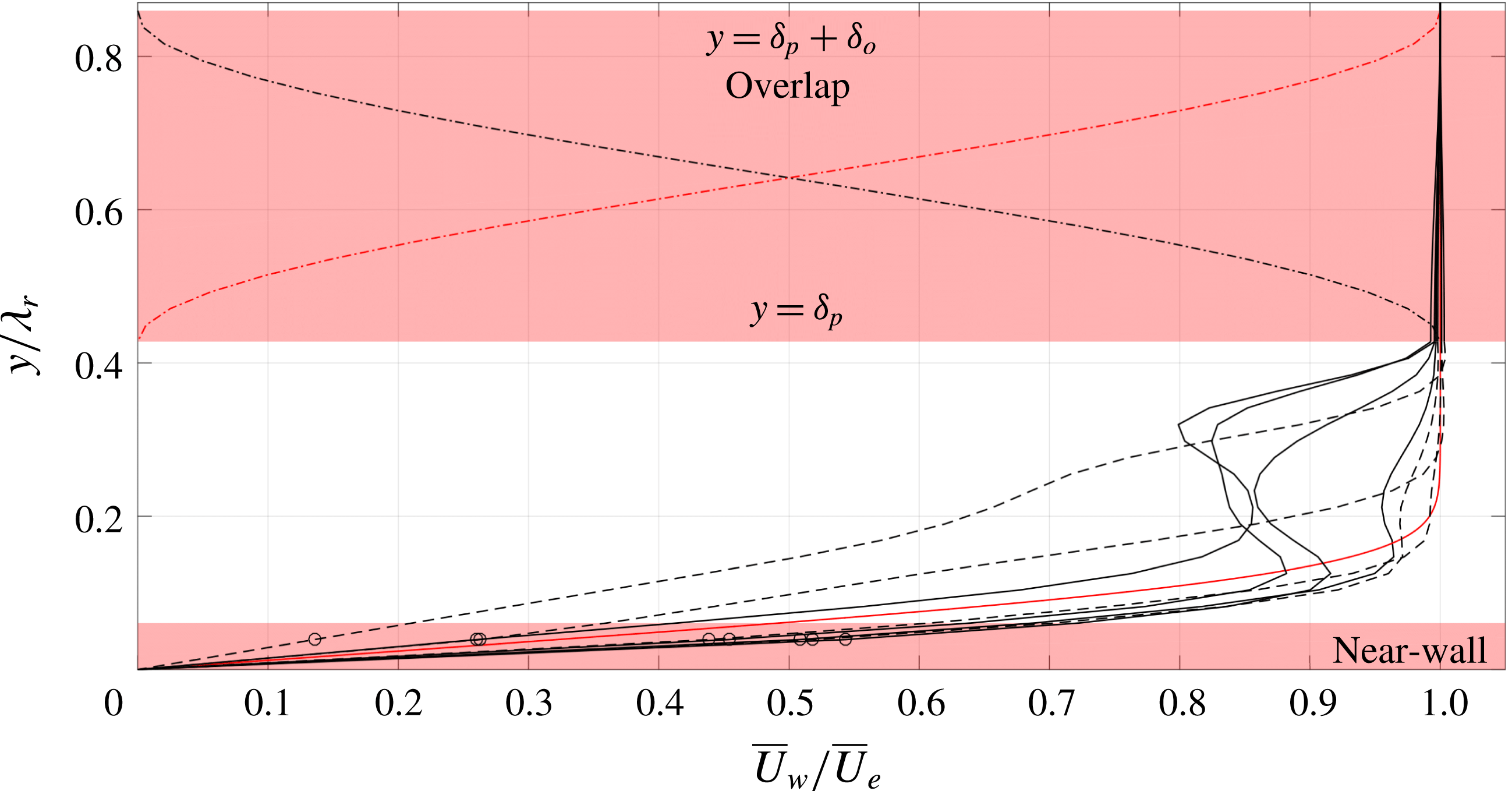
Figure 2. Overlap and near-wall region, illustrating cosine weights (dash-dotted lines) for the rotated Blasius (red solid) and base flow profiles (black solid leeward, dashed windward with respect to
 $\overline{W}_{w}$
). Interpolated points in the near-wall region (circles).
$\overline{W}_{w}$
). Interpolated points in the near-wall region (circles).
Finally, proper orthogonal decomposition (POD) analysis is applied to identify the most energetic spatially correlated three-dimensional flow structures, using the snapshot technique introduced by Sirovich (Reference Sirovich1987). A detailed description of the POD results is given in Serpieri & Kotsonis (Reference Serpieri and Kotsonis2016). For the present study, access to the three-dimensional POD modes is indispensable as it enables topological validation of the applied stability analysis; as presented in § 4.6.
2.2 Pre-processing for stability analysis
Due to the aforementioned sensitivity of the stability results on variations of the base flow, a pre-processing strategy is followed in regard to the mean flow fields. This processing is mainly related to the limited field of view and measurement uncertainty associated with measuring in close proximity to the wall, inherent to tomo-PIV.
Although the stability eigenmodes of interest decay exponentially in the wall-normal direction, see Schmid & Henningson (Reference Schmid and Henningson2001), the truncation boundary in this direction must be placed high enough to preclude artificial effects, see Grosch & Orszag (Reference Grosch and Orszag1977), Sandstede & Scheel (Reference Sandstede and Scheel2000). To this end, the
 $\overline{U}_{w}$
and
$\overline{U}_{w}$
and
 $\overline{W}_{w}$
base flow velocity components are extrapolated using the Blasius solution in the inviscid streamline direction, i.e.
$\overline{W}_{w}$
base flow velocity components are extrapolated using the Blasius solution in the inviscid streamline direction, i.e.
 $\overline{W}_{w,e}=\overline{U}_{w,e}\tan 3.26^{\circ }=1.59~\text{m}~\text{s}^{-1}$
. An approximation with a Falkner–Skan–Cooke profile would be better, but the field of view extends to such heights, approximately 2 undisturbed boundary layer thicknesses as shown in figure 2, that this approach is deemed sufficient. As expected, the Blasius solution and the PIV dataset do not match exactly at the top of the field of view. Therefore, a cosine weight overlap layer is introduced to make the resulting base flow continuous at the interface. The height up to which the PIV data are unaffected is denoted by
$\overline{W}_{w,e}=\overline{U}_{w,e}\tan 3.26^{\circ }=1.59~\text{m}~\text{s}^{-1}$
. An approximation with a Falkner–Skan–Cooke profile would be better, but the field of view extends to such heights, approximately 2 undisturbed boundary layer thicknesses as shown in figure 2, that this approach is deemed sufficient. As expected, the Blasius solution and the PIV dataset do not match exactly at the top of the field of view. Therefore, a cosine weight overlap layer is introduced to make the resulting base flow continuous at the interface. The height up to which the PIV data are unaffected is denoted by
 $\unicode[STIX]{x1D6FF}_{p}$
and the height of the overlap region by
$\unicode[STIX]{x1D6FF}_{p}$
and the height of the overlap region by
 $\unicode[STIX]{x1D6FF}_{o}$
, see figure 2.
$\unicode[STIX]{x1D6FF}_{o}$
, see figure 2.
 $\overline{V}$
is extrapolated in a similar way, approaching zero in the free stream.
$\overline{V}$
is extrapolated in a similar way, approaching zero in the free stream.
A second aspect requiring attention is the PIV fidelity in the near-wall region. Near-wall PIV measurements are subject to a number of decremental factors such as laser-light reflections, low particle density and the strong shear, see Scarano (Reference Scarano2001). Effectively, these features result in a deviation of the velocity profile from the no-slip condition. The type III mode is dominant in this region and therefore expected to depend on the near-wall details of the flow. The PIV uncertainty in the near-wall region is judged to render the use of the base flow for the extraction of the type III mode more challenging. While such objective lies out of the scope of the current work, technical improvements on the tomo-PIV technique could enable the resolution of near-wall modes in future explorations. For the present study, the proper secondary modes of type I and II will be considered.
The near-wall region is approached in 2 steps. First, the profiles are connected to the wall by linear extrapolation; artificially imposing the no-slip condition. As a second step, the data at the
 $y$
-coordinate closest to the wall are overwritten with an interpolation. As such, the no-slip condition is connected smoothly to the data on the second non-zero
$y$
-coordinate closest to the wall are overwritten with an interpolation. As such, the no-slip condition is connected smoothly to the data on the second non-zero
 $y$
-coordinate,
$y$
-coordinate,
 $y/\unicode[STIX]{x1D706}_{r}=0.061$
, designating the near-wall region, see figure 2. The modes of type I and II are found to be affected negligibly by this kind of base flow changes outside their spatial region of dominance, see § 4.4.
$y/\unicode[STIX]{x1D706}_{r}=0.061$
, designating the near-wall region, see figure 2. The modes of type I and II are found to be affected negligibly by this kind of base flow changes outside their spatial region of dominance, see § 4.4.
A third and final aspect is the fact that the in-plane flow is not divergence free, i.e.
 $\unicode[STIX]{x2202}\overline{V}/\unicode[STIX]{x2202}y+\unicode[STIX]{x2202}\overline{W}_{w}/\unicode[STIX]{x2202}z_{w}\neq 0$
. As will be indicated in § 3, this is an implicit assumption in the stability approach and can have an impact on the precise growth rate values. Bonfigli & Kloker (Reference Bonfigli and Kloker2007) discuss a treatment, where the
$\unicode[STIX]{x2202}\overline{V}/\unicode[STIX]{x2202}y+\unicode[STIX]{x2202}\overline{W}_{w}/\unicode[STIX]{x2202}z_{w}\neq 0$
. As will be indicated in § 3, this is an implicit assumption in the stability approach and can have an impact on the precise growth rate values. Bonfigli & Kloker (Reference Bonfigli and Kloker2007) discuss a treatment, where the
 $\unicode[STIX]{x2202}\overline{V}/\unicode[STIX]{x2202}y$
- and
$\unicode[STIX]{x2202}\overline{V}/\unicode[STIX]{x2202}y$
- and
 $\unicode[STIX]{x2202}\overline{W}_{w}/\unicode[STIX]{x2202}z_{w}$
-fields are integrated to obtain the
$\unicode[STIX]{x2202}\overline{W}_{w}/\unicode[STIX]{x2202}z_{w}$
-fields are integrated to obtain the
 $\overline{W}$
and
$\overline{W}$
and
 $\overline{V}$
fields, respectively. Given the fields in the near-wall region are fitted with the aforementioned approach, integrating the
$\overline{V}$
fields, respectively. Given the fields in the near-wall region are fitted with the aforementioned approach, integrating the
 $\unicode[STIX]{x2202}\overline{V}/\unicode[STIX]{x2202}y$
- and
$\unicode[STIX]{x2202}\overline{V}/\unicode[STIX]{x2202}y$
- and
 $\unicode[STIX]{x2202}\overline{W}_{w}/\unicode[STIX]{x2202}z_{w}$
-fields, which are experimentally measured data that are already differentiated, is expected to yield unreliable results. A better approach to enforce the divergence-free condition on the measured in-plane flow data is to perform solenoidal interpolation, see Vedula & Adrian (Reference Vedula and Adrian2005). Several approaches on the treatment of PIV data to yield a closer match with the equations governing fluid flow have been proposed, for example see Gesemann et al. (Reference Gesemann, Huhn, Schanz and Schröder2016), Schneiders & Scarano (Reference Schneiders and Scarano2016), however, the main aim of this study is to identify whether stability results can be extracted from PIV mean flows in the first place. As shown by Bonfigli & Kloker (Reference Bonfigli and Kloker2007), the induced change in the growth rates by considering either the
$\unicode[STIX]{x2202}\overline{W}_{w}/\unicode[STIX]{x2202}z_{w}$
-fields, which are experimentally measured data that are already differentiated, is expected to yield unreliable results. A better approach to enforce the divergence-free condition on the measured in-plane flow data is to perform solenoidal interpolation, see Vedula & Adrian (Reference Vedula and Adrian2005). Several approaches on the treatment of PIV data to yield a closer match with the equations governing fluid flow have been proposed, for example see Gesemann et al. (Reference Gesemann, Huhn, Schanz and Schröder2016), Schneiders & Scarano (Reference Schneiders and Scarano2016), however, the main aim of this study is to identify whether stability results can be extracted from PIV mean flows in the first place. As shown by Bonfigli & Kloker (Reference Bonfigli and Kloker2007), the induced change in the growth rates by considering either the
 $\overline{V}$
- or
$\overline{V}$
- or
 $\overline{W}_{w}$
-fixed approach is noticeable, in particular for the type I instability, but it does not oppose extracting the growth’s order of magnitude. It will be shown in § 4.3 that the expected induced differences lie within the established bounds of uncertainty.
$\overline{W}_{w}$
-fixed approach is noticeable, in particular for the type I instability, but it does not oppose extracting the growth’s order of magnitude. It will be shown in § 4.3 that the expected induced differences lie within the established bounds of uncertainty.
2.3 Distorted base flow and shear fields
An analysis of the PIV mean flow is described in this section, to distill expectations for the stability results based on the literature. The resulting velocity fields, confined to the measurement domain, are shown in figure 3, which is equivalent to figure 18 of Serpieri & Kotsonis (Reference Serpieri and Kotsonis2016), but differs in streamwise location and orientation. Two spanwise neighbouring stationary crossflow vortices are given. The two vortices have slightly different strengths, which is possibly a result of minute discrepancies between the individual DREs responsible for the conditioning of these vortices in the receptivity region near the leading edge. While this is an unavoidable effect of experimental conditions, it presents a convenient and realistic opportunity in demonstrating the effect of the base flow, i.e. the amplitude of the primary crossflow vortex, on the secondary instability characteristics (Wassermann & Kloker Reference Wassermann and Kloker2002; Serpieri & Kotsonis Reference Serpieri and Kotsonis2018). The two vortices are analysed separately, limiting the spanwise domain length to
 $1\unicode[STIX]{x1D706}_{r}=6.89~\text{mm}$
as indicated in figure 3.
$1\unicode[STIX]{x1D706}_{r}=6.89~\text{mm}$
as indicated in figure 3.
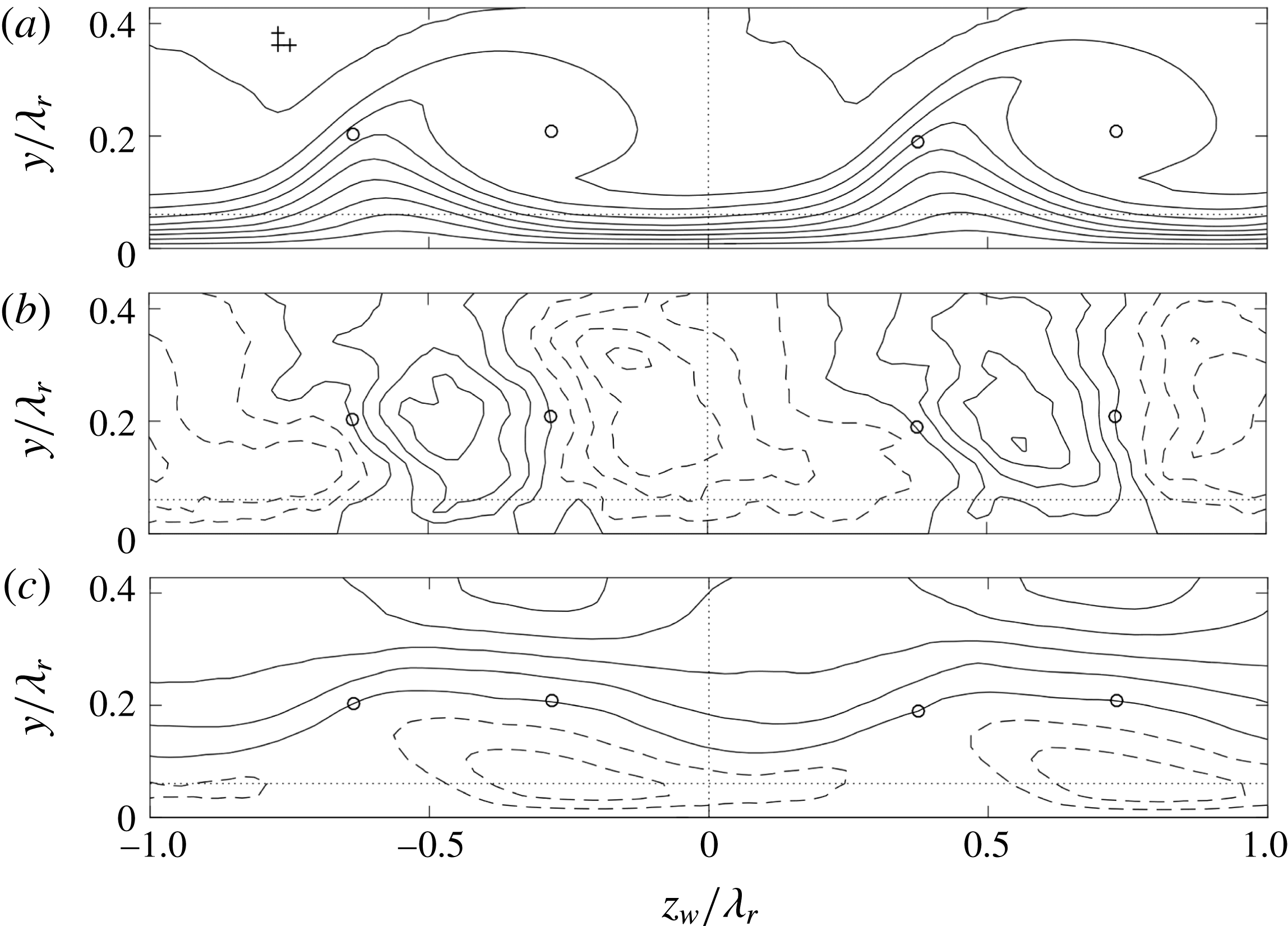
Figure 3. (a)
 $\overline{U}_{w}/\overline{U}_{e}$
(10 levels, from 0 to 1), (b)
$\overline{U}_{w}/\overline{U}_{e}$
(10 levels, from 0 to 1), (b)
 $\overline{V}/\overline{U}_{e}$
(11 levels, from
$\overline{V}/\overline{U}_{e}$
(11 levels, from
 $-0.02$
to
$-0.02$
to
 $0.02$
) and (c)
$0.02$
) and (c)
 $\overline{W}_{w}/\overline{U}_{e}$
(11 levels, from
$\overline{W}_{w}/\overline{U}_{e}$
(11 levels, from
 $-0.05$
to
$-0.05$
to
 $0.05$
) at constant
$0.05$
) at constant
 $x_{w}$
(
$x_{w}$
(
 $x=45.6\,\%$
chord at
$x=45.6\,\%$
chord at
 $z_{w}/\unicode[STIX]{x1D706}_{r}=0$
), negative contours are dashed. Spatial resolution of experimental data (pluses,
$z_{w}/\unicode[STIX]{x1D706}_{r}=0$
), negative contours are dashed. Spatial resolution of experimental data (pluses,
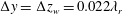 $\unicode[STIX]{x0394}y=\unicode[STIX]{x0394}z_{w}=0.022\unicode[STIX]{x1D706}_{r}$
),
$\unicode[STIX]{x0394}y=\unicode[STIX]{x0394}z_{w}=0.022\unicode[STIX]{x1D706}_{r}$
),
 $(\overline{V},\overline{W}_{w})$
-field centre and saddle point locations (circles, (
$(\overline{V},\overline{W}_{w})$
-field centre and saddle point locations (circles, (
 $z_{w}$
,
$z_{w}$
,
 $y$
)
$y$
)
 $/\unicode[STIX]{x1D706}_{r}=(0.364;0.202)-(1,0)$
,
$/\unicode[STIX]{x1D706}_{r}=(0.364;0.202)-(1,0)$
,
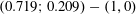 $(0.719;0.209)-(1,0)$
,
$(0.719;0.209)-(1,0)$
,
 $(0.374;0.190)$
and
$(0.374;0.190)$
and
 $(0.731;0.209)$
), domain separation for strong (right) and weak (left) vortex (vertical dotted line
$(0.731;0.209)$
), domain separation for strong (right) and weak (left) vortex (vertical dotted line
 $z_{w}/\unicode[STIX]{x1D706}_{r}=0$
), near-wall region (horizontal dotted line
$z_{w}/\unicode[STIX]{x1D706}_{r}=0$
), near-wall region (horizontal dotted line
 $y/\unicode[STIX]{x1D706}_{r}\leqslant 0.061$
).
$y/\unicode[STIX]{x1D706}_{r}\leqslant 0.061$
).
A measure for the primary disturbance amplitude based on the measured mean velocity profiles was introduced by Fischer & Dallmann (Reference Fischer and Dallmann1991):
 $$\begin{eqnarray}\displaystyle & \displaystyle {\textstyle \frac{1}{2}}\max _{y}\left(\max _{z_{w}}\overline{U}_{s}(z_{w},y)-\min _{z_{w}}\overline{U}_{s}(z_{w},y)\right), & \displaystyle\end{eqnarray}$$
where the subscript
 $s$
denotes the inviscid-streamline-attached coordinate system. Using the separate spanwise domains for the two vortices, this yields 28.7 % and 27.3 % for the strong and weak vortex, respectively, with respect to
$s$
denotes the inviscid-streamline-attached coordinate system. Using the separate spanwise domains for the two vortices, this yields 28.7 % and 27.3 % for the strong and weak vortex, respectively, with respect to
 $\overline{U}_{e}$
. Scaling with the edge value of
$\overline{U}_{e}$
. Scaling with the edge value of
 $\overline{U}_{s}$
yields the same numbers to the given precision, thus this distinction is omitted in the remainder. Based on their modelling assumptions and the aforementioned measure, Fischer et al. (Reference Fischer, Hein and Dallmann1993) observe high-frequency secondary instabilities for disturbance amplitudes beyond 11 %
$\overline{U}_{s}$
yields the same numbers to the given precision, thus this distinction is omitted in the remainder. Based on their modelling assumptions and the aforementioned measure, Fischer et al. (Reference Fischer, Hein and Dallmann1993) observe high-frequency secondary instabilities for disturbance amplitudes beyond 11 %
 $\overline{U}_{e}$
. Wassermann & Kloker (Reference Wassermann and Kloker2002) (cf. page 75) report that the onset of the secondary instability to the maximal in-plane deceleration imposed by the mean flow distortion is equal to 30 %
$\overline{U}_{e}$
. Wassermann & Kloker (Reference Wassermann and Kloker2002) (cf. page 75) report that the onset of the secondary instability to the maximal in-plane deceleration imposed by the mean flow distortion is equal to 30 %
 $\overline{U}_{e}$
, based on their DNS. The Reynolds number in both references is approximately half that considered here, but these values can still act as an order-of-magnitude check for the current purposes. In the current experiment, the perturbations on the weaker vortex are much weaker than on the strong vortex, so also the instability is expected to be weaker in terms of a lower growth rate.
$\overline{U}_{e}$
, based on their DNS. The Reynolds number in both references is approximately half that considered here, but these values can still act as an order-of-magnitude check for the current purposes. In the current experiment, the perturbations on the weaker vortex are much weaker than on the strong vortex, so also the instability is expected to be weaker in terms of a lower growth rate.
The magnitude of the components in the
 $z_{w}y$
-plane is condensed in a similar way:
$z_{w}y$
-plane is condensed in a similar way:
 $$\begin{eqnarray}\displaystyle & \displaystyle {\textstyle \frac{1}{2}}\max _{y}\left(\max _{z_{w}}\overline{V}(z_{w},y)-\min _{z_{w}}\overline{V}(z_{w},y)\right), & \displaystyle\end{eqnarray}$$
 $$\begin{eqnarray}\displaystyle & \displaystyle {\textstyle \frac{1}{2}}\max _{z_{w}}\left(\max _{y}\overline{W}_{w}(z_{w},y)-\min _{y}\overline{W}_{w}(z_{w},y)\right). & \displaystyle\end{eqnarray}$$
The
 $z_{w}$
-component is considered instead of the
$z_{w}$
-component is considered instead of the
 $z_{s}$
-component, because the former appears in the stability problem. One obtains 1.48 % and 1.51 % for
$z_{s}$
-component, because the former appears in the stability problem. One obtains 1.48 % and 1.51 % for
 $\overline{V}$
for the strong and weak vortices, respectively, with respect to
$\overline{V}$
for the strong and weak vortices, respectively, with respect to
 $\overline{U}_{e}$
. This component is evidently quite insensitive to variations in the spanwise direction. For
$\overline{U}_{e}$
. This component is evidently quite insensitive to variations in the spanwise direction. For
 $\overline{W}_{w}$
, values of 4.78 % and 4.22 % for the strong and weak vortex are observed, respectively. In terms of absolute size, the in-plane velocity components change negligibly as opposed to the streamwise velocity component.
$\overline{W}_{w}$
, values of 4.78 % and 4.22 % for the strong and weak vortex are observed, respectively. In terms of absolute size, the in-plane velocity components change negligibly as opposed to the streamwise velocity component.
Figure 4. (a) In-plane
 $\overline{U}_{w}$
-shear magnitude of the strong vortex for
$\overline{U}_{w}$
-shear magnitude of the strong vortex for
 $N_{fr}=500$
(levels from 0 to 7 with steps of 0.5 in
$N_{fr}=500$
(levels from 0 to 7 with steps of 0.5 in
 $\overline{U}_{e}/\unicode[STIX]{x1D706}_{r}$
-units, level
$\overline{U}_{e}/\unicode[STIX]{x1D706}_{r}$
-units, level
 $7\,\overline{U}_{e}/\unicode[STIX]{x1D706}_{r}$
is dashed). Position of
$7\,\overline{U}_{e}/\unicode[STIX]{x1D706}_{r}$
is dashed). Position of
 $(\overline{V},\overline{W}_{w})$
-field saddle point (solid circle),
$(\overline{V},\overline{W}_{w})$
-field saddle point (solid circle),
 $\unicode[STIX]{x2202}\overline{U}_{w}/\unicode[STIX]{x2202}z_{w}$
-minimum (solid square) and type I
$\unicode[STIX]{x2202}\overline{U}_{w}/\unicode[STIX]{x2202}z_{w}$
-minimum (solid square) and type I
 $|\tilde{u} _{w}|$
-maximum (dash-dotted lines). (b)
$|\tilde{u} _{w}|$
-maximum (dash-dotted lines). (b)
 $y$
- and (c)
$y$
- and (c)
 $z_{w}$
-profiles of
$z_{w}$
-profiles of
 $\unicode[STIX]{x2202}\overline{U}_{w}/\unicode[STIX]{x2202}z_{w}$
(circles) and
$\unicode[STIX]{x2202}\overline{U}_{w}/\unicode[STIX]{x2202}z_{w}$
(circles) and
 $\unicode[STIX]{x2202}\overline{U}_{w}/\unicode[STIX]{x2202}y$
(squares) for
$\unicode[STIX]{x2202}\overline{U}_{w}/\unicode[STIX]{x2202}y$
(squares) for
 $N_{fr}=500$
(symbols), 400 (solid line) and 300 (dashed line) along the dash-dotted lines in (a). Near-wall region (
$N_{fr}=500$
(symbols), 400 (solid line) and 300 (dashed line) along the dash-dotted lines in (a). Near-wall region (
 $y/\unicode[STIX]{x1D706}_{r}\leqslant 0.061$
) and upper limit PIV domain (
$y/\unicode[STIX]{x1D706}_{r}\leqslant 0.061$
) and upper limit PIV domain (
 $y/\unicode[STIX]{x1D706}_{r}=0.433$
) (dotted lines).
$y/\unicode[STIX]{x1D706}_{r}=0.433$
) (dotted lines).
The total in-plane
 $\overline{U}_{w}$
-shear magnitude of the strong vortex corresponding to the
$\overline{U}_{w}$
-shear magnitude of the strong vortex corresponding to the
 $N_{fr}=500$
mean tomo-PIV flow field is shown in figure 4(a). This is displayed on the mapped Chebyshev grid that is ultimately used to perform the stability analysis; this grid will be introduced in § 3.3. The height of the measurement domain and the near-wall region are illustrated in figure 4(a,b). Sixth-order finite differences are used to determine the derivative fields consistently, i.e. using central differences in the interior and forward/backward differences at the boundaries. Differentiating PIV data with high-order finite differences is generally discouraged as random errors could result, see Foucaut & Stanislas (Reference Foucaut and Stanislas2002). The high order was chosen to reduce the truncation error corresponding to the finite spatial resolution of the tomo-PIV. Using lower-order finite differences for the derivatives fields affected the results negligibly, see § 4.2.
$N_{fr}=500$
mean tomo-PIV flow field is shown in figure 4(a). This is displayed on the mapped Chebyshev grid that is ultimately used to perform the stability analysis; this grid will be introduced in § 3.3. The height of the measurement domain and the near-wall region are illustrated in figure 4(a,b). Sixth-order finite differences are used to determine the derivative fields consistently, i.e. using central differences in the interior and forward/backward differences at the boundaries. Differentiating PIV data with high-order finite differences is generally discouraged as random errors could result, see Foucaut & Stanislas (Reference Foucaut and Stanislas2002). The high order was chosen to reduce the truncation error corresponding to the finite spatial resolution of the tomo-PIV. Using lower-order finite differences for the derivatives fields affected the results negligibly, see § 4.2.
As discussed earlier, conditions on the required base flow accuracy are case dependent and hence difficult to set in general. It is commonly suggested that the base flow should satisfy the Navier–Stokes equations to extreme accuracy, see Reed et al. (Reference Reed, Saric and Arnal1996) and Theofilis (Reference Theofilis2003). The work of Ehrenstein & Gallaire (Reference Ehrenstein and Gallaire2005) and Alizard & Robinet (Reference Alizard and Robinet2007) reflect this requirement through their use of Navier–Stokes over Blasius solutions for the flat-plate boundary layer flow. Arnal (Reference Arnal1994) shows the maximum shear values must be represented accurately in the case of inviscid inflectional instabilities. To identify how well this criterion is satisfied in the current case, the position of a baseline type I eigenfunction maximum is identified in figure 4(a) by the dash-dotted lines
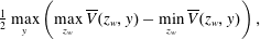
 $z_{w}/\unicode[STIX]{x1D706}_{r}=0.378$
and
$z_{w}/\unicode[STIX]{x1D706}_{r}=0.378$
and
 $y/\unicode[STIX]{x1D706}_{r}=0.223$
. Figure 4(b,c) displays both derivative profiles
$y/\unicode[STIX]{x1D706}_{r}=0.223$
. Figure 4(b,c) displays both derivative profiles
 $\unicode[STIX]{x2202}\overline{U}_{w}/\unicode[STIX]{x2202}y$
and
$\unicode[STIX]{x2202}\overline{U}_{w}/\unicode[STIX]{x2202}y$
and
 $\unicode[STIX]{x2202}\overline{U}_{w}/\unicode[STIX]{x2202}z_{w}$
along these lines, respectively. Next to the profiles for
$\unicode[STIX]{x2202}\overline{U}_{w}/\unicode[STIX]{x2202}z_{w}$
along these lines, respectively. Next to the profiles for
 $N_{fr}=500$
, those corresponding to
$N_{fr}=500$
, those corresponding to
 $N_{fr}=400$
and 300 (single random samplings) are shown. The derivative profiles are found to be nearly identical. At the inflection point location, the differences in the shear magnitudes do not exceed 1.1 %. In the near-wall region, the largest deviation is found to be 2.3 %.
$N_{fr}=400$
and 300 (single random samplings) are shown. The derivative profiles are found to be nearly identical. At the inflection point location, the differences in the shear magnitudes do not exceed 1.1 %. In the near-wall region, the largest deviation is found to be 2.3 %.

Figure 5. (a) In-plane
 $\overline{U}_{w}$
-shear magnitude of the weak vortex (solid contours) for
$\overline{U}_{w}$
-shear magnitude of the weak vortex (solid contours) for
 $N_{fr}=500$
(levels from 0 to 5 with steps of 1 in
$N_{fr}=500$
(levels from 0 to 5 with steps of 1 in
 $\overline{U}_{e}/\unicode[STIX]{x1D706}_{r}$
-units, level
$\overline{U}_{e}/\unicode[STIX]{x1D706}_{r}$
-units, level
 $5\,\overline{U}_{e}/\unicode[STIX]{x1D706}_{r}$
is dash-dotted). Position of
$5\,\overline{U}_{e}/\unicode[STIX]{x1D706}_{r}$
is dash-dotted). Position of
 $(\overline{V},\overline{W}_{w})$
-field saddle point (solid circle),
$(\overline{V},\overline{W}_{w})$
-field saddle point (solid circle),
 $\unicode[STIX]{x2202}\overline{U}_{w}/\unicode[STIX]{x2202}z_{w}$
-minimum (solid square) and type I
$\unicode[STIX]{x2202}\overline{U}_{w}/\unicode[STIX]{x2202}z_{w}$
-minimum (solid square) and type I
 $|\tilde{u} _{w}|$
-maximum (solid lines). (b)
$|\tilde{u} _{w}|$
-maximum (solid lines). (b)
 $y$
- and (c)
$y$
- and (c)
 $z_{w}$
-profiles of
$z_{w}$
-profiles of
 $\unicode[STIX]{x2202}\overline{U}_{w}/\unicode[STIX]{x2202}z_{w}$
(circles) and
$\unicode[STIX]{x2202}\overline{U}_{w}/\unicode[STIX]{x2202}z_{w}$
(circles) and
 $\unicode[STIX]{x2202}\overline{U}_{w}/\unicode[STIX]{x2202}y$
(squares) along the straight solid lines in (a). Strong vortex equivalents of the shear profiles and eigenfunction maximum position are given by dashed lines.
$\unicode[STIX]{x2202}\overline{U}_{w}/\unicode[STIX]{x2202}y$
(squares) along the straight solid lines in (a). Strong vortex equivalents of the shear profiles and eigenfunction maximum position are given by dashed lines.
The total in-plane shear of the weaker vortex shown to the left in figure 3 is compared to that associated with the stronger vortex in figure 5. Note that the contours below
 $y/\unicode[STIX]{x1D706}_{r}=0.15$
near the spanwise domain boundaries are very close for the different vortices. The shear layer of the weaker vortex protrudes less into the free stream. In figure 5(c), this effect manifests itself as a shift of the shear profiles in the negative
$y/\unicode[STIX]{x1D706}_{r}=0.15$
near the spanwise domain boundaries are very close for the different vortices. The shear layer of the weaker vortex protrudes less into the free stream. In figure 5(c), this effect manifests itself as a shift of the shear profiles in the negative
 $z_{w}$
-direction. The profiles shown in both figures 4(b,c) and 5(b,c) suggest the maximum of the type I eigenfunction (
$z_{w}$
-direction. The profiles shown in both figures 4(b,c) and 5(b,c) suggest the maximum of the type I eigenfunction (
 $(z_{w},y)/\unicode[STIX]{x1D706}_{r}=(0.378;0.223)$
and
$(z_{w},y)/\unicode[STIX]{x1D706}_{r}=(0.378;0.223)$
and
 $(0.367;0.223)$
, respectively) lies close to the overall minimum of the
$(0.367;0.223)$
, respectively) lies close to the overall minimum of the
 $\unicode[STIX]{x2202}\overline{U}_{w}/\unicode[STIX]{x2202}z_{w}$
shear component. The symbols in figures 4(a) and 5(a) illustrate the latter point (
$\unicode[STIX]{x2202}\overline{U}_{w}/\unicode[STIX]{x2202}z_{w}$
shear component. The symbols in figures 4(a) and 5(a) illustrate the latter point (
 $(z_{w},y)/\unicode[STIX]{x1D706}_{r}=(0.314;0.162)$
and
$(z_{w},y)/\unicode[STIX]{x1D706}_{r}=(0.314;0.162)$
and
 $(0.300;0.153)$
, respectively), in fact, lies quite far. In both cases, it consistently lies slightly above the saddle point in the in-plane velocity field imposed by
$(0.300;0.153)$
, respectively), in fact, lies quite far. In both cases, it consistently lies slightly above the saddle point in the in-plane velocity field imposed by
 $\overline{V}$
and
$\overline{V}$
and
 $\overline{W}_{w}$
.
$\overline{W}_{w}$
.
In conclusion, both vortices are expected to be unstable to secondary instabilities based on the results of Fischer et al. (Reference Fischer, Hein and Dallmann1993). The weaker vortex, as opposed to the stronger, is expected to yield a smaller growth rate, which is mainly caused by changes in the streamwise velocity component. The in-plane velocity components vary marginally with respect to the streamwise component, resulting in a relatively larger magnitude on the weak vortex, which amplifies the type I instability, while weakening the type II instability (Bonfigli & Kloker Reference Bonfigli and Kloker2007). Moreover, the in-plane location of the maximum amplitude of the type I mode seems to be fixed in close proximity of the saddle point of the in-plane flow. The derivative fields display small discrepancies with changing
 $N_{fr}$
, being a first requirement for a successful stability analysis (Arnal Reference Arnal1994).
$N_{fr}$
, being a first requirement for a successful stability analysis (Arnal Reference Arnal1994).
3 Spanwise global stability analysis
3.1 Formulation
The stability approach accounts for all flow inhomogeneities in a two-dimensional plane. The flow is assumed to be invariant in the third direction. Based on their topological features, the best choice for the invariant direction in the case of the primary crossflow vortices is orthogonal to the wave vector of the primary vortices: the
 $x_{w}$
-direction. Implicitly, the curvature of the vortices is neglected, which is a posteriori justified by the small wavelengths of the secondary modes, see Malik et al. (Reference Malik, Li, Choudhari and Chang1999), Theofilis (Reference Theofilis2003) and Bonfigli & Kloker (Reference Bonfigli and Kloker2007) for more details.
$x_{w}$
-direction. Implicitly, the curvature of the vortices is neglected, which is a posteriori justified by the small wavelengths of the secondary modes, see Malik et al. (Reference Malik, Li, Choudhari and Chang1999), Theofilis (Reference Theofilis2003) and Bonfigli & Kloker (Reference Bonfigli and Kloker2007) for more details.
Care should be taken in defining boundary conditions on the introduced domain boundaries. The domain is confined to either one of the two vortices shown in figure 3, depending on the investigated case. For a semi-infinite swept wing at canonical conditions, the flow is periodic in the leading edge parallel
 $z$
-coordinate. This suggests considering the
$z$
-coordinate. This suggests considering the
 $zy$
-plane for the stability analysis and justifies applying periodic boundary conditions. The
$zy$
-plane for the stability analysis and justifies applying periodic boundary conditions. The
 $x_{w}$
-direction is non-orthogonal to the
$x_{w}$
-direction is non-orthogonal to the
 $zy$
-plane, which can be accounted for by projecting the velocity vectors in the
$zy$
-plane, which can be accounted for by projecting the velocity vectors in the
 $zy$
-plane onto the
$zy$
-plane onto the
 $z_{w}y$
-plane. Bonfigli & Kloker (Reference Bonfigli and Kloker2007) go into high detail describing a similar approach, illustrating the requirement for a correction concerning flow continuity.
$z_{w}y$
-plane. Bonfigli & Kloker (Reference Bonfigli and Kloker2007) go into high detail describing a similar approach, illustrating the requirement for a correction concerning flow continuity.
In the present work, the choice is made not to adhere to the most periodic spanwise direction. The
 $z_{w}y$
-planes were extracted directly from the tomo-PIV data, since the PIV cross-correlation is performed in this direction and hence yields the most consistent representation of the velocity field. This is equivalent to the adapted-vortex-oriented DNS case of Bonfigli & Kloker (Reference Bonfigli and Kloker2007) (cf. § 6.1), crucial for verifying the stability results. The data are directly extracted at
$z_{w}y$
-planes were extracted directly from the tomo-PIV data, since the PIV cross-correlation is performed in this direction and hence yields the most consistent representation of the velocity field. This is equivalent to the adapted-vortex-oriented DNS case of Bonfigli & Kloker (Reference Bonfigli and Kloker2007) (cf. § 6.1), crucial for verifying the stability results. The data are directly extracted at
 $x_{w}=8.02~\text{mm}$
with respect to the origin indicated in figure 1, which corresponds to 45.6 % chord at
$x_{w}=8.02~\text{mm}$
with respect to the origin indicated in figure 1, which corresponds to 45.6 % chord at
 $z_{w}=0$
. The introduced departure from periodicity is negligible: the edge velocity changes less than
$z_{w}=0$
. The introduced departure from periodicity is negligible: the edge velocity changes less than
 $10^{-3}\overline{U}_{e}$
across the domain, as a consequence of the small (
$10^{-3}\overline{U}_{e}$
across the domain, as a consequence of the small (
 $6.89\sin 40^{\circ }=4.4~\text{mm}$
) chordwise extent of the domain. Note that the base flow quantities, including the shear, change discontinuously across the boundaries, but no new shear elevation is introduced by the aforementioned procedure. The effect of this approach is assessed in § 4.8.
$6.89\sin 40^{\circ }=4.4~\text{mm}$
) chordwise extent of the domain. Note that the base flow quantities, including the shear, change discontinuously across the boundaries, but no new shear elevation is introduced by the aforementioned procedure. The effect of this approach is assessed in § 4.8.
Regarding the wall-normal direction, no-slip and pressure compatibility conditions are applied at
 $y=0$
and homogeneous Dirichlet conditions are used for all amplitudes on the top boundary as it is located high enough (at
$y=0$
and homogeneous Dirichlet conditions are used for all amplitudes on the top boundary as it is located high enough (at
 $4\unicode[STIX]{x1D706}_{r}$
) and as it resolves the additive-constant non-uniqueness problem with the pressure.
$4\unicode[STIX]{x1D706}_{r}$
) and as it resolves the additive-constant non-uniqueness problem with the pressure.
The aforementioned considerations are combined in the global ansatz for the perturbation as follows:
 $$\begin{eqnarray}\displaystyle & \displaystyle q^{\prime }=\tilde{q}(z_{w},y)\;\text{e}^{\text{i}(\unicode[STIX]{x1D6FC}x_{w}-\unicode[STIX]{x1D714}t)}+\text{c.c.}, & \displaystyle\end{eqnarray}$$
where
 $\unicode[STIX]{x1D6FC}$
is the wavenumber in the
$\unicode[STIX]{x1D6FC}$
is the wavenumber in the
 $x_{w}$
-direction,
$x_{w}$
-direction,
 $\unicode[STIX]{x1D714}$
the angular frequency,
$\unicode[STIX]{x1D714}$
the angular frequency,
 $q^{\prime }$
and
$q^{\prime }$
and
 $\tilde{q}$
are the perturbation and amplitude variables and c.c. denotes the complex conjugate. Substituting this ansatz into the linearized Navier–Stokes equations yields the system of spanwise BiGlobal stability equations, see Pinna & Groot (Reference Pinna and Groot2014) for more details:
$\tilde{q}$
are the perturbation and amplitude variables and c.c. denotes the complex conjugate. Substituting this ansatz into the linearized Navier–Stokes equations yields the system of spanwise BiGlobal stability equations, see Pinna & Groot (Reference Pinna and Groot2014) for more details:
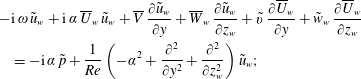 $$\begin{eqnarray}\displaystyle & & \displaystyle \displaystyle -\text{i}\,\unicode[STIX]{x1D714}\,\tilde{u} _{w}+\text{i}\,\unicode[STIX]{x1D6FC}\,\overline{U}_{w}\,\tilde{u} _{w}+\overline{V}\,{\displaystyle \frac{\unicode[STIX]{x2202}\tilde{u} _{w}}{\unicode[STIX]{x2202}y}}+\overline{W}_{w}\,{\displaystyle \frac{\unicode[STIX]{x2202}\tilde{u} _{w}}{\unicode[STIX]{x2202}z_{w}}}+\tilde{v}\,{\displaystyle \frac{\unicode[STIX]{x2202}\overline{U}_{w}}{\unicode[STIX]{x2202}y}}+\tilde{w}_{w}\,{\displaystyle \frac{\unicode[STIX]{x2202}\overline{U}_{w}}{\unicode[STIX]{x2202}z_{w}}}\nonumber\\ \displaystyle & & \displaystyle \quad \displaystyle =-\text{i}\,\unicode[STIX]{x1D6FC}\,\tilde{p}+{\displaystyle \frac{1}{Re}}\left(-\unicode[STIX]{x1D6FC}^{2}+\frac{\unicode[STIX]{x2202}^{2}}{\unicode[STIX]{x2202}y^{2}}+{\displaystyle \frac{\unicode[STIX]{x2202}^{2}}{\unicode[STIX]{x2202}z_{w}^{2}}}\right)\tilde{u} _{w};\end{eqnarray}$$
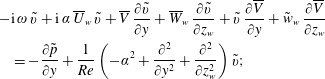 $$\begin{eqnarray}\displaystyle & & \displaystyle \displaystyle -\text{i}\,\unicode[STIX]{x1D714}\,\tilde{v}+\text{i}\,\unicode[STIX]{x1D6FC}\,\overline{U}_{w}\,\tilde{v}+\overline{V}\,\frac{\unicode[STIX]{x2202}\tilde{v}}{\unicode[STIX]{x2202}y}+\overline{W}_{w}\,\frac{\unicode[STIX]{x2202}\tilde{v}}{\unicode[STIX]{x2202}z_{w}}+\tilde{v}\,{\displaystyle \frac{\unicode[STIX]{x2202}\overline{V}}{\unicode[STIX]{x2202}y}}+\tilde{w}_{w}\,{\displaystyle \frac{\unicode[STIX]{x2202}\overline{V}}{\unicode[STIX]{x2202}z_{w}}}\nonumber\\ \displaystyle & & \displaystyle \quad \displaystyle =-{\displaystyle \frac{\unicode[STIX]{x2202}\tilde{p}}{\unicode[STIX]{x2202}y}}+{\displaystyle \frac{1}{Re}}\left(-\unicode[STIX]{x1D6FC}^{2}+{\displaystyle \frac{\unicode[STIX]{x2202}^{2}}{\unicode[STIX]{x2202}y^{2}}}+{\displaystyle \frac{\unicode[STIX]{x2202}^{2}}{\unicode[STIX]{x2202}z_{w}^{2}}}\right)\tilde{v};\end{eqnarray}$$
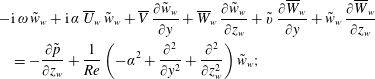 $$\begin{eqnarray}\displaystyle & & \displaystyle \displaystyle -\text{i}\,\unicode[STIX]{x1D714}\,\tilde{w}_{w}+\text{i}\,\unicode[STIX]{x1D6FC}\,\overline{U}_{w}\,\tilde{w}_{w}+\overline{V}\,{\displaystyle \frac{\unicode[STIX]{x2202}\tilde{w}_{w}}{\unicode[STIX]{x2202}y}}+\overline{W}_{w}\,{\displaystyle \frac{\unicode[STIX]{x2202}\tilde{w}_{w}}{\unicode[STIX]{x2202}z_{w}}}+\tilde{v}\,{\displaystyle \frac{\unicode[STIX]{x2202}\overline{W}_{w}}{\unicode[STIX]{x2202}y}}+\tilde{w}_{w}\,{\displaystyle \frac{\unicode[STIX]{x2202}\overline{W}_{w}}{\unicode[STIX]{x2202}z_{w}}}\nonumber\\ \displaystyle & & \displaystyle \quad \displaystyle =-{\displaystyle \frac{\unicode[STIX]{x2202}\tilde{p}}{\unicode[STIX]{x2202}z_{w}}}+{\displaystyle \frac{1}{Re}}\left(-\unicode[STIX]{x1D6FC}^{2}+{\displaystyle \frac{\unicode[STIX]{x2202}^{2}}{\unicode[STIX]{x2202}y^{2}}}+{\displaystyle \frac{\unicode[STIX]{x2202}^{2}}{\unicode[STIX]{x2202}z_{w}^{2}}}\right)\tilde{w}_{w};\end{eqnarray}$$
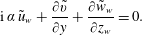 $$\begin{eqnarray}\displaystyle & & \displaystyle \displaystyle \text{i}\,\unicode[STIX]{x1D6FC}\,\tilde{u} _{w}+\frac{\unicode[STIX]{x2202}\tilde{v}}{\unicode[STIX]{x2202}y}+{\displaystyle \frac{\unicode[STIX]{x2202}\tilde{w}_{w}}{\unicode[STIX]{x2202}z_{w}}}=0.\end{eqnarray}$$
 $z_{w}y$
-plane. The in-plane base flow velocity components
$z_{w}y$
-plane. The in-plane base flow velocity components
 $\overline{V}$
and
$\overline{V}$
and
 $\overline{W}_{w}$
appear amongst the coefficients in the equations, illustrating their role as advection and reaction terms. The
$\overline{W}_{w}$
appear amongst the coefficients in the equations, illustrating their role as advection and reaction terms. The
 $\overline{V}$
-terms are no longer absent, as in the one-dimensional Orr-Sommerfeld analyses due to the parallel flow assumption. In two-dimensional approaches, this assumption is lifted, because of flow continuity in the plane. Therefore all velocity components are required as part of the measurement data to complete the general eigenmode description.
$\overline{V}$
-terms are no longer absent, as in the one-dimensional Orr-Sommerfeld analyses due to the parallel flow assumption. In two-dimensional approaches, this assumption is lifted, because of flow continuity in the plane. Therefore all velocity components are required as part of the measurement data to complete the general eigenmode description. Together with the aforementioned boundary conditions, the system (3.2) is solved for
 $\unicode[STIX]{x1D714}\in \mathbb{C}$
(given
$\unicode[STIX]{x1D714}\in \mathbb{C}$
(given
 $\unicode[STIX]{x1D6FC}\in \mathbb{R}$
) or
$\unicode[STIX]{x1D6FC}\in \mathbb{R}$
) or
 $\unicode[STIX]{x1D6FC}\in \mathbb{C}$
(given
$\unicode[STIX]{x1D6FC}\in \mathbb{C}$
(given
 $\unicode[STIX]{x1D714}\in \mathbb{R}$
), in what is called the temporal or spatial framework, respectively. In the considered experimental framework, the secondary perturbations of interest are convective; i.e. they grow as they travel in the downstream direction, while having constant amplitude at a fixed point in space, see Wassermann & Kloker (Reference Wassermann and Kloker2002) and Serpieri & Kotsonis (Reference Serpieri and Kotsonis2016). This corresponds to the spatial stability framework. The spatial stability problem is a quadratic eigenvalue problem, which is computationally more expensive to solve than the temporal problem. Previous work indicates that the Gaster transformation can be successfully applied to link the spatial and temporal solutions, see Malik et al. (Reference Malik, Li and Chang1994, Reference Malik, Li, Choudhari and Chang1999) and Koch et al. (Reference Koch, Bertolotti, Stolte and Hein2000). The majority of the eigensolutions presented here are hence based on the temporal approach, applying the Gaster transformation when in need of the spatial characteristics. The validity of the Gaster transformation is verified in § 4.5, where the spatial problem is solved, i.e.
$\unicode[STIX]{x1D714}\in \mathbb{R}$
), in what is called the temporal or spatial framework, respectively. In the considered experimental framework, the secondary perturbations of interest are convective; i.e. they grow as they travel in the downstream direction, while having constant amplitude at a fixed point in space, see Wassermann & Kloker (Reference Wassermann and Kloker2002) and Serpieri & Kotsonis (Reference Serpieri and Kotsonis2016). This corresponds to the spatial stability framework. The spatial stability problem is a quadratic eigenvalue problem, which is computationally more expensive to solve than the temporal problem. Previous work indicates that the Gaster transformation can be successfully applied to link the spatial and temporal solutions, see Malik et al. (Reference Malik, Li and Chang1994, Reference Malik, Li, Choudhari and Chang1999) and Koch et al. (Reference Koch, Bertolotti, Stolte and Hein2000). The majority of the eigensolutions presented here are hence based on the temporal approach, applying the Gaster transformation when in need of the spatial characteristics. The validity of the Gaster transformation is verified in § 4.5, where the spatial problem is solved, i.e.
 $\unicode[STIX]{x1D6FC}\in \mathbb{C}$
is unknown and
$\unicode[STIX]{x1D6FC}\in \mathbb{C}$
is unknown and
 $\unicode[STIX]{x1D714}\in \mathbb{R}$
is given.
$\unicode[STIX]{x1D714}\in \mathbb{R}$
is given.
In what follows, our main interest is in the most unstable eigensolutions and the solution that can be compared to the relevant POD mode obtained from the tomo-PIV data. In the latter case, the quantity directly measured from POD is the wavelength of the type I mode, which equals
 $4.6~\text{mm}$
. Hence solutions are sought for which
$4.6~\text{mm}$
. Hence solutions are sought for which
 $2\unicode[STIX]{x03C0}/\unicode[STIX]{x1D6FC}_{r}=4.6~\text{mm}$
.
$2\unicode[STIX]{x03C0}/\unicode[STIX]{x1D6FC}_{r}=4.6~\text{mm}$
.
3.2 Reynolds–Orr equation
To cast the eigenmodes in a more physically interpretable form, the eigenvalues are decomposed into the values attributed to specific terms in the governing system of equations. To this end, the dot product of the system of equations (taking the complex conjugate of the continuity equation) with the variable vector
 $[\tilde{u} _{w}^{\ast }\,\tilde{v}^{\ast }\,\tilde{w}_{w}^{\ast }\,\tilde{p}]^{\text{T}}$
is used and integrated over both spanwise and wall-normal directions (executing the proper function inner product). Integrating the continuity equation and viscous terms by parts and solving for
$[\tilde{u} _{w}^{\ast }\,\tilde{v}^{\ast }\,\tilde{w}_{w}^{\ast }\,\tilde{p}]^{\text{T}}$
is used and integrated over both spanwise and wall-normal directions (executing the proper function inner product). Integrating the continuity equation and viscous terms by parts and solving for
 $\unicode[STIX]{x1D714}$
yields:
$\unicode[STIX]{x1D714}$
yields:
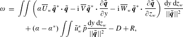 $$\begin{eqnarray}\displaystyle \unicode[STIX]{x1D714} & = & \displaystyle \iint \left(\unicode[STIX]{x1D6FC}\overline{U}_{w}\,\tilde{\boldsymbol{q}}^{\ast }\boldsymbol{\cdot }\tilde{\boldsymbol{q}}-\text{i}\,\overline{V}\,\tilde{\boldsymbol{q}}^{\ast }\boldsymbol{\cdot }{\displaystyle \frac{\unicode[STIX]{x2202}\tilde{\boldsymbol{q}}}{\unicode[STIX]{x2202}y}}-\text{i}\,\overline{W}_{w}\,\tilde{\boldsymbol{q}}^{\ast }\boldsymbol{\cdot }\frac{\unicode[STIX]{x2202}\tilde{\boldsymbol{q}}}{\unicode[STIX]{x2202}z_{w}}\right){\displaystyle \frac{\text{d}y\,\text{d}z_{w}}{||\tilde{\boldsymbol{q}}||^{2}}}\nonumber\\ \displaystyle & & \displaystyle \quad +\,(\unicode[STIX]{x1D6FC}-\unicode[STIX]{x1D6FC}^{\ast })\iint \tilde{u} _{w}^{\ast }\hspace{2.0pt}\tilde{p}{\displaystyle \frac{\text{d}y\,\text{d}z_{w}}{||\tilde{\boldsymbol{q}}||^{2}}}-D+R,\end{eqnarray}$$
where
 $\tilde{\boldsymbol{q}}=[\tilde{u} _{w}\,\tilde{v}\,\tilde{w}_{w}]^{\text{T}}$
and
$\tilde{\boldsymbol{q}}=[\tilde{u} _{w}\,\tilde{v}\,\tilde{w}_{w}]^{\text{T}}$
and
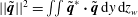 $||\tilde{\boldsymbol{q}}||^{2}=\iint \tilde{\boldsymbol{q}}^{\ast }\boldsymbol{\cdot }\tilde{\boldsymbol{q}}\;\text{d}y\,\text{d}z_{w}$
. From left to right, the terms represent advection, pressure work (zero when
$||\tilde{\boldsymbol{q}}||^{2}=\iint \tilde{\boldsymbol{q}}^{\ast }\boldsymbol{\cdot }\tilde{\boldsymbol{q}}\;\text{d}y\,\text{d}z_{w}$
. From left to right, the terms represent advection, pressure work (zero when
 $\unicode[STIX]{x1D6FC}_{i}=0$
), viscous dissipation
$\unicode[STIX]{x1D6FC}_{i}=0$
), viscous dissipation
 $D$
and Reynolds stress work
$D$
and Reynolds stress work
 $R$
. The latter two terms represent the combinations of terms:
$R$
. The latter two terms represent the combinations of terms:
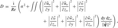 $$\begin{eqnarray}\displaystyle \displaystyle D & = & \displaystyle {\displaystyle \frac{\text{i}}{Re}}\left(\unicode[STIX]{x1D6FC}^{2}+\iint \left(\left|{\displaystyle \frac{\unicode[STIX]{x2202}\tilde{u} _{w}}{\unicode[STIX]{x2202}y}}\right|^{2}+\left|{\displaystyle \frac{\unicode[STIX]{x2202}\tilde{u} _{w}}{\unicode[STIX]{x2202}z_{w}}}\right|^{2}+\left|{\displaystyle \frac{\unicode[STIX]{x2202}\tilde{v}}{\unicode[STIX]{x2202}y}}\right|^{2}\right.\right.\nonumber\\ \displaystyle & & \displaystyle \quad \left.\left.+\,\left|{\displaystyle \frac{\unicode[STIX]{x2202}\tilde{v}}{\unicode[STIX]{x2202}z_{w}}}\right|^{2}+\left|{\displaystyle \frac{\unicode[STIX]{x2202}\tilde{w}_{w}}{\unicode[STIX]{x2202}y}}\right|^{2}+\left|{\displaystyle \frac{\unicode[STIX]{x2202}\tilde{w}_{w}}{\unicode[STIX]{x2202}z_{w}}}\right|^{2}\right){\displaystyle \frac{\text{d}y\,\text{d}z_{w}}{||\tilde{\boldsymbol{q}}||^{2}}}\right),\end{eqnarray}$$
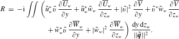 $$\begin{eqnarray}\displaystyle R & = & \displaystyle -\text{i}\iint \left(\tilde{u} _{w}^{\ast }\tilde{v}\;{\displaystyle \frac{\unicode[STIX]{x2202}\overline{U}_{w}}{\unicode[STIX]{x2202}y}}+\tilde{u} _{w}^{\ast }\tilde{w}_{w}\;{\displaystyle \frac{\unicode[STIX]{x2202}\overline{U}_{w}}{\unicode[STIX]{x2202}z_{w}}}+|\tilde{v}|^{2}\;{\displaystyle \frac{\unicode[STIX]{x2202}\overline{V}}{\unicode[STIX]{x2202}y}}+\tilde{v}^{\ast }\tilde{w}_{w}\;{\displaystyle \frac{\unicode[STIX]{x2202}\overline{V}}{\unicode[STIX]{x2202}z_{w}}}\right.\nonumber\\ \displaystyle & & \displaystyle \quad \left.+\,\tilde{w}_{w}^{\ast }\tilde{v}\;{\displaystyle \frac{\unicode[STIX]{x2202}\overline{W}_{w}}{\unicode[STIX]{x2202}y}}+|\tilde{w}_{w}|^{2}\;{\displaystyle \frac{\unicode[STIX]{x2202}\overline{W}_{w}}{\unicode[STIX]{x2202}z_{w}}}\right){\displaystyle \frac{\text{d}y\,\text{d}z_{w}}{||\tilde{\boldsymbol{q}}||^{2}}}.\end{eqnarray}$$
Equation (3.3) is referred to as the Reynolds–Orr equation, see Schmid & Henningson (Reference Schmid and Henningson2001). Note that due to the particular periodic and no-slip boundary conditions on the amplitude functions considered in this case, no boundary terms appear. The different terms of (3.3) represent the complex contribution to
 $\unicode[STIX]{x1D714}$
associated with specific physical mechanisms pertinent to the base flow. Usually, the equation is used in the Lagrangian form that excludes the advection terms, see Malik et al. (Reference Malik, Li and Chang1996) and Schmid & Henningson (Reference Schmid and Henningson2001), here these terms do appear as the Eulerian form is considered.
$\unicode[STIX]{x1D714}$
associated with specific physical mechanisms pertinent to the base flow. Usually, the equation is used in the Lagrangian form that excludes the advection terms, see Malik et al. (Reference Malik, Li and Chang1996) and Schmid & Henningson (Reference Schmid and Henningson2001), here these terms do appear as the Eulerian form is considered.
The following shorthand symbols are introduced for ease of reference:
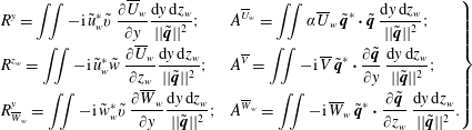 $$\begin{eqnarray}\displaystyle \left.\begin{array}{@{}ll@{}}\displaystyle R^{y}=\iint -\text{i}\,\tilde{u} _{w}^{\ast }\tilde{v}\;{\displaystyle \frac{\unicode[STIX]{x2202}\overline{U}_{w}}{\unicode[STIX]{x2202}y}}{\displaystyle \frac{\text{d}y\,\text{d}z_{w}}{||\tilde{\boldsymbol{q}}||^{2}}}; & \displaystyle A^{\overline{U}_{w}}=\iint \unicode[STIX]{x1D6FC}\overline{U}_{w}\,\tilde{\boldsymbol{q}}^{\ast }\boldsymbol{\cdot }\tilde{\boldsymbol{q}}\;{\displaystyle \frac{\text{d}y\,\text{d}z_{w}}{||\tilde{\boldsymbol{q}}||^{2}}};\\[9.0pt] \displaystyle R^{z_{w}}=\iint -\text{i}\,\tilde{u} _{w}^{\ast }\tilde{w}\;{\displaystyle \frac{\unicode[STIX]{x2202}\overline{U}_{w}}{\unicode[STIX]{x2202}z_{w}}}{\displaystyle \frac{\text{d}y\,\text{d}z_{w}}{||\tilde{\boldsymbol{q}}||^{2}}}; & \displaystyle A^{\overline{V}}=\iint -\text{i}\,\overline{V}\,\tilde{\boldsymbol{q}}^{\ast }\boldsymbol{\cdot }{\displaystyle \frac{\unicode[STIX]{x2202}\tilde{\boldsymbol{q}}}{\unicode[STIX]{x2202}y}}\;{\displaystyle \frac{\text{d}y\,\text{d}z_{w}}{||\tilde{\boldsymbol{q}}||^{2}}};\\[9.0pt] \displaystyle R_{\overline{W}_{w}}^{y}=\iint -\text{i}\,\tilde{w}_{w}^{\ast }\tilde{v}\;{\displaystyle \frac{\unicode[STIX]{x2202}\overline{W}_{w}}{\unicode[STIX]{x2202}y}}{\displaystyle \frac{\text{d}y\,\text{d}z_{w}}{||\tilde{\boldsymbol{q}}||^{2}}}; & A^{\overline{W}_{w}}=\displaystyle \iint -\text{i}\,\overline{W}_{w}\,\tilde{\boldsymbol{q}}^{\ast }\boldsymbol{\cdot }{\displaystyle \frac{\unicode[STIX]{x2202}\tilde{\boldsymbol{q}}}{\unicode[STIX]{x2202}z_{w}}}\;\displaystyle {\displaystyle \frac{\text{d}y\,\text{d}z_{w}}{||\tilde{\boldsymbol{q}}||^{2}}}.\end{array}\right\} & & \displaystyle\end{eqnarray}$$
Whenever a reference is made to the integrands of the above terms, the inclusion of the scaling factor
 $||\tilde{\boldsymbol{q}}||^{2}$
is implied.
$||\tilde{\boldsymbol{q}}||^{2}$
is implied.
By substituting the eigensolutions, each term on the right-hand side of (3.3) can be numerically evaluated. The advection terms generally have a large real part and thus dominate the real part of
 $\unicode[STIX]{x1D714}$
; i.e. the
$\unicode[STIX]{x1D714}$
; i.e. the
 $\unicode[STIX]{x1D714}_{r}$
-budget. The Reynolds stresses and viscous dissipation have a larger imaginary part and therefore determine the growth rate, i.e. the
$\unicode[STIX]{x1D714}_{r}$
-budget. The Reynolds stresses and viscous dissipation have a larger imaginary part and therefore determine the growth rate, i.e. the
 $\unicode[STIX]{x1D714}_{i}$
-budget, which is a measure of the production or destruction of the perturbation energy. All terms that do not involve the absolute magnitude of an amplitude function are generally complex. Thus the advection terms and Reynolds (shear) stresses do generally contribute respectively to the
$\unicode[STIX]{x1D714}_{i}$
-budget, which is a measure of the production or destruction of the perturbation energy. All terms that do not involve the absolute magnitude of an amplitude function are generally complex. Thus the advection terms and Reynolds (shear) stresses do generally contribute respectively to the
 $\unicode[STIX]{x1D714}_{i}$
- and
$\unicode[STIX]{x1D714}_{i}$
- and
 $\unicode[STIX]{x1D714}_{r}$
-budgets as well, albeit to a minor extent.
$\unicode[STIX]{x1D714}_{r}$
-budgets as well, albeit to a minor extent.
The individual terms in the
 $\unicode[STIX]{x1D714}_{r}$
- and
$\unicode[STIX]{x1D714}_{r}$
- and
 $\unicode[STIX]{x1D714}_{i}$
-budgets encode the underlying physical mechanisms of every eigenmode; defining their very nature. This work focuses on the consistency of those terms for each eigenmode, for example that the terms show the same magnitude independent of the ensemble size
$\unicode[STIX]{x1D714}_{i}$
-budgets encode the underlying physical mechanisms of every eigenmode; defining their very nature. This work focuses on the consistency of those terms for each eigenmode, for example that the terms show the same magnitude independent of the ensemble size
 $N_{fr}$
. In particular those terms involving the (difficult to measure)
$N_{fr}$
. In particular those terms involving the (difficult to measure)
 $\overline{V}$
and
$\overline{V}$
and
 $\overline{W}_{w}$
deserve emphasis, due to the sensitivity of the stability outcomes to those terms, as discussed by Bonfigli & Kloker (Reference Bonfigli and Kloker2007).
$\overline{W}_{w}$
deserve emphasis, due to the sensitivity of the stability outcomes to those terms, as discussed by Bonfigli & Kloker (Reference Bonfigli and Kloker2007).
A general criterion can be derived that indicates a local destabilizing contribution due to advection. The advection terms in the
 $\unicode[STIX]{x1D714}_{i}$
-budget can be written as:
$\unicode[STIX]{x1D714}_{i}$
-budget can be written as:
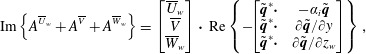 $$\begin{eqnarray}\displaystyle \text{Im}\left\{A^{\overline{U}_{w}}+A^{\overline{V}}+A^{\overline{W}_{w}}\right\}=\left[\begin{array}{@{}c@{}}\overline{U}_{w}\\ \overline{V}\\ \overline{W}_{w}\end{array}\right]\boldsymbol{\cdot }\;\text{Re}\left\{-\!\!\left[\begin{array}{@{}cc@{}}\tilde{\boldsymbol{q}}^{\ast }\boldsymbol{\cdot } & -\unicode[STIX]{x1D6FC}_{i}\tilde{\boldsymbol{q}}\\ \tilde{\boldsymbol{q}}^{\ast }\boldsymbol{\cdot } & \unicode[STIX]{x2202}\tilde{\boldsymbol{q}}/\unicode[STIX]{x2202}y\\ \tilde{\boldsymbol{q}}^{\ast }\boldsymbol{\cdot } & \unicode[STIX]{x2202}\tilde{\boldsymbol{q}}/\unicode[STIX]{x2202}z_{w}\end{array}\right]\right\}, & & \displaystyle\end{eqnarray}$$
(where
 $\text{Re}$
, not in italics, denotes the real part) which is (non-)zero whenever the perturbation amplitude gradient is (non-)orthogonal to the in-plane flow. Bonfigli & Kloker (Reference Bonfigli and Kloker2007) argue that a velocity component normal to the shear layer moves the perturbations away from the productive region and hence has a stabilizing effect. However, the former criterion illustrates the opposite and is therefore object of dedicated analysis in the remainder. Whenever the velocity vector is aligned with the direction in which the perturbation decays, this results in a locally destabilizing effect. I.e. a region of high perturbation energy is moved so as to replace a lower energy region. On the other hand, if the perturbation grows in the advection direction, that is stabilizing. Generally, advection is destabilizing if it is effective in transferring energy to the exterior of the vortex core.
$\text{Re}$
, not in italics, denotes the real part) which is (non-)zero whenever the perturbation amplitude gradient is (non-)orthogonal to the in-plane flow. Bonfigli & Kloker (Reference Bonfigli and Kloker2007) argue that a velocity component normal to the shear layer moves the perturbations away from the productive region and hence has a stabilizing effect. However, the former criterion illustrates the opposite and is therefore object of dedicated analysis in the remainder. Whenever the velocity vector is aligned with the direction in which the perturbation decays, this results in a locally destabilizing effect. I.e. a region of high perturbation energy is moved so as to replace a lower energy region. On the other hand, if the perturbation grows in the advection direction, that is stabilizing. Generally, advection is destabilizing if it is effective in transferring energy to the exterior of the vortex core.
3.3 Discretization
The BiGlobal tools of the VKI extensible stability and transition analysis (VESTA) toolkit are used to set up the stability problem, see Pinna (Reference Pinna2012). The problem is discretized using Chebyshev spectral collocation combined with a biquadratic mapping resolving both
 $y$
- and
$y$
- and
 $z_{w}$
-directions in specific areas. It should be noted that an alternative to this discretization involves Floquet theory; solving the Fourier transformed problem in the spanwise direction, see Herbert (Reference Herbert1988), Janke & Balakumar (Reference Janke and Balakumar2000) and Koch et al. (Reference Koch, Bertolotti, Stolte and Hein2000). Theofilis (Reference Theofilis2003) notes that a large number of Fourier coefficients has to be resolved and hence the method is not necessarily cheaper than solving the partial differential problem directly.
$z_{w}$
-directions in specific areas. It should be noted that an alternative to this discretization involves Floquet theory; solving the Fourier transformed problem in the spanwise direction, see Herbert (Reference Herbert1988), Janke & Balakumar (Reference Janke and Balakumar2000) and Koch et al. (Reference Koch, Bertolotti, Stolte and Hein2000). Theofilis (Reference Theofilis2003) notes that a large number of Fourier coefficients has to be resolved and hence the method is not necessarily cheaper than solving the partial differential problem directly.
The biquadratic mapping is defined in terms of the
 $y$
-coordinate as follows:
$y$
-coordinate as follows:
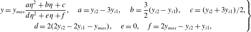 $$\begin{eqnarray}\displaystyle \hspace{-18.0pt}\left.\begin{array}{@{}c@{}}\displaystyle y=y_{max}{\displaystyle \frac{a\unicode[STIX]{x1D702}^{2}+b\unicode[STIX]{x1D702}+c}{d\unicode[STIX]{x1D702}^{2}+e\unicode[STIX]{x1D702}+f}},\quad a=y_{i2}-3y_{i1},\quad b=\frac{3}{2}(y_{i2}-y_{i1}),\quad c=(y_{i2}+3y_{i1})/2,\\ \displaystyle d=2(2y_{i2}-2y_{i1}-y_{max}),\quad e=0,\quad f=2y_{max}-y_{i2}+y_{i1},\end{array}\right\} & & \displaystyle\end{eqnarray}$$
where
 $\unicode[STIX]{x1D702}$
represents the Chebyshev Gauss–Lobatto quadrature points spanning the range
$\unicode[STIX]{x1D702}$
represents the Chebyshev Gauss–Lobatto quadrature points spanning the range
 $[-1,1]$
, see Canuto et al. (Reference Canuto, Hussaini, Quarteroni and Zang2006), and
$[-1,1]$
, see Canuto et al. (Reference Canuto, Hussaini, Quarteroni and Zang2006), and
 $y$
the node coordinates in physical space spanning
$y$
the node coordinates in physical space spanning
 $[0,y_{max}]$
. The mapping is conceived as a generalization to that used by Malik (Reference Malik1990), set so as to distribute one third of the collocation nodes over the domains
$[0,y_{max}]$
. The mapping is conceived as a generalization to that used by Malik (Reference Malik1990), set so as to distribute one third of the collocation nodes over the domains
 $[0,y_{i1}]$
,
$[0,y_{i1}]$
,
 $[y_{i1},y_{i2}]$
and
$[y_{i1},y_{i2}]$
and
 $[y_{i2},y_{max}]$
, as long as
$[y_{i2},y_{max}]$
, as long as
 $0<y_{i1}<y_{i2}<y_{max}$
and
$0<y_{i1}<y_{i2}<y_{max}$
and
 $y_{i2}<9y_{i1}$
and
$y_{i2}<9y_{i1}$
and
 $9y_{i2}<y_{i1}+8y_{max}$
to ensure a regular monotonic behaviour without discontinuities. The resulting grids maintain a cosine distribution near the boundaries. The same mapped Chebyshev collocation discretization is applied in the
$9y_{i2}<y_{i1}+8y_{max}$
to ensure a regular monotonic behaviour without discontinuities. The resulting grids maintain a cosine distribution near the boundaries. The same mapped Chebyshev collocation discretization is applied in the
 $z_{w}$
-direction. As opposed to the commonly used Floquet approach, this allows the specification of arbitrary, i.e. non-periodic, flow fields. Although periodic boundary conditions are applied at the boundaries in the spanwise direction, periodizing the base flow fields is avoided in the present study, to circumvent introducing artificial shear layers. This is a posteriori justified, as will be shown in § 4.8.
$z_{w}$
-direction. As opposed to the commonly used Floquet approach, this allows the specification of arbitrary, i.e. non-periodic, flow fields. Although periodic boundary conditions are applied at the boundaries in the spanwise direction, periodizing the base flow fields is avoided in the present study, to circumvent introducing artificial shear layers. This is a posteriori justified, as will be shown in § 4.8.
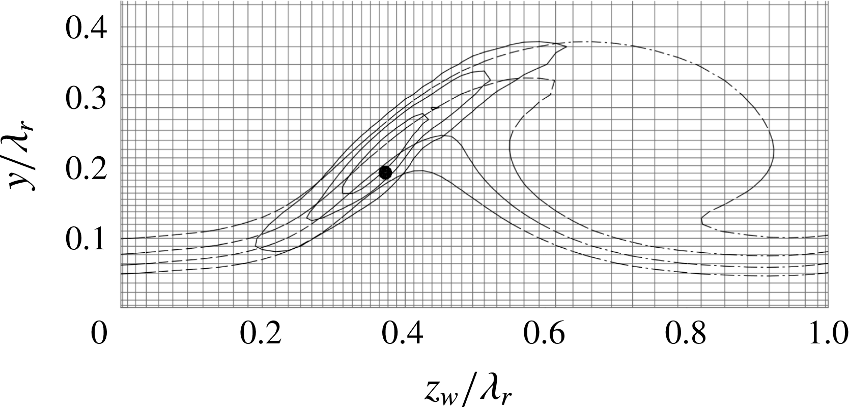
Figure 6. Zoom of mapped Chebyshev grid (
 $55\times 55$
nodes).
$55\times 55$
nodes).
 $|\tilde{u} _{w}|/\max |\tilde{u} _{w}|$
of type I (solid contours at 25 %, 50 % and 75 %).
$|\tilde{u} _{w}|/\max |\tilde{u} _{w}|$
of type I (solid contours at 25 %, 50 % and 75 %).
 $\overline{U}_{w}/\overline{U}_{e}$
levels 0.6, 0.7, 0.8 and 0.9 (dash-dotted). Position of
$\overline{U}_{w}/\overline{U}_{e}$
levels 0.6, 0.7, 0.8 and 0.9 (dash-dotted). Position of
 $(\overline{V},\overline{W}_{w})$
-field saddle point (solid circle).
$(\overline{V},\overline{W}_{w})$
-field saddle point (solid circle).
When considering a domain with a single vortex, the mapping is equipped with specific parameters aimed at densely resolving the region where the type I eigenfunction is located, about the saddle point of the in-plane flow. Using
 $N_{z}\times N_{y}=55\times 55$
nodes and setting
$N_{z}\times N_{y}=55\times 55$
nodes and setting
 $(z_{i1},z_{i2},z_{max})=(0.30;0.55;1.0)\unicode[STIX]{x1D706}_{r}$
and
$(z_{i1},z_{i2},z_{max})=(0.30;0.55;1.0)\unicode[STIX]{x1D706}_{r}$
and
 $(y_{i1},y_{i2},y_{max})=(0.18;0.60;4.0)\unicode[STIX]{x1D706}_{r}$
yields type I eigenvalue errors of
$(y_{i1},y_{i2},y_{max})=(0.18;0.60;4.0)\unicode[STIX]{x1D706}_{r}$
yields type I eigenvalue errors of
 $O(10^{-5})$
in the absolute value of the real and imaginary parts, separately. An example of the spatial distribution of mode I on the grid is shown in figure 6. Grid convergence was verified by increasing the resolution using these mapping parameters and checking against more conventional grids, applying no or the standard bilinear mapping of Malik (Reference Malik1990). The type II modes, positioned about the point
$O(10^{-5})$
in the absolute value of the real and imaginary parts, separately. An example of the spatial distribution of mode I on the grid is shown in figure 6. Grid convergence was verified by increasing the resolution using these mapping parameters and checking against more conventional grids, applying no or the standard bilinear mapping of Malik (Reference Malik1990). The type II modes, positioned about the point
 $(z_{w},y)/\unicode[STIX]{x1D706}_{r}=(0.7,0.35)$
that is relatively sparsely covered with nodes, has yet to overcome larger eigenvalue differences with higher resolution results. Nevertheless, the real and imaginary parts of the eigenvalue corresponding to the most unstable type II mode undergo
$(z_{w},y)/\unicode[STIX]{x1D706}_{r}=(0.7,0.35)$
that is relatively sparsely covered with nodes, has yet to overcome larger eigenvalue differences with higher resolution results. Nevertheless, the real and imaginary parts of the eigenvalue corresponding to the most unstable type II mode undergo
 $O(10^{-4})$
absolute changes when changing the grid size from
$O(10^{-4})$
absolute changes when changing the grid size from
 $55\times 55$
to
$55\times 55$
to
 $90\times 90$
, which is deemed sufficiently small for the current purposes.
$90\times 90$
, which is deemed sufficiently small for the current purposes.
In the case of the domain with both vortices, i.e.
 $z_{w}/\unicode[STIX]{x1D706}_{r}\in [-1,1]$
, the mapping was programmed to distribute the collocation nodes as uniformly as possible, corresponding to
$z_{w}/\unicode[STIX]{x1D706}_{r}\in [-1,1]$
, the mapping was programmed to distribute the collocation nodes as uniformly as possible, corresponding to
 $(z_{i1},z_{i2},z_{max})=(-1/3,1/3,1)\unicode[STIX]{x1D706}_{r}$
. The discretization in the
$(z_{i1},z_{i2},z_{max})=(-1/3,1/3,1)\unicode[STIX]{x1D706}_{r}$
. The discretization in the
 $y$
-direction is left unchanged.
$y$
-direction is left unchanged.
The column-stacked representation of the eigenfunctions as elaborated upon by Groot (Reference Groot2013) is used, which casts the system (3.2) into one of the following forms:
 $$\begin{eqnarray}\displaystyle & \displaystyle \text{temporal:}\quad \unicode[STIX]{x1D63C}_{\unicode[STIX]{x1D714}}\tilde{\boldsymbol{V}}_{\unicode[STIX]{x1D714}}=\unicode[STIX]{x1D714}\unicode[STIX]{x1D63D}_{\unicode[STIX]{x1D714}}\tilde{\boldsymbol{V}}_{\unicode[STIX]{x1D714}}; & \displaystyle\end{eqnarray}$$
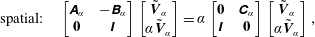 $$\begin{eqnarray}\displaystyle & \displaystyle \text{spatial:}\quad \left[\begin{array}{@{}cc@{}}\unicode[STIX]{x1D63C}_{\unicode[STIX]{x1D6FC}} & -\unicode[STIX]{x1D63D}_{\unicode[STIX]{x1D6FC}}\\ \text{}\text{0} & \unicode[STIX]{x1D644}\end{array}\right]\left[\begin{array}{@{}c@{}}\tilde{\boldsymbol{V}}_{\unicode[STIX]{x1D6FC}}\\ \unicode[STIX]{x1D6FC}\tilde{\boldsymbol{V}}_{\unicode[STIX]{x1D6FC}}\end{array}\right]=\unicode[STIX]{x1D6FC}\left[\begin{array}{@{}cc@{}}\text{}\text{0} & \unicode[STIX]{x1D63E}_{\unicode[STIX]{x1D6FC}}\\ \unicode[STIX]{x1D644} & \mathbf{0}\end{array}\right]\left[\begin{array}{@{}c@{}}\tilde{\boldsymbol{V}}_{\unicode[STIX]{x1D6FC}}\\ \unicode[STIX]{x1D6FC}\tilde{\boldsymbol{V}}_{\unicode[STIX]{x1D6FC}}\end{array}\right], & \displaystyle\end{eqnarray}$$
where
 $\tilde{\boldsymbol{V}}=[\tilde{u} _{w}\,\tilde{v}\,\tilde{w}_{w}\,\tilde{p}]^{\text{T}}$
, the matrices
$\tilde{\boldsymbol{V}}=[\tilde{u} _{w}\,\tilde{v}\,\tilde{w}_{w}\,\tilde{p}]^{\text{T}}$
, the matrices
 $\unicode[STIX]{x1D63C}$
,
$\unicode[STIX]{x1D63C}$
,
 $\unicode[STIX]{x1D63D}$
and
$\unicode[STIX]{x1D63D}$
and
 $\unicode[STIX]{x1D63E}$
contain the coefficients of system (3.2) that multiply the eigenvalue to the zeroth, first and second powers, respectively, and the matrices
$\unicode[STIX]{x1D63E}$
contain the coefficients of system (3.2) that multiply the eigenvalue to the zeroth, first and second powers, respectively, and the matrices
 $\mathbf{0}$
and
$\mathbf{0}$
and
 $\unicode[STIX]{x1D644}$
represent the zero and identity matrices with the same size as
$\unicode[STIX]{x1D644}$
represent the zero and identity matrices with the same size as
 $\unicode[STIX]{x1D63C}$
. Equation (3.10) represents the companion matrix approach, casting the spatial problem into a (twice as large) regular eigenvalue problem, see Schmid & Henningson (Reference Schmid and Henningson2001).
$\unicode[STIX]{x1D63C}$
. Equation (3.10) represents the companion matrix approach, casting the spatial problem into a (twice as large) regular eigenvalue problem, see Schmid & Henningson (Reference Schmid and Henningson2001).
Using the biquadratic mapping markedly reduces the computational expenses, in terms of memory and evaluation time. The achieved reduction in the necessary amount of nodes rendered both temporal and spatial problems small enough to be solved on a standard workstation in mass.
3.4 Shift-invert strategy
A final step towards improving solving efficiency is setting the centre of the resolved spectrum; i.e. adjusting the parameters for the shift & invert transformation in the Arnoldi algorithm, see Theofilis (Reference Theofilis2003). This is done considering specific heuristics: the maxima of the eigenfunctions of interest are all positioned high in the boundary layer, away from the near-wall region indicated in figure 2. Conversely, the modes that lie inside the near-wall region are expected to be subject to errors associated with measurement noise. Modes that lie in the near-wall region have low phase speeds corresponding to the low
 $\overline{U}_{w}$
values, by inspection smaller than
$\overline{U}_{w}$
values, by inspection smaller than
 $0.4\overline{U}_{e}$
. Hence, the region with
$0.4\overline{U}_{e}$
. Hence, the region with
 $\unicode[STIX]{x1D714}_{r}<0.4\unicode[STIX]{x1D6FC}_{r}$
, especially the stable region, is avoided. Figure 7 illustrates examples of temporal spectra for
$\unicode[STIX]{x1D714}_{r}<0.4\unicode[STIX]{x1D6FC}_{r}$
, especially the stable region, is avoided. Figure 7 illustrates examples of temporal spectra for
 $\unicode[STIX]{x1D6FC}\unicode[STIX]{x1D706}_{r}=1.0$
and 8.2. The limit
$\unicode[STIX]{x1D6FC}\unicode[STIX]{x1D706}_{r}=1.0$
and 8.2. The limit
 $\unicode[STIX]{x1D714}_{r}=0.4\unicode[STIX]{x1D6FC}_{r}$
is indicated by the dash-dotted line.
$\unicode[STIX]{x1D714}_{r}=0.4\unicode[STIX]{x1D6FC}_{r}$
is indicated by the dash-dotted line.
Figure 7. Resolved spectra using
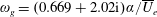 $\unicode[STIX]{x1D714}_{g}=(0.669+2.02\text{i})\unicode[STIX]{x1D6FC}/\overline{U}_{e}$
, corresponding to
$\unicode[STIX]{x1D714}_{g}=(0.669+2.02\text{i})\unicode[STIX]{x1D6FC}/\overline{U}_{e}$
, corresponding to
 $\unicode[STIX]{x1D6FC}\unicode[STIX]{x1D706}_{r}=$
1.0 (a) and
$\unicode[STIX]{x1D6FC}\unicode[STIX]{x1D706}_{r}=$
1.0 (a) and
 $8.2$
(b). Continuous spectrum (solid surface). Modes dominant in the near-wall region (left of dash-dotted line).
$8.2$
(b). Continuous spectrum (solid surface). Modes dominant in the near-wall region (left of dash-dotted line).
 $\unicode[STIX]{x1D714}_{g}$
-centred circle enclosing resolved eigenvalues (dashed line).
$\unicode[STIX]{x1D714}_{g}$
-centred circle enclosing resolved eigenvalues (dashed line).
Additionally, the modes of interest are discrete and do not belong to the continuous spectrum. The continuous spectrum contains modes that live in the free stream and have phase velocity equal to 1, accounting for
 $\overline{W}_{w}$
. They complete the spectrum, but are very expensive to compute in terms of computational time. Due to
$\overline{W}_{w}$
. They complete the spectrum, but are very expensive to compute in terms of computational time. Due to
 $\overline{W}_{w,e}$
being non-zero, the upper bound of the spectrum in the
$\overline{W}_{w,e}$
being non-zero, the upper bound of the spectrum in the
 $\unicode[STIX]{x1D714}$
-plane is the parabola shown in figure 7, with its vertex at
$\unicode[STIX]{x1D714}$
-plane is the parabola shown in figure 7, with its vertex at
 $\unicode[STIX]{x1D6FC}(1-\text{i}\unicode[STIX]{x1D6FC}/Re)$
. The shift
$\unicode[STIX]{x1D6FC}(1-\text{i}\unicode[STIX]{x1D6FC}/Re)$
. The shift
 $\unicode[STIX]{x1D714}_{g}=(0.669+2.02\text{i})\unicode[STIX]{x1D6FC}/\overline{U}_{e}$
is oriented such as to equally avoid both (stable) near-wall and continuous spectrum regions, but to capture all interesting discrete modes. See Wheeler & Barkley (Reference Wheeler and Barkley2006) for a similar approach.
$\unicode[STIX]{x1D714}_{g}=(0.669+2.02\text{i})\unicode[STIX]{x1D6FC}/\overline{U}_{e}$
is oriented such as to equally avoid both (stable) near-wall and continuous spectrum regions, but to capture all interesting discrete modes. See Wheeler & Barkley (Reference Wheeler and Barkley2006) for a similar approach.
As only the modes of interest are captured and the type I mode is usually most unstable, it suffices to reduce the number of resolved modes to 5, which significantly reduces the required time to obtain individual spectra. Note that the imaginary shift value is large, which increases the required computational time; a shift closer to the modes is helpful at the cost of having to resolve continuum modes. This approach is fruitful only for the temporal problem, because another continuous branch is encountered for large negative
 $\unicode[STIX]{x1D6FC}_{i}$
in the spatial problem. Changing the shift or the number of modes yields eigenvalue changes of
$\unicode[STIX]{x1D6FC}_{i}$
in the spatial problem. Changing the shift or the number of modes yields eigenvalue changes of
 $O(10^{-12})$
.
$O(10^{-12})$
.
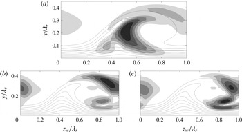
Figure 8.
 $|\tilde{u} _{w}|/\max |\tilde{u} _{w}|$
for the type III mode (a, in figure 7
a) and the ‘harmonics’ of type II (b,c, respectively IIb, IIc in figure 7
b) modes, levels span
$|\tilde{u} _{w}|/\max |\tilde{u} _{w}|$
for the type III mode (a, in figure 7
a) and the ‘harmonics’ of type II (b,c, respectively IIb, IIc in figure 7
b) modes, levels span
 $[1/6,5/6]$
with
$[1/6,5/6]$
with
 $\unicode[STIX]{x1D6E5}=1/6$
. Near-wall region (dash-dotted line).
$\unicode[STIX]{x1D6E5}=1/6$
. Near-wall region (dash-dotted line).
 $\overline{U}_{w}/\overline{U}_{e}$
levels
$\overline{U}_{w}/\overline{U}_{e}$
levels
 $0.1,0.2,\ldots ,0.9$
(dotted).
$0.1,0.2,\ldots ,0.9$
(dotted).
The most typical arrangement of the spectrum is shown in figure 7(b). The unstable modes are, from most to least unstable: the type I mode, the type II (fundamental) mode and the second and third harmonic of the latter, by inspection of the eigenfunctions shown in figures 8(b) and 8(c). These structures correspond closely to those reported by Koch et al. (Reference Koch, Bertolotti, Stolte and Hein2000, cf. figure 16). The Arnoldi algorithm does not return the type III mode for this number of requested solutions in this particular case. For
 $\unicode[STIX]{x1D6FC}\unicode[STIX]{x1D706}_{r}=1$
, the type III mode is contained within the mode horizon, the dashed line in figure 7(a). The location of the type III mode and the line indicating the near-wall limit correspond to the phase speed of the type III mode reported by Bonfigli & Kloker (Reference Bonfigli and Kloker2007). The type III eigenfunction is shown in figure 8(a) and, interestingly, corresponds very closely to the type II/III hybrid shape shown in figure 35 of Bonfigli & Kloker (Reference Bonfigli and Kloker2007). The mode horizon approaches the continuous spectrum very closely in this case, indicating the challenge with tracking the type III mode with the optimized set-up. Analysis of the type III mode falls beyond the scope of the present study and will not be considered in the following discussion.
$\unicode[STIX]{x1D6FC}\unicode[STIX]{x1D706}_{r}=1$
, the type III mode is contained within the mode horizon, the dashed line in figure 7(a). The location of the type III mode and the line indicating the near-wall limit correspond to the phase speed of the type III mode reported by Bonfigli & Kloker (Reference Bonfigli and Kloker2007). The type III eigenfunction is shown in figure 8(a) and, interestingly, corresponds very closely to the type II/III hybrid shape shown in figure 35 of Bonfigli & Kloker (Reference Bonfigli and Kloker2007). The mode horizon approaches the continuous spectrum very closely in this case, indicating the challenge with tracking the type III mode with the optimized set-up. Analysis of the type III mode falls beyond the scope of the present study and will not be considered in the following discussion.
4 Results
4.1 Base spectrum
To give a general overview of the spectrum, the base flow plane conceived with 500 instantaneous snapshots is considered as a reference baseline case. The branches of eigenvalues corresponding to the type I and II modes are shown in figure 9. The temporal global stability problem is solved for the
 $\unicode[STIX]{x1D6FC}$
-range
$\unicode[STIX]{x1D6FC}$
-range
 $[0.5,18]/\unicode[STIX]{x1D706}_{r}$
with a spacing of
$[0.5,18]/\unicode[STIX]{x1D706}_{r}$
with a spacing of
 $0.1/\unicode[STIX]{x1D706}_{r}$
. In the figure, the branches are shown for the
$0.1/\unicode[STIX]{x1D706}_{r}$
. In the figure, the branches are shown for the
 $\unicode[STIX]{x1D6FC}$
-range over which the branches are unstable.
$\unicode[STIX]{x1D6FC}$
-range over which the branches are unstable.
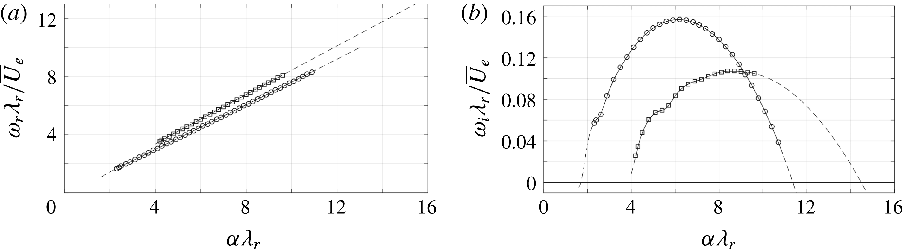
Figure 9. Type I (circles) and II (squares) temporal frequency (a) and growth rate (b) versus the wavenumber using the
 $N_{z}\times N_{y}=55\times 55$
(dashed line) and
$N_{z}\times N_{y}=55\times 55$
(dashed line) and
 $90\times 90$
(solid) grid nodes.
$90\times 90$
(solid) grid nodes.

Figure 10.
 $|\tilde{u} _{w}|/\max |\tilde{u} _{w}|$
for type I (a) and II (b) (levels span
$|\tilde{u} _{w}|/\max |\tilde{u} _{w}|$
for type I (a) and II (b) (levels span
 $[1/6,5/6]$
with
$[1/6,5/6]$
with
 $\unicode[STIX]{x1D6E5}=1/6$
).
$\unicode[STIX]{x1D6E5}=1/6$
).
 $90\times 90$
(filled contours) and
$90\times 90$
(filled contours) and
 $55\times 55$
(dashed) grid resolution. Near-wall region (dash-dotted line).
$55\times 55$
(dashed) grid resolution. Near-wall region (dash-dotted line).
 $\overline{U}_{w}/\overline{U}_{e}$
levels
$\overline{U}_{w}/\overline{U}_{e}$
levels
 $0.1,0.2,\ldots ,0.9$
(dotted).
$0.1,0.2,\ldots ,0.9$
(dotted).
Table 1. Parameters of the (most temporally unstable and POD wavelength) modes in the base spectrum for the strong vortex.
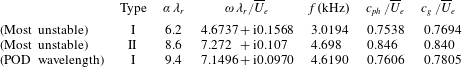
Several grid resolutions are used to compute the spectra with the focused grid for the type I mode, going up to
 $N_{z}\times N_{y}=90\times 90$
nodes. The mode branches are found to be converged already for
$N_{z}\times N_{y}=90\times 90$
nodes. The mode branches are found to be converged already for
 $N_{z}\times N_{y}=55\times 55$
nodes, with eigenvalue errors of
$N_{z}\times N_{y}=55\times 55$
nodes, with eigenvalue errors of
 $O(10^{-5})$
in absolute sense for the type I instability. Despite the lower grid density in the region of dominance of the type II mode, the spectral discretization captures this mode properly as well. The most unstable type II eigenvalue experiences a
$O(10^{-5})$
in absolute sense for the type I instability. Despite the lower grid density in the region of dominance of the type II mode, the spectral discretization captures this mode properly as well. The most unstable type II eigenvalue experiences a
 $O(10^{-4})$
absolute error, which is deemed sufficiently small for the purposes of this analysis.
$O(10^{-4})$
absolute error, which is deemed sufficiently small for the purposes of this analysis.
The type I mode attains the maximum temporal growth rate and is therefore locally most unstable. The type II mode is found to be locally more unstable for
 $\unicode[STIX]{x1D714}_{r}>7.77\overline{U}_{e}/\unicode[STIX]{x1D706}_{r}=5.0~\text{kHz}$
. The spectral information associated with the locally most unstable type I and II modes is given in table 1. It is important to note that these indications do not directly imply these modes are the largest perturbation at this station. To investigate that, the local results, in terms of the spatial amplification rate, have to be integrated in space, i.e.
$\unicode[STIX]{x1D714}_{r}>7.77\overline{U}_{e}/\unicode[STIX]{x1D706}_{r}=5.0~\text{kHz}$
. The spectral information associated with the locally most unstable type I and II modes is given in table 1. It is important to note that these indications do not directly imply these modes are the largest perturbation at this station. To investigate that, the local results, in terms of the spatial amplification rate, have to be integrated in space, i.e.
 $N$
-factors should be considered.
$N$
-factors should be considered.
The
 $|\tilde{u} |$
-eigenfunctions corresponding to the most unstable type I and II modes are shown in figure 10. The spatial distributions of the modes are superimposed over the isocontours of the streamwise velocity of the base flow. Previous investigations from both numerical and experimental perspectives, see Malik et al. (Reference Malik, Li and Chang1994), White & Saric (Reference White and Saric2005), Bonfigli & Kloker (Reference Bonfigli and Kloker2007), indicate the type I mode is positioned on the outer upwashing side of the primary vortex, close to the in-plane saddle point, while the type II mode rides on top of the vortex. As evident, these characteristics are well captured by the stability analysis. Two spatial mode distributions are to be distinguished in figures 10(a) and 10(b) and correspond to different grid resolutions. The difference is small, further confirming that the
$|\tilde{u} |$
-eigenfunctions corresponding to the most unstable type I and II modes are shown in figure 10. The spatial distributions of the modes are superimposed over the isocontours of the streamwise velocity of the base flow. Previous investigations from both numerical and experimental perspectives, see Malik et al. (Reference Malik, Li and Chang1994), White & Saric (Reference White and Saric2005), Bonfigli & Kloker (Reference Bonfigli and Kloker2007), indicate the type I mode is positioned on the outer upwashing side of the primary vortex, close to the in-plane saddle point, while the type II mode rides on top of the vortex. As evident, these characteristics are well captured by the stability analysis. Two spatial mode distributions are to be distinguished in figures 10(a) and 10(b) and correspond to different grid resolutions. The difference is small, further confirming that the
 $55\times 55$
grid yields converged eigensolutions.
$55\times 55$
grid yields converged eigensolutions.
Using the Reynolds–Orr equation (3.3), the most unstable type I and II eigenmodes can be decomposed into the most dominant contributions shown in figure 11, ordered from absolute largest to smallest top to bottom. The remainder is composed out of terms that are individually smaller than the dominant terms in absolute value. The eigenvalues themselves are indicated with dashed lines. Two bars are given for each term, again corresponding to different grid resolutions. The differences in the contributions are consistent with the errors in the eigenvalues.
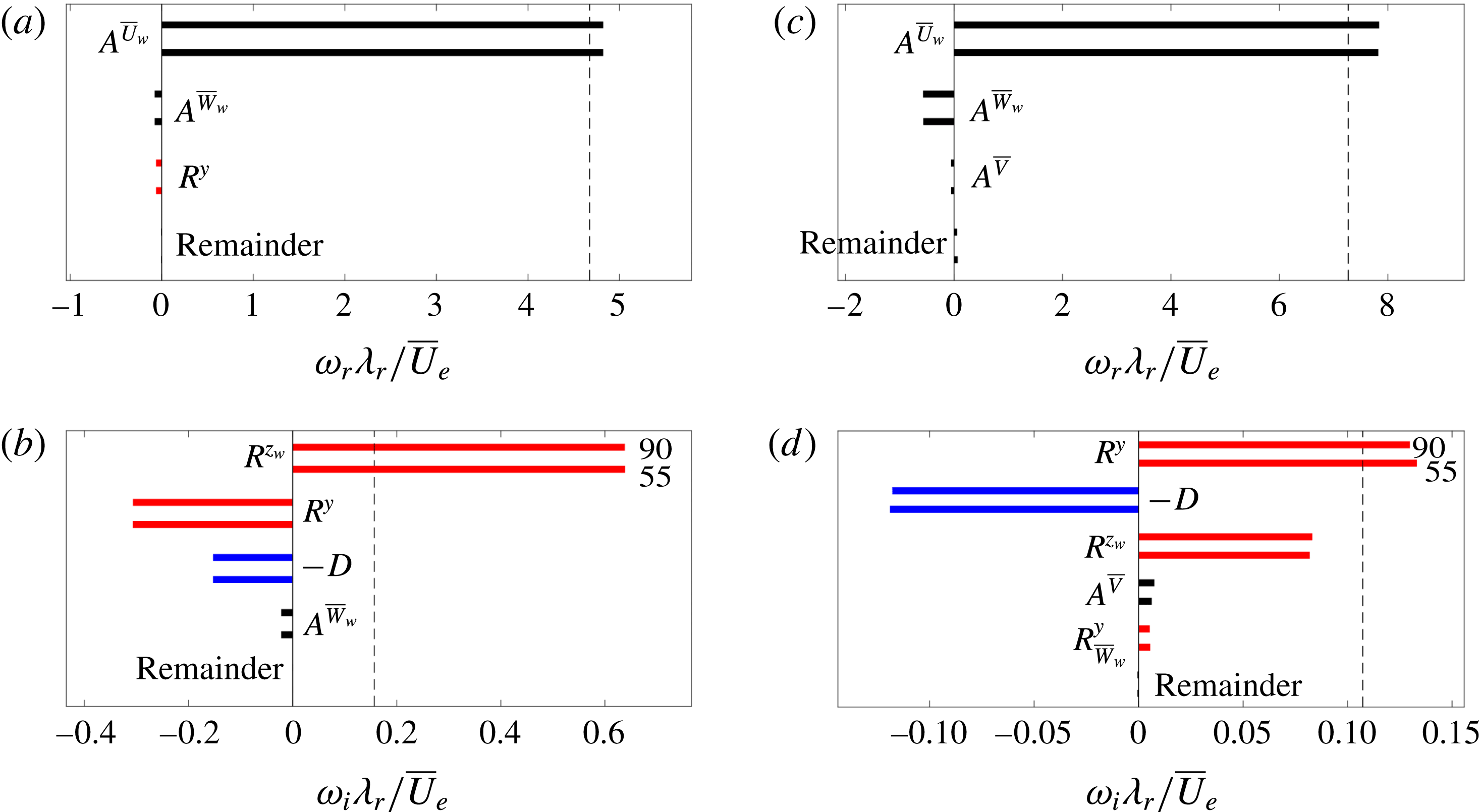
Figure 11. (a,c)
 $\unicode[STIX]{x1D714}_{r}$
- and (b,d)
$\unicode[STIX]{x1D714}_{r}$
- and (b,d)
 $\unicode[STIX]{x1D714}_{i}$
-budgets (bars) of type I (a,b) and II (c,d),
$\unicode[STIX]{x1D714}_{i}$
-budgets (bars) of type I (a,b) and II (c,d),
 $\unicode[STIX]{x1D714}$
eigenvalue (dashed line). Reynolds stress, viscous dissipation and advection terms are coloured red, blue and black, respectively, see equation (3.6) for symbol definitions. Upper bars:
$\unicode[STIX]{x1D714}$
eigenvalue (dashed line). Reynolds stress, viscous dissipation and advection terms are coloured red, blue and black, respectively, see equation (3.6) for symbol definitions. Upper bars:
 $90\times 90$
, lower bars:
$90\times 90$
, lower bars:
 $55\times 55$
grid resolution.
$55\times 55$
grid resolution.
The
 $\unicode[STIX]{x1D714}_{i}$
-budget for both mode types is most dominantly dictated by the
$\unicode[STIX]{x1D714}_{i}$
-budget for both mode types is most dominantly dictated by the
 $\overline{U}_{w}$
-shear and viscous dissipation. As per the definitions proposed by Malik et al. (Reference Malik, Li and Chang1996), the type I and II (or,
$\overline{U}_{w}$
-shear and viscous dissipation. As per the definitions proposed by Malik et al. (Reference Malik, Li and Chang1996), the type I and II (or,
 $z$
- and
$z$
- and
 $y$
-) modes are produced by the
$y$
-) modes are produced by the
 $\unicode[STIX]{x2202}\overline{U}_{w}/\unicode[STIX]{x2202}z_{w}$
and
$\unicode[STIX]{x2202}\overline{U}_{w}/\unicode[STIX]{x2202}z_{w}$
and
 $\unicode[STIX]{x2202}\overline{U}_{w}/\unicode[STIX]{x2202}y$
shear components, respectively. This is found in the current case as well, as shown in figure 11(b,d). The other shear components are usually unimportant and can have a net destructive nature, as is the case for the type I mode here. Figure 11(d) illustrates this is not the case for the type II mode; in that case the
$\unicode[STIX]{x2202}\overline{U}_{w}/\unicode[STIX]{x2202}y$
shear components, respectively. This is found in the current case as well, as shown in figure 11(b,d). The other shear components are usually unimportant and can have a net destructive nature, as is the case for the type I mode here. Figure 11(d) illustrates this is not the case for the type II mode; in that case the
 $\unicode[STIX]{x2202}\overline{U}_{w}/\unicode[STIX]{x2202}z_{w}$
shear also has a significant net productive role. Modes for which both production terms have comparable contributions are referred to as
$\unicode[STIX]{x2202}\overline{U}_{w}/\unicode[STIX]{x2202}z_{w}$
shear also has a significant net productive role. Modes for which both production terms have comparable contributions are referred to as
 $y/z$
-modes, see Li et al. (Reference Li, Choudhari, Duan and Chang2014).
$y/z$
-modes, see Li et al. (Reference Li, Choudhari, Duan and Chang2014).
Having pinpointed the Reynolds stress terms as most prominent in the
 $\unicode[STIX]{x1D714}_{i}$
-budget, further insight into their spatial topology is sought. Figure 12 shows the integrands of
$\unicode[STIX]{x1D714}_{i}$
-budget, further insight into their spatial topology is sought. Figure 12 shows the integrands of
 $R^{y}$
and
$R^{y}$
and
 $R^{z_{w}}$
for both modes in the plane. After integration over the plane, these functions yield the contributions shown in figure 11(b,d). These terms have their origin in the
$R^{z_{w}}$
for both modes in the plane. After integration over the plane, these functions yield the contributions shown in figure 11(b,d). These terms have their origin in the
 $x_{w}$
-momentum equation (3.2a
) and hence directly produce the
$x_{w}$
-momentum equation (3.2a
) and hence directly produce the
 $\tilde{u} _{w}$
(energy) component. The integrands therefore indicate which part of the
$\tilde{u} _{w}$
(energy) component. The integrands therefore indicate which part of the
 $\tilde{u} _{w}$
eigenfunction they produce. For the type I mode, the integrands clearly reflect the integral values. Interestingly, the downward protrusion located about
$\tilde{u} _{w}$
eigenfunction they produce. For the type I mode, the integrands clearly reflect the integral values. Interestingly, the downward protrusion located about
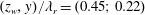 $(z_{w},y)/\unicode[STIX]{x1D706}_{r}=(0.45;0.22)$
is produced by the
$(z_{w},y)/\unicode[STIX]{x1D706}_{r}=(0.45;0.22)$
is produced by the
 $R^{y}$
-term; as illustrated with the additional contours in figure 12(a). The integrands for the type II mode are surprising, because the integrand of
$R^{y}$
-term; as illustrated with the additional contours in figure 12(a). The integrands for the type II mode are surprising, because the integrand of
 $R^{z_{w}}$
attains the largest value, while the
$R^{z_{w}}$
attains the largest value, while the
 $z_{w}y$
-integral value is smaller. The shape of the positive
$z_{w}y$
-integral value is smaller. The shape of the positive
 $R^{y}$
- and
$R^{y}$
- and
 $R^{z_{w}}$
-integrand contours is comparable to that by Malik et al. (Reference Malik, Li, Choudhari and Chang1999) (cf. figure 10).
$R^{z_{w}}$
-integrand contours is comparable to that by Malik et al. (Reference Malik, Li, Choudhari and Chang1999) (cf. figure 10).
As mentioned, the participation of the advection terms
 $A^{\overline{V}}$
and
$A^{\overline{V}}$
and
 $A^{\overline{W}_{w}}$
is not restricted to the real dispersion dynamics; as pointed out in figure 11(b,d), they are the next terms in line enhancing or reducing the growth rates of the modes, confirming the inclusion of the
$A^{\overline{W}_{w}}$
is not restricted to the real dispersion dynamics; as pointed out in figure 11(b,d), they are the next terms in line enhancing or reducing the growth rates of the modes, confirming the inclusion of the
 $\overline{V}$
- and
$\overline{V}$
- and
 $\overline{W}_{w}$
-components in the analysis is essential. With respect to
$\overline{W}_{w}$
-components in the analysis is essential. With respect to
 $\unicode[STIX]{x1D714}_{i}$
,
$\unicode[STIX]{x1D714}_{i}$
,
 $A^{\overline{V}}$
and
$A^{\overline{V}}$
and
 $A^{\overline{W}_{w}}$
respectively exert 2.4% and
$A^{\overline{W}_{w}}$
respectively exert 2.4% and
 $-14.1\%$
contributions for the type I and 7.0% and 2.8% contributions for the type II mode. Figure 11(b,d) shows some of these values are larger than the Reynolds stress terms associated with these velocity components.
$-14.1\%$
contributions for the type I and 7.0% and 2.8% contributions for the type II mode. Figure 11(b,d) shows some of these values are larger than the Reynolds stress terms associated with these velocity components.
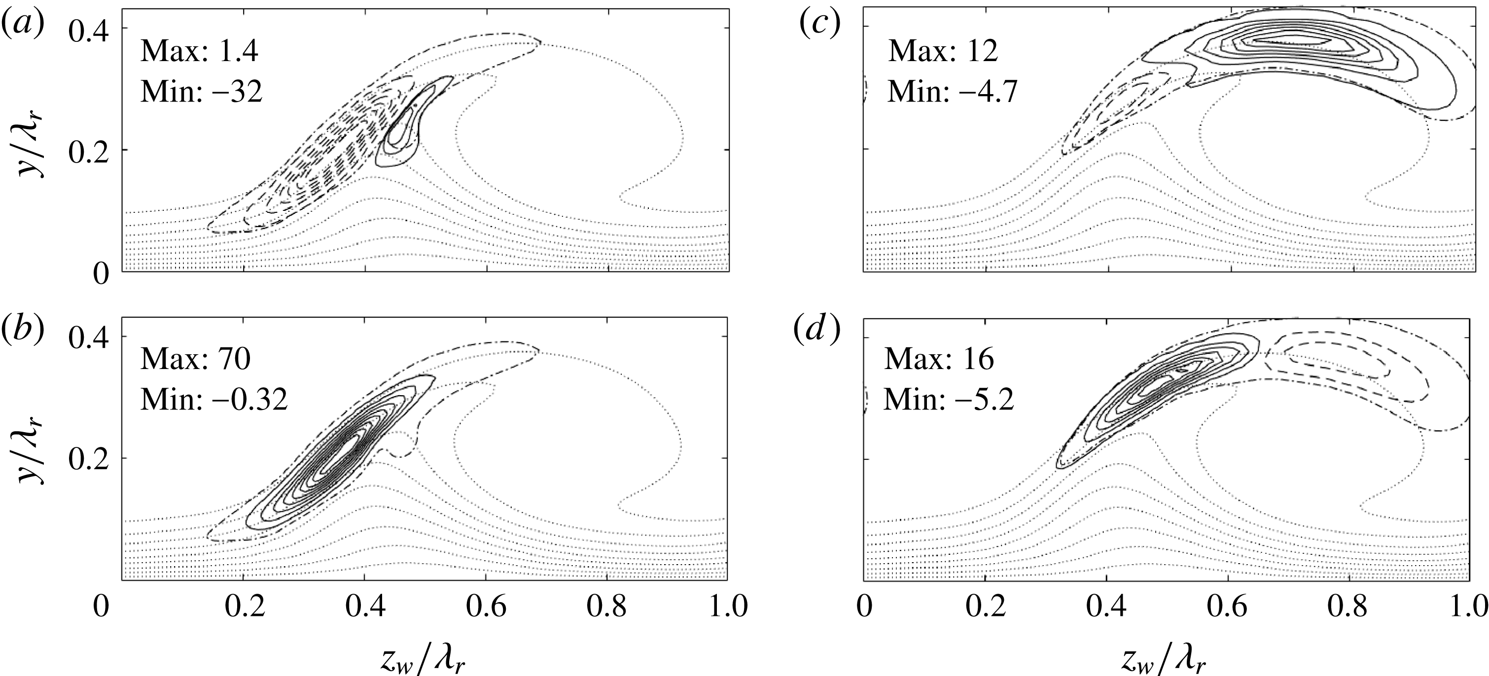
Figure 12. Imaginary part of the (a,c)
 $R^{y}$
- and (b,d)
$R^{y}$
- and (b,d)
 $R^{z_{w}}$
-integrands for type I (a,b) and II (c,d) (9 levels span (b)
$R^{z_{w}}$
-integrands for type I (a,b) and II (c,d) (9 levels span (b)
 $[6.71,63.0]$
, (c)
$[6.71,63.0]$
, (c)
 $[-3.00,10.4]$
and (d)
$[-3.00,10.4]$
and (d)
 $[-3.07,14.1]$
, negative contours are dashed). Levels in (a) span
$[-3.07,14.1]$
, negative contours are dashed). Levels in (a) span
 $[-27.5,-3.41]$
, with
$[-27.5,-3.41]$
, with
 $\unicode[STIX]{x1D6E5}=4.83$
, and
$\unicode[STIX]{x1D6E5}=4.83$
, and
 $[0.350,1.05]$
,
$[0.350,1.05]$
,
 $\unicode[STIX]{x1D6E5}=0.350$
. All values are given in
$\unicode[STIX]{x1D6E5}=0.350$
. All values are given in
 $\overline{U}_{e}/\unicode[STIX]{x1D706}_{r}^{3}$
-units. Eigenfunction contour
$\overline{U}_{e}/\unicode[STIX]{x1D706}_{r}^{3}$
-units. Eigenfunction contour
 $|\tilde{u} _{w}|/\max |\tilde{u} _{w}|=1/6$
(dash-dotted line).
$|\tilde{u} _{w}|/\max |\tilde{u} _{w}|=1/6$
(dash-dotted line).
 $\overline{U}_{w}/\overline{U}_{e}$
levels
$\overline{U}_{w}/\overline{U}_{e}$
levels
 $0.1,0.2,\ldots ,0.9$
(dotted).
$0.1,0.2,\ldots ,0.9$
(dotted).
The origin of the growth induced by the in-plane advection is traced by visualizing the integrands of the related terms in the Reynolds–Orr equation. The previous numbers illustrate
 $A^{\overline{V}}$
and
$A^{\overline{V}}$
and
 $A^{\overline{W}_{w}}$
individually yield a predominant decrease and increase in the type II and type I growth rates, respectively. Figure 13(a,b,d,e) shows the integrands associated with
$A^{\overline{W}_{w}}$
individually yield a predominant decrease and increase in the type II and type I growth rates, respectively. Figure 13(a,b,d,e) shows the integrands associated with
 $A^{\overline{V}}$
and
$A^{\overline{V}}$
and
 $A^{\overline{W}_{w}}$
for both modes. The sign of the sum of these terms is illustrated in figure 13(c,f), indicating the (de)stabilizing regions. The latter panels clearly reflect the criterion based on the term (3.7); whenever the in-plane flow is directed away from elevated perturbation levels, the contribution is destabilizing (black arrows). Conversely, whenever the in-plane velocity is aligned with the perturbation level gradient, the contribution is stabilizing. Contours of the sum of the amplitudes
$A^{\overline{W}_{w}}$
for both modes. The sign of the sum of these terms is illustrated in figure 13(c,f), indicating the (de)stabilizing regions. The latter panels clearly reflect the criterion based on the term (3.7); whenever the in-plane flow is directed away from elevated perturbation levels, the contribution is destabilizing (black arrows). Conversely, whenever the in-plane velocity is aligned with the perturbation level gradient, the contribution is stabilizing. Contours of the sum of the amplitudes
 $|\tilde{u} _{w}|+|\tilde{v}|+|\tilde{w}_{w}|$
are shown, because (3.7) features the gradient of the velocity amplitudes, not the (square root of the) perturbation energy. In the case of the type I mode, the in-plane flow has the tendency to focus the perturbation energy along a spanwise line and therefore has the major effect of increasing the spanwise extent of the eigenfunction. On the other hand, the eigenfunction’s maximum is located close to the in-plane flow saddle. This location is thus affected to a minor extent only. For the type II mode, the main effect is advection in the
$|\tilde{u} _{w}|+|\tilde{v}|+|\tilde{w}_{w}|$
are shown, because (3.7) features the gradient of the velocity amplitudes, not the (square root of the) perturbation energy. In the case of the type I mode, the in-plane flow has the tendency to focus the perturbation energy along a spanwise line and therefore has the major effect of increasing the spanwise extent of the eigenfunction. On the other hand, the eigenfunction’s maximum is located close to the in-plane flow saddle. This location is thus affected to a minor extent only. For the type II mode, the main effect is advection in the
 $z_{w}$
-direction. Therefore it is expected that the location of the eigenfunction’s maximum is sensitive to small changes in the productive Reynolds stress. Note that the integrand magnitudes of the advection terms for the type II mode are comparable with those of the Reynolds stresses, while they are an order of magnitude smaller for the type I mode.
$z_{w}$
-direction. Therefore it is expected that the location of the eigenfunction’s maximum is sensitive to small changes in the productive Reynolds stress. Note that the integrand magnitudes of the advection terms for the type II mode are comparable with those of the Reynolds stresses, while they are an order of magnitude smaller for the type I mode.
Figure 13. (a,b,d,e) Imaginary part of (a,d)
 $A^{\overline{V}}$
- and (b,e)
$A^{\overline{V}}$
- and (b,e)
 $A^{\overline{W}_{w}}$
-integrands for type I (a,b) and II (d,e) (9 levels ranging (a)
$A^{\overline{W}_{w}}$
-integrands for type I (a,b) and II (d,e) (9 levels ranging (a)
 $[-6.84,5.78]$
, (b)
$[-6.84,5.78]$
, (b)
 $[-8.74,6.68]$
, (d)
$[-8.74,6.68]$
, (d)
 $[-6.43,5.93]$
and (e)
$[-6.43,5.93]$
and (e)
 $[-8.99,4.32]$
in
$[-8.99,4.32]$
in
 $\overline{U}_{e}/\unicode[STIX]{x1D706}_{r}^{3}$
-units, negative contours are dashed). Eigenfunction contour
$\overline{U}_{e}/\unicode[STIX]{x1D706}_{r}^{3}$
-units, negative contours are dashed). Eigenfunction contour
 $|\tilde{u} _{w}|/\max |\tilde{u} _{w}|=1/6$
(dash-dotted line). (c,f) (
$|\tilde{u} _{w}|/\max |\tilde{u} _{w}|=1/6$
(dash-dotted line). (c,f) (
 $\overline{V},\overline{W}_{w}$
)-vectors showing where
$\overline{V},\overline{W}_{w}$
)-vectors showing where
 $\text{Im}\{A^{\overline{V}}+A^{\overline{W}_{w}}\}<0$
(white arrows) and
$\text{Im}\{A^{\overline{V}}+A^{\overline{W}_{w}}\}<0$
(white arrows) and
 ${>}0$
(black arrows) for type I (c) and II (f). Amplitude sum
${>}0$
(black arrows) for type I (c) and II (f). Amplitude sum
 $|\tilde{u} _{w}|+|\tilde{v}|+|\tilde{w}_{w}|$
(6 filled contours from 0 to maximum).
$|\tilde{u} _{w}|+|\tilde{v}|+|\tilde{w}_{w}|$
(6 filled contours from 0 to maximum).
 $\overline{U}_{w}/\overline{U}_{e}$
levels
$\overline{U}_{w}/\overline{U}_{e}$
levels
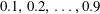 $0.1,0.2,\ldots ,0.9$
(dotted).
$0.1,0.2,\ldots ,0.9$
(dotted).
A large stabilizing pocket is visible in figure 13(b), for which
 $\overline{W}_{w}>0$
and
$\overline{W}_{w}>0$
and
 $\tilde{\boldsymbol{q}}^{\ast }\boldsymbol{\cdot }\unicode[STIX]{x2202}\tilde{\boldsymbol{q}}/\unicode[STIX]{x2202}z_{w}>0$
, above the in-plane flow saddle. That region largely contributes to the net
$\tilde{\boldsymbol{q}}^{\ast }\boldsymbol{\cdot }\unicode[STIX]{x2202}\tilde{\boldsymbol{q}}/\unicode[STIX]{x2202}z_{w}>0$
, above the in-plane flow saddle. That region largely contributes to the net
 $\overline{W}_{w}$
-advection towards the shear layer’s core causing the negative integral value for the type I mode. The magnitude of
$\overline{W}_{w}$
-advection towards the shear layer’s core causing the negative integral value for the type I mode. The magnitude of
 $A^{\overline{V}}$
in the energy budget for the type II mode is approximately 3 times smaller than
$A^{\overline{V}}$
in the energy budget for the type II mode is approximately 3 times smaller than
 $A^{\overline{W}_{w}}$
for type I. This is reflected by more evenly matched levels in figure 13(d). The positive contribution in figure 11(d) indicates a net
$A^{\overline{W}_{w}}$
for type I. This is reflected by more evenly matched levels in figure 13(d). The positive contribution in figure 11(d) indicates a net
 $\overline{V}$
-advection away from the core of the shear layer. The largest contours in figure 13(d) indicate this is largely associated with an imbalance of vertical in- and outward advection on the left-hand side of the vortex core. The contours in figure 13(a,e) display a symmetric shape with respect to the absolute eigenfunction contour itself relative to the other cases, explaining negligible integral values. All contours in figure 13 are contained within the region of dominance of the Reynolds stress terms and hence do not generate additional eigenfunction features. Nonetheless, it is noteworthy that the contours in figure 13(a,b,d,e) reach the outer limits of the eigenfunction, especially the top right of the type I mode at which the Reynolds stress terms are an order of magnitude smaller.
$\overline{V}$
-advection away from the core of the shear layer. The largest contours in figure 13(d) indicate this is largely associated with an imbalance of vertical in- and outward advection on the left-hand side of the vortex core. The contours in figure 13(a,e) display a symmetric shape with respect to the absolute eigenfunction contour itself relative to the other cases, explaining negligible integral values. All contours in figure 13 are contained within the region of dominance of the Reynolds stress terms and hence do not generate additional eigenfunction features. Nonetheless, it is noteworthy that the contours in figure 13(a,b,d,e) reach the outer limits of the eigenfunction, especially the top right of the type I mode at which the Reynolds stress terms are an order of magnitude smaller.
For both modes,
 $A^{\overline{U}_{w}}$
yields the largest contribution to
$A^{\overline{U}_{w}}$
yields the largest contribution to
 $\unicode[STIX]{x1D714}_{r}$
. The action of the in-plane velocity components is to retard the secondary vortices’ advection in the
$\unicode[STIX]{x1D714}_{r}$
. The action of the in-plane velocity components is to retard the secondary vortices’ advection in the
 $x_{w}$
-direction. In total,
$x_{w}$
-direction. In total,
 $A^{\overline{U}_{w}}$
is cancelled to 3.1 % and 7.1 % by other terms for the type I and II modes, respectively. The large retardation in the case of the type II mode, considering that the other terms cancel out, is solely caused by
$A^{\overline{U}_{w}}$
is cancelled to 3.1 % and 7.1 % by other terms for the type I and II modes, respectively. The large retardation in the case of the type II mode, considering that the other terms cancel out, is solely caused by
 $\overline{W}_{w}$
. This is interpreted to be the consequence of the fact that the eigenmodes travel in the opposite direction of
$\overline{W}_{w}$
. This is interpreted to be the consequence of the fact that the eigenmodes travel in the opposite direction of
 $\overline{W}_{w}$
. No singular such term can be pointed out for the type I mode. An example of a Reynolds stress term participating in the
$\overline{W}_{w}$
. No singular such term can be pointed out for the type I mode. An example of a Reynolds stress term participating in the
 $\unicode[STIX]{x1D714}_{r}$
-budget is
$\unicode[STIX]{x1D714}_{r}$
-budget is
 $R^{y}$
, that slightly reduces the type I mode frequency.
$R^{y}$
, that slightly reduces the type I mode frequency.
4.2 Effect of ensemble size
The measured mean flow is subject to an uncertainty of
 $0.1\overline{U}_{e}/\sqrt{500}=4.5\times 10^{-3}\overline{U}_{e}$
, based on the maximum r.m.s. amplitude of
$0.1\overline{U}_{e}/\sqrt{500}=4.5\times 10^{-3}\overline{U}_{e}$
, based on the maximum r.m.s. amplitude of
 $0.1\overline{U}_{e}$
obtained from the 500 instantaneous PIV snapshots (see § 4.6). The reported uncertainty stems from both systematic errors (such as tomo-PIV correlation errors), as well as from physical fluctuations of the instantaneous flow. For instance, Serpieri & Kotsonis (Reference Serpieri and Kotsonis2016) (cf. § 6.3.1) show the r.m.s. field is dominated by a low-frequency spanwise shake of the whole primary crossflow vortex, obtained as the most energetic POD mode. While these are acceptable uncertainty levels for flow diagnostics, their effect on the stability analysis should be carefully identified. In this section an effort is provided towards quantifying the effect of the ensemble average on the eigensolutions.
$0.1\overline{U}_{e}$
obtained from the 500 instantaneous PIV snapshots (see § 4.6). The reported uncertainty stems from both systematic errors (such as tomo-PIV correlation errors), as well as from physical fluctuations of the instantaneous flow. For instance, Serpieri & Kotsonis (Reference Serpieri and Kotsonis2016) (cf. § 6.3.1) show the r.m.s. field is dominated by a low-frequency spanwise shake of the whole primary crossflow vortex, obtained as the most energetic POD mode. While these are acceptable uncertainty levels for flow diagnostics, their effect on the stability analysis should be carefully identified. In this section an effort is provided towards quantifying the effect of the ensemble average on the eigensolutions.
The uncertainty is quantified by deploying a Monte Carlo approach to the stability analysis. More specifically, stability analysis is performed on mean flows produced by varying the ensemble size,
 $N_{fr}$
, ranging from 300 to 475, with steps of 25. One hundred different random combinations are made per
$N_{fr}$
, ranging from 300 to 475, with steps of 25. One hundred different random combinations are made per
 $N_{fr}$
from the total pool of 500 snapshots, resulting in 800 cases in total plus the single case possible for
$N_{fr}$
from the total pool of 500 snapshots, resulting in 800 cases in total plus the single case possible for
 $N_{fr}=500$
; used as the baseline case. Stability simulations were performed on the
$N_{fr}=500$
; used as the baseline case. Stability simulations were performed on the
 $45.6\,\%$
chord plane using the
$45.6\,\%$
chord plane using the
 $55\times 55$
grid. For both modes, the respective most unstable wavenumber in table 1 was used as input.
$55\times 55$
grid. For both modes, the respective most unstable wavenumber in table 1 was used as input.
The results are shown in terms of the mean and 2 standard deviations (
 $\pm 2\unicode[STIX]{x1D70E}$
) of the growth rate in relation to the ensemble size in figure 14. While the solution undergoes large fluctuations for small ensemble sizes, which is expected, a clear convergence trend is established for both the mean value and fluctuations. The difference between the estimated mean growth rate for
$\pm 2\unicode[STIX]{x1D70E}$
) of the growth rate in relation to the ensemble size in figure 14. While the solution undergoes large fluctuations for small ensemble sizes, which is expected, a clear convergence trend is established for both the mean value and fluctuations. The difference between the estimated mean growth rate for
 $N_{fr}=450$
and the single case growth rate for
$N_{fr}=450$
and the single case growth rate for
 $N_{fr}=500$
is given in table 2 as
$N_{fr}=500$
is given in table 2 as
 $\unicode[STIX]{x0394}\unicode[STIX]{x1D707}$
, illustrating convergence of the mean to errors at most one order of magnitude larger than the grid truncation errors. The percentages in the table are the relative errors with respect to the value for the
$\unicode[STIX]{x0394}\unicode[STIX]{x1D707}$
, illustrating convergence of the mean to errors at most one order of magnitude larger than the grid truncation errors. The percentages in the table are the relative errors with respect to the value for the
 $N_{fr}=500$
case.
$N_{fr}=500$
case.
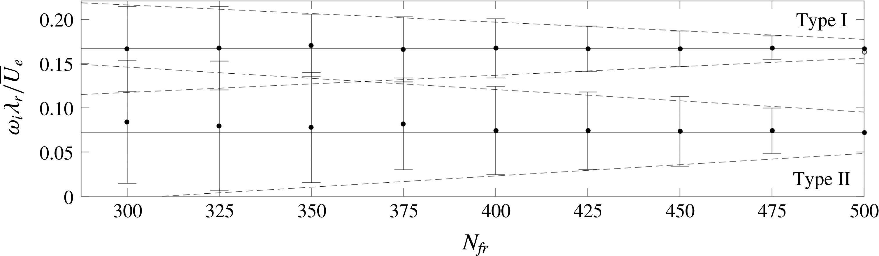
Figure 14. Growth rate uncertainty versus ensemble size
 $N_{fr}$
for both instability modes. Mean (dots) and 2
$N_{fr}$
for both instability modes. Mean (dots) and 2
 $\unicode[STIX]{x1D70E}$
(bars) based on 100 random combinations for fixed
$\unicode[STIX]{x1D70E}$
(bars) based on 100 random combinations for fixed
 $N_{fr}$
. The dots at
$N_{fr}$
. The dots at
 $N_{fr}=500$
and horizontal lines are the calculated eigenvalue itself. Linear fit to the 2
$N_{fr}=500$
and horizontal lines are the calculated eigenvalue itself. Linear fit to the 2
 $\unicode[STIX]{x1D70E}$
-bars (dashed lines).
$\unicode[STIX]{x1D70E}$
-bars (dashed lines).
Table 2. Uncertainty and errors in type I and II mode parameters with ensemble size (§ 4.2) and domain extrapolation parameters (handled in § 4.4).
 $^{\dagger }z_{w}$
is based on
$^{\dagger }z_{w}$
is based on
 $N_{fr}=475$
, avoiding extrapolation.
$N_{fr}=475$
, avoiding extrapolation.
The growth rate fluctuations within the 100 random cases are relatively large as shown by the standard deviation bars. Nevertheless, they also show an evident linear converging trend, illustrating that the mean value is approached in the limit of large
 $N_{fr}$
. The linear trend is extrapolated to obtain a measure at
$N_{fr}$
. The linear trend is extrapolated to obtain a measure at
 $N_{fr}=500$
, also reported in table 2. The demonstrated trend allows discarding the fluctuations, under the condition that a minimum threshold
$N_{fr}=500$
, also reported in table 2. The demonstrated trend allows discarding the fluctuations, under the condition that a minimum threshold
 $N_{fr}$
can be defined beyond which the integrity of the solution structure can be demonstrated.
$N_{fr}$
can be defined beyond which the integrity of the solution structure can be demonstrated.
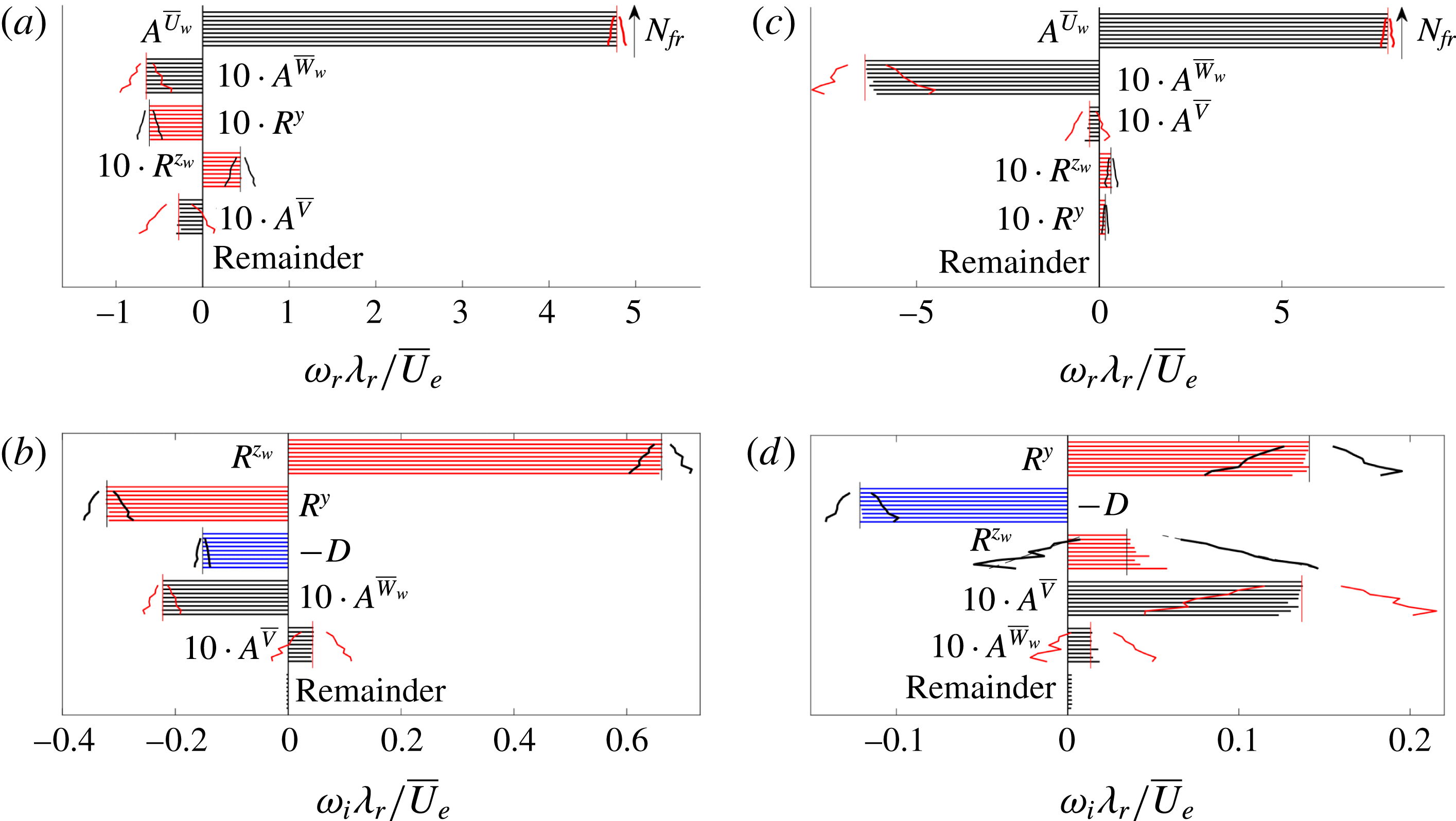
Figure 15. (a,c)
 $\unicode[STIX]{x1D714}_{r}$
- and (b,d)
$\unicode[STIX]{x1D714}_{r}$
- and (b,d)
 $\unicode[STIX]{x1D714}_{i}$
-budgets of type I (a,b) and II (c,d), mean value (bars) and
$\unicode[STIX]{x1D714}_{i}$
-budgets of type I (a,b) and II (c,d), mean value (bars) and
 $2\unicode[STIX]{x1D70E}$
(slanted lines) per
$2\unicode[STIX]{x1D70E}$
(slanted lines) per
 $N_{fr}$
, ranging from 300 (bottom bar) to 500 (top bar) every 25 samples. Vertical lines indicate the single eigensolution for
$N_{fr}$
, ranging from 300 (bottom bar) to 500 (top bar) every 25 samples. Vertical lines indicate the single eigensolution for
 $N_{fr}=500$
as a reference. Small terms (mean and
$N_{fr}=500$
as a reference. Small terms (mean and
 $2\unicode[STIX]{x1D70E}$
) are magnified with a factor 10, the slanted lines then indicate
$2\unicode[STIX]{x1D70E}$
) are magnified with a factor 10, the slanted lines then indicate
 $20\unicode[STIX]{x1D70E}$
.
$20\unicode[STIX]{x1D70E}$
.
The terms in the Reynolds–Orr equation are shown as a function of the ensemble size in figure 15. Fluctuations appear, as expected, but the mean term values per
 $N_{fr}$
are well defined and indicate a consistent balance for all
$N_{fr}$
are well defined and indicate a consistent balance for all
 $N_{fr}$
. Note that some contribution values, including the standard deviations with respect to the mean value, are enlarged by a factor 10 for clarity. For the type II mode the mean value of the Reynolds stress terms
$N_{fr}$
. Note that some contribution values, including the standard deviations with respect to the mean value, are enlarged by a factor 10 for clarity. For the type II mode the mean value of the Reynolds stress terms
 $R^{y}$
and
$R^{y}$
and
 $R^{z_{w}}$
changes considerably, albeit only for
$R^{z_{w}}$
changes considerably, albeit only for
 $N_{fr}\leqslant 375$
and the same relative size is retained with respect to the other terms.
$N_{fr}\leqslant 375$
and the same relative size is retained with respect to the other terms.
Prior to physical underpinning of the energy term fluctuations, it is necessary to confirm whether these are influenced by the numerical treatment and discretization of the problem. To this goal, preliminary simulations were performed by altering several parameters. These included increasing the grid resolution from
 $N_{z}\times N_{y}=55\times 55$
to
$N_{z}\times N_{y}=55\times 55$
to
 $90\times 90$
and changing the mean flow differentiation method from a sixth- to fourth-order finite difference scheme. Both changes yielded negligible differences in the stability results, corroborating to a physical mechanism as source of the energy term fluctuations.
$90\times 90$
and changing the mean flow differentiation method from a sixth- to fourth-order finite difference scheme. Both changes yielded negligible differences in the stability results, corroborating to a physical mechanism as source of the energy term fluctuations.
Based on the previous, the fluctuations are concluded to be caused by the physical response of the instability modes to base flow changes. Figure 15(b,d) indicates that growth rate fluctuations are mainly induced by the fluctuations in the Reynolds stresses
 $R^{y}$
and
$R^{y}$
and
 $R^{z_{w}}$
and viscous dissipation
$R^{z_{w}}$
and viscous dissipation
 $D$
. Correlation analysis is used to quantify the link, using all 800 simulation results (all random combinations for all
$D$
. Correlation analysis is used to quantify the link, using all 800 simulation results (all random combinations for all
 $N_{fr}$
). The correlation coefficient between the combination of the Reynolds stress and dissipation terms (
$N_{fr}$
). The correlation coefficient between the combination of the Reynolds stress and dissipation terms (
 $R^{y}+R^{z_{w}}-D$
) on one hand and the growth rate
$R^{y}+R^{z_{w}}-D$
) on one hand and the growth rate
 $\unicode[STIX]{x1D714}_{i}$
on the other are found to be 0.988 and 0.995 for the type I and II modes, respectively. The dissipation evidently adapts itself to the Reynolds stress terms, which is supported by correlation coefficients larger than 0.958 when omitting the dissipation terms (correlating
$\unicode[STIX]{x1D714}_{i}$
on the other are found to be 0.988 and 0.995 for the type I and II modes, respectively. The dissipation evidently adapts itself to the Reynolds stress terms, which is supported by correlation coefficients larger than 0.958 when omitting the dissipation terms (correlating
 $R^{y}+R^{z_{w}}$
to
$R^{y}+R^{z_{w}}$
to
 $\unicode[STIX]{x1D714}_{i}$
).
$\unicode[STIX]{x1D714}_{i}$
).
For the type I mode, the fluctuations in the Reynolds–Orr terms are relatively small and never change the energy balance structurally. Additionally, the advection terms for this mode, although small in the mean, display weak fluctuations. The fluctuations are small enough that the relative size of the terms in the energy balance is fixed qualitatively; they do not break its structure. This is not the case for the type II mode. Especially the
 $R^{z_{w}}$
-term experiences fluctuations large enough to drive the term to negative values (
$R^{z_{w}}$
-term experiences fluctuations large enough to drive the term to negative values (
 $R^{z_{w}}<0$
) on the one hand and larger values than the dominating Reynolds stress term (
$R^{z_{w}}<0$
) on the one hand and larger values than the dominating Reynolds stress term (
 $R^{z_{w}}>R^{y}$
) on the other for different random ensembles for fixed
$R^{z_{w}}>R^{y}$
) on the other for different random ensembles for fixed
 $N_{fr}$
. Nevertheless, all fluctuations show a linear convergence trend with
$N_{fr}$
. Nevertheless, all fluctuations show a linear convergence trend with
 $N_{fr}$
, similar to the eigenvalue in figure 14.
$N_{fr}$
, similar to the eigenvalue in figure 14.
 $A^{\overline{V}}$
displays relatively small fluctuations for type II.
$A^{\overline{V}}$
displays relatively small fluctuations for type II.
The shear values at the
 $(z_{w},y)$
-location of the eigenfunction maximum were extracted (see § 4.9) and inspected based on the correlation between different energy terms. For both modes,
$(z_{w},y)$
-location of the eigenfunction maximum were extracted (see § 4.9) and inspected based on the correlation between different energy terms. For both modes,
 $R^{z_{w}}$
is highly correlated to the
$R^{z_{w}}$
is highly correlated to the
 $\unicode[STIX]{x2202}\overline{U}_{w}/\unicode[STIX]{x2202}z_{w}$
values (type I:
$\unicode[STIX]{x2202}\overline{U}_{w}/\unicode[STIX]{x2202}z_{w}$
values (type I:
 $-$
0.954, type II:
$-$
0.954, type II:
 $-$
0.978), as expected. The
$-$
0.978), as expected. The
 $R^{y}$
-term is also most correlated with the
$R^{y}$
-term is also most correlated with the
 $\unicode[STIX]{x2202}\overline{U}_{w}/\unicode[STIX]{x2202}z_{w}$
values for mode II, yielding the coefficient 0.763 with respect to
$\unicode[STIX]{x2202}\overline{U}_{w}/\unicode[STIX]{x2202}z_{w}$
values for mode II, yielding the coefficient 0.763 with respect to
 $-$
0.617 for the
$-$
0.617 for the
 $\unicode[STIX]{x2202}\overline{U}_{w}/\unicode[STIX]{x2202}y$
value. This indicates the dominant role of the
$\unicode[STIX]{x2202}\overline{U}_{w}/\unicode[STIX]{x2202}y$
value. This indicates the dominant role of the
 $\unicode[STIX]{x2202}\overline{U}_{w}/\unicode[STIX]{x2202}z_{w}$
component in the fluctuations of the type II mode.
$\unicode[STIX]{x2202}\overline{U}_{w}/\unicode[STIX]{x2202}z_{w}$
component in the fluctuations of the type II mode.
Figure 16.
 $|\tilde{u} _{w}|/\max |\tilde{u} _{w}|$
for type I (a) and II (b) (levels span
$|\tilde{u} _{w}|/\max |\tilde{u} _{w}|$
for type I (a) and II (b) (levels span
 $[1/6,5/6]$
with
$[1/6,5/6]$
with
 $\unicode[STIX]{x1D6E5}=1/6$
) for
$\unicode[STIX]{x1D6E5}=1/6$
) for
 $N_{fr}=500$
(filled contours) and
$N_{fr}=500$
(filled contours) and
 $450$
(dashed lines). Centre of gravity of
$450$
(dashed lines). Centre of gravity of
 $\tilde{\boldsymbol{q}}^{\ast }\boldsymbol{\cdot }\tilde{\boldsymbol{q}}$
for every case (symbols), the case
$\tilde{\boldsymbol{q}}^{\ast }\boldsymbol{\cdot }\tilde{\boldsymbol{q}}$
for every case (symbols), the case
 $N_{fr}=500$
(black circle), in (b):
$N_{fr}=500$
(black circle), in (b):
 $y$
is determined along the
$y$
is determined along the
 $z_{w}$
centre of gravity location,
$z_{w}$
centre of gravity location,
 $R^{z_{w}}>R^{y}$
(◃) and
$R^{z_{w}}>R^{y}$
(◃) and
 $R^{z_{w}}<0$
(▹).
$R^{z_{w}}<0$
(▹).
 $\overline{U}_{w}/\overline{U}_{e}$
levels
$\overline{U}_{w}/\overline{U}_{e}$
levels
 $0.1,0.2,\ldots ,0.9$
(dotted); in (a),
$0.1,0.2,\ldots ,0.9$
(dotted); in (a),
 $\overline{U}_{w}/\overline{U}_{e}=0.744$
(white dashed) and
$\overline{U}_{w}/\overline{U}_{e}=0.744$
(white dashed) and
 $\text{Im}\{A^{\overline{V}}+A^{\overline{W}_{w}}\}=0$
(grey solid). Insets: zooms on rectangles.
$\text{Im}\{A^{\overline{V}}+A^{\overline{W}_{w}}\}=0$
(grey solid). Insets: zooms on rectangles.
The type I eigenfunctions corresponding to
 $N_{fr}=500$
and 450 (single random sample from the pool of 100 cases) are compared in figure 16(a), confirming the eigenfunction is converged. Furthermore, the centre of gravity of the perturbation velocity contours in the plane is given for all
$N_{fr}=500$
and 450 (single random sample from the pool of 100 cases) are compared in figure 16(a), confirming the eigenfunction is converged. Furthermore, the centre of gravity of the perturbation velocity contours in the plane is given for all
 $N_{fr}$
. All points are clustered densely about the indicated
$N_{fr}$
. All points are clustered densely about the indicated
 $\overline{U}_{w}=0.744\overline{U}_{e}$
contour, slightly lower than the predicted phase speed. Compared to figure 12(b), the points are located close to the maximum of the
$\overline{U}_{w}=0.744\overline{U}_{e}$
contour, slightly lower than the predicted phase speed. Compared to figure 12(b), the points are located close to the maximum of the
 $R^{z_{w}}$
-integrand. Furthermore, when comparing to figure 13(c), all points turn out to lie in the narrow band where the advection terms are destabilizing. This is indicated by the boundary between the white and black arrows in figure 16(a). The oscillations in this mode appear to be constrained such that the maximum of the eigenfunction remains confined to this narrow band.
$R^{z_{w}}$
-integrand. Furthermore, when comparing to figure 13(c), all points turn out to lie in the narrow band where the advection terms are destabilizing. This is indicated by the boundary between the white and black arrows in figure 16(a). The oscillations in this mode appear to be constrained such that the maximum of the eigenfunction remains confined to this narrow band.
The type II eigenfunctions are shown in figure 16(b), corresponding to the
 $N_{fr}=500$
and 450 cases. Similar to type I, these eigenfunctions display negligible differences. However, the centre of gravity shows a larger spread. The larger spread reconciles well with the topology of the in-plane advection terms in figure 13(f). Indeed, there is no focus point towards which the maximum of the eigenfunction gravitates, in contrast to the case for the type I mode. Nonetheless, the eigenfunction always displays the characteristic shape shown in figure 10; i.e. overarching the entire crossflow vortex. In many cases within the random Monte Carlo pool, however, the eigenfunction distinctively leans to the left or right. Selecting two such eigenfunctions with their maximum located at the left- and rightmost position, the
$N_{fr}=500$
and 450 cases. Similar to type I, these eigenfunctions display negligible differences. However, the centre of gravity shows a larger spread. The larger spread reconciles well with the topology of the in-plane advection terms in figure 13(f). Indeed, there is no focus point towards which the maximum of the eigenfunction gravitates, in contrast to the case for the type I mode. Nonetheless, the eigenfunction always displays the characteristic shape shown in figure 10; i.e. overarching the entire crossflow vortex. In many cases within the random Monte Carlo pool, however, the eigenfunction distinctively leans to the left or right. Selecting two such eigenfunctions with their maximum located at the left- and rightmost position, the
 $R^{z_{w}}$
-term was found to have a very high and low (negative) value, respectively. Testing the correlation between the
$R^{z_{w}}$
-term was found to have a very high and low (negative) value, respectively. Testing the correlation between the
 $z_{w}$
-location of the centre of gravity with the
$z_{w}$
-location of the centre of gravity with the
 $R^{z_{w}}$
-term yields the coefficient
$R^{z_{w}}$
-term yields the coefficient
 $-0.994$
, indicating a direct link between their respective fluctuations. The interpretation follows directly from figure 12(d). Whenever the eigenfunction leans to the left, the destabilizing region of the
$-0.994$
, indicating a direct link between their respective fluctuations. The interpretation follows directly from figure 12(d). Whenever the eigenfunction leans to the left, the destabilizing region of the
 $R^{z_{w}}$
-integrand increases and vice versa. The shift can be sufficiently large that
$R^{z_{w}}$
-integrand increases and vice versa. The shift can be sufficiently large that
 $R^{z_{w}}$
becomes negative (right shift) or exceeds the
$R^{z_{w}}$
becomes negative (right shift) or exceeds the
 $R^{y}$
-term (left shift). In the Monte Carlo framework, out of the 800 solutions these extreme right and left shifts occur 64 and 27 times, respectively. These special occurrences are indicated with the triangles in figure 16. The last occurrences of the right and left shift are observed for
$R^{y}$
-term (left shift). In the Monte Carlo framework, out of the 800 solutions these extreme right and left shifts occur 64 and 27 times, respectively. These special occurrences are indicated with the triangles in figure 16. The last occurrences of the right and left shift are observed for
 $N_{fr}=425$
(once) and 450 (trice), respectively.
$N_{fr}=425$
(once) and 450 (trice), respectively.
The
 $z_{w}$
-position of the maximum of the eigenfunction gives a direct handle on the convergence of the mode, which is more conclusive than figure 15(d) can show. The fluctuation amplitudes based on 2 standard deviations and difference in the mean values for
$z_{w}$
-position of the maximum of the eigenfunction gives a direct handle on the convergence of the mode, which is more conclusive than figure 15(d) can show. The fluctuation amplitudes based on 2 standard deviations and difference in the mean values for
 $N_{fr}=475$
and 450 are reported in table 2. For
$N_{fr}=475$
and 450 are reported in table 2. For
 $N_{fr}>400$
the amplitude becomes smaller than the local grid spacing,
$N_{fr}>400$
the amplitude becomes smaller than the local grid spacing,
 $1.2\times 10^{-2}\,\unicode[STIX]{x1D706}_{r}$
and
$1.2\times 10^{-2}\,\unicode[STIX]{x1D706}_{r}$
and
 $2.9\times 10^{-2}\,\unicode[STIX]{x1D706}_{r}$
for mode I and II, respectively. Again displaying approximate linear convergence, at
$2.9\times 10^{-2}\,\unicode[STIX]{x1D706}_{r}$
for mode I and II, respectively. Again displaying approximate linear convergence, at
 $N_{fr}=475$
the amplitudes attain the values
$N_{fr}=475$
the amplitudes attain the values
 $5.48\times 10^{-3}\,\unicode[STIX]{x1D706}_{r}$
and
$5.48\times 10^{-3}\,\unicode[STIX]{x1D706}_{r}$
and
 $1.68\times 10^{-2}\,\unicode[STIX]{x1D706}_{r}$
for mode I and II, respectively.
$1.68\times 10^{-2}\,\unicode[STIX]{x1D706}_{r}$
for mode I and II, respectively.
4.3 Divergence of the in-plane flow
As mentioned in § 2.2, the stability approach requires the in-plane velocity field to be solenoidal. However, this cannot be expected from experimentally measured data. It is known from previous work, see Bonfigli & Kloker (Reference Bonfigli and Kloker2007), that the stability results depend on how this issue is approached. However, the order of magnitude of the growth rates is usually preserved. Properly adjusting the fields is out of the current scope. Nevertheless, for completeness, the in-plane divergence is characterized and the effect on the growth rate of the type I mode is estimated in this section.
The maximum divergence levels are attained at the locations in the near-wall region as shown in figure 17(a), where the in-plane
 $\overline{U}_{w}$
-shear is maximal. The type I eigenfunction displays an overlap for
$\overline{U}_{w}$
-shear is maximal. The type I eigenfunction displays an overlap for
 $|\tilde{u} _{w}|/\max |\tilde{u} _{w}|<1/3$
. Outside the near-wall region, the overall magnitude drops significantly. Figure 17(b) illustrates the overall statistical distribution of the divergence in the PIV domain. The standard deviation is 1 % of the maximum in-plane shear in the
$|\tilde{u} _{w}|/\max |\tilde{u} _{w}|<1/3$
. Outside the near-wall region, the overall magnitude drops significantly. Figure 17(b) illustrates the overall statistical distribution of the divergence in the PIV domain. The standard deviation is 1 % of the maximum in-plane shear in the
 $\overline{U}_{w}$
-field.
$\overline{U}_{w}$
-field.
Figure 17. (a) In-plane flow divergence (red contours, levels from
 $\pm$
2 to
$\pm$
2 to
 $\pm 8\,\%$
with steps of 2 % of the maximum in-plane
$\pm 8\,\%$
with steps of 2 % of the maximum in-plane
 $\overline{U}_{w}$
-shear:
$\overline{U}_{w}$
-shear:
 $\unicode[STIX]{x1D709}_{m}=16\,\overline{U}_{e}/\unicode[STIX]{x1D706}_{r}$
, negative levels are dashed). In-plane
$\unicode[STIX]{x1D709}_{m}=16\,\overline{U}_{e}/\unicode[STIX]{x1D706}_{r}$
, negative levels are dashed). In-plane
 $\overline{U}_{w}$
-shear magnitude of the strong vortex for
$\overline{U}_{w}$
-shear magnitude of the strong vortex for
 $N_{fr}=500$
(8 filled contours from 0 to 7 in
$N_{fr}=500$
(8 filled contours from 0 to 7 in
 $\overline{U}_{e}/\unicode[STIX]{x1D706}_{r}$
-units).
$\overline{U}_{e}/\unicode[STIX]{x1D706}_{r}$
-units).
 $|\tilde{u} _{w}|/\max |\tilde{u} _{w}|$
of most unstable type I mode from figure 10 (a) (dash-dotted contours). Near-wall region (
$|\tilde{u} _{w}|/\max |\tilde{u} _{w}|$
of most unstable type I mode from figure 10 (a) (dash-dotted contours). Near-wall region (
 $y/\unicode[STIX]{x1D706}_{r}\leqslant 0.061$
) and upper limit PIV domain (
$y/\unicode[STIX]{x1D706}_{r}\leqslant 0.061$
) and upper limit PIV domain (
 $y/\unicode[STIX]{x1D706}_{r}=0.433$
) (dotted lines). (b) Occurrence histogram of divergence values, bar width: 0.4 %.
$y/\unicode[STIX]{x1D706}_{r}=0.433$
) (dotted lines). (b) Occurrence histogram of divergence values, bar width: 0.4 %.
Basic tests were performed to assess the effect of the terms related to the in-plane divergence for the type I mode, with
 $\unicode[STIX]{x1D6FC}\unicode[STIX]{x1D706}_{r}=6.2$
. Artificial manipulations of the
$\unicode[STIX]{x1D6FC}\unicode[STIX]{x1D706}_{r}=6.2$
. Artificial manipulations of the
 $\unicode[STIX]{x2202}\overline{V}/\unicode[STIX]{x2202}y$
and
$\unicode[STIX]{x2202}\overline{V}/\unicode[STIX]{x2202}y$
and
 $\unicode[STIX]{x2202}\overline{W}_{w}/\unicode[STIX]{x2202}z_{w}$
fields were performed, independently of the other fields, to gauge the change in the eigenvalues. By setting
$\unicode[STIX]{x2202}\overline{W}_{w}/\unicode[STIX]{x2202}z_{w}$
fields were performed, independently of the other fields, to gauge the change in the eigenvalues. By setting
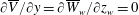 $\unicode[STIX]{x2202}\overline{V}/\unicode[STIX]{x2202}y=\unicode[STIX]{x2202}\overline{W}_{w}/\unicode[STIX]{x2202}z_{w}=0$
and replacing the
$\unicode[STIX]{x2202}\overline{V}/\unicode[STIX]{x2202}y=\unicode[STIX]{x2202}\overline{W}_{w}/\unicode[STIX]{x2202}z_{w}=0$
and replacing the
 $\unicode[STIX]{x2202}\overline{V}/\unicode[STIX]{x2202}y$
field by
$\unicode[STIX]{x2202}\overline{V}/\unicode[STIX]{x2202}y$
field by
 $-\unicode[STIX]{x2202}\overline{W}_{w}/\unicode[STIX]{x2202}z_{w}$
, the growth rate changed by
$-\unicode[STIX]{x2202}\overline{W}_{w}/\unicode[STIX]{x2202}z_{w}$
, the growth rate changed by
 $-0.0142$
and 0.0018 units of
$-0.0142$
and 0.0018 units of
 $\overline{U}_{e}/\unicode[STIX]{x1D706}_{r}$
, respectively. The former change lies within the error bound indicated by the
$\overline{U}_{e}/\unicode[STIX]{x1D706}_{r}$
, respectively. The former change lies within the error bound indicated by the
 $2\unicode[STIX]{x1D70E}$
uncertainty specified in table 2 for
$2\unicode[STIX]{x1D70E}$
uncertainty specified in table 2 for
 $N_{fr}=500$
. The latter destabilizing change is qualitatively consistent with the comparison of the
$N_{fr}=500$
. The latter destabilizing change is qualitatively consistent with the comparison of the
 $w_{v}$
- and
$w_{v}$
- and
 $v_{v}$
–
$v_{v}$
–
 $w_{v}$
-fixed approaches of Bonfigli & Kloker (Reference Bonfigli and Kloker2007, cf. figure 15(a)).
$w_{v}$
-fixed approaches of Bonfigli & Kloker (Reference Bonfigli and Kloker2007, cf. figure 15(a)).
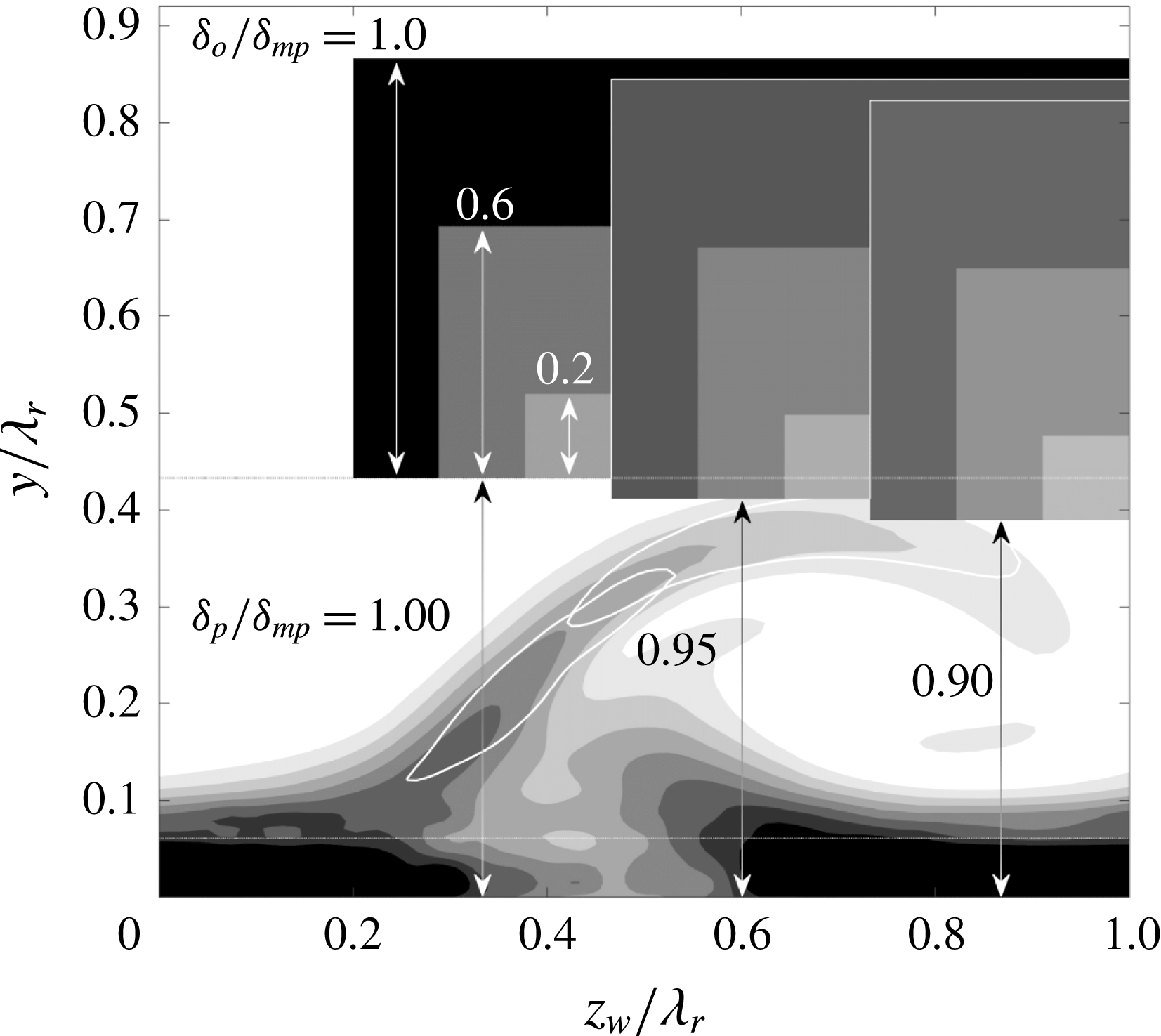
Figure 18. Overlap region definition and variations. In-plane
 $\overline{U}_{w}$
-shear magnitude of the strong vortex for
$\overline{U}_{w}$
-shear magnitude of the strong vortex for
 $N_{fr}=500$
(8 filled contours from 0 to 7 in
$N_{fr}=500$
(8 filled contours from 0 to 7 in
 $\overline{U}_{e}/\unicode[STIX]{x1D706}_{r}$
-units).
$\overline{U}_{e}/\unicode[STIX]{x1D706}_{r}$
-units).
 $|\tilde{u} _{w}|/\max |\tilde{u} _{w}|=0.5$
for most unstable type I and II modes (white contours). Near-wall region (
$|\tilde{u} _{w}|/\max |\tilde{u} _{w}|=0.5$
for most unstable type I and II modes (white contours). Near-wall region (
 $y/\unicode[STIX]{x1D706}_{r}\leqslant 0.061$
) and upper limit PIV domain (
$y/\unicode[STIX]{x1D706}_{r}\leqslant 0.061$
) and upper limit PIV domain (
 $y/\unicode[STIX]{x1D706}_{r}=0.433$
) (dotted lines).
$y/\unicode[STIX]{x1D706}_{r}=0.433$
) (dotted lines).
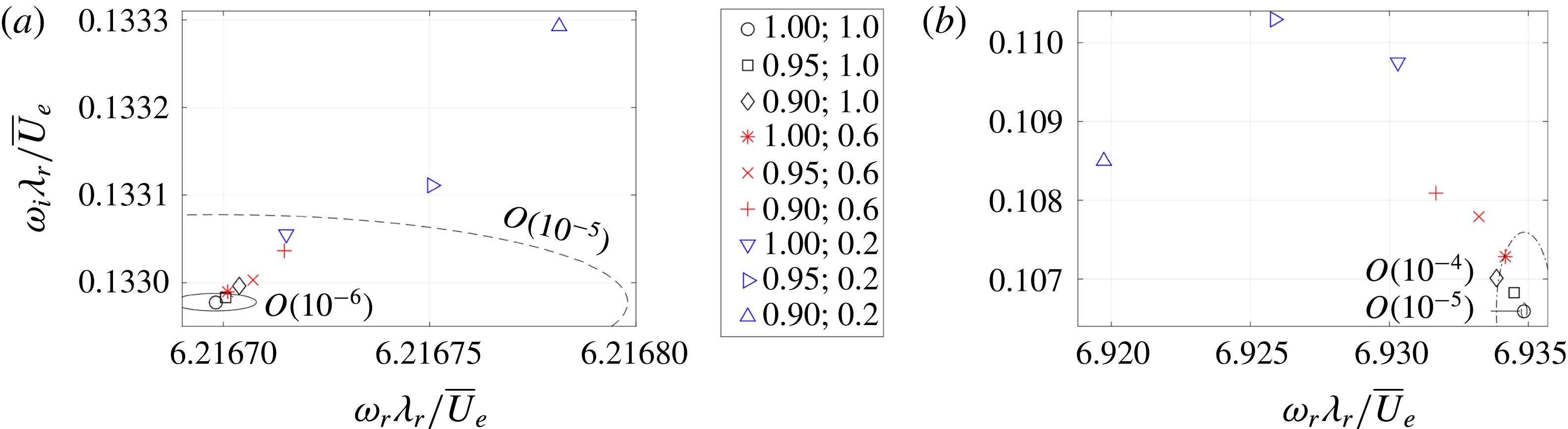
Figure 19. Type I (a) and II (b) eigenvalues (
 $\unicode[STIX]{x1D6FC}\unicode[STIX]{x1D706}_{r}=8.2$
) for different domain extrapolation parameters (legend indicates
$\unicode[STIX]{x1D6FC}\unicode[STIX]{x1D706}_{r}=8.2$
) for different domain extrapolation parameters (legend indicates
 $\unicode[STIX]{x1D6FF}_{p}$
;
$\unicode[STIX]{x1D6FF}_{p}$
;
 $\unicode[STIX]{x1D6FF}_{o}$
in units of
$\unicode[STIX]{x1D6FF}_{o}$
in units of
 $\unicode[STIX]{x1D6FF}_{mp}$
):
$\unicode[STIX]{x1D6FF}_{mp}$
):
 $10^{-6}$
(solid line),
$10^{-6}$
(solid line),
 $10^{-5}$
(dashed) and
$10^{-5}$
(dashed) and
 $10^{-4}$
(dash-dotted) neighbourhoods of the eigenvalues with
$10^{-4}$
(dash-dotted) neighbourhoods of the eigenvalues with
 $\unicode[STIX]{x1D6FF}_{p}=\unicode[STIX]{x1D6FF}_{o}=\unicode[STIX]{x1D6FF}_{mp}$
.
$\unicode[STIX]{x1D6FF}_{p}=\unicode[STIX]{x1D6FF}_{o}=\unicode[STIX]{x1D6FF}_{mp}$
.
4.4 Effect of wall-normal extrapolation
Another question related to the use of the measured mean flow is what impact the free-stream PIV data extrapolation method has on the results. Specifically, the effect of the overlap region’s parameters is to be quantified. To this end, tests were performed applying significant variations in its position, through
 $\unicode[STIX]{x1D6FF}_{p}$
, and size, with
$\unicode[STIX]{x1D6FF}_{p}$
, and size, with
 $\unicode[STIX]{x1D6FF}_{o}$
, see figure 2 for their definition. The largest value for
$\unicode[STIX]{x1D6FF}_{o}$
, see figure 2 for their definition. The largest value for
 $\unicode[STIX]{x1D6FF}_{p}$
is the height of the PIV domain,
$\unicode[STIX]{x1D6FF}_{p}$
is the height of the PIV domain,
 $\unicode[STIX]{x1D6FF}_{mp}=0.433\unicode[STIX]{x1D706}_{r}$
. By setting
$\unicode[STIX]{x1D6FF}_{mp}=0.433\unicode[STIX]{x1D706}_{r}$
. By setting
 $\unicode[STIX]{x1D6FF}_{p}<\unicode[STIX]{x1D6FF}_{mp}$
, the upper part of the PIV data are artificially altered, which is to be avoided. By increasing
$\unicode[STIX]{x1D6FF}_{p}<\unicode[STIX]{x1D6FF}_{mp}$
, the upper part of the PIV data are artificially altered, which is to be avoided. By increasing
 $\unicode[STIX]{x1D6FF}_{o}$
, the shear caused by the discontinuity is reduced. Increasing both parameters
$\unicode[STIX]{x1D6FF}_{o}$
, the shear caused by the discontinuity is reduced. Increasing both parameters
 $\unicode[STIX]{x1D6FF}_{p}$
and
$\unicode[STIX]{x1D6FF}_{p}$
and
 $\unicode[STIX]{x1D6FF}_{o}$
should therefore yield converging eigenvalues.
$\unicode[STIX]{x1D6FF}_{o}$
should therefore yield converging eigenvalues.
To test this, a
 $(\unicode[STIX]{x1D6FF}_{p},\unicode[STIX]{x1D6FF}_{o})$
-test matrix was set up, setting
$(\unicode[STIX]{x1D6FF}_{p},\unicode[STIX]{x1D6FF}_{o})$
-test matrix was set up, setting
 $\unicode[STIX]{x1D6FF}_{p}/\unicode[STIX]{x1D6FF}_{mp}=0.9$
, 0.95 and 1 and
$\unicode[STIX]{x1D6FF}_{p}/\unicode[STIX]{x1D6FF}_{mp}=0.9$
, 0.95 and 1 and
 $\unicode[STIX]{x1D6FF}_{o}/\unicode[STIX]{x1D6FF}_{mp}=0.2$
, 0.6 and 1, see figure 18. For
$\unicode[STIX]{x1D6FF}_{o}/\unicode[STIX]{x1D6FF}_{mp}=0.2$
, 0.6 and 1, see figure 18. For
 $\unicode[STIX]{x1D6FF}_{p}=0.90\unicode[STIX]{x1D6FF}_{mp}$
the type II mode is covered significantly and
$\unicode[STIX]{x1D6FF}_{p}=0.90\unicode[STIX]{x1D6FF}_{mp}$
the type II mode is covered significantly and
 $\unicode[STIX]{x1D6FF}_{o}=0.2\unicode[STIX]{x1D6FF}_{mp}$
is comparable to the vorticity thickness of the shear layer, which is expected to influence the results significantly.
$\unicode[STIX]{x1D6FF}_{o}=0.2\unicode[STIX]{x1D6FF}_{mp}$
is comparable to the vorticity thickness of the shear layer, which is expected to influence the results significantly.
The eigenvalue problem was solved, fixing
 $\unicode[STIX]{x1D6FC}\unicode[STIX]{x1D706}_{r}=8.2$
and using the
$\unicode[STIX]{x1D6FC}\unicode[STIX]{x1D706}_{r}=8.2$
and using the
 $55\times 55$
grid resolution on the
$55\times 55$
grid resolution on the
 $N_{fr}=500$
mean flow. Figure 19 shows the resulting eigenvalues. Both modes converge as
$N_{fr}=500$
mean flow. Figure 19 shows the resulting eigenvalues. Both modes converge as
 $\unicode[STIX]{x1D6FF}_{p}$
and
$\unicode[STIX]{x1D6FF}_{p}$
and
 $\unicode[STIX]{x1D6FF}_{o}$
are increased. As expected, the type II mode is affected more than type I, but the absolute eigenvalue errors are smaller than the discretization error. This is attributed to the small eigenfunction magnitudes in the overlap region. It is concluded that, when taking
$\unicode[STIX]{x1D6FF}_{o}$
are increased. As expected, the type II mode is affected more than type I, but the absolute eigenvalue errors are smaller than the discretization error. This is attributed to the small eigenfunction magnitudes in the overlap region. It is concluded that, when taking
 $\unicode[STIX]{x1D6FF}_{p}=\unicode[STIX]{x1D6FF}_{o}=0.433\unicode[STIX]{x1D706}_{r}$
, the base flow extrapolation influences the results negligibly. Table 2 reports the errors for
$\unicode[STIX]{x1D6FF}_{p}=\unicode[STIX]{x1D6FF}_{o}=0.433\unicode[STIX]{x1D706}_{r}$
, the base flow extrapolation influences the results negligibly. Table 2 reports the errors for
 $(\unicode[STIX]{x1D6FF}_{p},\unicode[STIX]{x1D6FF}_{o})/\unicode[STIX]{x1D6FF}_{mp}=(0.95,1.0)$
and
$(\unicode[STIX]{x1D6FF}_{p},\unicode[STIX]{x1D6FF}_{o})/\unicode[STIX]{x1D6FF}_{mp}=(0.95,1.0)$
and
 $(1.00,0.6)$
. These results justify using the Blasius profile for the extrapolation.
$(1.00,0.6)$
. These results justify using the Blasius profile for the extrapolation.
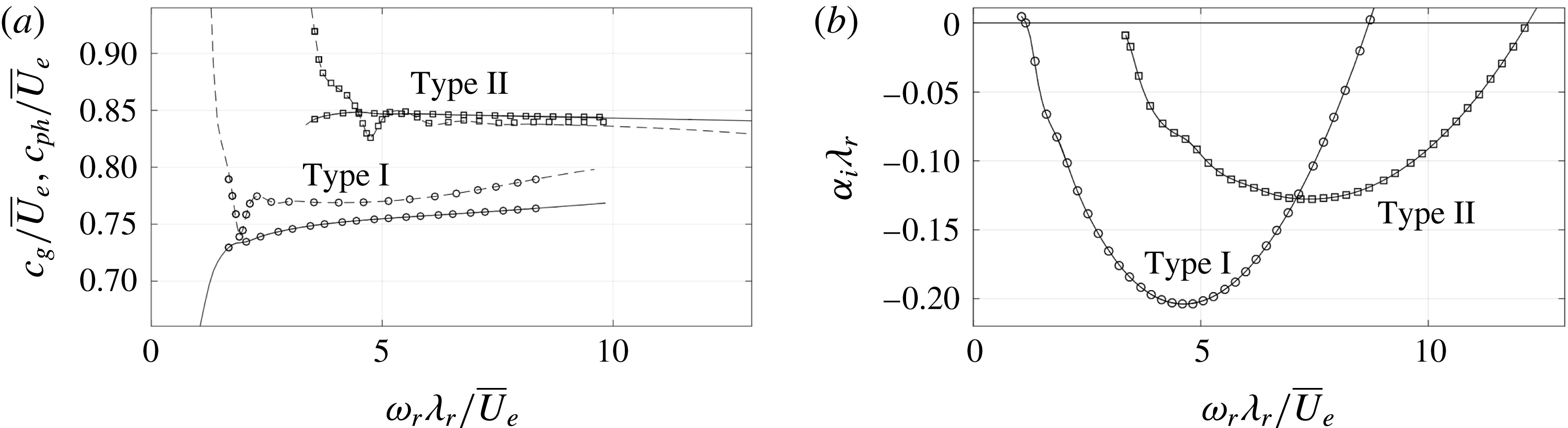
Figure 20. (a) Group (dashed lines) and phase (solid lines) speeds for both modes:
 $55\times 55$
(lines) and
$55\times 55$
(lines) and
 $90\times 90$
(symbols) grid resolution. (b) Gaster transformed temporal amplification rates,
$90\times 90$
(symbols) grid resolution. (b) Gaster transformed temporal amplification rates,
 $-\unicode[STIX]{x1D714}_{i}/c_{g}$
, (solid, solving (3.9),
$-\unicode[STIX]{x1D714}_{i}/c_{g}$
, (solid, solving (3.9),
 $\unicode[STIX]{x1D6FC}\in \mathbb{R}$
) and spatial growth rates,
$\unicode[STIX]{x1D6FC}\in \mathbb{R}$
) and spatial growth rates,
 $\unicode[STIX]{x1D6FC}_{i}$
, (symbols, solving (3.10),
$\unicode[STIX]{x1D6FC}_{i}$
, (symbols, solving (3.10),
 $\unicode[STIX]{x1D714}\in \mathbb{R}$
).
$\unicode[STIX]{x1D714}\in \mathbb{R}$
).
4.5 Applicability of the Gaster transformation
The secondary vortices are known to be convective instabilities (Bonfigli & Kloker Reference Bonfigli and Kloker2007). They grow in space subject to an imposed frequency, which corresponds to the case where
 $\unicode[STIX]{x1D6FC}\in \mathbb{C}$
is unknown and
$\unicode[STIX]{x1D6FC}\in \mathbb{C}$
is unknown and
 $\unicode[STIX]{x1D714}\in \mathbb{R}$
is given; i.e. the spatial problem. Up to now, only the solutions of the temporal problem have been handled. Equation (3.10) illustrates that the spatial stability problem is twice as expensive, because
$\unicode[STIX]{x1D714}\in \mathbb{R}$
is given; i.e. the spatial problem. Up to now, only the solutions of the temporal problem have been handled. Equation (3.10) illustrates that the spatial stability problem is twice as expensive, because
 $\unicode[STIX]{x1D6FC}$
appears quadratically in the equations. Solving this problem can be circumvented by applying the Gaster transformation, see Gaster (Reference Gaster1962), based on the fact that spatial and temporal growth are inter-related for convective perturbations. To this end, the simple formula:
$\unicode[STIX]{x1D6FC}$
appears quadratically in the equations. Solving this problem can be circumvented by applying the Gaster transformation, see Gaster (Reference Gaster1962), based on the fact that spatial and temporal growth are inter-related for convective perturbations. To this end, the simple formula:
 $$\begin{eqnarray}\displaystyle & \displaystyle \unicode[STIX]{x1D6FC}_{i}|_{\unicode[STIX]{x1D714}_{i}=0}=c_{g}^{-1}\unicode[STIX]{x1D714}_{i}|_{\unicode[STIX]{x1D6FC}_{i}=0}+O(\unicode[STIX]{x1D714}_{i}|_{\unicode[STIX]{x1D6FC}_{i}=0}^{2}), & \displaystyle\end{eqnarray}$$
can be used, where
 $c_{g}$
is the group speed shown in figure 20(a) for both mode types and compared to the phase speeds. The Gaster transformation is valid for small
$c_{g}$
is the group speed shown in figure 20(a) for both mode types and compared to the phase speeds. The Gaster transformation is valid for small
 $\unicode[STIX]{x1D714}_{i}$
-values only, see Gaster (Reference Gaster1962). The inviscid instabilities considered here have relatively large
$\unicode[STIX]{x1D714}_{i}$
-values only, see Gaster (Reference Gaster1962). The inviscid instabilities considered here have relatively large
 $\unicode[STIX]{x1D714}_{i}$
, which renders its application questionable. Nevertheless, it is well established in the literature that the transformation yields near-exact results in this case, see Malik et al. (Reference Malik, Li, Choudhari and Chang1999) and Koch et al. (Reference Koch, Bertolotti, Stolte and Hein2000). Here, this check is reproduced to rule out different sensitivities of the spatial and temporal stability problems to measurement noise in the modified base flow. Furthermore, the difference is regarded from the point of view of the eigenfunctions and the Reynolds–Orr decompositions of the eigenvalues.
$\unicode[STIX]{x1D714}_{i}$
, which renders its application questionable. Nevertheless, it is well established in the literature that the transformation yields near-exact results in this case, see Malik et al. (Reference Malik, Li, Choudhari and Chang1999) and Koch et al. (Reference Koch, Bertolotti, Stolte and Hein2000). Here, this check is reproduced to rule out different sensitivities of the spatial and temporal stability problems to measurement noise in the modified base flow. Furthermore, the difference is regarded from the point of view of the eigenfunctions and the Reynolds–Orr decompositions of the eigenvalues.
The comparison between the spatial amplification rates, obtained by solving (3.10), and the Gaster transformed temporal growth rates, obtained by solving (3.9) and applying equation (4.1), are shown in figure 20(b), using the
 $55\times 55$
grid on the
$55\times 55$
grid on the
 $N_{fr}=500$
mean flow at
$N_{fr}=500$
mean flow at
 $45.6\,\%$
chord. The eigenvalue error at the most unstable frequencies is
$45.6\,\%$
chord. The eigenvalue error at the most unstable frequencies is
 $O(10^{-4})$
; which is in line with the grid resolution accuracy. Thus, next to the agreement with the literature, the spatial and temporal problems do not display a relative sensitivity to the used measured flow field.
$O(10^{-4})$
; which is in line with the grid resolution accuracy. Thus, next to the agreement with the literature, the spatial and temporal problems do not display a relative sensitivity to the used measured flow field.
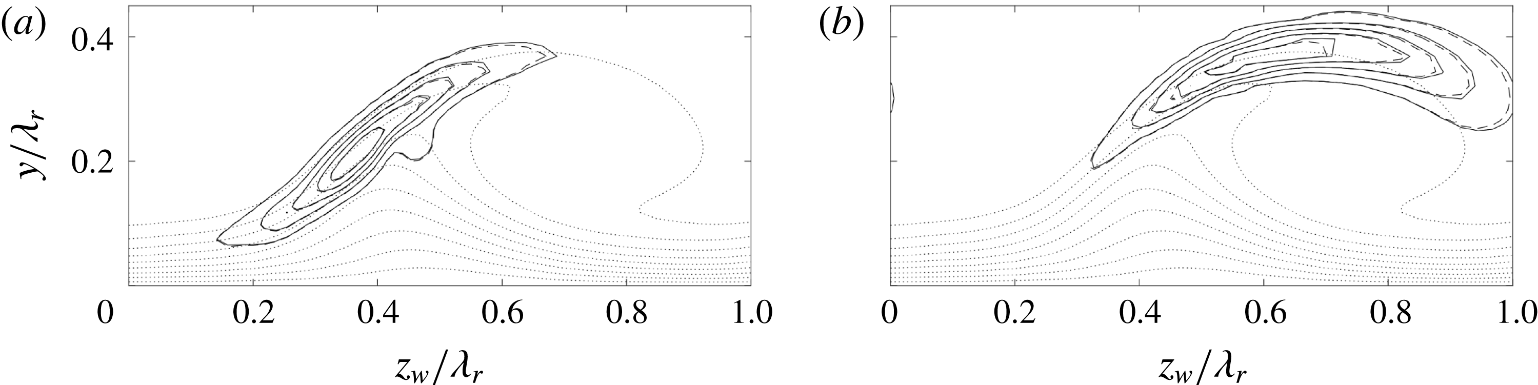
Figure 21. Temporal (solid lines,
 $\unicode[STIX]{x1D6FC}\in \mathbb{R}$
) and spatial (dashed lines,
$\unicode[STIX]{x1D6FC}\in \mathbb{R}$
) and spatial (dashed lines,
 $\unicode[STIX]{x1D714}\in \mathbb{R}$
) eigenfunctions (
$\unicode[STIX]{x1D714}\in \mathbb{R}$
) eigenfunctions (
 $|\tilde{u} _{w}|/\max |\tilde{u} _{w}|$
levels span
$|\tilde{u} _{w}|/\max |\tilde{u} _{w}|$
levels span
 $[1/6,5/6]$
with
$[1/6,5/6]$
with
 $\unicode[STIX]{x1D6E5}=1/6$
) for type I (a,
$\unicode[STIX]{x1D6E5}=1/6$
) for type I (a,
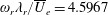 $\unicode[STIX]{x1D714}_{r}\unicode[STIX]{x1D706}_{r}/\overline{U}_{e}=4.5967$
) and II (b,
$\unicode[STIX]{x1D714}_{r}\unicode[STIX]{x1D706}_{r}/\overline{U}_{e}=4.5967$
) and II (b,
 $\unicode[STIX]{x1D714}_{r}\unicode[STIX]{x1D706}_{r}/\overline{U}_{e}=7.354$
).
$\unicode[STIX]{x1D714}_{r}\unicode[STIX]{x1D706}_{r}/\overline{U}_{e}=7.354$
).
 $\overline{U}_{w}/\overline{U}_{e}$
levels
$\overline{U}_{w}/\overline{U}_{e}$
levels
 $0.1,0.2,\ldots ,0.9$
(dotted).
$0.1,0.2,\ldots ,0.9$
(dotted).
Figure 22. (a,c)
 $\unicode[STIX]{x1D714}_{r}$
- and (b,d)
$\unicode[STIX]{x1D714}_{r}$
- and (b,d)
 $\unicode[STIX]{x1D714}_{i}$
-budgets (bars) of type I (a,b) and II (c,d), complex conjugate eigenvalue (dashed line). Temporal (top bar,
$\unicode[STIX]{x1D714}_{i}$
-budgets (bars) of type I (a,b) and II (c,d), complex conjugate eigenvalue (dashed line). Temporal (top bar,
 $\unicode[STIX]{x1D6FC}\in \mathbb{R}$
) and spatial (bottom bar,
$\unicode[STIX]{x1D6FC}\in \mathbb{R}$
) and spatial (bottom bar,
 $\unicode[STIX]{x1D714}\in \mathbb{R}$
) problem.
$\unicode[STIX]{x1D714}\in \mathbb{R}$
) problem.
Although the eigenvalues are virtually identical, this does not warrant similarity of the eigenfunctions or
 $\unicode[STIX]{x1D714}$
-budgets. Both features are compared in figures 21 and 22 for the most temporally unstable type I and II modes. It is to be noted that the most amplified modes (maximal
$\unicode[STIX]{x1D714}$
-budgets. Both features are compared in figures 21 and 22 for the most temporally unstable type I and II modes. It is to be noted that the most amplified modes (maximal
 $\unicode[STIX]{x1D6FC}_{i}$
) have a slightly lower frequency than the most unstable modes (maximal
$\unicode[STIX]{x1D6FC}_{i}$
) have a slightly lower frequency than the most unstable modes (maximal
 $\unicode[STIX]{x1D714}_{i}$
). The spatial and temporal eigenfunctions match closely, the only difference is the slightly larger extent of the temporal eigenfunction. Additionally, the phase distribution, accounting for the direction reversal, is found to be identical.
$\unicode[STIX]{x1D714}_{i}$
). The spatial and temporal eigenfunctions match closely, the only difference is the slightly larger extent of the temporal eigenfunction. Additionally, the phase distribution, accounting for the direction reversal, is found to be identical.
The
 $\unicode[STIX]{x1D714}$
-budgets are the same qualitatively, but individual terms show noticeable changes. A new contribution is that of
$\unicode[STIX]{x1D714}$
-budgets are the same qualitatively, but individual terms show noticeable changes. A new contribution is that of
 $\unicode[STIX]{x1D6FC}\overline{U}_{w}$
to
$\unicode[STIX]{x1D6FC}\overline{U}_{w}$
to
 $\unicode[STIX]{x1D714}_{i}$
. The contribution due to the
$\unicode[STIX]{x1D714}_{i}$
. The contribution due to the
 $2\unicode[STIX]{x1D6FC}_{i}\tilde{u} ^{\ast }\tilde{p}$
-term is negligible; the double integral over
$2\unicode[STIX]{x1D6FC}_{i}\tilde{u} ^{\ast }\tilde{p}$
-term is negligible; the double integral over
 $\tilde{u} ^{\ast }\tilde{p}$
evaluates to (numerical) zero. For this particular case, the changes in the individual contributions for the type I mode cancel, to yield
$\tilde{u} ^{\ast }\tilde{p}$
evaluates to (numerical) zero. For this particular case, the changes in the individual contributions for the type I mode cancel, to yield
 $-\unicode[STIX]{x1D714}_{i}\approx \unicode[STIX]{x1D6FC}_{i}\iint \overline{U}_{w}\,\tilde{\boldsymbol{q}}^{\ast }\boldsymbol{\cdot }\tilde{\boldsymbol{q}}\,\text{d}y\,\text{d}z_{w}/||\tilde{\boldsymbol{q}}||^{2}$
. This is not the case in general, shown by the type II case. The variation in the individual contributions adds up to the difference between the
$-\unicode[STIX]{x1D714}_{i}\approx \unicode[STIX]{x1D6FC}_{i}\iint \overline{U}_{w}\,\tilde{\boldsymbol{q}}^{\ast }\boldsymbol{\cdot }\tilde{\boldsymbol{q}}\,\text{d}y\,\text{d}z_{w}/||\tilde{\boldsymbol{q}}||^{2}$
. This is not the case in general, shown by the type II case. The variation in the individual contributions adds up to the difference between the
 $-\unicode[STIX]{x1D714}_{i}$
, indicated by the dashed line, and
$-\unicode[STIX]{x1D714}_{i}$
, indicated by the dashed line, and
 $\unicode[STIX]{x1D6FC}\overline{U}_{w}$
-terms. For the type I mode, this difference turns out to be small. The dominant advection terms in the
$\unicode[STIX]{x1D6FC}\overline{U}_{w}$
-terms. For the type I mode, this difference turns out to be small. The dominant advection terms in the
 $\unicode[STIX]{x1D714}_{i}$
-budget change negligibly, which is expected given the similar eigenfunctions.
$\unicode[STIX]{x1D714}_{i}$
-budget change negligibly, which is expected given the similar eigenfunctions.
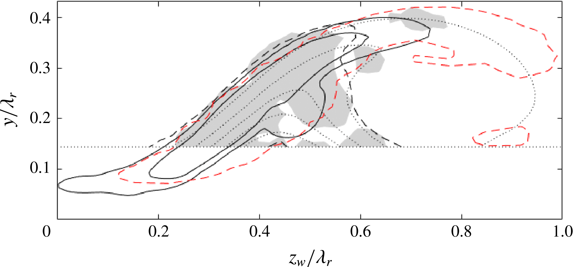
Figure 23. Velocity fluctuation fields associated with the eigenmode (solid contours,
 $|\tilde{u} _{w}|$
, levels:
$|\tilde{u} _{w}|$
, levels:
 $6.67\,\%$
and
$6.67\,\%$
and
 $20\,\%$
), the tomo-PIV total r.m.s. (dashed,
$20\,\%$
), the tomo-PIV total r.m.s. (dashed,
 $x_{w}$
-component at
$x_{w}$
-component at
 $x_{w}=15.76~\text{mm}$
, level:
$x_{w}=15.76~\text{mm}$
, level:
 $33.3\,\%$
) and the temporal r.m.s. of the POD mode couple (filled,
$33.3\,\%$
) and the temporal r.m.s. of the POD mode couple (filled,
 $\sqrt{\unicode[STIX]{x1D6F7}_{9}^{2}+\unicode[STIX]{x1D6F7}_{10}^{2}}$
at
$\sqrt{\unicode[STIX]{x1D6F7}_{9}^{2}+\unicode[STIX]{x1D6F7}_{10}^{2}}$
at
 $x_{w}=15.76~\text{mm}$
in Serpieri & Kotsonis (Reference Serpieri and Kotsonis2016), level:
$x_{w}=15.76~\text{mm}$
in Serpieri & Kotsonis (Reference Serpieri and Kotsonis2016), level:
 $20\,\%$
) and the hot-wire bandpass filtered fluctuation field (red dashed, effective velocity in the
$20\,\%$
) and the hot-wire bandpass filtered fluctuation field (red dashed, effective velocity in the
 $(X,y)$
-plane at
$(X,y)$
-plane at
 $x_{w}=0~\text{mm}$
, band 2 in Serpieri & Kotsonis (Reference Serpieri and Kotsonis2016), level:
$x_{w}=0~\text{mm}$
, band 2 in Serpieri & Kotsonis (Reference Serpieri and Kotsonis2016), level:
 $20\,\%$
). All percentages are relative to the in-plane maximum. Near-wall region for the tomo-PIV and
$20\,\%$
). All percentages are relative to the in-plane maximum. Near-wall region for the tomo-PIV and
 $\overline{U}_{w}/\overline{U}_{e}$
levels
$\overline{U}_{w}/\overline{U}_{e}$
levels
 $0.5,0.6,\ldots ,0.9$
at
$0.5,0.6,\ldots ,0.9$
at
 $x_{w}=15.76~\text{mm}$
(dotted lines).
$x_{w}=15.76~\text{mm}$
(dotted lines).
4.6 Comparison with experiments
A detailed account is given on the spatial structure of the type I mode by Serpieri & Kotsonis (Reference Serpieri and Kotsonis2016), through means of spectral and POD analysis. In particular, the POD analysis presented by Serpieri & Kotsonis (Reference Serpieri and Kotsonis2016) undeniably confirms the presence of the type I mode. This allows a detailed comparison with the retrieved eigenmode in terms of flow structure and spatial growth. Despite the limited temporal resolution of the tomo-PIV technique, the power of the POD method is to extract prominent wavelengths from the experimental data. Based on this, the eigenmode with the same spatial wavelength as the POD mode representing the type I secondary instability reported by Serpieri & Kotsonis (Reference Serpieri and Kotsonis2016) is considered. The wavelength is
 $\unicode[STIX]{x1D706}=4.6~\text{mm}$
, which corresponds to
$\unicode[STIX]{x1D706}=4.6~\text{mm}$
, which corresponds to
 $\unicode[STIX]{x1D6FC}\unicode[STIX]{x1D706}_{r}=2\unicode[STIX]{x03C0}\times 9\cos 40^{\circ }/4.6\approx 9.4$
. Note that this corresponds to a larger wavenumber than the locally most unstable mode reported in table 1. This is expected; the mode with the largest amplitude at a given location is usually situated closer to the neutral curve at a larger wavenumber.
$\unicode[STIX]{x1D6FC}\unicode[STIX]{x1D706}_{r}=2\unicode[STIX]{x03C0}\times 9\cos 40^{\circ }/4.6\approx 9.4$
. Note that this corresponds to a larger wavenumber than the locally most unstable mode reported in table 1. This is expected; the mode with the largest amplitude at a given location is usually situated closer to the neutral curve at a larger wavenumber.
First, a quantitative comparison with the experimentally measured in-plane amplitude distributions is discussed. Figure 23 shows the absolute amplitude of the
 $x_{w}$
-velocity component of the type I eigenmode versus both the hot-wire and tomo-PIV measurement results presented by Serpieri & Kotsonis (Reference Serpieri and Kotsonis2016). On the one hand, the eigenmode is compared against the bandpass filtered r.m.s. field associated with the type I mode frequency obtained from hot-wire measurements, see their figure 20 (top centre). The considered band corresponds to slightly higher frequencies,
$x_{w}$
-velocity component of the type I eigenmode versus both the hot-wire and tomo-PIV measurement results presented by Serpieri & Kotsonis (Reference Serpieri and Kotsonis2016). On the one hand, the eigenmode is compared against the bandpass filtered r.m.s. field associated with the type I mode frequency obtained from hot-wire measurements, see their figure 20 (top centre). The considered band corresponds to slightly higher frequencies,
 $5$
–
$5$
–
 $6~\text{kHz}$
, when compared to the frequency associated with the POD mode pair,
$6~\text{kHz}$
, when compared to the frequency associated with the POD mode pair,
 $4.6~\text{kHz}$
, see table 1. On the other hand, it is compared with the magnitude of the total r.m.s. and the POD pair associated with the type I mode obtained with the tomo-PIV measurements, see their figure 28.
$4.6~\text{kHz}$
, see table 1. On the other hand, it is compared with the magnitude of the total r.m.s. and the POD pair associated with the type I mode obtained with the tomo-PIV measurements, see their figure 28.
The hot-wire was oriented in the
 $Z$
-direction, measuring the effective velocity in the
$Z$
-direction, measuring the effective velocity in the
 $(X,y)$
-plane. The
$(X,y)$
-plane. The
 $y$
-velocity component is small, as indicated by the base flow and the eigenfunction, and
$y$
-velocity component is small, as indicated by the base flow and the eigenfunction, and
 $x_{w}$
and
$x_{w}$
and
 $X$
deviate only by
$X$
deviate only by
 $5^{\circ }$
, so the measured velocity is representative of the
$5^{\circ }$
, so the measured velocity is representative of the
 $x_{w}$
-velocity component. Furthermore, the hot-wire was traversed in the
$x_{w}$
-velocity component. Furthermore, the hot-wire was traversed in the
 $z$
-direction, the data corresponding to the 45 % chord station are here projected onto the
$z$
-direction, the data corresponding to the 45 % chord station are here projected onto the
 $z_{w}$
-coordinate.
$z_{w}$
-coordinate.
POD of the tomo-PIV measurement data gives two phases per advecting mode (shifted by
 $\unicode[STIX]{x03C0}/2$
), representing all velocity components in the entire measurement volume. Serpieri & Kotsonis (Reference Serpieri and Kotsonis2016) reported this pair as
$\unicode[STIX]{x03C0}/2$
), representing all velocity components in the entire measurement volume. Serpieri & Kotsonis (Reference Serpieri and Kotsonis2016) reported this pair as
 $\unicode[STIX]{x1D6F7}_{9}$
and
$\unicode[STIX]{x1D6F7}_{9}$
and
 $\unicode[STIX]{x1D6F7}_{10}$
; the ninth and tenth POD modes. The Euclidean sum of these modes, weighted with the variance of their respective time coefficients, yields an amplitude distribution with the least phase modulation. The total r.m.s. distribution corresponding to the tomo-PIV measurements is also considered for reference. The attention is focussed on the
$\unicode[STIX]{x1D6F7}_{10}$
; the ninth and tenth POD modes. The Euclidean sum of these modes, weighted with the variance of their respective time coefficients, yields an amplitude distribution with the least phase modulation. The total r.m.s. distribution corresponding to the tomo-PIV measurements is also considered for reference. The attention is focussed on the
 $x_{w}$
-velocity component, the symbol
$x_{w}$
-velocity component, the symbol
 $\unicode[STIX]{x1D6F7}$
will therefore be used to indicate the spatial structure of that component only. The tomo-PIV data are extracted at the location where the POD mode attains its maximum amplitude, at
$\unicode[STIX]{x1D6F7}$
will therefore be used to indicate the spatial structure of that component only. The tomo-PIV data are extracted at the location where the POD mode attains its maximum amplitude, at
 $x_{w}=15.76~\text{mm}$
. The maximum value of the total r.m.s.
$x_{w}=15.76~\text{mm}$
. The maximum value of the total r.m.s.
 $x_{w}$
-velocity component is equal to
$x_{w}$
-velocity component is equal to
 $0.10\,\overline{U}_{e}$
; the number used in the uncertainty arguments treated before.
$0.10\,\overline{U}_{e}$
; the number used in the uncertainty arguments treated before.
The shape of the
 $|\tilde{u} _{w}|$
amplitudes shows a qualitative agreement and can also be compared to the results of White & Saric (Reference White and Saric2005) and Serpieri & Kotsonis (Reference Serpieri and Kotsonis2018). The bandpass filtered r.m.s. field is found to have an overall similar spatial structure, but it displays a larger longitudinal extent at the leeward side of the primary vortex (towards
$|\tilde{u} _{w}|$
amplitudes shows a qualitative agreement and can also be compared to the results of White & Saric (Reference White and Saric2005) and Serpieri & Kotsonis (Reference Serpieri and Kotsonis2018). The bandpass filtered r.m.s. field is found to have an overall similar spatial structure, but it displays a larger longitudinal extent at the leeward side of the primary vortex (towards
 $z_{w}/\unicode[STIX]{x1D706}_{r}=1$
). The POD mode
$z_{w}/\unicode[STIX]{x1D706}_{r}=1$
). The POD mode
 $\unicode[STIX]{x1D6F7}_{9}$
has a significantly lower magnitude than
$\unicode[STIX]{x1D6F7}_{9}$
has a significantly lower magnitude than
 $\unicode[STIX]{x1D6F7}_{10}$
for
$\unicode[STIX]{x1D6F7}_{10}$
for
 $z_{w}>0.5\unicode[STIX]{x1D706}_{r}$
, consistent with the lower amplitude of the corresponding total r.m.s. distribution. This corroborates the segmented shape of the Euclidean sum of the POD modes. The total r.m.s. distribution shows perturbations are supported in a broader spanwise range under the primary vortex when considering all frequency content.
$z_{w}>0.5\unicode[STIX]{x1D706}_{r}$
, consistent with the lower amplitude of the corresponding total r.m.s. distribution. This corroborates the segmented shape of the Euclidean sum of the POD modes. The total r.m.s. distribution shows perturbations are supported in a broader spanwise range under the primary vortex when considering all frequency content.
Effectively, figure 23 demonstrates the merits of the stability analysis technique as a tool for experimental data reduction. The method is able to isolate the pertinent monochromatic eigenmodes based on the mean measurement data. Especially in the case of advanced flow diagnostic techniques such as tomo-PIV, it is very challenging to distinguish between the physical r.m.s. field of different modes as well as measurement noise. The (most unstable) eigenmodes give an indication of the most dominant frequencies and the expected spatial topology. The proposed methodology extends the information on the perturbation field and, furthermore, it enables enhancing the measurability of desired features by focusing the experimental set-up accordingly.
The shape of the eigenfunctions is found to be wavelength independent. However, the relative magnitudes of the
 $|\tilde{v}|$
and
$|\tilde{v}|$
and
 $|\tilde{w}_{w}|$
components change significantly for different wavelengths. The relative magnitudes of the velocity components of the eigenmode with the wavelength extracted from POD are in close agreement with the total r.m.s. values. The ratios of the in-plane maxima of
$|\tilde{w}_{w}|$
components change significantly for different wavelengths. The relative magnitudes of the velocity components of the eigenmode with the wavelength extracted from POD are in close agreement with the total r.m.s. values. The ratios of the in-plane maxima of
 $|\tilde{v}|$
and
$|\tilde{v}|$
and
 $|\tilde{w}_{w}|$
for the eigenmode are: 23 % and 50 %, relative to the maximum of
$|\tilde{w}_{w}|$
for the eigenmode are: 23 % and 50 %, relative to the maximum of
 $|\tilde{u} _{w}|$
. The same quantities for the total r.m.s. are: 21 % and 44 %, respectively. These maxima for the eigenmode are located at
$|\tilde{u} _{w}|$
. The same quantities for the total r.m.s. are: 21 % and 44 %, respectively. These maxima for the eigenmode are located at
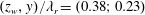 $(z_{w},y)/\unicode[STIX]{x1D706}_{r}=(0.38;0.23)$
for
$(z_{w},y)/\unicode[STIX]{x1D706}_{r}=(0.38;0.23)$
for
 $|\tilde{u} _{w}|$
and
$|\tilde{u} _{w}|$
and
 $(0.39;0.25)$
for
$(0.39;0.25)$
for
 $|\tilde{v}|$
, the total r.m.s. has both maxima at
$|\tilde{v}|$
, the total r.m.s. has both maxima at
 $(0.36,0.21)$
. The wavelength from POD is used to facilitate this specific comparison. When determined for the most unstable wavenumber reported in table 1, for example, the relative maxima of
$(0.36,0.21)$
. The wavelength from POD is used to facilitate this specific comparison. When determined for the most unstable wavenumber reported in table 1, for example, the relative maxima of
 $|\tilde{v}|$
and
$|\tilde{v}|$
and
 $|\tilde{w}_{w}|$
are 14 % and 33 %, respectively, which are lower than the values corresponding to the POD wavelength. This suggests that the mode’s wavelength can be estimated by identifying the eigenmode that has approximately the same amplitude ratios as observed in the total r.m.s. data; POD is not required for that.
$|\tilde{w}_{w}|$
are 14 % and 33 %, respectively, which are lower than the values corresponding to the POD wavelength. This suggests that the mode’s wavelength can be estimated by identifying the eigenmode that has approximately the same amplitude ratios as observed in the total r.m.s. data; POD is not required for that.
Figure 24.
 $x_{w}$
-velocity isosurfaces of (a) the type I eigenmode at
$x_{w}$
-velocity isosurfaces of (a) the type I eigenmode at
 $\unicode[STIX]{x1D714}/2\unicode[STIX]{x03C0}=4.6~\text{kHz}$
(
$\unicode[STIX]{x1D714}/2\unicode[STIX]{x03C0}=4.6~\text{kHz}$
(
 $\unicode[STIX]{x1D6FC}_{r}=9.4/\unicode[STIX]{x1D706}_{r}$
), having maximal amplitude 1 at
$\unicode[STIX]{x1D6FC}_{r}=9.4/\unicode[STIX]{x1D706}_{r}$
), having maximal amplitude 1 at
 $x=-17.6~\text{mm}$
, plotting the
$x=-17.6~\text{mm}$
, plotting the
 $\pm 84\,\%$
levels, and (b) the tomo-PIV POD mode (
$\pm 84\,\%$
levels, and (b) the tomo-PIV POD mode (
 $\unicode[STIX]{x1D6F7}_{10}$
in Serpieri & Kotsonis (Reference Serpieri and Kotsonis2016)), plotting the
$\unicode[STIX]{x1D6F7}_{10}$
in Serpieri & Kotsonis (Reference Serpieri and Kotsonis2016)), plotting the
 $\pm 0.086\overline{U}_{e}$
levels, the near-wall region is cut.
$\pm 0.086\overline{U}_{e}$
levels, the near-wall region is cut.
 $\overline{U}_{w}/\overline{U}_{e}$
levels
$\overline{U}_{w}/\overline{U}_{e}$
levels
 $0,0.05,\ldots ,1$
(contours).
$0,0.05,\ldots ,1$
(contours).
A three-dimensional representation of the eigenmode and POD mode associated with the type I instability is shown in figure 24(a) and (b), respectively, illustrating their spatial structure. The most unstable eigenmode is extrapolated in space, incorporating the exponential growth in space calculated using the Gaster transformation:
 $-\unicode[STIX]{x1D714}_{i}\unicode[STIX]{x1D706}_{r}/c_{g}=-0.09702/0.7805=-0.1243$
. These structures are compared to the 10th POD mode,
$-\unicode[STIX]{x1D714}_{i}\unicode[STIX]{x1D706}_{r}/c_{g}=-0.09702/0.7805=-0.1243$
. These structures are compared to the 10th POD mode,
 $\unicode[STIX]{x1D6F7}_{10}$
, of Serpieri & Kotsonis (Reference Serpieri and Kotsonis2016). Upstream of
$\unicode[STIX]{x1D6F7}_{10}$
, of Serpieri & Kotsonis (Reference Serpieri and Kotsonis2016). Upstream of
 $x_{w}=-4~\text{mm}$
the isosurfaces are absent in the POD mode. This is a consequence of the limited dynamic range of this particular tomo-PIV experiment and of the very low perturbation amplitude.
$x_{w}=-4~\text{mm}$
the isosurfaces are absent in the POD mode. This is a consequence of the limited dynamic range of this particular tomo-PIV experiment and of the very low perturbation amplitude.
Overall, a qualitative match of the topology is established between the modes, the largest difference being the structures’ length. Serpieri & Kotsonis (Reference Serpieri and Kotsonis2016) documented the orientation of the secondary instability structures in terms of their azimuthal angle and inclination:
 $-18.2^{\circ }$
and
$-18.2^{\circ }$
and
 $21^{\circ }$
, respectively, with respect to the stationary vortices. The eigenmode displays a comparable azimuthal angle,
$21^{\circ }$
, respectively, with respect to the stationary vortices. The eigenmode displays a comparable azimuthal angle,
 $-17.8^{\circ }$
, but a smaller inclination:
$-17.8^{\circ }$
, but a smaller inclination:
 $12^{\circ }$
. The latter angle agrees with the value reported by Janke & Balakumar (Reference Janke and Balakumar2000) and Wassermann & Kloker (Reference Wassermann and Kloker2002); who also report an inclination angle of
$12^{\circ }$
. The latter angle agrees with the value reported by Janke & Balakumar (Reference Janke and Balakumar2000) and Wassermann & Kloker (Reference Wassermann and Kloker2002); who also report an inclination angle of
 $12^{\circ }$
. A similar difference in the inclination is observed in the application to the instabilities in the wake of a micro-ramp Groot et al. (Reference Groot, Ye, van Oudheusden, Zhang and Pinna2016); the structures as observed in the tomo-PIV experiment also display a larger inclination in that case.
$12^{\circ }$
. A similar difference in the inclination is observed in the application to the instabilities in the wake of a micro-ramp Groot et al. (Reference Groot, Ye, van Oudheusden, Zhang and Pinna2016); the structures as observed in the tomo-PIV experiment also display a larger inclination in that case.
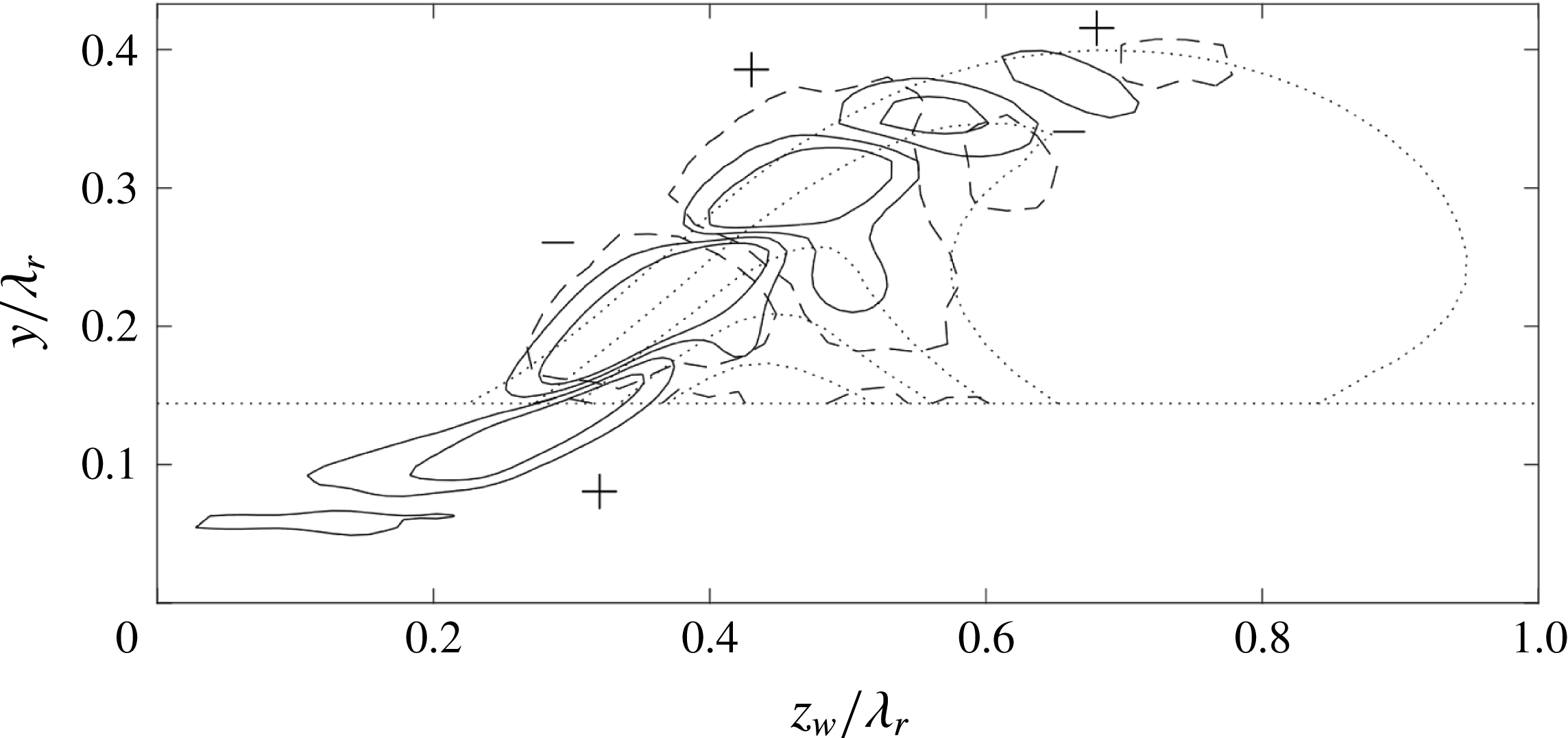
Figure 25. Eigenmode
 $\text{Re}\{\tilde{u} _{w}\}/\max |\tilde{u} _{w}|$
(solid contours) (levels:
$\text{Re}\{\tilde{u} _{w}\}/\max |\tilde{u} _{w}|$
(solid contours) (levels:
 $\pm 6.67\,\%$
and
$\pm 6.67\,\%$
and
 $\pm 20\,\%$
) and POD mode
$\pm 20\,\%$
) and POD mode
 $x_{w}$
-velocity component (
$x_{w}$
-velocity component (
 $\unicode[STIX]{x1D6F7}_{10}$
in Serpieri & Kotsonis (Reference Serpieri and Kotsonis2016)) at
$\unicode[STIX]{x1D6F7}_{10}$
in Serpieri & Kotsonis (Reference Serpieri and Kotsonis2016)) at
 $x_{w}=15.76~\text{mm}$
(dashed) (levels:
$x_{w}=15.76~\text{mm}$
(dashed) (levels:
 $\pm 20\,\%$
of in-plane maximum), level signs are indicated. Near-wall region and
$\pm 20\,\%$
of in-plane maximum), level signs are indicated. Near-wall region and
 $\overline{U}_{w}/\overline{U}_{e}$
levels
$\overline{U}_{w}/\overline{U}_{e}$
levels
 $0.5,0.6,\ldots ,0.9$
at
$0.5,0.6,\ldots ,0.9$
at
 $x_{w}=15.76~\text{mm}$
(dotted lines).
$x_{w}=15.76~\text{mm}$
(dotted lines).
The instantaneous flow structures are compared to a higher degree of detail in the
 $z_{w}y$
-plane in figure 25. The POD mode is extracted at
$z_{w}y$
-plane in figure 25. The POD mode is extracted at
 $x_{w}=15.76~\text{mm}$
, maximizing its absolute amplitude. Both modes show the same arrangement of positive and negative perturbation velocity pockets, even in locations where the velocity maxima are small, despite a slight misalignment. The orientation of the contours is the same and can be compared to phase-locked hot-wire measurement observations presented by Kawakami et al. (Reference Kawakami, Kohama and Okutsu1998) and Serpieri & Kotsonis (Reference Serpieri and Kotsonis2018) and the computations of Janke & Balakumar (Reference Janke and Balakumar2000). Two contour levels are shown for the eigenmode, of which the largest corresponds to the POD mode contour level. The lowest level shows that the structure corresponding to the POD mode is broader than the eigenmode in the direction perpendicular to the shear layer, as was already apparent in figure 24. But both modes have the same qualitative shape; both show a contour in the centre that has a large downwards protrusion. This illustrates the stability analysis effectively describes the perturbation flow topology. The broader structures observed in the measurement could be explained by the limited capability of the tomo-PIV experiment in capturing complicated flow structures in the presence of strong shear. From the perspective of the (de)stabilizing action of the in-plane advection terms in (3.7), the broader structure would be more stabilized as this corresponds to a larger white region in figure 13(c).
$x_{w}=15.76~\text{mm}$
, maximizing its absolute amplitude. Both modes show the same arrangement of positive and negative perturbation velocity pockets, even in locations where the velocity maxima are small, despite a slight misalignment. The orientation of the contours is the same and can be compared to phase-locked hot-wire measurement observations presented by Kawakami et al. (Reference Kawakami, Kohama and Okutsu1998) and Serpieri & Kotsonis (Reference Serpieri and Kotsonis2018) and the computations of Janke & Balakumar (Reference Janke and Balakumar2000). Two contour levels are shown for the eigenmode, of which the largest corresponds to the POD mode contour level. The lowest level shows that the structure corresponding to the POD mode is broader than the eigenmode in the direction perpendicular to the shear layer, as was already apparent in figure 24. But both modes have the same qualitative shape; both show a contour in the centre that has a large downwards protrusion. This illustrates the stability analysis effectively describes the perturbation flow topology. The broader structures observed in the measurement could be explained by the limited capability of the tomo-PIV experiment in capturing complicated flow structures in the presence of strong shear. From the perspective of the (de)stabilizing action of the in-plane advection terms in (3.7), the broader structure would be more stabilized as this corresponds to a larger white region in figure 13(c).
Having identified the correspondence between the structures of the eigenmode and POD mode, the exponential growth can be analysed. It should be highly stressed here that there is no reason to expect that the eigenmode and POD mode should display the same growth rate. The POD mode is a data-driven, energy-maximizing coherent structure having a broad spectral content, that is, to a degree, corrupted with systematic and random measurement noise. As stated by Serpieri & Kotsonis (Reference Serpieri and Kotsonis2016), other POD modes showed similar structures to that in figure 24 and this corroborates with the broad frequency band in the hot-wire spectrum for type I mode fluctuations. An eigenmode, on the other hand, is purely monochromatic and represents a rigorous solution of the governing equations, making it an entirely different entity. Growth rates are moreover notoriously hard to match, as pointed out with the executed sensitivity study and by verification studies in the computational literature, see Bonfigli & Kloker (Reference Bonfigli and Kloker2007). For this reason, the scope of this comparison serves more as a qualitative comparison for the methodology, rather than a strict validation.
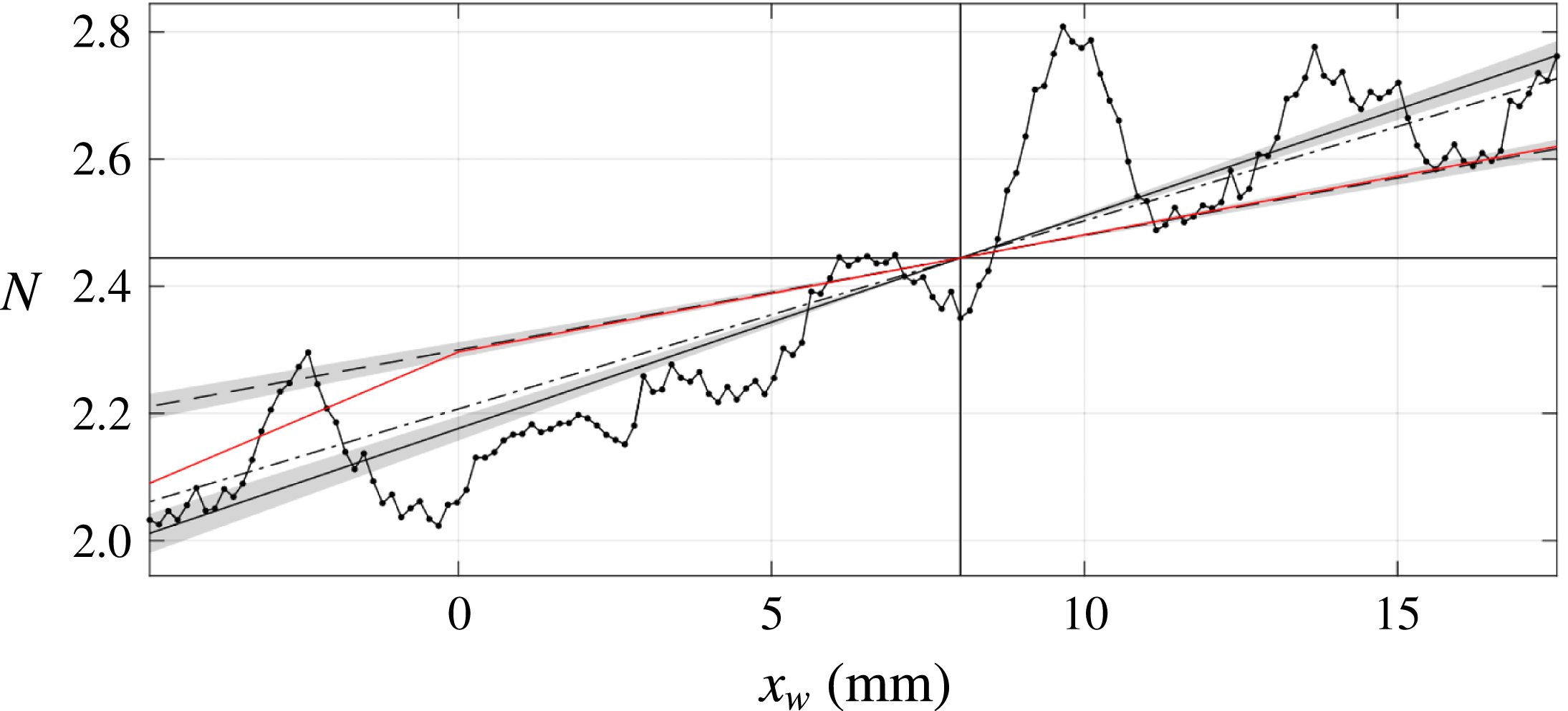
Figure 26.
 $N$
-factors based on the: POD mode couple r.m.s. (dotted line), linear fit to POD r.m.s. (solid line), bandpass filtered hot-wire anemometry velocity fluctuation fields reproduced from figure 21(b) of Serpieri & Kotsonis (Reference Serpieri and Kotsonis2016, band 2) (red), eigenmode: most unstable (dashed,
$N$
-factors based on the: POD mode couple r.m.s. (dotted line), linear fit to POD r.m.s. (solid line), bandpass filtered hot-wire anemometry velocity fluctuation fields reproduced from figure 21(b) of Serpieri & Kotsonis (Reference Serpieri and Kotsonis2016, band 2) (red), eigenmode: most unstable (dashed,
 $\unicode[STIX]{x1D6FC}\unicode[STIX]{x1D706}_{r}=6.2$
) and POD wavelength (dash-dotted,
$\unicode[STIX]{x1D6FC}\unicode[STIX]{x1D706}_{r}=6.2$
) and POD wavelength (dash-dotted,
 $9.4$
). Uncertainty in linear fit slope and growth rate based on
$9.4$
). Uncertainty in linear fit slope and growth rate based on
 $2\unicode[STIX]{x1D70E}$
in table 2 (shaded).
$2\unicode[STIX]{x1D70E}$
in table 2 (shaded).
The r.m.s. field of the coupled POD modes is integrated in both wall-normal and spanwise directions, towards producing a relative amplitude. The
 $N$
-factor is defined as the natural logarithm of the resulting quantity:
$N$
-factor is defined as the natural logarithm of the resulting quantity:
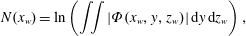 $$\begin{eqnarray}\displaystyle & \displaystyle N(x_{w})=\ln \left(\iint |\unicode[STIX]{x1D6F7}(x_{w},y,z_{w})|\;\text{d}y\,\text{d}z_{w}\right), & \displaystyle\end{eqnarray}$$
where
 $\unicode[STIX]{x1D6F7}$
corresponds to the
$\unicode[STIX]{x1D6F7}$
corresponds to the
 $x_{w}$
-velocity component of the POD mode couple. The integral can be evaluated in the
$x_{w}$
-velocity component of the POD mode couple. The integral can be evaluated in the
 $x_{w}$
-range
$x_{w}$
-range
 $[-4,17]$
in millimetres, where the dynamical range of the experiment was sufficient to resolve the mode couple. Serpieri & Kotsonis (Reference Serpieri and Kotsonis2016) reported
$[-4,17]$
in millimetres, where the dynamical range of the experiment was sufficient to resolve the mode couple. Serpieri & Kotsonis (Reference Serpieri and Kotsonis2016) reported
 $N$
-curves in their figure 21(b), based on the bandpass filtered r.m.s. data corresponding to the type I frequency range, measured using hot-wire anemometry. That figure illustrates that the former streamwise range does not include the upstream neutral point. For that reason, the currently extracted
$N$
-curves in their figure 21(b), based on the bandpass filtered r.m.s. data corresponding to the type I frequency range, measured using hot-wire anemometry. That figure illustrates that the former streamwise range does not include the upstream neutral point. For that reason, the currently extracted
 $N$
-curve is shifted to the value (
$N$
-curve is shifted to the value (
 $N=2.44$
) extracted from their results at the location currently investigated. The resulting
$N=2.44$
) extracted from their results at the location currently investigated. The resulting
 $N$
-curve is shown in figure 26. The oscillation in the dotted curve, with a wavelength comparable to the individual POD mode of
$N$
-curve is shown in figure 26. The oscillation in the dotted curve, with a wavelength comparable to the individual POD mode of
 $4.6~\text{mm}$
, reflects the underlying phase undulation of the spatial velocity maxima. A clear growth trend is obtained nonetheless. A linear fit is used to obtain a quantitative means of comparison for the eigenmode growth. The fitted slope corresponds to
$4.6~\text{mm}$
, reflects the underlying phase undulation of the spatial velocity maxima. A clear growth trend is obtained nonetheless. A linear fit is used to obtain a quantitative means of comparison for the eigenmode growth. The fitted slope corresponds to
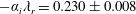 $-\unicode[STIX]{x1D6FC}_{i}\unicode[STIX]{x1D706}_{r}=0.230\pm 0.008$
. This value is significantly larger compared to the growth rate of the eigenmode with the same wavelength, for which
$-\unicode[STIX]{x1D6FC}_{i}\unicode[STIX]{x1D706}_{r}=0.230\pm 0.008$
. This value is significantly larger compared to the growth rate of the eigenmode with the same wavelength, for which
 $-\unicode[STIX]{x1D6FC}_{i}\unicode[STIX]{x1D706}_{r}=0.1243$
. This is reflected in the mismatch of the slopes of the
$-\unicode[STIX]{x1D6FC}_{i}\unicode[STIX]{x1D706}_{r}=0.1243$
. This is reflected in the mismatch of the slopes of the
 $N$
-curves in figure 26. The grey area about the
$N$
-curves in figure 26. The grey area about the
 $N$
-curve for the eigenmode indicates the uncertainty (
$N$
-curve for the eigenmode indicates the uncertainty (
 $\pm 2\unicode[STIX]{x1D70E}=\pm 0.0106$
units) given in table 2. Including the worst error estimate, the growth rate does not match that extracted from the POD mode. The
$\pm 2\unicode[STIX]{x1D70E}=\pm 0.0106$
units) given in table 2. Including the worst error estimate, the growth rate does not match that extracted from the POD mode. The
 $N$
-curve corresponding to the most unstable eigenmode is also included, for which
$N$
-curve corresponding to the most unstable eigenmode is also included, for which
 $-\unicode[STIX]{x1D6FC}_{i}\unicode[STIX]{x1D706}_{r}=0.2041$
. This value only slightly underestimates the value corresponding to the POD mode.
$-\unicode[STIX]{x1D6FC}_{i}\unicode[STIX]{x1D706}_{r}=0.2041$
. This value only slightly underestimates the value corresponding to the POD mode.
The
 $N$
-curve corresponding to the bandpass filtered fluctuation field associated with the type I mode (band 2) shown in figure 21(b) of Serpieri & Kotsonis (Reference Serpieri and Kotsonis2016), corresponding to hot-wire measurements of the same vortices, is repeated here. This curve reflects the growth rate
$N$
-curve corresponding to the bandpass filtered fluctuation field associated with the type I mode (band 2) shown in figure 21(b) of Serpieri & Kotsonis (Reference Serpieri and Kotsonis2016), corresponding to hot-wire measurements of the same vortices, is repeated here. This curve reflects the growth rate
 $-\unicode[STIX]{x1D6FC}_{i}\unicode[STIX]{x1D706}_{r}=0.1270$
, including the projection onto the
$-\unicode[STIX]{x1D6FC}_{i}\unicode[STIX]{x1D706}_{r}=0.1270$
, including the projection onto the
 $x_{w}$
-direction (uncorrected value:
$x_{w}$
-direction (uncorrected value:
 $0.1272$
), which does match the considered eigenmode’s growth to within the uncertainty. The latter match should, however, be interpreted with caution. The experimental curve corresponds to the r.m.s. amplitude averaged over 3 neighbouring vortices, amongst which are both the currently investigated ones, and the curve has a sample spacing of 0.025 % chord, corresponding to
$0.1272$
), which does match the considered eigenmode’s growth to within the uncertainty. The latter match should, however, be interpreted with caution. The experimental curve corresponds to the r.m.s. amplitude averaged over 3 neighbouring vortices, amongst which are both the currently investigated ones, and the curve has a sample spacing of 0.025 % chord, corresponding to
 $29~\text{mm}$
in the
$29~\text{mm}$
in the
 $x_{w}$
-coordinate. In summary, qualitative agreement between the stability analysis and experimental measurements further demonstrates the applicability of the proposed methodology towards enhancing and extending the experimental measurability.
$x_{w}$
-coordinate. In summary, qualitative agreement between the stability analysis and experimental measurements further demonstrates the applicability of the proposed methodology towards enhancing and extending the experimental measurability.
4.7 Effect of primary vortex strength
As mentioned in § 2.3, two neighbouring vortices are measured, where the left-hand side vortex is slightly weaker (27.3 %
 $\overline{U}_{e}$
) than the right-hand side vortex (28.7 %
$\overline{U}_{e}$
) than the right-hand side vortex (28.7 %
 $\overline{U}_{e}$
) considered up to now. Next to the reduced strength, the perturbations have been experimentally identified to be much weaker by using the POD technique in the vicinity of the weak vortex, suggesting that the lower primary amplitude results in a reduced growth of the secondary instability modes.
$\overline{U}_{e}$
) considered up to now. Next to the reduced strength, the perturbations have been experimentally identified to be much weaker by using the POD technique in the vicinity of the weak vortex, suggesting that the lower primary amplitude results in a reduced growth of the secondary instability modes.
The mild difference in amplitude between the primary crossflow vortices provides an ideal case in demonstrating the ability of the global stability approach to identify pertinent stability features based on the measured mean flow alone. The analysis performed so far on the baseline stronger vortex is here repeated for the weaker vortex using the domain
 $-1\leqslant z_{w}/\unicode[STIX]{x1D706}_{r}\leqslant 0$
indicated in figure 3 and a mean field constructed with 500 instantaneous snapshots. For ease of comparison purposes, the domain is translated in the
$-1\leqslant z_{w}/\unicode[STIX]{x1D706}_{r}\leqslant 0$
indicated in figure 3 and a mean field constructed with 500 instantaneous snapshots. For ease of comparison purposes, the domain is translated in the
 $z_{w}$
-direction, so the
$z_{w}$
-direction, so the
 $z_{w}$
-coordinate again spans
$z_{w}$
-coordinate again spans
 $[0,\unicode[STIX]{x1D706}_{r}]$
. In figure 27, the type I and II mode branches are shown and compared with those corresponding to the stronger vortex. The branches are given for two grid resolutions. The most unstable type I and II modes are again found to be subject to
$[0,\unicode[STIX]{x1D706}_{r}]$
. In figure 27, the type I and II mode branches are shown and compared with those corresponding to the stronger vortex. The branches are given for two grid resolutions. The most unstable type I and II modes are again found to be subject to
 $O(10^{-5})$
and
$O(10^{-5})$
and
 $O(10^{-4})$
eigenvalue errors, respectively.
$O(10^{-4})$
eigenvalue errors, respectively.
Figure 27. Type I (circles) and II (squares) temporal stability branches for the weak vortex using
 $N_{z}\times N_{y}=55\times 55$
(dashed lines) and
$N_{z}\times N_{y}=55\times 55$
(dashed lines) and
 $90\times 90$
(solid) grid nodes. Strong vortex branches (solid without open symbols). Arrows link type I and II modes with
$90\times 90$
(solid) grid nodes. Strong vortex branches (solid without open symbols). Arrows link type I and II modes with
 $\unicode[STIX]{x1D6FC}\unicode[STIX]{x1D706}_{r}=6.2$
and 8.6 (filled symbols), respectively, on the different vortices. All most unstable eigenvalue symbols are filled. Eigenvalues corresponding to domain containing both strong and weak primary vortices using
$\unicode[STIX]{x1D6FC}\unicode[STIX]{x1D706}_{r}=6.2$
and 8.6 (filled symbols), respectively, on the different vortices. All most unstable eigenvalue symbols are filled. Eigenvalues corresponding to domain containing both strong and weak primary vortices using
 $N_{z}\times N_{y}=140\times 70$
(red symbols). Branches corresponding to the interpolated base flows with
$N_{z}\times N_{y}=140\times 70$
(red symbols). Branches corresponding to the interpolated base flows with
 $\unicode[STIX]{x1D712}=0.2,0.4,0.6$
and
$\unicode[STIX]{x1D712}=0.2,0.4,0.6$
and
 $0.8$
(dotted lines, bottom to top).
$0.8$
(dotted lines, bottom to top).
Despite the mild differences in the base flow, the stability characteristics of the weaker vortex are drastically changed towards a more stable state. The type I mode is stable for all wavenumbers and type II is marginally unstable, indicating the weak vortex amplitude of 27.3 %
 $\overline{U}_{e}$
based on (2.1) is close to the neutral secondary instability limit for both currently considered modes. This further corroborates the low perturbation amplitude observed in the experimental flow field. The most unstable modes’ characteristics for both vortices are compared in table 3.
$\overline{U}_{e}$
based on (2.1) is close to the neutral secondary instability limit for both currently considered modes. This further corroborates the low perturbation amplitude observed in the experimental flow field. The most unstable modes’ characteristics for both vortices are compared in table 3.
Table 3. Parameters of the most temporally unstable modes in the base spectrum corresponding to the weaker (left) and stronger (right) vortex in figure 3.
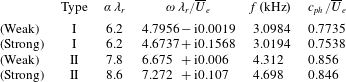
Due to the apparent extreme sensitivity of stability on the vortex strength, an order-of-magnitude check is performed by comparing the order of magnitude of the growth rates to the work of Koch et al. (Reference Koch, Bertolotti, Stolte and Hein2000) and Bonfigli & Kloker (Reference Bonfigli and Kloker2007). The current Reynolds number,
 $Re=\overline{U}_{e}\unicode[STIX]{x1D706}_{r}/\unicode[STIX]{x1D708}=1.32\times 10^{4}$
, while the latter authors’ simulations correspond to
$Re=\overline{U}_{e}\unicode[STIX]{x1D706}_{r}/\unicode[STIX]{x1D708}=1.32\times 10^{4}$
, while the latter authors’ simulations correspond to
 $1.34\times 10^{4}$
and
$1.34\times 10^{4}$
and
 $0.87\times 10^{4}$
, respectively. Assuming a comparable integral effect of the pressure gradient, the current results are comparable with those of Koch et al. (Reference Koch, Bertolotti, Stolte and Hein2000), while relatively larger shear levels and therefore growth rates are expected in the case of Bonfigli & Kloker (Reference Bonfigli and Kloker2007). By converting the maximal growth rates in these reference into
$0.87\times 10^{4}$
, respectively. Assuming a comparable integral effect of the pressure gradient, the current results are comparable with those of Koch et al. (Reference Koch, Bertolotti, Stolte and Hein2000), while relatively larger shear levels and therefore growth rates are expected in the case of Bonfigli & Kloker (Reference Bonfigli and Kloker2007). By converting the maximal growth rates in these reference into
 $\overline{U}_{e}/\unicode[STIX]{x1D706}_{r}$
units, one respectively retrieves the values 0.49 and 1.5, which, compared to the currently found maximal value of 0.16, are significantly larger. (In their nomenclature, for Koch et al. (Reference Koch, Bertolotti, Stolte and Hein2000, cf. figure 18):
$\overline{U}_{e}/\unicode[STIX]{x1D706}_{r}$
units, one respectively retrieves the values 0.49 and 1.5, which, compared to the currently found maximal value of 0.16, are significantly larger. (In their nomenclature, for Koch et al. (Reference Koch, Bertolotti, Stolte and Hein2000, cf. figure 18):
 $(\unicode[STIX]{x1D70E}_{r}L_{ref}^{\ast }/Q_{ref}^{\ast })\times (\unicode[STIX]{x1D706}_{z_{c}}^{\ast }/L_{ref}^{\ast })\times$
 $(Q_{ref}^{\ast }/Q_{e}^{\ast })=0.029\times 12/0.7092\times 1=0.49$
and for Bonfigli & Kloker (Reference Bonfigli and Kloker2007, cf. figure 13):
$(Q_{ref}^{\ast }/Q_{e}^{\ast })=0.029\times 12/0.7092\times 1=0.49$
and for Bonfigli & Kloker (Reference Bonfigli and Kloker2007, cf. figure 13):
 $(\text{Im}(\unicode[STIX]{x1D714})L_{ref}^{\ast }/u_{\infty }^{\ast })\times (\unicode[STIX]{x1D706}_{0,z}^{\ast }/L_{ref}^{\ast })\times (u_{\infty }^{\ast }/u_{b,e}^{\ast })=10\times 12/100\times 14/11=1.5.$
) Similarly, the maximal growth rate of the primary instability reported by Koch et al. (Reference Koch, Bertolotti, Stolte and Hein2000) is 0.12. This is taken as an indication that the currently considered strong vortex lingers close to neutral conditions. This is a reasonable explanation for the apparent large decrease of the growth rate of the strong, as opposed to the weak vortex. The near-neutral conditions are also reasonable in the perspective of the small difference in the vortex amplitudes.
$(\text{Im}(\unicode[STIX]{x1D714})L_{ref}^{\ast }/u_{\infty }^{\ast })\times (\unicode[STIX]{x1D706}_{0,z}^{\ast }/L_{ref}^{\ast })\times (u_{\infty }^{\ast }/u_{b,e}^{\ast })=10\times 12/100\times 14/11=1.5.$
) Similarly, the maximal growth rate of the primary instability reported by Koch et al. (Reference Koch, Bertolotti, Stolte and Hein2000) is 0.12. This is taken as an indication that the currently considered strong vortex lingers close to neutral conditions. This is a reasonable explanation for the apparent large decrease of the growth rate of the strong, as opposed to the weak vortex. The near-neutral conditions are also reasonable in the perspective of the small difference in the vortex amplitudes.
The estimate of the primary amplitude leading to neutral secondary modes of Fischer et al. (Reference Fischer, Hein and Dallmann1993) of 11 %
 $\overline{U}_{e}$
is rather low compared to the value found here. The order of magnitude is comparable with the results of Wassermann & Kloker (Reference Wassermann and Kloker2002), reporting 30 %
$\overline{U}_{e}$
is rather low compared to the value found here. The order of magnitude is comparable with the results of Wassermann & Kloker (Reference Wassermann and Kloker2002), reporting 30 %
 $\overline{U}_{e}$
based on the maximum deceleration imposed by the mean flow distortion. Instances of the type I eigenmode being more stable than type II for all wavenumbers are uncommon, e.g. see Koch et al. (Reference Koch, Bertolotti, Stolte and Hein2000). As elaborated on in § 2.3, the in-plane velocity components show a small increase relative to the primary perturbation amplitude based on
$\overline{U}_{e}$
based on the maximum deceleration imposed by the mean flow distortion. Instances of the type I eigenmode being more stable than type II for all wavenumbers are uncommon, e.g. see Koch et al. (Reference Koch, Bertolotti, Stolte and Hein2000). As elaborated on in § 2.3, the in-plane velocity components show a small increase relative to the primary perturbation amplitude based on
 $\overline{U}_{s}$
. Based on figure 20 of Bonfigli & Kloker (Reference Bonfigli and Kloker2007), this effect should render the type II mode more stable than type I.
$\overline{U}_{s}$
. Based on figure 20 of Bonfigli & Kloker (Reference Bonfigli and Kloker2007), this effect should render the type II mode more stable than type I.
For the stronger vortex, the most unstable wavenumbers for the type I and II modes are
 $\unicode[STIX]{x1D6FC}\unicode[STIX]{x1D706}_{r}=6.2$
and 8.6, respectively. The arrows in figure 27 link the modes corresponding to these wavenumbers for both vortices. Bonfigli & Kloker (Reference Bonfigli and Kloker2007) show (cf. figure 36b) the frequencies for fixed wavenumbers are proportional to the primary vortex strength, i.e. a decrease of approximately 1.4 % is expected. Instead, the frequency at a fixed wavenumber increases 2.6 % for type I and 1.2 % for type II. By inspection of the terms in the
$\unicode[STIX]{x1D6FC}\unicode[STIX]{x1D706}_{r}=6.2$
and 8.6, respectively. The arrows in figure 27 link the modes corresponding to these wavenumbers for both vortices. Bonfigli & Kloker (Reference Bonfigli and Kloker2007) show (cf. figure 36b) the frequencies for fixed wavenumbers are proportional to the primary vortex strength, i.e. a decrease of approximately 1.4 % is expected. Instead, the frequency at a fixed wavenumber increases 2.6 % for type I and 1.2 % for type II. By inspection of the terms in the
 $\unicode[STIX]{x1D714}_{r}$
-budget, the increase of the frequency for a fixed wavenumber cannot be associated with an individual term; it is the integral effect of small changes in all terms. For the type I mode,
$\unicode[STIX]{x1D714}_{r}$
-budget, the increase of the frequency for a fixed wavenumber cannot be associated with an individual term; it is the integral effect of small changes in all terms. For the type I mode,
 $\unicode[STIX]{x1D6FC}\unicode[STIX]{x1D706}_{r}=6.2$
is again most unstable. For the type II mode, the most unstable wavenumber is smaller for the weaker vortex. This behaviour for the type I mode agrees with the results of Koch et al. (Reference Koch, Bertolotti, Stolte and Hein2000), who report a type I branch (cf. figure 18) that has an invariant most unstable frequency at different streamwise locations, although that type I branch is not the most unstable type I harmonic over the considered streamwise range.
$\unicode[STIX]{x1D6FC}\unicode[STIX]{x1D706}_{r}=6.2$
is again most unstable. For the type II mode, the most unstable wavenumber is smaller for the weaker vortex. This behaviour for the type I mode agrees with the results of Koch et al. (Reference Koch, Bertolotti, Stolte and Hein2000), who report a type I branch (cf. figure 18) that has an invariant most unstable frequency at different streamwise locations, although that type I branch is not the most unstable type I harmonic over the considered streamwise range.
To further assess the reliability of the decrease in the growth rate from the strong to the weak vortex, intermediate temporal stability branches are computed based on the flow obtained by artificially interpolating the two vortices considered here. The strength parameter
 $\unicode[STIX]{x1D712}$
is introduced, defining the interpolated solution as follows:
$\unicode[STIX]{x1D712}$
is introduced, defining the interpolated solution as follows:
 $$\begin{eqnarray}\displaystyle & \displaystyle \overline{Q}_{\unicode[STIX]{x1D712}}(z_{w},y)=\unicode[STIX]{x1D712}\overline{Q}_{[0,1]}(z_{w},y)+(1-\unicode[STIX]{x1D712})\overline{Q}_{[-1,0]}(z_{w}-\unicode[STIX]{x1D706}_{r},y), & \displaystyle\end{eqnarray}$$
where
 $\overline{Q}$
denotes any mean flow variable,
$\overline{Q}$
denotes any mean flow variable,
 $\overline{Q}_{\unicode[STIX]{x1D712}}$
is the interpolated flow variable and
$\overline{Q}_{\unicode[STIX]{x1D712}}$
is the interpolated flow variable and
 $\overline{Q}_{[0,1]}$
and
$\overline{Q}_{[0,1]}$
and
 $\overline{Q}_{[-1,0]}$
denote the strong and weak vortices, respectively. A similar approach is deployed by Piot (Reference Piot2008) to investigate the effect of a bump on a boundary layer flow. The values
$\overline{Q}_{[-1,0]}$
denote the strong and weak vortices, respectively. A similar approach is deployed by Piot (Reference Piot2008) to investigate the effect of a bump on a boundary layer flow. The values
 $\unicode[STIX]{x1D712}=$
0.2, 0.4, 0.6 and 0.8 are considered and the attention is restricted to the type I mode. The results are shown as the dotted lines in figure 28. Evidently, transitioning from the strong to the weak vortex corresponds to a consistent and monotonic decrease of the branch in the
$\unicode[STIX]{x1D712}=$
0.2, 0.4, 0.6 and 0.8 are considered and the attention is restricted to the type I mode. The results are shown as the dotted lines in figure 28. Evidently, transitioning from the strong to the weak vortex corresponds to a consistent and monotonic decrease of the branch in the
 $\unicode[STIX]{x1D714}$
-plane, further confirming that the decreased growth rate is not a random artefact of the measured flow representation.
$\unicode[STIX]{x1D714}$
-plane, further confirming that the decreased growth rate is not a random artefact of the measured flow representation.
A comparison of the most unstable eigenfunctions of the different vortices is shown in figure 28. Both eigenfunctions display a broader support about the vortex. This behaviour is qualitatively comparable to the findings of Koch et al. (Reference Koch, Bertolotti, Stolte and Hein2000). Furthermore, the maxima of the functions have a higher position relative to the distorted base flow contours, which is reflected by slightly higher phase speeds, see table 3. In turn, this is directly linked to the slight increase of the frequencies at constant wavenumber discussed before. The difference in the orientation of the highest level contour of the type II mode is important to note. For the stronger vortex, this is located to the left of the primary vortex core and tilted to the left, whereas for the weaker vortex it is located and tilted to the right.
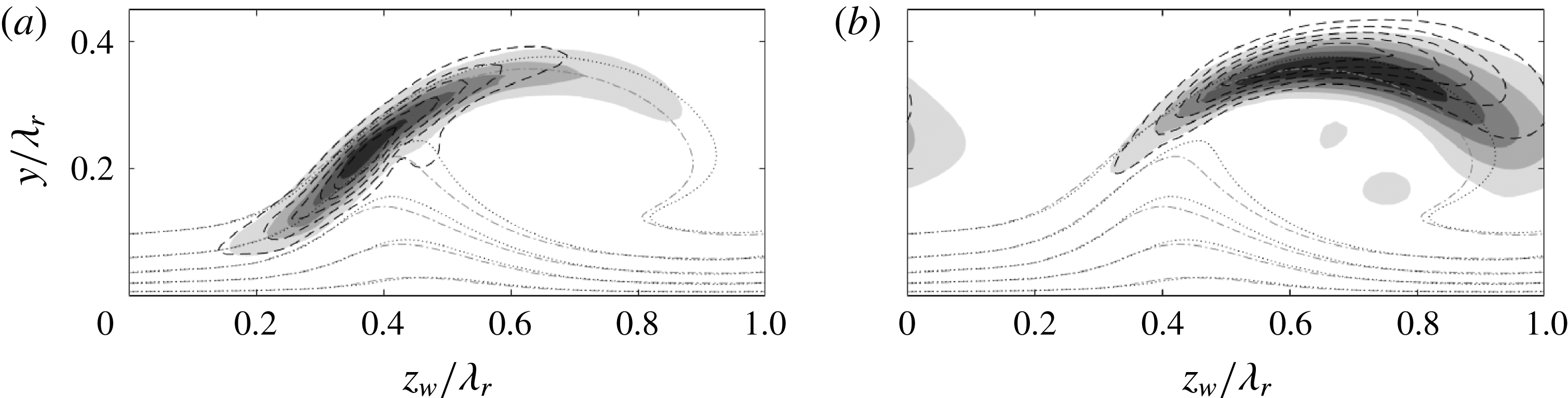
Figure 28.
 $|\tilde{u} _{w}|/\max |\tilde{u} _{w}|$
for type I (a) and II (b) (levels span
$|\tilde{u} _{w}|/\max |\tilde{u} _{w}|$
for type I (a) and II (b) (levels span
 $[1/6,5/6]$
with
$[1/6,5/6]$
with
 $\unicode[STIX]{x1D6E5}=1/6$
) for the weak (filled contours) and strong (dashed) vortex.
$\unicode[STIX]{x1D6E5}=1/6$
) for the weak (filled contours) and strong (dashed) vortex.
 $\overline{U}_{w}/\overline{U}_{e}$
levels
$\overline{U}_{w}/\overline{U}_{e}$
levels
 $0.1,0.3,\ldots ,0.9$
for the weak (dash-dotted) and strong (dotted) vortex.
$0.1,0.3,\ldots ,0.9$
for the weak (dash-dotted) and strong (dotted) vortex.
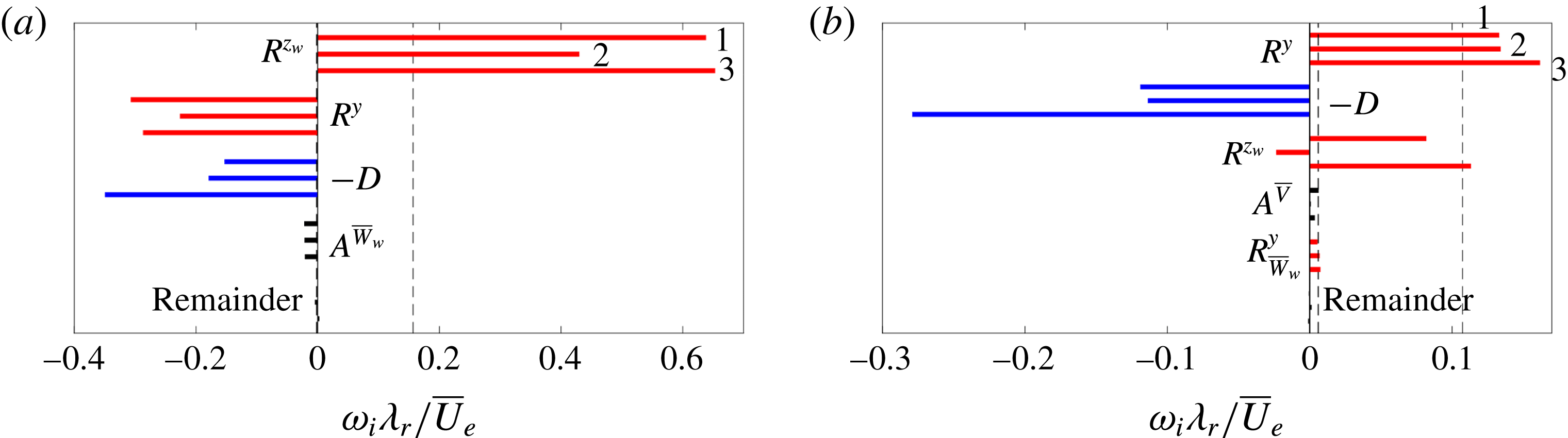
Figure 29.
 $\unicode[STIX]{x1D714}_{i}$
-budgets (bars) of type I (a) and II (b),
$\unicode[STIX]{x1D714}_{i}$
-budgets (bars) of type I (a) and II (b),
 $\unicode[STIX]{x1D714}$
eigenvalues (dashed lines). Bar triplets: strong vortex, nominal
$\unicode[STIX]{x1D714}$
eigenvalues (dashed lines). Bar triplets: strong vortex, nominal
 $Re$
(top, ‘1’); weak vortex, nominal
$Re$
(top, ‘1’); weak vortex, nominal
 $Re$
(middle, ‘2’); strong vortex, lower Reynolds number (bottom, ‘3’):
$Re$
(middle, ‘2’); strong vortex, lower Reynolds number (bottom, ‘3’):
 $10^{-0.54}Re$
(a) and
$10^{-0.54}Re$
(a) and
 $10^{-0.55}Re$
(b).
$10^{-0.55}Re$
(b).
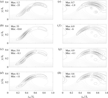
Figure 30. Imaginary part of the (a,e)
 $R^{y}$
-, (b,f)
$R^{y}$
-, (b,f)
 $R^{z_{w}}$
-, (c,g)
$R^{z_{w}}$
-, (c,g)
 $A^{\overline{V}}$
- and (d,h)
$A^{\overline{V}}$
- and (d,h)
 $A^{\overline{W}_{w}}$
-integrands for type I (a–d) and II (e–h) on the weaker vortex (9 levels span (b)
$A^{\overline{W}_{w}}$
-integrands for type I (a–d) and II (e–h) on the weaker vortex (9 levels span (b)
 $[-0.300,47.2]$
, (c)
$[-0.300,47.2]$
, (c)
 $[-0.873,7.62]$
, (d)
$[-0.873,7.62]$
, (d)
 $[-4.69,5.59]$
, (e)
$[-4.69,5.59]$
, (e)
 $[-6.74,4.42]$
, (f)
$[-6.74,4.42]$
, (f)
 $[-8.76,6.21]$
, (g)
$[-8.76,6.21]$
, (g)
 $[-3.20,4.00]$
, (h)
$[-3.20,4.00]$
, (h)
 $[-5.01,3.56]$
, negative contours are dashed). Levels in (a) span
$[-5.01,3.56]$
, negative contours are dashed). Levels in (a) span
 $[-27.8,-3.63]$
with
$[-27.8,-3.63]$
with
 $\unicode[STIX]{x1D6E5}=4.84$
, and
$\unicode[STIX]{x1D6E5}=4.84$
, and
 $[0.300,0.900]$
,
$[0.300,0.900]$
,
 $\unicode[STIX]{x1D6E5}=0.300$
. All values are given in
$\unicode[STIX]{x1D6E5}=0.300$
. All values are given in
 $\overline{U}_{e}/\unicode[STIX]{x1D706}_{r}^{3}$
-units. Eigenfunction contour
$\overline{U}_{e}/\unicode[STIX]{x1D706}_{r}^{3}$
-units. Eigenfunction contour
 $|\tilde{u} _{w}|/\max |\tilde{u} _{w}|=1/6$
(dash-dotted lines).
$|\tilde{u} _{w}|/\max |\tilde{u} _{w}|=1/6$
(dash-dotted lines).
 $\overline{U}_{w}/\overline{U}_{e}$
levels
$\overline{U}_{w}/\overline{U}_{e}$
levels
 $0.1,0.2,\ldots ,0.9$
(dotted) for the weak vortex.
$0.1,0.2,\ldots ,0.9$
(dotted) for the weak vortex.
The previous analysis clarifies that while the spatial topology of the type I and type II modes is rather insensitive to mild changes in the base flow, their respective growth rates are strongly affected. To identify the physical mechanism that renders the eigenmodes more stable for the weaker vortex, the energy balances corresponding to the most unstable modes is displayed in figure 29 (top and middle bars per term). For the type I mode, the vortex strength difference leads to a decrease of both
 $R^{y}$
and
$R^{y}$
and
 $R^{z_{w}}$
in the
$R^{z_{w}}$
in the
 $\unicode[STIX]{x1D714}_{i}$
-budget. Note that the size of
$\unicode[STIX]{x1D714}_{i}$
-budget. Note that the size of
 $A^{\overline{W}_{w}}$
persists. The topology of the production terms related to the Reynolds stress and advection terms is represented in figure 30. The highest level contours are nearly identical to those observed in figures 12 and 13, which explains the similarity of the
$A^{\overline{W}_{w}}$
persists. The topology of the production terms related to the Reynolds stress and advection terms is represented in figure 30. The highest level contours are nearly identical to those observed in figures 12 and 13, which explains the similarity of the
 $\unicode[STIX]{x1D714}_{i}$
-budgets. The shape displayed by the lower contour levels is quite different, however, and explains the differences in the eigenfunction shape. As the
$\unicode[STIX]{x1D714}_{i}$
-budgets. The shape displayed by the lower contour levels is quite different, however, and explains the differences in the eigenfunction shape. As the
 $\unicode[STIX]{x2202}\overline{U}_{w}/\unicode[STIX]{x2202}z_{w}$
shear component is smaller for the weaker vortex, other productive contributions come into play in the region located above the primary vortex. Figure 30(a,c,d) shows productive contributions by the integrands of
$\unicode[STIX]{x2202}\overline{U}_{w}/\unicode[STIX]{x2202}z_{w}$
shear component is smaller for the weaker vortex, other productive contributions come into play in the region located above the primary vortex. Figure 30(a,c,d) shows productive contributions by the integrands of
 $R^{y}$
,
$R^{y}$
,
 $A^{\overline{V}}$
and
$A^{\overline{V}}$
and
 $A^{\overline{W}_{w}}$
, respectively. The downwards protrusion of the eigenfunction about the point
$A^{\overline{W}_{w}}$
, respectively. The downwards protrusion of the eigenfunction about the point
 $(z_{w},y)/\unicode[STIX]{x1D706}_{r}=(0.45;0.22)$
in figure 10(a), associated with the marginally positive
$(z_{w},y)/\unicode[STIX]{x1D706}_{r}=(0.45;0.22)$
in figure 10(a), associated with the marginally positive
 $R^{y}$
contribution in figure 12(a), is absent in figure 28(a). In figure 30(a), the equivalent
$R^{y}$
contribution in figure 12(a), is absent in figure 28(a). In figure 30(a), the equivalent
 $R^{y}$
-integrand contours have a smaller magnitude and extend less in the direction orthogonal to the shear layer. The local maximum of the
$R^{y}$
-integrand contours have a smaller magnitude and extend less in the direction orthogonal to the shear layer. The local maximum of the
 $R^{y}$
-integrand in the neighbourhood of the protrusion has dropped from 1.41 to
$R^{y}$
-integrand in the neighbourhood of the protrusion has dropped from 1.41 to
 $0.92\,\overline{U}_{e}/\unicode[STIX]{x1D706}_{r}^{3}$
for the strong and weak vortices, respectively.
$0.92\,\overline{U}_{e}/\unicode[STIX]{x1D706}_{r}^{3}$
for the strong and weak vortices, respectively.
For the type II mode, unexpectedly, the main Reynolds stress production term,
 $R^{y}$
, exerts a virtually identical contribution in the
$R^{y}$
, exerts a virtually identical contribution in the
 $\unicode[STIX]{x1D714}_{i}$
-budget shown in figure 29. In fact, the production term
$\unicode[STIX]{x1D714}_{i}$
-budget shown in figure 29. In fact, the production term
 $R^{z_{w}}$
is largely responsible for the stabilization relative to the stronger vortex. This illustrates that, although the type II instability is mainly generated by the Reynolds stress associated with the
$R^{z_{w}}$
is largely responsible for the stabilization relative to the stronger vortex. This illustrates that, although the type II instability is mainly generated by the Reynolds stress associated with the
 $\unicode[STIX]{x2202}\overline{U}_{w}/\unicode[STIX]{x2202}y$
shear component, in this case the other component is the main translator of the vortex strength. The apparent link between the spanwise location of the eigenfunction’s maximum and the Reynolds stress
$\unicode[STIX]{x2202}\overline{U}_{w}/\unicode[STIX]{x2202}y$
shear component, in this case the other component is the main translator of the vortex strength. The apparent link between the spanwise location of the eigenfunction’s maximum and the Reynolds stress
 $R^{z_{w}}$
, first encountered in § 4.2, reappears here; as the maximum of the eigenfunction moves in the positive
$R^{z_{w}}$
, first encountered in § 4.2, reappears here; as the maximum of the eigenfunction moves in the positive
 $z_{w}$
-direction, this production term decreases. The relation to the topology of the production term can be deduced by comparing figure 30(f) with 12(d). The negative contours have approximately the same magnitude, but the positive productive contours change quite considerably, the maximum reducing from 16.2 to
$z_{w}$
-direction, this production term decreases. The relation to the topology of the production term can be deduced by comparing figure 30(f) with 12(d). The negative contours have approximately the same magnitude, but the positive productive contours change quite considerably, the maximum reducing from 16.2 to
 $6.9\,\overline{U}_{e}/\unicode[STIX]{x1D706}_{r}^{3}$
for the strong and weak vortices, respectively. Lastly, although it has a small overall magnitude,
$6.9\,\overline{U}_{e}/\unicode[STIX]{x1D706}_{r}^{3}$
for the strong and weak vortices, respectively. Lastly, although it has a small overall magnitude,
 $A^{\overline{V}}$
reduces significantly in the
$A^{\overline{V}}$
reduces significantly in the
 $\unicode[STIX]{x1D714}_{i}$
-budget; it is comparable to the decrease in
$\unicode[STIX]{x1D714}_{i}$
-budget; it is comparable to the decrease in
 $D$
. Comparing figures 30(g) and 13(d), the levels corresponding to the weaker vortex are smaller and are more balanced in the
$D$
. Comparing figures 30(g) and 13(d), the levels corresponding to the weaker vortex are smaller and are more balanced in the
 $z_{w}$
-direction than those corresponding to the stronger vortex.
$z_{w}$
-direction than those corresponding to the stronger vortex.
4.8 Effect of periodic boundary conditions
As mentioned in § 3, the measured flow fields of the single strong and weak vortices have not been periodized. The coefficients are left discontinuous across the boundary, such that no artificial shear layer is introduced. To assess the impact of this approach on the solutions, the problem was set up for the domain containing both vortices, as shown in figure 3, herein denoted as the double-vortex domain. The problem was evaluated at the most unstable wavenumbers presented in table 3. Given the domain is twice as large, the resolution had to be increased accordingly. The currently available resources maximally allowed
 $N_{z}\times N_{y}=140\times 70$
, which, for this domain, represents a resolution in between the cases
$N_{z}\times N_{y}=140\times 70$
, which, for this domain, represents a resolution in between the cases
 $55\times 55$
and
$55\times 55$
and
 $90\times 90$
on the single-vortex domains.
$90\times 90$
on the single-vortex domains.

Figure 31.
 $|\tilde{u} _{w}|/\max |\tilde{u} _{w}|$
for type I (a) and II (b) (levels span [
$|\tilde{u} _{w}|/\max |\tilde{u} _{w}|$
for type I (a) and II (b) (levels span [
 $1/6~5/6$
] with
$1/6~5/6$
] with
 $\unicode[STIX]{x1D6E5}=1/6$
) of respective modes for both vortices, computed on the single (filled contours) and double (dashed) domain. To emphasize: the eigenfunctions on the different vortices correspond to different eigenvalues; each has a support limited to one vortex.
$\unicode[STIX]{x1D6E5}=1/6$
) of respective modes for both vortices, computed on the single (filled contours) and double (dashed) domain. To emphasize: the eigenfunctions on the different vortices correspond to different eigenvalues; each has a support limited to one vortex.
 $\overline{U}_{w}/\overline{U}_{e}$
levels
$\overline{U}_{w}/\overline{U}_{e}$
levels
 $0.1,0.2,\ldots ,0.9$
(dotted). Domain separation for strong (right) and weak (left) vortex (vertical dotted line,
$0.1,0.2,\ldots ,0.9$
(dotted). Domain separation for strong (right) and weak (left) vortex (vertical dotted line,
 $z_{w}/\unicode[STIX]{x1D706}_{r}=0$
).
$z_{w}/\unicode[STIX]{x1D706}_{r}=0$
).
The resulting eigenvalues match up to
 $O(10^{-4})$
absolute errors with those presented in table 3, and effectively collapse in figure 27. The corresponding eigenfunctions are shown in figure 31. Note that each eigenfunction on the different vortices corresponds to a different eigenvalue in the spectrum of the double-vortex domain problem. They are compared to the eigenfunctions retrieved with the single-vortex domains, adjusted to appropriately illustrate their support on the double-vortex domain, using the periodic boundary conditions. All eigenfunctions match perfectly, even the smaller amplitude contours of the type II mode on the weak (left) vortex. Moreover, despite the fact this eigenfunction significantly protrudes the
$O(10^{-4})$
absolute errors with those presented in table 3, and effectively collapse in figure 27. The corresponding eigenfunctions are shown in figure 31. Note that each eigenfunction on the different vortices corresponds to a different eigenvalue in the spectrum of the double-vortex domain problem. They are compared to the eigenfunctions retrieved with the single-vortex domains, adjusted to appropriately illustrate their support on the double-vortex domain, using the periodic boundary conditions. All eigenfunctions match perfectly, even the smaller amplitude contours of the type II mode on the weak (left) vortex. Moreover, despite the fact this eigenfunction significantly protrudes the
 $z_{w}/\unicode[STIX]{x1D706}_{r}=0$
boundary, it does not experience distortion due to the minor discontinuity in the coefficients for the single-vortex domain. This illustrates that, in this case, using discontinuous coefficients across the boundary is justified.
$z_{w}/\unicode[STIX]{x1D706}_{r}=0$
boundary, it does not experience distortion due to the minor discontinuity in the coefficients for the single-vortex domain. This illustrates that, in this case, using discontinuous coefficients across the boundary is justified.
These results are very similar to those presented by Bonfigli & Kloker (Reference Bonfigli and Kloker2007, cf. § 6.2) and Choudhari et al. (Reference Choudhari, Li and Paredes2016). The current results corroborate the notion that the type I and II eigenmodes on different vortices do not participate in the same resonance; they correspond to different modes in the collective spectrum. In this sense, they are proper discrete modes. In addition, in this case, the single-vortex domain problems are representative of the dynamics in the double-vortex domain. So, it is deduced that, given the primary vortices are reasonably separated in space, it is not necessary to consider the more expensive double-vortex domain problem. Neighbouring primary vortices do not contribute crucial information, in that case.
4.9 Reynolds number dependence
Following the analysis of Bonfigli & Kloker (Reference Bonfigli and Kloker2007), the type I and II modes are Kelvin–Helmholtz instabilities and hence display an independency of the Reynolds number when large enough; this is as opposed to viscous Tollmien–Schlichting instabilities that are stable in the Rayleigh limit, see Schlichting et al. (Reference Schlichting, Krause, Oertel, Gersten and Mayes2003) and Drazin & Reid (Reference Drazin and Reid2004). The stability problem for the strong vortex is solved, varying the Reynolds number artificially and fixing all other parameters. The type I and II modes are each evaluated at the most unstable wavenumber (
 $\unicode[STIX]{x1D6FC}\unicode[STIX]{x1D706}_{r}=6.2$
and 8.6, respectively). With increasing Reynolds number, the eigenfunction shapes become very slender. Therefore a
$\unicode[STIX]{x1D6FC}\unicode[STIX]{x1D706}_{r}=6.2$
and 8.6, respectively). With increasing Reynolds number, the eigenfunction shapes become very slender. Therefore a
 $90\times 90$
grid is used to ensure accurately capturing all structural details.
$90\times 90$
grid is used to ensure accurately capturing all structural details.
It is well known that viscosity has a significant impact on the stability of free shear layers when the parameter
 $$\begin{eqnarray}\displaystyle & \displaystyle \unicode[STIX]{x1D6FC}{\displaystyle \frac{\unicode[STIX]{x1D6FF}_{v}}{2}}\,Re_{\unicode[STIX]{x1D6FF}_{v}}\equiv \unicode[STIX]{x1D6FC}{\displaystyle \frac{\unicode[STIX]{x1D6FF}_{v}}{2}}\,{\displaystyle \frac{\unicode[STIX]{x0394}\overline{U}_{w}\,\unicode[STIX]{x1D6FF}_{v}}{4\unicode[STIX]{x1D708}}}=\unicode[STIX]{x1D6FC}{\displaystyle \frac{\unicode[STIX]{x1D6FF}_{v}}{2}}\,{\displaystyle \frac{\unicode[STIX]{x0394}\overline{U}_{w}/2}{\overline{U}_{e}}}{\displaystyle \frac{\unicode[STIX]{x1D6FF}_{v}/2}{\unicode[STIX]{x1D706}_{r}}}Re, & \displaystyle\end{eqnarray}$$
is of
 $o(10^{2})$
(small-
$o(10^{2})$
(small-
 $o$
notation) (Tatsumi, Gotoh & Ayukawa Reference Tatsumi, Gotoh and Ayukawa1964; Michalke Reference Michalke1972). Here,
$o$
notation) (Tatsumi, Gotoh & Ayukawa Reference Tatsumi, Gotoh and Ayukawa1964; Michalke Reference Michalke1972). Here,
 $\unicode[STIX]{x1D6FF}_{v}$
and
$\unicode[STIX]{x1D6FF}_{v}$
and
 $\unicode[STIX]{x0394}\overline{U}_{w}$
are the vorticity thickness and velocity difference relevant for the particular instability. In the present case, these parameters are determined by quantifying the in-plane shear components
$\unicode[STIX]{x0394}\overline{U}_{w}$
are the vorticity thickness and velocity difference relevant for the particular instability. In the present case, these parameters are determined by quantifying the in-plane shear components
 $\unicode[STIX]{x2202}\overline{U}_{w}/\unicode[STIX]{x2202}z_{w}$
and
$\unicode[STIX]{x2202}\overline{U}_{w}/\unicode[STIX]{x2202}z_{w}$
and
 $\unicode[STIX]{x2202}\overline{U}_{w}/\unicode[STIX]{x2202}y$
at the location where the
$\unicode[STIX]{x2202}\overline{U}_{w}/\unicode[STIX]{x2202}y$
at the location where the
 $|\tilde{u} |$
-amplitude is maximal. Along the direction indicated by the shear components, denoted by
$|\tilde{u} |$
-amplitude is maximal. Along the direction indicated by the shear components, denoted by
 $\unicode[STIX]{x1D703}$
, the closest minimum or, if no minimum exists, the closest ‘favourable’ inflection point of
$\unicode[STIX]{x1D703}$
, the closest minimum or, if no minimum exists, the closest ‘favourable’ inflection point of
 $\overline{U}_{w}$
is determined under the layer of interest. The difference between the free-stream velocity and
$\overline{U}_{w}$
is determined under the layer of interest. The difference between the free-stream velocity and
 $\overline{U}_{w}$
at this point is
$\overline{U}_{w}$
at this point is
 $\unicode[STIX]{x0394}\overline{U}_{w}$
. The vorticity thickness is defined as:
$\unicode[STIX]{x0394}\overline{U}_{w}$
. The vorticity thickness is defined as:
 $$\begin{eqnarray}\displaystyle & \displaystyle \unicode[STIX]{x1D6FF}_{v}\equiv {\displaystyle \frac{\unicode[STIX]{x0394}\overline{U}_{w}}{\sqrt{\left({\displaystyle \frac{\unicode[STIX]{x2202}\overline{U}_{w}}{\unicode[STIX]{x2202}z_{w}}}\right)^{2}+\left({\displaystyle \frac{\unicode[STIX]{x2202}\overline{U}_{w}}{\unicode[STIX]{x2202}y}}\right)^{2}}}}. & \displaystyle\end{eqnarray}$$
The inset in figure 32 illustrates the location at which the shear components are extracted together with the vorticity thickness
 $\unicode[STIX]{x1D6FF}_{v}$
and orientation
$\unicode[STIX]{x1D6FF}_{v}$
and orientation
 $\unicode[STIX]{x1D703}$
. All relevant parameters are reported in table 4, including: the parameter
$\unicode[STIX]{x1D703}$
. All relevant parameters are reported in table 4, including: the parameter
 $\unicode[STIX]{x1D6FC}\unicode[STIX]{x1D6FF}_{v}Re_{\unicode[STIX]{x1D6FF}_{v}}/2$
, the extraction location, the
$\unicode[STIX]{x1D6FC}\unicode[STIX]{x1D6FF}_{v}Re_{\unicode[STIX]{x1D6FF}_{v}}/2$
, the extraction location, the
 $\overline{U}_{w}$
-shear components and the angle
$\overline{U}_{w}$
-shear components and the angle
 $\unicode[STIX]{x1D703}$
. Using these scales, customized for each mode, insight is gained into the relative ‘efficiency’ of the type I with respect to the II mode.
$\unicode[STIX]{x1D703}$
. Using these scales, customized for each mode, insight is gained into the relative ‘efficiency’ of the type I with respect to the II mode.
The growth rates in the
 $\unicode[STIX]{x1D6FF}_{v}$
-scaling are presented with full black symbols in figure 32. It is evident that the growth rates saturate with increasing Reynolds number. Viscosity has a significant effect in the nominal case. This is as expected, because all values
$\unicode[STIX]{x1D6FF}_{v}$
-scaling are presented with full black symbols in figure 32. It is evident that the growth rates saturate with increasing Reynolds number. Viscosity has a significant effect in the nominal case. This is as expected, because all values
 $\unicode[STIX]{x1D6FC}\unicode[STIX]{x1D6FF}_{v}Re_{\unicode[STIX]{x1D6FF}_{v}}/2<100$
. The parameter values for the type II mode are smaller than those for type I, causing the type II growth rate to saturate more slowly.
$\unicode[STIX]{x1D6FC}\unicode[STIX]{x1D6FF}_{v}Re_{\unicode[STIX]{x1D6FF}_{v}}/2<100$
. The parameter values for the type II mode are smaller than those for type I, causing the type II growth rate to saturate more slowly.
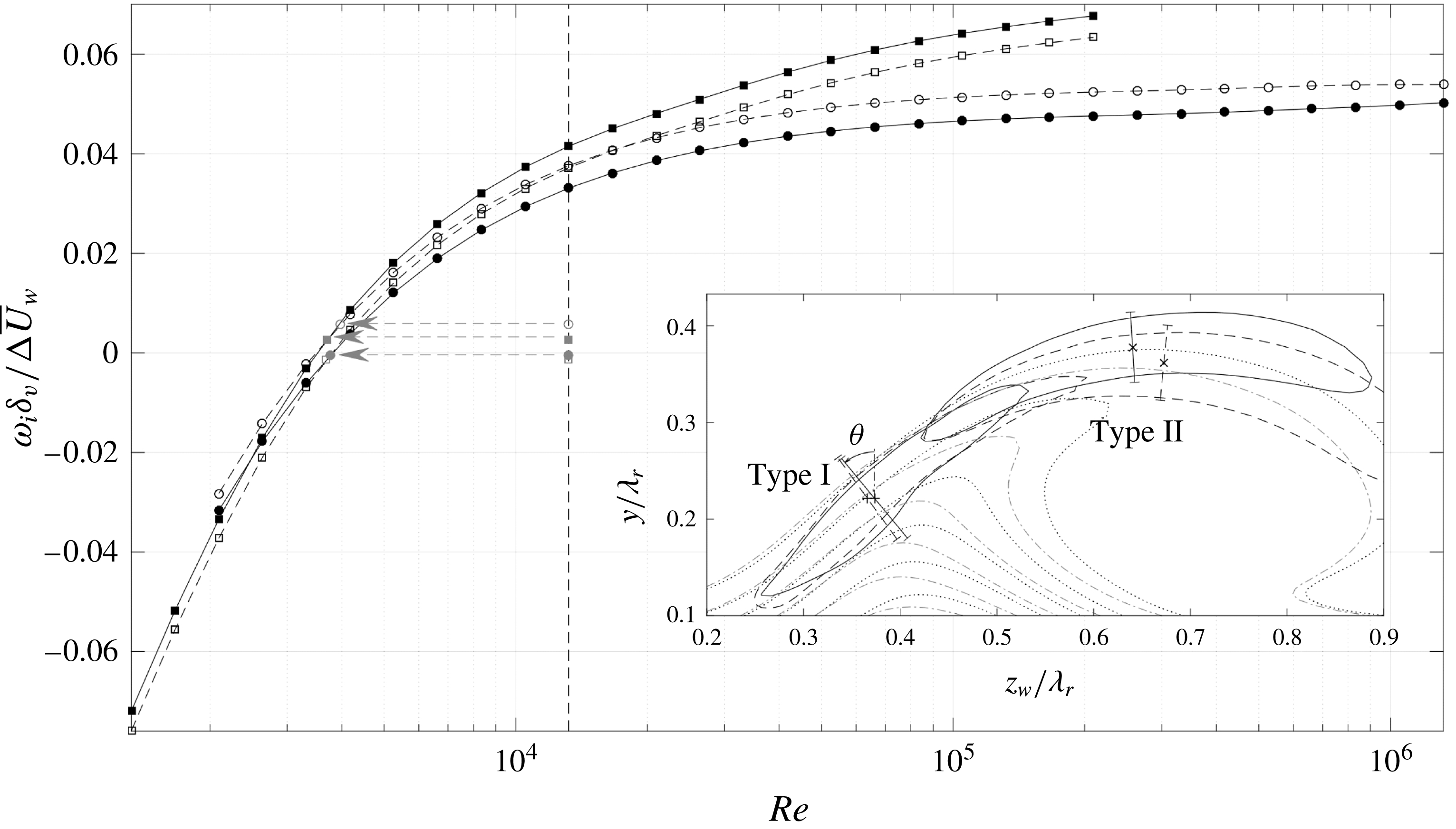
Figure 32. Type I (
 $\unicode[STIX]{x1D6FC}\unicode[STIX]{x1D706}_{r}=6.2$
, circles) and II (
$\unicode[STIX]{x1D6FC}\unicode[STIX]{x1D706}_{r}=6.2$
, circles) and II (
 $8.6$
, squares) growth rate in
$8.6$
, squares) growth rate in
 $\unicode[STIX]{x1D6FF}_{v}$
-scaling versus
$\unicode[STIX]{x1D6FF}_{v}$
-scaling versus
 $Re$
for the strong vortex. Eigenvalues: computed (filled symbols), excluding
$Re$
for the strong vortex. Eigenvalues: computed (filled symbols), excluding
 $A^{\overline{V}}$
and
$A^{\overline{V}}$
and
 $A^{\overline{W}_{w}}$
(open symbols), weak vortex (grey symbols). Nominal
$A^{\overline{W}_{w}}$
(open symbols), weak vortex (grey symbols). Nominal
 $Re$
(vertical dashed line), interpolation of weak vortex onto strong vortex data (arrows). Inset:
$Re$
(vertical dashed line), interpolation of weak vortex onto strong vortex data (arrows). Inset:
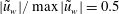 $|\tilde{u} _{w}|/\max |\tilde{u} _{w}|=0.5$
for both modes at nominal
$|\tilde{u} _{w}|/\max |\tilde{u} _{w}|=0.5$
for both modes at nominal
 $Re$
and
$Re$
and
 $\overline{U}_{w}/\overline{U}_{e}$
levels
$\overline{U}_{w}/\overline{U}_{e}$
levels
 $0.4,0.5,\ldots ,0.9$
for the strong (solid respectively dotted lines) and weak (dashed respectively dash-dotted) vortex.
$0.4,0.5,\ldots ,0.9$
for the strong (solid respectively dotted lines) and weak (dashed respectively dash-dotted) vortex.
 $|\tilde{u} |$
-maximum location (crosses) and
$|\tilde{u} |$
-maximum location (crosses) and
 $\unicode[STIX]{x1D6FF}_{v}$
in the
$\unicode[STIX]{x1D6FF}_{v}$
in the
 $\unicode[STIX]{x1D703}$
-direction (bars).
$\unicode[STIX]{x1D703}$
-direction (bars).
It is striking that the type II mode is the most unstable of the two, in the custom per-mode scaling. The type II mode is the more efficient mechanism. This suggests that the Reynolds stress production terms do not contribute to the growth rate as in the case of a one-dimensional shear layer. For the strong vortex, both shear components act constructively for the type II mode, while the
 $\unicode[STIX]{x2202}\overline{U}_{w}/\unicode[STIX]{x2202}y$
component acts destructively for the type I mode. However, next to these Reynolds stresses, there are effects associated with the in-plane velocity components; i.e. the equivalents of non-parallel flow effects. The largest contributions in the
$\unicode[STIX]{x2202}\overline{U}_{w}/\unicode[STIX]{x2202}y$
component acts destructively for the type I mode. However, next to these Reynolds stresses, there are effects associated with the in-plane velocity components; i.e. the equivalents of non-parallel flow effects. The largest contributions in the
 $\unicode[STIX]{x1D714}_{i}$
-balance, except
$\unicode[STIX]{x1D714}_{i}$
-balance, except
 $D$
, are found to vary mildly with the Reynolds number as shown in figure 29 (compare top and bottom bars per term). Only the Reynolds stress production terms in the type II budget show an increase, but have the same character. The non-parallel contributions also retain the same character;
$D$
, are found to vary mildly with the Reynolds number as shown in figure 29 (compare top and bottom bars per term). Only the Reynolds stress production terms in the type II budget show an increase, but have the same character. The non-parallel contributions also retain the same character;
 $\overline{V}$
-advection destabilizes the type II mode and the
$\overline{V}$
-advection destabilizes the type II mode and the
 $\overline{W}_{w}$
-term stabilizes type I.
$\overline{W}_{w}$
-term stabilizes type I.
Table 4. Vorticity thickness parameters for the nominal most unstable modes. Shear component values are in units of
 $\overline{U}_{e}/\unicode[STIX]{x1D706}_{r}$
.
$\overline{U}_{e}/\unicode[STIX]{x1D706}_{r}$
.
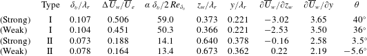
Based on the previous observations, further links are sought between growth, base flow strength and Reynolds number. Figure 32 suggests the eigensolutions corresponding to the weak vortex have common features with those on the strong vortex at a lower Reynolds number. The horizontal arrows in figure 32 indicate the interpolation of the weak vortex growth rates onto the curve with varying Reynolds number of the strong vortex. This interpolation yields nearly matching Reynolds numbers for both mode types,
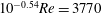 $10^{-0.54}Re=3770$
for type I and
$10^{-0.54}Re=3770$
for type I and
 $10^{-0.55}Re=3700$
for type II. The mild variation in the energy budgets with the Reynolds number mentioned before implies that the increased viscous dissipation term is directly equivalent to the net reduction of the Reynolds stress terms for the weaker vortex case. Figure 29 visualizes this; the energy budgets are given for these specific Reynolds numbers. For the type II instability, for example, the change in
$10^{-0.55}Re=3700$
for type II. The mild variation in the energy budgets with the Reynolds number mentioned before implies that the increased viscous dissipation term is directly equivalent to the net reduction of the Reynolds stress terms for the weaker vortex case. Figure 29 visualizes this; the energy budgets are given for these specific Reynolds numbers. For the type II instability, for example, the change in
 $D$
closely matches the change in the
$D$
closely matches the change in the
 $R^{z_{w}}$
-term.
$R^{z_{w}}$
-term.
Despite these equivalences, the eigenfunctions for the two cases are different. As mentioned before, the main dependency of the eigenfunctions on the Reynolds number is their respective width orthogonal to the shear layer. The eigenfunctions corresponding to the strong vortex are shown in figure 33 for various Reynolds numbers. For an increasing Reynolds number, the eigenfunction focuses about the region where the Reynolds stresses are active. The increase in width is caused by viscous diffusion. The distinction is attributed to the fact that the dissipation acts on all velocity components, while both dominant Reynolds stress terms produce or destroy the
 $\tilde{u} _{w}$
component directly. In the weak vortex case the latter is reduced causing a redistribution of the energy balance at local points in the
$\tilde{u} _{w}$
component directly. In the weak vortex case the latter is reduced causing a redistribution of the energy balance at local points in the
 $z_{w}y$
-plane. The decreased Reynolds number instead has a global impact on all terms, which does not cause a significant redistribution within the plane.
$z_{w}y$
-plane. The decreased Reynolds number instead has a global impact on all terms, which does not cause a significant redistribution within the plane.
Using the energy decomposition, the solely parallel effects can be separated from the total contributions in the eigenvalue information. This is done by subtracting all contributions involving the
 $\overline{V}$
- and
$\overline{V}$
- and
 $\overline{W}_{w}$
-components from the computed eigenvalue, i.e. all associated advection and Reynolds stress terms, including those in the remainder. The results are the empty symbols shown in figure 32. It is revealed that, in close proximity to the nominal Reynolds number for the strong vortex case, the modes are equally matched. In terms of the growth rate, this demonstrates both mode types are the offspring of the same parallel instability mechanism. This is a non-trivial result regarding the productive and destructive character of the Reynolds stress terms. Nevertheless, the cumulative effect is the same in this particular range.
$\overline{W}_{w}$
-components from the computed eigenvalue, i.e. all associated advection and Reynolds stress terms, including those in the remainder. The results are the empty symbols shown in figure 32. It is revealed that, in close proximity to the nominal Reynolds number for the strong vortex case, the modes are equally matched. In terms of the growth rate, this demonstrates both mode types are the offspring of the same parallel instability mechanism. This is a non-trivial result regarding the productive and destructive character of the Reynolds stress terms. Nevertheless, the cumulative effect is the same in this particular range.
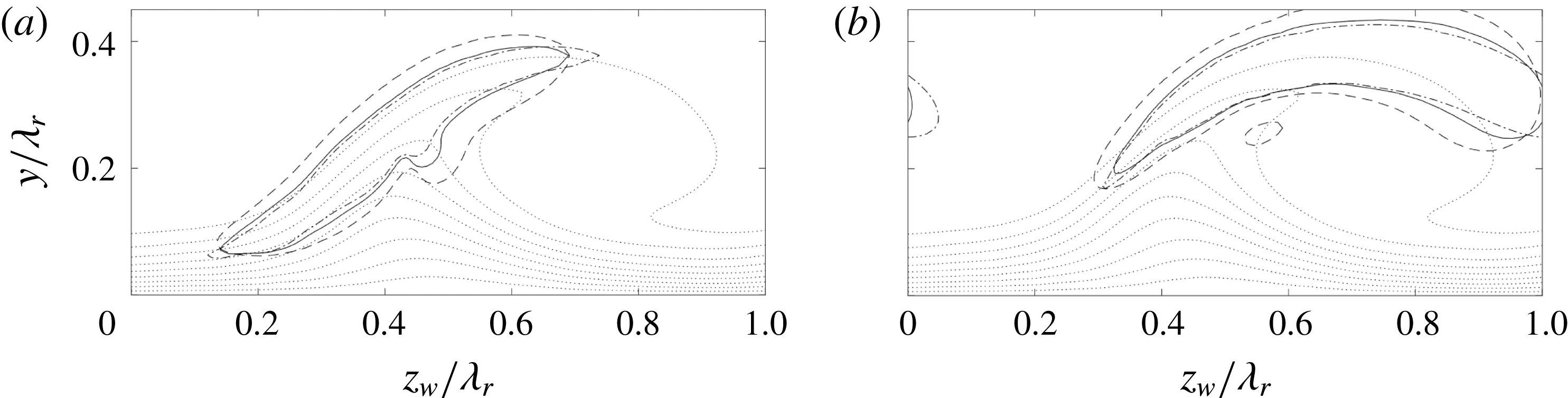
Figure 33.
 $|\tilde{u} _{w}|/\max |\tilde{u} _{w}|=1/6$
for Reynolds number:
$|\tilde{u} _{w}|/\max |\tilde{u} _{w}|=1/6$
for Reynolds number:
 $10^{-0.8}Re$
(dashed line), nominal (solid) and
$10^{-0.8}Re$
(dashed line), nominal (solid) and
 $10^{0.8}Re$
(dash-dotted) for type I (a) and II (b).
$10^{0.8}Re$
(dash-dotted) for type I (a) and II (b).
 $\overline{U}_{w}/\overline{U}_{e}$
levels
$\overline{U}_{w}/\overline{U}_{e}$
levels
 $0.1,0.2,\ldots ,0.9$
(dotted).
$0.1,0.2,\ldots ,0.9$
(dotted).
The previous analysis demonstrates that the eigensolutions incorporating all non-parallel effects, including non-trivial redistribution, generation and destruction effects imposed by the
 $\overline{V}$
- and
$\overline{V}$
- and
 $\overline{W}_{w}$
-components, can be recast into a self-similar parallel form that only depends on the details associated with the main shear layers, viz.
$\overline{W}_{w}$
-components, can be recast into a self-similar parallel form that only depends on the details associated with the main shear layers, viz.
 $\unicode[STIX]{x1D6FF}_{v}$
and
$\unicode[STIX]{x1D6FF}_{v}$
and
 $\unicode[STIX]{x0394}\overline{U}_{w}$
. Capturing those details sets the main physical basis of the perturbation and the non-parallel velocity components are extra effects. Note that the reverse approach, i.e. performing the stability analysis on the
$\unicode[STIX]{x0394}\overline{U}_{w}$
. Capturing those details sets the main physical basis of the perturbation and the non-parallel velocity components are extra effects. Note that the reverse approach, i.e. performing the stability analysis on the
 $\overline{U}_{w}$
-field only, does not necessarily yield the same result due to the redistribution imposed by the in-plane velocity components.
$\overline{U}_{w}$
-field only, does not necessarily yield the same result due to the redistribution imposed by the in-plane velocity components.
From the relationship governing the inviscid stability of the piecewise linear shear layer, see Drazin & Reid (Reference Drazin and Reid2004):
 $$\begin{eqnarray}\displaystyle & \displaystyle (2\unicode[STIX]{x1D714}\unicode[STIX]{x1D6FF}_{v}/\unicode[STIX]{x0394}\overline{U}_{w})^{2}=(1-2\unicode[STIX]{x1D6FC}\unicode[STIX]{x1D6FF}_{v})^{2}-(\text{e}^{-2\unicode[STIX]{x1D6FC}\unicode[STIX]{x1D6FF}_{v}})^{2}, & \displaystyle\end{eqnarray}$$
the maximal temporal growth rate
 $\unicode[STIX]{x1D714}_{i}=0.2012\unicode[STIX]{x0394}\overline{U}_{w}/\unicode[STIX]{x1D6FF}_{v}$
is found, which is significantly larger than the limiting values shown in figure 32. Although it is not in the scope of the current paper, next to the destructive nature of the Reynolds stress terms, other effects like the two-dimensionality imposed by the shear layer’s finite spanwise extent and wall proximity have to be carefully factored before the results can be expected to be comparable to the one-dimensional shear layer characteristics, see Groot et al. (Reference Groot, Ye, van Oudheusden, Zhang and Pinna2016) (cf. figure 6 (left)). Both effects are stabilizing and not accounted for in the simple scaling. Drazin & Reid (Reference Drazin and Reid2004) show this for the wall proximity. Measured orthogonally with respect to the shear layers, their centres are located more than
$\unicode[STIX]{x1D714}_{i}=0.2012\unicode[STIX]{x0394}\overline{U}_{w}/\unicode[STIX]{x1D6FF}_{v}$
is found, which is significantly larger than the limiting values shown in figure 32. Although it is not in the scope of the current paper, next to the destructive nature of the Reynolds stress terms, other effects like the two-dimensionality imposed by the shear layer’s finite spanwise extent and wall proximity have to be carefully factored before the results can be expected to be comparable to the one-dimensional shear layer characteristics, see Groot et al. (Reference Groot, Ye, van Oudheusden, Zhang and Pinna2016) (cf. figure 6 (left)). Both effects are stabilizing and not accounted for in the simple scaling. Drazin & Reid (Reference Drazin and Reid2004) show this for the wall proximity. Measured orthogonally with respect to the shear layers, their centres are located more than
 $2\unicode[STIX]{x1D6FF}_{v}$
from the wall, which indicates no significant effect. The modes have a wavelength in the
$2\unicode[STIX]{x1D6FF}_{v}$
from the wall, which indicates no significant effect. The modes have a wavelength in the
 $z_{w}y$
-plane parallel to the shear layer, which has a stabilizing effect through viscous dissipation, but is not accounted for in the one-dimensional case. In the case of the strong vortex, the most unstable modes have approximately equal such wavelengths (
$z_{w}y$
-plane parallel to the shear layer, which has a stabilizing effect through viscous dissipation, but is not accounted for in the one-dimensional case. In the case of the strong vortex, the most unstable modes have approximately equal such wavelengths (
 ${\approx}0.3\unicode[STIX]{x1D706}_{r}$
) for the larger part of the domain and therefore has an equal impact for both modes.
${\approx}0.3\unicode[STIX]{x1D706}_{r}$
) for the larger part of the domain and therefore has an equal impact for both modes.
5 Conclusion
A combined experimental and numerical approach to the analysis of the secondary stability of realistic swept-wing boundary layers is presented, as a continuation of the work of Serpieri & Kotsonis (Reference Serpieri and Kotsonis2016). The studied boundary layer develops on the pressure side of a
 $45^{\circ }$
swept wing at an angle of attack (
$45^{\circ }$
swept wing at an angle of attack (
 $Re_{c_{X}}=2.17\times 10^{6}$
,
$Re_{c_{X}}=2.17\times 10^{6}$
,
 $M=0.075$
).
$M=0.075$
).
Bonfigli & Kloker (Reference Bonfigli and Kloker2007) point out that the a complete description of the distorted base flow field is essential when performing the secondary stability analysis, especially regarding the wall-normal and spanwise (in-plane) velocity components. However, how the latter components affect the secondary stability is described only in a conceptual manner. Serpieri & Kotsonis (Reference Serpieri and Kotsonis2016) used tomographic particle image velocimetry (tomo-PIV) that provides such a complete description of the base flow and fluctuations, allowing applying two-dimensional linear stability theory to the measured mean flow.
Two neighbouring primary vortices, of different strength, extracted at the same streamwise location, are considered in the global stability analysis. The two eigenmodes of type I and II (Koch et al. (Reference Koch, Bertolotti, Stolte and Hein2000)), referred to as the
 $z$
- and
$z$
- and
 $y$
-modes of Malik et al. (Reference Malik, Li, Choudhari and Chang1999), are extracted primarily. The type III mode is obtained as well, but it is expected a priori to be affected by the uncertainty of the current PIV measurement near the wall. The attention is therefore focussed on type I and II.
$y$
-modes of Malik et al. (Reference Malik, Li, Choudhari and Chang1999), are extracted primarily. The type III mode is obtained as well, but it is expected a priori to be affected by the uncertainty of the current PIV measurement near the wall. The attention is therefore focussed on type I and II.
The energy decompositions of the type I and II modes are investigated in detail, divulging the contribution of the in-plane velocity components. For the type I mode, the effect is stabilizing and mainly caused by the spanwise velocity component. This imposes a net perturbation energy advection towards the vortex core, decreasing the growth rate by 14.1 %. For mode II, the growth rate is increased by 7 % by advection caused by the wall-normal velocity, that yields a net advection away from the vortex core. Another important difference between the modes regarding advection is that the type I perturbation energy is driven or ‘squeezed’ onto a line, while no such line exists for the type II mode. This renders the position of the type I mode with respect to the primary crossflow vortex more robust than that of the type II mode.
The measured mean flow is subject to an uncertainty, which is highly related to the most energetic POD mode that manifests itself as a spanwise shift of the entire primary vortex structure. A Monte Carlo approach is deployed to investigate the convergence of the results with the number of instantaneous snapshots,
 $N_{fr}$
, used for the mean flow. The mean growth rate and energy decomposition values converge for increasing
$N_{fr}$
, used for the mean flow. The mean growth rate and energy decomposition values converge for increasing
 $N_{fr}$
. The growth rate fluctuations are large, but display a linear convergence trend. Therefore they can be neglected beyond the
$N_{fr}$
. The growth rate fluctuations are large, but display a linear convergence trend. Therefore they can be neglected beyond the
 $N_{fr}$
value where the fluctuations are so small they do not change the solution structure any more. For the type I mode this is straightforward as the arrangement of the energy decomposition is fixed for every considered
$N_{fr}$
value where the fluctuations are so small they do not change the solution structure any more. For the type I mode this is straightforward as the arrangement of the energy decomposition is fixed for every considered
 $N_{fr}$
. For the type II mode, the Reynolds stress production term associated with the spanwise shear component experiences large fluctuations about its mean value. These fluctuations correlate strongly to the movement of the type II eigenfunction in the spanwise direction, which, in turn, is deduced to be the logical result of the most energetic POD mode. The link between the movement and the Reynolds stress production term is physically supported by the topology of the latter. Additionally, the relative sensitivity of the different modes is explained by the different topologies of the in-plane advection terms for the different modes; being more robust for the type I mode.
$N_{fr}$
. For the type II mode, the Reynolds stress production term associated with the spanwise shear component experiences large fluctuations about its mean value. These fluctuations correlate strongly to the movement of the type II eigenfunction in the spanwise direction, which, in turn, is deduced to be the logical result of the most energetic POD mode. The link between the movement and the Reynolds stress production term is physically supported by the topology of the latter. Additionally, the relative sensitivity of the different modes is explained by the different topologies of the in-plane advection terms for the different modes; being more robust for the type I mode.
Using a measured base flow implies the in-plane flow is not divergence free and the fields have to be extrapolated in the wall-normal direction. A crude estimation points out the non-zero divergence yields smaller growth rate changes compared to the observed uncertainty due to the mean ensemble size. The effect of extrapolation is negligible up to the discretization error when using parameters representative of the non-intrusive limit.
The applicability of the Gaster transformation when applied the measured base flow is verified. Despite slight changes in the Reynolds–Orr terms, the spatial and temporal eigenfunctions were found to change negligibly.
The flow structure of the type I eigenmode is compared against that of the POD mode, a main difference being the inclination of the vortex structures. The eigenmode growth is found to be underestimated when compared to a measure based on the POD mode. A cause for this could be the latter’s low phase resolution, when considering only 2 POD modes. Using bandpass filtered hot-wire anemometry results, corresponding to the type I mode, a match is established with the eigenmode growth. This illustrates the approach is capable of extracting the order of magnitude of the growth rates.
Analysing the weak primary vortex, both modes are found to be (marginally) stable. This is in line with the experimental observations, but poses a remarkable difference with respect to the strong vortex. Comparing the growth rates reported in the literature illustrates that both vortices linger close to the neutral limit, explaining the (only apparently) large growth rate difference. The robustness of the growth rate is checked by analysing artificially interpolated base flow solutions. For the type I mode, the Reynolds stress terms related to the wall-normal shear layer and the advection terms now have a more pronounced effect and increase the spanwise extent of the eigenfunction, also encountered by Koch et al. (Reference Koch, Bertolotti, Stolte and Hein2000). Interestingly, the stabilization of the type II mode is mainly caused by a strong decrease in the Reynolds stress production term associated with the spanwise shear layer; while the wall-normal shear layer’s contribution remains identical. Furthermore, the eigenfunction displays a significant rightward lean, which can be directly compared to the behaviour observed in the uncertainty quantification. This manifestation demonstrates that behaviour is indeed physical.
Solving the problem with a domain containing both vortices, virtually identical results are retrieved. This indicates that, for the vortices considered, the periodic boundary conditions influence the results negligibly.
The Kelvin–Helmholtz nature of the type I and II modes (Bonfigli & Kloker Reference Bonfigli and Kloker2007) is confirmed by analysing the strong vortex and artificially changing the Reynolds number. This mainly results in eigenfunction width changes as a consequence of viscous diffusion. The growth rate results displayed in personalized vorticity thickness scaling shows that the type II mode is the more efficient mechanism over type I with respect to the active shear strength. Omitting the terms related to in-plane advection eliminates the difference. This illustrates the impact of the in-plane flow directly and demonstrates that the stability solutions can be cast into a parallel basis form to which the in-plane velocity components pose a deviation. The elimination of the efficiency difference is not universal; despite the correction for the in-plane velocity components the characteristics diverge when considering a larger Reynolds number range and the weak vortex case.
These outcomes indicate, at least for this application, that resolving the shear layers allows extracting stability data. Having to scrutinize the delicate primary vortices’ receptivity in a computational approach is thereby circumvented. With the current approach, these essential features are incorporated in the base flow and, by consequence, in the stability analysis. To model this computationally can be very challenging and requires experimental calibration nonetheless.
More physical understanding results in terms of the solutions’ robustness to realistic perturbations of the problem. Therefore, by bringing the stability approach closer to the experiment, making their ever-present relationship more mutual, a better representation and physical understanding can result. This information can be fed back into the design of further experimental campaigns.
The conclusions of this article are expected to be applicable in a broader range of flow topologies and the methodology can extend experimental measurability at other fronts. For example, the perturbation pressure field can be extracted from a PIV base flow.


 Open access