


1. Introduction
The phenomenon of whistling of deep cavities subject to grazing flow has been studied for decades (East Reference East1966; Rockwell & Naudascher Reference Rockwell and Naudascher1978; Elder, Farabee & Demetz Reference Elder, Farabee and Demetz1982; Forestier, Jacquin & Geffroy Reference Forestier, Jacquin and Geffroy2003). It results from a feedback loop between one of the cavity's acoustic eigenmodes and the unsteady vorticity at its opening (e.g. Bourquard, Faure-Beaulieu & Noiray Reference Bourquard, Faure-Beaulieu and Noiray2021; Ho & Kim Reference Ho and Kim2021). This unsteady vorticity is caused by a Kelvin–Helmholtz instability in the shear layer at the opening of the cavity, resulting from the velocity difference between the fast grazing air flow and the air at rest in the cavity. When this feedback loop becomes unstable, it leads to high-amplitude aeroacoustic limit cycles. While the whistling from rectangular cavities has been investigated in numerous studies, the more complex whistling of axisymmetric cavities, which is the topic of the present work, has received less attention. In such configuration, the aeroacoustic feedback loop frequently involves one of the first azimuthal acoustic modes. There are similarities between these azimuthal aeroacoustic modes and thermoacoustic azimuthal modes in annular combustion chambers, which are intensively studied because of the problems they cause in turbomachines for propulsion and power generation applications. In these annular combustor configurations, the rotational symmetry of the chamber gives rise to pairs of degenerate orthogonal azimuthal thermoacoustic modes, sharing the same eigenfrequency. When the symmetry is imperfect, the degenerate mode pairs transform into pairs of modes with slightly different frequencies and growth rates (Noiray, Bothien & Schuermans Reference Noiray, Bothien and Schuermans2011; Bauerheim et al. Reference Bauerheim, Salas, Nicoud and Poinsot2014). As a side note, this type of problem is not limited to thermoacoustic or aeroacoustic systems, but exists in various fields of physics such as light scattering in microspheres (Mazzei et al. Reference Mazzei, Götzinger, de S. Menezes, Zumofen, Benson and Sandoghar2007) or magnetic waves in micrometric ferromagnetic disks (Hoffmann et al. Reference Hoffmann, Woltersdorf, Perzlmaier, Slavin, Tiberkevitch, Bischof, Weiss and Back2007). In the case of thermoacoustic instabilities, the instantaneous state of azimuthal modes can be described with three categories: spinning modes that propagate at the speed of sound along the annular combustor, standing modes that oscillate with a fixed or slowly drifting orientation and mixed modes that are a linear combination of standing and spinning modes. Experimental observations in academic and industrial configurations have shown that the state of the azimuthal thermoacoustic modes usually wanders between mixed modes with dominant spinning component and mixed modes that are closer to standing states (e.g. Noiray & Schuermans Reference Noiray and Schuermans2013; Worth & Dawson Reference Worth and Dawson2013; Indlekofer et al. Reference Indlekofer, Faure-Beaulieu, Dawson and Noiray2022). The statistical preference for certain states and the transitions between them are associated to the intensity of the turbulent combustion noise, to the presence of a azimuthal mean flow, to small asymmetries of the flow or the geometry and to the nonlinear acoustic response of the flames (e.g. Bauerheim, Cazalens & Poinsot Reference Bauerheim, Cazalens and Poinsot2015; Ghirardo, Juniper & Moeck Reference Ghirardo, Juniper and Moeck2016; Rouwenhorst, Hermann & Polifke Reference Rouwenhorst, Hermann and Polifke2017; Aguilar et al. Reference Aguilar, Dawson, Schuller, Durox, Prieur and Candel2021; Faure-Beaulieu et al. Reference Faure-Beaulieu, Indlekofer, Dawson and Noiray2021a). In the case of an aeroacoustic instability, the acoustic source originates from the coherent unsteady vorticity of the flow. We show that the effects of mean azimuthal flow and system's rotational asymmetries can be included into low-order models in a similar way as they are in annular thermoacoustic systems.
Let us now briefly review key contributions of the last decade to the understanding of azimuthal aeroacoustic instabilities in cylindrical cavities. Aly & Ziada (Reference Aly and Ziada2010) studied experimentally the whistling of a shallow axisymmetric cavity and conducted a parametric study on the effects of the cavity's width and depth on the type of mode, the frequency and the amplitude of the oscillations: depending on the cavity's dimensions and the flow velocity, different combinations of shear layer modes and azimuthal acoustic modes lead to whistling. The authors also showed that, even in an apparently axisymmetric configuration, the observed aeroacoustic modes are not purely spinning but rather mixed modes with a constant preferential orientation (Aly & Ziada Reference Aly and Ziada2011). In the same study, they also investigated experimentally the effects of symmetry breaking by adding splitter plates in the cavity. Furthermore Oshkai & Barannyk (Reference Oshkai and Barannyk2013) investigated the whistling of a deep cylindrical cavity and measured the instantaneous velocity fluctuations of the shear layer with standard particle image velocimetry (PIV). They studied the effect of chamfered cavity edges on the aeroacoustic behaviour (Barannyk & Oshkai Reference Barannyk and Oshkai2014) and the unsteady vorticity field (Oshkai & Barannyk Reference Oshkai and Barannyk2014) in order to provide an insight into mechanisms of whistling in these axisymmetric geometries. Nakiboğlu, Manders & Hirschberg (Reference Nakiboğlu, Manders and Hirschberg2012) used Howe's vortex sound theory (Howe Reference Howe2002) and simulations of the incompressible unsteady Reynolds-averaged Navier–Stokes (RANS) equations of a harmonically forced axisymmetric cavity to predict at which forcing frequency the peak whistling is maximal, depending on the mean flow profile in the pipe and the cavity's aspect ratio. Compressible large eddy simulations (LES) by Wang & Liu (Reference Wang and Liu2020) and Abdelmwgoud, Shaaban & Mohany (Reference Abdelmwgoud, Shaaban and Mohany2020) allowed them to identify the structure of the hydrodynamic fluctuations associated to standing and spinning aeroacoustic modes in axisymmetric cavities. The latter study revealed different vorticity patterns associated with standing and spinning modes. Standing modes give rise to periodic vortex crescents disconnected from each others, while spinning modes are characterised by a continuous helical vortex tube spinning along the cylindrical shear layer. Although the initial mean flow is reflectionally symmetric, this helical mode is not. In the aforementioned LES and in the experiments shown in the present study, the hydrodynamic velocity fluctuations of the shear layer are non-negligible compared with the mean axial velocity in the pipe. Therefore, this symmetry breaking of the hydrodynamic fluctuations is likely to have repercussions on the reflectional symmetry of the mean flow itself and to entail a non-zero mean azimuthal velocity field. In the present paper, we show experimental evidence that a strong azimuthal aeroacoustic instability can indeed induce a whirling flow in an axisymmetric cavity, a phenomenon that had not been reported before in the literature.
This paper is the first part of an experimental and theoretical study on azimuthal aeroacoustic instabilities in deep axisymmetric cavities. It stands at the intersection between the literature on deep cavity whistling and the studies about degenerate or close-to-degenerate azimuthal mode pairs in axisymmetric configurations, revealing and explaining the interplay between the azimuthal acoustic modes, the hydrodynamic helical modes and the mean swirl. Experiments were conducted with a cavity that is the axisymmetric counterpart of the rectangular side cavity studied theoretically, numerically and experimentally by Boujo, Bauerheim & Noiray (Reference Boujo, Bauerheim and Noiray2018), Bourquard et al. (Reference Bourquard, Faure-Beaulieu and Noiray2021) and Pedergnana et al. (Reference Pedergnana, Bourquard, Faure-Beaulieu and Noiray2021). This paper, Part 1, focuses on the hydrodynamic aspects of the aeroacoustic feedback in absence of mean swirl upstream of the cavity, and on the effect of the aeroacoustic oscillations on the onset of a mean swirl in the cavity. Reference Faure-Beaulieu, Pedergnana and NoirayPart 2 deals with the complementary problem of the effect of a mean swirl imposed upstream of the cavity onto the modal dynamics of the aeroacoustic instability. In § 2, the set-up is presented and the results of acoustic and stereoscopic PIV measurements are discussed. Section 3 is dedicated to the analysis of the hydrodynamic modes observed in the experiments. In § 4.1, we show the experimental evidence that spinning aeroacoustic waves induce a swirling motion to the flow. In §§ 4.2 and 4.3, an incompressible linearised Navier–Stokes (LNS) analysis allows us to reproduce numerically the coherent hydrodynamic structures observed in the experiments and to unravel the mechanism leading to the development of a mean whirling flow under the action of high-amplitude aeroacoustic waves.
2. Experiments
2.1. Deep axisymmetric cavity
The set-up is sketched in figure 1(a) and shown in figure 2. It is composed of a cylindrical cavity of rectangular cross section, of radius  $R=128$ mm and width $W=30$ mm placed in the middle of a cylindrical straight pipe of radius $R_p = 20$ mm, extending 769 mm upstream and downstream of the cavity. Given that $W/(R - R_p) = 0.27$, the present cavity clearly belongs to the category of deep cavities, which satisfy $W/(R - R_p) < 1$ according to Rockwell & Naudascher (Reference Rockwell and Naudascher1978). At the two extremities of the pipe (upstream and downstream of the cavity), the cross-section area increases in the form of catenoidal horns connected to resting chambers lined with melamine foam to absorb outgoing waves and suppress resonances of longitudinal pipe modes with frequency above 200 Hz. Air flows through the upstream horn which, in addition to providing anechoic condition, reduces the thickness of the shear layer at the inlet of the pipe and consequently at the cavity opening, which makes it more prone to whistling (Gloerfelt, Bogey & Bailly Reference Gloerfelt, Bogey and Bailly2003; Boujo et al. Reference Boujo, Bauerheim and Noiray2018). The air mass flow $\dot m$ is measured with a mass flow meter and manually controlled with a valve. The revolution axis corresponds to the $x$ coordinate. A cylindrical coordinate system $(x,r,\varTheta )$ is used in this paper, except for the planar PIV fields that are presented in Cartesian $(x,y,z)$ coordinates. The acoustic pressure is measured with several G.R.A.S. 46BD 1/4 $''$ CCP microphones. Six are located on one of the planar side walls of the cavity at $r=90$ mm, at different azimuthal positions $\varTheta =0^\circ, 28^\circ,90^\circ,152^\circ,208^\circ,270^\circ$ and $332^\circ$. Although two microphones would, in theory, be sufficient to reconstruct the acoustic field of a pure azimuthal mode, using six microphones with a least-squares approach improves the reconstruction quality by reducing the effects of pseudo-noise from turbulence or the uncertainty in the acoustic measurement chain. Two additional microphones are placed at two different radial positions $r=67.5$ mm and ${r=121.5}$ mm, and $\varTheta =135^\circ$ to identify acoustic eigenmodes exhibiting a radial component. For strong aeroacoustic limit cycles, the acoustic amplitude is too high for the microphones, leading to signal clipping. For these cases, piezosensors (Kistler 211B) were used to measure higher acoustic levels, but with a lower signal-to-noise ratio. In the remainder of the paper, the word ‘microphone’ refers indistinctly to the piezosensors or the microphones. The lateral cylindrical wall of the cavity was transparent for optical access. For the first time in this type of configuration, time-resolved stereoscopic PIV was used to measure the three components of the velocity field in a plane cutting the cavity through its axis. To that end, particles of DEHS oil (SMD 2 $\mathrm {\mu }$m) were injected in the plenum upstream from the convergent. The particles were illuminated by a fast pulsed laser sheet (Photonics DM60Nd:YAG, 532 nm) and the images were taken by two high-speed cameras oriented towards $\varTheta =90^\circ$ and $\varTheta =270^\circ$. The laser sheet goes through the cavity's axis with an angle $\varTheta =45^\circ$. Because of spurious laser reflections on the upstream and downstream cavity's walls, masking of the Mie scattering images was applied before performing the cross-correlation processing. Therefore, the PIV field of view covers only 24.3 mm over the 30 mm of the axial width of the cavity and its height is limited to 40 mm above and below the axis because beyond this distance, image distortion due to the curvature of the lateral window cannot be neglected in the PIV postprocessing. Thus, velocity fields presented in this work do not span across the full cavity's depth. Figure 1(b) shows an instantaneous snapshot of the three velocity components (in Cartesian coordinates) for $U_x=52.3$ m s $^{-1}$. On these plots, $x$ corresponds to the main flow direction, $y$ is oriented towards the top and $z$ is the out-of-plane direction oriented towards the reader.

Figure 1. (a) Experimental set-up with the stereoscopic PIV system (a laser sheet and two high-speed cameras). Inset: Longitudinal cut of the cavity. (b) Three components of the instantaneous velocity field  $\boldsymbol {u}(\boldsymbol {\boldsymbol {x}},t)$ for a bulk axial velocity of $U_x=52.3$ m s $^{-1}$ in the pipe. The vectors correspond to the $x$ and $y$ components of $\boldsymbol {u}(\boldsymbol {\boldsymbol {x}},t)$.

Figure 2. Picture of the set-up. The axisymmetric cavity features a lateral cylindrical wall made of glass, which enables laser sheet illumination and observation of the seeded turbulent flow for stereoscopic PIV. Microphones and piezosensors are mounted on several of the red ports located on the pipe and planar side walls of the cavity.
2.2. The PIV and acoustic measurements
The experimental set-up was operated with different mass flows  $\dot m$ between 0 and 110 g s $^{-1}$, at ambient temperature (20 $^\circ$C) and pressure (between 950 and 956 hPa). For $\dot m=110$ g s $^{-1}$, the bulk velocity in the pipe is $U_x=77.1$ m s $^{-1}$, corresponding to a Mach number of 0.22 and a Reynolds number of $1.9\times 10^5$. For certain ranges of velocity $U_x$, the flow through the cavity leads to whistling due to aeroacoustic instabilities. The whistling of this deep cavity is not governed by the Rossiter mechanism, which is relevant for both shallow and deep cavities at transonic and supersonic conditions (e.g. Handa et al. Reference Handa, Miyachi, Kakuno, Ozaki and Maruyama2015). Figure 3(a) shows the root-mean-square (RMS) acoustic pressure for the microphone located at $r=90$ mm and $\varTheta =0^\circ$ as function of the bulk velocity in the pipe. A first zone of instability occurs in the interval ( $23\ {\rm m\ s}^{-1}< U_x < 33 {\rm m\ s}^{-1}$), where the acoustic amplitudes reach a few hundred pascals. The spectrogram of figure 3(c) indicates that the fundamental frequency of this instability is around 790 Hz. The flow is aeroacoustically stable between $U_x=33$ m s $^{-1}$ and $U_x=42$ m s $^{-1}$. From this point, another instability occurs at the same frequency. The acoustic level increases strongly with the bulk velocity, reaches a maximum for ${U_x=60.3}$ m s $^{-1}$ before decreasing again. At the maximum, the acoustic pressure oscillations exceed 8000 Pa. Figure 3(b) shows the detail of the acoustic oscillations for $U_x=60.3$ m s $^{-1}$ at several different radial and azimuthal positions in the cavity. This figure reveals that the unstable mode exhibits an azimuthal component, because the signals at different azimuthal positions have different phases. An examination of the six azimuthal microphones’ timetraces, not all shown here, allows us to conclude that the azimuthal order of the mode is 1, which means that there is only one maximum and one minimum of acoustic pressure along the circle $r=90$ mm. In addition, the two dashed lines correspond to two microphones at different radial positions and equal azimuthal position. They oscillate in phase, which excludes the possibility of a pressure node in the radial direction at such low frequency. Moreover, for deep axisymmetric cavities, the eigenfrequencies of the modes which do not exhibit a longitudinal component can be estimated from the cutoff frequencies of high order modes in cylindrical waveguides: $f_{m,n} = a_{m,n}c/2R$. In this formula, m and n respectively denote the order of the azimuthal and radial components of the mode, c is the speed of sound, R is the cavity radius and $a_{m,n}$ are the roots of the equation ${J_m'}({\rm \pi} a_{m,n}) = 0$, where $J_m'$ is derivative of the Bessel functions of the first kind $J_m$ (Morse & Ingard Reference Morse and Ingard1968, p.511). In the present configuration, the eigenfrequencies of the first pure azimuthal mode, of the first pure radial mode and of the mode featuring first-order components in both radial and azimuthal directions will thus be close to $f_{1,0} = 778\ {\rm Hz}$, $f_{0,1} = 1619\ {\rm Hz}$ and $f_{1,1} = 2253\ {\rm Hz}$, respectively (with $c= 340\ {\rm m}\ {\rm s}^{-1}, R = 0.128\ {\rm m}, a_{1,0} = 0.5861, a_{0,1} = 1.2197$ and $a_{1,0} = 1.6970$). The estimated frequency of the first pure azimuthal mode is therefore in excellent agreement with the spectrogram and the power spectral densities (PSD) in figure 3(c) and 3(d), which show that the frequency of the dominant mode is around 790 Hz. It is interesting to note that when the bulk velocity is fixed in the range $23\ {\rm m\ s}^{-1} < U_x< 33\ {\rm m\ s}^{-1}$, the aeroacoustic limit cycle also involves the same azimuthal acoustic mode of order 1. Besides, when the bulk velocity is around $U_x=68$ m s $^{-1}$, one can observe in figure 3(c) that a peak associated with another eigenmode emerges in the PSD at around 2300 Hz. This eigenmode exhibits first-order components in both radial and azimuthal directions, and corresponds to the cylindrical waveguide cutoff frequency of $f_{1,1} = 2253\ {\rm Hz}$. At $U_x=70.1$ m s $^{-1}$, the peak of this mode and the pure azimuthal mode both reach 130 dB at the microphone located at $\varTheta = 0$ and $r = 90\ {\rm mm}$. From $U_x=72$ m s $^{-1}$ on, only the mode exhibiting first-order components in both radial and azimuthal directions remains linearly unstable and dominates the spectrum. The structure of this mode is confirmed by the phase relationship and the amplitude of the acoustic signals recorded at different azimuthal and radial positions in the cavity. In the remainder of this paper, we will focus on the aeroacoustic limit cycles governed by the first pure azimuthal eigenmode, i.e. bulk flow velocities above $68\ {\rm m}\ {\rm s}^{-1}$ will not be further considered. Furthermore, acoustic modes with a longitudinal component exhibit eigenfrequencies above 5 kHz (with a rough estimate of the cutoff frequency of these modes given by $c/2W$). Such modes may constructively interact with the shear layer for transonic and supersonic conditions, but such scenarios are out of the scope of this work. The acoustic field involved in the present whistling corresponds to a trapped azimuthal mode of the cavity, which is insensitive to the acoustic impedance distribution at the upstream and downstream extremity of the pipe in absence of flow. Indeed, the transverse oscillations induced by the aeroacoustic oscillations at the cavity opening are evanescent in the pipe because their frequency is well below the cutoff frequency. Their exponential decay was measured with microphones placed along the pipe immediately upstream and downstream from the cavity. The power spectrum in figure 3(d) corresponds to $U_x =58.8$ m s $^{-1}$, which is close to the condition of the loudest limit cycle. The signal is largely dominated by the fundamental frequency, with a PSD peak that reaches 165 dB. The harmonics are also clearly visible but their peaks are more than 30 dB lower than the one at the fundamental frequency. This is also confirmed by the quasi-perfect sinusoidal shape of the oscillations in figure 3(b). Figure 4 shows a portion of the microphone timetraces over 2.5 s intervals for three different cases of high-amplitude self-oscillations, $U_x = 58.8$, 59.5 and 60.3 m s $^{-1}$. For each case, the signals of three microphones are located at the same radial position and at almost equispaced azimuthal positions. To reveal the dynamic behaviour of the acoustic waves in the cavity, we use the quaternion decomposition for bivariate signals developed by Flamant, Le Bihan & Chainais (Reference Flamant, Le Bihan and Chainais2017) and taken up by Ghirardo & Bothien (Reference Ghirardo and Bothien2018) for the projection of azimuthal thermoacoustic modes in combustion chambers. This projection is indeed well suited to describe an azimuthal instability involving a degenerate or quasi-degenerate mode pair. It is based on four variables $A,\chi,\theta$ and $\varphi$ describing the state of the mode at a given instant, using the notation conventions of Faure-Beaulieu & Noiray (Reference Faure-Beaulieu and Noiray2020). These state variables vary slowly with respect to the acoustic period. The variable $A$ corresponds to the amplitude of the azimuthal acoustic mode: for a standing wave, $A$ is the amplitude of the acoustic pressure oscillations at the pressure antinode, and for a pure spinning wave, the amplitude of the oscillation at any azimuthal location is $A/\sqrt {2}$. The angle $\chi$ describes the nature of the mode. When $\chi =0$, the mode is purely standing, when $\chi ={\rm \pi} /4$ there is a pure counterclockwise (CCW) spinning mode, when $\chi =-{\rm \pi} /4$ there is a pure clockwise (CW) spinning mode. When $0<\chi <{\rm \pi} /4$ (respectively, $0>\chi >-{\rm \pi} /4$) the mode is mixed: it can be interpreted as the superposition of a pure standing mode and a pure CCW spinning mode (respectively, CW spinning). The variable $\theta$ corresponds to the direction towards which the oscillations have the largest magnitude and, finally, $\varphi$ is the temporal phase of the analytical signal. The second and third rows of figure 4 show the time evolution of $A$ and $\chi$. For $U_x = 58.8\ {\rm m}\ {\rm s}^{-1}$, during the selected time window, the wave is mainly mixed with a CCW spinning component, and the amplitude reaches 8 kPa. For $U_x = 59.5\ {\rm m}\ {\rm s}^{-1}$ and $60.3\ {\rm m}\ {\rm s}^{-1}$, $\chi$ varies strongly and rapidly and $A$ is on average lower than for $U_x = 58.8\ {\rm m}\ {\rm s}^{-1}$. For the case $U_x = 59.5$ m s $^{-1}$, the fluctuations of
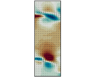
  $\chi$ are triangular at the beginning of the selected time interval, which corresponds to the beating phenomenon that was investigated experimentally and theoretically by Faure-Beaulieu et al. (Reference Faure-Beaulieu, Indlekofer, Dawson and Noiray2021b) for the case of thermoacoustic modes in annular combustion chambers. They showed that this beating of the acoustic amplitude at any point in the cavity is a manifestation of periodic transitions between pure CW and pure CCW spinning waves. These transitions between the pure states are heteroclinic orbits in the phase space, which can be explained by the presence of small asymmetries in the flow or in the system geometry (Faure-Beaulieu et al. Reference Faure-Beaulieu, Indlekofer, Dawson and Noiray2021b).

Figure 3. (a) Measured RMS acoustic pressure at  $\varTheta=0^\circ,\ r=90\ {\rm mm}$, as function of the bulk velocity in the duct. The coloured vertical lines correspond to conditions for which PIV data are available. (b) Detail of acoustic oscillations at six different locations for $U_x=60.3\ {\rm m}\ {\rm s}^{-1}$. (c) Spectrogram of the signal measured in $\varTheta=0^\circ$, $r=90\ {\rm mm}$ for $U_x$ from 0 to $75\ {\rm m}\ {\rm s}^{-1}$. The white line corresponds to the power spectral density shown in panel (d). (d) Power spectral density for $U_x=58.8\ {\rm m}\ {\rm s}^{-1}$ at three azimuthal locations (same colour code as in panel b).

Figure 4. First row: acoustic pressure time traces from three microphones placed at almost equispaced angles. Each column corresponds to a different bulk velocity. Second row: amplitude  $A$ of the azimuthal acoustic mode. Third row: Nature angle $\chi$. The sketch on the right indicates the position of the microphones, with the same colour code as in figure 3(b).
Sequences of 0.1 s of PIV images were acquired for several conditions represented as vertical lines in figure 3(a). The acquisition frequency is 6 kHz, which is sufficient to resolve the hydrodynamic motion at the instability frequency 790 Hz, corresponding to a period of 1.3 ms. The acoustic pressure is measured simultaneously, allowing to investigate the links between acoustics and hydrodynamics. The duration of the PIV measurements is short compared with the 100 s of the acoustic time series, but the images were taken on a representative set of bulk velocities  $U_x$. In figure 4, the dashed black lines materialise the PIV time windows. For these three cases, different behaviours of the acoustic signal are observed during this window. As explained above, these acoustic measurements show that the state of the mode is not constant, but undergoes large temporal fluctuations. For this reason, there are conditions for which several PIV sequences were taken to capture different behaviours at the same operating conditions (three PIV acquisitions were performed for each of the points $U_x = 52.3$, $53.3$ and $59.5$ m s $^{-1}$).
3. Coherent aerodynamics of the axisymmetric shear layer
3.1. Phase-averaged field in the central plane
In figure 1(b), despite the presence of intense turbulent fluctuations, we can identify coherent structures corresponding to vortex shedding along the axisymmetric mean shear layer that forms at the cavity opening, at a radius  $r=20$ mm. However, for the conditions exhibiting weaker aeroacoustic oscillations, the coherent flow motion is less obviously perceptible in instantaneous velocity fields. The classic triple decomposition of the velocity field (Reynolds & Hussain Reference Reynolds and Hussain1972) is now used:
 \begin{equation} \boldsymbol{u}(\boldsymbol{\boldsymbol{x}},t)=\bar{\boldsymbol{u}}(\boldsymbol{\boldsymbol{x}}) + \tilde{\boldsymbol{u}}(\boldsymbol{\boldsymbol{x}},t) + \boldsymbol{u}'(\boldsymbol{\boldsymbol{x}},t), \end{equation}
where  $\bar{\boldsymbol {u}}$ is the time-averaged velocity, $\tilde {\boldsymbol {u}}$ embeds the coherent oscillations associated to the aeroacoustic instability and $\boldsymbol {u}'$, the turbulent fluctuations. The phase-averaged velocity $\langle \boldsymbol {u}\rangle =\bar {\boldsymbol {u}}+ \tilde {\boldsymbol {u}}$ is the velocity field from which turbulent fluctuations have been removed. To obtain this phase-averaged flow from the PIV data, images are grouped in different bins as function of their phase in an acoustic period, and then averaged. In the work of Bourquard et al. (Reference Bourquard, Faure-Beaulieu and Noiray2021), the whistling of a deep cuboid is investigated and the flow can be considered as two-dimensional (2-D). Their 2-D PIV fields reveal a flapping motion of the shear layer at the cavity opening and provide already complete information about the coherent hydrodynamic motion. In the present study, the mean shear layer is cylindrical and a single 2-D cut of the velocity field is not sufficient to describe the velocity fluctuations in the whole cavity, because the amplitude of the oscillation is not necessarily constant along the coordinate $\varTheta$. However, applying phase-averaging in a given plane is still meaningful if the state of the mode does not change during the time interval of the PIV data collection. Therefore, the acoustic data, from which the state variables are extracted, allow for the selection of a portion of the PIV time window over which the state of the mode does not significantly vary. During this time interval, phase averaging was performed and the results are presented in figure 5. The acoustic signal is filtered around the fundamental peak of the instability, its analytical signal is obtained with a Hilbert transform whose phase is used to sort the PIV fields in 12 phase bins. The velocity fields of each bin are averaged to obtain 12 phase-averaged fields. The turbulent fluctuations, not correlated with the coherent motion, are suppressed by the averaging operation. In figures 5(b) to 5(d), the vertical component of the phase-averaged velocity field for $U_x = 58.8\ {\rm m}\ {\rm s}^{-1}$ is presented at the fundamental frequency of the self-sustained aeroacoustic oscillations ( $\,f = 790\ {\rm Hz}$) and at the first and second harmonic frequencies ( $f = 1580\ {\rm Hz}$ and $f = 2370\ {\rm Hz}$). One can see that the amplitude of the coherent oscillations at the fundamental frequency is significantly higher than the one at the harmonics. Figure 5(a) shows amplitude spectra of the instantaneous vertical velocity spatially averaged over a small region of the shear layer for three different operating points: a high amplitude aeroacoustic limit cycle for $U_x = 58.8\ {\rm m}\ {\rm s}^{-1}$, a moderate amplitude aeroacoustic limit cycle for $U_x = 47\ {\rm m}\ {\rm s}^{-1}$, and a linearly stable aeroacoustic condition for $U_x = 41\ {\rm m}\ {\rm s}^{-1}$. The aeroacoustic instability for $U_x = 58.8\ {\rm m}\ {\rm s}^{-1}$ leads to self-sustained oscillations at 790 Hz which can be seen in the PSD of the acoustic pressure (see figure 3d) and in the amplitude spectra of the coherent vertical velocity in the shear layer (see figure 5a). Furthermore, one can see in both figures that harmonics of this fundamental oscillation frequency at 1580 Hz and 2370 Hz are present in the spectral signature of the aeroacoustic self-oscillation, but that their relative magnitude is significantly stronger for the hydrodynamic oscillations of the shear layer than for the acoustic pressure in the cavity. The case of $U_x = 47.0\ {\rm m}\ {\rm s}^{-1}$ is also linearly unstable, but with lower acoustic and hydrodynamic oscillation amplitudes. In figure 3(d), peaks are present at the same frequencies, although the Strouhal number based on the bulk velocity in the pipe is roughly one third lower than for the previous case. This is a manifestation of the fact that in the present configuration, the acoustic eigenmode dictates the frequency of the aeroacoustic limit cycles (see the horizontal bright line in figure 3c), and thus the frequency of the corresponding aerodynamic oscillation. The third case, $U_x = 41\ {\rm m}\ {\rm s}^{-1}$, is aeroacoustically linearly stable and is located close to the Hopf bifurcation ( $U_x \approx 42\ {\rm m}\ {\rm s}^{-1}$), which separates aeroacoustic resonance from aeroacoustic limit cycles (see figure 3d). A piece of striking evidence of the hydrodynamic stability of the shear layer in this case is that there are no visible peaks in the blue amplitude spectrum presented in figure 5(a). Figure 6 shows single snapshots of the phase-averaged cycle for the three components of $\tilde {\boldsymbol{u}}$, at two different flow conditions $U_x=25.9$ m s $^{-1}$ (figure 6a) and $U_x=47.0$ m s $^{-1}$ (figure 6b). These two conditions belong to the two separate instability ranges that have been shown in figures 3(a) and 3(c) and that involve the same acoustic mode at $f\simeq 790$ Hz. The structure of the coherent fluctuations of the longitudinal and transverse velocity components is similar to the coherent velocity fields obtained in whistling 2-D deep cavities (e.g. Bourquard et al. Reference Bourquard, Faure-Beaulieu and Noiray2021; Ho & Kim Reference Ho and Kim2021). The phase-averaging reveals that the hydrodynamic modes involved in the two aeroacoustic instabilities are different. In the second instability range ( $42\ {\rm m\ s}^{-1} < U_x < 73\ {\rm m\ s}^{-1}$), exhibiting the largest acoustic amplitude, the size of the vortices is approximately equal to the cavity's width (figure 6b). This structure will be referred to as the ‘first shear layer mode’. In the first instability range ( $23\ {\rm m\ s}^{-1} < U_x < 33\ {\rm m\ s}^{-1}$), the vortices are smaller and two of them fit in the cavity's span (figure 6a), we refer to this structure as the ‘second shear layer mode’. For both modes, $\tilde{u}_y$ is symmetric with respect to the axis $y=0$ and $\tilde{u}_x$ is antisymmetric ( $\tilde{u}_x(-y) \approx -u_x(y)$), which indicates that the vortices on the opposite sides of the shear layer rotate in the same direction (this is also materialised by the vectors in figure 6). Consequently, these opposite sides move up and down together. This antisymmetric motion indicates that the vortex shedding pattern is not rotationally symmetric, but rather has an odd azimuthal order. Since the azimuthal order of the acoustic mode is 1, the hydrodynamic structure is likely to have the same azimuthal order, although the PIV data does not provide this information. This coincidence between the azimuthal order of the dominant acoustic and hydrodynamic modes can be justified as follows. The velocity field $\tilde {\boldsymbol {u}}$ is assumed to be dominated by a single azimuthal wave number $m\in \mathbb {N}^\ast$:
 \begin{equation} \langle \boldsymbol{u}\rangle(x,r,\varTheta,t)=\bar{\boldsymbol{u}}(x,r) + \tilde{\boldsymbol{u}}^{(m)}(x,r,t)\,{\rm e}^{{\rm i}m\varTheta} + \tilde{\boldsymbol{u}}^{({-}m)}(x,r,t) \,{\rm e}^{-{\rm i}m\varTheta}, \end{equation}
where  $\tilde{\boldsymbol {u}}^{(m)}$ is the amplitude of the $m$th azimuthal component of the coherent fluctuation (and $\tilde{\boldsymbol {u}}^{(-m)}$ its complex conjugate), and where the mean flow $\bar {\boldsymbol {u}}$ is assumed axisymmetric. The associated vorticity is
 \begin{equation} \langle \boldsymbol{\varOmega}\rangle(x,r,\varTheta,t)=\bar{\boldsymbol{\varOmega}}(x,r) + \tilde{\boldsymbol{\varOmega}}^{(m)}(x,r,t)\,{\rm e}^{{\rm i}m\varTheta} + \tilde{\boldsymbol{\varOmega}}^{({-}m)}(x,r,t)\, {\rm e}^{-{\rm i}m\varTheta}. \end{equation}
The acoustic velocity field, dominated by the first azimuthal mode, may be written as
 \begin{equation} \boldsymbol{u}_{ac}(r,x,\varTheta,t)=\boldsymbol{u}_{ac}^{(1)}(r,x,t) \,{\rm e}^{{\rm i} \varTheta} +\boldsymbol{u}_{ac}^{({-}1)} (r,x,t)\,{\rm e}^{-\mathrm{i} \varTheta}. \end{equation}
The acoustic power produced by vorticity fluctuations in a low-Mach flow of mean density  $\bar {\rho }$ in a volume $V$ is given by the Howe's energy corollary (Howe Reference Howe1979):
 \begin{equation} \mathcal{P}={-}\int_V \bar{\rho}(\boldsymbol{\varOmega}\times \boldsymbol{u})\boldsymbol{\cdot}\boldsymbol{u}_{ac}\,{\rm d}V. \end{equation}
It results from the projection of the unsteady component of the Lamb vector  $\boldsymbol {\varOmega }\times \boldsymbol {u}$ onto the acoustic field. In the present case, considering only the contributions of the phase-averaged quantities to the sound production, the expressions (3.2), (3.3) and (3.4) are inserted into (3.5). The integrand contains terms of order $\pm 2m\pm 1$, $\pm m\pm 1$ and $\pm$1. All these terms vanish at the integration over the cavity volume along the azimuthal coordinate $\varTheta$, except the terms $\pm (m-1)$ if $m=1$. This simplified reasoning demonstrates that only azimuthal hydrodynamic modes of order 1 can provide acoustic energy to the first azimuthal acoustic mode. This conclusion is however valid only for negligible azimuthal harmonics of $\tilde {\boldsymbol {u}}$, because interactions between components of different orders can also lead to effective forcing of the first acoustic mode. Formula (3.5) also explains why the first shear layer mode is associated with larger acoustic amplitudes than the second. In the former, each side of the shear layer contains a single vortex, while in the latter, each side contains two counter-rotating vortices whose effects partially cancel out in the integral.
It is interesting to note that the first harmonic of  $\tilde{u}_y$ when the aeroacoustic limit cycle involves the first shear layer mode (see figure 5c) looks similar to the second shear layer mode of figure 6(a), but the former is antisymmetric with respect to the axis, while the latter mode is symmetric. This antisymmetry characterises a hydrodynamic structure of even azimuthal order, most probably of order 0 or 2. The second harmonic of the first shear layer mode (figure 5d) is symmetric, indicating an odd azimuthal order.

Figure 5. (a) Amplitude spectra of the velocity  $\mathcal {U}_y^\mathcal {A}(t)$, which is obtained by spatially averaging the time-resolved vertical velocity fluctuations $\tilde{u}_y$ from PIV over the small region $\mathcal {A}$ of the shear layer defined by $(x,y)\in [3.3;7.3]\times [20;30]$ mm $^2$ shown in (b). Bulk velocities $U_x=58.8$ m s $^{-1}$ (strong instability), $U_x=47.0$ m s $^{-1}$ (moderate instability) and $U_x=41.0$ m s $^{-1}$ (stable) are considered. (b–d) Phase-averaged vertical component of the coherent velocity fluctuations $\tilde{u}_y$ in m s $^{-1}$, at the fundamental frequency and at the first two harmonics, for $U_x=58.8$ m s $^{-1}$.

Figure 6. Phase average of the three components of the coherent velocity fluctuations for (a) an aeroacoustic limit cycle of the first instability range ( $U_x=25.9$ m s $^{-1}$, 790 Hz), which involves the second shear layer mode, and (b) an aeroacoustic limit cycle of the second instability range ( $U_x=47.0$ m s $^{-1}$, 784 Hz), which involves the first shear layer mode.
3.2. Volumetric coherent aerodynamics during spinning states
Figure 7(a) shows the cycle of  $\langle u_x\rangle$ at $U_x = 60.3\ {\rm m}\ {\rm s}^{-1}$, showing vortical structures convected along the shear layer from left to right across the cavity aperture. Although it is, in general, impossible to reconstruct the whole three-dimensional (3-D) phase-averaged velocity field from the 2-D PIV slices, it can be achieved for pure spinning modes, because they are characterised by a velocity and pressure field that rotates around the axis with constant amplitude, which means that identical sequences would be obtained by considering the temporal evolution of a 2-D slice of $\langle \boldsymbol {u} \rangle$ at constant $\varTheta$, or by freezing the time and moving the angle $\varTheta$ of the 2-D slice against the wave's direction of propagation. Since PIV gives access to the temporal evolution of $\langle \boldsymbol {u} \rangle$ at constant $\varTheta$, the whole 3-D phase-averaged velocity field can be reconstructed for a spinning mode, as done by Oberleithner et al. (Reference Oberleithner, Sieber, Nayeri, Paschereit, Petz, Hege, Noack and Wygnanski2011) for a swirling jet. The reconstruction is applied for the case of $U_x = 60.3$ m s $^{-1}$, which is very close to a pure spinning CW aeroacoustic wave, and whose state does not significantly change during the PIV time interval. Figure 7(b) shows several representations of the 3-D reconstructed coherent velocity field. The first (left) is an isosurface of the whole phase-averaged axial velocity field $\langle u_x \rangle$. Although $\bar {u}_x$ is large, the coherent perturbations $\tilde{u}_x$ are not negligible compared with the mean and make a visible spiral wave on the isosurface. The third image from the left shows one positive and one negative isosurface of the coherent radial velocity fluctuations, that take the shape of two spiralling crescents. The rightmost image shows a positive isosurface of the $Q$-criterion (Jeong & Hussain Reference Jeong and Hussain1995), highlighting the spiralling vortex tube detaching from the edge of the cavity opening. One can now elaborate on the physics of the helical structure of the mode shown in figure 7(b), which is especially visible in the $Q$-criterion isosurface representation. The blue arrow indicates the direction of the acoustic wave, spinning in the opposite direction to the winding of the spiral, which can be explained by the following mechanism: when the acoustic wave spins around the cavity, the radial component of the travelling acoustic velocity perturbation governs a continuous vortex shedding along at the upstream edge of the cavity opening. The combination of this spinning perturbation and the advection of the resulting vortex tube causes naturally a spiral winding against the direction of the perturbation. Reciprocally, looking from a fixed axial position at the advection of the helical vortex tube, we observe vorticity perturbations spinning against the winding of the spiral. This is simply a geometrical property of an infinite constant pitch spiral: a translation along the axis is equivalent to a rotation in the opposite direction with respect to the winding. These spinning vorticity fluctuations are sound sources that govern the aeroacoustic limit cycle. In summary, in our configuration, negative helical modes are associated with CW spinning waves, and positive helical modes with CCW waves, following the terminology used by Gallaire & Chomaz (Reference Gallaire and Chomaz2003). In the next section we discuss the emergence of a non-zero azimuthal mean flow, although the incoming pipe flow is purely axial, i.e. without swirl. The red arrow on figure 7(b) represents the direction of this self-induced swirl. The helical mode is co-winding and counter-spinning with respect to the self-induced swirl, with the definition of ‘co-winding’ usually used in the literature on swirled flows (e.g. Oberleithner, Paschereit & Wygnanski Reference Oberleithner, Paschereit and Wygnanski2014). The link between the swirl, the winding direction and the spinning direction of the helix will be discussed in Reference Faure-Beaulieu, Pedergnana and NoirayPart 2 of the present study.

Figure 7. Phase average of centreplane velocity fields from stereoscopic PIV and 3-D reconstructed field for the condition  $U_x=60.3$ m s $^{-1}$ when the aeroacoustic limit cycle corresponds to a quasi-pure spinning mode. (a) Phase average sequence. (b) Isosurfaces of the 3-D reconstruction of the flow oscillations and the $Q$ criterion. The red arrow indicates the direction of the self-induced azimuthal mean flow direction during the PIV time window. The blue arrow shows the spinning direction of the acoustic wave. (c) Axial, radial and azimuthal components of the 3-D reconstructed field of the coherent velocity fluctuations in the central y–z plane. An animated 3-D reconstruction of the 3-D coherent field is provided as supplementary material (see supplementary movies 1–4 available at https://doi.org/10.1017/jfm.2023.352) for the different conditions.
4. Symmetry breaking of the mean flow by spinning waves
4.1. Evidence of the emergence of a mean azimuthal flow
In the PIV fields corresponding to the largest aeroacoustic oscillations, a non-zero mean flow is present in the out-of-plane direction  $z$. Figure 8(a,b) shows examples of this mean flow for $U_x=47.0$ m s $^{-1}$, corresponding to a CW spinning mode of moderate amplitude ( $p\sim 0.8$ kPa) and $U_x=60.3$ m s $^{-1}$, corresponding to a CW spinning mode of large amplitude ( $A\sim 5$ kPa). The averaging was performed over the 0.1 s of the PIV acquisition (600 images), but averaging over shorter time intervals of 8.3 ms (50 images) give a similar velocity field. The fields are antisymmetric with respect to the axis, indicating a swirling motion. For $U_x=60.3$ m s $^{-1}$, $\overline {u_\varTheta }$ reaches 10 m s $^{-1}$ at the position of the shear layer ( $r=20$ mm), corresponding to 8 revolutions during the 0.1 s of measurement, which is 10 times slower than the aeroacoustic wave, spinning 79 times around the cavity in the same duration. The two mean flows whirl CCW in the shear layer and have a weak core rotating in the opposite direction in the centre. The experimental results indicate that this quasi-steady self-induced swirling flow is linked to the presence of an intense aeroacoustic wave spinning in the cavity because it is no longer observed when the system is aeroacoustically stable ( $33\ {\rm m}\ {\rm s}^{-1} < U_x < 42\ {\rm m}\ {\rm s}^{-1}$). Moreover, the whirling direction is correlated with the spinning direction of the aeroacoustic wave, as shown in the next paragraph.

Figure 8. Out-of-plane component  $\bar {u}_z$ of the experimental mean flow for (a) $U_x = 47.0$ m s $^{-1}$ and (b) $U_x = 60.3$ m s $^{-1}$. The domain $\mathcal {S}_1$ is defined by $0\leq y \leq 38$ mm, $\mathcal {S}_2$ is defined by $-38\ {\rm mm}\leq y \leq 0$. (c) Fluctuations of the spatially averaged azimuthal mean flow, for $U_x = 60.3$ m s $^{-1}$. Black line: Instantaneous fluctuations. Red line: Moving average over 8.3 ms (50 time steps of the PIV).
To study the behaviour of the azimuthal flow, we define  $U_\varTheta (t)$ as a spatial average of $u_z(x,y,t)$ over the PIV window for $0\leq r\leq 38$ mm. This is done by computing the averages of $u_z$ weighted by $y$ over the domains $\mathcal {S}_1$ (above the axis) and $\mathcal {S}_2$ (below the axis) represented in figure 8(b), and subtracting the latter from the former, to account for the change of orientation of the unit vector $\boldsymbol {e}_\varTheta$ below the axis. The temporal evolution of $U_\varTheta (t)$ for the case of $U_x=60.3$ m s $^{-1}$ is represented in figure 8(c) (black line), showing oscillations around a positive value corresponding to a predominantly CCW whirling direction. Despite the spatial averaging, irregular oscillations are clearly visible, due to the turbulent and coherent velocity fluctuations. These fluctuations are eliminated by applying a moving average of 8.3 ms (red line), giving a smooth evolution of $U_\varTheta$ on slow time scales with respect to the acoustic oscillations. Figure 9(d) shows the smoothed temporal evolution of $U_\varTheta$ for all the operating conditions in the second azimuthal instability range and for which PIV images are available (the colour codes are the same as in figure 3a). Figure 9(a) shows the trajectory of the nature angle $\chi$ as function of $U_\varTheta$ for the same set of operating conditions. Although these individual trajectories look rather erratic at first glance, they are all located in the regions ( $\chi >0, U_\varTheta <0$) and ( $\chi <0, U_\varTheta >0$); the two other quadrants are quasi-empty: the acoustic wave and the quasi-steady swirl mostly spin in opposite directions. Figure 9(c) shows the evolution of $\chi$ over a PIV time window. Since $\chi$ can have significant variations over an interval of 0.1 s, the time window is split into five time intervals $\Delta t$ during which the variations remain limited. Figure 9(b) shows the mean value of $\lvert U_\varTheta \rvert$ as a function of the rate of change of $\chi$ over each of these short time slots $\Delta t$. This scatter plot has the shape of a triangle whose base lies on the axis $\lvert U_\varTheta \rvert =0$ and whose top is on the axis $\Delta \chi /\Delta t=0$. This reveals that stronger swirl is associated with cases where $\chi$ varies little. In addition, the size of the circles in figure 9(b) is proportional to the acoustic pressure. One sees that the points with the largest bulk azimuthal velocity $U_\varTheta$, i.e. the strongest swirl, correspond also to the largest acoustic levels. These observations could be explained as follows: when an azimuthal aeroacoustic wave of sufficiently large amplitude spins in a certain direction during a sufficient amount of time, the large hydrodynamic velocity fluctuations lead to the development of a mean flow spinning in the opposite direction. On the other hand, when the aeroacoustic wave constantly changes its spinning direction, the mean swirl does not have sufficient time to establish in a given direction. A second possible explanation could be that the swirl appears first, as a spontaneous symmetry breaking of the mean flow, and then influences the spinning direction of the wave and its amplitude. However, this alternative interpretation does not explain how a swirling motion spontaneously appears only for a small range of bulk axial flow velocity $U_x$. A third possible explanation could involve acoustic streaming: a large-amplitude acoustic travelling wave can indeed induce a net mean flow in a closed loop system (Gedeon Reference Gedeon1997; Boluriaan & Morris Reference Boluriaan and Morris2003). The Mach $M_{in}$ of the induced mean flow is of the order of the square of the acoustic mach number $M_{ac}=u_\text a/c$, where $c$ is the speed of sound and $u_\text a$, the typical amplitude of the acoustic velocity oscillations: $M_{in} \sim u_a^2/c^2 \sim p_a^2/(\rho ^2 c^4)=0.0014$ in the case of an acoustic pressure wave of amplitude 5 kPa, corresponding to an azimuthal velocity of 0.5 m s $^{-1}$ approximately, which cannot explain the higher values observed in figures 8 and 9d). In the following sections, the validity of the first explanation is confirmed with a linear perturbation analysis, showing that the hydrodynamic component of the aeroacoustic limit cycle can indeed induce symmetry breaking of the mean flow.

Figure 9. (a) Trajectories of the slowly evolving azimuthal flow as a function of the nature angle  $\chi$, showing evidence that the mean flow tends to spin in the opposite direction compared with the acoustic wave. (b) Scatter plot of the azimuthal flow in function of the variation rate of $\chi$, showing that the highest azimuthal mean flows are obtained when $\chi$ does not vary much. The radii of the circles corresponds to the amplitude of the acoustic pressure oscillations. (c,d) Temporal evolution of $\chi$ and $U_\varTheta$ over the PIV time window. The colour code corresponds to the axial bulk velocity. The line with a dashed border corresponds to the case $U_x=60.3$ m s $^{-1}$ shown in figure 7.
4.2. Linear modal analysis
The experimental measurements are not sufficient to unravel the mechanisms that lead to the emergence of a mean swirling flow in a symmetric cavity. This is why we supplement them with a theoretical and numerical study of the hydrodynamic oscillations. To do so, an approach based on linearised Navier–Stokes equations (LNSE) is adopted. This method has been used since decades to study the linear stability of a flow and to identify the main hydrodynamic structures and their associated growth rates and frequencies (Jackson Reference Jackson1987; Natarajan & Acrivos Reference Natarajan and Acrivos1993; Delbende, Chomaz & Huerre Reference Delbende, Chomaz and Huerre1998). The LNSE has been also applied to compute the adjoint sensitivity of these modes to modifications of the flow or the geometry, allowing the development of passive control strategies (Hill Reference Hill1992; Marquet, Sipp & Jacquin Reference Marquet, Sipp and Jacquin2008). This application of LNSE is promising for engineering applications and was successfully adapted for compressible flows (Meliga, Sipp & Chomaz Reference Meliga, Sipp and Chomaz2010), turbulent flows (Meliga, Pujals & Serre Reference Meliga, Pujals and Serre2012; Tammisola & Juniper Reference Tammisola and Juniper2016) and complex swirling flows (Qadri, Mistry & Juniper Reference Qadri, Mistry and Juniper2013; Tammisola & Juniper Reference Tammisola and Juniper2016). The LNSE analysis is also valuable to study the phenomenon of non-normal growth observed in a wide range of stable flows (Farrell & Ioannou Reference Farrell and Ioannou1996; Chomaz Reference Chomaz2005) which act as noise amplifiers and react strongly to harmonic excitation around certain frequencies (Garnaud et al. Reference Garnaud, Lesshafft, Schmid and Huerre2013; Sipp & Marquet Reference Sipp and Marquet2013) or stochastic forcing (Boujo & Gallaire Reference Boujo and Gallaire2015), and which show transient energy growths although they are linearly stable. Moreover, compressible LNSE approaches also give information on the aeroacoustic noise produced by hydrodynamic instabilities (Beneddine, Mettot & Sipp Reference Beneddine, Mettot and Sipp2015; Fani et al. Reference Fani, Citro, Giannetti and Auteri2018). Yamouni, Sipp & Jacquin (Reference Yamouni, Sipp and Jacquin2013) used this approach to assess the stability of the full aeroacoustic feedback loop of a 2-D cavity flow.
Given the intrinsic nonlinear nature of fluid motion, the following key question arises: Which steady flow should be considered for investigating linear evolution of small perturbations? Early studies on the unstable cylinder wake showed that a linear perturbation analysis on the steady solution of the Navier–Stokes equations, the so-called base flow, does not provide a reliable estimation of the instability's frequency and structure far away from the critical Reynolds number, while a linear perturbation analysis on the mean flow gives an excellent agreement (Pier Reference Pier2002; Barkley Reference Barkley2006). Later, Sipp & Lebedev (Reference Sipp and Lebedev2007) and Turton, Tuckerman & Barkley (Reference Turton, Tuckerman and Barkley2015) provided a mathematical ground to this mean flow approach. These studies also demonstrated that the linear perturbation analysis on the mean flow is valid only in the absence of strong nonlinear interactions between the fundamental hydrodynamic mode and its harmonics.
Numerous studies applied LNSE analysis on turbulent mean flows, and give insightful results about the main hydrodynamic modes of various flows and their response frequency (e.g. Monkewitz Reference Monkewitz1988; del Álamo & Jiménez Reference del Álamo and Jiménez2006; Meliga, Sipp & Chomaz Reference Meliga, Sipp and Chomaz2009; Iungo et al. Reference Iungo, Viola, Camarri, Porté-Agel and Gallaire2013; Gikadi, Föller & Sattelmayer Reference Gikadi, Föller and Sattelmayer2014; Oberleithner, Schimek & Paschereit Reference Oberleithner, Schimek and Paschereit2015; Tammisola & Juniper Reference Tammisola and Juniper2016; Boujo et al. Reference Boujo, Bauerheim and Noiray2018). As stated by Beneddine et al. (Reference Beneddine, Sipp, Arnault, Dandois and Lesshafft2016), the linearised approach on a turbulent mean flow can be particularly relevant when the dynamics are dominated by a strong convective instability mechanism, which is the case in shear layer flows.
While the issue of the choice of mean flow will be further discussed later, let us now present the LNSE analysis, which will allow us to identify the dominant hydrodynamic modes and to compare them with the experimental observations. Later, we show that the main LNSE mode is able to generate a swirling flow. Incompressible Navier–Stokes equations are here sufficient to describe the hydrodynamic modes at the instability frequency because the Mach number of the flow is low and the thickness of the shear layer ( ${\sim}0.01$ m) and its length (0.03 m) are short compared with the acoustic wavelength at 790 Hz, which is about 0.4 m. Therefore, the acoustic phase can be considered as constant over the shear layer region. The incompressible Navier–Stokes equations are
 \begin{equation} \begin{cases} \dfrac{\partial \boldsymbol{u}}{\partial t} + \boldsymbol{u}\boldsymbol{\cdot} \boldsymbol{\nabla} \boldsymbol{u} + \dfrac{1}{\rho}\boldsymbol{\nabla} p -\nu \nabla^2 \boldsymbol{u} = 0,\\ \boldsymbol{\nabla}\boldsymbol{\cdot} \boldsymbol{u} =0, \end{cases} \end{equation}
where  $\nu$ is the kinematic viscosity. After introducing the triple decomposition (3.1) into (4.1) and performing time-averaging, the RANS equations are obtained:
 \begin{equation} \begin{cases} \boldsymbol{\bar{u}}\boldsymbol{\cdot}\boldsymbol{\nabla} \bar{\boldsymbol{u}} + \overline{\tilde{\boldsymbol{u}}\boldsymbol{\cdot}\boldsymbol{\nabla} \tilde{\boldsymbol{u}}} + \overline{\boldsymbol{u}'\boldsymbol{\cdot}\boldsymbol{\nabla} \boldsymbol{u}'} + \dfrac{1}{\rho}\boldsymbol{\nabla} \bar p -\nu \nabla^2 \bar{\boldsymbol{u}} = 0,\\ \boldsymbol{\nabla}\boldsymbol{\cdot} \bar{\boldsymbol{u}} =0. \end{cases} \end{equation}
Then, phase averaging is applied to (4.1), and (4.2) is subtracted to it to obtain the equations for the coherent fluctuations:
 \begin{equation} \begin{cases} \dfrac{\partial \tilde{\boldsymbol{u}}}{\partial t} + \bar{\boldsymbol{u}}\boldsymbol{\cdot}\boldsymbol{\nabla} \tilde{\boldsymbol{u}}+ \tilde{\boldsymbol{u}}\boldsymbol{\cdot}\boldsymbol{\nabla} \bar{\boldsymbol{u}} + \widetilde{\boldsymbol{u}'\boldsymbol{\cdot}\boldsymbol{\nabla} \boldsymbol{u}'} + \widetilde{\tilde{\boldsymbol{u}}\boldsymbol{\cdot}\boldsymbol{\nabla} \tilde{\boldsymbol{u}}} + \dfrac{1}{\rho}\boldsymbol{\nabla} \tilde{p} -\nu \nabla^2 \tilde{\boldsymbol{u}} = 0,\\ \boldsymbol{\nabla}\boldsymbol{\cdot}\tilde{\boldsymbol{u}}=0. \end{cases} \end{equation}
With the incompressibility assumption in the shear layer region ( $\boldsymbol {\nabla }\boldsymbol{\cdot}\bar {\boldsymbol {u}}=\boldsymbol {\nabla }\boldsymbol{\cdot}\tilde {\boldsymbol {u}}=\boldsymbol {\nabla }\boldsymbol{\cdot}\boldsymbol {u}'=0$), the coherent nonlinear advection terms $\widetilde {\boldsymbol {u}'\boldsymbol{\cdot}\boldsymbol {\nabla } \boldsymbol {u}'}$ and $\widetilde {\tilde {\boldsymbol {u}}\boldsymbol{\cdot}\boldsymbol {\nabla } \tilde {\boldsymbol {u}}}$ simplify to $\boldsymbol {\nabla }\widetilde {\boldsymbol {u}' \boldsymbol {u}'}$ and $\boldsymbol {\nabla }\widetilde {\tilde {\boldsymbol {u}}\tilde {\boldsymbol {u}}}$, respectively. Herewith, the influence of the coherent component of the turbulent Reynolds stress tensor $\widetilde {\boldsymbol {u}' \boldsymbol {u}'}$ upon the coherent dynamics has to be modelled in order to achieve the linear perturbation analysis. To do so, we use the Boussinesq assumption, considering that turbulent fluctuations diffuse along the gradient of the mean velocity, which has shown to give reliable results on various flows in past studies (e.g. Viola et al. Reference Viola, Iungo, Camarri, Porté-Agel and Gallaire2014; Tammisola & Juniper Reference Tammisola and Juniper2016; Boujo et al. Reference Boujo, Bauerheim and Noiray2018):
 \begin{equation} -\widetilde{\boldsymbol{u}'\boldsymbol{u}'}+\tfrac{2}{3}\tilde{k}\textbf{I} = \nu_t (\boldsymbol{\nabla} + \boldsymbol{\nabla}^\top)\tilde{\boldsymbol{u}}, \end{equation}
where  $\tilde{k}=\widetilde {\boldsymbol {u}'\boldsymbol{\cdot}\boldsymbol {u}'}/2$ is the coherent component of the turbulent kinetic energy, $\textbf{I}$ is the identity matrix and $\nu _t$ is the turbulent viscosity for the coherent fluctuations, which can be extracted from unsteady experimental or LES data by locally linking the mean turbulent Reynolds stress tensor $\overline {\boldsymbol {u}'\boldsymbol {u}'}$ and the mean strain rate tensor $\overline {\boldsymbol S}=(\boldsymbol {\nabla } + \boldsymbol{\nabla}^\top )\bar{\boldsymbol{u}}$, as explained by Rukes, Paschereit & Oberleithner (Reference Rukes, Paschereit and Oberleithner2016). Alternatively, $\nu _t$ can be directly obtained from a simulation relying on a turbulent viscosity model, for instance a RANS $k-\omega$ model. Taking the divergence of (4.4) and using the incompressibility of the flow ( $\boldsymbol {\nabla } \boldsymbol{\cdot}\bar {\boldsymbol {u}}=0, \boldsymbol {\nabla } \boldsymbol{\cdot} \boldsymbol {u}'=0$), one finds
 \begin{equation} \boldsymbol{\nabla}\boldsymbol{\cdot}\widetilde{\boldsymbol{u}'\boldsymbol{u}'}={-}\nu_t \boldsymbol{\nabla}^2\tilde{\boldsymbol{u}} - \boldsymbol{\nabla} \nu_t^\top \boldsymbol{\cdot} (\boldsymbol{\nabla} \tilde{\boldsymbol{u}} + \boldsymbol{\nabla} \tilde{\boldsymbol{u}} ^\top) + (2/3)\boldsymbol{\nabla} \tilde{k}\textbf{I}. \end{equation}
As in, e.g., Kitsios et al. (Reference Kitsios, Cordier, Bonnet, Ooi and Soria2010), Viola et al. (Reference Viola, Iungo, Camarri, Porté-Agel and Gallaire2014) or Tammisola & Juniper (Reference Tammisola and Juniper2016), the coherent oscillations are assumed to affect the distribution of the turbulence but not its energy, so  $\tilde{k}=0$. The oscillations of $\nu _t$ are also neglected. The diffusion terms $-\nu _t \boldsymbol {\nabla}^2\tilde {\boldsymbol {u}}$ and $-\nu \boldsymbol {\nabla}^2\tilde {\boldsymbol {u}}$ sum up in (4.3), giving a total effective viscosity $\nu +\nu _t$. In the turbulent regime, $\nu _t\gg \nu$. Indeed, $\nu _t$ extracted from the experiments is of the order of $10^{-3}$ m $^2$ s $^{-1}$ in the shear layer, while $\nu \sim 1.5\times 10^{-5}$ m $^2$ s $^{-1}$.
Next, we consider only the coherent oscillations at one single angular frequency  $\omega$, the fundamental aeroacoustic frequency, and neglect the effect of the harmonics at $2\omega$ and $3\omega$, although they are visible in figure 5. This assumption can only be made in the linear regime and its validity will be further discussed later. The angular frequency $\omega$ is defined as complex: its real part corresponds to the aeroacoustic angular frequency and its imaginary part to a growth rate. The Fourier series of $\tilde {\boldsymbol {u}}$ and $\tilde{p}$ in the azimuthal direction are written as
 $$\begin{gather} \tilde{\boldsymbol{u}}(x,r,\varTheta,t) = \tfrac{1}{2} \sum_{m\in\mathbb{Z}} \hat{\boldsymbol{u}}^{(m)}(x,r)\,\mathrm{e}^{\mathrm{i}(\omega t +m\varTheta)} + \text{c.c.}, \end{gather}$$
 $$\begin{gather}\tilde{p}(x,r,\varTheta,t) = \tfrac{1}{2} \sum_{m\in\mathbb{Z}} \hat{p}^{(m)}(x,r)\,\mathrm{e}^{\mathrm{i}(\omega t +m\varTheta)} + \text{c.c.} , \end{gather}$$
where c.c. denotes ‘complex conjugate’,  ${\rm Re}(\omega )\geq 0$ and the 2-D fields $\hat {\boldsymbol {u}}^{(m)}$ and $\hat p^{(m)}$ are complex, with substantial variations of the phase along the shear layer, which is not compact with respect to the hydrodynamic wavelength. The azimuthal orders $m>0$ (respectively, $m<0$) corresponds to waves spinning in the CW (respectively, CCW) direction. By truncating (4.6) and (4.7) at order 1, the task of writing (4.3) in the frequency domain at the fundamental frequency is simplified, because $\boldsymbol {\nabla } \boldsymbol{\cdot } \tilde {\boldsymbol {u}}\tilde {\boldsymbol {u}}$ contains only terms at frequencies 0 and $2\omega$, so it does not contribute directly to the oscillations at the fundamental frequency. The steady component of $\boldsymbol {\nabla } \boldsymbol{\cdot } \tilde {\boldsymbol {u}}\tilde {\boldsymbol {u}}$ indirectly contributes to the oscillation at the fundamental frequency through its impact on the mean flow. As it will be discussed at the end of § 4.3, such an effect can only be considered with a self-consistent approach, which is not in the scope of the present framework. Once the perturbations described with (4.6) have been introduced into (4.3), it is multiplied with $\mathrm {e}^{-\mathrm {i} m\varTheta }$ and integrated over the circumference to isolate only terms of order $m$. The mean flow being axisymmetric, the terms $\bar {\boldsymbol {u}}\boldsymbol{\cdot}\boldsymbol {\nabla } \tilde {\boldsymbol {u}}$ and $\tilde {\boldsymbol {u}}\boldsymbol{\cdot}\boldsymbol {\nabla } \bar {\boldsymbol {u}}$ in (4.3) are also of order $m$. Consequently, the LNSE in the frequency domain for the components of azimuthal order $m$ are
 \begin{equation} \begin{cases}
\bar{\boldsymbol{u}}\boldsymbol{\cdot}\boldsymbol{\nabla}_m
\hat{\boldsymbol{u}}^{(m)}
+\hat{\boldsymbol{u}}^{(m)}\boldsymbol{\cdot}\boldsymbol{\nabla}_0
\bar{\boldsymbol{u}} + \dfrac{1}{\rho}\boldsymbol{\nabla}_m \hat
p^{(m)}\\ \quad - (\nu + \nu_t) \boldsymbol{\nabla}^2_m
\hat{\boldsymbol{u}}^{(m)} - \boldsymbol{\nabla} \nu_t^\top
\boldsymbol{\cdot} (\boldsymbol{\nabla}_m \hat{\boldsymbol{u}}^{(m)} +
\boldsymbol{\nabla}_m \hat{\boldsymbol{u}}^{(m)\top})
={-}\mathrm{i}\omega\hat{\boldsymbol{u}}^{(m)},\\
\boldsymbol{\nabla}_m\boldsymbol{\cdot} \hat{\boldsymbol{u}}^{(m)}=0,
\end{cases} \end{equation}
\begin{equation} \begin{cases}
\bar{\boldsymbol{u}}\boldsymbol{\cdot}\boldsymbol{\nabla}_m
\hat{\boldsymbol{u}}^{(m)}
+\hat{\boldsymbol{u}}^{(m)}\boldsymbol{\cdot}\boldsymbol{\nabla}_0
\bar{\boldsymbol{u}} + \dfrac{1}{\rho}\boldsymbol{\nabla}_m \hat
p^{(m)}\\ \quad - (\nu + \nu_t) \boldsymbol{\nabla}^2_m
\hat{\boldsymbol{u}}^{(m)} - \boldsymbol{\nabla} \nu_t^\top
\boldsymbol{\cdot} (\boldsymbol{\nabla}_m \hat{\boldsymbol{u}}^{(m)} +
\boldsymbol{\nabla}_m \hat{\boldsymbol{u}}^{(m)\top})
={-}\mathrm{i}\omega\hat{\boldsymbol{u}}^{(m)},\\
\boldsymbol{\nabla}_m\boldsymbol{\cdot} \hat{\boldsymbol{u}}^{(m)}=0,
\end{cases} \end{equation}
where every occurrence of the partial derivative  $\partial /\partial \varTheta$ was replaced by a multiplication with $\mathrm {i} m$ in the spatial differential operator that is now denoted $\boldsymbol{\nabla}_m$. If the harmonics at $k\omega$ with $k\geq 2$ are kept in the expressions (4.6) and (4.7) for $\tilde {\boldsymbol {u}}$ and $\tilde{p}$, (4.8) includes additional terms at order $m$ and angular frequency $\omega$, which originate from nonlinear interactions between the harmonics. Notably, the term resulting from the interaction between the fundamental and the first harmonic has a non-negligible forcing amplitude and one may wonder if it is valid to neglect it. To answer this question, one can refer to the work of Boujo et al. (Reference Boujo, Bauerheim and Noiray2018), who investigated the 2-D counterpart of the present axisymmetric cavity and who showed that the forcing from this nonlinear term, which is mostly distributed around the downstream corner of the cavity, barely affects the motion of the shear layer, which is mostly responsive to perturbations located at the upstream corner of the cavity. Assuming that the flow studied in the present axisymmetric geometry has the same property, the effect of the harmonic on the structure of the fundamental is here neglected. Equation (4.8) is written compactly as
 \begin{equation} L(\bar{\boldsymbol{u}})^{(m)}\hat{\boldsymbol{q}}^{(m)} ={-}\mathrm{i}\omega\hat{\boldsymbol{q}}^{(m)},\end{equation}
where  $\hat {\boldsymbol {q}}^{(m)}=(\hat {\boldsymbol {u}}^{(m)},\hat p^{(m)})$ and $L(\bar {\boldsymbol {u}})^{(m)}$, the LNS operator, is a linear differential operator that depends on the mean flow and the selected azimuthal order $m$.
$m$.
Equation (4.9) is a linear eigenvalue problem of infinite dimension, which can be solved numerically as a finite-dimensional problem by discretising it with finite elements, provided that the mean flow is known. This brings us to the following essential question: Which mean flow  $\bar {\boldsymbol {u}}$ should be used for this linearised perturbation analysis?
For such an investigation, it is of interest to use the mean flow at the onset of the aeroacoustic instability – and not the one of the aeroacoustic limit cycles – which exhibits a shear layer thickened by the stable high-amplitude self-sustained oscillations. This mean flow could be experimentally observed by suddenly turning off a control system counteracting the natural feedback between the acoustic modes of the cavity and the unsteady vorticity of the shear layer. For instance, an active control method based on microphone sensing and loudspeaker actuation, such as the one employed by Noiray & Denisov (Reference Noiray and Denisov2017) in the context of thermoacoustic instabilities, could be used for this purpose. A passive control approach based on sound-absorbing foam placed at the outer wall of the cavity for suppressing azimuthal and radial acoustic modes could also be employed, but it would have the major disadvantage of obstructing the optical access for PIV measurements. Alternatively, this mean flow can be obtained from numerical simulations of the incompressible RANS equations, which are inherently free from the compressible acoustic oscillations. The RANS simulations have the additional advantage of providing the mean flow in the whole cavity–pipe system, while the PIV data are only available in a limited field of view. This numerical approach is adopted in the present work.
Figures 10(a) and 10(b) show the velocity components of the 2-D axisymmetric mean flow computed with a steady incompressible  $k-\omega$ SST RANS simulation using the solver Ansys Fluent for $U_x = 41\ {\rm m}\ {\rm s}^{-1}$. The computational domain extends 70 cm before the cavity and 15 cm after it. A mesh of 38 208 quadrilateral elements is used. The cells in the bulk of the pipe have a typical size of 1 mm. At the walls, inflation layers are used to ensure a good resolution of the turbulent boundary layer profile. In particular, the thickness of the first layer is $1.5\times 10^{-5}$ in the pipe and $5\times 10^{-5}$ in the cavity, giving values of $y^+ \in [0.02,1]$ everywhere except at the cavity's downstream corner, where it locally reaches 3. A uniform velocity inlet profile $U_x$ is imposed at the inlet. Second-order numerical schemes are used for all the transport equations. A mesh convergence study was performed on a coarser mesh (20 774 elements, typical cell size 1.6 mm) and a finer mesh (65 138 elements, typical cell size 0.7 mm). The relative error between the velocity profiles obtained for finer mesh and the normal mesh is smaller than 0.1 % in the shear layer. Three different bulk flow velocities were considered: $U_x=47$, $41$ and $26$ m s $^{-1}$. The case of $U_x=47$ m s $^{-1}$ corresponds to the experimental results presented in figure 6(b), which is, in reality, a condition leading to an aeroacoustic limit cycle involving the first hydrodynamic mode. The case $U_x=41$ m s $^{-1}$ corresponds to the last aeroacoustically stable point before the second instability range. The case $U_x=26$ m s $^{-1}$ corresponds to an aeroacoustic limit cycle involving the second shear layer mode, represented in figure 6(a). Figure 10(c) shows that the experimental and simulated velocity profiles are in very good agreement for $U_x=41$ m s $^{-1}$. Such validation of the RANS simulations is not possible for the two other cases because the experimental mean flow is altered by the aeroacoustic oscillations which cannot develop in the employed incompressible RANS description. Figure 10(d) compares the turbulent viscosity profiles from the incompressible RANS and the ones extracted from the PIV data. Significant differences are found between the shapes of these profiles but the maximum values are well reproduced by the simulation. It was verified that these discrepancies have little effect on the frequency and the structure of the dominant LNSE modes, as in the study of Boujo et al. (Reference Boujo, Bauerheim and Noiray2018). For the following stability analysis based on the incompressible LNSE, the $\nu _t$ field used in (4.8) is the one obtained from the incompressible RANS simulations. In the present work, the steady solutions of the incompressible RANS equations are referred to as ‘base flows’, although this terminology is generally used for steady solutions of the Navier–Stokes equations.

Figure 10. The 2-D axisymmetric incompressible RANS mean flow for  $U_x=41$ m s $^{-1}$, corresponding to a linearly stable aeroacoustic condition between the two separate instability ranges of figure 3(a). As there are no self-sustained coherent oscillations at this condition (see figure 5a) and that the zero-mean fluctuations originate from turbulence, this incompressible simulation can be validated with the PIV data. (a) Axial velocity; (b) radial velocity; (c) $\bar {u}_x$ profiles at axial locations $x = -10, -5, 0, 5$ and 10 mm from RANS (dashed) and PIV (solid line); and (d) turbulent viscosity profiles (dashed lines, RANS; solid lines, PIV).
Solving the eigenvalue problem (4.9) for this base flow allows us to identify which hydrodynamic structures are the most prone to efficiently respond to the harmonic forcing of the acoustic mode. This can be done for each azimuthal order  $m$, but in the present paper, we will focus on $m=\pm 1$, because we investigate aeroacoustic modes of azimuthal order 1. With the finite-element code FreeFem++, the LNS operator was discretised for each of the three base flows and for different values of the azimuthal orders, and especially for $m=1$ and $m=-1$. A weak formulation of the LNSE in cylindrical coordinates is provided in Appendix A. Velocity and pressure fluctuations were respectively discretised with P2 and P1 Taylor–Hood elements. The discretisation gives a generalised eigenvalue problem $Av=\lambda Bv$ with $A$ the matrix of the LNS operator and $B$ the mass matrix. Here $A$ and $B$ are large sparse matrices and a subset of their eigenvalues is found with the Schur method applied on a shift invert of $A$. Since the problem is non-Hermitian, the eigenvalues can be complex and are written as $\lambda =-\mathrm {i}\omega =-\mathrm {i}(2{\rm \pi} f + \mathrm {i}\sigma )$ with $\omega$ the complex angular frequency, $f$ the real frequency and $\sigma$ the real growth rate. In the adopted convention, $\sigma <0$ corresponds to linearly stable eigenmodes, and $\sigma >0$ to linearly unstable eigenmodes. Figure 11 shows the eigenvalues found for the three different base flows for the azimuthal order $m=1$ (CW spinning perturbations). The axisymmetric modes $m=0$ and azimuthal modes of order $m=2$ are also represented in light grey. The LNSE eigenspectra shown in figure 11 for $m=1$ are comparable to the results of Boujo et al. (Reference Boujo, Bauerheim and Noiray2018), which were obtained for the 2-D geometrical counterpart of the present axisymmetric configuration: most of the eigenvalues lie on continuous branches of modes with high damping (in blue), and two isolated modes are located above the branches and are highlighted in red in figure 11. The eigenmode associated with the isolated eigenvalue having the lowest (respectively, highest) frequency will be called LNSE mode 1 (respectively, 2). These two eigenmodes have significantly higher linear growth rates than other modes in the same frequency range. They are shear layer hydrodynamic modes with different convective wavelengths, while the latter overdamped modes are mostly cavity modes, an example of which is given in figure 3.b3 of the paper from Boujo et al. (Reference Boujo, Bauerheim and Noiray2018) for the 2-D configuration. It has to be noted that most studies dealing with laminar 2-D rectangular cavity flows (e.g. Sipp & Lebedev Reference Sipp and Lebedev2007; Sipp et al. Reference Sipp, Marquet, Meliga and Barbagallo2010; Yamouni et al. Reference Yamouni, Sipp and Jacquin2013) report globally unstable shear layer modes of the base flow. In contrast, in the present study, as in Boujo et al. (Reference Boujo, Bauerheim and Noiray2018), the turbulent base flow is hydrodynamically stable, which is in excellent agreement with the experimental observation of the case $U_x=41$ m s $^{-1}$ (figure 5a), for which a comparison between incompressible RANS and LNSE approaches is directly possible, as previously explained. The flow features only non-coherent motion, embedded in the turbulent viscosity. The self-sustained oscillations can arise only when one of the two linearly stable shear layer eigenmodes constructively interact with an acoustic mode, which is also linearly stable. This coupling-induced instability between two stable modes has recently been investigated experimentally and theoretically by Bourquard et al. (Reference Bourquard, Faure-Beaulieu and Noiray2021) in the 2-D counterpart geometry, and the nonlinear acoustic amplification potential of the 2-D shear layer has been modelled by Pedergnana et al. (Reference Pedergnana, Bourquard, Faure-Beaulieu and Noiray2021).

Figure 11. The LNSE eigenspectra for non-swirled axisymmetric base flows with (a)  $U_x=26$ m s $^{-1}$, (b) $U_x=41$ m s $^{-1}$ and (c) $U_x=47$ m s $^{-1}$, for the azimuthal orders $m=1$ ( $\circ$), $m=0$ ( $\triangle$) and $m=2$ ( $\times$). The eigenvalues in red are the two dominant shear layer modes for $m=1$.
Concerning the present axisymmetric configuration, the LNSE spectrum for perturbations of order  $m=-1$ is exactly the same as for $m=1$, which is expected because the considered base flows are reflectionally symmetric. The spectrum at order $m=0$ (axisymmetric modes) is similar to the spectrum at order $m=1$, with two dominant modes close to those obtained for $m=1$. However, these axisymmetric shear layer modes are bad candidates to generate aeroacoustic instabilities of azimuthal order 1 because at each phase of an oscillation cycle, they would absorb in one half of the cavity the acoustic energy they provide in the other half. For orders $\lvert m \rvert \geq 2$, no isolated shear layer mode can be identified.
Figure 12 shows the fields of the coherent velocity fluctuations associated with the LNSE modes 1 and 2, for  $m=1$, and for the mean flow from the simulation of the incompressible RANS equations at $U_x = 47\ {\rm m}\ {\rm s}^{-1}$: figure 12(a–c) are the three velocity components of mode 1, and figure 12(d) is the radial velocity component of mode 2. In the 2-D geometry of Boujo et al. (Reference Boujo, Bauerheim and Noiray2018), the corresponding mode 1 dominates the linear response of the flow to harmonic forcing over a wide range of frequencies around its eigenfrequency. This is also the case in the present study, although the linear response and the problem formulation are not presented here for the sake of brevity. The LNSE mode 1 is comparable to the shear layer mode 1 of figure 6(b) with a single vortex across the span of the cavity opening, and the LNSE mode 2 is comparable to the shear layer mode 2 of figure 6(a) with two vortices. These results show that the linear perturbation analysis around the solutions of the incompressible RANS equations provides the shape of hydrodynamic structures which resembles that involved in the observed aeroacoustic limit cycle. The modes for $m=-1$, not shown here, are the mirror images of the modes of order $m=1$ with respect the axis $x$.
$x$.

Figure 12. (a–c) Three components of the dominant first shear layer eigenmode of azimuthal order  $m=1$ (CW), for the mean flow $U_x=47$ m s $^{-1}$. (d) Radial component of the second shear layer eigenmode of order $m=1$ (CW), for the same mean flow.
The lower limit of each instability ranges shown in figure 3(a) corresponds to conditions for which the frequency of the shear layer mode, which scales with the bulk velocity  $U_x$, becomes close to the frequency of the acoustic mode, which is imposed by the geometry. Beyond this limit, a stable limit cycle persists over a wide range of velocities, even though the hydrodynamic and acoustic dynamics, taken in isolation, would have very distinct frequencies.
Indeed, the second instability range shown in figure 3(a) spans between  $U_x= 42$ m s $^{-1}$ and $U_x=70$ m s $^{-1}$, and the spectrogram (figure 3c) shows that the frequency of the stable aeroacoustic limit cycle remains almost unchanged over the whole range. This observation indicates that in the second (resp. first) instability range, the first (resp. second) low-Mach hydrodynamic modes $m = \pm 1$, which exhibits an axial convective wavelength approximately equal to the cavity width W (resp. half of the cavity width), are slaves of the pair of first-order purely azimuthal acoustic modes of the cavity. In other words, the frequency of the aeroacoustic instability is dictated by the acoustic modes. It is important to stress that the present constant-frequency whistling does not result from a synchronization phenomenon. Indeed, it does not correspond to the phase locking of two mutually coupled self-sustained oscillators (Balanov et al. Reference Balanov, Janson, Postnov and Sosnovtseva2009, chap. 4), because acoustic modes and hydrodynamic modes, taken in isolation, are all linearly stable in the present system, and the aeroacoustic instability originates from their coupling. Table 1 gives the frequencies associated with the incompressible LNSE modes 1 and 2 for each of the three considered flows. For $U_x=26$ m s $^{-1}$, the closest $m=\pm 1$ mode to the acoustic frequency is the LNSE mode 2 (685 Hz), which explains why the first instability range involves this mode. For a higher velocity $U_x=41$ m s $^{-1}$, the frequency of the hydrodynamic mode 1 (754 Hz) becomes closer to the acoustic frequency: this is just before the Hopf bifurcation of the second instability range. At $U_x=47$ m s $^{-1}$, the frequency of the incompressible LNSE mode 1 is 867 Hz, which is already 77 Hz above the acoustic frequency. At this condition, the aeroacoustic instability thus involves shear layer dynamics having the overall structure of mode 1. However, it oscillates at a significantly lower frequency than this mode because of the broadband acoustic energy response of such shear layer, as it was shown for the 2-D counterpart of the present configuration by Boujo et al. (Reference Boujo, Bauerheim and Noiray2018), Bourquard et al. (Reference Bourquard, Faure-Beaulieu and Noiray2021) and Pedergnana et al. (Reference Pedergnana, Bourquard, Faure-Beaulieu and Noiray2021). By using the Strouhal number $St=fW/U_x$ and the non-dimensional growth rate $\sigma W/U_x$, the three spectra of figure 11(a–c) overlap, which shows as expected that the eigenfrequencies of these purely hydrodynamic modes scale linearly with the speed of the flow. One can also refer to the quasi-constant Strouhal numbers in table 1: mode 1 remains around $0.55$ and mode 2 remains around $0.8$.
Table 1. Frequencies and Strouhal numbers of the first and second LNSE modes of azimuthal order  $m=1$ for the three RANS mean flows.

In the next section, the modal analysis is used to identify the mechanism leading to the onset of a mean azimuthal flow under the action of the azimuthal aeroacoustic modes.
4.3. Second-order perturbation analysis on the mean flow
In this section, we show how spinning perturbations associated with the shear layer mode 1 can induce a steady swirl motion spinning in the opposite direction, as observed in § 4.1. For this purpose, we derive an equation for the component of the mean flow which directly results from the steady part of the forcing induced by the Reynolds stress tensor of the coherent motion  $\overline {\tilde {\boldsymbol {u}}\tilde {\boldsymbol {u}}}$. In the same spirit as Wu & Zhuang (Reference Wu and Zhuang2016), we define a ‘partial’ flow $\boldsymbol {q_p}=(\boldsymbol {u}_{\boldsymbol {p}}, p_p)$ as the flow that would be observed in absence of aeroacoustic feedback. The mean of this flow, $\bar {\boldsymbol {q}}_{\boldsymbol {p}}$, is the solution of the incompressible RANS equation:
 \begin{equation} N(\bar{\boldsymbol{q}}_{\boldsymbol{p}})={-}\boldsymbol{\nabla}\boldsymbol{\cdot} \overline{\boldsymbol{u_p'}\boldsymbol{u_p'}}, \end{equation}
where  $N(\boldsymbol {q}) = \boldsymbol {u}\boldsymbol{\cdot} \boldsymbol {\nabla } \boldsymbol {u} + (1/\rho )\boldsymbol {\nabla } p -\nu \boldsymbol {\nabla} ^2 \boldsymbol {u}$. We also define $\boldsymbol {q}$ as the turbulent flow obtained when the shear layer dynamics is dominated by the LNSE mode 1, spinning CW, and with azimuthal order $m=1$. In that case, the equation for the mean flow $\bar {\boldsymbol {q}}$ is
 \begin{equation} N(\bar{\boldsymbol{q}}) ={-}\boldsymbol{\nabla} \boldsymbol{\cdot} \overline{\tilde{\boldsymbol{u}}\tilde{\boldsymbol{u}}}-\boldsymbol{\nabla} \boldsymbol{\cdot} \overline{\boldsymbol{u}'\boldsymbol{u}'}. \end{equation}
It is similar to the RANS equation (4.10) except that it is modified by the time-average of the divergence of the coherent Reynolds stress tensor  $\tilde{\boldsymbol {u}}\tilde{\boldsymbol {u}}$: therefore, the presence of the azimuthal aeroacoustic wave makes $\bar {\boldsymbol {q}}$ deviate from the partial mean flow $\bar {\boldsymbol {q}}_{\boldsymbol {p}}$. The relative magnitude of this deviation is of second order in $\tilde {\boldsymbol {u}}/\bar {\boldsymbol {u}}$. To obtain the azimuthal component of the perturbed mean flow, we subtract (4.11) from (4.10) and project the result onto the unit vector $\boldsymbol {e}_\varTheta$:
 \begin{equation} (N(\bar{\boldsymbol{q}})-N(\bar{\boldsymbol{q}}_{\boldsymbol{p}}))\boldsymbol{\cdot} \boldsymbol{e}_\varTheta = S, \end{equation}
where
 \begin{equation} S\equiv(-\overline{\tilde{\boldsymbol{u}}\boldsymbol{\cdot} \boldsymbol{\nabla} \tilde{\boldsymbol{u}}}-\overline{\boldsymbol{u}'\boldsymbol{\cdot} \boldsymbol{\nabla} \boldsymbol{u}'}+\overline{\boldsymbol{u}_{\boldsymbol{p}}'\boldsymbol{\cdot} \boldsymbol{\nabla} \boldsymbol{u}_{\boldsymbol{p}}'})\boldsymbol{\cdot} \boldsymbol{e}_\varTheta. \end{equation}
The flows  $\bar {\boldsymbol {q}}_{\boldsymbol {p}}$ and $\bar {\boldsymbol {q}}$ are assumed to be axisymmetric: $\partial \bar {\boldsymbol {q}}_{\boldsymbol {p}} / \partial \varTheta =0$, $\partial \bar {\boldsymbol {q}} / \partial \varTheta =0$. In addition, the partial mean flow has no swirl: $\bar {u}_{p\varTheta }=0$. Then, the left-hand side of (4.12) is
 \begin{align} (N(\bar{\boldsymbol{q}})-N(\bar{\boldsymbol{q}}_{\boldsymbol{p}}))\boldsymbol{\cdot} \boldsymbol{e}_\varTheta&= \bar{u}_r\dfrac{\partial \bar{u}_\varTheta}{\partial r} + \bar{u}_x\dfrac{\partial \bar{u}_\varTheta}{\partial x} + \dfrac{\bar{u}_\varTheta \bar{u}_r}{r}\nonumber\\ &\quad -\nu \left( \dfrac{1}{r}\dfrac{\partial }{\partial r}\left(r\dfrac{\partial \bar{u}_\varTheta}{\partial r}\right) + \dfrac{\partial^2 \bar{u}_\varTheta}{\partial x^2} - \dfrac{\bar{u}_\varTheta}{r^2}\right) \end{align}
and the detailed expression of the right-hand side is
 \begin{align} S& ={-}
\overline{\dfrac{\partial
\tilde{u}_r\tilde{u}_\varTheta}{\partial r}} -
\overline{\dfrac{\partial \tilde{u}_\varTheta^2}{r\partial
\varTheta}} - \overline{\dfrac{\partial
\tilde{u}_x\tilde{u}_\varTheta}{\partial x}} -
\overline{\dfrac{2 \tilde{u}_r\tilde{u}_\varTheta}{r}} -
\overline{\dfrac{\partial u'_r u'_\varTheta}{\partial r}} -
\overline{\dfrac{\partial u^{\prime 2}_\varTheta}{r\partial
\varTheta}} - \overline{\dfrac{\partial u'_x
u'_\varTheta}{\partial x}} - \overline{\dfrac{2 u'_r
u'_\varTheta}{r}}\nonumber\\
&\quad + \overline{\dfrac{\partial u'_{pr} u'_{p\varTheta}}{\partial
r}} + \overline{\dfrac{\partial u^{\prime
2}_{p\varTheta}}{r\partial \varTheta}} +
\overline{\dfrac{\partial u'_{px} u'_{p\varTheta}}{\partial
x}} + 2\overline{\dfrac{u'_{pr} u'_{p\varTheta}}{r}}.
\end{align}
\begin{align} S& ={-}
\overline{\dfrac{\partial
\tilde{u}_r\tilde{u}_\varTheta}{\partial r}} -
\overline{\dfrac{\partial \tilde{u}_\varTheta^2}{r\partial
\varTheta}} - \overline{\dfrac{\partial
\tilde{u}_x\tilde{u}_\varTheta}{\partial x}} -
\overline{\dfrac{2 \tilde{u}_r\tilde{u}_\varTheta}{r}} -
\overline{\dfrac{\partial u'_r u'_\varTheta}{\partial r}} -
\overline{\dfrac{\partial u^{\prime 2}_\varTheta}{r\partial
\varTheta}} - \overline{\dfrac{\partial u'_x
u'_\varTheta}{\partial x}} - \overline{\dfrac{2 u'_r
u'_\varTheta}{r}}\nonumber\\
&\quad + \overline{\dfrac{\partial u'_{pr} u'_{p\varTheta}}{\partial
r}} + \overline{\dfrac{\partial u^{\prime
2}_{p\varTheta}}{r\partial \varTheta}} +
\overline{\dfrac{\partial u'_{px} u'_{p\varTheta}}{\partial
x}} + 2\overline{\dfrac{u'_{pr} u'_{p\varTheta}}{r}}.
\end{align}
The coherent fluctuations result from a pure spinning mode, so their RMS amplitude does not vary over the circumference:  $\overline {(\partial \tilde{u}^2_\varTheta /\partial \varTheta )}=0$. The turbulence field is also assumed axisymmetric in a statistical sense: $\overline { (\partial u^{\prime 2}_{p\varTheta }/\partial \varTheta )} = 0$ and $\overline { (\partial u^{\prime 2}_\varTheta /\partial \varTheta )} = 0$. In the partial flow, the turbulent velocity fluctuations $u_{pr}'$ and $u_{px}'$ are not correlated with $u_{p\theta }'$. The displacements $(\delta r, \delta z, \delta \theta )$ and $(\delta r, \delta z, -\delta \theta )$ are equiprobable, because of the reflectional symmetry. This leads to $\overline {u_{pr}' u_{p\theta }'}=0$ and $\overline {u_{pz}' u_{p\theta }'}=0$. On the basis of these considerations, one can write $\overline {\boldsymbol {\nabla }\boldsymbol{\cdot}\boldsymbol {u}_{\boldsymbol {p}}'\boldsymbol {u_p'}}\boldsymbol{\cdot} e_\varTheta =0$. In the turbulent flow $\boldsymbol {q}$ subject to the presence of the LNSE mode 1, the spinning wave breaks the reflectional symmetry, so that the previous arguments are not valid anymore for $\overline {\boldsymbol {u}'\boldsymbol {u}'}$. To close the problem, the Boussinesq assumption is used again:
 \begin{align} &\overline{\boldsymbol{\nabla}\boldsymbol{\cdot}\boldsymbol{u}'\boldsymbol{u}'}\boldsymbol{\cdot} \boldsymbol{e}_\varTheta ={-}\nu_t\left(\nabla^2 \bar{u}_\varTheta - \dfrac{\bar{u}_\varTheta}{r^2} + \dfrac{2}{r^2}\dfrac{\partial \bar{u}_r}{\partial \varTheta}\right) + \dfrac{2}{3}\dfrac{\partial \bar k}{r \partial \varTheta}\nonumber\\ &\quad -\dfrac{\partial \nu_t}{\partial r}\left(\dfrac{\partial \bar{u}_r}{r\partial \varTheta} + \dfrac{\partial \bar{u}_\varTheta}{\partial r} - \dfrac{u_\varTheta}{r}\right) - \dfrac{\partial \nu_t}{\partial x}\left(\dfrac{\partial \bar{u}_x}{r\partial \varTheta} + \dfrac{\partial \bar{u}_\varTheta}{\partial x} \right). \end{align}
The mean flow and the turbulent kinetic energy profile are axisymmetric, so this equation simplifies to
 \begin{align} \overline{\boldsymbol{\nabla}\boldsymbol{\cdot}\boldsymbol{u}'\boldsymbol{u}'}\boldsymbol{\cdot} \boldsymbol{e}_\varTheta &={-}\nu_t \left( \dfrac{1}{r}\dfrac{\partial }{\partial r}\left(r\dfrac{\partial \bar{u}_\varTheta}{\partial r}\right) + \dfrac{\partial^2 \bar{u}_\varTheta}{\partial x^2}- \dfrac{\bar{u}_\varTheta}{r^2}\right)\nonumber\\ &\quad -\dfrac{\partial \nu_t}{\partial r}\left(\dfrac{\partial \bar{u}_\varTheta}{\partial r} - \dfrac{u_\varTheta}{r}\right) - \dfrac{\partial \nu_t}{\partial x} \dfrac{\partial \bar{u}_\varTheta}{\partial x}. \end{align}
Therefore, (4.12) becomes
 \begin{align} &\bar{u}_r\dfrac{\partial \bar{u}_\varTheta}{\partial r} + \bar{u}_x\dfrac{\partial \bar{u}_\varTheta}{\partial x} + \dfrac{\bar{u}_\varTheta \bar{u}_r}{r} -(\nu+\nu_t) \left( \dfrac{1}{r}\dfrac{\partial }{\partial r}\left(r\dfrac{\partial \bar{u}_\varTheta}{\partial r}\right) + \dfrac{\partial^2 \bar{u}_\varTheta}{\partial x^2}- \dfrac{\bar{u}_\varTheta}{r^2}\right) \nonumber\\ &\quad -\dfrac{\partial \nu_t}{\partial r}\left(\dfrac{\partial \bar{u}_\varTheta}{\partial r} - \dfrac{\bar{u}_\varTheta}{r}\right) - \dfrac{\partial \nu_t}{\partial x} \dfrac{\partial \bar{u}_\varTheta}{\partial x} ={-} \overline{\dfrac{\partial\tilde{u}_r\tilde{u}_\varTheta}{\partial r}} - \overline{\dfrac{\partial \tilde{u}_x\tilde{u}_\varTheta}{\partial x}} - \overline{\dfrac{2\tilde{u}_r \tilde{u}_\varTheta}{r}}. \end{align}
The perturbation of the mean flow is of order 2, therefore  $\bar {u}_x\simeq \bar {u}_{px}$ and $\bar {u}_r\simeq \bar {u}_{pr}$. However, this is not true in the $\varTheta$ direction because the partial mean flow has initially no swirl. The spatial derivatives $\partial \nu _t/\partial x$ and $\partial \nu _t/\partial r$ are neglected compared with the partial mean flow components $\bar {u}_{px}$ and $\bar {u}_{pr}$ of the turbulent velocity field and the associated terms are therefore not considered further. The simplified equation is
 \begin{align} &\bar{u}_{pr}\dfrac{\partial \bar{u}_\varTheta}{\partial r} + \bar{u}_{px}\dfrac{\partial \bar{u}_\varTheta}{\partial x} + \dfrac{\bar{u}_\varTheta \bar{u}_{pr}}{r} -(\nu+\nu_t) \left( \dfrac{1}{r}\dfrac{\partial }{\partial r}\left(r\dfrac{\partial \bar{u}_\varTheta}{\partial r}\right) + \dfrac{\partial^2 \bar{u}_\varTheta}{\partial x^2} - \dfrac{\bar{u}_\varTheta}{r^2}\right)\nonumber\\ &\quad ={-}\dfrac{\partial \overline{\tilde{u}_r \tilde{u}_\varTheta}}{\partial r} - \dfrac{\overline{\partial \tilde{u}_x \tilde{u}_\varTheta}}{\partial x} - 2\dfrac{\overline{\tilde{u}_r \tilde{u}_\varTheta}}{r}. \end{align}
This is a partial differential equation (PDE) for the unknown variable  $\bar {u}_\varTheta$. The forcing terms on the right-hand side arise from the spatial derivatives of the averaged Reynolds stress tensor of the coherent fluctuations. As mentioned previously, the imposed perturbation is a CW spinning mode $\tilde {\boldsymbol {u}}=\hat {\boldsymbol {u}}\,\mathrm {e}^{\mathrm {i}\omega t + \mathrm {i}\varTheta }$, where $\hat {\boldsymbol {u}}$ is the first shear layer mode obtained with the incompressible LNSE for $m=1$, and scaled to obtain a maximum amplitude of the axial velocity fluctuations is around $10$ m s $^{-1}$, corresponding to the measured amplitude for the case $U_x=47.0$ m s $^{-1}$. The forcing terms become
 \begin{equation} \overline{\tilde{u}_r \tilde{u}_\varTheta}=\tfrac{1}{2}{\rm Re}(\hat u_r \hat u_\varTheta^*),\quad \overline{\tilde{u}_x \tilde{u}_\varTheta}=\tfrac{1}{2}{\rm Re}(\hat u_x \hat u_\varTheta^*). \end{equation}
They are shown in figure 13(a). The PDE (4.19) is solved in FreeFem++ with P2 elements, with the fields  $\bar {u}_{px}$, $\bar {u}_{pr}$ and $\nu _t$ taken from the RANS partial mean flow for $U_x=47$ m s $^{-1}$. The self-induced mean flow $\bar {u}_\varTheta$ obtained from this analysis is presented in figure 13(b), and it is in close agreement with the azimuthal mean flow measured with the stereoscopic PIV for the case $U_x=47.0$ m s $^{-1}$, shown in figure 8(a). The second-order perturbation analysis correctly leads to a mean flow whirling predominantly CCW in the cavity, with a maximum around 10 m s $^{-1}$ right above the cavity opening, while a weaker layer rotates in the opposite direction in the downstream duct. One can note that for the case $U_x=60.3$ m s $^{-1}$ (figure 8b), the flow region with self-induced mean swirl broadens, which is due to the thickening of the mean shear layer for such a high-amplitude limit cycle – the interested reader can refer to the work of Boujo et al. (Reference Boujo, Bauerheim and Noiray2018) for a in-depth analysis of the nonlinear evolution of the mean flow when the acoustic level increases in the 2-D counterpart of the present axisymmetric geometry. This broadening of the flow region with self-induced mean swirl cannot be reproduced with the present small perturbation approach. To account for it, a self-consistent method would be a possible option, in the spirit of Mantič-Lugo, Arratia & Gallaire (Reference Mantič-Lugo, Arratia and Gallaire2014), with the difficulty that it should account for the presence of a strong harmonic components (Meliga Reference Meliga2017), turbulence (Yim, Meliga & Gallaire Reference Yim, Meliga and Gallaire2019) and aeroacoustic feedback loop.


5. Conclusion
An experimental and theoretical study has been conducted with a whistling axisymmetric cavity. For the first time, time-resolved stereoscopic PIV has been applied to such a configuration, giving access to the three components of the velocity in a plane cutting the cavity through its axis. For the case of spinning modes, this allowed us to reconstruct the full 3-D coherent velocity field, revealing that spinning aeroacoustic modes are associated with the presence of a helical vortex tube spiralling along the axisymmetric mean shear layer, while the aeroacoustic wave spins in the opposite direction to the winding of the helix. With a LNSE approach applied to a RANS mean flow, we have identified the hydrodynamic shear layer modes responsible for the aeroacoustic instability. With the knowledge of the out-of-plane velocity component and the acoustic measurements, we have discovered that spinning aeroacoustic wave of large amplitude causes the emergence of a slow swirl spinning in the opposite direction, although the configuration and the flow are reflectionally symmetric in absence of instability. We have shown that the spinning helical hydrodynamic waves were responsible of the occurrence of this swirl. To that end, a second-order perturbation analysis has been performed with a numerically computed RANS partial base flow, to which a helical hydrodynamic perturbation was applied. The Reynolds stresses associated to these fluctuations drove an azimuthal mean flow spinning against the hydrodynamic wave as in the experiments. Unlike the phenomenon of acoustic streaming, this flow is not caused by the acoustic wave directly, but is induced by the hydrodynamic fluctuations associated to the aeroacoustic instability. The predicted spatial structure of the mean swirl has a wider counter-rotating core compared with that measured experimentally, which is due to the fact that our perturbation approach did not take into consideration the nonlinear thickening of the shear layer due to large-amplitude vortex shedding. However, the symmetry breaking of the mean flow by the spinning aeroacoustic wave is correctly captured by our modelling strategy.
Supplementary movies
Supplementary movies are available at https://doi.org/10.1017/jfm.2023.352.
Funding
This project has received funding from the European Union's Horizon 2020 research and innovation programme under grant agreement no. 765998, and from the Swiss National Science Foundation under grant agreement no. 184617.
Declaration of interest
The authors report no conflict of interest.
Appendix A. Derivation of the weak formulation of the LNSE for perturbations of azimuthal order  $m$ around an axisymmetric mean flow

We start from the LNSE (4.8) in the frequency domain for perturbations of order  $m$. They form a four-dimensional linear differential system that can be rewritten compactly as in (4.9). To obtain the weak form of the problem, we take the scalar product of this system with a four-component virtual displacement function $\boldsymbol {w}=(w_x,w_r,w_\varTheta,w_p)$ with an azimuthal modulation $-m$:
$-m$:  $\boldsymbol {w}=\hat {\boldsymbol {\boldsymbol {w}}}(x,r)\,\mathrm {e}^{-\mathrm {i} m\varTheta }$. We impose $\hat {\boldsymbol {\boldsymbol {w}}}(x,r)=0$ on the walls and the outlet. Additional boundary conditions are defined later. The scalar product of $\boldsymbol {w}$ with system (4.9) is integrated on the whole volume to give the variational formulation, or weak formulation of the problem (Braess Reference Braess2007):
 \begin{equation} \int_V \boldsymbol{w} \boldsymbol{\cdot} L(\bar{\boldsymbol{u}})\hat{\boldsymbol{q}}r\,{\rm d}\varTheta\,{\rm d}r\,{{\rm d}\kern0.05em x}={-}\mathrm{i} \omega \int_V \boldsymbol{w} \boldsymbol{\cdot} \hat{\boldsymbol{q}} r\,{\rm d}\varTheta\,{\rm d}r\,{{\rm d}\kern0.05em x}. \end{equation}
Using integration by parts, we eliminate the second derivatives on the velocity components and the first derivatives of the pressure, which leads to the following weak form:
 \begin{align} &\int_V \left( \boldsymbol{w_u} \boldsymbol{\cdot} (\bar{\boldsymbol{u}}\boldsymbol{\cdot}\boldsymbol{\nabla}\hat{\boldsymbol{u}} +\hat{\boldsymbol{u}}\boldsymbol{\cdot}\boldsymbol{\nabla}\bar{\boldsymbol{u}}) - \dfrac{1}{\rho}\hat p\boldsymbol{\nabla}\boldsymbol{\cdot}\boldsymbol{w_u} + (\nu+\nu_t)\boldsymbol{\nabla} \boldsymbol{w_u}:\boldsymbol{\nabla}\hat{\boldsymbol{u}} \right.\nonumber\\ &\quad \left.- \boldsymbol{w_u}\boldsymbol{\cdot}\boldsymbol{\nabla}{\nu_t} \boldsymbol{\cdot}(\boldsymbol{\nabla}\hat{\boldsymbol{u}} +\boldsymbol{\nabla}\hat{\boldsymbol{u}}^\top)+ w_p \boldsymbol{\nabla}\boldsymbol{\cdot}\hat{\boldsymbol{u}} \vphantom{\dfrac{1}{\rho}}\right) r\,{\rm d}\varTheta\,{\rm d}r\,{{\rm d}\kern0.05em x}\nonumber\\ &\quad + \int_{\partial V}(\hat p \boldsymbol{w_u}^\top - (\nu+\nu_t)\boldsymbol{w_u}\boldsymbol{\nabla}\hat{\boldsymbol{u}})\boldsymbol{\cdot} \boldsymbol{n}\,{\rm d}S ={-}\mathrm{i} \omega \int_V \boldsymbol{w} \boldsymbol{\cdot}\hat{\boldsymbol{q}} r\,{\rm d}\varTheta\,{\rm d}\,r\,{{\rm d}\kern0.05em x}, \end{align}
where  $\boldsymbol {w_u} \equiv (w_x,w_r,w_\varTheta )$. The integral on the domain's boundary $\partial V$ comes from the integration by parts. Here $dS$ is an infinitesimal surface element and $\boldsymbol {n}$ is the local outwards normal unitary vector. On the walls and the inlet, $\boldsymbol {w}=0$, cancelling the boundary terms. On the outlet, a free-stream boundary condition $\hat p\,\boldsymbol {n}=(\nu +\nu _t)\boldsymbol {\nabla } \hat {\boldsymbol {u}}\,\boldsymbol {n}$ is used, although its physical justification is not entirely clear, it is commonly used in computational fluid dynamics (CFD) and gives reasonable results. Its impact on the eigenvalue problem is anyways small: the eigenvalues of the shear layer mode change by less than 5 % when the outlet condition is replaced by a hard wall ( $\hat {\boldsymbol {u}}=0$). In the end, the boundary integral completely vanishes. The next step is to compute the integral with respect to $\varTheta$ in (A2). Since $\boldsymbol {w}$ has a factor $\mathrm {e}^{-\mathrm {i} m\varTheta }$, all the terms of order different from $m$ vanish in the decomposition (4.6) due to the periodicity in $\varTheta$ direction. We obtain a variational formulation in two dimensions (but still four components), with surface integrals on the domain (whose shape is shown in figure 8):
 \begin{align} &\int_\mathcal{D} \left( \hat w_x\left( \bar{u}_x\dfrac{\partial \hat u_x}{\partial x} + \bar{u}_r\dfrac{\partial \hat u_x}{\partial r} + \dfrac{\mathrm{i} m}{r} \bar{u}_\varTheta \hat u_r + \hat u_x\dfrac{\partial \bar{u}_x}{\partial x} + \hat u_r\dfrac{\partial \bar{u}_x}{\partial r} \right) - \dfrac{\partial \hat w_x}{\partial x}\hat p\right.\nonumber\\ &\qquad +(\nu+\nu_t)\left( \dfrac{\partial \hat w_x}{\partial x}\dfrac{\partial \hat u_x}{\partial x} +\dfrac{\partial \hat w_x}{\partial r}\dfrac{\partial \hat u_x}{\partial r} + \dfrac{m^2}{r^2}\hat w_x \hat u_x\right)\nonumber\\ &\qquad - \hat w_x\left( \dfrac{\partial \nu_t}{\partial r}\left(\dfrac{\partial \hat u_x}{\partial r } + \dfrac{\partial \hat u_r}{\partial x}\right) + 2\dfrac{\partial \nu_t}{\partial x}\dfrac{\partial \hat u_x}{\partial x }\right)\nonumber\\ &\qquad +\hat w_r\left( \bar{u}_x\dfrac{\partial \hat u_r}{\partial x} + \bar{u}_r\dfrac{\partial \hat u_r}{\partial r} + \dfrac{\mathrm{i} m}{r} \bar{u}_\varTheta \hat u_r +\hat u_x\dfrac{\partial \bar{u}_r}{\partial x} + \hat u_r\dfrac{\partial \bar{u}_r}{\partial r} - \dfrac{2\hat u_\varTheta\bar{u}_\varTheta}{r} \right) - \left(\dfrac{\partial \hat w_r}{\partial r}+\dfrac{\hat w_r}{r}\right)\hat p\nonumber\\ &\qquad +(\nu+\nu_t)\left( \dfrac{\partial \hat w_r}{\partial x}\dfrac{\partial \hat u_r}{\partial x} +\dfrac{\partial \hat w_r}{\partial r}\dfrac{\partial \hat u_r}{\partial r} + \dfrac{m^2}{r^2}\hat w_r \hat u_r\right)\nonumber\\ &\qquad - \hat w_r\left( \dfrac{\partial \nu_t}{\partial x}\left(\dfrac{\partial \hat u_x}{\partial r } + \dfrac{\partial \hat u_r}{\partial x}\right) + 2\dfrac{\partial \nu_t}{\partial r}\dfrac{\partial \hat u_r}{\partial r }\right)\nonumber\\ &\qquad +\hat w_\varTheta\left( \bar{u}_x\dfrac{\partial \hat u_\varTheta}{\partial x} + \bar{u}_r\dfrac{\partial \hat u_\varTheta}{\partial r} + \dfrac{\mathrm{i} m}{r} \bar{u}_\varTheta \hat u_\varTheta + \dfrac{\bar{u}_\varTheta\hat u_r}{r} + \hat u_x\dfrac{\partial \bar{u}_\varTheta}{\partial x} + \hat u_r\dfrac{\partial \bar{u}_\varTheta}{\partial r} + \dfrac{\hat u_\varTheta\bar{u}_r}{r} \right)\nonumber\\ &\qquad +\dfrac{im}{r}\hat w_\varTheta\hat p +(\nu+\nu_t)\left( \dfrac{\partial \hat w_\varTheta}{\partial x}\dfrac{\partial \hat u_\varTheta}{\partial x} +\dfrac{\partial \hat w_\varTheta}{\partial r}\dfrac{\partial \hat u_\varTheta}{\partial r} + \dfrac{m^2}{r^2}\hat w_\varTheta \hat u_\varTheta\right)\nonumber\\ &\qquad - \hat w_\varTheta\left( \dfrac{\partial \nu_t}{\partial r}\left(\dfrac{im}{r}\hat u_r - \dfrac{\hat u_\varTheta}{r} + \dfrac{\partial \hat u_\varTheta}{\partial r}\right) + \dfrac{\partial \nu_t}{\partial x}\left(\dfrac{im}{r}\hat u_z + \dfrac{\partial \hat u_\varTheta}{\partial z}\right)\right)\nonumber\\ &\qquad \left.+ \hat w_p\left( \dfrac{\partial u_x}{\partial x} + \dfrac{\partial \hat u_r}{\partial r} + \dfrac{\hat u_r}{r} + \dfrac{im}{r}\hat u_\varTheta\right)\right) r\,{\rm d}r\,{{\rm d}\kern0.05em x}\nonumber\\ &\quad ={-}\mathrm{i}\omega\int_\mathcal{D}(\hat w_x\hat u_x + \hat w_r\hat u_r + \hat w_\varTheta\hat u_\varTheta) r\,{\rm d}r\,{{\rm d}\kern0.05em x}. \end{align}
The computation of the double dot product  $\boldsymbol {\nabla } \boldsymbol {w_u}:\boldsymbol {\nabla }\hat {\boldsymbol {u}}$ is simple in Cartesian coordinates: it is the sum of the element-wise products of the Jacobian matrices $\sum _{\mathrm {i},j}(\partial w_i/\partial x_j)(\partial w_i/\partial x_j)$. However, it requires some attention in cylindrical coordinates, where one cannot simply take the expression of the Jacobian matrices in cylindrical coordinates and multiply element-wise. One way to compute this double dot product in cylindrical coordinates is to start from the expression in Cartesian coordinate
 \begin{equation} \boldsymbol{\nabla}\boldsymbol{w_u}:\boldsymbol{\nabla}\hat{\boldsymbol{u}} = \dfrac{w_x}{\partial x}\dfrac{\hat u_x}{\partial x}+\dfrac{w_y}{\partial x}\dfrac{\hat u_y}{\partial x}+\dfrac{w_z}{\partial x}\dfrac{\hat u_z}{\partial x} + \dfrac{w_x}{\partial y}\dfrac{\hat u_x}{\partial y} + \cdots, \end{equation}
and then use the substitutions  $\hat u_y=\hat u_r\cos \varTheta - \hat u_\varTheta \sin \varTheta$ and $\hat u_z=\hat u_r\sin \varTheta + \hat u_\varTheta \cos \varTheta$, and the transformations $\partial /\partial y = \cos \varTheta \partial /\partial r - \sin \varTheta \partial /r\partial \varTheta$ and $\partial /\partial z = \sin \varTheta \partial /\partial r + \cos \varTheta \partial /r\partial \varTheta$. In the end, we obtain
 \begin{align} \boldsymbol{\nabla}\boldsymbol{w_u}:\boldsymbol{\nabla}\hat{\boldsymbol{u}}& = \dfrac{w_x}{\partial x}\dfrac{\hat u_x}{\partial x}+\dfrac{w_r}{\partial x}\dfrac{\hat u_r}{\partial x}+\dfrac{w_\varTheta}{\partial x}\dfrac{\hat u_\varTheta}{\partial x}\nonumber\\ &\quad +\dfrac{w_x}{\partial r}\dfrac{\hat u_x}{\partial r} + \dfrac{w_r}{\partial r}\dfrac{\hat u_r}{\partial r} + \dfrac{w_\varTheta}{\partial r}\dfrac{\hat u_\varTheta}{\partial r}\nonumber\\ &\quad + \dfrac{w_x}{r\partial \varTheta}\dfrac{\hat u_x}{r\partial \varTheta} + \dfrac{w_r}{r\partial \varTheta}\dfrac{\hat u_r}{r\partial \varTheta} + \dfrac{w_\varTheta}{r\partial \varTheta}\dfrac{\hat u_\varTheta}{r\partial \varTheta}, \end{align}
which is slightly different from what we would obtain by multiplying element-wise and summing the terms of  $\boldsymbol {\nabla }\boldsymbol {w_u}$ and $\boldsymbol {\nabla }\hat {\boldsymbol {u}}$ written in cylindrical coordinates, where some additional centripetal and Coriolis terms would appear.


 Open access