


1. Introduction
1.1. Particle collisions
The collision–coagulation of particulate matters in fluids is ubiquitous in various natural and industrial scenarios. For instance, the coagulation of sinking marine debris determines the formation of marine snow in oceans (Jackson Reference Jackson1990; McDonnell & Buesseler Reference McDonnell and Buesseler2010). This process holds significant biogeochemical importance as it contributes to global carbon fixation (Trudnowska et al. Reference Trudnowska, Lacour, Ardyna, Rogge, Irisson, Waite, Babin and Stemmann2021; Arguedas-Leiva et al. Reference Arguedas-Leiva, Slomka, Lalescu, Stocker and Wilczek2022). Besides, the collision–coalescence of droplets or ice crystals in the atmosphere plays an important role in the growth of clouds (Grabowski & Wang Reference Grabowski and Wang2013; Naso et al. Reference Naso, Jucha, Lévêque and Pumir2018), which directly influences the formation of precipitation and, consequently, impacts weather patterns. In addition, in the papermaking industry the aggregation of fibre flocs affects the paper quality (Lundell, Söderberg & Alfredsson Reference Lundell, Söderberg and Alfredsson2011). Thus, the understanding and manipulation of particle coagulation are essential for addressing environmental concerns and optimizing industrial operations.
To model the coagulation of particles in fluid flows, Wang, Wexler & Zhou (Reference Wang, Wexler and Zhou1998) and Wang et al. (Reference Wang, Ayala, Rosa and Grabowski2008) proposed to decompose this problem into three interrelated processes: (1) geometric collision, which refers to the physical encounter among particles without the consideration of particle–particle hydrodynamic interactions. This process is primarily caused by turbulence transport or particle settling motion. (2) Hydrodynamic interaction, which can either enhance the collision rate by far-field many-body hydrodynamic interactions or attenuates it through short-range binary interactions (Wang et al. Reference Wang, Ayala, Rosa and Grabowski2008). (3) Coagulation, which determines whether two particles coagulate or separate after a collision. Until now, extensive studies have been conducted on the geometric collision of spherical particles in various fluid flows. Smoluchowski (Reference Smoluchowski1917) theoretically demonstrated that the collision rate of tracer-like spherical particles is proportional to the shear rate in a linear shear flow. Wang et al. (Reference Wang, Ayala, Rosa and Grabowski2008) indicated that the collision of settling spherical particles in a quiescent fluid is caused by the settling velocity difference. In homogeneous isotropic turbulence (HIT), Saffman & Turner (Reference Saffman and Turner1956) first derived the collision kernel of tracer-like spherical particles, which is a function of turbulence dissipation rate, fluid viscosity and collision diameter. Subsequently, several researchers further explored the collision of inertial particles in HIT (Abrahamson Reference Abrahamson1975; Sundaram & Collins Reference Sundaram and Collins1997; Wang, Wexler & Zhou Reference Wang, Wexler and Zhou2000). It has been found that the effect of particle inertia is to enhance the collision rate either by increasing particle relative velocity (Falkovich, Fouxon & Stepanov Reference Falkovich, Fouxon and Stepanov2002) or by increasing particle local concentration (Maxey Reference Maxey1987; Eaton & Fessler Reference Eaton and Fessler1994).
In practice, the dispersed particles are commonly non-spherical, which motivates the investigation of shape effect on particle collision rate. Siewert, Kunnen & Schröder (Reference Siewert, Kunnen and Schröder2014) and Slomka & Stocker (Reference Slomka and Stocker2020) studied the geometric collision of settling non-spherical particles in the quiescent fluid. They demonstrated that, unlike spherical particles, the collision rate of mono-dispersed elongated particles is non-zero, owing to the difference of settling velocity of elongated particles with random orientations. Moreover, Jucha et al. (Reference Jucha, Naso, Lévêque and Pumir2018) and Arguedas-Leiva et al. (Reference Arguedas-Leiva, Slomka, Lalescu, Stocker and Wilczek2022) investigated the collision rate of non-spherical particles in HIT through numerical simulations. They observed a significant enhancement of the collision rate of disk-like or rod-like particles compared with spherical ones, and highlighted the importance of particle orientation in the collision of non-spherical particles. Furthermore, by means of the Monte Carlo simulation, Gruy & Nortier (Reference Gruy and Nortier2017) investigated the collision rate of spheroidal particles in a linear shear flow, and found that the size and shape of particles can influence the collision rate.
1.2. Particles with non-uniform mass distribution
Another issue worth concern in practical applications is the non-uniform mass distribution of the particle, which induces a non-coincidence of particle mass centre and geometric centre. Examples are commonly seen, such as some planktons with non-uniformly distributed organelles (Sengupta, Carrara & Stocker Reference Sengupta, Carrara and Stocker2017), bottom-heavy maple seeds with a heavy embryo on one side of the seed (Lee & Choi Reference Lee and Choi2017) and ice crystals containing entrapped air bubbles or impurities (Maeno Reference Maeno1967; Bogdan Reference Bogdan2018). Under the action of gravity, the non-coincidence between particle mass centre and geometric centre induces a gravitational torque that affects particle dynamics. For example, the offset between the mass centre and geometric centre of swimming microorganisms results in a gyrotaxis effect (Kessler Reference Kessler1986; Pedley Reference Pedley1987), which drives the microorganisms to align upwards and promotes their vertical migration in oceans.
Several researchers have noticed this issue and studied on the motion of particles with mass eccentricity in fluids. On the one hand, for spherical particles, the influence of mass eccentricity is primarily on their rotational motion. Jenny, Duek & Bouchet (Reference Jenny, Duek and Bouchet2004) reported a substantial alteration of the settling motion of a sphere in a still fluid because of an entrapped air bubble inside the particle. The bubble changes the mass centre position of the particle, inducing the instability of particle settling motion in the vortex shedding regime. Will & Krug (Reference Will and Krug2021) fabricated a spherical shell with an adjustable inner heavy core to experimentally study the descending and ascending of a sphere with an offset mass centre. They observed a resonance between particle rotational motion and shed vortices by adjusting the position of the inner core to specific positions. Tanaka et al. (Reference Tanaka, Tajiri, Nishida and Yamakawa2020) investigated the motion of spherical particles with mass eccentricity in the homogeneous shear turbulence through numerical simulations. The gravitational torque caused by mass eccentricity was found to counteract part of the shear-induced torque, which results in a reduction in particle rotation rate and horizontal displacement. On the other hand, regarding non-spherical particles, orientation plays an important role on particle dynamics. It is well known that a settling cylinder or spheroid with a uniform mass distribution tends to align broad-side-on as the steady settling orientation under the action of a fluid-inertia torque (Jayaweera & Mason Reference Jayaweera and Mason1965; Khayat & Cox Reference Khayat and Cox1989; Dabade, Marath & Subramanian Reference Dabade, Marath and Subramanian2015). However, when the symmetry of mass distribution within the particle is broken, the gravitational torque can alter the aforementioned steady orientation of a settling non-spherical object. Yasseri (Reference Yasseri2014) and Angle, Rau & Byron (Reference Angle, Rau and Byron2019) experimentally studied the effect of mass distribution on the settling of a cylinder. As the density difference on the two sides of the cylinder increases, its alignment was found to transition from broad-side-on to tilted or narrow-side-on. Similarly, Roy et al. (Reference Roy, Hamati, Tierney, Koch and Voth2019) carried out experiments on the settling motion of a rod with asymmetric mass density. The orientation of the rod was found to follow a pitchfork bifurcation with the change of mass distribution. Moreover, in the experiments of falling thin plates with an offset mass centre at  $Re\sim O(1000)$, Huang et al. (Reference Huang, Liu, Wang, Wu and Zhang2013) and Li et al. (Reference Li, Goodwill, Jane Wang and Ristroph2022) observed a sensitive dependence of the plate falling motion on the change of its mass centre position.
1.3. Objects of the present study
However, to the best of the authors’ knowledge, there are still unresolved questions regarding the settling motion of a non-spherical particle with an offset mass centre: What are the influential parameters in this problem, and how do these parameters affect particle settling motion? Moreover, there is also a lack of study on the collision rate of settling non-spherical particles with mass eccentricity. How the mass eccentricity affects particle collision behaviour, even in a quiescent fluid, is not known. These scientific problems, however, play important roles in practical applications. Hence, in the present study, we aim to investigate the effect of mass centre offset on the settling motion and collision rate of non-spherical particles. To simplify our problems, the present study is conducted under the following main assumptions. First, non-spherical particles are modelled as spheroids following the majority of earlier studies (Voth & Soldati Reference Voth and Soldati2017). Second, we only consider the settling motion of particles in a quiescent fluid under the low-Reynolds-number assumption. Third, complex particle–particle hydrodynamic interactions are disregarded when studying particle collisions. In principle, the present work is composed of two parts. In the first part, we investigate the stability of different settling modes of a single spheroid, and illustrate the bifurcation characteristics of the spheroid settling motion with the variation of relevant parameters. We observe a transition of the stable orientation of the settling spheroid, as well as a non-monotonic variation of the horizontal drift angle as the mass centre offset increases. Subsequently, in the second part of this work, we move on to studying the gravitational collision rate of settling spheroidal particles. The collision kernel exhibits a non-monotonic variation with the change of particle pitch angle. These findings altogether reveal the possibility for manipulating the settling motion and collision rate of non-spherical particles by adjusting their mass centre position.
The remainder of this paper is organized as follows. First, we describe the problem of settling and gravitational collision of spheroidal particles in a quiescent fluid in § 2. Subsequently, in § 3 we present the theory and numerical method involved in the current study. Then, we analyse the effect of mass centre offset on the settling motion of a single spheroidal particle in § 4, and focus on the gravitational collision rate of settling spheroidal particles with different orientations in § 5. Finally, we provide a discussion on the settling spheroidal particles with mass eccentricity in turbulent flows, and summarize key findings and prospects of this study in § 6.
2. Problem description
2.1. Settling of a spheroidal particle with an offset mass centre
In figure 1 we depict the schematic of the spheroidal particle with an offset mass centre. The major and minor axes of the spheroid have a length of  $2a$ and $2b$, respectively. The aspect ratio of a spheroid is defined as $\lambda =r_p/r_e$, where $r_p$ is the polar radius and $r_e$ is the equator radius. Based on the shape, we can categorize spheroidal particles into two groups: prolate particles with $r_p=a$, $r_e=b$ and $\lambda >1$ (figure 1a); and oblate particles with $r_p=b$, $r_e=a$ and $\lambda <1$ (figure 1b). The equivalent diameter of the spheroid (the diameter of a sphere with the same volume as the spheroid) is denoted by $D_{eq}=2(r_e^2 r_p )^{1/3}$. In the present study we consider the gravity-driven settling motion of spheroidal particles with an offset mass centre. Gravity acts in the negative $y$ direction ( $\boldsymbol {e}_g=-\boldsymbol {e}_y$) with the gravity acceleration $\boldsymbol {g}=g\boldsymbol {e}_g$. The mass centre $G$ of the spheroid deviates from its geometric centre $C$ along the major axis, as illustrated in figure 1. The distance between point $G$ and point $C$ is defined as the mass centre offset
 \begin{equation} d=\|\boldsymbol{R}_{C G}\|, \end{equation}
in which  $\boldsymbol {R}_{C G}=\boldsymbol {x}_G-\boldsymbol {x}_C$ represents the vector from the geometric centre to the mass centre.

Figure 1. Schematic of (a) a prolate particle and (b) an oblate particle with an offset mass centre. The mass centre of the spheroid is denoted by  $G$ and the geometric centre of the spheroid is dented by $C$. The orientation of the spheroid is described by the unit vector $\boldsymbol {n}$ along the symmetric axis, which determines the pitch angle $\theta$ and the azimuth angle $\phi$. Here $C\hat {x}\hat {y}\hat {z}$ represents the body-fixed frame of the spheroid.
2.2. Geometric collision of settling spheroidal particles
The collision of settling spheroidal particles in a quiescent fluid is also investigated in the present study. Specifically, we only account for the geometric collision in a mono-dispersed system by neglecting particle–particle hydrodynamic interactions. Under this assumption, a collision event is equivalent to the physical encounter of two particles with different settling velocities. For example, as illustrated in figure 2(a), a collision event occurs when two settling particles encounter each other at time  $t=t_2$. However, in figure 2(b) a geometric collision cannot happen since the two particles settle with the same orientation and identical velocity.

Figure 2. Schematic of the geometric collision between two settling spheroidal particles. The dotted lines depict particle settling trajectories. Note that the orientations and trajectories of different particles vary in the three-dimensional space, although the schematic here is two dimensional.
3. Theory and numerical method
3.1. Governing equations
In a viscous fluid the motion of a spheroidal particle with an offset mass centre is governed by Newton–Euler equations as follows:
 \begin{gather} {{\boldsymbol{F}}_H} + {{\boldsymbol{F}}_G} + {{\boldsymbol{F}}_B} = {\rho _p}{V_p}\frac{{\mathrm{d}{{\boldsymbol{v}}_G}}}{{\mathrm{d}t}}, \end{gather}
 \begin{gather}{{\boldsymbol{T}}_{H,G}} + {{\boldsymbol{T}}_B} = \frac{{\mathrm{d}( {{{\boldsymbol{I}}_G} \boldsymbol{\cdot} {\boldsymbol{\omega }}} )}}{{\mathrm{d}t}}. \end{gather}
Note that (3.1) and (3.2) should be established with respect to the mass centre  $G$ of the particle rather than the geometric centre $C$. In (3.1), ${{\boldsymbol {F}}_H} = \int _{\partial {V_p}} {{\boldsymbol {\tau }} \boldsymbol {\cdot } {{\boldsymbol {n}}_s}\,\mathrm {d}S}$ is the resultant hydrodynamic force acting on the particle (where $\boldsymbol {\tau }$ denotes the hydrodynamic stress and $\boldsymbol {n}_s$ denotes the outer normal unit vector on the particle surface $\partial {V_p}$), $\boldsymbol {F}_{G}=-\rho _{p} V_{p} g \boldsymbol {e}_{y}$ is the gravitational force and $\boldsymbol {F}_{B}=\rho _{f} V_{p} g \boldsymbol {e}_{y}$ is the buoyancy force, $\boldsymbol {v}_G$ represents the velocity of the mass centre and $\rho _{p}$, $\rho _{f}$ and $V_p$ denote the particle density, fluid density and particle volume, respectively. In (3.2), $\boldsymbol {I}_{G}$ denotes the moment of inertia of the particle with respect to the mass centre, $\boldsymbol {\omega }$ is the angular velocity, $\boldsymbol {T}_{H,G}$ represents the hydrodynamic torque about the mass centre and $\boldsymbol {T}_B$ denotes the moment of buoyancy force with respect to the mass centre, which is calculated by ${{\boldsymbol {T}}_B} = - {{\boldsymbol {R}}_{CG}} \times {{\boldsymbol {F}}_B}$. As for a particle with an offset mass centre, $\boldsymbol {I}_G$ is determined by the mass distribution inside the particle (see more details in Appendix A). In general, $\boldsymbol {T}_{H,G}$ is calculated by ${{\boldsymbol {T}}_{H,G}} = \int _{\partial {V_p}} {\boldsymbol {r}_G\times {\boldsymbol {\tau }} \boldsymbol {\cdot } {{\boldsymbol {n}}_s}\,\mathrm {d}S}$, where $\boldsymbol {r}_G=\boldsymbol {x}-\boldsymbol {x}_G$ represents the vector from the mass centre $G$ to a point on the particle surface. In addition, we can also define a hydrodynamic torque with respect to the geometric centre $C$ as ${{\boldsymbol {T}}_{H,C}} = \int _{\partial {V_p}} {\boldsymbol {r}_C\times {\boldsymbol {\tau }} \boldsymbol {\cdot } {{\boldsymbol {n}}_s}\,\mathrm {d}S}$ with $\boldsymbol {r}_C=\boldsymbol {x}-\boldsymbol {x}_C$. The relationship between $\boldsymbol {T}_{H,G}$ and $\boldsymbol {T}_{H,C}$ can be derived as
 \begin{align} \boldsymbol{T}_{H,G} &=\int_{\partial V_p} \boldsymbol{r}_G \times \boldsymbol{\tau} \boldsymbol{\cdot} \boldsymbol{n}_s\, \mathrm{d} S \nonumber\\ & =\int_{\partial V_p} \boldsymbol{r}_C \times \boldsymbol{\tau} \boldsymbol{\cdot} \boldsymbol{n}_s\, \mathrm{d} S-\boldsymbol{R}_{C G} \times \int_{\partial V_p} \boldsymbol{\tau} \boldsymbol{\cdot} \boldsymbol{n}_s \,\mathrm{d} S \nonumber\\ & =\boldsymbol{T}_{H, C}-\boldsymbol{R}_{C G} \times \boldsymbol{F}_H. \end{align}
Note that the moment of gravitational force vanishes in (3.2) since its application point coincides with the mass centre  $G$.
$G$.
3.1.1. Low-Reynolds-number limit
We define the particle Reynolds number as  $Re_p \equiv \rho _f\|\boldsymbol {v}_C-\boldsymbol {u}_{f@ p}\|D_{eq}/\mu$. Here, $\boldsymbol {u}_{f@ p}$ denotes the fluid velocity at the position of the particle, $\boldsymbol {v}_C$ is the velocity of the particle centroid and $\mu$ is the dynamic viscosity of the fluid. In the cases of a small particle Reynolds number, the hydrodynamic force acting on a spheroidal particle is the Stokesian drag formulated as (Happel & Brenner Reference Happel and Brenner1983)
 \begin{equation} \boldsymbol{F}_{H}=\boldsymbol{F}_{st}=6{\rm \pi}\mu a\boldsymbol{\mathsf{M}}_{st}\boldsymbol{\cdot}(\boldsymbol{u}_{f@p}-\boldsymbol{v}_{C}).\end{equation}
Here, the resistance tensor  $\boldsymbol{\mathsf{M}}_{st}$ is given as
 \begin{equation}
\boldsymbol{\mathsf{M}}_{st}=\begin{bmatrix}{\mathsf{M}}_{st,11} & {\mathsf{M}}_{st,12} & {\mathsf{M}}_{st,13}\\
{\mathsf{M}}_{st,21} & {\mathsf{M}}_{st,22} & {\mathsf{M}}_{st,23}\\ {\mathsf{M}}_{st,31} & {\mathsf{M}}_{st,32} &
{\mathsf{M}}_{st,33} \end{bmatrix}=X^A\boldsymbol{n}\boldsymbol{n}+Y^A
(\boldsymbol{\mathsf{I}}-\boldsymbol{n}\boldsymbol{n}),\end{equation}
\begin{equation}
\boldsymbol{\mathsf{M}}_{st}=\begin{bmatrix}{\mathsf{M}}_{st,11} & {\mathsf{M}}_{st,12} & {\mathsf{M}}_{st,13}\\
{\mathsf{M}}_{st,21} & {\mathsf{M}}_{st,22} & {\mathsf{M}}_{st,23}\\ {\mathsf{M}}_{st,31} & {\mathsf{M}}_{st,32} &
{\mathsf{M}}_{st,33} \end{bmatrix}=X^A\boldsymbol{n}\boldsymbol{n}+Y^A
(\boldsymbol{\mathsf{I}}-\boldsymbol{n}\boldsymbol{n}),\end{equation}
in which  $X^A$ and $Y^A$ are two dimensionless coefficients determined by the aspect ratio (see Appendix B). Moreover, in the low-Reynolds-number limit, the hydrodynamic torque acting on a spheroidal particle can be regarded as the superposition of shear-induced torque $\boldsymbol {T}_J$ and fluid-inertia-induced torque $\boldsymbol {T}_I$ (Sheikh et al. Reference Sheikh, Gustavsson, Lopez, Lévêque, Mehlig, Pumir and Naso2020), whose expressions are (Jeffery Reference Jeffery1922; Dabade et al. Reference Dabade, Marath and Subramanian2015)
 \begin{equation}
\hat{\boldsymbol{T}}_{J}=\frac{16{\rm \pi}\mu}{3}r_{e}^{3}\lambda
\left[\begin{array}{c} \displaystyle
\dfrac{1+\lambda^{2}}{\beta_{0}+\lambda^{2}\alpha_{0}^{2}}
\left[\dfrac{1-\lambda^{2}}{1+\lambda^{2}}\hat{S}_{\hat{y}\hat{z}}+
(\hat{\varOmega}_{\hat{y}}-\hat{\omega}_{\hat{y}})\right]\\
\displaystyle
\dfrac{1}{\beta_{0}}(\hat{\varOmega}_{\hat{y}}-\hat{\omega}_{\hat{y}})\\
\displaystyle
\dfrac{1+\lambda^{2}}{\beta_{0}+\lambda^{2}\alpha_{0}^{2}}
\left[\dfrac{\lambda^{2}-1}{1+\lambda^{2}}\hat{S}_{\hat{x}\hat{y}}+
(\hat{\varOmega}_{\hat{z}}-\hat{\omega}_{\hat{z}})\right]\end{array}\right]\end{equation}
\begin{equation}
\hat{\boldsymbol{T}}_{J}=\frac{16{\rm \pi}\mu}{3}r_{e}^{3}\lambda
\left[\begin{array}{c} \displaystyle
\dfrac{1+\lambda^{2}}{\beta_{0}+\lambda^{2}\alpha_{0}^{2}}
\left[\dfrac{1-\lambda^{2}}{1+\lambda^{2}}\hat{S}_{\hat{y}\hat{z}}+
(\hat{\varOmega}_{\hat{y}}-\hat{\omega}_{\hat{y}})\right]\\
\displaystyle
\dfrac{1}{\beta_{0}}(\hat{\varOmega}_{\hat{y}}-\hat{\omega}_{\hat{y}})\\
\displaystyle
\dfrac{1+\lambda^{2}}{\beta_{0}+\lambda^{2}\alpha_{0}^{2}}
\left[\dfrac{\lambda^{2}-1}{1+\lambda^{2}}\hat{S}_{\hat{x}\hat{y}}+
(\hat{\varOmega}_{\hat{z}}-\hat{\omega}_{\hat{z}})\right]\end{array}\right]\end{equation}and
 \begin{equation} {{\boldsymbol{T}}_I} ={-} {\rho _f}{a^3}{h_\lambda }({{{\boldsymbol{v}}_c} \boldsymbol{\cdot} {\boldsymbol{n}}} )( {{{\boldsymbol{v}}_c} \times {\boldsymbol{n}}}). \end{equation}
Here, the symbol ‘ $\hat{\boldsymbol {\cdot }}$’ denotes the variable in the body-fixed frame (as depicted in figure 1); $\hat {\boldsymbol {S}}$ and $\hat {\boldsymbol {\varOmega }}$ represent the strain rate tensor and vorticity of the fluid at the position of the particle, respectively. Parameters $\alpha _{0}$, $\beta _{0}$ and $h_\lambda$ are dimensionless coefficients that are solely determined by the aspect ratio of the spheroid (see Appendix B).
Furthermore, we emphasize that the Jeffery torque and fluid-inertia torque, as formulated in (3.6) and (3.7), refer to the hydrodynamic torques with respect to the geometric centre of the spheroid, i.e.  $\boldsymbol {T}_{H,C}=\boldsymbol {T}_{J}+\boldsymbol {T}_{B}$. Therefore, by applying (3.3) to Newton–Euler equations (3.1) and (3.2), we can derive the following equations to govern the translational and rotational motions of a settling spheroid with an offset mass centre:
 \begin{gather} {{\boldsymbol{F}}_{st}} + ( {{\rho _p} - {\rho _f}} ){V_p}{\boldsymbol{g}} = {\rho _p}{V_p}\frac{{\mathrm{d}{{\boldsymbol{v}}_G}}}{{\mathrm{d}t}}, \end{gather}
 \begin{gather}{{\boldsymbol{T}}_J} + {{\boldsymbol{T}}_I} - {{\boldsymbol{R}}_{CG}} \times ( {{{\boldsymbol{F}}_{st}} - {\rho _f}{V_p}{\boldsymbol{g}}} ) = \frac{{\mathrm{d}({{{\boldsymbol{I}}_G} \boldsymbol{\cdot} {\boldsymbol{\omega }}} )}}{{\mathrm{d}t}}. \end{gather}
Hereinafter, we name the term  $\boldsymbol {T}_g=- {{\boldsymbol {R}}_{CG}} \times ( {{{\boldsymbol {F}}_{st}} - {\rho _f}{V_p}{\boldsymbol {g}}} )$ as the gravitational torque, similar to Roy et al. (Reference Roy, Hamati, Tierney, Koch and Voth2019) and Tanaka et al. (Reference Tanaka, Tajiri, Nishida and Yamakawa2020). In addition, (3.4) and (3.7) involve the velocity of the geometric centre ( $\boldsymbol {v}_C$), which is related to the velocity of the mass centre ( $\boldsymbol {v}_G$) by
 \begin{equation} {{\boldsymbol{v}}_C} = {{\boldsymbol{v}}_G} - {\boldsymbol{\omega }} \times {{\boldsymbol{R}}_{CG}}. \end{equation}
3.1.2. Terminal velocity of a settling spheroid in a quiescent fluid
In a quiescent fluid the terminal velocity (denoted by  $\boldsymbol {v}_{t}$) of a settling spheroid with a pitch angle $\theta$ and azimuth angle $\phi$ (see figure 1) can be determined by the equilibrium of gravitational force, buoyancy force and Stokesian drag force. The expression of the terminal velocity is
 \begin{equation}
{\boldsymbol{v}}_{t}=\tau_p
g\frac{r_e}{a}\left[\left(\frac1{Y_A}-\frac1{X_A}\right)
\left(\begin{matrix}{-}\!\cos\theta\sin\theta\cos\phi\\\cos^2\theta\\
\cos\theta\sin\theta\sin\phi\end{matrix}\right)-
\left(\begin{matrix}0\\1/Y_A\\0\end{matrix}\right)\right],\end{equation}
\begin{equation}
{\boldsymbol{v}}_{t}=\tau_p
g\frac{r_e}{a}\left[\left(\frac1{Y_A}-\frac1{X_A}\right)
\left(\begin{matrix}{-}\!\cos\theta\sin\theta\cos\phi\\\cos^2\theta\\
\cos\theta\sin\theta\sin\phi\end{matrix}\right)-
\left(\begin{matrix}0\\1/Y_A\\0\end{matrix}\right)\right],\end{equation}
where  $\tau _p$ is a time scale defined by
 \begin{equation} {\tau _p} = \frac{{( {{\rho _p} - {\rho _f}} )D_{eq}^2}}{{18{\rho _f}\nu }}.\end{equation}
 According to (3.11), when the spheroid settles with its symmetry axis perpendicular to gravity ( $\theta = 90^\circ$) or parallel to gravity ( $\theta = 0^\circ$), the terminal velocity aligns with the gravitational direction. This allows us to define two characteristic settling velocities: $v_1$ corresponding to $\theta = 90^\circ$ and $v_3$ corresponding to $\theta = 0^\circ$, with the following expressions:
 \begin{equation} \left.\begin{array}{c@{}} \displaystyle v_1=\tau_pg\dfrac{D_{eq}}{2a}\dfrac1{Y_A},\\ \displaystyle v_3=\tau_pg\dfrac{D_{eq}}{2a}\dfrac1{X_A}. \end{array}\right\}\end{equation}
As for a prolate particle,  $v_1$ is the broad-side-on (maximum-drag alignment) settling velocity, while $v_3$ corresponds to the narrow-side-on (minimum-drag alignment) settling velocity, with $v_1 < v_3$. Conversely, for an oblate particle, the opposite is true so that $v_1>v_3$. With the above expressions of $v_1$ and $v_3$, the terminal velocity $\boldsymbol {v}_{t}$ in (3.11) can be equivalently expressed as
 \begin{equation} {{\boldsymbol{v}}_t} = {v_1}{{\boldsymbol{e}}_g} + ( {{v_3} - {v_1}} )( {{{\boldsymbol{e}}_g} \boldsymbol{\cdot} {\boldsymbol{n}}} ){\boldsymbol{n}} = \left[ {\begin{array}{c} {( {{v_1} - {v_3}} )\cos \theta \sin \theta \cos \phi } \\ { -{v_1}{{\sin }^2}\theta - {v_3}{{\cos }^2}\theta }\\ {( {{v_1} - {v_3}} )\cos \theta \sin \theta \sin \phi } \end{array}} \right].\end{equation}
3.1.3. Two-dimensional settling motion of a single spheroid in a quiescent fluid
In general, the oblate spheroid as shown in figure 1(b) would undergo a three-dimensional rotation if the mass centre initially deviates from the plane spanned by the symmetry axis of the spheroid and the gravitational direction (named as the symmetry-vertical plane hereinafter). However, with the focus on the terminal settling state of the spheroid, we only explore the problem with the mass centre onto the symmetry-vertical plane. This choice is justified by studying the time evolution of the three-dimensional rotation of an oblate spheroid in Appendix C). Moreover, the azimuth angle  $\phi$ could be an arbitrary value in a three-dimensional space. Without the loss of generality, we consider the settling motion of the spheroid in the $x$–
$x$– $y$ plane by setting $\phi =0$. Under these conditions, the orientation of the spheroid is solely described by the pitch angle $\theta$. By applying zero fluid velocity $\boldsymbol {u}_f\equiv 0$ into (3.4)–(3.9), the governing equations of particle settling motion can be simplified as
 \begin{gather} F_{st,x}=\rho_pV_p\frac{\mathrm{d}v_{Gx}}{\mathrm{d}t}, \end{gather}
 \begin{gather}{F_{st,y}} - ( {{\rho _p} - {\rho _f}}){V_p}g = {\rho _p}{V_p}\frac{{\mathrm{d}{v_{Gy}}}}{{\mathrm{d}t}}, \end{gather}
 \begin{align} & d(e_{0y}F_{st,x}-e_{0x}F_{st,y}-e_{0x}\rho_fV_p g)-
\frac{16{\rm \pi}\mu}3r_\mathrm{e}^3\lambda
\frac{1+\lambda^2}{\beta_0+
\lambda^2\alpha_0^2}{\omega}\nonumber\\ &\quad
+\rho_fa^3h_\lambda
(v_{Cx}\sin\theta+v_{Cy}\cos\theta)(v_{Cy}\sin\theta-v_{Cx}\cos\theta)
=\rho_pV_pr_I^2\frac{\mathrm{d}{\omega}}{\mathrm{d}t}.
\end{align}
\begin{align} & d(e_{0y}F_{st,x}-e_{0x}F_{st,y}-e_{0x}\rho_fV_p g)-
\frac{16{\rm \pi}\mu}3r_\mathrm{e}^3\lambda
\frac{1+\lambda^2}{\beta_0+
\lambda^2\alpha_0^2}{\omega}\nonumber\\ &\quad
+\rho_fa^3h_\lambda
(v_{Cx}\sin\theta+v_{Cy}\cos\theta)(v_{Cy}\sin\theta-v_{Cx}\cos\theta)
=\rho_pV_pr_I^2\frac{\mathrm{d}{\omega}}{\mathrm{d}t}.
\end{align}
Here,  $F_{st,x}$ and $F_{st,y}$ are the components of the Stokesian drag, $e_{0x}$ and $e_{0y}$ are the components of the unit vector ${\boldsymbol {e}}_0 = {{\boldsymbol {R}}_{CG}}/\| {{{\boldsymbol {R}}_{CG}}} \|$, $\omega$ denotes the angular velocity of the spheroid around $z$- axis, and $r_{I}=\sqrt {I_{Gz}/\rho _{p}V_{p}}$ is the radius of revolution, where $I_{Gz}$ is the moment of inertia around the $z$ axis. Additionally, the time evolution of the pitch angle $\theta$ is subject to
 \begin{equation} {-}\omega=\frac{\mathrm{d}\theta}{\mathrm{d}t}.\end{equation}
Moreover, (3.10) can be rewritten as
 \begin{gather} v_{Cx}=v_{Gx}+\omega \, {\rm d} e_{0y}, \end{gather}
 \begin{gather}v_{Cy}=v_{Gy}-\omega \, {\rm d} e_{0x}. \end{gather}
In summary, (3.15)–(3.20) altogether govern the two-dimensional settling motion of a spheroid with an offset mass centre in a quiescent viscous fluid.
3.1.4. Normalization
To normalize (3.15)–(3.20), we choose  $D_{eq}$ as the characteristic length scale, $U=\sqrt {(\alpha -1)gD_{eq}}$ as the characteristic velocity scale and $T=D_{eq}/U=\sqrt {D_{eq}/[(\alpha -1)g]}$ as the characteristic time scale. Here, $\alpha =\rho _p/\rho _f$ represents the density ratio between the spheroid and fluid. However, since the mass centre deviates from the geometric centre along the major axis of the spheroid, we use the semi-major axis length $a$, instead of $D_{eq}$, to normalize the mass centre offset, yielding $\bar {d}=d/a$. Hereinafter, we utilize the value of $\bar {d}$ to measure the extent of deviation between the mass centre and geometric centre of the spheroidal particle.
Finally, we can derive the normalized form of the governing equations (3.15)–(3.20) as follows:
 \begin{gather} -\frac{36}{Ga}\frac1\alpha a^*{(M_{st,11}v_{Cx}^*+M_{st,12}v_{Cy}^*)}= \frac{\mathrm{d}v_{Gx}^*}{\mathrm{d}t^*}, \end{gather}
 \begin{gather}-\frac{36}{Ga}\frac1\alpha a^*(M_{st,21}v_{Cx}^*+M_{st,22}v_{Cy}^*)- \frac1\alpha=\frac{\mathrm{d}v_{Gy}^*}{\mathrm{d}t^*}, \end{gather}
 \begin{gather}\frac1{\alpha r_I^{*2}}\left[\begin{array}{l} \alpha a^*\left(\dot{v}_{Gx}^*e_{0y}-\dot{v}_{Gy}^*e_{0x}- \dfrac1{\alpha-1}e_{0x}\right)\bar{d}-\dfrac{32}{Ga}r_e^{*3} \dfrac{\lambda(1+\lambda^2)}{\beta_0+\lambda^2\alpha_0^2}\omega^* \\ \quad +\dfrac6{\rm \pi}\alpha^3 h_{\lambda}(v_{Cx}^*\sin\theta+v_{Cy}^*\cos\theta) (v_{Cy}^*\sin\theta-v_{Cx}^*\cos\theta)\end{array}\right]= \frac{\mathrm{d}\omega^*}{\mathrm{d}t^*}, \end{gather}
 \begin{gather}-\omega^*=\frac{\mathrm{d}\theta}{\mathrm{d}t^*}, \end{gather}
 \begin{gather}{v_{Cx}^*} = {v_{Gx}^*} + a^*\omega^* \bar{d} {e_{0y}}, \end{gather}
 \begin{gather}{v_{Cy}^*} = {v_{Gy}^*} - a^*\omega^* \bar{d} {e_{0x}}. \end{gather}
Here, the superscript ‘*’ represents the dimensionless variables normalized by the characteristic scales mentioned above (except for the dimensionless mass centre offset  $\bar {d}$), and the dot symbol in (3.23) denotes the derivative with respect to the dimensionless time $t^*$. Moreover, the dimensionless parameter $Ga$ presented in (3.21)–(3.23) is defined by
 \begin{equation} Ga = \frac{{\sqrt {({\alpha - 1} )gD_{eq}^3} }}{\nu }.\end{equation}
This parameter, which is called the Galileo number, measures the ratio of buoyancy to viscous force acting on the particle. With this definition, the normalized characteristic settling velocities  $v_1$ and $v_3$ defined by (3.13) are formulated as
 \begin{equation} \left.\begin{array}{c@{}} \displaystyle v_1^*=\dfrac{Ga}{36Y_A}\dfrac{D_{eq}}{a},\\ \displaystyle v_3^*=\dfrac{Ga}{36X_A}\dfrac{D_{eq}}{a}. \end{array}\right\} \end{equation}
At the end of this section, we emphasize that the Galileo number should be constrained to satisfy the low-Reynolds-number limit. Further details regarding this assumption are given in Appendix D.
3.2. Particle collision kernel
3.2.1. Dynamic collision kernel and the Monte Carlo simulation
In a multi-particle system the collision rate of dispersed particles is quantified by the collision kernel defined by Wang et al. (Reference Wang, Wexler and Zhou1998)
 \begin{equation} \varGamma^D=\frac{2\dot{N}_C}{n^2}. \end{equation}
Here,  $\dot {N}_C$ represents the number of collisions that occur per unit time and per unit volume, and $n$ denotes the particle number concentration (the number of particles per unit volume). The collision kernel defined in (3.29) is referred to as the dynamic collision kernel (denoted by the superscript ‘ $D$’). One needs to detect and count collision events in the multi-particle system to obtain $\varGamma ^D$ (Wang et al. Reference Wang, Ayala, Kasprzak and Grabowski2005).
In the present work we employ the Monte Carlo simulation to calculate the dynamic collision kernel of dispersed particles. Specifically, we randomly seed  $N_p$ particles within a triple-periodic computational domain $\varOmega$. The position of each particle is tracked by numerically solving the following equation with a time step ${\rm \Delta} t$:
 \begin{equation} \frac{{\rm d}\boldsymbol{x}_i}{{\rm d} t}=\boldsymbol{v}_{i}. \end{equation}
Here,  $\boldsymbol {x}_i$ denotes the centroid position of the $i$th particle, and $\boldsymbol {v}_{i}$ represents the velocity of the $i$th particle (which is equal to the terminal velocity $\boldsymbol {v}_{t}$ as provided in (3.11) for settling spheroidal particles). At each time step, we detect the contact status for all particle pairs in the system (by employing the contact detection method proposed by Choi et al. (Reference Choi, Chang, Wang, Kim and Elber2009) for spheroidal particles). One ‘collision event’ is identified if a pair of particles are not in contact at the previous time step but get in touch at the current time step. Finally, when the simulation ends at time $t=T$, the dynamic collision kernel can be directly computed according to (3.29) as follows:
 \begin{equation} \varGamma^D=\frac{2N_C(T)V_\varOmega}{N_p^2T}. \end{equation}
Here,  $N_C (T)$ represents the total number of collision events counted in the simulation from $t=0$ to $t=T$, and $V_\varOmega$ is the total volume of the computational domain. In Appendix E we validate the present Monte Carlo simulation method to determine the dynamic collision kernel.
3.2.2. Kinematic collision kernel
Alternatively, the collision kernel can also be described in a kinematic manner as the average inward flux of particles across a collision sphere per unit time (Saffman & Turner Reference Saffman and Turner1956; Wang et al. Reference Wang, Wexler and Zhou2000). As for the particles with a uniform spatial distribution, the kinematic collision kernel is expressed by Wang et al. (Reference Wang, Wexler and Zhou2000)
 \begin{equation} {\varGamma ^K} = 2{\rm \pi} {R^2}\langle {| {{W_r}( R )} |} \rangle .\end{equation}
Here, the superscript ‘ $K$’ denotes the kinematic collision kernel, $R$ is the radius of the collision sphere and $\langle |W_r (R)|\rangle$ is the mean relative radial velocity (RRV) of particles with a centre-to-centre distance $R$. The angle bracket $\langle \cdot \rangle$ denotes the ensemble average over all samples. For spherical particles, the collision radius $R$ is equal to the particle diameter, and the kinematic collision kernel $\varGamma ^K$ is theoretically equivalent to the dynamic collision kernel $\varGamma ^D$ (Wang et al. Reference Wang, Ayala, Kasprzak and Grabowski2005). However, regarding spheroidal particles, deriving the accurate expression of the kinematic collision kernel is theoretically challenging because of the complexity of the particle geometry. As an alternative, Siewert et al. (Reference Siewert, Kunnen and Schröder2014) suggested to use the equivalent diameter $D_{eq}$ as the collision radius $R$, by which $\varGamma ^K$ defined in (3.32) is regarded as an ‘approximate kinematic collision kernel’ for spheroidal particles. Hence, according to (3.32), the key point for determining the kinematic collision kernel is reduced to the calculation of RRV. Moreover, we emphasize that a correction of the kinematic collision kernel should be taken into account by multiplying (3.32) with a radial distribution function if the particles are not uniformly distributed, for example, in the case of the spatial accumulation of inertial particles in turbulent flows (Sundaram & Collins Reference Sundaram and Collins1997; Wang et al. Reference Wang, Wexler and Zhou2000).
4. Results: settling of a spheroid with an offset mass centre
In this section we investigate the two-dimensional settling motion of a spheroid with an offset mass centre. Specifically, we first derive and analyse the stability of possible terminal settling modes of the spheroid in § 4.1. Then, we study the bifurcation characteristics of the settling mode with the change of involved parameters in § 4.2. Finally, we further discuss the horizontal drift in § 4.3.
4.1. Terminal settling modes
Let the time derivatives on the right-hand sides of (3.21)–(3.24) be zero, we can obtain the settling motion of a spheroid in the terminal state, in which the hydrodynamic force, gravitational force and buoyant force are in balance. As a result, there are four equilibrium pitch angles for a settling prolate particle ( $\lambda >1$), i.e.
 \begin{equation} \left.\begin{array}{c@{}}
\theta_{1}=0, \\ \theta_{2}={\rm \pi},\\ \displaystyle
\theta_{3} =\arccos\left(\dfrac{216{\rm \pi}
X_{A}Y_{A}}{h_{\lambda}}\dfrac{\alpha}{\alpha-1}
\dfrac{1}{G\alpha^{2}}\bar{d}\right),\\ \displaystyle
\theta_{4} =2{\rm \pi}-\arccos\left(\dfrac{216{\rm \pi}
X_{A}Y_{A}}{h_{\lambda}}\dfrac{\alpha}{\alpha-1}\dfrac{1}{Ga^{2}}\bar{d}\right)\end{array}\right\}\end{equation}
\begin{equation} \left.\begin{array}{c@{}}
\theta_{1}=0, \\ \theta_{2}={\rm \pi},\\ \displaystyle
\theta_{3} =\arccos\left(\dfrac{216{\rm \pi}
X_{A}Y_{A}}{h_{\lambda}}\dfrac{\alpha}{\alpha-1}
\dfrac{1}{G\alpha^{2}}\bar{d}\right),\\ \displaystyle
\theta_{4} =2{\rm \pi}-\arccos\left(\dfrac{216{\rm \pi}
X_{A}Y_{A}}{h_{\lambda}}\dfrac{\alpha}{\alpha-1}\dfrac{1}{Ga^{2}}\bar{d}\right)\end{array}\right\}\end{equation}
and, for a settling oblate particle  $(\lambda <1)$,
 \begin{equation} \left.\begin{array}{c@{}}
\theta_{1}=3{\rm \pi}/2, \\ \theta_{2}={\rm \pi}/2, \\ \displaystyle
\theta_{3} =\arcsin\left(\dfrac{216{\rm \pi}
X_{A}Y_{A}}{h_{\lambda}}\dfrac{\alpha}{\alpha-1}
\dfrac{1}{Ga^{2}}\bar{d}\right),\\ \displaystyle
\theta_{4}=2{\rm \pi}-\arcsin\left(\dfrac{216{\rm \pi}
X_AY_A}{h_\lambda}
\dfrac\alpha{\alpha-1}\dfrac1{Ga^2}\bar{d}\right).
\end{array}\right\}\end{equation}
\begin{equation} \left.\begin{array}{c@{}}
\theta_{1}=3{\rm \pi}/2, \\ \theta_{2}={\rm \pi}/2, \\ \displaystyle
\theta_{3} =\arcsin\left(\dfrac{216{\rm \pi}
X_{A}Y_{A}}{h_{\lambda}}\dfrac{\alpha}{\alpha-1}
\dfrac{1}{Ga^{2}}\bar{d}\right),\\ \displaystyle
\theta_{4}=2{\rm \pi}-\arcsin\left(\dfrac{216{\rm \pi}
X_AY_A}{h_\lambda}
\dfrac\alpha{\alpha-1}\dfrac1{Ga^2}\bar{d}\right).
\end{array}\right\}\end{equation}
As depicted in figure 3, the terminal settling motion with  $\theta =\theta _1$ or $\theta _2$ corresponds to a narrow-side-on alignment that the major axis of the spheroid aligns with the direction of gravity. In these two cases, both the fluid-inertia torque and the gravitational torque vanish. Specifically, when $\theta =\theta _1$, the mass centre $G$ is positioned above the geometric centre $C$, resulting in a ‘top-heavy settling mode’. While, when $\theta =\theta _2$, the mass centre $G$ lies below the geometric centre $C$, leading to a ‘bottom-heavy settling mode’. However, the other two equilibrium pitch angles, i.e. $\theta _3$ and $\theta _4$, correspond to an ‘oblique settling mode’. In this scenario, the balance between the gravitational torque and the fluid-inertia torque results in a finite pitch angle of the settling spheroid. Note that, due to the symmetry of the problem, the settling motions with $\theta =\theta _3$ or $\theta _4$ are physically equivalent. The preference for $\theta _3$ or $\theta _4$ as the terminal orientation for a settling spheroid is determined by the initial condition. Hence, for the sake of simplicity, unless stated otherwise, we only focus on the oblique settling mode with $\theta _3$ in the following discussions.

Figure 3. Schematic of three typical terminal settling modes. (a,d) Top-heavy mode, (b,e) bottom-heavy mode, (c,f) oblique mode for (a–c) a prolate particle and (d–f) an oblate particle.
With the pitch angle of the spheroid obtained, we can easily derive the terminal velocity of the settling spheroid according to (3.14) as
 \begin{equation} \boldsymbol{v}_{t,i}=\begin{bmatrix}\boldsymbol{v}_x\\\boldsymbol{v}_y\\ \boldsymbol{v}_z\end{bmatrix}_i=\begin{bmatrix}(\boldsymbol{v}_1- \boldsymbol{v}_3)\sin\theta_i\cos\theta_i\\ -\boldsymbol{v}_1\sin^2\theta_i-\boldsymbol{v}_3\cos^2\theta_i\\0\end{bmatrix}. \end{equation}
Here, the subscript  $i=1,2,3$ corresponds to the aforementioned ‘top-heavy’, ‘bottom-heavy’ and ‘oblique’ settling modes, respectively. Since the spheroid does not rotate in the equilibrium state ( $\omega =0$), the velocities of the geometric centre and mass centre are identical, and are both equal to the terminal velocity (i.e. $\boldsymbol {v}_C=\boldsymbol {v}_G=\boldsymbol {v}_t$).
Then, we define the settling velocity ( $v_{sett}$) of the spheroid as the component of the terminal velocity along the gravitational direction, and the horizontal drift velocity ( $v_{drift}$) as the velocity component perpendicular to the gravitational direction. i.e.
 \begin{gather} v_{sett}=\boldsymbol{v}_t\boldsymbol{\cdot} \boldsymbol{e}_g=v_1\sin^2\theta+v_3\cos^2\theta, \end{gather}
 \begin{gather}v_{drift}=\|\boldsymbol{v}_t-v_{sett}\boldsymbol{e}_g\|= \tfrac12|v_1-v_3| |\sin(2\theta)|. \end{gather}
We can infer from (4.4) and (4.5) that with the change of the pitch angle  $\theta$, $v_{sett}$ varies between $v_1$ and $v_3$, while $v_{drift}$ ranges from $0$ to $|v_1-v_3|/2$. Furthermore, we define a drift angle $\psi$ to quantify the capability of a settling spheroid to drift horizontally:
 \begin{equation} \psi=\arctan\left(\frac{|v_{drift}|}{|v_{sett}|}\right)= \arctan\left(\frac{\left|\dfrac{v_1}{v_3}-1\right| |\tan\theta|}{\dfrac{v_1}{v_3}\tan^2\theta+1}\right).\end{equation}
Obviously, when the spheroid aligns with narrow-side-on or broad-side-on, it settles vertically with a zero horizontal drift (i.e.  $v_{drift}=0$ and $\psi =0$).
4.1.1. Critical mass centre offset
According to (4.1) and (4.2), the oblique settling mode is conditionally present with the following condition:
 \begin{equation} \left| {\frac{{216{\rm \pi} {X_A}{Y_A}}}{{{h_\lambda }}}\frac{\alpha }{{\alpha - 1}}\frac{1}{{G{a^2}}}\bar d} \right| \le 1.\end{equation}
By defining the three factors  $f_\lambda =X_A Y_A/h_\lambda$, $f_{\alpha }=\alpha /(\alpha -1)$ and $f_{Ga}=1/Ga^2$, (4.7) can be equivalently expressed as:
 \begin{equation} \bar d \le {\bar d_{cr}} = \frac{1}{{216{\rm \pi} }}\left| {\frac{1}{{{f_\lambda }}}\frac{1}{{{f_\alpha }}}\frac{1}{{{f_{Ga}}}}} \right|. \end{equation}
Therefore, the oblique settling mode exists only when the particle mass centre offset  $\bar {d}$ is not greater than a critical threshold value $\bar {d}_{cr}$, which is a function of the aspect ratio, density ratio and Galileo number of the spheroid. Figure 4 plots the value of $f_\lambda$ with the variation of $\lambda$. It is observed that $|\,f_{\lambda }|$ decreases as the particle asphericity increases, regardless of whether the particle is prolate or oblate in shape. Meanwhile, according to the expressions of $f_\alpha$ and $f_{Ga}$, these two factors decrease monotonically with the increase of $\alpha$ or $Ga$. Hence, we can infer from (4.8) that the critical mass centre offset $\bar {d}_{cr}$ is greater for a spheroid with a higher density ratio $\alpha$, a higher Galileo number $Ga$ or deviating further from a sphere in shape.

Figure 4. Variation of the shape factor  $f_\lambda$ with the aspect ratio $\lambda$.
4.1.2. The stability of terminal settling modes
In this section we examine the stability of the ‘top-heavy’, ‘bottom-heavy’ and ‘oblique’ settling modes by performing linear stability analysis. To do so, we first calculate the Jacobian matrix (denoted by  $\boldsymbol{\mathsf{J}}$) of the dynamic system subject to the governing equations (3.21)–(3.26):
 \begin{equation} \boldsymbol{\mathsf{J}}(\boldsymbol{x})=\left[\frac{\partial \boldsymbol{F}}{\partial \boldsymbol{x}}\right].\end{equation}
Here  $\boldsymbol {x}=[v_{Gx},v_{Gy},\omega,\theta ]^T$ represents the vector of variables and $\boldsymbol {F}=\boldsymbol {F}(\boldsymbol {x})$ is the vector composed of the left-hand terms of (3.21)–(3.24). Next, we calculate the eigenvalues of the Jacobian matrix evaluated at $\boldsymbol {x}=\tilde {\boldsymbol {x}}_i$. Here, $\tilde {\boldsymbol {x}}_i (i=1,2,3)$ denotes the variable vector corresponding to the $i$th terminal settling mode mentioned above. Finally, the stability of the $i$th settling mode is determined by the maximum eigenvalue of $\boldsymbol{\mathsf{J}}(\tilde {\boldsymbol {x}}_i)$, denoted by $eig_{max}^i$. The $i$th settling mode is stable if $eig_{max}^i$ is negative.
There are four involved parameters ( $\bar {d}$, $\lambda$, $\alpha$, $Ga$) in the governing equations (3.21)–(3.26). Thus, these parameters determine the dynamics of the settling spheroid. To begin with, we keep the density ratio and Galileo number fixed at $\alpha =3$ and $Ga=4$, and analyse the stability of different settling modes by varying the aspect ratio and mass centre offset. The results of linear stability analysis are presented in figure 5. First, the maximum eigenvalue of the top-heavy settling mode is always positive, regardless of the aspect ratio or mass centre offset. This indicates that the top-heavy settling mode is unconditionally unstable. Second, the bottom-heavy settling mode is conditionally stable only if $\bar {d}$ is greater than $\bar {d}_{cr}$. Third, the oblique settling mode is always stable as long as it exists when $\bar {d}<\bar {d}_{cr}$.

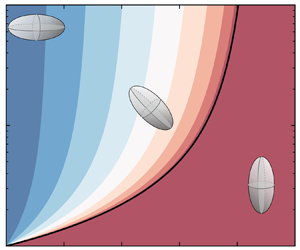
Figure 5. Maximum eigenvalue of the Jacobian matrix of different terminal settling modes for (a–c) a prolate particle and (d–f) an oblate particle. The aspect ratio and mass centre offset vary, while the density ratio and Galileo number are fixed at  $\alpha =3$ and $Ga=4$. (a,d) Top-heavy settling mode, (b,e) bottom-heavy settling mode, (c,f) oblique settling mode. The black solid line represents the critical mass centre offset $\bar {d}_{cr}$. The grey zone in panel (c,f) represents the parameter space where $\bar {d}>\bar {d}_{cr}$ and the oblique settling mode does not exist. The spheroid in each panel depicts the schematic of each settling mode.
Furthermore, we illustrate the pitch angle and drift angle of the spheroid in the steady settling mode (denoted by the subscript ‘ $s$’) in figure 6. First, when the mass centre coincides with the geometric centre (i.e. $\bar {d}=0$), the steady pitch angle is $\theta _s=90^\circ$ for a prolate particle or $\theta _s=0^\circ$ for an oblate particle, which is actually the value of $\theta _3$ with $\bar {d}=0$. In fact, this is a special case of the oblique settling mode, i.e. a broad-side-on alignment of the settling spheroid with a zero horizontal drift ( $\psi _s=0$). This stable alignment is the result of the fluid-inertia torque acting on the settling spheroid with a symmetric mass distribution (Dabade et al. Reference Dabade, Marath and Subramanian2015). Second, when $\bar {d}$ is greater than $\bar {d}_{cr}$, the bottom-heavy settling mode becomes stable and the spheroid settles with a narrow-side-on alignment, which also results in a zero horizontal drift. Third, when the mass centre offset is set between $0$ and $d_{cr}$, the spheroid settles in an oblique alignment. As indicated by the arrow in figure 6(a,c), the steady pitch angle ( $\theta _s$) progressively increases from $90^\circ$ to $180^\circ$ for a prolate particle (or from $0^\circ$ to $90^\circ$ for an oblate particle) as $\bar {d}$ increases from $0$ to $\bar {d}_{cr}$, corresponding to a transition of particle orientation from the broad-side-on to the narrow-side-on alignment. Throughout this transition, the settling velocity increases monotonously according to (4.4). However, the drift angle $\psi _s$ exhibits a non-monotonous variation with a local maximum for an intermediate oblique orientation. As depicted in figure 6(b,d), the maximum value of the drift angle increases as the particle asphericity grows. More detailed discussions regarding the maximum drift angle are provided in § 4.3.

Figure 6. Variation of (a,d) the steady pitch angle and (b,e) the steady drift angle of the settling spheroid with the change of aspect ratio and mass centre offset. The density ratio and Galileo number are fixed at  $\alpha =3$ and $Ga=4$. (c,f) The schematic diagrams of the steady pitch angle $\theta _s$ and the steady drift angle $\psi _s$. (a–c) Prolate particles, (c,d) oblate particles. The black solid line in (a,b,d,e) represents the critical mass centre offset $\bar {d}_{cr}$.
Next, we move on to examining the effect of density ratio and Galileo number on the stability of different settling modes. To do so, we vary the values of  $\alpha$ and $Ga$ and fix the aspect ratio $\lambda$ and the mass centre offset $\bar {d}$. As shown in figure 7, the top-heavy settling mode remains unconditionally unstable; the oblique settling mode is stable as long as it exists when $\bar {d}<\bar {d}_{cr}$; and the bottom-heavy settling mode becomes stable when $\bar {d}$ is greater than $\bar {d}_{cr}$. We note that the stability of each settling mode exhibited here is qualitatively the same as what is shown in figure 5 with varying $\lambda$ and $\bar {d}$ and fixed $\alpha$ and $Ga$.
$Ga$.

Figure 7. Same as figure 5 but for varying  $\alpha$ and $Ga$ with the mass centre offset fixed at $\bar {d}=0.005$ and the aspect ratio fixed at (a–c) $\lambda =2$ (prolate particle) or (d–f) $\lambda =0.5$ (oblate particle).
Moreover, similar to figure 6, we illustrate the steady pitch angle and drift angle of the settling spheroid with varying  $\alpha$ and $Ga$ but fixed $\bar {d}$ and $\lambda$ in figure 8. Here, the transition from the oblique settling mode to the bottom-heavy settling mode as $\alpha$ or $Ga$ decreases is ascribed to the decrease of $\bar {d}_{cr}$ (as indicated by the arrow in figure 8a,c). Throughout this transition, the drift angle $\psi _s$ also exhibits a non-monotonous variation (figure 8b,d), similar to the results shown in figure 6(b,e).

Figure 8. Variation of (a,c) the steady pitch angle and (b,d) the steady drift angle of the settling spheroid with the change of Galileo number and density ratio. The mass centre offset is fixed at  $\bar {d}=0.005$. (a,b) A prolate particle with $\lambda =2$, (c,d) an oblate particle with $\lambda =0.5$. The black line corresponds to $\bar {d}_{cr}=\bar {d}=0.005$.
4.2. Pitchfork bifurcation of particle settling motion
In the previous section we demonstrated the terminal settling motion of a spheroid shifts from the oblique mode to the bottom-heavy mode as  $\bar {d}$ increases from less than $\bar {d}_{cr}$ to greater than $\bar {d}_{cr}$. Here, we discuss the bifurcation characteristic through this transition. In figure 9 we present bifurcation diagrams of the steady settling mode of the spheroid with the variation of relevant parameters (i.e. $Ga$,
$Ga$,  $\alpha$, $\lambda$ and $\bar {d}$). There are two different sections of the steady pitch angle in each panel. On the one hand, the dual-branch structure of $\theta _s$ corresponds to the bi-steady oblique settling mode with $\theta =\theta _3$ or $\theta _4$. In this scenario, the preference of $\theta _3$ or $\theta _4$ as the terminal pitch angle for the settling spheroid is determined by the initial releasing condition. On the other hand, the single-branch structure of $\theta _s$ corresponds to the bottom-heavy settling mode. According to figure 9, the transition from the bottom-heavy settling mode to the oblique settling mode exhibits a pitchfork bifurcation pattern, which is the same as the bifurcation behaviour of a settling rod with mass eccentricity in the experiments of Roy et al. (Reference Roy, Hamati, Tierney, Koch and Voth2019). In principle, this pitchfork bifurcation can be induced in two ways: by changing $\bar {d}$ with a certain $\bar {d}_{cr}$ (figure 9d,h), or by varying $\bar {d}_{cr}$ through tuning the involved parameters ( $Ga$,
$Ga$,  $\alpha$ or $\lambda$) with a fixed $\bar {d}$ (figures 9a–c and 9e–g).

Figure 9. Bifurcation diagrams of the steady pitch angle  $\theta _s$ with the variation of (a,e) $Ga$, (b,f) $\alpha$, (c,g) $\lambda$ or (d,h) $\bar {d}$. The other three influencing parameters are fixed as indicated in each panel. (a–d) Prolate particles, (e–h) oblate particles.
Last but not least, we can infer from figure 9(d,h) that the spheroid is able to favour an oblique pitch angle between the broad-side-on to narrow-side-on alignment by the adjustment of  $\bar {d}$. This finding enlightens us on the possibility of manipulating the settling motion of spheroidal particles by adjusting their mass centre position.
4.3. Horizontal drift
In this section we further explore the horizontal drift of the settling spheroid. According to the formulation of the drift angle  $\psi$ (4.6), we can derive the maximum drift angle $\psi _{max}$ over all pitch angle as
 \begin{equation} {\psi _{max }} = \arctan \left( {\frac{{| {\kappa - 1} |}}{{2\sqrt \kappa }}} \right). \end{equation}
Here,  $\kappa =X^A/Y^A$ is a shape-dependent parameter. Recalling the characteristic settling velocities $v_1$ and $v_3$ as defined in (3.13), we find that $\kappa$ can be physically interpreted as the ratio between $v_1$ and $v_3$:
 \begin{equation} \kappa = \frac{{{v_1}}}{{{v_3}}} = \frac{{{X^A}}}{{{Y^A}}}.\end{equation}
Accordingly,  $\kappa$ is referred to as the velocity ratio that measures the range of variation of the settling velocity ( $v_{sett}$) of a spheroid. As shown in figure 10(a), with the increase of $\lambda$, the velocity ratio decreases monotonously from a value greater than one ( $\lambda <1$) to less than unity ( $\lambda >1$). This finding indicates that the range of variation in settling velocity increases as the particle shape deviates further from a sphere. For an infinitely thin disk ( $\lambda \rightarrow 0$) or an infinitely elongated rod ( $\lambda \rightarrow \infty$), the values of the velocity ratio $\kappa$ are
 \begin{gather} \mathop {\lim }_{\lambda \to 0} \kappa = 1.5, \end{gather}
 \begin{gather}\mathop {\lim }_{\lambda \to \infty } \kappa = 0.5. \end{gather}
Regarding the maximum drift angle  $\psi _{max}$, it is a function of $\kappa$ according to (4.10). Thus, $\psi _{max}$ is also solely determined by the aspect ratio. As shown in figure 10(b), $\psi _{max}$ increases as the degree of particle asphericity increases. In other words, more elongated prolate particles or thinner oblate particles are capable of experiencing greater horizontal drift by adjusting their mass centre offset. Furthermore, by substituting (4.12) and (4.13) into (4.10), we can obtain the maximum drift angle for an infinitely elongated rod and an infinitely thin disk as
 \begin{gather} \mathop{\max}_{\lambda > 1} \{ {{\psi _{max}}} \} = \mathop{\lim }_{\lambda \to \infty } {\psi _{max}} = \arctan \left( {\frac{{\sqrt 2 }}{4}} \right)\ {\rm rad} \approx 19.5^\circ, \end{gather}
 \begin{gather}\mathop{\max }_{\lambda < 1} \{ {{\psi _{max}}} \} = \mathop{\lim }_{\lambda \to 0} {\psi _{max}} = \arctan \left( {\frac{{\sqrt 6 }}{{12}}} \right)\ {\rm rad} \approx 11.5^\circ. \end{gather}
Figure 10. Dependence of (a) the velocity ratio  $\kappa$ and (b) the maximum drift angle $\psi _{max}$ on the aspect ratio of the spheroid.
5. Results: gravitational collision of settling spheroidal particles
In § 4 we have demonstrated that adjusting the mass centre position can change the terminal settling orientation of a spheroidal particle. Based on this finding, we investigate the collision kernel of settling spheroidal particles with different orientations in this section, to study how mass eccentricity influences the gravitational collision rate. In the following, we consider two different orientation distributions of dispersed particles: a completely random orientation and a partially random orientation with a fixed pitch angle. To examine the gravitational collision rate, we will first derive the approximate kinematic collision kernel, and then conduct Monte Carlo simulations to compute the dynamic collision kernel in these two scenarios.
5.1. Approximate kinematic collision kernel
According to the theory introduced in § 3.2.2, the primary focus should be fixed on the calculation of RRV to obtain the kinematic collision kernel of dispersed particles.
5.1.1. Random orientation
The problem of geometric collision of settling spheroidal particles with random orientations was proposed by Siewert et al. (Reference Siewert, Kunnen and Schröder2014). Without the consideration of mass eccentricity and fluid-inertia torque, settling spheroidal particles do not experience any change in their orientation after being released. Consequently, the orientation distribution of dispersed particles is assumed to be completely random. Under this assumption, the mean RRV ( $\langle |W_r |\rangle$) can be derived as follows (Siewert et al. Reference Siewert, Kunnen and Schröder2014):
 \begin{align} &\langle|W_{r}(R_{12})|
\rangle=\frac{1}{2{\rm \pi}
R_{12}^{2}}\int_{0}^{2{\rm \pi}}\int_{0}^{{\rm \pi}/2}
|(\boldsymbol{v}_{1}-\boldsymbol{v}_{2})\boldsymbol{\cdot}
\frac{\boldsymbol{x}_{1}-\boldsymbol{x}_{2}}{\|\boldsymbol{x}_{1}-
\boldsymbol{x}_{2}\|}|R_{12}\sin\theta_{c}\,
\mathrm{d}\theta_{c}R_{12} \,\mathrm{d}\phi_{c} \nonumber\\
&\quad =\frac{1}{32{\rm \pi}^3R_{12}^2}\tau_p g
c(\lambda)\int_0^{2{\rm \pi}}\int_0^{{\rm \pi}/{2}}
\int_0^{2{\rm \pi}}\int_{-{\rm \pi}/{2}}^{{\rm \pi}/{2}}
\int_0^{2{\rm \pi}}\int_{-{\rm \pi}/{2}}^{{\rm \pi}/{2}}\nonumber\\ &
\qquad\times R_{12}^2\sin\theta_c
\left|\begin{pmatrix}(\cos\theta_1\sin\theta_1\sin\phi_1-
\cos\theta_2\sin\theta_2\sin\phi_2)\sin\theta_c\cos\phi_c\\
+(-\cos\theta_1\sin\theta_1\cos\phi_1 + \cos\theta_2\sin\theta_2\cos\phi_2)
\sin\theta_c\sin\phi_c\\
+(\cos^2\theta_1-\cos^2\theta_2)\cos\theta_c\end{pmatrix}
\sin\theta_1\sin\theta_2\right|\nonumber\\ & \qquad
\times\mathrm{d}\theta_1 \,\mathrm{d}\phi_1 \,\mathrm{d}\theta_2
\,\mathrm{d}\phi_2 \,\mathrm{d}\theta_c \,\mathrm{d}\phi_c
=\frac{{\rm \pi}^{2}}{32}\tau_{p}g c(\lambda).
\end{align}
\begin{align} &\langle|W_{r}(R_{12})|
\rangle=\frac{1}{2{\rm \pi}
R_{12}^{2}}\int_{0}^{2{\rm \pi}}\int_{0}^{{\rm \pi}/2}
|(\boldsymbol{v}_{1}-\boldsymbol{v}_{2})\boldsymbol{\cdot}
\frac{\boldsymbol{x}_{1}-\boldsymbol{x}_{2}}{\|\boldsymbol{x}_{1}-
\boldsymbol{x}_{2}\|}|R_{12}\sin\theta_{c}\,
\mathrm{d}\theta_{c}R_{12} \,\mathrm{d}\phi_{c} \nonumber\\
&\quad =\frac{1}{32{\rm \pi}^3R_{12}^2}\tau_p g
c(\lambda)\int_0^{2{\rm \pi}}\int_0^{{\rm \pi}/{2}}
\int_0^{2{\rm \pi}}\int_{-{\rm \pi}/{2}}^{{\rm \pi}/{2}}
\int_0^{2{\rm \pi}}\int_{-{\rm \pi}/{2}}^{{\rm \pi}/{2}}\nonumber\\ &
\qquad\times R_{12}^2\sin\theta_c
\left|\begin{pmatrix}(\cos\theta_1\sin\theta_1\sin\phi_1-
\cos\theta_2\sin\theta_2\sin\phi_2)\sin\theta_c\cos\phi_c\\
+(-\cos\theta_1\sin\theta_1\cos\phi_1 + \cos\theta_2\sin\theta_2\cos\phi_2)
\sin\theta_c\sin\phi_c\\
+(\cos^2\theta_1-\cos^2\theta_2)\cos\theta_c\end{pmatrix}
\sin\theta_1\sin\theta_2\right|\nonumber\\ & \qquad
\times\mathrm{d}\theta_1 \,\mathrm{d}\phi_1 \,\mathrm{d}\theta_2
\,\mathrm{d}\phi_2 \,\mathrm{d}\theta_c \,\mathrm{d}\phi_c
=\frac{{\rm \pi}^{2}}{32}\tau_{p}g c(\lambda).
\end{align}
Here,  $\boldsymbol {x}_1$ and $\boldsymbol {x}_2$ represent the positions of two particles with a centre-to-centre distance of the collision radius $R_{12}$. The six-fold integral in (5.1) represents the average over all possible orientations of particles and all relative directions of pairwise particles. Moreover, $c(\lambda )$ is a dimensionless shape-dependent function defined by
 \begin{equation} c(\lambda)=\left|\frac1{X^A}-\frac1{Y^A}\right|\frac{r_e}a, \end{equation}
which is plotted in figure 11. Substituting the expression of  $\langle |W_r |\rangle$ into (3.32), and regarding $D_{eq}$ as the collision radius, we can obtain the approximate kinematic collision kernel as
 \begin{equation} \varGamma^K_{rand}=\frac{{\rm \pi}^3}{16} D_{eq}^2 \tau_p g c(\lambda). \end{equation}
Here, the subscript ‘rand’ denotes the completely random distribution of particle orientations. Indicated by (5.3), the collision kernel is proportional to the shape-dependent function  $c(\lambda )$, which implies a vanishing $\varGamma _{rand}^K$ for spherical particles since $c(\lambda )$ is equal to zero at $\lambda =1$. This makes sense as spherical particles with an equal size settle with the same velocity and have no chance to collide. In the following parts, we regard $\varGamma _{rand}^K$ as a characteristic collision kernel to normalize the collision kernel in other cases.

Figure 11. Plot of the shape-dependent function  $c(\lambda )$ versus the aspect ratio $\lambda$.
5.1.2. Fixed pitch angle
As discussed in § 4, the terminal settling state of a spheroidal particle depends on its mass centre offset when the fluid-inertia torque is involved. By adjusting  $\bar {d}$, the spheroid can settle with an arbitrary pitch angle between the broad-side-on and narrow-side-on alignment. Therefore, we consider a partially random distribution of particle orientations: a random distribution of the azimuth angle $\phi$ but a fixed pitch angle with $\theta =\theta _0$. By varying $\theta _0$, we can investigate how the change of mass centre offset affects the gravitational collision rate. In view of the symmetry, we restrict our discussion on the fixed pitch angle ranging from $\theta _0=0^\circ$ to $\theta _0=90^\circ$, which encompasses all possible orientations from the broad-side-on to narrow-side-on alignment for settling spheroidal particles.
In this scenario, the calculation of ( $\langle |W_r |\rangle$ is achieved by averaging over all possible azimuth angles $\phi$ and relative directions of particle pairs as follows:
 \begin{align} &\langle|W_{r}(R_{12})|
\rangle=\frac{1}{2{\rm \pi}
R_{12}^{2}}\int_{0}^{2{\rm \pi}}\int_{0}^{{\rm \pi}/2}
\left|(\boldsymbol{v}_{1}-\boldsymbol{v}_{2})\boldsymbol{\cdot}
\frac{\boldsymbol{x}_{1}-\boldsymbol{x}_{2}}{\|\boldsymbol{x}_{1}-
\boldsymbol{x}_{2}\|}\right|R_{12}\sin\theta_{c}\,
\mathrm{d}\theta_{c}R_{12} \,\mathrm{d}\phi_{c} \nonumber\\
&\quad =\frac{1}{8{\rm \pi}^3R_{12}^2}\tau_p g
c(\lambda)\int_0^{2{\rm \pi}}\int_0^{{\rm \pi}/{2}}\int_0^{2{\rm \pi}}\int_0^{2{\rm \pi}}\nonumber\\
& \qquad\times \left| \begin{array}{c} \cos {\theta _0}\sin
{\theta _0}( {\sin {\phi _1} - \sin {\phi _2}} )\sin
{\theta _c}\cos {\phi _c} \hfill \\ - \cos {\theta _0}\sin
{\theta _0}( {\cos {\phi _1} - \cos {\phi _2}} )\sin
{\theta _c}\sin {\phi _c} \hfill \\ \end{array}\right|
\mathrm{d}\phi_1 \,\mathrm{d}\phi_2 \,\mathrm{d}\theta_c
\,\mathrm{d}\phi_c \nonumber\\ &\quad =\frac{1}{\rm \pi} |
\sin (2\theta_0)|\tau_{p}g c(\lambda).
\end{align}
\begin{align} &\langle|W_{r}(R_{12})|
\rangle=\frac{1}{2{\rm \pi}
R_{12}^{2}}\int_{0}^{2{\rm \pi}}\int_{0}^{{\rm \pi}/2}
\left|(\boldsymbol{v}_{1}-\boldsymbol{v}_{2})\boldsymbol{\cdot}
\frac{\boldsymbol{x}_{1}-\boldsymbol{x}_{2}}{\|\boldsymbol{x}_{1}-
\boldsymbol{x}_{2}\|}\right|R_{12}\sin\theta_{c}\,
\mathrm{d}\theta_{c}R_{12} \,\mathrm{d}\phi_{c} \nonumber\\
&\quad =\frac{1}{8{\rm \pi}^3R_{12}^2}\tau_p g
c(\lambda)\int_0^{2{\rm \pi}}\int_0^{{\rm \pi}/{2}}\int_0^{2{\rm \pi}}\int_0^{2{\rm \pi}}\nonumber\\
& \qquad\times \left| \begin{array}{c} \cos {\theta _0}\sin
{\theta _0}( {\sin {\phi _1} - \sin {\phi _2}} )\sin
{\theta _c}\cos {\phi _c} \hfill \\ - \cos {\theta _0}\sin
{\theta _0}( {\cos {\phi _1} - \cos {\phi _2}} )\sin
{\theta _c}\sin {\phi _c} \hfill \\ \end{array}\right|
\mathrm{d}\phi_1 \,\mathrm{d}\phi_2 \,\mathrm{d}\theta_c
\,\mathrm{d}\phi_c \nonumber\\ &\quad =\frac{1}{\rm \pi} |
\sin (2\theta_0)|\tau_{p}g c(\lambda).
\end{align}
Since the pitch angle of the particle is fixed at  $\theta _1=\theta _2=\theta _0$, the average is reduced to a four-fold integral instead of the six-fold integral in (5.1). Accordingly, the approximate kinematic collision kernel can be written as
 \begin{equation} \varGamma_{fix}^K=\varGamma_{fix}^K(\theta_0)= 2|\sin(2\theta_0)|D_{eq}^2\tau_pg c(\lambda). \end{equation}
The subscript ‘fix’ indicates the fixed pitch angle of dispersed particles. Same as  $\varGamma _{rand}^K$, $\varGamma _{fix}^K$ is also proportional to the shape-dependent function $c(\lambda )$. Thus, the ratio $\varGamma _{fix}^K/\varGamma _{rand}^K$ is independent of particle shape, but is correlated with the pitch angle by the function of $|\sin (2\theta _0)|$, as illustrated in figure 12. The maximum value of $\varGamma _{fix}^K/\varGamma _{rand}^K$ is $32/{\rm \pi} ^3\approx 1.03$ at $\theta _0=45^\circ$.

Figure 12. Plot of  $\varGamma _{fix}^K$ normalized by $\varGamma _{rand}^K$ with the variation of $\theta _0$.
Interestingly, as discussed in § 4.1, the horizontal drift velocity of a settling spheroidal particle is also correlated with the pitch angle by  $|\sin (2\theta )|$ (see (4.5)), just as $\varGamma _{fix}^K$ does. The relationship between the collision kernel and the drift velocity can be interpreted as follows. According to (4.4), dispersed particles with a fixed pitch angle settle with the same vertical velocity. Thus, the geometric collision can only be caused by the difference of their horizontal drift velocities. Therefore, it is rational that the correlation of particle drift velocity with the pitch angle is the same as that of the gravitational collision kernel. Especially, as for the narrow-side-on or broad-side-on settling ( $\theta _0=0^\circ$ or $90^\circ$), the collision kernel $\varGamma _{fix}^K$ vanishes since the particles experience zero horizontal drift with these two orientations.
5.2. Dynamic collision kernel
In the derivation of the approximate kinematic collision kernel for spheroidal particles, we introduce an assumption that the collision radius is equal to the particle equivalent diameter (Siewert et al. Reference Siewert, Kunnen and Schröder2014). However, this assumption needs to be further examined. Hence, we conduct Monte Carlo simulations of settling spheroidal particles to determine the dynamic collision kernel  $\varGamma ^D$. The configuration of the Monte Carlo simulation is provided in table 1.
Table 1. Dimensionless parameters for the Monte Carlo simulation of settling spheroidal particles. For the normalization, we choose the particle equivalent diameter  $D_{eq}$ as the characteristic length scale, $\tau _p g c(\lambda )$ as the characteristic velocity and $D_{eq}/(\tau _p g c(\lambda ))$ as the characteristic time scale. Here $\phi$ represents the particle volume fraction.
5.2.1. Random orientation
We first consider settling spheroidal particles with random orientations. We choose eight particle shapes: oblate particles with aspect ratio  $\lambda =0.2, 0.33, 0.5, 0.8$ and prolate particles with aspect ratio $\lambda =1.2, 2, 3, 5$. Figure 13(a) illustrates the dynamic collision kernels obtained by the Monte Carlo simulation. It can be inferred that the approximate kinematic collision kernel underestimates the dynamic collision kernel for most particle shapes (except for a slight overestimation for the case of $\lambda =1.2$). The difference between $\varGamma _{rand}^D$ and $\varGamma _{rand}^K$ becomes more pronounced as the particle shape deviates further from a sphere, especially for oblate particles. This difference actually reflects the geometric complexity for the collision of spheroidal particles, which is ignored in deriving the approximate kinematic collision kernel. Nevertheless, in spite of the deviation, $\varGamma _{rand}^K$ still provides a reasonable estimation of the dynamic collision kernel, as long as the particle shape does not deviate significantly from a sphere. Even in the case of the greatest discrepancy here (the case of $\lambda =0.2$), $\varGamma _{rand}^K$ is still within the same order of magnitude as $\varGamma _{rand}^D$.

Figure 13. Normalized dynamic collision kernel of settling spheroidal particles obtained by the Monte Carlo simulation. (a) Random orientation. (b) Fixed pitch angle. The approximate kinematic collision kernel  $\varGamma _{fix}^K$ (indicated by ‘kinematic’ in the legend) is included for comparison.
5.2.2. Fixed pitch angle
Then we move on to the case of settling spheroidal particles with a fixed pitch angle. Figure 13(b) shows the comparison of the dynamic collision kernel obtained by the Monte Carlo simulation and the approximate kinematic collision kernel for spheroidal particles with different aspect ratios and different pitch angles. The difference between  $\varGamma _{fix}^D$ and $\varGamma _{fix}^K$ is manifested in two aspects. Firstly, $\varGamma _{fix}^D$ exhibits a skewed dependence on $\theta _0$ towards the narrow-side-on alignment side ( $\theta _0=0^\circ$ side for oblate particles and $\theta _0=90^\circ$ side for prolate particles), which is different from the symmetry function of $\varGamma _{fix}^K(\theta _0)$ about $\theta _0=45^\circ$. Secondly, the normalized dynamic collision kernel ( $\varGamma _{fix}^D/\varGamma _{rand}^K$) is not only a function of the pitch angle but also dependent on particle aspect ratio. The discrepancy between $\varGamma _{fix}^K$ and $\varGamma _{fix}^D$, which is generally manifested by an underestimation of the exact collision rate by $\varGamma _{fix}^K$, becomes more pronounced with the increase of particle asphericity. Nevertheless, in spite of these differences, we demonstrate that $\varGamma _{fix}^K$ qualitatively captures the non-monotonic variation trend of the dynamic collision kernel with the change of $\theta _0$.
In summary, by conducting Monte Carlo simulations, we verified the results obtained in § 5.1 that the collision rate of settling spheroidal particles reaches its maximum when particles settle with an intermediate pitch angle. This finding enlightens us to manipulate the gravitational collision rate of settling spheroidal particles by adjusting the mass centre position.
6. Discussion and conclusions
6.1. Discussion: extend to turbulent flows
Although the present study is conducted by only considering the simplest quiescent fluid as the background flow, the results are relevant in the case of turbulent flows. Here, we provide a discussion on the collision of particles with mass centre offset in turbulent flows. In the previous studies on the settling particles in turbulence, Siewert et al. (Reference Siewert, Kunnen and Schröder2014) and Jucha et al. (Reference Jucha, Naso, Lévêque and Pumir2018) have demonstrated that the collision rate of non-spherical particles is enhanced compared with spherical ones, since the settling spheroidal particles with random orientations increases the RRV. This conclusion was drawn without considering the fluid-inertia torque and gravitational torque induced by mass centre offset. To analyse the collision rate of settling spheroidal particles in turbulent flows with the inclusion of these two torques, the orientation of particles has to be re-examined.
In general, there are three torques determining the orientation of particles in turbulent flows. The first is the shear-induced torque, i.e. Jeffery torque, which can be estimated by  $T_J \sim \mu a^3 |\boldsymbol {\omega }-\boldsymbol {\varOmega }|$. While the vorticity fluctuations in the turbulent flow randomize the orientation of dispersed particles. The second one is the fluid-inertia torque, which can be estimated by $T_I \sim \rho _f a^3 |\boldsymbol {u}-\boldsymbol {v}|^2$. Under the action of this torque, spheroidal particles tend to settle with broad-side-on. The third is the gravitational torque related to the mass centre offset, which can be estimated by $T_g \sim \rho _p V_p g d$. As discussed in the present work, this torque aligns the major axis of the settling spheroids in the gravitational direction.
In the earlier study, Anand, Ray & Subramanian (Reference Anand, Ray and Subramanian2020) explored the effect of fluid inertia on the orientation of settling spheroids in turbulence and found that the fluid-inertia torque leads to the broad-side-on alignment. Furthermore, Sheikh et al. (Reference Sheikh, Gustavsson, Lopez, Lévêque, Mehlig, Pumir and Naso2020) discussed the competition between the fluid-inertia torque and Jeffery torque by defining a dimensionless parameter  $R=|\boldsymbol {u}-\boldsymbol {v}|^2/(\nu |\boldsymbol {\omega }-\boldsymbol {\varOmega }|)$. They demonstrated that spheroidal particles tend to settle with the broad-side-on alignment when the fluid-inertia effect is dominant with $R \gg 1$. While, in a strong turbulent flow where $R \ll 1$, the turbulent shear effect prevails, leading to a random orientation distribution of dispersed particles. If we further introduce the effect of mass centre offset into this problem, the relative strength of $T_I$, $T_J$ and $T_g$ should be examined. It can be predicted that if the mass centre offset is large enough to make the gravitational torque overwhelm the other two torques, the narrow-side-on alignment would be present. Moreover, if the gravitational torque is comparable to the fluid-inertia torque, and both of them are much stronger than the Jeffery torque, settling spheroidal particles would preferentially favour an oblique orientation, which is determined by the specific ratio between $T_I$ and $T_g$ as discussed in the present work.
The enhanced collision rate of spheroidal particles with random orientations reported in Siewert et al. (Reference Siewert, Kunnen and Schröder2014) and Jucha et al. (Reference Jucha, Naso, Lévêque and Pumir2018) occurs when  $T_J$ plays a predominant role. However, if the fluid-inertia torque or the gravitational torque dominates, the RRV induced by settling velocity would be considerably attenuated since particles prefer the broad-side-on or narrow-side-on alignment (corresponding to the case of a fixed pitch angle $\theta _0=0$ or $\theta _0={\rm \pi} /2$). While, in the scenario where $T_I$ is comparable with $T_g$ but much greater than $T_J$, the RRV of colliding particles could be primarily predicted by the situation of a fixed pitch angle, which has been discussed in §§ 5.1.2 and 5.2.2.
Nevertheless, the above qualitative discussion only considers the contribution of settling-velocity-induced RRV to the collision rate of spheroidal particles in turbulent flows. However, as for settling inertial particles in turbulent flows, the collision rate would also be affected by other effects, such as the sling effect (Falkovich & Pumir Reference Falkovich and Pumir2007; Jucha et al. Reference Jucha, Naso, Lévêque and Pumir2018), preferential concentration at low-vorticity regions (Sundaram & Collins Reference Sundaram and Collins1997; Zhou, Wexler & Wang Reference Zhou, Wexler and Wang1998; Pumir & Wilkinson Reference Pumir and Wilkinson2016; Anand et al. Reference Anand, Ray and Subramanian2020) and preferential sweeping effect to enhance settling velocity (Ghosh et al. Reference Ghosh, Dávila, Hunt, Srdic, Fernando and Jonas2005; Good et al. Reference Good, Ireland, Bewley, Bodenschatz, Collins and Warhaft2014; Anand et al. Reference Anand, Ray and Subramanian2020). A quantitative study on the effects of fluid-inertia torque and mass centre offset on particle behaviour in turbulence is left for future work.
6.2. Conclusions and prospect for future work
In this study we have investigated the effect of mass centre offset on the settling motion and gravitational collision rate of spheroidal particles in a quiescent fluid under the low-Reynolds-number assumption.
We firstly analysed the settling motion of a single spheroid with an offset mass centre. Based on the Newton–Euler equations, we derived a critical mass centre offset that determines the terminal settling mode of the spheroid. When the mass centre coincides with the geometric centre, a spheroid settles with the broad-side-on alignment under the action of the fluid-inertia torque. With a non-zero mass centre offset below the critical threshold, a spheroid prefers an oblique settling mode, in which the fluid-inertia torque balances with the gravitational torque. The spheroid drifts horizontally in this mode, due to the misalignment of its velocity and the direction of gravity. However, when the mass centre offset exceeds the critical value, the gravitational torque is dominant, and the spheroid settles in a bottom-heavy mode with a narrow-side-on alignment and vanishing horizontal drift. Therefore, we conclude that the orientation of a settling spheroid undergoes a transition from the broad-side-on to narrow-side-on alignment as the mass centre offset increases from zero to the critical value. This transition, which is found to follow a pitchfork bifurcation pattern, can be induced either by the change of mass centre offset, or by varying the critical mass centre offset through tuning the density ratio, Galileo number or aspect ratio. Moreover, we further analysed the horizontal drift of the spheroid. The maximum drift angle is found to be a function of velocity ratio between narrow-side-on and broad-side-on settling. As the shape of the spheroid deviates further from a sphere, both the velocity ratio and the maximum drift angle increase accordingly.
In the second part of this work, we shifted to study the gravitational collision rate of settling spheroidal particles with different orientations. First, we originally derived the approximate kinematic collision kernel of settling spheroidal particles with a fixed pitch angle, following the theoretical model proposed by Siewert et al. (Reference Siewert, Kunnen and Schröder2014). It is found that the approximate kinematic collision correlates with the pitch angle in the same manner as the drift velocity does. Then, Monte Carlo simulations are conducted to determine the dynamic collision kernel of settling particles. It is demonstrated that the collision kernel of settling spheroidal particles varies from zero (for the broad-side-on or narrow-side-on alignment) to a maximum value (for an intermediate oblique orientation) with the change of pitch angle. Furthermore, the comparison between the kinematic and dynamic collision kernel reveal that the approximate kinematic collision kernel of spheroidal particles underestimates the collision rate in most scenarios. This discrepancy is related to the geometric complexity for colliding spheroids and becomes more significant with the increase of particle asphericity. However, despite the discrepancy, the approximate kinematic collision kernel is qualitatively correct and provides a reasonable estimation of the dynamic collision kernel for spheroidal particles, as long as the particle does not deviate significantly from a spherical shape. This finding justifies the rationality of the theory of approximate kinematic collision kernel for spheroidal particles as provided in § 3.2.2. By expressing the collision kernel in a kinematic manner, the collision rate of particles can be estimated based on the collective statistics of dispersed particles, rather than relying on complicated procedures of collision detection and counting. This is particularly helpful in establishing theoretical models for collision rates of non-spherical particles in other complex scenarios, such as turbulent particle-laden flows.
According to our analysis, the settling motion of a spheroidal particle is highly sensitive to the mass centre offset. For example, according to (4.8), as for a prolate particle with an aspect ratio  $\lambda =3$, density ratio $\alpha =2$ and Galileo number $Ga=4$, the value of $\bar {d}_{cr}$ is only $0.0734$. This indicates that even a small degree of the offset between particle mass centre and its geometric centre can result in a substantial change of particle alignment from broad-side-on to narrow-side-on. Regarding the collision in a multi-particle system, it also reveals a sensitive dependency of collision rate on the mass centre offset. These findings highlight the importance of considering mass eccentricity in practical applications involving settling non-spherical particles, even in the cases where the extent of deviation between particle mass centre and geometric centre is small. Furthermore, the present results also imply the possibility for the manipulation of the settling motion and collision rate of spheroidal particles by adjusting their mass centre position.
Finally, we discuss the potential valuable work awaiting future explorations as follows. First, with the focus on the terminal settling state of the spheroid, we restrict the mass centre on the symmetry-vertical plane in the present study. However, when the mass centre is not located on the symmetry axis of the spheroid and deviates from the symmetry-vertical plane, our preliminary exploration in Appendix C demonstrates that the spinning (rotation around the symmetry axis) and tumbling (rotation around the axis perpendicular to the symmetry axis) motions of the spheroid are coupled in the developing stage. The three-dimensional angular dynamics in this scenario may introduce more intricate bifurcation behaviour of the rotation of the spheroid. What and how the relevant factors influence the developing process for the three-dimensional rotation are unknown and remain for further investigation. Second, we propose a way to manipulate the orientation of non-spherical particles in the present work. Although we only consider the quiescent flow, this mechanism should also play a significant role in turbulent flows. As discussed in § 6.1, the coupled effect of turbulent shear, fluid-inertia torque and mass centre offset may result in an intricate behaviour of the orientations and collisions of non-spherical particles in turbulent flows, which can be explored in the future. Third, it is important to note that all the results presented in this study are obtained within the low-Reynolds-number limit with a disregard of particle–particle hydrodynamic interactions. In future work these limits can be broken by performing particle-resolved direct numerical simulations of settling spheroidal particles with an offset mass centre.
Funding
This work is supported by the Natural Science Foundation of China (grant nos. 92252104, 12388101 and 92252204).
Declaration of interests
The authors report no conflict of interest.
Appendix A. Mass distribution of the particle
The mass centre position and moment of inertia of a spheroidal particle depend on the mass distribution. In this study we consider a spheroid with a hole located on its major axis (on the negative  $\hat {y}$ axis for a prolate particle or negative $\hat {x}$ axis for an oblate particle), as depicted in figure 14. To compensate the missing mass from the hole, an equivalent mass is added to the position that is mirror symmetric to the hole with respect to the equatorial plane ( $\hat {x}$– $\hat {z}$ plane) for a prolate particle or the meridional plane ( $\kern0.7pt \hat {y}$– $\hat {z}$ plane) for an oblate particle. This results in a heavy core located on the major axis with a density of $2\rho _p$, as indicated by the black region in figure 14. In this manner, the mass centre of the spheroid deviates from its geometric centre along the major axis.

Figure 14. Section views of the mass distribution inside (a) a prolate particle and (b) an oblate particle. The mass centre  $G$ of the spheroid deviates from its geometric centre $C$. Here $\boldsymbol {n}$ is the unit vector along the symmetry axis of the spheroid; $C\hat {x}\hat {y}\hat {z}$ is the body-fixed frame.
As for the spheroid with such a mass distribution, the moment of inertia about the geometric centre  $C$ is the same as that of a mass-uniform spheroid, i.e.
 \begin{equation} \hat{\boldsymbol{I}}_C=diag[I_{\hat{x}},I_{\hat{y}}, I_{\hat{z}}]=diag[\tfrac15m(r_{e}^{2}+r_{p}^{2}), \tfrac25mr_{e}^{2},\tfrac15m(r_{e}^{2}+r_{p}^{2})].\end{equation}
Therefore, according to the parallel-axis theorem of a rigid body, the moment of inertia of the spheroid about its mass centre  $G$ can be derived as
 \begin{align}
\hat{\boldsymbol{I}}_G(d)&=diag[I_{\hat{x}}-md^{2},I_{\hat{y}},
I_{\hat{z}}-md^{2}]\nonumber\\ &=diag[\tfrac{1}{5}m(a^{2}+b^{2}-5d^{2}),
\tfrac{2}{5}mb^{2},\tfrac{1}{5}m(a^{2}+b^{2}-5d^{2})]\end{align}
\begin{align}
\hat{\boldsymbol{I}}_G(d)&=diag[I_{\hat{x}}-md^{2},I_{\hat{y}},
I_{\hat{z}}-md^{2}]\nonumber\\ &=diag[\tfrac{1}{5}m(a^{2}+b^{2}-5d^{2}),
\tfrac{2}{5}mb^{2},\tfrac{1}{5}m(a^{2}+b^{2}-5d^{2})]\end{align}for a prolate particle and
 \begin{align}
\hat{\boldsymbol{I}}_G(d)&=diag[I_{\hat{x}},I_{\hat{y}}-md^{2},
I_{\hat{z}}-md^{2}]\nonumber\\ & =diag[ {\tfrac{1}{5}m({{a^2} + {b^2}} ),
\tfrac{1}{5}m( {2{a^2} - 5{d^2}} ),\tfrac{1}{5}m({{a^2} +
{b^2} - 5{d^2}} )} ]
\end{align}
\begin{align}
\hat{\boldsymbol{I}}_G(d)&=diag[I_{\hat{x}},I_{\hat{y}}-md^{2},
I_{\hat{z}}-md^{2}]\nonumber\\ & =diag[ {\tfrac{1}{5}m({{a^2} + {b^2}} ),
\tfrac{1}{5}m( {2{a^2} - 5{d^2}} ),\tfrac{1}{5}m({{a^2} +
{b^2} - 5{d^2}} )} ]
\end{align}
for an oblate particle. Consequently, the dimensional form of the radius of gyration  $r_I$ in (3.17) is
 \begin{equation} r_I=\sqrt{\frac{I_{\hat{z}}}m}=\sqrt{\frac{a^2+b^2-5d^2}5}.\end{equation}
 Note that in a limiting case where the hole is as large as half of the spheroid, all of the mass accumulates on half of the volume ( $\kern0.7pt \hat {y}>0$ half for a prolate particle or $\hat {x}>0$ half for an oblate particle). In this limiting case, the mass centre position of the spheroid is
 \begin{equation} \hat{\boldsymbol{x}}_G=\dfrac{\displaystyle \iiint_{\frac12V_p}2\rho_p \hat{\boldsymbol{x}}\,{\rm d}V}{\displaystyle \iiint_{V_p}\rho_p\,{\rm d}V}= \begin{cases}[0,0.375a,0]^T & (\lambda>1),\\ [0.375a,0,0]^T & (\lambda<1),\end{cases}\end{equation}
where  $V_p$ represents the whole volume of the spheroid and $\frac {1}{2} V_p$ represents the dense half-part. Therefore, the dimensionless mass centre offset $\bar {d}=d/a$ is constrained within the range of $\bar {d} \in [0,0.375]$.
Appendix B. Coefficients in the hydrodynamic forces and torques
The coefficients  $X^A$ and $Y^A$ presented in the Stokesian resistance tensor $\boldsymbol {M}_{st}$ in (3.5) are (Happel & Brenner Reference Happel and Brenner1983)
 \begin{gather} X^{A}=\left\{\begin{array}{ll} \displaystyle \dfrac{4 e^{3}}{3\left((2 e^{2}-1) \cot ^{{-}1}\left(\dfrac{\sqrt{1-e^{2}}}{e}\right) +e \sqrt{1-e^{2}}\right)} & (\lambda<1), \\ \displaystyle \dfrac{8 e^{3}}{3\left({-}2 e+(1+e^{2}) \ln \left(\dfrac{1+e}{1-e}\right)\right)} & (\lambda>1), \end{array}\right. \end{gather}
 \begin{gather}Y^{A}=\left\{\begin{array}{ll} \displaystyle \dfrac{8 e^{3}}{3\left(\left(2 e^{2}+1\right) \cot ^{{-}1}\left(\dfrac{\sqrt{1-e^{2}}}{e}\right)-e \sqrt{1-e^{2}}\right)} & (\lambda<1), \\ \displaystyle \dfrac{16 e^{3}}{3\left(2 e+\left({-}1+3 e^{2}\right) \ln \left(\dfrac{1+e}{1-e}\right)\right)} & (\lambda>1). \end{array}\right. \end{gather}
Here,  $e$ is the ellipticity of the spheroid defined by
 \begin{equation} e=\left\{\begin{array}{@{}ll} \sqrt{1-\lambda^2} & (\lambda<1), \\ \sqrt{1-(1/\lambda)^2} & (\lambda>1). \end{array}\right. \end{equation}
 The expressions of coefficients  $\alpha _0$ and $\beta _0$ involved in the Jeffery torque (3.6) are (Jeffery Reference Jeffery1922)
 \begin{gather} {{\alpha}}_{0} =\begin{cases} \dfrac{2}{1-\lambda^2}-\dfrac{2\arccos (\lambda)\lambda}{(1-\lambda^2)^{3/2}} & (\lambda<1), \\ \dfrac{-2}{\lambda^2-1}+\dfrac{2\text{arccosh} (\lambda)\lambda}{(\lambda^2-1)^{3/2}} & (\lambda>1),\end{cases} \end{gather}
 \begin{gather}\beta_0=\begin{cases} \displaystyle \frac{\lambda^2}{\lambda^2-1}+\frac{\arccos(\lambda) \lambda}{(1-\lambda^2)^{3/2}} & (\lambda<1), \\ \displaystyle \frac{\lambda^2}{\lambda^2-1}-\frac{\text{arccosh}(\lambda) \lambda}{(\lambda^2-1)^{3/2}} & (\lambda>1).\end{cases} \end{gather}
The coefficient  $h_\lambda$ presented in the expression of fluid-inertia torque (3.7) is (Dabade et al. Reference Dabade, Marath and Subramanian2015; Sheikh et al. Reference Sheikh, Gustavsson, Lopez, Lévêque, Mehlig, Pumir and Naso2020)
 \begin{align} h_\lambda &=\frac{{\rm \pi} e^3\sqrt{1-e^2}({-}420+3500e^2-9989e^4+4757e^6)}{315 \sqrt{1-e^2}({-}e\sqrt{1-e^2}+(1+2e^2)\sin^{{-}1}e) (e\sqrt{1-e^2}+(2e^2-1)\sin^{{-}1}e)^2} \nonumber\\ &\quad +\frac{210{\rm \pi} e^2(2-24e^2+69e^4-67e^6+20e^8) \sin^{{-}1}e}{315\sqrt{1-e^2}({-}e\sqrt{1-e^2}+(1+2e^2)\sin^{{-}1}e ) (e\sqrt{1-e^2}+(2e^2-1)\sin^{{-}1}e)^2} \nonumber\\ &\quad +\frac{105{\rm \pi} e^3(12-17e^2+24e^4) (\sin^{{-}1}e)^2}{315({-}e\sqrt{1-e^2}+(1+2e^2)\sin^{{-}1}e) (e\sqrt{1-e^2}+(2e^2-1)\sin^{{-}1}e)^2} \end{align}
for an oblate particle ( $\lambda <1$) and
 \begin{align} h_{\lambda}& =\frac{-{\rm \pi} e^{2} (420e+2240e^{3}+4249e^{5}-2152e^{7} )}{315 ( (e^{2}+1 )\tanh^{{-}1}e-e )^{2} ( (1-3e^{2} )\tanh^{{-}1}e-e )} \nonumber\\ &\quad +\frac{{\rm \pi} e^2 (420+3360e^2+1890e^4-1470e^6 )\tanh^{{-}1}e}{315 ( (e^2+1 )\tanh^{{-}1}e-e )^2 ( (1-3e^2 )\tanh^{{-}1}e-e )} \nonumber\\ &\quad -\frac{{\rm \pi} e^2 (1260e-1995e^3+2730e^5-1995e^7 ) (\tanh^{{-}1}e )^2}{315 ( (e^2+1 )\tanh^{{-}1}e-e )^2 ((1-3e^2 )\tanh^{{-}1}e-e )} \end{align}
for a prolate particle ( $\lambda >1$).
Appendix C. Three-dimensional rotation of the oblate spheroid
In this appendix we consider the three-dimensional rotation of an oblate spheroid with mass eccentricity settling in a quiescent fluid. As shown in figure 15, we define an azimuth angle  $\chi$ (which is different from the azimuth angle $\phi$ defined in figure 1) as the angle between the unit vector $\boldsymbol {p}$ and the symmetry-vertical plane.

Figure 15. Sketch of the three-dimensional rotation of an oblate spheroid with mass eccentricity. The unit vector along the direction from the centroid  $C$ to the mass centre $G$ is denoted by $\boldsymbol {p}$. The green plane represents the symmetry-vertical plane (the plane spanned by the direction along the symmetry axis ( $\boldsymbol {n}$) and the gravitational direction ( $\boldsymbol {e}_g$)).
To examine the three-dimensional rotation, we need to compute the six-degree-of- freedom motion of the spheroid by numerically solving the Newton–Euler equations (3.8)–(3.10). In figure 16 we provide a few examples of the solution of this problem. We consider an oblate spheroid with  $Ga=3,\alpha =3,\lambda =1/3$, while the mass centre offset and the initial condition are varied in different simulations. According to the results shown in figure 16(a–d), we observe that the mass centre always drifts to the symmetry-vertical plane (corresponding to $\chi =0$) in the terminal state, and the spheroid orientation converges to the steady pitch angle as provided in the main text, regardless of the value of $\bar {d}$ and the initial condition. Specifically, in the cases shown in figure 16(a,b,e,f), the narrow-side-on settling is finally reached ( $\theta _s=90^\circ$), since the mass centre offset is larger than the critical threshold (i.e. $\bar {d}>\bar {d}_{cr}$). In contrast, the oblique mode with a finite pitch angle ( $\theta _s \approx 47^\circ$) is preferred by the spheroid with $\bar {d}<\bar {d}_{cr}$ in the cases shown in figure 16(c,d,g,h). Therefore, the above results justify the two-dimensional simplification (setting $\chi =0$) adopted in the main text, if the terminal steady state of the spheroid is of concern.

Figure 16. Three-dimensional rotation of the oblate spheroid. (a–d) Time evolution of the pitch angle  $\theta$ and the azimuth angle $\chi$ ( $U_g =\sqrt {(\alpha -1)g D_{eq}}$ is the characteristic velocity used for the normalization of time); (e–h) phase diagram of the rotation on the $\theta -\chi$ plane. Mass centre offset varies in different panels: (a,e) $\bar {d}=0.1$, (b,f) $\bar {d}=0.05$, (e,g,d,h) $\bar {d}=0.02$. The initial condition is set as $\boldsymbol {n}_0=[-0.5,0.866,0]$ and $\boldsymbol {p}_0=[0.742,0.429,-0.515]$ (corresponding to $\theta _0=30^\circ$ and $\chi _0=15^\circ$) in the cases shown in (a–c, e–g), and $\boldsymbol {n}_0=[-0.866,0.5,0]$ and $\boldsymbol {p}_0=[0.235,0.407,-0.883]$ (corresponding to $\theta _0=60^\circ$ and $\chi _0=50^\circ$) in the case shown in (d,h). The dashed line in (a–d) represents the steady pitch angle $\theta _s$. The blue circle and red star in (e–h) represent the initial condition and the terminal state, respectively.
Additionally, note that the three-dimensional rotation can also appear for a prolate spheroid if the mass centre does not lie on the symmetry axis, although we only consider the case of an oblate spheroid as a preliminary exploration.
Appendix D. Low-Reynolds-number assumption
The expressions of Stokesian drag, Jeffery torque and fluid-inertia torque provided in (3.4)–(3.7) are only applicable under the low-Reynolds-number limit. Here, we define a maximum settling Reynolds number based on the maximum settling velocity of the spheroid as
 \begin{equation} Re_{_{p,max}}=\frac{\|\boldsymbol{v}_t\|_{{max}}D_{eq}}\nu= \frac{max\{v_1,v_3\}D_{eq}}\nu.\end{equation}
By substituting the expressions of  $v_1$ and $v_3$ (in (3.13)) into (D1), we obtain
 \begin{equation} Re_{_{p,max}}=\frac{Ga^2}{36 min\{X^A,Y^A\}}\frac{D_{eq}}a,\end{equation}
which indicates that  $Re_{p,max}$ is determined by the Galileo number and aspect ratio of the spheroid. We illustrate $Re_{p,max}$ at different $Ga$ and $\lambda$ in figure 17.

Figure 17. Maximum settling Reynolds number ( $Re_{p,max}$) of the spheroid at different $Ga$ and $\lambda$. The vertical dash-dotted line represents $\lambda =1$.
As shown in figure 17, it progressively deviates from the low-Reynolds-number limit with the increase of the Galileo number. It is true that the analysis based on the low-Reynolds-number assumption would have a non-negligible error in the cases with a particle Reynolds number larger than unity (or equivalently a large Galileo number). However, in § 4 of the parameter study, the Galileo number ranges from  $0 \le Ga \le 4$. The largest Reynolds number is only $Re_{p,max}\approx 0.93$ within the parameter space considered in this study, which ensures the validity of most results shown in the present work.
Table 2. Dimensionless parameters for the Monte Carlo simulation of spherical particles in a linear shear flow. For the normalization, we use the particle diameter  $D$ as the characteristic length scale, $\gamma L_y$ as the characteristic velocity and $D/(\gamma L_y)$ as the characteristic time scale.
Appendix E. Validation of the Monte Carlo simulation
To validate the Monte Carlo simulation for determining the dynamic collision kernel, we consider a linear shear flow laden with tracer-like spherical particles. In this special case, the geometric collision kernel is analytically available (Smoluchowski Reference Smoluchowski1917):
 \begin{equation} \varGamma=\tfrac43\gamma R^3. \end{equation}
Here  $R$ is the diameter of the sphere and $\gamma$ is the shear rate. It is important to note that (E1) is valid for a randomly spatial distribution of particles in an infinitely large domain. However, when the linear shear flow is confined between two parallel plates with a distance $l$, the collision kernel should be corrected as follows (Wang et al. Reference Wang, Wexler and Zhou1998):
 \begin{equation} \varGamma=\frac43\gamma R^3\left(1-\frac{3{\rm \pi}}{16}\frac Rl\right).\end{equation}
To conduct a Monte Carlo simulation, we randomly seed  $N_p$ particles in a linear shear flow between two parallel plates, as shown in figure 18. The velocities of the top and bottom plate are $\boldsymbol {u}_{top}=[\frac {1}{2}\gamma L_y,0,0]^T$ and $\boldsymbol {u}_{bottom}=[-\frac {1}{2}\gamma L_y,0,0]^T$ to generate a linear shear flow. Dispersed spherical particles motion as tracers so that the velocity of the $i$th particle is $\boldsymbol {v}_i=u_{f@\boldsymbol {x}_i}=[\gamma y_i,0,0]^T$. A periodic boundary condition for the particle motion is imposed in the streamwise ( $x$) direction. The configuration of the Monte Carlo simulation is provided in table 2. According to (E2), the theoretical collision kernel should be $\varGamma ^{th}=0.0647\gamma L_y D^2$ in this case. We repeat the Monte Carlo simulation six times, and compare the dynamic collision kernel obtained by the Monte Carlo simulation with the theoretical value in table 3. Here, the error of the Monte Carlo simulation is defined by
 \begin{equation} Error=\frac{\varGamma^D-\varGamma^{th}}{\varGamma^{th}}{\times}100\,\%. \end{equation}
As shown in table 3, the dynamic collision kernel obtained by the Monte Carlo simulation agrees well with the theoretical value, which validates the present numerical method of the Monte Carlo simulation. The deviation between  $\varGamma ^D$ and $\varGamma ^{th}$ is ascribed to the statistical error in the Monte Carlo simulation, which may be due to the limited size of the computational domain and the limited simulation time for obtaining statistics.

Figure 18. Schematic of the Monte Carlo simulation of spherical particles in a linear shear flow between two parallel planes. The size of the computational domain is  $L_x$, $L_y$ and $L_z$ in the streamwise, wall-normal and spanwise directions, respectively.
Table 3. Results of the Monte Carlo simulation for the dynamic collision kernel of spherical particles in a linear shear flow.


 Open access