


1. Introduction
Knowledge of how fluid moves through porous rocks is critical for many industrial processes including the clean up of pollutants in freshwater aquifers, geothermal power generation, enhanced oil recovery and the sequestration of  $\textrm {CO}_{2}$ within geological storage reservoirs (Lake Reference Lake1989; Phillips Reference Phillips2009; Kampman et al. Reference Kampman, Bickle, Maskell, Chapman, Evans, Purser, Zhou, Schaller, Gattacceca and Bertier2014). One way to learn about the unknown and often very heterogeneous rock structure is to add tracers to the injected fluid and observe them downstream (Sudicky Reference Sudicky1986; Boggs et al. Reference Boggs, Young, Beard, Gelhar, Rehfeldt and Adams1992). Variations in the permeability within a porous layer can lead to a shear flow as well as Fickian dispersion, as discussed later in this introduction. In addition, the injected fluid may not be miscible with the ambient fluid and the interface between the fluids may evolve in a complex nonlinear fashion. The present work explores how the combination of the interface evolution and tracer dispersion regulates the migration of tracer. We combine knowledge about dispersion in a porous medium with knowledge about the evolution of the interface and the associated nose region. The evolution of the interface is different in the cases of a low or high viscosity injectate. The present paper (Part 1) focuses on the case of a high viscosity injectate, important for enhanced oil recovery and geothermal power. In such situations, the interface advances with fixed shape and tracer remains in the fully flooded region of the flow where it may become vertically homogenised so that shear dispersion dominates the spreading. In Part 2 (Hinton & Woods Reference Hinton and Woods2020), we analyse the case of a less viscous injectate, typical in $\textrm {CO}_{2}$ storage, for which the interface grows in time. Tracer is quickly advected into continually thinner regions of the growing nose, leading to a very different form of dispersion because the role of the shear diminishes in time.
There has been extensive research on the dispersion of tracer in porous media. There are two mechanisms for dispersion on the microscale within a porous medium; molecular diffusion and pore-scale mechanical dispersion which results from the different pathways followed by particles as they pass around solid grains (Dullien Reference Dullien2012; Woods Reference Woods2015). The experiments of Bear (Reference Bear1961) showed that, at low flow rates, molecular diffusion is the dominant contribution to dispersion whilst at higher flow rates dispersion is controlled by the tortuous path taken through the matrix (see also Dentz, Icardi & Hidalgo Reference Dentz, Icardi and Hidalgo2018). Indeed, De Joselin de Jong (Reference De Joselin de Jong1958) showed that the dispersion associated with the pore geometry has the character of diffusion with coefficient  $D \sim \delta v_0$ where $\delta$ is a characteristic pore size and $v_0$ is the flow velocity.
Dispersal of the tracer may also arise from large-scale heterogeneity. A significant challenge to determining flow in a heterogeneous aquifer is the uncertainty in the rock structure. Many models have been built assuming that the permeability is a random function of position and it has been shown that this also leads to longitudinal dispersion at a rate proportional to  $t^{1/2}$ (Gelhar, Gutjahr & Naff Reference Gelhar, Gutjahr and Naff1979; Dagan Reference Dagan1984; Eames & Bush Reference Eames and Bush1999). However, if there is a systematic variation in the permeability in the cross-flow direction, this can lead to development of a large-scale shear in which case the longitudinal extent of a finite pulse of tracer grows linearly with distance in the absence of pore-scale dispersion or diffusion (Hinton & Woods Reference Hinton and Woods2019). Such systematic heterogeneity has been observed in numerous deposits (Walker Reference Walker1975; Boggs et al. Reference Boggs, Young, Beard, Gelhar, Rehfeldt and Adams1992; Pyles, Straub & Stammer Reference Pyles, Straub and Stammer2013).
The combination of large-scale shear and microscale dispersion creates large cross-layer concentration gradients, which are eventually homogenised by cross-layer diffusion. The longitudinal extent of the tracer grows in proportion to  $t^{1/2}$ after the homogenisation but with a significantly enhanced dispersion coefficient as compared to the pore-scale dispersion (Taylor Reference Taylor1953; Aris Reference Aris1956). In a porous medium, this shear dispersion may occur owing to systematic heterogeneity within a single layer.
In addition to the effects of microscale and large-scale dispersion, in a two-phase fluid–fluid displacement, the interface zone between the two fluids has an important influence on the path taken by tracer and this can significantly alter the character of the dispersion, especially if the tracer is soluble only in the injected fluid and not the displaced fluid as assumed herein. The evolution of the nose of the flow, where the thickness of the injected fluid is less than the thickness of the aquifer, is controlled by the injection flux, the buoyancy force and the viscosity ratio (Huppert & Woods Reference Huppert and Woods1995; Pegler, Huppert & Neufeld Reference Pegler, Huppert and Neufeld2014; Zheng et al. Reference Zheng, Guo, Christov, Celia and Stone2015). If the injectate is buoyant and less viscous than the ambient fluid, it intrudes through the ambient fluid along the top surface of the system, forming a growing nose. In contrast, if the injectate is more viscous, the leading edge of the flow is of fixed shape and size as the fluid migrates through the aquifer. A permeability variation across the aquifer may also influence the shape of the nose (see figure 1). The evolution of this flow front leads to very different patterns of spreading of the tracer depending on whether the intrusion grows or is of fixed size.
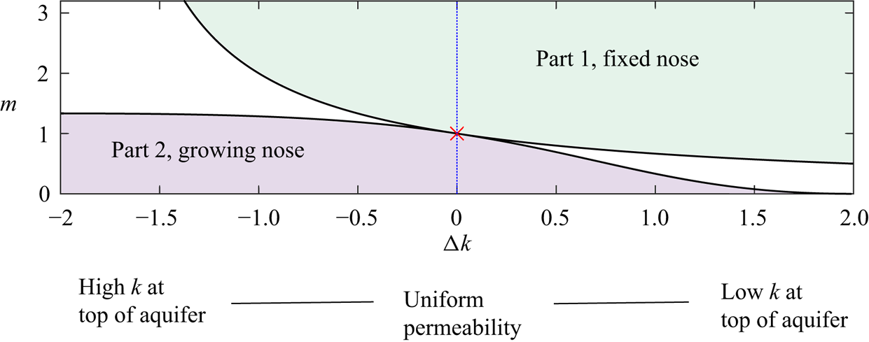
Figure 1. Parameter space from Hinton & Woods (Reference Hinton and Woods2018) for the late-time evolution of the interface between the injected and ambient fluids in the case of linearly varying permeability. The vertical axis corresponds to the viscosity ratio,  $m$, whilst the horizontal axis shows the permeability difference between the top and the bottom of the aquifer ( ${\rm \Delta} k >0$ refers to permeability increasing towards the bottom of the aquifer). In the top right region, corresponding to a high viscosity injectate, the nose has fixed extent and its influence on the migration of tracer is the subject of the present paper. For a low viscosity injectate, the interface grows in proportion to time, $t$. The migration of tracer in that case is studied in Part 2 (Hinton & Woods Reference Hinton and Woods2020). In the intermediate regions (coloured white) the interface has growing regions and fixed regions. For equally viscous fluids in a uniform aquifer, the nose grows in proportion to $t^{1/2}$ (red cross).
Hinton & Woods (Reference Hinton and Woods2019) illustrated that in an aquifer with vertically varying permeability, the shear flow results in the maximum speed of the tracer being faster than the speed of the fixed-extent nose. In the absence of any diffusion, the tracer in the high permeability regions catches and circulates through the flow nose (see figure2). At long times, diffusion becomes important, and leads to cross-layer homogenisation of the tracer. Hinton & Woods (Reference Hinton and Woods2019) studied the purely advective transport, as relevant to relatively thick porous layers for which the cross-layer diffusion time,  $H^{2}/D$, is long compared to the time-scale of the flow, where H is the thickness of the layer (see the region below the dashed line in figure 3). In thinner layers, the cross-flow diffusion may be significant on the time scale of the flow and so the dynamics of the tracer dispersal will be different from the purely advective regime described by Hinton & Woods (Reference Hinton and Woods2019). This forms the subject of the present paper (see figure 3). We combine the physical ingredients of tracer diffusion, an interface zone between the injected and ambient fluid and variation of the rock permeability in the cross-flow direction, which leads to an along-flow shear, which causes some of the tracer to catch up with the nose. The homogenisation owing to cross-flow diffusion occurs before or after tracer reaches the nose leading to different patterns of dispersal. In either case, the tracer eventually becomes vertically homogenised and we investigate the late-time evolution of the tracer distribution and how it is influenced by the interaction with the nose (see figure 3). The different transitions to the late-time vertically well-mixed regimes lead to differences in the ultimate extent of the tracer. Our analysis is developed for any continuously varying permeability structure in the vertical direction but many of our illustrative calculations are carried out using a linear permeability structure.
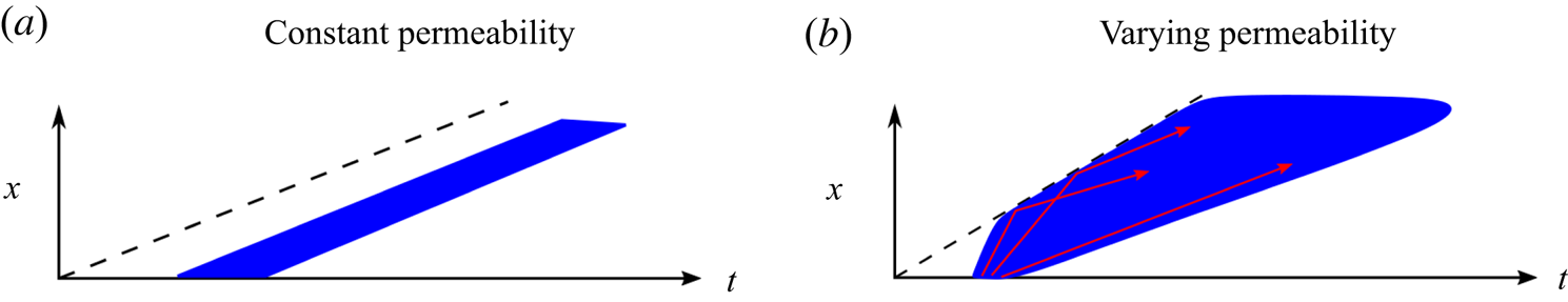
Figure 2. Schematics of the tracer location (blue) relative to the nose (dashed line) in (a) an aquifer with constant permeability and (b) an aquifer with vertically varying permeability. Three tracer paths are shown in (b), illustrating the interaction with the nose.
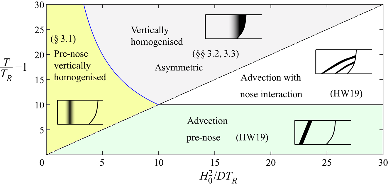
Figure 3. Time regimes for the dispersion of tracer in a intrusion with a fixed shape. The horizontal axis corresponds to the time scale for vertical homogenisation ( $H_0^{2}/D$) relative to the release time of the tracer, $T_R$, whilst the vertical axis is the dimensionless time after release of the tracer. We use illustrative values of the release time and a linear permeability structure with variation relative to the mean permeability of ${\rm \Delta} k=0.1$. The dashed line denotes the time required for vertical homogenisation of the tracer. The pre-homogenised dispersion (below the dashed line) is controlled by the shear flow and interaction with the nose, which was studied by Hinton & Woods (Reference Hinton and Woods2019), denoted as HW19 in the figure. The tracer is sheared prior to interacting with the fixed nose (‘advection, pre-nose’). At a time $L/({\rm \Delta} k V)$ after tracer release, where $L=V T_R$ is the distance of the nose from the initial release, the shearing tracer reaches the nose and is folded (‘advection with nose interaction’). In the next regime, tracer becomes vertically homogenised and spreads from the nose (‘vertically homogenised, asymmetric’). This ordering of regimes occurs in thick aquifers in which $H_0^{2}/D$ is large. In thinner aquifers, vertical homogenisation occurs prior to tracer reaching the nose. Tracer spreads laterally behind the nose in its vertically homogenised regime (‘pre-nose vertically homogenised’). Once homogenised, the rate of dispersion is proportional to $D_{{\textit{eff}}}\sim {\rm \Delta} k^{2} V^{2} H_0^{2}/D$ owing to shear dispersion and the tracer spreads towards the nose, interacting with the nose at a time proportional to $L^{2}/D_{\textit{eff}}$. The curved solid line, corresponding to the interaction between tracer and the nose therefore has shape ${\rm \Delta} k^{-2} (H_0^{2}/DT_R)^{-1}$. The diffusive regimes form the topic of the present paper. The case of pre-nose homogenisation is studied in § 3.1 and the interaction with the nose in §§ 3.2 and 3.3.
The approach in this work is to develop a simplified model for flow through a heterogeneous permeable aquifer so that we can identify the influence of the heterogeneity on the flow, through a single parameter,  ${\rm \Delta} K/\bar {K}$, which is the magnitude of the permeability variation relative to the mean. Although this is idealised, the solutions we derive provide insight into the structure of the flow field, and this is invaluable for interpreting how a pulse of tracer becomes dispersed, but also for interpreting how the injected fluid moves through the permeable layer. In many applications, additives, with time delay, may be used in the flow, in order to change the viscosity or surface tension of the fluids. Understanding the pattern of dispersion is key for successful deployment of such additives, which may ideally be activated when they are at the flow front.
Owing to the many physical processes in the problem we are studying, we begin in § 2 with a brief review of the interface evolution in a confined aquifer with vertically varying permeability (Hinton & Woods Reference Hinton and Woods2018). We introduce a model for the migration of tracer within the injectate. We describe how a finite, vertically uniform pulse of tracer is dispersed within the flow before, during and after its interactions with the nose. We consider linear permeability variations and some example nonlinear permeability variations. We then develop the model in § 5 to account for a non-uniform initial distribution of the tracer owing to the vertical permeability structure. Finally, in § 6, we consider the implications of the combined action of dispersion, shear and the interface zone on inferences made about the rock structure from tracer tests. Our results also have applications beyond tracer tests. The analysis provides detailed understanding of how fluid particles migrate in subsurface displacements where one fluid displaces another. In particular, we show that fluid that is injected later can end up near the front whilst fluid that is injected earlier may fall far behind the front. This knowledge is critical in, for example, informing the addition of viscosifiers to an active injection project.
2. Formulation
If liquid of density  $\rho$ and viscosity $\mu _i$ is injected from a line source at $X=0$ with a flow rate $Q$ into a horizontal, laterally extensive aquifer initially filled with liquid of density $\rho + {\rm \Delta} \rho$ and viscosity $\mu _a$, and the aquifer has depth $H_0$, porosity $\phi$ and permeability $K(Y)$, which varies vertically (figure 4), then the flow is controlled by the combination of the applied pressure associated with the injection and the buoyancy force. We can scale the depth, length and time using the relations
 \begin{equation} h=H/H_0, \quad y=Y/H_0, \quad x = X/H_0, \quad t = QT/(\phi H_0^{2}). \end{equation}
The characteristic buoyancy velocity of the injectate is  $U_B = {\rm \Delta} \rho g \bar {K}/\mu _i$, where $\bar {K}$ is the mean permeability. In this paper, we use capital letters to denote dimensional quantities and lower case for dimensionless quantities, with the exception of the density, the viscosity and gravity, $g$. The dimensionless permeability is
 \begin{equation} k(y) = K(H_0 y)/\bar{K}, \end{equation}
and the viscosity ratio of the two fluids is (see figure 4)
 \begin{equation} m= \mu_i/\mu_a. \end{equation}
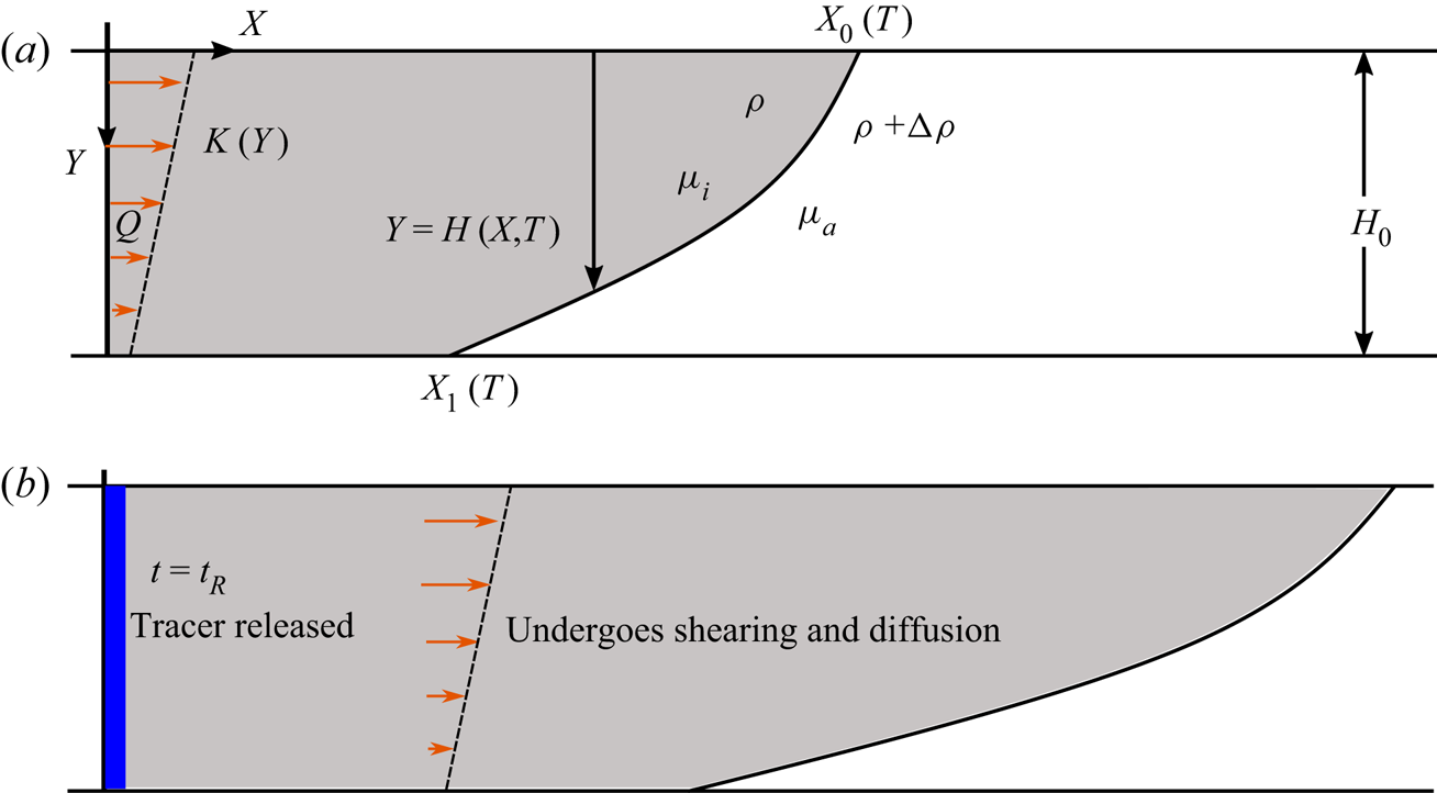
Figure 4. (a) Schematic for the injection of buoyant fluid into a confined aquifer with a vertically varying permeability. (b) A vertically uniform pulse of tracer is released at a time  $t=t_R$ after injection began. The permeability variation creates a shear flow, which leads to shear dispersion.
We assume that the mixing of the two fluids is negligible and that there is a sharp interface between them [see the experimental results of Pegler et al. (Reference Pegler, Huppert and Neufeld2014)]. After an initial transient, the dimensionless Darcy velocity is given by (for details, see Hinton & Woods Reference Hinton and Woods2018)
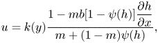 \begin{equation} u = k(y)\frac{1 - mb[1-\psi(h)]\dfrac{\partial h}{\partial x}}{m + (1-m)\psi(h)}, \end{equation}
where
 \begin{equation} \psi(h) = \int_0^{h} k(y)\, \mathrm{d}y, \end{equation}
and  $b=U_B H_0/Q$ is the ratio of the characteristic buoyancy velocity to the injection velocity.
We focus on the evolution of the flow at late times when there is a fully flooded region in which  $h=1$ and a nose region in which $0<h<1$ (see figure 4). Late times correspond to $t \gg b^{-1}$ in dimensionless terms (Zheng et al. Reference Zheng, Guo, Christov, Celia and Stone2015). Hinton & Woods (Reference Hinton and Woods2018) showed that for a sufficiently viscous injectate, the nose advances as a travelling wave with constant shape and velocity (figure 5a). For a linearly varying permeability,
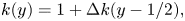 \begin{equation} k(y) = 1 + {\rm \Delta} k (y-1/2), \end{equation}
a fixed nose occurs when (top right region of figure 1)
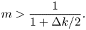 \begin{equation} m > \frac{1}{1+{\rm \Delta} k/2}. \end{equation}
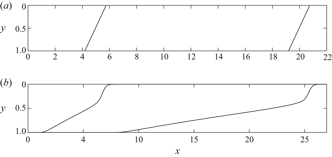
Figure 5. Position of the fluid–fluid interface at  $t=5$ and $t=20$ with $b=1$. (a) For a sufficiently viscous injected fluid relative to the ambient fluid, the nose advances with constant shape and velocity of unity (interface shown is for a constant permeability aquifer, ${\rm \Delta} k=0$, and viscosity ratio, $m=3$). (b) If the viscosity ratio is not so large, the nose can have fixed and growing regions. See also figure 1. We have used $m=0.3$ and ${\rm \Delta} k =1.5$. The interaction between tracer and the ‘mixed’ nose is studied in appendix A.
The lateral extent of the nose is proportional to  $b$. For a less viscous injectate (white regions of figure 1), the nose has a region at the top of the aquifer that travels with constant shape and velocity and a growing region below this (figure 5b). For an even less viscous injectate (bottom left region in figure 1), the entire nose grows in proportion time.
In the present paper, we focus on the migration of tracer in the case that the nose has a fixed shape and extent at late times. The interaction between the tracer and a nose that has a growing region and a fixed region is similar to the case of a fixed nose and the details are given in appendix A. In Part 2 (Hinton & Woods Reference Hinton and Woods2020), we study the migration of tracer in the case that the entire nose grows in time.
2.1. Migration of tracer
We consider the release of a pulse of passive tracer into the input fluid (a continuous release of tracer into the fluid leads to slightly different behaviour, which is described in appendix B). The tracer undergoes diffusion with coefficient  $D$. We assume that the tracer is immiscible in the ambient fluid. The dimensional advection–diffusion equation for the evolution of the concentration of the tracer is
 \begin{equation} \frac{\partial C}{\partial T} + \pmb{U} \boldsymbol{\cdot} \pmb{\nabla} C = D \nabla^{2} C, \end{equation}
where  $\pmb {\nabla \boldsymbol{\cdot} U}=0$ because the injectate is incompressible. In this contribution we focus on the case in which molecular diffusion is the dominant dispersive mechanism, which was found to be accurate for low flow rates by Bear (Reference Bear1961). This simplifies the problem because the diffusion coefficient, $D$, is everywhere a constant.
We make  $C$ dimensionless by scaling it with the initial concentration of released tracer. We scale the diffusion coefficient $D$ with the time scale from (2.1a--d) and the thickness of the aquifer to obtain the dimensionless parameter
 \begin{equation} \mathcal{D} = \frac{\phi D}{Q}. \end{equation}
Note that this is the inverse of the Péclet number,  $\mathcal {D}={{Pe}}^{-1}$.
Behind the nose, the flow velocity (2.4) is  $u=k(y)$ and the vertical velocity is zero by mass continuity. Hinton & Woods (Reference Hinton and Woods2019) showed that, in the absence of diffusion, particles in high permeability regions catch and enter the fixed-extent nose where they migrate into lower permeability regions and fall behind the nose. By considering mass conservation, they showed that particles that enter the nose at $y=y_0$ fall behind and exit the nose at $y=1-y_0$. In the present paper, we assume that if the tracer is well mixed across the vertical extent of the aquifer, then the flux of tracer into the nose at $y_0$ equals the flux out of the nose at $1-y_0$. The time tracer spends in the nose is negligible compared to the time spent behind the nose. Hence, we assume the transition in the nose is instantaneous.
We note that for the lubrication approximation to apply, the cross-aquifer velocity in the nose must be small compared to the along-aquifer velocity, which requires  $b \gg 1$. We also assume that the injection of fluid continues at a constant rate throughout the period in which we study the migration of tracer.
3. Numerical simulations
To simulate the migration of a pulse of tracer numerically, we consider the release of a line of particles from  $x=0$ at $t=t_R$ that then undergo advection and diffusion. We use a particle-tracking numerical method, rather than solving the governing advection–diffusion equation for the concentration, because of the complex geometry of the domain associated with the moving fluid–fluid interface.
The position of a particle satisfies the following dimensionless stochastic differential equation:
 \begin{equation} {\textrm{d}} \boldsymbol{x} = \boldsymbol{u}(\boldsymbol{x},t) \,{\textrm{d}}t + \sqrt{2 \mathcal{D}} \,{\textrm{d}} \boldsymbol{W}(t), \end{equation}
where  $\boldsymbol {u}$ is the flow velocity, $\mathcal {D}$ is the diffusion coefficient and $\boldsymbol {W}$ is a standard two-dimensional Brownian motion. The interface between the injected and ambient fluids, and the aquifer boundaries are treated as no-flux boundaries. We simulate (3.1) numerically using the Euler–Maruyama method (Higham Reference Higham2001). We implement the no-flux condition on the aquifer boundaries, at $y=0$ and $y=1$, by treating it as reflective in the numerical scheme (Erban & Chapman Reference Erban and Chapman2007). The no-flux condition on the moving fluid–fluid interface is implemented as follows. First, the interface position is updated at each time step. Next, the position of the tracer particles are updated. If a tracer particle is outside the injected fluid, then it is reflected in the updated interface. The reflection is via the normal direction to the interface at the point on the interface nearest to the particle. We typically used one million particles to provide a sufficiently accurate distribution and the timestep used was at most $10^{-5}/\mathcal {D}$. The initial release is either vertically uniform (§ 4) or the concentration is proportional to the permeability at each height (§ 5).
4. Release of a uniform pulse
We consider the release of a pulse of tracer into the flow at  $x=0$ at a time, $t=t_R$. The time after release is
 \begin{equation} \tau= t- t_R. \end{equation}
The concentration of tracer within the released pulse is assumed to be uniform across the vertical extent of the aquifer. We study the situation in which the aquifer heterogeneity influences the initial vertical structure of the concentration in § 5.
4.1. Pre-nose migration
We first consider the migration of the tracer at times before the nose has any influence. We study the transition from advection-dominated dispersion at early times to shear dispersion at late times. In this pre-nose regime the flow depth is  $h=1$ and the flow velocities are $u=k(y)$ and $v=0$. At very early times, the tracer spreading is dominated by molecular diffusion. However, this quickly becomes negligible in comparison to the shearing of the tracer pulse owing to the vertical variation of the permeability. We ignore the initial molecular diffusive regime. In the shearing regime, the mean velocity is unity and this motivates transforming the advection–diffusion equation into the travelling frame with $\chi =x-\tau$
 \begin{equation} \frac{\partial c}{\partial t} + \tilde{k}(y) \frac{\partial c}{\partial \chi} = \mathcal{D} \left(\frac{\partial^{2} c}{\partial \chi^{2}} + \frac{\partial^{2} c}{\partial y^{2}} \right), \end{equation}
where  $\tilde {k}(y) = k(y)-1$ is the relative velocity. Note that $\int _0^{1} \tilde {k}(y) {\textrm {d}}y =0$.
At early times, the dispersion of tracer is dominated by the shear flow due to the permeability variation across the aquifer. The lateral extent of the tracer initially grows in proportion to time  $\tau$ and the role of diffusion is negligible (see figure 6a). This advection-dominated dispersion was studied by Hinton & Woods (Reference Hinton and Woods2019). At later times the role of diffusion becomes non-negligible. As the tracer is sheared, large cross-channel concentration gradients develop (see figure 6b). These gradients are smoothed out by diffusion over a time scale of order $1/\mathcal {D}$, which corresponds to the time taken for tracer particles to sample the entire thickness of the aquifer. At times $\tau \gg 1/\mathcal {D}$, the tracer has been sheared and has become ‘well-mixed’ vertically so that the concentration is independent of depth, $y$ (see figure 6d). It has thus spread a much larger lateral distance than it would owing to along-flow diffusion alone, demonstrated by the two columns in figure 6. The combination of the shear flow and cross-channel diffusion enhances the rate of along-flow dispersion. This effect is known as shear dispersion, first explained by Taylor (Reference Taylor1953). To study the distribution of tracer in the along-flow direction, we calculate the moments of the distribution. We follow the method of Aris (Reference Aris1956) and quote the key results below; further details of the full calculations are given in appendix C.
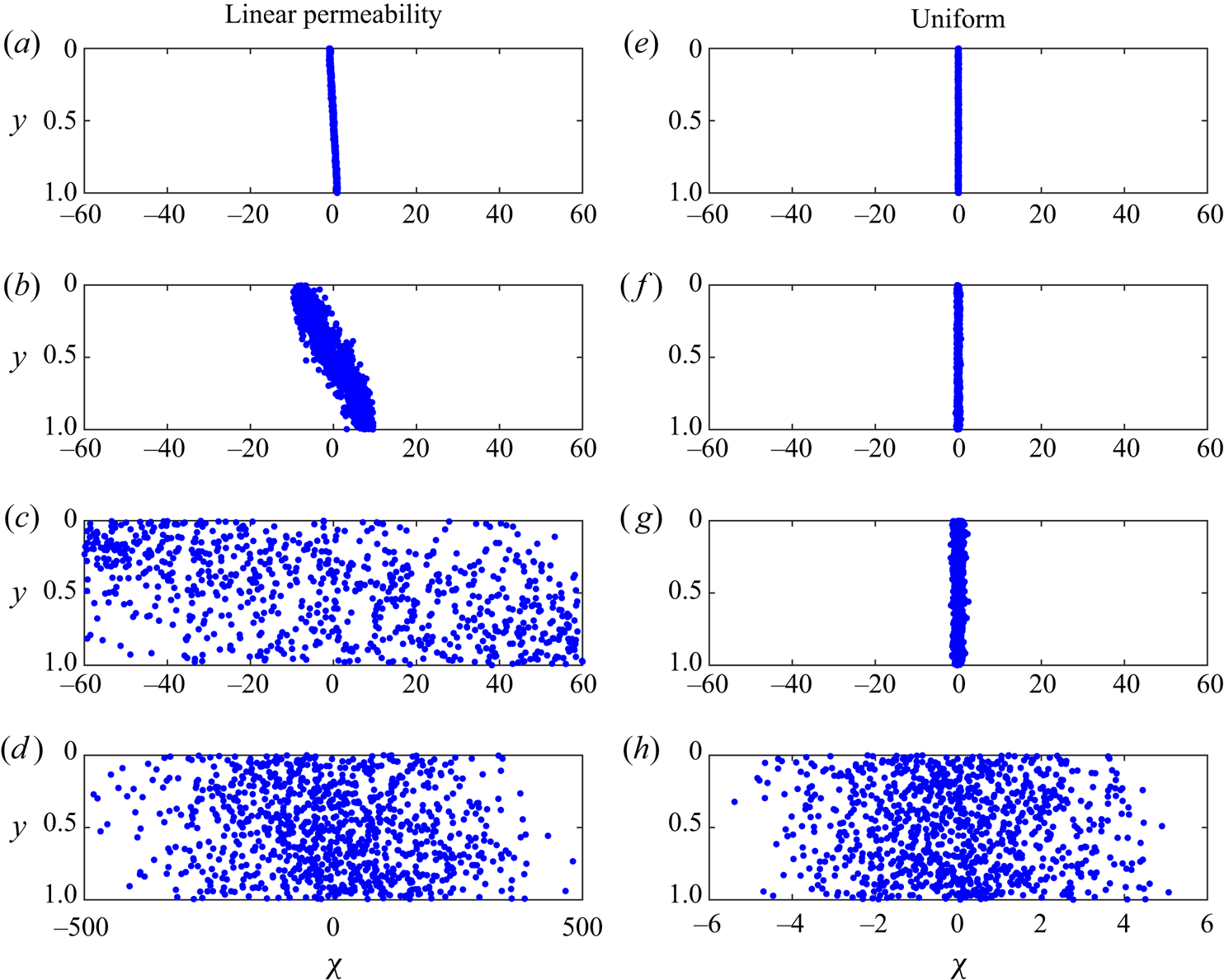
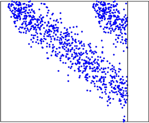
Figure 6. Dispersion of 1000 particles upstream of the nose. (a–d) Dispersion in an aquifer with a vertically linear permeability variation,  ${\rm \Delta} k=1$, and (e–h) in a uniform aquifer. In both cases $\mathcal {D}=0.001$. The rows correspond to four times, in (a, e) $\tau =0.002/\mathcal {D}$, in (b, f) $\tau =0.02/\mathcal {D}$, in (c, g) $\tau =0.2/\mathcal {D}$ and in (d, h) $\tau =2/\mathcal {D}$. In a heterogeneous aquifer, the tracer is sheared by the permeability gradient (see panels (a, b)), which leads to large cross-channel concentration gradients. These are smoothed out by diffusion after times of order $1/\mathcal {D}$ and the tracer distribution becomes independent of cross-channel coordinate. This leads to a much higher dispersion coefficient (see (4.4)) than in a uniform aquifer (note the different axes in (d, h)).
It is straightforward to show that the first moment of the lateral distribution of tracer,  $\chi =m_1(\tau )$, corresponding to the mean position, is fixed in travelling coordinates
 \begin{equation} m_1(\tau) \equiv 0. \end{equation}
At late times,  $\tau \gg 1/\mathcal {D}$, the second moment of the tracer distribution in the lateral direction is given by
 \begin{equation} m_2(\tau) = 2\mathcal{D}_{{\textit{eff}}} \tau - \frac{2\lambda}{\mathcal{D}^{2}}, \end{equation}
where
 \begin{equation} \mathcal{D}_{{\textit{eff}}} = \mathcal{D}+\kappa/\mathcal{D} \end{equation}
is the effective diffusion coefficient, which is an enhanced rate, faster than ordinary molecular diffusion,  $\mathcal {D}$, owing to shear dispersion (compare the two columns in figure6). The constants, $\kappa$ and $\lambda$ depend only on the permeability structure and are given by the following expressions:
 \begin{gather} \kappa = \int_0^{1} \tilde{\psi}(y)^{2} \,\mathrm{d} y, \end{gather}
 \begin{gather} \lambda = \int_0^{1}\tilde{\Psi}(y)^{2} \,\mathrm{d} y, \end{gather}
where
 \begin{equation} \tilde{\psi}(y) =\int_0^{y} \tilde{k}(s) \,\mathrm{d}s, \end{equation}
and  $\tilde {\Psi }(y)$ is the anti-derivative of $\tilde {\psi }(y)$ where the constant of integration is chosen so that $\int _0^{1} \tilde {\Psi }(y)\,\mathrm {d}y=0$.
Since the centre of mass is at  $\chi =0$, (4.4) provides the late-time along-flow variance of the tracer distribution. We plot the predicted variance (4.4) as a red dotted-dashed line in figure 7 for particular parameter values, showing excellent agreement with the numerical results at later times. The dispersion of tracer is symmetric about its centre of mass, provided tracer has not yet dispersed towards the nose. We analyse the interaction between the tracer and the different noses in the next subsections.
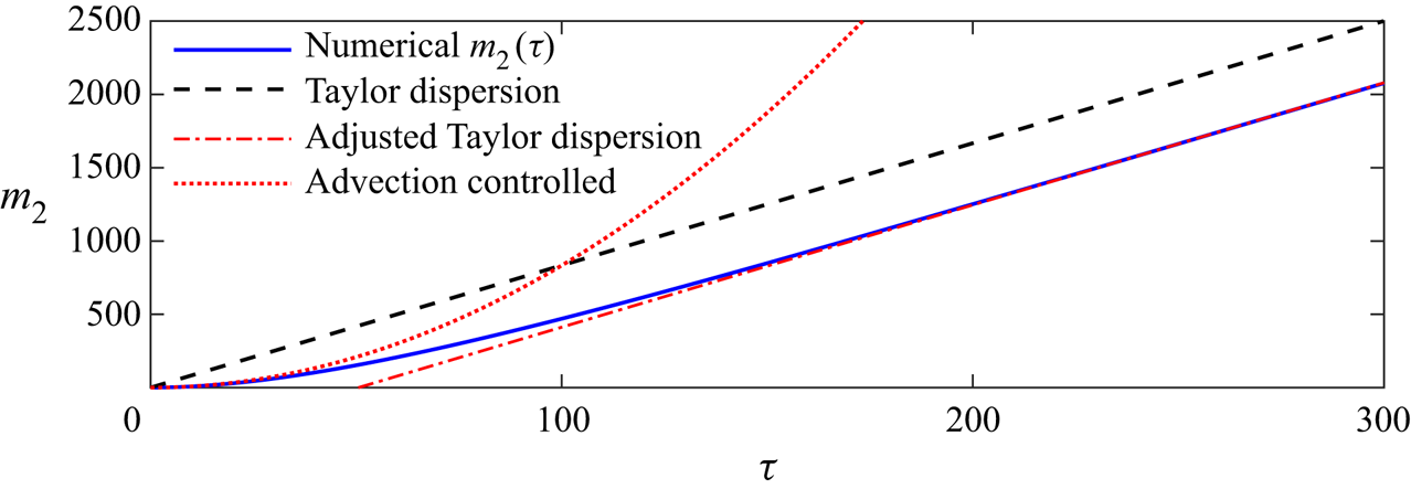
Figure 7. Second moment of the tracer distribution,  $m_2(\tau )$, in the along-channel direction in the case of a linear permeability gradient with ${\rm \Delta} k=1$ and diffusion coefficient, $\mathcal {D}=0.002$. The numerical results are plotted as a solid blue line. The second moment arising from the enhanced Taylor dispersion, $2\mathcal {D}_{\textit{eff}}\tau$, is plotted as a black dashed line. The adjustment owing to the early-time transition to the shear dispersion regime is $-2\lambda /\mathcal {D}^{2}$ (4.4), which is plotted as a red dotted-dashed line showing excellent agreement with the late-time numerical results. The red dotted line represents the early-time dispersion owing to advection in which the second moment of the tracer extent is $({\rm \Delta} k\tau )^{2}/12$.
The analysis of Taylor (Reference Taylor1953) can be used to show that, at late times, the thickness averaged concentration of tracer,  $\bar {c}(\chi ,\tau )$, satisfies the diffusion equation with coefficient $\mathcal {D}_{\textit{eff}}$. At such times, the concentration distribution evolves as a Gaussian with mean $\chi =0$ and variance given by (4.4). The constant term in (4.4) can be interpreted as an adjustment time to the $y$-independent, Gaussian spreading and we write
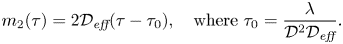 \begin{equation} m_2(\tau) = 2 \mathcal{D}_{{\textit{eff}}} (\tau -\tau_0), \quad \text{where} \ \tau_0 = \frac{\lambda}{\mathcal{D}^{2} \mathcal{D}_{{\textit{eff}}}}. \end{equation}
The constant  $\tau _0$ is a virtual source time for the self-similar Gaussian spreading.
The reduction in the second moment from  $2\mathcal {D}_{\textit{eff}} \tau$ arises because of the early-time behaviour during which the role of diffusion is negligible and the lateral extent of the tracer grows more slowly driven by advection. For example, for a linear permeability gradient,
 \begin{equation} k(y)=1+{\rm \Delta} k (y-1/2), \end{equation}
the second moment evolves according to  $({\rm \Delta} k \tau )^{2} /12$ in the absence of diffusion. This is plotted as a red dotted line in figure 7, and is slower than shear dispersion (dashed black line) at early times.
In order to illustrate the magnitude of shear dispersion in an example heterogeneous layer, consider the permeability profile
 \begin{equation} k(y) = 1 + \frac{{\rm \Delta} k}{2} \left\{ \frac{\tanh[ (x-1/2)/a]}{\tanh[ 1/(2a)]} \right\}, \end{equation}
where  ${\rm \Delta} k$ is the permeability difference between the top and bottom of the aquifer and $a$ is a parameter that quantifies the linearity of the permeability profile (see figure 8a). In the limit $a \to \infty$ the profile (4.11) is linear, given by (4.10), whilst in the limit $a \to 0$ the profile is piecewise constant
 \begin{equation} k(y)= \begin{cases} 1-{\rm \Delta} k/2 & \text{for } y<1/2 \\ 1+{\rm \Delta} k/2 & \text{for } y>1/2 \end{cases}. \end{equation}
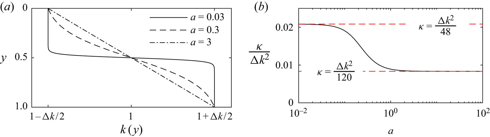
Figure 8. (a) Permeability structure,  $k(y)$, according to (4.11). The profile is linear in the limit $a \to \infty$ and is piecewise constant in the limit $a \to 0$. (b) Shear dispersion coefficient, $\kappa /{\rm \Delta} k^{2}$ as a function of $a$ for the permeability (4.11) (calculated from (4.6)). A linear profile ( $a \to \infty$) has coefficient $1/120$, whilst the piecewise constant profile ( $a \to 0$) has coefficient $1/48$.
In figure 8(b), the contribution,  $\kappa$, to the enhanced diffusion coefficient from the shear is plotted as a function of the parameter $a$ for the permeability profile (4.11). The coefficient $\kappa$ transitions between the two limiting cases of $a\to 0$ and $a \to \infty$. For the piecewise constant profile ( $a \to 0$, (4.12)) we calculate $\kappa ={\rm \Delta} k^{2} /48$ from (4.6). For the linear permeability profile ( $a \to \infty$, (4.10)), $\kappa ={\rm \Delta} k^{2} /120$, which is $2.5$ times smaller than for the profile (4.12).
Note that for a linear profile (4.10),
 \begin{equation} \lambda = \frac{17 {\rm \Delta} k^{2}}{20160}. \end{equation}
4.2. Interaction with the nose post-homogenisation
We consider the interaction of tracer with a fixed nose in the case that the tracer is vertically homogenised before the interaction. We obtain parameter values for which this occurs in § 4.3.
When the tracer is vertically homogenised, its concentration is independent of depth and satisfies the diffusion equation
 \begin{equation} \frac{\partial c}{\partial \tau } = \mathcal{D}_{{\textit{eff}}} \frac{\partial^{2} c}{\partial \chi^{2}}, \end{equation}
where the diffusion coefficient is enhanced owing to shear dispersion ( $\mathcal {D}_{\textit{eff}}>\mathcal {D}$).
The fixed nose spans the thickness of the aquifer and travels at the dimensionless mean flow velocity, which is  $1$. Tracer is released from $x=0$ at $t=t_R$ and the lateral distance between the tracer and the nose is initially $l_R = t_R$. We showed earlier that, for a vertically uniform release of tracer, the centre of mass of tracer travels at the mean flow velocity at times when the nose influence is negligible. Thus, the distance between the nose and the centre of mass remains $l_R$ at these times.
The nose of the current has fixed lateral extent and hence at late times the interface can be approximated as a vertical line, relative to the horizontal length scale of the tracer distribution, which grows in proportion to  $(\mathcal {D}_{\textit{eff}} \tau )^{1/2}$. This assumption is justified further in the application in § 6. Since the tracer is vertically homogenised, the zero-width nose acts as a no-flux boundary to the migration of tracer
 \begin{equation} \left.\frac{\partial c}{\partial \chi} \right\vert_{\chi=l_R} = 0. \end{equation}
Mass conservation of the tracer takes the form
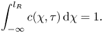 \begin{equation} \int_{-\infty}^{l_R} c(\chi,\tau) \,{\textrm{d}} \chi = 1. \end{equation}
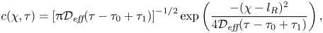
 Equation (4.14) with boundary condition (4.15) and mass conservation (4.16) can be solved following the method of Barenblatt (Reference Barenblatt1996) for heat conduction in a semi-infinite bar. The key idea is that the superposition of the concentration profile of tracer released from  $\chi =0$ and the concentration profile of tracer released from $\chi =2 l_R$ in an infinite domain provides exact solution to the governing diffusion equation with no-flux boundary at $\chi =l_R$ and mass conservation in $\chi < l_R$ at all times after vertical homogenisation. This exact solution is given by the following expression:
 \begin{equation} c = \left[ 4 {\rm \pi}\mathcal{D}_{{\textit{eff}}} (\tau-\tau_0) \right]^{-1/2} \left[ \exp \left( \frac{-\chi^{2}}{4\mathcal{D}_{{\textit{eff}}} (\tau-\tau_0)} \right) + \exp \left( \frac{-(\chi-2l_R)^{2}}{4\mathcal{D}_{{\textit{eff}}} (\tau-\tau_0)} \right) \right], \end{equation}
where the constant  $\tau _0$, given by (4.9), arises from the adjustment to the vertically homogenised regime. This solution is shown at four times as black lines in figure 9(a) and its construction from the superposition of two Gaussians is shown in figure 9(b). At early times of order
 \begin{equation} \tau- \tau_0 \ll \frac{l_R^{2}}{\mathcal{D}_{{\textit{eff}}}}, \end{equation}
the majority of the tracer is far from the nose and the solution (4.17) is well approximated by the following symmetrical Gaussian centred at  $\chi =0$:
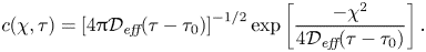 \begin{equation} c(\chi,\tau) = \left[ 4 {\rm \pi}\mathcal{D}_{{\textit{eff}}} (\tau-\tau_0) \right]^{-1/2} \exp \left[ \frac{-\chi^{2}}{4 \mathcal{D}_{{\textit{eff}}} (\tau-\tau_0)} \right]. \end{equation}
This is compared to the exact solution (4.17) at early times in figure 9(a). At later times,  $\tau - \tau _0 \sim l_R^{2}/\mathcal {D}_{\textit{eff}}$, the tracer reaches the nose, and subsequently the distribution changes, owing to the no-flux boundary at this front, assuming the tracer is insoluble in the original fluid in the aquifer. The nose, at $\chi =l_R$, influences the dispersion of the tracer and the concentration distribution becomes asymmetric (see figure 9a). For times much longer than $l_R^{2}/\mathcal {D}_{\textit{eff}}$, the maximum tracer concentration occurs at the nose and the solution (4.17) converges to the half-Gaussian profile
 \begin{equation} c(\chi,\tau) = \left[ {\rm \pi}\mathcal{D}_{{\textit{eff}}} (\tau-\tau_0 + \tau_1) \right]^{-1/2} \exp \left( \frac{-(\chi-l_R)^{2}}{4 \mathcal{D}_{{\textit{eff}}}(\tau - \tau_0+ \tau_1)} \right), \end{equation}
where  $\tau _1$ is a constant associated with the time for a transition to this similarity solution. The half-Gaussian is plotted with red crosses in figure 9(a) and shows good agreement with the solution (4.17) at $\tau -\tau _0=6400$. We determine $\tau _1$ by applying the technique of Barenblatt (Reference Barenblatt1996); the details are given in appendix D, leading to the following result:
 \begin{equation} \tau_1 = \frac{l_R^{2}}{2 \mathcal{D}_{{\textit{eff}}}}. \end{equation}
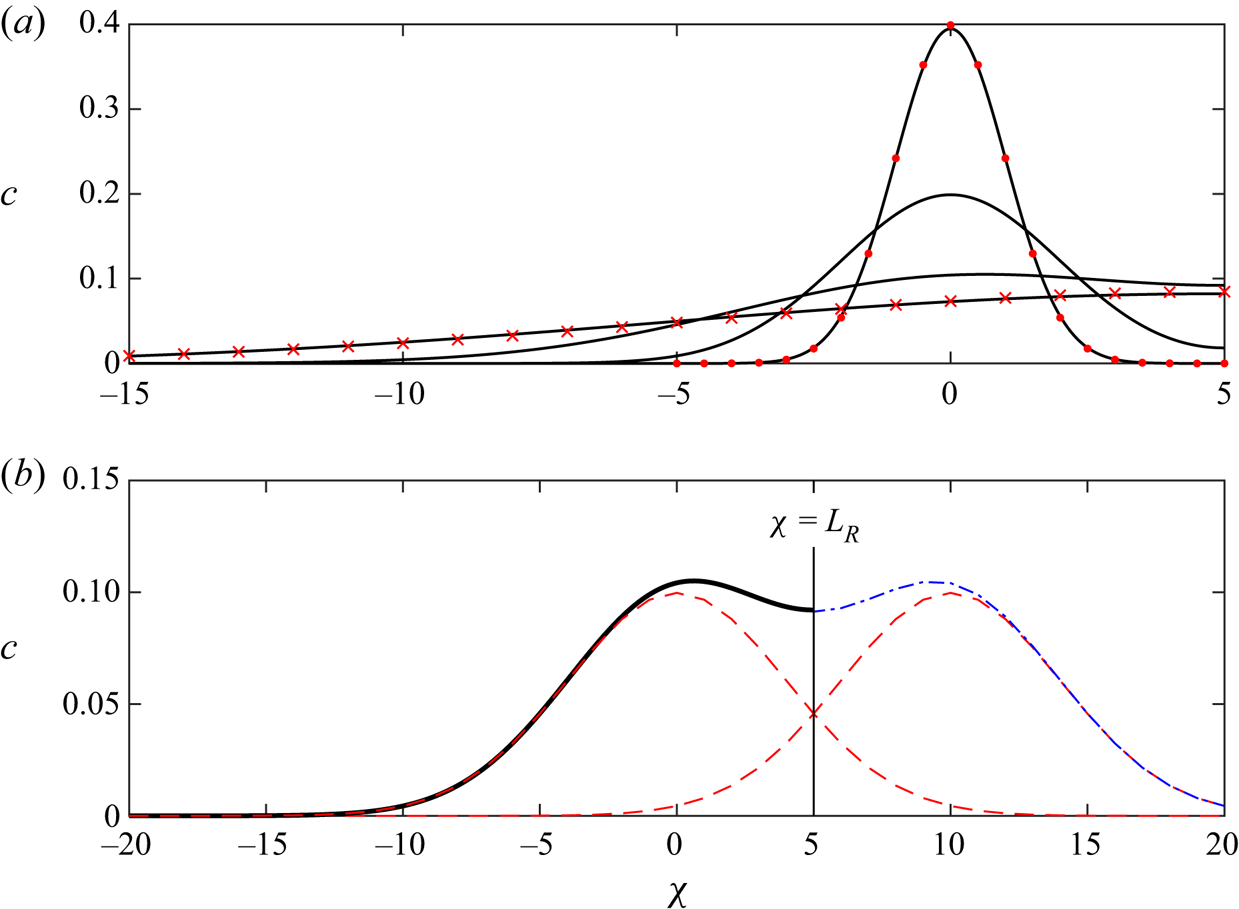
Figure 9. Transition from symmetric dispersion of the vertically homogenised tracer distribution to asymmetric dispersion at late times owing to the interaction with the nose. (a) Transition from Gaussian concentration profile to half-Gaussian with diffusion coefficient  $\mathcal {D}_{\textit{eff}}=0.005$. Black solid lines show the concentration profiles at four times $\tau -\tau _0=100$, $400$, $1600$ and $6400$ obtained from (4.17). We have used $l_R=5$, and hence there is a no-flux boundary at $\chi =5$. The red dots show the Gaussian solution (4.19) and the red crosses show the half-Gaussian solution (4.20). The transition time is $\tau _1=2500$ (see (4.21)). (b) Illustration of Barenblatt's technique for superposing two Gaussian solutions at $\tau -\tau _0=1600$. The red dashed lines show the Gaussian and its reflection in $\chi =5$, the blue dashed line shows the sum of these two Gaussians and the solid black line is the solution in $\chi < l_R$.
The late-time half-Gaussian solution (4.20) is now fully determined, valid for  $\tau -\tau _0 \gg \tau _1$. The time $\tau _1$ is positive because tracer spreads further in the composite solution than it does if tracer were released from the nose at $\chi =l_R$ at time $\tau -\tau _0=0$. During the early symmetric spreading regime, the distance of the centre of mass of tracer behind the interface is a constant, $l_R$. In the half-Gaussian regime, the distance grows in time and is given by
 \begin{equation} \left[4\mathcal{D}_{{\textit{eff}}}(\tau-\tau_0+\tau_1)/{\rm \pi}\right]^{1/2}. \end{equation}
The lateral standard deviation of the tracer concentration transitions from  $(2 \mathcal {D}\tau )^{1/2}$ for symmetric spreading to
 \begin{equation} \left[2(1-2/{\rm \pi}) \mathcal{D}_{{\textit{eff}}}(\tau-\tau_0 + \tau_1)\right]^{1/2} \end{equation}
for the half-Gaussian spreading.
The distance of the centre of mass behind the nose predicted by the composite solution (4.17), which is accurate at all times, is
 \begin{equation} \left[4\mathcal{D}_{{\textit{eff}}}(\tau-\tau_0)/{\rm \pi}\right]^{1/2} \exp[-l_R^{2}/4\mathcal{D}_{{\textit{eff}}}(\tau-\tau_0)] - l_R {{\rm erfc}}[l_R/(4\mathcal{D}_{{\textit{eff}}}(\tau-\tau_0))^{1/2}], \end{equation}
where  ${{\rm erfc}}$ is the complementary error function. This mean is plotted in figure 10(a), for the case $l_R=5$ and $\mathcal {D}_{\textit{eff}}=0.005$, where it is compared to the early-time mean position ( $\chi =0$) and the late-time mean position (4.22). The transition between the time regimes occurs at $\tau -\tau _0 \sim \tau _1$. In figure 10(b), we illustrate how this transition time ( $\tau -\tau _0 \sim \tau _1$) corresponds to tracer reaching the nose by plotting the location of the 90th, 50th and 10th percentiles of the tracer distribution (according to (4.17)) and the location of the nose.
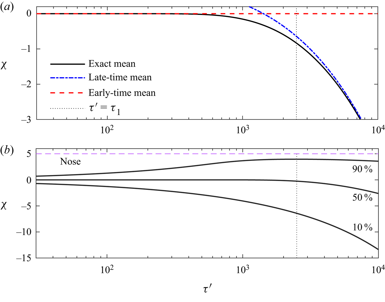
Figure 10. (a) Location of the centre of mass of tracer in travelling coordinates  $\chi =x-\tau$ in the case of a nose of fixed extent initially a distance $l_R=5$ ahead of the tracer. We use diffusion coefficient $\mathcal {D}_{\textit{eff}}=0.005$ and $\tau '=\tau -\tau _0$. The exact position is calculated from the composite solution (4.17), whilst the early- and late-time approximations are calculated from Gaussian spreading (4.19) and half-Gaussian spreading (4.20). (b) Along-channel location of the 90th, 50th and 10th percentiles of the tracer distribution, illustrating how the transition from the early- to late-time regimes occurs (at $\tau ' \sim \tau _1$) when tracer nears the nose.
4.3. Interaction with the nose pre-homogenisation
We have shown how the nose influences the spreading of tracer in the case that tracer is vertically homogenised before reaching the nose. We consider presently the situation in which tracer is not vertically homogenised when it interacts with the nose.
Consider the tanh permeability profile (4.11) with  ${\rm \Delta} k >0$. The permeability is greatest at $y=1$ and the velocity of tracer is $1 + {\rm \Delta} k/2$ there. In the advection-dominated regime ( $\tau \ll 1/\mathcal {D}$), diffusion is negligible and tracer at the bottom of the aquifer ( $y=1$) remains there. In the absence of diffusion, tracer reaches the nose at a time $t=2 l_R/{\rm \Delta} k$ after release.
This time is a good approximation for the arrival of tracer at the nose provided that it is much smaller than the diffusive time scale i.e.  $2 l_R/{\rm \Delta} k \ll \mathcal {D}$. The ratio of these time scales is given by
 \begin{equation} \Gamma = \frac{2 l_R \mathcal{D}}{{\rm \Delta} k} = \frac{2 D T_R}{{\rm \Delta} k H_0^{2}}, \end{equation}
where  $T_R$ is the dimensional release time. The regime $\Gamma \ll 1$ corresponds to advection dominating as tracer in the high permeability region migrates towards the nose. Tracer that enters the nose at a height $y=y_0$ subsequently experiences a non-zero cross-channel velocity. Tracer within the nose migrates across the aquifer into regions of lower permeability where it travels more slowly than the advancing interface. It then lags behind the nose, and in the case of a linear permeability gradient, tracer exits the nose region at a height $1-y_0$ in the absence of diffusion (for details, see Hinton & Woods Reference Hinton and Woods2019). As before, we assume that the transition in the nose happens instantaneously.
The case  $\Gamma \ll 1$ corresponds to a thick layer in which the time for cross-channel diffusion is large. The transition in the nose leads to a reflection of tracer in the centreline and subsequently tracer migrates backwards relative to the nose as illustrated in figures 11(b)–11(d) (corresponding to the white region in figure 3). The extent of the tracer continues to grow in proportion to time, $\tau$, until, at times of order $1/\mathcal {D}$, the tracer becomes vertically well-mixed $c(\chi ,y,\tau ) = \bar {c}(\chi ,\tau )$. Once the tracer concentration is independent of the depth, the nose acts as a no-flux boundary because the flux of tracer in and out the nose balances. The tracer distribution evolves with a half-Gaussian profile, as described earlier (corresponding to the top, grey zone in figure 3). The other case, in which the tracer is vertically homogenised before reaching the nose, corresponding to $\Gamma \gtrsim 1$ (i.e. a thinner aquifer) was discussed in § 4.2 and is illustrated in figures 11(g)–11(j). This regime corresponds to the yellow (leftmost) region in figure 3. Note that the horizontal axis in figure 3 is proportional to $\Gamma ^{-1}$.
Figure 11. Interaction between 1000 tracer particles and a nose of fixed extent at  $\chi =5$. (a) At early times, advection dominates and the tracer undergoes a shear. (b–e) In the case that advection continues to be the dominant dispersion mechanism when tracer nears the nose ( $\Gamma \ll 1$). Tracer is reflected in the centreline by the nose owing to the recirculation in the nose. Subsequently it occupies the low permeability region and migrates backwards relative to the nose. (g–j) If the rate of diffusion is larger then the tracer becomes vertically well mixed before nearing the nose ( $\Gamma \gtrsim 1$). (f, k) For any non-zero value of $\Gamma$, the tracer eventually becomes vertically well mixed. The concentration becomes independent of depth and the nose acts as a no-flux boundary to the depth-integrated concentration, which leads to a half-Gaussian profile for the tracer concentration.
In the case that advection dominates as tracer enters the nose, the tracer in the high permeability half of the aquifer quickly enters the nose (see figure 12). If instead the tracer is vertically homogenised before interacting with the nose then the proportion of particles that have been through the nose evolves more slowly because the concentration near the nose is small and most of the particles are far from the nose (compare figures 12 and 11).
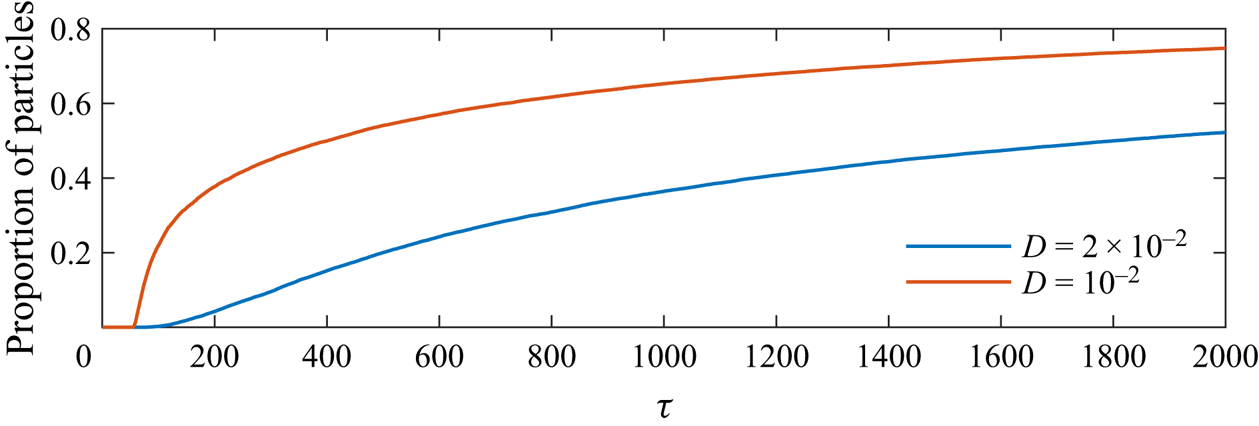
Figure 12. Proportion of tracer particles that have transitioned through the nose at least once. We use a release distance (or time) of  $l_R=25$, a permeability gradient of ${\rm \Delta} k=1$ and two values for the diffusion coefficient $\mathcal {D} = 0.02$ and $\mathcal {D}=0.001$ (corresponding to $\Gamma =1$ and $\Gamma =0.05$, respectively). In the case that $\mathcal {D}=0.001$ (red line), advection dominates and the upper half of the tracer pulse in the high permeability zone quickly enters the nose. For stronger diffusion ( $\mathcal {D} = 0.02$, blue line), the tracer becomes vertically homogenised before reaching the nose and the proportion of particles entering the nose increases much more slowly because only the leading edge of the tracer cloud reaches the nose.
In both regimes ( $\Gamma \ll 1$ and $\Gamma \gtrsim 1$), the ultimate asymptotic behaviour is that the tracer concentration profile becomes depth independent and evolves as a half-Gaussian. The time scale for the extent of the half-Gaussian is
 \begin{equation} \tau + \tau_1 - \tau_0 = \tau + \frac{l_R^{2}}{2\mathcal{D}_{{\textit{eff}}}} - \frac{\lambda}{\mathcal{D}^{2} \mathcal{D}_{{\textit{eff}}}}, \end{equation}
regardless of whether the nose interaction occurs before or after homogenisation. Equation (4.26) can be rewritten in terms of  $\Gamma$; the second and third terms are equal to
 \begin{equation} \tau_1 - \tau_0 = \frac{1}{8 \mathcal{D}_{{\textit{eff}}}} \left( \Gamma^{2} - \Gamma_c^{2} \right), \end{equation}
 where  $\Gamma _c$ is a numerical constant that depends on the permeability structure. For a linear permeability profile, $\Gamma _c = \sqrt {17/2520} = 0.082\ldots$. The time offset for the half-Gaussian, $\tau _1 - \tau _0$ represents the combination of the offset owing to the initial advection-dominated regime ( $\tau _0$) and the offset owing to the interaction with the nose ( $\tau _1$). The former contribution is negative because the advection-driven spreading is slower than the shear dispersion at early times whilst the latter is positive as described above. The offsets balance each other for $\Gamma =\Gamma _c$. Smaller values of $\Gamma$ correspond to advection dominating the dispersion for longer and the late-time extent is reduced. Similarly, for larger values of $\Gamma$, the transition to shear dispersion is much faster and occurs before tracer reaches the nose and the interaction between the shear dispersion and the nose dominates leading to an increased late-time extent.
5. Influence of the permeability variation on the initial release of tracer
In § 4, we assumed that the tracer, released from  $x=0$ at $t=t_R$, was initially uniformly distributed over the thickness of the aquifer. We used this idealised initial condition to simplify the analysis and this enabled us to determine the behaviour of the dominant physical processes in the problem. However, in a heterogeneous aquifer, the initial distribution is unlikely to be uniform; more tracer is released in the higher permeability regions. The flux of tracer released at each height from a vertical line source is proportional to the permeability there. Therefore, the initial concentration of tracer at $x=0$ is $c=k(y)$.
The details of the competition between advection and diffusion described in the previous section is unchanged. However, the mean position of the tracer is altered. When the initial vertical distribution was uniform, the centre of mass of tracer migrated at the mean flow velocity in the advection-dominated early-time regime. In the case that the tracer concentration is initially  $c=k(y)$, the centre of mass of tracer will migrate faster than the mean flow because there is more tracer initially in high permeability regions. For a linear shear (4.10), in the absence of diffusion, the centre of mass is at
 \begin{equation} \int_0^{1} c(t=t_R) u(y) \tau \,{\textrm{d}}y = \tau + \frac{{\rm \Delta} k^{2}}{12} \tau. \end{equation}
 The tracer subsequently becomes vertically well mixed and travels at the mean flow velocity (assuming this occurs before the nose influences the spreading). For the release of a uniform pulse, ignoring the nose influence, the centre of mass of tracer is at  $x=\tau$ during and after the advection-dominated regime. For the heterogeneous pulse, the centre of mass is at $x=\tau + m_1(\tau )$. The correction length, $m_1(\tau )$ arises from the extra velocity above the mean flow during the advection-dominated transition.
To calculate the correction length,  $m_1$, we can again use the method of Aris (Reference Aris1956). The along-aquifer integrated concentration, $c_0(y,\tau )=\int _{-\infty }^{\infty }c \,\mathrm {d}\chi$ satisfies the diffusion equation and has the general solution
 \begin{equation} c_0(y, \tau) = a_0 + \sum_{n=1}^{\infty} a_n \cos( n {\rm \pi}y) \exp \left[-n^{2} {\rm \pi}^{2} \mathcal{D} \tau \right]. \end{equation}
The initial condition,  $c_0(y, 0)=k(y)$ imposes $a_0=1$ and
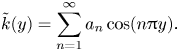 \begin{equation} \tilde{k}(y) = \sum_{n=1}^{\infty} a_n \cos( n {\rm \pi}y). \end{equation}
The equation for the mean position is then given by (cf. (C 4))
 \begin{equation} \frac{\mathrm{d} m_1}{\mathrm{d} \tau} = \sum_{n=1}^{\infty} \int_0^{1} a_n \cos( n {\rm \pi}y) \exp \left[-n^{2} {\rm \pi}^{2} \mathcal{D} \tau \right] \tilde{k}(y)\, \mathrm{d} y. \end{equation}
We integrate with respect to time and apply  $m_1(0)=0$ to obtain
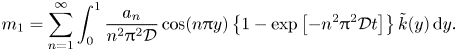 \begin{equation} m_1 = \sum_{n=1}^{\infty} \int_0^{1} \frac{a_n}{n^{2} {\rm \pi}^{2} \mathcal{D}} \cos( n {\rm \pi}y) \left\{1- \exp \left[-n^{2} {\rm \pi}^{2} \mathcal{D} t \right] \right\} \tilde{k}(y) \, \mathrm{d} y. \end{equation}
At times after  $\tau \sim 1/\mathcal {D}$, we neglect the exponential terms. Then integrating by parts twice and substituting (5.3) for the coefficients yields the late-time expression
 \begin{equation} m_1(\tau) = \kappa /\mathcal{D} + \hbox{e.s.t.,} \end{equation}
 where  $\kappa$ is a constant, given by (4.6), and e.s.t. denotes exponentially small terms. This result confirms that the centre of mass of the tracer migrates faster than the mean flow until the tracer has vertically homogenised and this leads to an extra distance of $\kappa /\mathcal {D}$.
We can determine the time dependence of the position of the centre of mass for a linear permeability profile (4.10). We calculate  $a_{2m+1} = -4{\rm \Delta} k/[(2m+1)^{2} {\rm \pi}^{2}]$ and $a_{2m}=0$ from (5.3). The distance that the centre of mass is ahead of the mean flow is
 \begin{equation} m_1(\tau) = \frac{1}{\mathcal{D}} \sum_{n=1}^{\infty} \frac{8 {\rm \Delta} k^{2}}{(2m+1)^{6} {\rm \pi}^{6}} \left\{ 1- \exp[-(2m+1)^{2} {\rm \pi}^{2} \mathcal{D} \tau] \right\}, \end{equation}
which converges to  $\kappa /\mathcal {D}={\rm \Delta} k^{2}/(120\mathcal {D})$ as expected. The adjustment $m_1(\tau )$ is plotted in figure 13 for the case of a linear permeability profile with ${\rm \Delta} k=1$ and $\mathcal {D}=0.002$. The mean from the numerical results, with two million particles, is plotted as a solid blue line and the first hundred terms of (5.7) are plotted with red dots showing excellent agreement (for details of the numerical approach, see § 3).
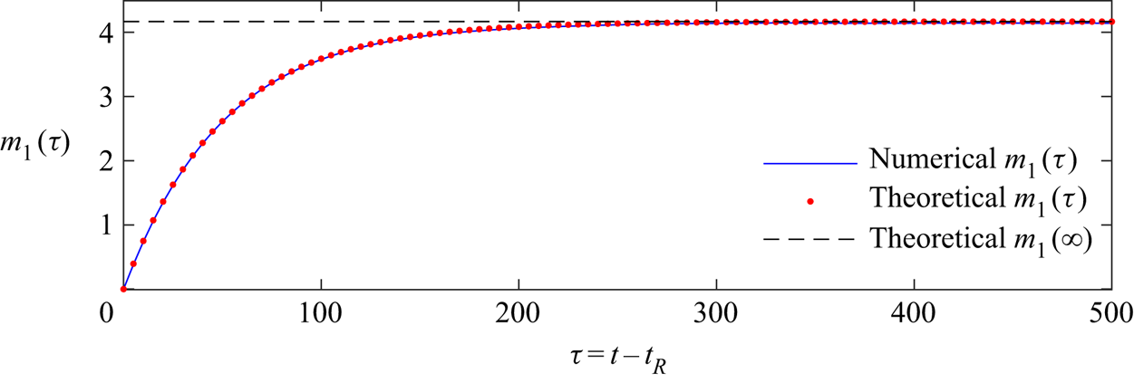
Figure 13. Distance of the centre of mass ahead of the mean flow,  $m_1(\tau )$ owing to the initial non-uniform concentration profile, $c_0(y,0)=k(y)$ in the case of a linear permeability profile with ${\rm \Delta} k=1$ and diffusion coefficient $\mathcal {D}=0.002$. The mean position calculated from our numerical simulations (see § 3) with two million particles is plotted as a blue line whilst the theoretical prediction from the first hundred terms of (5.7) is plotted as red dots. The black dashed line is the late-time limit $m_1 = \kappa /\mathcal {D}$.
We have found how the position of the centre of mass is advanced owing to the higher proportion of tracer in the high permeability region during the early-time transient in the case that the nose does not influence the migration during this period.
6. Applications
We consider the release of tracer in two example aquifers of differing thickness and illustrate how this changes the processes that dominate the dispersion of tracer. In both cases we assume that the input fluid is sufficiently viscous that the interface advances with fixed shape. This may be the case in contexts such as enhanced oil recovery or geothermal power extraction in superheated reservoirs, although any phase change will further complicate the results (cf. Woods Reference Woods1999).
We take the coefficient of molecular diffusion in a porous medium to be  $D = 5 \times 10^{-9}\ \textrm {m}\ \textrm {s}^{-2}$ (Woods Reference Woods2015). We use a typical value for the injection velocity within the layer of $V_i=Q/ (\phi H_0) = 2 \times 10^{-5}\ \textrm {m}\ \textrm {s}^{-1}$. Shear dispersion becomes important at times when tracer is vertically homogenised, which corresponds to $T \sim H_0^{2} /D$.
First, we consider a layer with thickness of  $10\ \textrm {m}$. The time scale for vertical homogenisation is centuries. The advection owing to the shear flow associated with any permeability variation will dominate the dispersion of tracer in the months and years after its release. In figure 14(a), the lateral standard deviation is plotted against time. In the two cases plotted, tracer is released one week and five weeks after the start of injection and we assume the layer has a linear permeability profile with ${\rm \Delta} k=1$. At early times after release, the extent of tracer grows linearly in time owing to the shear flow. At later times, the tracer in high permeability regions enters the nose and the tracer is reflected in the centreline ( $y=1/2$) as it interacts with the nose. This still leads to linear growth of the extent but the constant is altered. For a larger release time, the tracer is initially further behind the nose and the nose interaction occurs at a later time. The role of diffusion is negligible in the case of a fixed nose in a $10\ \textrm {m}$ layer over the typical time scales of a project.
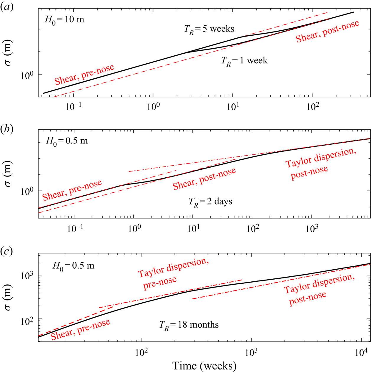
Figure 14. Evolution of the lateral standard deviation of tracer ( $\sigma$) as a function of time (solid black lines). (a) A $10\ \textrm {m}$ layer, (b, c) a $0.5\ \textrm {m}$ layer. Parameter values are given in the text and in both cases the injection velocity is $2 \times 10^{-5}\ \textrm {m}\ \textrm {s}^{-1}$. In (a), the spreading is dominated by advection associated with the shear flow with $\sigma \sim T$. The coefficient changes as tracer interacts with the nose and is transported into lower permeability regions (indicated by the dashed red lines). Two release times are shown. Vertical homogenisation (and hence shear dispersion) does not occur until centuries have passed. (b) In a thinner layer, the early spreading is similar to the thicker layer and tracer reaches the nose. However, at later times ( $H_0^{2}/D$), Taylor dispersion dominates and $\sigma \sim T^{1/2}$ (red dot-dashed line). The coefficient for the rate of this post-nose Taylor dispersion is given by (4.23). (c) For a much later release time in the thin layer, Taylor dispersion dominates before the interaction with the nose.
The permeable layer could have thickness as low as a few centimetres. If we consider a layer of thickness  $0.5\ \textrm {m}$ then the time scale for vertical homogenisation of the tracer is of order
 \begin{equation} H_0^{2} /D = 5 \times 10^{7}\ \textrm{s} = 19\ \text{months}. \end{equation}
If the  $0.5\ \textrm {m}$ layer has a linear permeability structure with ${\rm \Delta} k=1$, then the dimensional shear dispersion coefficient is
 \begin{equation} D_{{\textit{eff}}} = D + \frac{\kappa H_0^{2} V_i^{2} {\rm \Delta} k^{2}}{D} = 1.7 \times 10^{-4} \ \textrm{m}\ \textrm{s}^{-2}. \end{equation}
This is almost five orders of magnitude larger than the molecular diffusion coefficient.
We consider tracer released into this layer two days after the injection began. We suppose that the injection velocity in the thinner layer remains,  $V_i=Q/ (\phi H_0) = 2 \times 10^{-5}\ \textrm {m}\ \textrm {s}^{-1}$. In figure 14(b), we plot the standard deviation against time. At very early times, advection dominates and the extent grows in proportion to time as in the $10\ \textrm {m}$ layer. Tracer is then transported into lower permeability regions by the nose and there is slower linear growth. Subsequently, tracer becomes vertically homogenised and shear dispersion dominates the spreading. In this regime, the extent grows in proportion to $T^{1/2}$. The behaviour of the dispersion of tracer is substantially changed in layers of different thicknesses. In both examples, we assumed that the tracer release was vertically uniform. A vertical variation in the initial concentration alters the mean position by approximately 10 m. We note that in the case of a very late release time, the tracer becomes vertically homogenised before the interaction with the nose (figure 14c).
In figure 15, the concentration profiles that would be observed at a well a distance  $100$ m downstream from the injection well are shown for the cases discussed above. The transition from the shearing pre-nose regime to the shearing post-nose regime can be observed by comparing figures 15(a) and 15(b). In this $10$ m thick layer, diffusion is unimportant. In the case that tracer is released a week after $\textrm {CO}_{2}$ injection begins (figure 15a), tracer in the high permeability regions reaches the nose and is transported into the low permeability regions. There is then a region near the nose in which the tracer concentration is doubled (cf. figure 11c). This region ends abruptly after about 12 weeks as can be observed. For a later release, there is no interaction with the nose and the concentration reduces in time as the tracer in low permeability regions slowly reaches the observation well.

Figure 15. Arrival times of tracer at an observation well that is  $100$ m downstream for the cases considered in figure 14. The parameter values are given in the text. The arrival time is measured from the time at which tracer is released. (a, b) In the thick layer ( $H_0=10$ m) the role of diffusion is negligible and the tracer undergoes a shear. For an earlier release time, the tracer reaches the nose and is ‘folded’, which leads to a region in which the concentration is double the upstream concentration (cf. figure 11c) as seen in panel (a). With a later release time, the tracer has not interacted with the nose when it reaches the observation well. (c, d) In a thinner layer, cross-flow diffusion vertically homogenises the tracer. For an earlier release time, tracer interacts with the nose developing a half-Gaussian profile. The greatest concentration is at the front of the cloud of tracer, which coincides with the nose. For a later release time, the tracer has not interacted with the nose and the maximum concentration is not at the front of the tracer cloud.
The transition from the Taylor-dispersion pre-nose regime to the Taylor-dispersion post-nose regime can be observed by comparing figures 15(c) and 15(d). In this  $0.5$ m layer, cross-flow diffusion is important. For an early release, the half-Gaussian regime develops as tracer interacts with the nose and the highest concentration is at the front (figure 15c). For a much later release of tracer, the nose does not affect the dispersion and the maximum concentration is not at the front. Also, the arrival time (measured from the tracer release time) is much longer for earlier releases because the nose acts as a no-flux boundary slowing the dispersal of tracer towards the observation well (compare the axes in the two columns in figure 15). We have demonstrated that the different regimes analysed in this paper can lead to substantially different observed concentration profiles and hence understanding the dispersal mechanisms is key to correctly interpreting the results of tracer tests.
Finally, we justify our assumption that the extent of the fixed nose is negligible in comparison to the lateral extent of the tracer and hence the nose can be modelled as a vertical line of zero width. The length scale that tracer disperses in the shear dispersion regime over a year is  $(2 D_{\textit{eff}} T)^{1/2} \sim 100\ \textrm {m}$. In the purely advective regime in an aquifer with vertically varying permeability, the length scale after a year is ${\rm \Delta} k V_i T/\sqrt {12}=180\ \textrm {m}$ in the case that ${\rm \Delta} k =1$. The fixed nose has extent proportional to $b H_0$, where $b=U_B H_0/Q$ is the ratio of the buoyancy velocity to the injection velocity. Consider an aquifer with mean permeability $4 \times 10^{-13}\ \textrm {m}^{2}$, porosity $\phi =0.2$, input fluid viscosity of $6 \times 10^{-5}\ \textrm {Pa}\ \textrm {s}$ and density difference between the fluids of $300\ \textrm {kg}\ \textrm {m}^{-3}$. Then the buoyancy velocity is $U=2\times 10^{-5}\ \textrm {m}\ \textrm {s}^{-1}$ and $b=5$ so that the nose extent is of order metres compared to the dispersive length scale over a year, which is hundreds of metres in the advection-dominated or shear dispersion regimes.
In this section, we have assumed that the permeability in the aquifer varies linearly with depth. This is a good first approximation for many real aquifers and both the qualitative and quantitative results we have obtained regarding the role of advection, diffusion, shear dispersion and the nose region apply generally to any permeability variation (see for example figure 8).
6.1. Application to chemical additives
There are several applications in which chemical additives are included in the injection fluid in order to change the properties of the flow within a reservoir. For example, in enhanced oil recovery, the objective is to displace more of the oil in place in the reservoir so that the overall efficiency of the recovery system is increased. If the region near the injection well has already been swept, then ideally chemicals which are added to the system to alter the behaviour of the injected fluid would be activated near the leading front of the injected fluid, so that they have the maximum impact, rather than simply injecting a more viscous fluid since this will first displace the region near the injection well, which has already been swept; there is also the danger of degrading the permeability near the injection well if active chemicals are injected directly into the reservoir, whereas delayed action of these chemicals deeper in the reservoir can help to mitigate this risk. It is possible to use a delayed trigger to activate the additives in the injected fluid, for example using an encapsulation system (Yow & Routh Reference Yow and Routh2009) but how one can place the additive near the flow front in the event that it is injected some time after the start of the injection process is less clear. The present analysis identifies that the heterogeneities of the system may naturally lead to a shear and hence enable some of the newly injected fluid to reach the flow front, where the chemical additive can be activated. By using a tracer with an observation well, testing could be carried out to constrain the magnitude of the shear associated with the fluctuations in the permeability, and thereby help to inform the design of such an enhanced treatment process.
7. Conclusion
In this contribution, we have analysed the migration of tracer within a fluid injected into a confined aquifer initially saturated with a second fluid of different viscosity. The analysis focuses on the dispersion of tracer driven by the combination of a shear flow, which arises from permeability variations, molecular diffusion and interaction with the fixed-extent interface region. The evolution of the tracer distribution is initially advection controlled and the extent grows in proportion to  ${\rm \Delta} k V T$ owing to the shear, which has magnitude ${\rm \Delta} k$ ( $V$ is the injection velocity). At later times, of order $H_0^{2}/D$, cross-channel diffusion has vertically homogenised the tracer distribution leading to an enhanced dispersion coefficient with the lateral extent of tracer growing in proportion to $[2(D+\kappa V^{2} H_0^{2}/D) T ]^{1/2}$, where $\kappa$ is a dimensionless constant, which is a function of the permeability structure.
We have shown how tracer interacts with the nose region of the flow in the case that it has fixed extent and travels at the mean injection velocity, which occurs provided the input fluid is sufficiently viscous relative to the ambient. Tracer may reach the nose during the advection-dominated regime or during the vertically homogenised regime. We have shown that in both cases the tracer distribution transitions from symmetric to asymmetric. The concentration distribution tends to a half-Gaussian, with the maximum concentration at the nose.
The initial release of tracer may not be vertically uniform but instead the concentration released at each height may be proportional to the permeability there. This alters the results because there is a transition in which the tracer migrates ahead of the mean flow since more tracer is released in higher permeability regions. We have quantified the extent of the distance advanced ahead of the mean flow.
We have applied our results in the context of subsurface flows, demonstrating that, depending primarily on the thickness of the aquifer, the migration of tracer is controlled by advection in thicker layers whilst shear dispersion is the dominant mechanism in thinner layers. The difference is important for accurately interpreting the results of tracer tests. In the case that advection dominates, the concentration observed at a production has a significant discontinuity if the tracer has interacted with the nose owing to the ‘folding’ associated with the nose. In a thinner aquifer, the concentration observed will increase and then decrease if the tracer has not yet interacted with the nose or will slowly decrease in time if the half-Gaussian regime has developed following interaction with the nose. Our results also suggest that encapsulated chemical agents could be added to the injected fluid at later times but still reach the front of the displacement, where they may be activated to, for example, alter the viscosity or surface tension.
In Part 2, we consider the case of a growing nose when the injected fluid is of relatively low viscosity (Hinton & Woods Reference Hinton and Woods2020).
Acknowledgments
The authors wish to thank T. Espie for his support of this work, and BP and EPSRC for the award of a CASE studentship funding the research.
Declaration of interests
The authors report no conflict of interest.
Appendix A. Mixed nose
We consider here the migration of tracer in the case that the interface consists of a growing region and a region of fixed extent (see figure 5b). This situation does not occur in a uniform aquifer. The results are different to those in a full growing nose because the thickness of the current does not tend to zero; shear dispersion remains important. The fixed region provides a boundary to the migration of tracer, similar to the full fixed interface.
The fixed region is downstream of the growing region and advances with constant velocity  $v_s>1$ and height $h_s < 1$ (see figure 16). The growing region is supplied by fluid from upstream. Tracer enters the growing region where it has horizontal velocity (2.4)
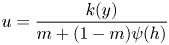 \begin{equation} u = \frac{k(y)}{m + (1-m)\psi(h)} \end{equation}
because the influence of buoyancy is neglected. The tracer becomes vertically homogenised owing to the cross-channel diffusion and reaches the nose (see figure 16). The extent of tracer grows in proportion to  $t^{1/2}$ whilst the nose grows in proportion to $t$. Therefore, in the region occupied by the tracer, the thickness of the flow is approximately a constant, equal to the thickness of the fixed region, $h_s$.
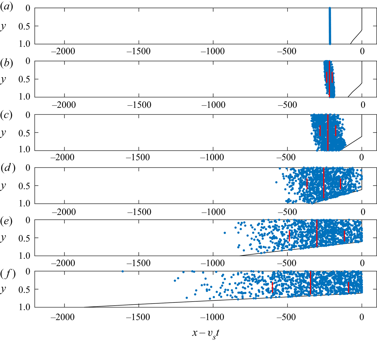
Figure 16. The positions of 1000 particles relative to the mixed interface at six times. (a) Particles at release. (b) Dispersion dominated by advection owing to the shear. (c) Shear dispersion becomes important. (d) Particles become vertically well mixed; the direction of the shear can no longer be seen. Particles begin to spread to the interface. (e, f) The interface provides a no-flux boundary and the distribution becomes asymmetric. The mean distance of tracer behind the fixed nose region is a constant until tracer spreads to the interface.
We expect shear dispersion, driven by the cross-channel linear variation in velocity, to play an important role in the along-channel dispersion of tracer. Near the fixed region, the velocity difference across the tracer distribution is
 \begin{equation} {\rm \Delta} u = \frac{{\rm \Delta} k h_s}{\psi(h_s) + m(1-\psi(h_s))}. \end{equation}
The contribution to longitudinal dispersion from the linear shear is
 \begin{equation} \frac{{\rm \Delta} u^{2} h_s ^{2}}{120 \mathcal{D}} = \frac{{\rm \Delta} k^{2} h_s^{4}}{120 [\psi(h_s) + m(1-\psi(h_s))]^{2} \mathcal{D}} = \frac{v_s ^{2} {\rm \Delta} k^{2} h_s^{4}}{120 [1+{\rm \Delta} k(h_s -1) ]^{2} \mathcal{D}}. \end{equation}
Note that the depth,  $h_s$, and the position of the leading contact point, $v_s t$, depend on ${\rm \Delta} k$ and $m$ (see Hinton & Woods Reference Hinton and Woods2018). In the limit that the mixed nose becomes a full fixed nose, where the fixed region deepens to occupy the entire aquifer, $h_s \to 1$ and $v_s \to 1$, we recover the coefficient for the full fixed region
 \begin{equation} \frac{{\rm \Delta} k^{2}}{120 \mathcal{D}}. \end{equation}
The effective dispersion coefficient in the mixed nose is
 \begin{equation} \mathcal{D} + \frac{v_s ^{2} {\rm \Delta} k^{2} h_s^{4}}{120 [1+{\rm \Delta} k(h_s -1) ]^{2} \mathcal{D}}. \end{equation}
Appendix B. Continuous release of tracer in the case of a fixed nose
In some applications, tracer may be continuously added to the injectate from a time  $t=t_R$ onwards, rather than instantaneously releasing a pulse of tracer. For example, in enhanced oil recovery it may be the case that the source of injected water is changed and the new water contains a solute or a different polymer is added to the water sometime after injection begins. To understand the migration of tracer in this case we can use the model from § 2; we use the concentration of tracer in the input fluid as the scale for $C$ so that in dimensionless terms $c=1$ at release.
We consider the migration of tracer post-homogenisation and neglect the adjustment time to this regime. The evolution of the tracer concentration evolves according to the diffusion equation with coefficient  $\mathcal {D}_{\textit{eff}}$ and boundary condition $c \to 1$ as $\chi \to -\infty$ and initial condition $c=0$ for $\chi >0$. At times when the influence of the nose on the tracer migration is negligible, the system has a similarity solution with
 \begin{equation} c = f(\eta), \quad \eta = \chi / (\mathcal{D}_{{\textit{eff}}} \tau)^{1/2}. \end{equation}
This can be recast as
 \begin{equation} c(\chi, \tau ) = \frac{1}{2} {erfc} \left[\chi/(4\mathcal{D}_{{\textit{eff}}}\tau)^{1/2} \right]. \end{equation}
The tracer diffuses towards the fixed nose and, as discussed in the main text, at later times the nose acts as a no-flux boundary
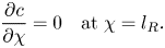 \begin{equation} \frac{\partial c}{\partial \chi}=0 \quad \text{at} \ \chi = l_R. \end{equation}
By considering the fluid injected before the release of tracer, we can obtain the conservation of mass condition
 \begin{equation} \int_{-\infty}^{l_R} (1- c) \,{\textrm{d}} \chi = l_R. \end{equation}
At times long after tracer has reached the nose, the dispersion of tracer becomes independent of the initial distance between the tracer and the nose,  $l_R$. The tracer subsequently spreads in a self-similar fashion with the length scale from the nose growing in proportion to $(\mathcal {D}_{\textit{eff}} \tau )^{1/2}$. Combining this with the boundary conditions, (B 3) and $c \to 1$ as $\chi \to -\infty$ and mass conservation (B 4) motivates the similarity variables
 \begin{equation} c= 1 - \left[\mathcal{D}_{{\textit{eff}}} (\tau+\tau_1) \right]^{-1/2} g (\xi) {,}\quad \xi = (\chi -l_R)/\left[\mathcal{D}_{{\textit{eff}}} (\tau+\tau_1) \right]^{1/2}, \end{equation}
where, analogous to the finite release,  $\tau _1$ is a constant associated with the time for a transition to this similarity solution. The shape function $g(\xi )$ has boundary conditions $g\to 0$ as $\xi \to -\infty$ and $g'(0)=0$, with mass conservation
 \begin{equation} \int_{-\infty}^{0} g \,{\textrm{d}} \xi = l_R. \end{equation}
The late-time solution for the concentration is
 \begin{equation} c = 1 - \frac{l_R}{\sqrt{{\rm \pi} \mathcal{D}_{{\textit{eff}}} (\tau + \tau_1) }} \exp \left[ \frac{(\chi-l_R)^{2}}{4\mathcal{D}_{{\textit{eff}}}(\tau+\tau_1)} \right]. \end{equation}
 We observe that Barenblatt's technique of superposing two early-time solutions can be utilised again. Consider the release of tracer in  $\chi <0$ and $\chi > 2 l_R$, then the concentration is (see (B 2))
 \begin{equation} c = \frac{1}{2} {{\rm erfc}} \left[\chi/(4\mathcal{D}_{{\textit{eff}}}\tau)^{1/2} \right] + \frac{1}{2} {{\rm erfc}} \left[(2l_R-\chi)/(4\mathcal{D}_{{\textit{eff}}}\tau)^{1/2} \right], \end{equation}
which satisfies the initial conditions, mass conservation and the boundary conditions;  $c \to 1$ as $\chi \to -\infty$ and $\partial c/\partial \chi =0$ at $\chi =l_R$. In fact, (B 8) provides an exact solution for the tracer concentration at all times. We plot the concentration at four times in figure17, using (B 8).
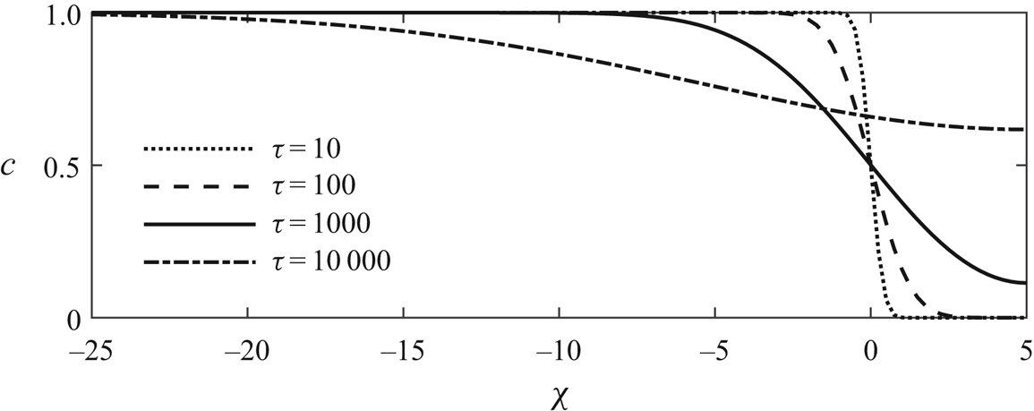
Figure 17. Concentration of tracer in travelling coordinates,  $\chi = x- \tau$, for the continuous release of tracer in $t\ge t_R$. The fixed travelling interface between the two fluids is at $\chi =l_R=5$ and $\mathcal {D}_{\textit{eff}}=0.005$. The concentration is calculated using the superposition technique (B 8) and plotted at four times.
To determine the constant,  $\tau _1$, we compare the superposed solution (B 8) with the late-time solution (B 7) in the same limits as in § 4. We expand (B 7) as a series in $\tau _1/\tau \ll 1$ and (B 8) as a series in $l_R/(\chi -l_R) \ll 1$ in order to obtain
 \begin{equation} \tau_1 = l_R^{2} /6\mathcal{D}. \end{equation}
Appendix C. Calculation of the moments of the tracer concentration distribution prior to the interaction with the nose
To study the distribution of tracer in the along-flow direction, we calculate the moments of the distribution. We follow the method of Aris (Reference Aris1956) and define
 \begin{gather} c_p(y,\tau) = \int_{-\infty}^{\infty} \chi^{p} c(\chi, y, \tau) \,\mathrm{d} \chi, \end{gather}
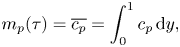 \begin{gather}m_p(\tau) = \overline{c_p} = \int_0^{1} c_p \,\mathrm{d} y, \end{gather}
for any integer  $p$. We can obtain an equation for $c_p$ by multiplying (4.2) by $\chi ^{p}$ and integrating over the entire extent of the aquifer (assuming the nose is far from the zone occupied by the tracer)
 \begin{equation} \frac{\partial c_p}{\partial \tau} = \mathcal{D} \frac{\partial^{2} c_p}{\partial y^{2}} + \mathcal{D} p(p-1) c_{p-2} +p \tilde{k}(y) c_{p-1}. \end{equation}
Then, integrating over the thickness of the aquifer yields
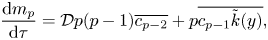 \begin{equation} \frac{\mathrm{d} m_p}{\mathrm{d} \tau} = \mathcal{D} p(p-1) \overline{c_{p-2}} + p \overline{ c_{p-1} \tilde{k}(y) }, \end{equation}
where an overline represents the integral:
 \begin{equation} \overline{\phi}(\chi, \tau)=\int_0^{1} \phi(\chi, y, \tau)\, {\textrm{d}}y. \end{equation}
Since a vertically uniform pulse of tracer is released from  $\chi =0$ at $\tau =0$ we obtain the following initial conditions:
 \begin{gather} c_0(y,0) = 1, \quad c_p(y,0) =0 \quad \text{for}\ p \ge 1, \end{gather}
 \begin{gather}m_0(0) = 1, \quad m_p(y,0) =0\quad \text{for}\ p \ge 1. \end{gather}
Note that  $m_0(\tau ) \equiv 1$ owing to conservation of tracer. We also have the boundary conditions $\partial c_p/ \partial y =0$ at $y=0$ and $y=1$ as there is no flux into the boundary.
The equation for  $c_0$ is (see (C 3))
 \begin{equation} \frac{\partial c_0}{\partial \tau} = \mathcal{D} \frac{\partial^{2} c_0}{\partial y^{2}}. \end{equation}
Combining (C 8) with the initial condition (C 6), we obtain  $c_0(y,\tau ) \equiv 1$. Substituting this into the equation for the first moment (C 4) yields $m_1(\tau ) \equiv 0$ i.e. the centre of mass of the tracer is at $\chi =0$.
Before launching into the calculation for the second moment, it is useful to define the function (cf. (2.5))
 \begin{equation} \tilde{\psi}(y) =\int_0^{y} \tilde{k}(s) \,\mathrm{d}s, \end{equation}
and  $\tilde {\Psi }(y)$ is defined to be the anti-derivative of $\tilde {\psi }(y)$ where the constant of integration is chosen so that $\overline {\tilde {\Psi }(y)}=0$.
The governing equation (C 3) for  $c_1$ is
 \begin{equation} \frac{\partial c_1}{\partial \tau} = \mathcal{D} \frac{\partial^{2} c_1}{\partial y^{2}} + \tilde{k}(y), \end{equation}
which has solution
 \begin{equation} c_1(y,\tau) =\sum_{n=1}^{\infty} b_n \cos(n {\rm \pi}y) \exp \left[-n^{2} {\rm \pi}^{2} \mathcal{D} \tau \right] - (1/\mathcal{D}) \tilde{\Psi}(y), \end{equation}
where we have used the no-flux conditions and initial condition (C 6). The terms with coefficients  $b_n$ comprise the complementary function, whilst the last term is the particular integral. The initial condition (C 6) requires that the coefficients satisfy the following equation:
 \begin{equation} \sum_{n=1}^{\infty} b_n \cos(n {\rm \pi}y)= (1/\mathcal{D})\tilde{\Psi}(y). \end{equation}
The equation for the evolution of the second moment is (see (C 4))
 \begin{equation} \frac{\mathrm{d} m_2}{\mathrm{d} \tau} = 2\mathcal{D} + 2 \overline{ c_1 \tilde{k}(y) }. \end{equation}
Upon substituting our expression for  $c_1$(C 11), we obtain
 \begin{equation} \frac{\mathrm{d} m_2}{\mathrm{d} \tau} = 2\mathcal{D} - (2/\mathcal{D}) \overline{ \tilde{k}(y) \tilde{\Psi}(y) } + 2 \overline{\sum_{n=1}^{\infty} b_n \cos(n {\rm \pi}y) \exp \left[-n^{2} {\rm \pi}^{2} \mathcal{D} \tau \right] \tilde{k}(y)}. \end{equation}
We integrate with respect to time to obtain
 \begin{align} m_2(\tau) - m_2(0) = 2(\mathcal{D}+\kappa/\mathcal{D}) \tau + 2 \overline{\sum_{n=1}^{\infty} \frac{b_n}{n^{2} {\rm \pi}^{2} \mathcal{D}} \cos(n {\rm \pi}y) \left\{ 1- \exp \left[-n^{2} {\rm \pi}^{2} \mathcal{D} \tau \right] \right\} \tilde{k}(y)}, \end{align}
where
 \begin{equation} \kappa = \int_0^{1} \tilde{\psi}(y)^{2} \,\mathrm{d} y, \end{equation}
which is obtained from integrating  $\overline {-\tilde {k}(y)\tilde {\Psi }(y)}$ by parts. To determine the late-time behaviour of the second moment we neglect the exponential terms in (C 15). Then we integrate by parts twice in the summand and substitute (C 12) for the coefficients to obtain the late-time expression
 \begin{equation} m_2(\tau) = 2\mathcal{D}_{{\textit{eff}}} \tau - \frac{2\lambda}{\mathcal{D}^{2}}, \end{equation}
where
 \begin{equation} \lambda = \overline{\tilde{\Psi}(y)^{2}}, \end{equation}
and
 \begin{equation} \mathcal{D}_{{\textit{eff}}} = \mathcal{D}+\kappa/\mathcal{D} \end{equation}
is the effective diffusion coefficient.
Appendix D. Barenblatt's technique for determining the adjustment time,  $ \tau_{1}$, to a half-Gaussian

We first recall the exact superposed solution (4.17) for the dispersion of vertically homogenised tracer in  $\chi < l_R$ with no-flux boundary condition at $\chi =l_R$:
 \begin{equation} c = \left[ 4 {\rm \pi}\mathcal{D}_{{\textit{eff}}} \tau' \right]^{-1/2} \left[ \exp \left( \frac{-\chi^{2}}{4\mathcal{D}_{{\textit{eff}}} \tau'} \right) + \exp \left( \frac{-(\chi-2l_R)^{2}}{4\mathcal{D}_{{\textit{eff}}} \tau'} \right) \right], \end{equation}
where  $\tau '=\tau -\tau _0$. We match (D 1) at late times ( $\tau ' \gg l_R^{2}/\mathcal {D}_{\textit{eff}}$) to our solution on a semi-infinite domain (4.20) to determine $\tau _1$. Expanding (4.20) in $\tau _1/\tau '$, which is small at late times, yields
 \begin{equation} c = \frac{\exp({-(\chi-l_R)^{2}/4\mathcal{D}_{{\textit{eff}}} \tau' })}{({\rm \pi} \mathcal{D}_{{\textit{eff}}} \tau' )^{1/2}} \left\{ 1 + \left[\frac{(\chi-l_R)^{2}}{4\mathcal{D}_{{\textit{eff}}} \tau'} - \frac{1}{2}\right]\frac{\tau_1}{\tau'} + \mathcal{O}\left( \frac{\tau_1^{2}}{\tau'^{2}} \right) \right\}. \end{equation}
We expand the exact solution (D 1) in  $l_R/|\chi -l_R|$, which is small at late times because the extent of the tracer distribution becomes much larger than $l_R$. This yields
 \begin{align} c & = \frac{\exp({-(\chi-l_R)^{2}/4\mathcal{D}_{{\textit{eff}}} \tau' })}{({\rm \pi} \mathcal{D}_{{\textit{eff}}} \tau')^{1/2}} \notag\\ & \quad \times \left\{ 1 + \left[\frac{-(\chi-l_R)^{2}}{4\mathcal{D}_{{\textit{eff}}} \tau'} + \frac{(\chi-l_R)^{4}}{8\mathcal{D}_{{\textit{eff}}}^{2} \tau'^{2}}\right]\frac{l_R^{2}}{(\chi-l_R)^{2}} + \mathcal{O}\left[\frac{l_R^{4}}{(\chi-l_R)^{4}}\right] \right\}. \end{align}
The leading-order terms in (D 2) and (D 3) are identical. Comparing the second-order terms in (D 2) and (D 3) determines the transition time
 \begin{equation} \tau_1 = \frac{l_R^{2}}{2 \mathcal{D}_{{\textit{eff}}}}. \end{equation}


 Open access