


1. Introduction
Turbulent friction drag accounts for a large consumption of energy in many systems, e.g. gas and oil pipelines and vehicular transport. Over the past decades, many efforts have been made towards drag reduction by means of active or passive control. In active control techniques, drag reduction can be achieved by either using micromachines to destroy or suppress the near-wall small-scale turbulent motions (Kasagi, Suzuki & Fukagata Reference Kasagi, Suzuki and Fukagata2009) or by manipulating the velocity boundary conditions (Quadrio Reference Quadrio2011). For example, in turbulent channel flows (Choi, Moin & Kim Reference Choi, Moin and Kim1994), creating microscale motions by micromachines to counteract near-wall vortices can reduce the turbulent drag by approximately  $10\,\%$. However, this technique becomes unfeasible for very high-Reynolds-number flow because the scale of the near-wall motion is much smaller than the micromachines. Manipulating the boundary conditions shows that higher reduction in turbulent drag can be achieved, e.g. blowing and suction fluids at the wall (Xu, Choi & Sung Reference Xu, Choi and Sung2002) reduce the drag by ${\sim }20\,\%$ and spanwise oscillating the boundaries reduce the drag by ${\sim }30\,\%$ (Choi & Graham Reference Choi and Graham1998; Choi, Xu & Sung Reference Choi, Xu and Sung2002). However, streamwise oscillating the boundaries is less effective for drag reduction than spanwise oscillating the boundaries (Zhou & Ball Reference Zhou and Ball2008).
Very recently, Scarselli, Kühnen & Hof (Reference Scarselli, Kühnen and Hof2019) have demonstrated that moving the pipe wall can fully relaminarise the turbulent motion, therefore achieving a full reduction in turbulent friction drag. This work was inspired by the research of Hof et al. (Reference Hof, De Lozar, Avila, Tu and Schneider2010) who found that turbulent puffs can be relaminarised by flattening the base velocity profile. Other active strategies, such as stirring the flow with rotors or injecting fluids through an annular gap, were also able to flatten the base velocity profile and relaminarise the turbulence (Kühnen et al. Reference Kühnen, Song, Scarselli, Budanur, Riedl, Willis, Avila and Hof2018b). In contrast to these active control approaches, Kühnen et al. (Reference Kühnen, Scarselli, Schaner and Hof2018a) and Kühnen, Scarselli & Hof (Reference Kühnen, Scarselli and Hof2019) found that the passive approach of inserting a localised baffle in a pipe could similarly flatten the flow profile and thereby kill pipe flow turbulence completely up to  $Re \approx 10\,000$ so that the reduction in skin friction is $80\,\%$. To explain this effect, Kühnen et al. (Reference Kühnen, Song, Scarselli, Budanur, Riedl, Willis, Avila and Hof2018b) considered a body force which accelerated the fluid near the pipe wall and decelerated the fluid in the centre, showing that the flow could similarly be kept laminar up to $Re \sim O(10^4)$.
Inspired by Kühnen et al. (Reference Kühnen, Scarselli, Schaner and Hof2018a), Marensi, Willis & Kerswell (Reference Marensi, Willis and Kerswell2019) investigated the nonlinear non-modal instability (Kerswell Reference Kerswell2018) of a flattened velocity profile in pipe flow, finding that a flattened velocity profile can significantly increase the minimal energy of disturbance that triggers turbulence. Moreover, flattening the mean profile significantly reduces the turbulence energy production in the bulk region, which is shown to be crucial for transition (Budanur et al. Reference Budanur, Marensi, Willis and Hof2020). Marensi et al. (Reference Marensi, Willis and Kerswell2019) used a baffle modelled by a linear drag force  $\boldsymbol {f}=-A\times B(z)\boldsymbol {u}$ (Giannetti & Luchini Reference Giannetti and Luchini2007), where $z$ is the axial coordinate in the dimensionless momentum equation
 \begin{equation} \frac{\partial\boldsymbol{u}}{\partial t}+\boldsymbol{u}\boldsymbol{\cdot}\boldsymbol{\nabla}\boldsymbol{u}+\boldsymbol{\nabla}p-\frac{1}{Re}\nabla^2\boldsymbol{u}-\boldsymbol{f}-\frac{c}{Re} \boldsymbol{e}_z=0. \end{equation}
Here  $c$ is the applied pressure gradient such that the mass flux is fixed, $Re=UD/\nu$ is the Reynolds number ( $U$ is the bulk speed along the pipe; $D$ is the pipe diameter; $\nu$ is the kinematic viscosity) and $A$ is defined as the baffle amplitude. To mimic the localised baffle used by Kühnen et al. (Reference Kühnen, Scarselli, Schaner and Hof2018a), $B(z)$ was taken to be constant in a short region of the pipe with smooth transition regions down to zero either side. Numerical simulations demonstrate that this baffle can fully relaminarise turbulence at $Re=10\,000$ when $A=0.005$, which reduces the turbulent drag by $32\,\%$.
Focussing on the passive control strategy of using a baffle, a natural question to ask is can the baffle be designed to save yet more energy? One way to proceed would be to maximise the destabilizing effect of a baffle on the turbulent state. This inevitably results in a difficult to solve variational problem based on fully nonlinear turbulent simulations of the Navier–Stokes equations (see Marensi et al. Reference Marensi, Ding, Willis and Kerswell2020). A less direct approach would be to seek a much simpler but admittedly ad-hoc design strategy based on the baffle-modified laminar flow: Could making the laminar state more stable make the turbulent state correspondingly less stable or weaker? This of course is a hypothesis and the purpose of this paper is to investigate whether it is useful. Applying a spectral criterion based upon energy stability makes more sense than linear stability since the former implies that the laminar state is then the global rather than just a local attractor. The strategy will then be to optimise the design of the baffle to make the energy stability threshold of the baffle-modified laminar flow as large as possible. This ‘optimal’ baffle will then be tested at higher  $Re$ to assess its performance using direct numerical simulations (DNS). Practically, the variational formulation which results from this design strategy is well-conditioned, being closely associated (by coincidence) with that used to find maximal energy dissipation rates in turbulent shear flow (Doering & Constantin Reference Doering and Constantin1992, Reference Doering and Constantin1994; Plasting & Kerswell Reference Plasting and Kerswell2003, Reference Plasting and Kerswell2005), and so can be readily solved using numerical techniques developed there.
The plan of the paper is as follows. The mathematical formulation of the variational problem is laid out in § 2 and the method of solution in § 3. The fact that the optimal baffle can only depend on the radius (for reasons detailed in appendix A) and the energy stability constraint is marginally satisfied, leads to considerable simplification of the problem. Results are presented in § 4. To demonstrate that the baffle designed by the energy stability can relaminarise the turbulent flow up to  $Re\approx 3500$ DNS are carried out, and an energy saving regime is identified in the two-dimensional $Re$-baffle amplitude parameter plane. A discussion follows in § 5.
2. The variational problem
To set up the variational problem, we start by decomposing the full velocity field  $\boldsymbol {u}$ into a base flow field $\boldsymbol {U}$ and a perturbation field $\boldsymbol {u}'$, which satisfy the following equations:
 \begin{gather} \boldsymbol{U}\boldsymbol{\cdot}\boldsymbol{\nabla}\boldsymbol{U}+\boldsymbol{\nabla}P-\frac{1}{Re}\nabla^2\boldsymbol{U}+\frac{F}{Re}\boldsymbol{U}-\frac{c}{Re}\boldsymbol{e}_z=0, \end{gather}
 \begin{gather} \frac{\partial\boldsymbol{u'}}{\partial t}+\boldsymbol{U}\boldsymbol{\cdot}\boldsymbol{\nabla}\boldsymbol{u'}+\boldsymbol{u'}\boldsymbol{\cdot}\boldsymbol{\nabla}\boldsymbol{U}+\boldsymbol{u'}\boldsymbol{\cdot}\boldsymbol{\nabla}\boldsymbol{u'}+\boldsymbol{\nabla}p-\frac{1}{Re}\nabla^2\boldsymbol{u'}+\frac{F}{Re}\boldsymbol{u}'=0,\quad \end{gather}
 \begin{gather} \boldsymbol{\nabla}\boldsymbol{\cdot}\boldsymbol{U}= \boldsymbol{\nabla}\boldsymbol{\cdot}\boldsymbol{u}'=0. \end{gather}
Here, as before,  $Re:=UD/\nu$ where velocities have been non-dimensionalised by $2U$ and lengths by ${2}/D$. The governing equations (2.1)–(2.3) have a similar form to the Brinkman equations, which describe porous media flows if the nonlinear terms are dropped where the baffle exists. The baffle is modelled by a linear drag force as in Marensi et al. (Reference Marensi, Willis and Kerswell2019) and for convenience is rescaled here by the Reynolds number: $\boldsymbol {f}=-F(r,\theta ,z)\boldsymbol {u}/Re$ ( $F\ge 0$) so that $F/Re$ represents $1/K$, where $K$ is the permeability of the porous media and $\boldsymbol {U}$ is the laminar flow consistent with the baffle. Kühnen et al. (Reference Kühnen, Scarselli and Hof2019) discuss how baffles with variable $K$ can be made using 3-D printing techniques.
Taking the scalar product of  $\boldsymbol {u}'$ with (2.2) and a volume average,
 \begin{equation} \langle \,(\bullet ) \,\rangle:=\frac{1}{\mathscr{V}}\int (\bullet)\, \textrm{d}\mathscr{V} \end{equation}
( $\mathscr {V}$ is the volume of the pipe), we obtain the energy balance of the perturbation system
 \begin{equation} \frac{\partial \left\langle { \dfrac{1}{2}\boldsymbol{u}'}^2\right\rangle}{\partial t}+\langle\boldsymbol{u'}\boldsymbol{\cdot}\boldsymbol{u'}\boldsymbol{\cdot}\boldsymbol{\nabla}\boldsymbol{U}\rangle+\frac{1}{Re}\langle|\boldsymbol{\nabla}\boldsymbol{u}'|^2\rangle+\frac{1}{Re} \langle F{\boldsymbol{u'}}^2\rangle=0, \end{equation}
using the periodic boundary conditions across the pipe, non-slip boundary conditions at the pipe wall and  $\boldsymbol {\nabla }\boldsymbol {\cdot }\boldsymbol {u}'=0$. The flow is said to be energy stable if
 \begin{equation} \frac{\partial \left\langle {\dfrac{1}{2}\boldsymbol{u}'}^2\right\rangle}{\partial t}=-\langle\boldsymbol{u'}\boldsymbol{\cdot}\boldsymbol{u'}\boldsymbol{\cdot}\boldsymbol{\nabla}\boldsymbol{U}\rangle-\frac{1}{Re}\langle|\boldsymbol{\nabla}\boldsymbol{u}'|^2\rangle-\frac{1}{Re} \langle F{\boldsymbol{u'}}^2\rangle < 0, \end{equation}
for all (smooth) perturbations regardless of their size (because all three terms on the right-hand side of (2.6) are quadratic in  $\boldsymbol {u'}$). If $\boldsymbol {U}$ is independent of $Re$, this can be rewritten as
 \begin{equation} \frac{\partial \left\langle \dfrac{1}{2}{\boldsymbol{u}'}^2 \right\rangle}{\partial t}= \left[ \langle|\boldsymbol{\nabla}\boldsymbol{u}'|^2\rangle+\langle F{\boldsymbol{u'}}^2\rangle \right] \left[\frac{-\langle\boldsymbol{u'}\boldsymbol{\cdot}\boldsymbol{u'}\boldsymbol{\cdot}\boldsymbol{\nabla}\boldsymbol{U}\rangle} { \langle|\boldsymbol{\nabla}\boldsymbol{u}'|^2\rangle+\langle F{\boldsymbol{u'}}^2\rangle } -\frac{1}{Re} \right], \end{equation}
and, since the first bracket is positive definite ( $F\geq 0$), energy stability is established when $Re < Re_E$ where
 \begin{equation} \frac{1}{Re_E}:= \max_{\boldsymbol{u'}} \frac{-\left\langle\boldsymbol{u'}\boldsymbol{\cdot}\boldsymbol{u'}\boldsymbol{\cdot}\boldsymbol{\nabla}\boldsymbol{U}\right\rangle} { \langle|\boldsymbol{\nabla}\boldsymbol{u}'|^2\rangle+\langle F{\boldsymbol{u'}}^2 \rangle} \end{equation}
for a given  $F$. The idea is then to minimise $1/Re_E$ over allowable $F$. It will turn out that $\boldsymbol {U}$ is independent of $Re$ but this only becomes clear after we establish that $F=F(r)$ below.
The amplitude of the baffle needs to be constrained to obtain a well-defined optimisation problem. In the simpler problem of adding a body force to the flow, a force can be found which can make  $Re_E$ as large as required, albeit at the price of creating a unidirectional laminar flow whose dissipation rate exceeds the unforced turbulent flow value (see appendix B). There is some ambiguity as to how the amplitude of the baffle should be measured so we experiment with an $L_{\alpha }$ norm
 \begin{equation} a:=\| F\|_{\alpha}=\left\langle F^{\alpha}\right\rangle^{1/\alpha} \end{equation}
for a few choices of  $\alpha \in [1,2]$. The choice $\alpha =1$ is perhaps most natural since it measures the amount of material in the baffle but turns out to have awkward properties for reasons discussed below. Using the $L_1$ norm also allows the amplitude $a$ discussed here to be connected to the amplitude $A$ used in Marensi et al. (Reference Marensi, Ding, Willis and Kerswell2020) via $A=Re \mathscr {V}a$.
With this amplitude constraint, the objective is to maximise  $Re$ subject to (2.1) (a steady base flow), (2.6) (the condition of energy stability) and (2.9) (constraint on $F$), which leads to the following variational problem:
 \begin{equation} \max Re \quad \textrm{s.t.}\quad \begin{cases} \boldsymbol{U}\boldsymbol{\cdot}\boldsymbol{\nabla}\boldsymbol{U}+\boldsymbol{\nabla}P-\dfrac{1}{Re}\nabla^2\boldsymbol{U}+\dfrac{F}{Re}\boldsymbol{U}-\dfrac{c}{Re}\boldsymbol{e}_z=\boldsymbol{0},\\ \boldsymbol{\nabla}\boldsymbol{\cdot}\boldsymbol{U}=0,\\ \mathbb{Q}(\boldsymbol{u}';Re,F)\ge0\quad \forall \boldsymbol{u}'\ \textrm{s.t.}\ {\boldsymbol{\nabla}\boldsymbol{\cdot}{\boldsymbol{u}}'=0, \ {\boldsymbol{u}}'=0|_{\partial \mathscr{V}}},\\ \| F \|_{\alpha}=a,\quad \quad F \ge 0, \end{cases} \end{equation}
where  $\mathbb {Q}(\boldsymbol {u}';Re,F):=\left \langle Re{\boldsymbol {u}}'\boldsymbol {\cdot }{\boldsymbol {u}}'\boldsymbol {\cdot }\boldsymbol {\nabla }\boldsymbol {U}+|\boldsymbol {\nabla }{\boldsymbol {u}}'|^2+ F{{\boldsymbol {u}}'}^2\right \rangle$. Solving this variational problem to see if it yields a useful baffle design to relaminarise turbulent flows is the goal of this work.
3. Method of solution
To solve the variational problem (2.10), the following Lagrangian is constructed:
 \begin{align} \mathscr{L}&=Re+\underbrace{\sum_{m=1}^N\langle Re{\boldsymbol{u}_m}'\boldsymbol{\cdot}{\boldsymbol{u}_m}'\boldsymbol{\cdot}\boldsymbol{\nabla}\boldsymbol{U}+|\boldsymbol{\nabla}{\boldsymbol{u}_m}'|^2+ F{{\boldsymbol{u}_m}'}^2\rangle-\langle p_m(\boldsymbol{x})\boldsymbol{\nabla}\boldsymbol{\cdot}{\boldsymbol{u}_m}'\rangle}_{energy\ stability}\nonumber\\ & \quad+\underbrace{\langle\boldsymbol{U}^+\boldsymbol{\cdot}(Re\boldsymbol{U}\boldsymbol{\cdot}\boldsymbol{\nabla}\boldsymbol{U}+\boldsymbol{\nabla}P-\nabla^2\boldsymbol{U}+F\boldsymbol{U}-c\boldsymbol{e}_z)\rangle -\langle Q(\boldsymbol{x})\boldsymbol{\nabla}\boldsymbol{\cdot}\boldsymbol{U}\rangle}_{steady\ base\ flow}\nonumber\\ &\quad +\underbrace{\mu_1(\langle F^{\alpha}\rangle^{1/\alpha}-a)}_{constraint\ on\ F} +\underbrace{\mu_2\left(\langle\boldsymbol{U}\boldsymbol{\cdot}\boldsymbol{e}_z\rangle-\dfrac{1}{2}\right)}_{constant\ mass\ flux} +\underbrace{{\langle\mu_3(\boldsymbol{x})(F-b^2)\rangle}}_{Non\text{-}negativity\ on\ F}. \end{align}
Note that the Lagrange multiplier for the first constraint, which is purely quadratic in  $\boldsymbol {u}'$, has been absorbed into the amplitude of $\boldsymbol {u}'$. Here the subscript $m$ marks the $m$th critical mode of the energy stability problem. In general, the energy stability eigenvalue problem will have multiple critical eigenfunctions which need to be kept marginal – or ‘pinned’ (Ding & Kerswell Reference Ding and Kerswell2020) – as the baffle is adjusted. Keeping track of new critical modes which emerge as $a$ is increased is a crucial part of solving this problem and considerable experience of handling this has been built up in the complementary problem of bounding the energy dissipation rate in turbulent flow (Plasting & Kerswell Reference Plasting and Kerswell2003, Reference Plasting and Kerswell2005; Ding & Kerswell Reference Ding and Kerswell2020).
The ensuing Euler–Lagrange equations are
 \begin{equation} \delta\mathscr{L}/\delta p_m:=\boldsymbol{\nabla}\boldsymbol{\cdot}{\boldsymbol{u}_m}'=0, \end{equation}
 \begin{equation} \delta\mathscr{L}/\delta{\boldsymbol{u}_m}':=Re(\boldsymbol{\nabla}\boldsymbol{U}+\boldsymbol{\nabla}\boldsymbol{U}^{\texttt{T}})\boldsymbol{\cdot}{\boldsymbol{u}_m}'+\boldsymbol{\nabla}p_m-2\nabla^2{\boldsymbol{u}_m}'+2F{\boldsymbol{u}_m}'=0, \end{equation}
 \begin{equation} \delta\mathscr{L}/\delta Q:=\boldsymbol{\nabla}\boldsymbol{\cdot}\boldsymbol{U}=0, \end{equation}
 \begin{equation} \delta\mathscr{L}/\delta\boldsymbol{U}^+:=Re\boldsymbol{U}\boldsymbol{\cdot}\boldsymbol{\nabla}\boldsymbol{U}+\boldsymbol{\nabla}P-\nabla^2\boldsymbol{U}+F\boldsymbol{U}-c\boldsymbol{e}_z=0, \end{equation}
 \begin{equation} \delta\mathscr{L}/\delta P:=\boldsymbol{\nabla}\boldsymbol{\cdot}\boldsymbol{U}^+=0, \end{equation}
 \begin{align} \delta\mathscr{L}/\delta\boldsymbol{U}&:=Re\sum_{m=1}{\boldsymbol{u}_m}'\boldsymbol{\cdot}\boldsymbol{\nabla} {\boldsymbol{u}_m}'-Re(\boldsymbol{U}^+\boldsymbol{\cdot}\boldsymbol{\nabla}\boldsymbol{U}^{\texttt{T}}-\boldsymbol{U}\boldsymbol{\cdot}\boldsymbol{\nabla}\boldsymbol{U}^+)\nonumber\\ &\quad -\boldsymbol{\nabla}Q+\nabla^2\boldsymbol{U}^+-F\boldsymbol{U}^+-\mu_2\boldsymbol{e}_z=0, \end{align}
 \begin{equation} \delta\mathscr{L}/\delta\mu_2:=\langle\boldsymbol{U}\boldsymbol{\cdot}\boldsymbol{e}_z\rangle-\frac{1}{2}=0, \end{equation}
 \begin{equation} \delta\mathscr{L}/\delta c:=\langle\boldsymbol{U}^+\boldsymbol{\cdot}\boldsymbol{e}_z\rangle=0, \end{equation}
 \begin{equation} \delta\mathscr{L}/\delta Re:=1+\sum_{m=1}^N\langle {\boldsymbol{u}_m}'\boldsymbol{\cdot}{\boldsymbol{u}_m}'\boldsymbol{\cdot}\boldsymbol{\nabla}\boldsymbol{U}\rangle+\langle\boldsymbol{U}^+\boldsymbol{\cdot}\boldsymbol{U}\boldsymbol{\cdot}\boldsymbol{\nabla}\boldsymbol{U}\rangle=0, \end{equation}
 \begin{equation} \delta\mathscr{L}/\delta F:=\sum_{m=1}^N|{\boldsymbol{u}_m}'|^2+a^{1-\alpha}\mu_1F^{\alpha-1}+\boldsymbol{U}^+\boldsymbol{\cdot}\boldsymbol{U}+\mu_3=0, \end{equation}
 \begin{equation} \delta\mathscr{L}/\delta \mu_1:=\langle F^{\alpha}\rangle^{1/\alpha}-a=0, \end{equation}
 \begin{equation} \delta\mathscr{L}/\delta \mu_3:=F-b^2=0 \end{equation}
and
 \begin{equation} \delta\mathscr{L}/\delta b:=b\mu_3=0. \end{equation}
At a given point  $\boldsymbol {x}$, the Lagrange multiplier $\mu _3(\boldsymbol {x})$ either vanishes when $F>0$ ( $b \ne 0$) or is non-zero when $F=0$, see (3.14). Using (3.11), we identify
 \begin{equation} F=\left(G(\boldsymbol{x})+\frac{\mu_3}{\mu_1 a^{1-\alpha}}\right)^{1/(\alpha-1)}, \end{equation}
where  $G:=\left .\left ({\sum _{m=1}^N|{\boldsymbol {u}_m}'|^2+\boldsymbol {U}^+\boldsymbol {\cdot }\boldsymbol {U}}\right )\right /{\mu _1 a^{1-\alpha }}$. It is now clear that the choice $\alpha =1$ is a special case since there is no equation to update $F$ and so will be discussed separately (see § 4.1).
In the definition of  $\mathscr {L}$ it has been assumed that the energy stability constraint will be marginally satisfied at the optimum, i.e. $\mathbb {Q}=0$ (otherwise a ‘slackness’ term needs to be introduced). This assumption can be justified after establishing that the optimal $F$ is just a function of $r$, see appendix B. With a given baffle $F=F(r)$, (2.1) implies $\boldsymbol {U}=W(r) \boldsymbol {e}_z$ is known and independent of $Re$ (since $\boldsymbol {U}\boldsymbol {\cdot }\boldsymbol {\nabla }\boldsymbol {U}=\boldsymbol {0}$), and then the variational problem consists of finding the largest $Re$ such that $U$ is energy stable or
 \begin{equation} Re\le-\frac{\langle|\boldsymbol{\nabla}\boldsymbol{u}'|^2+ F{\boldsymbol{u}'}^2\rangle}{\langle\boldsymbol{u'}\boldsymbol{\cdot}\boldsymbol{u'}\boldsymbol{\cdot}\boldsymbol{\nabla}\boldsymbol{U}\rangle}, \end{equation}
which is clearly achieved at marginality or  $\mathbb {Q}=0$. The fact that $F=F(r)$ also affords another simplification. For $F=F(r)$, the critical modes take the form of harmonic waves, i.e. ${\boldsymbol {u}_m}'=\boldsymbol {u}_m(r)\exp (\textrm {i}m\theta +\textrm {i}k_mz)$ with different wave numbers $m$ or $k_m$ or both and hence the critical modes are mutually orthogonal under volume averaging. This means
 \begin{equation} \sum_{m=1}^N\langle Re\,{\boldsymbol{u}_m}'\boldsymbol{\cdot}{\boldsymbol{u}_m}'\boldsymbol{\cdot}\boldsymbol{\nabla}\boldsymbol{U}+|\boldsymbol{\nabla}{\boldsymbol{u}_m}'|^2+ F{{\boldsymbol{u}_m}'}^2\rangle=\langle Re\,{\boldsymbol{u}}'\boldsymbol{\cdot}{\boldsymbol{u}}'\boldsymbol{\cdot}\boldsymbol{\nabla}\boldsymbol{U}+|\boldsymbol{\nabla}{\boldsymbol{u}}'|^2+ F{{\boldsymbol{u}}'}^2\rangle, \end{equation}
where  $\boldsymbol {u}'=\sum _{m=1}^N{\boldsymbol {u}_m}'$. It turns out that we can use the azimuthal wavenumber as an index (Plasting & Kerswell Reference Plasting and Kerswell2005) and write the perturbation field as
 \begin{equation} \boldsymbol{u}'=\sum_{n=1}^N\hat{\boldsymbol{u}}_n(r)\exp(\textrm{i}n\theta+k_nz), \end{equation}
where it is found that  $k_n=0$ for $n>1$ and $k_n=O(1)$ for $n=1$.
We now optimise the baffle form  $F=F(r)$ such that the energy stability threshold $Re_c(a)$ is maximised. A Chebyshev collocation method is used in conjunction with parametric continuation to solve the variational problem (see appendix D).
4. Results
We will firstly explore the asymptotic behaviour of the optimisation problem as  $\alpha \rightarrow 1$ in § 4.1. Then, the influence of the norm index $\alpha$ on the baffle shape will be examined in § 4.2 where three typical norms $\alpha -1=0.01,\,0.1,\,1$ are considered. In § 4.3, we test one of the baffles via DNS to see how well it performs at relaminarising the flow at larger $Re$.
$Re$.
4.1. The special case  $\alpha =1$

When  $\alpha =1$, the Euler–Lagrange equation $\delta \mathscr {L}/\delta F=0$ no longer contains $F$ and it becomes unclear how to iterate an initial guess of $F$ closer to the optimal. (In fact, our numerical code diverges at $\alpha =1$ and the asymptotic analysis near the critical energy stability point (see appendix A) shows that there is no equation to solve $F$ at the first-order problem.) To gain insight into this special case, we study how the optimal baffle solution behaves as $\alpha \rightarrow 1$. If
 \begin{equation} \hat{G}:=G+\frac{\mu_3}{\mu_1 a^{1-\alpha}}=\frac{\sum_{m=1}^N|{\boldsymbol{u}_m}'|^2+\boldsymbol{U}^+\boldsymbol{\cdot}\boldsymbol{U}}{\mu_1 a^{1-\alpha}}+\frac{\mu_3}{\mu_1 a^{1-\alpha}}, \end{equation}
then  $F=\hat {G}^{1/(\alpha -1)}$ when $\alpha >1$, and we assume
 \begin{equation} \hat{G}=\hat{G}_0+(\alpha-1)\hat{G}_1+(\alpha-1)^2\hat{G}_2+\ldots,\quad \alpha\rightarrow1, \end{equation}
where the  $\hat {G}_i$ are functions of $r$. This implies, to leading order,
 \begin{equation} F=(-\hat{G}_0)^{1/(\alpha-1)}\exp(\hat{G}_1/\hat{G}_0)\quad \textrm{as}\quad\alpha \rightarrow 1. \end{equation}
If  $\max (-\hat {G}_0) > 1$ and occurs at one or more isolated radii, $F$ becomes a $\delta$-function in the limit (see appendix C). If $\max (-\hat {G}_0) <1$, then $F\equiv 0$ which violates the norm constraint $\left \langle F\right \rangle =a$. The second possibility is that $\hat {G}_0$ has a plateau $\max (-\hat {G}_0)= 1$ where the maximizing $\boldsymbol {x}$ are not unique. Then, $F=\exp (-\hat {G}_1(\boldsymbol {x}))$ in the region(s) where $\hat {G}=-1$ and $F=0$ otherwise. Numerical results suggest the latter scenario is what occurs even though this looks non-generic.
We use the numerical solutions computed at  $\alpha =1.01$ and $1.02$ to approximate the functions $\hat {G}_0$ and $\hat {G}_1$. If the numerical solution at $\alpha$ is $\hat {G}_{\alpha }$, then
 \begin{equation} \hat{G}_{1.01}\approx \hat{G}_0+0.01\hat{G}_1,\quad \hat{G}_{1.02}\approx \hat{G}_0+0.02\hat{G}_1, \end{equation}
which gives
 \begin{equation} \hat{G}_0\approx 2\hat{G}_{1.01}-\hat{G}_{1.02},\quad \hat{G}_1\approx100(\hat{G}_{1.02}-\hat{G}_{1.01}). \end{equation}
 As a check, the approximation given in (4.3) of what  $F$ should be is compared with the numerically computed $F$ at $\alpha =1.005$ and two different amplitudes $a=1$ and $a=4$, see figure 1. The analysis and the numerical results are in excellent agreement confirming the assumption made in (4.2).

Figure 1. This figure shows a comparison of the numerically calculated baffle profile  $F$ at $\alpha =1.005$ (lines) and the prediction from (4.3) (symbols). Two different values, $a=1$ (blue-dashed line) and $a=4$ (red-solid line), are shown. The good agreement confirms the assumption made in (4.2).
Figure 2 shows the functional structure of  $\hat {G}_0$ and $\hat {G}_1$ over a range of amplitudes $a$ computed via (4.5a,b). The plateau of $\hat {G}_0$ becomes wider as $a$ increases, indicating that the optimal baffle occupies more of the pipe. However, this trend peters out for $a \gtrsim 4$ so that $F=0$ in $0.7\lesssim r\le 1$ regardless of how high $a$ becomes. This means that this design procedure never places any part of the baffle near the wall which is consistent with the experimental findings of Kühnen et al. (Reference Kühnen, Scarselli, Schaner and Hof2018a).

Figure 2.  $(a)$ A contour plot of $(a)$
$(a)$ $\hat {G}_0(r;a)$ and $(b)$
$(b)$ $\hat {G}_1(r;a)$ in the $r$–
$r$– $a$ plane. In the region where $\hat {G}_0>0$, the penalty function $\mu _3$ is active, i.e. $\mu _3<0$ such that $F=0$. $(c)$ The bifurcation diagram of the wavenumbers $n$ of marginal eigenfunctions in the energy stability problem at $\alpha =1.01$ and $1.02$. The bifurcation points are illustrated by dashed lines. For example, for $a < a_1$ there is only one marginal eigenfunction with $n=1$ whereas for $a$ slightly larger than $a_1$ there are two ( $n=1$ and $n=2)$ before the $n=1$ mode stabilises to leave just one ( $n=2$) until $a=a_2$ where a new $n=3$ mode becomes marginal. The contour lines of $\hat {G}_1$ reflect these changes at $a\approx 0.22,\ 1.83,\ 3$, with some sudden changes in gradient.
It is worth remarking that the distortions in the contour plot of  $G_1$ in figure 2 at around $a\approx 0.22,\ 1.83$ and $3$ are due to the appearance of extra marginal eigenfunctions in the energy stability problem (see figure 2c). When a new critical mode emerges from the energy stability, there is a gradient change in how the baffle evolves with $a$ since an extra constraint needs to be incorporated to maintain marginal energy stability of the baffle as $a$ increases.
4.2. More general cases: $\alpha =1.01,\, 1.1$ and $2$


We now look in detail at three typical cases,  $\alpha =1.01,\, 1.1$ and $2$, for which the Euler–Lagrange equations can all be solved numerically. The solution procedure starts from the well-studied bifurcation point of energy stability with no baffle, i.e. $a=0$, where the marginal eigenfunction is unique and well known. Our numerical code finds $Re=81.5198$ and $k=1.0819$ at this bifurcation point, which is in excellent agreement with Joseph & Carmi (Reference Joseph and Carmi1969) (see the more accurate values reported in Plasting & Kerswell Reference Plasting and Kerswell2005). The amplitude $a$ is then gradually increased using the previous solution as an initial guess for the new value of $a$. Once the solution is found, the energy stability of $\boldsymbol {U}$ is checked to see if any new eigenmodes need to be added (‘pinned’) or existing eigenmodes which are no longer marginal dropped from the Euler–Lagrange equations. Details of the computational methods (e.g. breaking the degeneracy of the eigenvalue problem) are shown in appendix D.
The optimal base velocity profiles for several baffle amplitudes are shown in figure 3. A common feature across the three cases,  $\alpha =1.01,\,1.1$ and $2$, is that the flow is retarded by the baffle in the centre while being accelerated near the wall due to the increased pressure gradient. The former effect is particularly prominent for $a=0.1$ and $\alpha =1.01$ where the baffle actually causes a valley in the velocity profile, although for larger $a$ only a flattening is seen. This is in agreement with the experimental observations and is assumed to make the flow more stable (Kühnen et al. Reference Kühnen, Scarselli, Schaner and Hof2018a,Reference Kühnen, Song, Scarselli, Budanur, Riedl, Willis, Avila and Hofb, Reference Kühnen, Scarselli and Hof2019). At moderate $a$, the optimal velocity profile resembles the mean axial velocity profile around $Re=3800$ in Kühnen et al. (Reference Kühnen, Scarselli, Schaner and Hof2018a) (see their figure 7a), e.g. for $a=1$ and $\alpha =1.1$ (see figure 3b). It is encouraging that the optimal baffle designed using energy stability seems to capture the structure of the baffle used in experiments, e.g. there is a hole in the baffle centre when $a=1$ and $\alpha =1.1$, which looks similar to the experimental baffle (see figure 2 in Kühnen et al. Reference Kühnen, Scarselli, Schaner and Hof2018a). However, it is worth recalling that the baffle designed by energy stability considerations is homogeneous in the $z$ direction, while the baffle used in experiments is localised. Practically, the baffle designed here would have to be truncated to some finite length. This is considered later in § 4.3 where DNS confirm that a truncated baffle can still be effective at saving energy.

Figure 3. The optimal base velocity profiles  $\boldsymbol {U}=W(r) \boldsymbol {e}_z$ for $(a)$
$(a)$ $\alpha =1.01$, $(b)$
$(b)$ $\alpha =1.1$ and $(c)$
$(c)$ $\alpha =2$. The red-solid lines are for $a=0.1$, blue dashed lines for $a=1$ and black dash-dot lines for $a=10$. As $a$ increases, inflection points appear in the velocity profiles.
When  $a$ is large, an inflection point appears in the velocity profile, e.g. $a=10$, appearing earlier (at smaller $a$) when the norm index $\alpha$ is smaller. To investigate this phenomenon, the corresponding optimal baffles $F$ are plotted in figure 4. Conspicuously, there is no baffle in the near-wall region and the peak of $F$ moves from the pipe centre towards the pipe wall as $a$ increases. For large $a$, the baffle strongly retards the flow in the vicinity region of $r\approx 0.5$ where $F$ peaks. The drag force, however, reduces in the centre region, and the velocity in the central region becomes larger. This accounts for the formation of the inflection point. The energy stability problem becomes increasingly degenerate with new critical modes emerging as $a$ increases (see figure 5). Modes can also become non-critical, at which point they are dropped from the computation (Plasting & Kerswell Reference Plasting and Kerswell2005).

Figure 4. The optimal baffle shape  $F=F(r)$ $(a)$
$(a)$ $\alpha =1.01$, $(b)$
$(b)$ $\alpha =1.1$ and $(c)$
$(c)$ $\alpha =2$. The red-solid lines are for $a=0.1$, blue-dashed lines are for $a=1$ and black dash-dot lines are for $a=10$.

Figure 5. The bifurcation diagram of marginal/critical eigenmodes in the energy stability problem characterised by their azimuthal wavenumbers for  $(a)$
$(a)$ $\alpha =1.1$ and $(b)$
$(b)$ $\alpha =2$. The changes are marked by thin-dashed black lines: for example at just over $a=8$ for $\alpha =1.1$, an $n=2$ eigenmode becomes neutral and needs to be pinned.
As expected, the critical energy stability Reynolds number  $Re_E$ (as opposed to $Re_L$ for the linear stability Reynolds number) increases as $a$ increases (see figure 6). However, the rate of improvement is relatively modest with marginally higher $Re_E$ achieved for smaller $\alpha$. The downside of choosing a smaller $\alpha$ is that the base velocity field develops inflection points sooner as $a$ increases, possibly indicating that while the base velocity field is more energy stable, it may also become linearly unstable for larger $Re$. This turns out to be the case as shown in figure 6 (the most unstable critical mode is a corkscrew mode, $n=1$, $k\neq 0$, for all the three cases). The optimal solution becomes linearly unstable when $a\gtrsim 0.1,\,1$ and $8.3$ for $\alpha =1.01,\,1.1$ and $2$, respectively, so that the linearly unstable region in the $a$–
$a$– $Re$ plane is larger for smaller $\alpha$. With no baffle, $Re_L=\infty$ – Hagen–Poiseuille flow is believed linearly stable for all $Re$ – whereas $Re_L \sim O(10^3)$ for the baffles designed here.

Figure 6. The critical Reynolds number versus the baffle amplitude  $a$. The thin lines are for energy stability and thick lines are for linear stability. The solid lines are for $\alpha =1.01$ and the bifurcation points are marked; the dashed lines are for $\alpha =1.1$ and the dash-dot lines are for $\alpha =2$. The shaded region is linearly unstable.
The increase in the pressure gradient  $c-4$ ( $4$ being the non-dimensionalised gradient needed to drive Hagen–Poiseuille flow) caused by the baffle is examined in figure 7. This shows that the increase in the pressure gradient is lower using a bigger norm index $\alpha$ and increases linearly with $a$ when the baffle is weak (small $a$) and approximately linearly when $a \gtrsim 1$.

Figure 7. The surplus pressure gradient,  $c-4$, versus the baffle amplitude $a$.
$a$.
4.3. DNS
In industrial and domestic applications, flows in pipes usually operate at high Reynolds numbers (much higher than the critical energy Reynolds number), and so the baffle designed by the  $L_2$ constraint seems the best choice to test because it produces the most stable laminar flow and causes the least pressure increase in the laminar state of all the baffles. Two categories of DNS were carried out: using $(a)$ an infinitely long baffle; and $(b)$ a given length of truncated baffle. For the first case, a serial MATLAB code was used wherein the fast Fourier transform is applied to the azimuthal and axial directions
 \begin{equation} (\boldsymbol{u},p)=\sum_{n=-N+1}^{N}\sum^M_{m=-M+1}(\hat{\boldsymbol{u}}_{mn}(r),\hat{p}_{mn}(r))\exp\left(\textrm{i}n\theta+\textrm{i}\frac{2{\rm \pi}}{L_z}mz\right), \end{equation}
( $L_z=10$) and each Fourier mode is discretised using Chebyshev polynomials
 \begin{equation} (\hat{\boldsymbol{u}}_{mn}(r),\hat{p}_{mn}(r))=\sum^S_{s=0}T_s(r)(\hat{\boldsymbol{u}}_{mns},\hat{p}_{mns}),\quad T_s(r)=\cos\left[s\cos^{-1} \left(r-\frac{1}{2} \right)\right]. \end{equation}
The second-order Adams–Bashforth–Crank–Nicolson scheme was implemented in time and a resolution of  $(S,M,N)=(60,32,32)$ used. The parallelised openpipeflow code (www.openpipeflow.org) was used for the second study, as well as validating the simpler MATLAB code.
To quantify the relaminarisation of turbulent flow, we monitor the evolution of the friction factor in the flow
 \begin{equation} 1+\beta(t)=\frac{\left\langle\partial p/\partial z\right\rangle}{\left\langle\partial \bar{p}/\partial z\right\rangle}, \end{equation}
where  $p$ is the turbulent pressure and $\left \langle \partial \bar {p}/\partial z\right \rangle =c$ is the laminar pressure gradient, so $\beta (t)$ measures the increase in the pressure gradient caused by turbulent flows. To demonstrate the capability of the designed baffle, the $a=1$
$a=1$ $L_2$ version is inserted into an $Re=2400$ turbulent flow at four different times (see figure 8). For all the four cases, the turbulence quickly decays away to leave the laminar flow solution. We also found that the total drag can be significantly reduced by the baffle (see table 1). The total drag decreases as $a$ increases to $a \approx 1$ but then increases until, at $a\approx 4$, the baffle-modified laminar drag is greater than baffle-free turbulence at $Re=2400$.

Figure 8. The evolution of  $\beta$ for the controlled and uncontrolled flows at $Re=2400$. The red-solid line is for the flow with no baffle. The dashed lines are for the controlled flow, i.e. with a baffle and $a=1$. The baffle is introduced into the turbulent flow at $t=0,\,200,\,400$ and $600$, respectively, and each time kills turbulence. The time unit is $R/U$.
Table 1. The pressure gradient versus the optimal baffle amplitude  $a$ at $Re=2400$.
Next, a series of DNS were performed to investigate the performance of the  $L_2$-constrained baffle over a range of $a$ and $Re$. Five different turbulent snapshots from a fully developed pipe flow at different Reynolds numbers were used as initial conditions for DNS at each point $(Re,a)$ and run for a time $500 D/U$ with the baffle considered successful if all runs relaminarised. The phase diagram in figure 9 shows that the baffle amplitude needed to relaminarise the turbulence increases as the Reynolds number until $Re\approx 3600$, where it hits the threshold for the baffle-modified laminar state to become linearly unstable. Beyond this point, no relaminarisation was observed. Even for baffle amplitudes $a < 8.3$ the baffle-modified laminar drag can become higher than the turbulent drag (see region ‘Laminar-N’ in figure 9) if the amplitude is sufficiently large. As a result there is only energy saving in a strict subset of the relaminarisation – region ‘Laminar-Y’ in figure 9. The region ‘Laminar-N’ indicates where the flow is laminar but actually consumes more power than the turbulent state with no baffle.

Figure 9. The phase diagram for the laminar–turbulent states in  $Re$–
$Re$– $a$ space. If all five initial turbulent flow conditions relaminarised a diamond was drawn, otherwise a solid dot was used. The shaded regime ( $a>8.3$) indicates where the baffle-modified laminar flow is linearly unstable. The ‘Laminar-Y’ region indicates flow is laminar and the drag is smaller than an unforced turbulent drag, indicating energy saving. The ‘Laminar-N’ region indicates that there is no energy saving although the flow is laminar.
In the second study, we truncate the baffle to be the same length as the non-optimised one studied in Marensi et al. (Reference Marensi, Willis and Kerswell2019) (so that it occupied a fifth of the pipe) and examine if the truncated optimised baffle using energy stability performs better. The baffle in Marensi et al. (Reference Marensi, Willis and Kerswell2019) was quantified by the  $L_1$ norm and so the truncated baffle was rescaled accordingly to have the same $L_1$ amplitude. We tested several different turbulent initial conditions at $Re=2400$ (much higher and the truncated baffle does not work). The truncated baffle at $a=3$ was found to be very robust in killing turbulence, while the undesigned baffle only worked for some initial conditions. Figure 10 shows a typical case where the undesigned baffle (Marensi et al. Reference Marensi, Willis and Kerswell2019) fails to relaminarise turbulence and in fact causes a higher drag than the unforced turbulent flow at $Re=2400$. When the amplitude of the baffles is doubled, however, relaminarisation occurs for both but is slower for the undesigned baffle compared with the truncated baffle. The laminar drag can, however, be lower for the undesigned baffle than that caused by the optimised truncated baffle. This indicates that the energy-stability-designed baffle is not globally optimal as one would expect.

Figure 10. The evolution of  $\beta (t)$ versus time $t$ (here, $1+\beta (t)=c/4$). The truncated baffles for $a=3$ (radial profile is designed by energy stability) have the same length as the undesigned baffle in Marensi et al. (Reference Marensi, Willis and Kerswell2019) and the Reynolds number is $Re=2400$.
5. Discussion
This study has explored using an energy stability criterion to design an optimal baffle for turbulence relaminarisation in pipe flow. The effect of a baffle was modelled by a drag force  $\boldsymbol {f}=F\boldsymbol {u}/Re$ with the amplitude of the baffle $F$ measured by an $L_{\alpha }$ norm with $\alpha \in [1,2]$. An asymptotic analysis for small $a$ indicated that the optimal baffle is always one-dimensional (1-D), i.e. $F=F(r)$ and the energy stability constraint is marginally satisfied. The most natural amplitude choice ( $L_1$) turned out to be a singular case and so, as an alternative, the limit of $\alpha \rightarrow 1$ was considered – in particular $\alpha =1.01$ – together with two other cases $\alpha =1.1$ and $2$. In all cases, the numerical results showed that the optimal baffle acts by retarding the flow in the centre region which then leads to faster flow near the wall region, i.e. the base velocity profile is flattened. The engineered baffles have similar characteristics to those baffles used in experiments (Kühnen et al. Reference Kühnen, Scarselli, Schaner and Hof2018a, Reference Kühnen, Scarselli and Hof2019) at least in radial structure but no preferred optimal length in the streamwise direction emerges from the optimisation.
Another consequence of the optimisation procedure is that the baffle-modified laminar flow becomes linearly unstable flow if the baffle amplitude is too large. This linear instability appears last as the amplitude increases for the largest norm index,  $\alpha =2$ studied. As a result this optimal baffle was then tested using DNS which showed that it can efficiently kill turbulence for $Re \lesssim 3500$. A streamwise-truncated version of the baffle was also compared with the unoptimised baffle studied in Marensi et al. (Reference Marensi, Willis and Kerswell2019) at $Re=2400$ and, as hoped, outperformed it.
The results of using energy stability as a design criterion are reasonable but not compelling. In experimental studies, the localised porous baffle employed was found to kill turbulence up to  $Re\approx O(10^4)$ (Kühnen et al. Reference Kühnen, Scarselli, Schaner and Hof2018a) which is nearly three times higher in $Re$ than that found here. In hindsight, it could not have been anticipated that adding a baffle to pipe flow would only increase the energy stability by a factor of approximately three leaving it well below $10^3$. This relative insensitivity of energy stability to modifications of the laminar flow in a pipe is a surprise as is the unwelcome emergence of linear instability at relatively low $Re$ too. Clearly designing a baffle down at $Re \approx O(10^2)$ is not guaranteed to produce turbulence-calming properties at $Re=O(10^3)$– $O(10^4)$. Despite this, it is possible that the designed baffle performs better in practice than our simulations show since the nonlinear term $\boldsymbol {u}\boldsymbol {\cdot }\boldsymbol {\nabla }\boldsymbol {u}$ was retained within the baffle for simplicity. In reality this should be suppressed to properly model a porous medium. A further inadequacy of the approach adopted here is the streamwise invariance of the optimal baffle which clearly is impractical. Interestingly, the direct approach to the optimisation problem also struggles to produce a prediction of optimal baffle length (Marensi et al. Reference Marensi, Ding, Willis and Kerswell2020). This work indicates that it is the streamwise-averaged baffle effect which is important and not the particular streamwise distribution. But here, it surely is just a feature of requiring energy stability everywhere in the pipe which is quite stringent.
In terms of next steps, there is the (considerable) challenge of directly tackling the full optimisation problem of minimizing the energy consumption of a baffle-modified flow over all baffles possible of a given amplitude; this has been recently studied in Marensi et al. (Reference Marensi, Ding, Willis and Kerswell2020). Staying with the idea of a spectral constraint design strategy, it seems clear that the spectral constraint should be on the turbulent flow rather than the target laminar flow solution. This would need a criterion for the statistical stability of turbulence which continues to remain elusive.
Acknowledgements
The authors gratefully acknowledge the support of EPSRC grants EP/P000959/1 and EP/P001130/1.
Declaration of interests
The authors report no conflict of interest.
Appendix A. Optimal baffle is 1-D
Here we show that the optimal baffle is 1-D, i.e.  $F=F(r)$ for $\alpha >1$ by regularly perturbing the baffle-free ( $a=0$) energy stability situation. All the variables for the energy stability problem at small but non-zero $a=\epsilon$ are expanded around the $a=0$ situation as follows:
 \begin{gather} {\boldsymbol{u}_m}'=\boldsymbol{u}_m^0+\epsilon\boldsymbol{u}_m^1+\ldots, \end{gather}
 \begin{gather} \boldsymbol{U}=(1-r^2)\boldsymbol{e}_z+\epsilon\delta\boldsymbol{U}+\ldots, \end{gather}
 \begin{gather} \boldsymbol{U}^+=\boldsymbol{U}^+_0+\epsilon\delta\boldsymbol{U}^++\ldots, \end{gather}
 \begin{gather} F=\epsilon F+\ldots, \end{gather}
 \begin{gather} \mu_1=\epsilon^{1-\alpha}\mu_1+\delta\mu_1+\ldots, \end{gather}
 \begin{gather} Re=Re_c+\epsilon\delta Re+\ldots, \end{gather}
 \begin{gather} \mu_3=\mu_3^0+\epsilon \delta\mu_3+\ldots, \end{gather}
where  $Re_c \approx 81.5$. The perturbed energy stability equation (the first correction of (3.2) and (3.3) expanded around $a=0$) reads
 \begin{gather} \boldsymbol{\nabla}\boldsymbol{\cdot}{\boldsymbol{u}_m^1}=0, \end{gather}
 \begin{gather} Re_c\left( \begin{array}{c} w_m^1 \\ 0 \\ u_m^1 \end{array} \right) +\boldsymbol{\nabla}p_m^1-2\nabla^2{\boldsymbol{u}_m^1}=\delta Re\left( \begin{array}{c} w_m^0 \\ 0 \\ u_m^0 \end{array} \right)+Re_c(\boldsymbol{\nabla}\delta\boldsymbol{U}+\boldsymbol{\nabla}\delta\boldsymbol{U}^{\texttt{T}})\boldsymbol{\cdot}{\boldsymbol{u}_m^0}-2F{\boldsymbol{u}_m^0} \end{gather}
and the leading-order solution of  $F$ satisfies
 \begin{equation} \sum_{m=1}^N|{\boldsymbol{u}_m^0}|^2+\alpha\mu_1F^{\alpha-1}+(1-r^2)W^+_0+\mu_3^0=0, \end{equation}
which is (3.11). Here, when obtaining the eigenvectors  $\boldsymbol {u}_m^0$ and $W^+_0$, we force $\sum _{m=1}^N|{\boldsymbol {u}_m^0}|^2+(1-r^2)W^+_0+\mu _3^0=0$ in the region $\sum _{m=1}^N|{\boldsymbol {u}_m^0}|^2+(1-r^2)W^+_0<0$ such that $F\ge 0$ is ensured. In the region $\sum _{m=1}^N|{\boldsymbol {u}_m^0}|^2+(1-r^2)W^+_0\ge 0$, we set $\mu _3=0$ such that $F$ can be determined. At $a=0$ where $Re \approx 81.5$ and $\boldsymbol {U}=(1-r^2)\boldsymbol {e}_z$, there are two eigenmodes which are marginally energy stable or critical,
 \begin{gather} \boldsymbol{u}_1^0=c_1\boldsymbol{u}_r\cos(n\theta+kz)-c_1\boldsymbol{u}_i\sin(n\theta+kz), \end{gather}
 \begin{gather} \boldsymbol{u}_2^0=c_2\boldsymbol{u}_r\sin(n\theta+kz)+c_2\boldsymbol{u}_i\cos(n\theta+kz), \end{gather}
where  $\boldsymbol {u}=\boldsymbol {u}_r+\textrm {i}\boldsymbol {u}_i$ is the eigenvector of $(n,k)=(1,1.08)$ ( $\boldsymbol {u}_2^0$ is just a shift of $\boldsymbol {u}_1^0$ by ${\rm \pi} /2$).
The leading-order solution of the Lagrange multiplier field  $\boldsymbol {U}_0^+$ is driven by $Re({\boldsymbol {u}_1^0}\boldsymbol {\cdot }\boldsymbol {\nabla } {\boldsymbol {u}_1^0}+{\boldsymbol {u}_2^0}\boldsymbol {\cdot }\boldsymbol {\nabla } {\boldsymbol {u}_2^0})$ – see (3.7), which splits into a 1-D part and a three-dimensional (3-D) part
 \begin{equation} \boldsymbol{U}^+=\underbrace{(c_1^2+c_2^2)\mathscr{G}(r)\boldsymbol{e}_z}_{1D}+\underbrace{(c_1^2-c_2^2)\boldsymbol{H}\exp(2\textrm{i}n\theta+2\textrm{i}kz)+\textrm{c.c.}}_{3D}, \end{equation}
where  $\boldsymbol {H}=(H_1(r),H_2(r),H_3(r))^{\texttt {T}}$. As a result (A 10) can be rewritten as
 \begin{equation} F^{\alpha-1}=\underbrace{(c_1^2+c_2^2)\mathcal{F}_1(r)}_{1D}+\underbrace{(c_1^2-c_2^2)[\mathcal{F}_2(r)\cos(2n\theta+2kz)+\mathcal{F}_3(r)\sin(2n\theta+2kz)]}_{3D}, \end{equation}
where  $\mathcal {F}_i(r)$ ( $i=1,2,3$) are dependent on $\boldsymbol {u}_r$, $\boldsymbol {u}_i$, $\mathscr {G}$ and $\boldsymbol {H}$. Since $F \ge 0$, the 1-D term is larger than the oscillatory (in $\theta$ and $z$) 3-D term in (A 14),
 \begin{equation} (c_1^2+c_2^2)\mathcal{F}_1(r)\ge|(c_1^2-c_2^2)[\mathcal{F}_2(r)\cos(2n\theta+2kz)+\mathcal{F}_3(r)\sin(2n\theta+2kz)]|. \end{equation}
Hence, we can expand  $F$ as
 \begin{align} &F=((c_1^2+c_2^2)\mathcal{F}_1)^{1/(\alpha-1)}\nonumber\\ &\quad\times\left(1+\frac{(\alpha-1)(c_1^2-c_2^2)[\mathcal{F}_2\cos(2n\theta+2kz)+\mathcal{F}_3\sin(2n\theta+2kz)]}{(c_1^2+c_2^2)\mathcal{F}_1}+\ldots\right), \end{align}
and split  $F$ can be split into a 1-D part and a 3-D part,
 \begin{equation} F=\underbrace{((c_1^2+c_2^2)\mathcal{F}_1)^{1/(\alpha-1)}}_{1D}+\underbrace{(c_1^2-c_2^2)\mathcal{H}(r)\exp(2\textrm{i}n\theta+2\textrm{i}kz)+\textrm{c.c.}}_{3D\text{-}principal}+\underbrace{\varPhi}_{3D\text{-}rest}, \end{equation}
where  $\varPhi$ carries other wavenumber terms. Note that, $\delta \boldsymbol {U}$ is driven by $F\boldsymbol {U}$ and its 1-D part can drive a 1-D parallel flow, and the 3-D part will initiate a 3-D flow which is proportional to $(c_1^2-c_2^2)$. Hence, we can write $\delta {\boldsymbol {U}}=(c_1^2+c_2^2)\mathcal {P}(r)\boldsymbol {e}_z+(c_1^2-c_2^2)\boldsymbol {\mathcal {Q}}\exp (2\textrm {i}n\theta +2\textrm {i}k)+\textrm {c.c}$.
The solvability condition for  $\boldsymbol {u}_m^1$ to exist in the system (A 8) and (A 9) is
 \begin{equation} \langle\boldsymbol{u}_m^0\boldsymbol{\cdot}\mathfrak{L}(\boldsymbol{u}_j^0)\rangle=0, \end{equation}
where  $m,j=1,2$ and $\mathfrak {L}(\boldsymbol {u})$ defines the left-hand side of (A 8)–(A 9). Clearly, $\varPhi$ does not contribute to the integral (A 18) due to the orthogonality of Fourier modes. The solvability condition is automatically satisfied when $m\neq j$. For $m=j$, there are two solvability conditions
 \begin{equation} \langle\delta Re \, u_m^0w_m^0+Re_c\boldsymbol{u}_m^0\boldsymbol{\cdot}\boldsymbol{u}_m^0\boldsymbol{\cdot}\boldsymbol{\nabla}\delta\boldsymbol{U}+F(\boldsymbol{u}_m^0)^2\rangle=0,\quad m=1,2. \end{equation}
If  $c_1^2=c_2^2$ such that $F$ is 1-D, the two solvability conditions are identical. When $c_1^2\neq c_2^2$, the two solvability conditions are different as the contribution of the 3-D principal part of $F$ to integral $\left \langle F(\boldsymbol {u}_m^0)^2\right \rangle$ changes sign when switching from $m=1$ to $m=2$. The two solvability conditions can be simply stated as
 \begin{equation} d_1\pm(c_1^2-c_2^2)d_2=0, \end{equation}
where
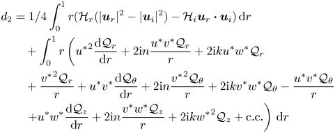 \begin{align} d_2&=1/4\int^1_0r(\mathcal{H}_r(|\boldsymbol{u}_r|^2-|\boldsymbol{u}_i|^2)-\mathcal{H}_i\boldsymbol{u}_r\boldsymbol{\cdot}\boldsymbol{u}_i)\,\textrm{d}r\nonumber\\ &\quad +\int^1_0 r\left({u^*}^2\frac{\textrm{d}\mathcal{Q}_r}{\textrm{d}r}+2\textrm{i}n\frac{u^*v^*\mathcal{Q}_r}{r}+2\textrm{i}ku^*w^*\mathcal{Q}_r \right.\nonumber\\ &\quad +\frac{{v^*}^2\mathcal{Q}_r}{r}+u^*v^*\frac{\textrm{d}\mathcal{Q}_{\theta}}{\textrm{d}r}+2\textrm{i}n\frac{{v^*}^2\mathcal{Q}_{\theta}}{r}+2\textrm{i}kv^*w^*\mathcal{Q}_{\theta}-\frac{u^*v^*\mathcal{Q}_{\theta}}{r}\nonumber\\ &\left. \quad+u^*w^*\frac{\textrm{d}\mathcal{Q}_z}{\textrm{d}r}+2\textrm{i}n\frac{v^*w^*\mathcal{Q}_z}{r}+2\textrm{i}k{w^*}^2\mathcal{Q}_z+\textrm{c.c.}\right)\,\textrm{d}r \end{align}
is a non-zero constant, ( $u^*$, $v^*$, $w^*$) is the complex conjugate of $\boldsymbol {u}$ and $(\mathcal {Q}_r,\mathcal {Q}_{\theta },\mathcal {Q}_z)$ are the three components of $\boldsymbol {\mathcal {Q}}$. Hence $c_1^2=c_2^2$ so that $F$ is 1-D, i.e. $F=F(r)$. The same argument can be applied to subsequent bifurcations (Ding & Kerswell Reference Ding and Kerswell2020) assuming that $d_2$ is generically non-zero at each bifurcation. Since $F$ is always 1-D for $a \ll 1$ as $\alpha \rightarrow 1$, we assume $F$ is 1-D for $\alpha =1$ as well. To summarise, the above shows that energy stability can only design a 1-D baffle.
Appendix B. An unbounded body force and $Re_E \rightarrow \infty$

Here we show that a body force  $\boldsymbol {F}$ can be found which makes $Re_E$ as large as required while maintaining a constant mass flux. A body force determines the laminar flow but does not enter the energy equation for any deviation away from this. Hence the expression for $Re_E$ (2.8) is simplified to
 \begin{equation} \frac{1}{Re_E(\boldsymbol{F})}:= \max_{\boldsymbol{u'}} \frac{-\langle\boldsymbol{u'}\boldsymbol{\cdot}\boldsymbol{u'}\boldsymbol{\cdot}\boldsymbol{\nabla}\boldsymbol{U(\boldsymbol{F})}\rangle} { \langle|\boldsymbol{\nabla}\boldsymbol{u}'|^2\rangle}, \end{equation}
where  $\boldsymbol {F}$ is constrained by the mass flux condition $\left \langle \boldsymbol {U} \boldsymbol {\cdot } \boldsymbol {e}_z \right \rangle ={1}/{2}$. We now construct a sequence of $C^{\infty }$ unidirectional forces, $\boldsymbol {F}:=f_{\varepsilon }(r)/Re\, \boldsymbol {e}_z$, parameterised by a small positive real number $\varepsilon$ and then demonstrate that $Re_E \rightarrow \infty$ as $\varepsilon \rightarrow 0$ where the limiting force is not smooth. The force $f_{\varepsilon }$ is defined as follows:
 \begin{equation} f_{\varepsilon}:=-\frac{1}{r} \frac{\textrm{d}}{\textrm{d}r} \left( r \frac{\textrm{d}W_{\varepsilon}}{\textrm{d}r} \right), \end{equation}
with
 \begin{equation} W_{\varepsilon}(r):= \frac{1}{2}\tanh \left( \frac{1-r}{\varepsilon} \right), \end{equation}
where  $\varepsilon \ll 1$ so there is a boundary layer at $r=1$ ( $W(1)=0$, $\textrm {d}W_{\varepsilon }/\textrm {d}r=O(e^{-2/\varepsilon })$ at $r=0$ and the mass flux condition is satisfied to leading order in $\varepsilon$). The force $f_{\varepsilon }$ is $O(1/\varepsilon ^2)$ in a boundary layer of thickness $O(\varepsilon )$ near the pipe wall and decays exponentially into the interior. Then $1/Re_E$ is the largest eigenvalue $\varLambda (\,f_{\varepsilon })$ of the self-adjoint spectral problem
 \begin{equation} \frac{1}{2}\frac{\textrm{d}W_{\varepsilon}}{\textrm{d}r} \left[ \begin{array}{c} w \\ 0 \\ u \end{array} \right] +\boldsymbol{\nabla} p= \varLambda(\,f_{\varepsilon}) \nabla^2 \boldsymbol{u}, \end{equation}
where  $\boldsymbol {\nabla } \boldsymbol {\cdot } \boldsymbol {u}=0$ and $\boldsymbol {u}=u \boldsymbol {e}_r+v \boldsymbol {e}_{\theta }+w \boldsymbol {e}_z$ is regular at $r=0$ and vanishes at $r=1$.
Since  $W_{\varepsilon }$ is only a function of $r$, this spectral problem can be partitioned into 1-D spectral problems parameterised by an azimuthal wavenumber $m \in \mathbb {N}$ and axial wavenumber $\gamma \in \mathbb {R}$. By inspection, the optimal solution as $\varepsilon \rightarrow 0$ must have a boundary layer of thickness $O(\varepsilon )$ at $r=1$ and either $m=O(1/\varepsilon )$ or $\gamma =O(1/\varepsilon )$ or both with $\varLambda =O(\varepsilon )$. A numerical solution for $\varepsilon =10^{-2}$ and $10^{-3}$ (see figure 11) confirms these scalings and shows that: (a) the optimal is streamwise independent, i.e. $\gamma =0$; and (b) decays exponentially into the interior. These values of $\varepsilon$ are already sufficient to indicate the leading asymptotic behaviour
 \begin{equation} \varLambda(\,f_{\varepsilon})=0.019\varepsilon \end{equation}
with  $m \sim 0.68/\varepsilon$, see figure 11. Clearly, this can be made as small as desired or $Re_E$ as large as desired by choosing $\varepsilon$ sufficiently small (and $\max f_{\varepsilon }=O(1/\varepsilon ^2)$ sufficiently large). Hence there is no maximum $Re_E$ if the force is unconstrained in amplitude.

Figure 11. A contour of  $\varLambda (\,f_{\varepsilon })/\varepsilon$ over $(\varepsilon m ,\varepsilon \gamma )$ showing that maximum $\varLambda (\,f_{\varepsilon })$ is $0.019\varepsilon$ at $(\varepsilon m,\varepsilon \gamma ) = (0.68,0)$ (data for $\varepsilon =0.001$ shown).
For  $Re \lesssim Re_E=O(1/\varepsilon )$, the energy dissipation rate is
 \begin{equation} \frac{1}{Re} \langle |\nabla \boldsymbol{U}|^2 \rangle=\langle FU \rangle = O\left( \frac{1}{\varepsilon^2 Re} \times 1 \times \varepsilon \right) =O \left( \frac{1}{\varepsilon Re} \right)=O(1) \end{equation}
if  $\varepsilon$ is chosen to be just small enough to ensure the energy stability of the forced unidirectional flow $W_{\varepsilon }$. This energy dissipation rate then is more than that associated with the normal turbulent response which is believed to scale as $1/\log (Re)^2$ in units of $U^3/R$. In other words, this strategy of forcing a unidirectional flow is more costly than just letting the flow go turbulent.
Appendix C. The delta function baffle if $\hat {G}$ has a unique minimum

The solution for  $F$ is
 \begin{equation} F=\lim_{\alpha\rightarrow1}a^{1/\alpha}\left[\frac{(-\hat{G})^{\alpha/(\alpha-1)}}{2\int^1_0 r(-\hat{G})^{\alpha/(\alpha-1)}\textrm{d}r}\right]^{1/\alpha}. \end{equation}
Introducing  $q={\alpha }/({\alpha -1})$, we have
 \begin{equation} F=\frac{a}{2}\lim_{q\rightarrow\infty}\frac{(-\hat{G})^{q}}{\int^1_0r(-\hat{G})^q\,\textrm{d}r}. \end{equation}
 Assuming that  $\hat {G}$ has a unique minimum and $\inf \hat {G}<-1$, and we expand $\hat {G}^q$ near the maximal point $r=r^*$ then
 \begin{equation} \hat{G}^q=\exp(q\ln(\hat{G}))\approx\exp(q\ln(-\hat{G}^*)-\gamma q(r-r^*)^2),\quad \gamma=\left.\frac{\hat{G}''}{2\hat{G}}\right|_{r=r^*}>0, \end{equation}
where  $\hat {G}^*=\hat {G}(r^*)$. The integral $\int ^1_0r(-\hat {G})^q\,\textrm {d}r$ is dominated by the principal term when $q\rightarrow \infty$ as follows:
 \begin{equation} \int^1_0r(-\hat{G})^q\,\textrm{d}r\sim (-\hat{G}^*)^q\int^1_0r^*\exp(-\gamma q(r-r^*)^2)\textrm{d}r. \end{equation}
Note that
 \begin{equation} \int^1_0r^*\exp(-\gamma q(r-r^*)^2)\textrm{d}r\sim \frac{1}{\sqrt{\gamma q}},\quad \textrm{so}\quad \int^1_0r(-\hat{G})^q\,\textrm{d}r\sim \frac{(-\hat{G}^*)^q}{\sqrt{\gamma q}}, \end{equation}
thus
 \begin{equation} \int^1_0r(-\hat{G})^q\,\textrm{d}r\sim \frac{(-\hat{G}^*)^q}{\sqrt{\gamma q}}. \end{equation}
Hence, we have
 \begin{equation} F=\frac{a}{2}\lim_{q\rightarrow\infty}\frac{(-\hat{G})^{q}}{\int^1_0r(-\hat{G})^q\,\textrm{d}r}\sim \lim_{q\rightarrow\infty}\frac{a}{2}\sqrt{\gamma q}\left(\frac{\hat{G}}{\hat{G}^*}\right)^q\sim \begin{cases} \dfrac{a}{2}\sqrt{q}, & r=r^*,\\ 0, & r\neq r^*. \end{cases} \end{equation}
This indicates that  $F\sim \delta (r-r^*)$. Because the amplitude of $F$ is constrained by $\left \langle F^{\alpha }\right \rangle ^{1/\alpha }=a$, this indicates that $F$ is
 \begin{equation} F=\frac{a}{2r^*}\delta(r-r^*)\quad \textrm{at}\ \alpha=1. \end{equation}
Appendix D. The Euler–Lagrange equations
Since  $F$ is 1-D, the Lagrangian (3.1) is rewritten as below when the mass flux is fixed,
 \begin{align} \mathscr{L}&=Re+\langle Re{\boldsymbol{u}}'\boldsymbol{\cdot}{\boldsymbol{u}}'\boldsymbol{\cdot}\boldsymbol{\nabla}\boldsymbol{U}\!+\!|\boldsymbol{\nabla}{\boldsymbol{u}}'|^2\!+\!F|{\boldsymbol{u}}'|^2\rangle-\langle p\boldsymbol{\nabla}\boldsymbol{\cdot}{\boldsymbol{u}}'\rangle+\mu_1\left(\left(2\int^1_0 F^{\alpha}r\,\textrm{d}r\right)^{1/\alpha}-a\right)\nonumber\\ &\quad +\mu_2\left(\int^1_0 Wr\,\textrm{d}r-\frac{1}{4}\right) +2\int^1_0W^+\left(\frac{\textrm{d}^2W}{\textrm{d}r^2}+\frac{1}{r}\frac{\textrm{d}W}{\textrm{d}r}+c-FW\right)r\,\textrm{d}r\nonumber\\ &\quad +2\int^1_0\mu_3(F-b^2)\textrm{d}r, \end{align}
where  $\boldsymbol {U}=W(r)\boldsymbol {e}_z$. The Euler–Lagrange equations are
 \begin{gather} \frac{\delta \mathscr{L}}{\delta\boldsymbol{u}'}=-Re(\boldsymbol{\nabla}\boldsymbol{U}+\boldsymbol{\nabla}\boldsymbol{U}^{\texttt{T}})\boldsymbol{\cdot}\boldsymbol{u}'+2\nabla^2\boldsymbol{u}'-2F\boldsymbol{u}'-\boldsymbol{\nabla}p=0, \end{gather}
 \begin{gather} \frac{\delta \mathscr{L}}{\delta p}=\boldsymbol{\nabla}\boldsymbol{\cdot}\boldsymbol{u}'=0, \end{gather}
 \begin{gather} \frac{\delta \mathscr{L}}{\delta W}=-2Re\left(\frac{\textrm{d}\overline{u'w'}}{\textrm{d}r}+\frac{\overline{u'w'}}{r}\right)+2\left(\frac{\textrm{d}^2W^+}{\textrm{d}r^2}+\frac{1}{r}\frac{\textrm{d}W^+}{\textrm{d}r}\right)-2FW^++\mu_2=0, \end{gather}
 \begin{gather} \frac{\delta \mathscr{L}}{\delta F}=2\overline{{u'}^2+{v'}^2+{w'}^2}+2a^{1-\alpha}\mu_1F^{\alpha-1}-2W^+W+2\mu_3=0, \end{gather}
 \begin{gather} \frac{\delta \mathscr{L}}{\delta\mu_1}=\left(2\int^1_0 F^{\alpha}r\,\textrm{d}r\right)^{1/\alpha}-a=0, \end{gather}
 \begin{gather} \frac{\delta \mathscr{L}}{\delta W^+}=\frac{\textrm{d}^2W}{\textrm{d}r^2}+\frac{1}{r}\frac{\textrm{d}W}{\textrm{d}r}-FW+c=0, \end{gather}
 \begin{gather} \frac{\delta \mathscr{L}}{\delta Re}=\langle\boldsymbol{u'}\boldsymbol{\cdot}\boldsymbol{u'}\boldsymbol{\cdot}\boldsymbol{\nabla}\boldsymbol{U}\rangle+1=0, \end{gather}
 \begin{gather} \delta\mathscr{L}/\delta \mu_2=\int^1_0 Wr\,\textrm{d}r-\frac{1}{4}=0, \end{gather}
 \begin{gather} \delta\mathscr{L}/\delta c=\int^1_0W^+r\,\textrm{d}r=0, \end{gather}
where  $\bar {(\bullet )}=\int ^{2{\rm \pi} }_0\int ^L_0 (\bullet )\,\textrm {d}\theta \,\textrm {d}z/{2{\rm \pi} L}$ is the average on a cylindrical surface. Here, we should enforce $F\ge 0$. To realise this, we will set $2\overline {{u'}^2+{v'}^2\!+\!{w'}^2}-2W^+W\!+\!2\mu _3=0$ when $F\!<\!0$ occurs. This indicates that $\mu _3$ is to adjust the value of the $2\overline {{u'}^2+{v'}^2+{w'}^2}-2W^+W$.
D.1. One critical mode only
When there is only one critical mode, we write the mode as
 \begin{align} [{u_1}',{v_1}',{w_1}',{p_1}']=[u_{1r}+iu_{1i},v_{1r}+iv_{1i},w_{1r}+iw_{1i},p_{1r}+ip_{1i}](r)\exp(\textrm{i}kz+\textrm{i}\theta)+\textrm{c.c.} \end{align}
We also fix the phase of this mode by setting  $(u_{1r},v_{1r},w_{1r},p_{1r})^{\textrm {T}}\perp (u_{1i},v_{1i},w_{1i},p_{1i})^{\textrm {T}}$ such that the Euler–Lagrange equations admit a unique solution.
A condition for the wavenumber  $k$ should be added such that our algorithm can find the optimal $k$ automatically,
 \begin{equation} \frac{\delta \mathscr{L}}{\delta k}=2k\int^1_0(u_{1r}^2+u_{1i}^2+v_{1r}^2+v_{1i}^2+w_{1r}^2+w_{1i}^2) r\,\textrm{d}r -\int^1_0(p_{1i}w_{1r}-p_{1r}w_{1i})r\,\textrm{d}r=0. \end{equation}
D.2. Degeneracy of the eigenvalue problem
When  $a$ is above a critical value (e.g. $a=0.96$ for $\alpha =2$), other modes, which are unstable, appear and the eigenvalue problem of the energy stability becomes degenerate. When this occurs, we have to pin all the critical modes such that no unstable modes arise from the energy stability. The ensuing variational problem is reminiscent of, but distinct from, the ‘upper bound’ problem of finding the maximal friction factor possible in turbulent pipe flow (Plasting & Kerswell Reference Plasting and Kerswell2005). In the ‘upper bound’ problem, the so-called ‘spectral constraint’ – a modified version of the energy stability – should be always satisfied, such that a bound on the viscous dissipation can be delivered. However, the ‘upper bound’ problem wishes to maximise the viscous dissipation in a turbulent pipe flow, while we aim to stabilise the flow by a baffle such that the state is always laminar here.
For  $n>1$, we find $k=0$ numerically (see figure 12), and therefore the perturbation can be written as
 \begin{gather} u'={u_1}'+\sum_{n=2}^N u_{n}(r)\cos(n\theta), \end{gather}
 \begin{gather} v'={v_1}'+\sum_{n=2}^N v_{n}(r)\sin(n\theta), \end{gather}
 \begin{gather} w'={w_1}'+\sum_{n=2}^N w_{n}(r)\cos(n\theta), \end{gather}
 \begin{gather} p'={p_1}'+\sum_{n=2}^N p_{n}(r)\cos(n\theta). \end{gather}
Figure 12. The eigenvalues  $\lambda$ of the energy stability versus the wavenumber $k$ for $(a)$
$(a)$ $a=1$ and $(b)$
$(b)$ $a=5$. The norm index $\alpha =2$. The red-solid line is for $n=1$; the blue-dashed line is for $n=2$ and the green-dash-dot line is for $n=3$. The rest of the non-critical modes are not shown. Clearly, for all $n\neq 1$, the critical modes are streamwise homogeneous, i.e. $k=0$.
Hence, the first critical mode  $n=1$, $k\neq 0$ satisfies the following energy stability equation:
 \begin{gather} -Re\frac{\textrm{d}W}{\textrm{d}r}w_{1r}-\frac{\partial}{\partial r}p_{1r}+2\mathcal{L}u_{1r}-2\frac{u_{1r}}{r^2}+4n\frac{v_{1i}}{r^2}-2Fu_{1r}=0, \end{gather}
 \begin{gather} \frac{n}{r}p_{1i}+2\mathcal{L}v_{1r}-2\frac{v_{1r}}{r^2}-4n\frac{u_{1i}}{r^2}-2Fv_{1r}=0, \end{gather}
 \begin{gather} -Re\frac{\textrm{d}W}{\textrm{d}r}u_{1r}+kp_{1i}+2\mathcal{L}w_{1r}-2Fw_{1r}=0, \end{gather}
 \begin{gather} -Re\frac{\textrm{d}W}{\textrm{d}r}w_{1i}-\frac{\partial}{\partial r}p_{1i}+2\mathcal{L}u_{1i}-2\frac{u_{1i}}{r^2}-4n\frac{v_{1r}}{r^2}-2Fu_{1i}=0, \end{gather}
 \begin{gather} -\frac{n}{r}p_{1r}+2\mathcal{L}v_{1i}-2\frac{v_{1i}}{r^2}+4n\frac{u_{1r}}{r^2}-2Fv_{1i}=0, \end{gather}
 \begin{gather} -Re\frac{\textrm{d}W}{\textrm{d}r}u_{1i}-kq_{1r}+2\mathcal{L}w_{1i}-2Fw_{1i}=0, \end{gather}
 \begin{gather} \frac{\textrm{d}u_{1r}}{\textrm{d}r}+\frac{u_{1r}}{r}-\frac{nv_{1i}}{r}-kw_{1i}=0, \end{gather}
 \begin{gather} \frac{\textrm{d}u_{1i}}{\textrm{d}r}+\frac{u_{1i}}{r}+\frac{nv_{1r}}{r}+kw_{1r}=0, \end{gather}
where
 \begin{equation} \mathcal{L}=\frac{\partial^2}{\partial r^2}+\frac{1}{r}\frac{\partial}{\partial r}-\frac{n^2}{r^2}-k^2. \end{equation}
 The boundary conditions for the first mode at  $r=0$ are
 \begin{equation} \frac{\textrm{d}u_{1r}}{\textrm{d}r}=\frac{\textrm{d}u_{1i}}{\textrm{d}r}=\frac{\textrm{d}v_{1r}}{\textrm{d}r}=\frac{dv_{1i}}{\textrm{d}r}=w_{1r}=w_{1i}=p_{1r}=p_{1i}=0. \end{equation}
 For  $n\ge 2$, the energy stability equation is
 \begin{gather} -Re\frac{\textrm{d}W}{\textrm{d}r}w_{n}-\frac{\partial}{\partial r}p_{n}+2\mathcal{L}u_{n}-2\frac{u_{n}}{r^2}-4n\frac{v_{n}}{r^2}-2Fu_n=0, \end{gather}
 \begin{gather} \frac{n}{r}p_{n}+2\mathcal{L}v_{n}-2\frac{v_{n}}{r^2}-\frac{4n}{r^2}u_{n}-2Fv_n=0, \end{gather}
 \begin{gather} -Re\frac{\textrm{d}W}{\textrm{d}r}u_{n}+2\mathcal{L}w_{n}-2Fw_n=0, \end{gather}
 \begin{gather} \frac{\textrm{d}u_{n}}{\textrm{d}r}+\frac{u_{n}}{r}+\frac{nv_{n}}{r}=0, \end{gather}
where
 \begin{equation} \mathcal{L}=\frac{\partial^2}{\partial r^2}+\frac{1}{r}\frac{\partial}{\partial r}-\frac{n^2}{r^2}. \end{equation}
 The boundary conditions for the other modes ( $n\ge 2$) at $r=0$ are
 \begin{equation} u_n=v_n=w_n=p_n=0. \end{equation}
 The adjoint field  $W^+$ satisfies
 \begin{align} &-4Re\left(\frac{\textrm{d}(u_{1r}w_{1r}+u_{1i}w_{1i})}{\textrm{d}r}+\frac{u_{1r}w_{1r}+u_{1i}w_{1i}}{r}\right) -\sum_{n=2}^N\,Re\left(\frac{\textrm{d}u_{n}w_{n}}{\textrm{d}r}+\frac{u_{n}w_{n}}{r}\right)\nonumber\\ &\qquad +2\left(\frac{\textrm{d}^2W^+}{\textrm{d}r^2}+\frac{1}{r}\frac{\textrm{d}W^+}{\textrm{d}r}\right)-2FW^++\mu_2=0. \end{align}
Equation (D 5) for baffle shape function  $F$ is restated as
 \begin{align} &4(u_{1r}^2+u_{1i}^2+v_{1r}^2+v_{1i}^2+w_{1r}^2+w_{1i}^2)+\sum_{n=2}^Nu_n^2+v_n^2+w_n^2\nonumber\\ &\quad +2a^{1-\alpha}\mu_1F^{\alpha-1}-2W^+W+2\mu_3=0. \end{align}
The equation to normalise the Reynolds stress (D 8) becomes
 \begin{equation} 4\int^1_0\frac{\textrm{d}W}{\textrm{d}r}(u_{1r}w_{1r}+u_{1i}w_{1i})r\,\textrm{d}r+\sum_{n=2}^N\int^1_0\frac{\textrm{d}W}{\textrm{d}r}(u_{n}w_{n})r\,\textrm{d}r+1=0. \end{equation}
We follow Plasting & Kerswell (Reference Plasting and Kerswell2005) and use a Newton method with parametric continuation to solve the optimisation problem. Once a new mode becomes unstable, we need to include this new mode in the Newton code. If a mode damps to zero as  $a$ increases, we drop this mode from our computation. The Chebyshev collocation method is used to solve the problem numerically. Once the relative error $|\delta \boldsymbol {x}/\boldsymbol {x}|$ ( $\boldsymbol {x}$ refers to the solution of the Euler–Lagrange equations) is below $10^{-8}$, we terminate the Newton's iteration. The energy stability is then checked when the solution is converged (see figure 12).


 Open access