


1. Introduction
When a vessel containing liquid undergoes periodic vertical oscillations, the free liquid surface may be parametrically destabilized with excitation of standing waves depending on the combination of forcing amplitude and frequency. The threshold at which the instability appears is a function of the corresponding mode dissipation and the excited wavelength is generally specified by the wave whose natural frequency is half that of the parametric excitation, as first noticed by Faraday (Reference Faraday1831), who observed experimentally that the resonance was typically of a subharmonic nature. This observation was later confirmed by Rayleigh (Reference Rayleigh1883a,Reference Rayleighb), in contrast with Matthiessen (Reference Matthiessen1868, Reference Matthiessen1870), who observed synchronous vibrations of the free surface with the vertical shaking. The pioneering work of Benjamin & Ursell (Reference Benjamin and Ursell1954) gave momentum to the theoretical investigations of the Faraday instability. Using first principles, Benjamin & Ursell (Reference Benjamin and Ursell1954) determined the linear stability of the flat free surface of an ideal fluid within a vertically vibrating container displaying a sliding contact line which intersects orthogonally the container sidewalls. The stability is governed by a system of uncoupled Mathieu equations, which predict that standing capillary–gravity waves appear inside the so-called Faraday tongues in the driving frequency–amplitude space, with the wave response that can be subharmonic, harmonic or superharmonic, hence reconciling previous observations.
The effect of viscous dissipation, taken to be linear and sufficiently small, was initially introduced heuristically (Lamb Reference Lamb1932; Landau & Lifshitz Reference Landau and Lifshitz1959) in the inviscid solution, resulting in a semiphenomenological damped Mathieu equation, which was later proved by the viscous linear Floquet theory of Kumar & Tuckerman (Reference Kumar and Tuckerman1994) to be inaccurate, even at small viscosities. An improved version of the damped Mathieu equation, accounting in a more rigorous manner for the dissipation taking place in the free surface and bottom boundary layer, was proposed by Müller et al. (Reference Müller, Wittmer, Wagner, Albers and Knorr1997), who also noticed in their experiments that the fluid depth can affect the Faraday threshold, with harmonic responses most likely to be triggered for thin fluid layers. The viscous theory of Kumar & Tuckerman (Reference Kumar and Tuckerman1994), formulated for a horizontally infinite domain, was found to give good agreement with the small-depth large-aspect-ratio experiments of Edwards & Fauve (Reference Edwards and Fauve1994), where the influence of lateral walls was negligible. If indeed, at large excitation frequencies, where the excited wavelength is much smaller than the container characteristic length, the accessible range of spatial wavenumber is nearly continuous, in the low-frequency regime of single-mode excitation the mode quantization owing to the container sidewall becomes a dominant factor, leading to a discrete spectrum of resonances.
A generalization of the viscous Floquet theory to spatially finite systems can be readily obtained by analogy with the inviscid formulation of Benjamin & Ursell (Reference Benjamin and Ursell1954), as Batson, Zoueshtiagh & Narayanan (Reference Batson, Zoueshtiagh and Narayanan2013) recently proposed. It has, however, intrinsic limitations as it relies on ideal lateral wall conditions, i.e. the unperturbed free surface is assumed to be flat, the contact line is ideally free to slip with a constant zero slope and the stress-free sidewall boundary condition is required for mathematical tractability, since it allows for convenient Bessel-eigenfunctions representation. With the noticeable exception of the sophisticated experiments by Batson et al. (Reference Batson, Zoueshtiagh and Narayanan2013) and Ward, Zoueshtiagh & Narayanan (Reference Ward, Zoueshtiagh and Narayanan2019) using a gliding liquid coating, these assumptions, by overlooking the contact line dynamics, lead in most experimental cases to a considerable underestimation of the actual overall dissipation, resulting in many cases in an inaccurate prediction of the linear Faraday thresholds in small-container experiments (Benjamin & Ursell Reference Benjamin and Ursell1954; Dodge, Kana & Abramson Reference Dodge, Kana and Abramson1965; Ciliberto & Gollub Reference Ciliberto and Gollub1985; Henderson & Miles Reference Henderson and Miles1990; Tipton & Mullin Reference Tipton and Mullin2004; Das & Hopfinger Reference Das and Hopfinger2008). The complexity of the region in the neighbourhood of a moving contact line, where molecular, boundary layer and macroscopic scales are intrinsically connected, is indeed of extreme importance and, despite the significant efforts devoted by several authors to its theoretical understanding (Case & Parkinson Reference Case and Parkinson1957; Keulegan Reference Keulegan1959; Miles Reference Miles1967; Davis Reference Davis1974; Hocking Reference Hocking1987; Miles Reference Miles1990, Reference Miles1991; Cocciaro, Faetti & Nobili Reference Cocciaro, Faetti and Nobili1991; Cocciaro, Faetti & Festa Reference Cocciaro, Faetti and Festa1993; Ting & Perlin Reference Ting and Perlin1995; Perlin & Schultz Reference Perlin and Schultz2000; Jiang, Perlin & Schultz Reference Jiang, Perlin and Schultz2004), the comparison with moving-contact-line experiments, due to unavoidable sources of uncertainty in the meniscus dynamics, remained mostly qualitative, rather than quantitative, requiring often the use of fitting parameters, e.g. a larger effective fluid viscosity (Henderson & Miles Reference Henderson and Miles1990).
A natural means to get rid of the extra dissipation produced by the contact line dynamics is to simply pin the free surface at the edge of the sidewall, i.e. the container is filled to the brim. In such a condition, the overall dissipation is ruled by that occurring in the fluid bulk and in the Stokes boundary layers at the bottom and at the solid lateral walls, where the fluid obeys the classic no-slip boundary condition, relaxing the stress-singularity at the contact line (Navier Reference Navier1823; Huh & Scriven Reference Huh and Scriven1971; Davis Reference Davis1974; Miles Reference Miles1990; Ting & Perlin Reference Ting and Perlin1995; Lauga, Brenner & Stone Reference Lauga, Brenner and Stone2007). Even in the inviscid context, the problem of a pinned contact line boundary condition is well-posed, as shown by the seminal works of Benjamin & Scott (Reference Benjamin and Scott1979) and Graham-Eagle (Reference Graham-Eagle1983), who first solved the resulting dispersion relation for inviscid capillary–gravity waves with a free surface pinned at the container brim using a variational approach and a suitable Lagrange multiplier. Since then, several semianalytical techniques, often combining an inviscid solution with boundary layer approximations and asymptotic expansions accounting for viscous dissipation, have therefore been developed to solve the pinned contact line problem, for example in cylindrical containers (Henderson & Miles Reference Henderson and Miles1994; Martel, Nicolas & Vega Reference Martel, Nicolas and Vega1998; Miles & Henderson Reference Miles and Henderson1998; Nicolás Reference Nicolás2002, Reference Nicolás2005; Kidambi Reference Kidambi2009). The resulting predictions of natural frequencies and damping coefficients of these capillary–gravity waves, in contradistinction with the case of a moving contact line, showed a remarkable agreement with experimental measurements (Henderson & Miles Reference Henderson and Miles1994; Howell et al. Reference Howell, Buhrow, Heath, McKenna, Hwang and Schatz2000).
Within the framework of the Faraday instabilities, this pinned contact line condition can be reached by carefully filling up the vessel up to the brimful condition, as done by Douady (Reference Douady1990) and Edwards & Fauve (Reference Edwards and Fauve1994), among others. Nevertheless, as noticed by Bechhoefer et al. (Reference Bechhoefer, Ego, Manneville and Johnson1995), these delicate experimental conditions are not always perfectly achieved, leading to the presence of a minute meniscus. As mentioned for instance by Douady (Reference Douady1990), the meniscus cannot remain steady upon the oscillating vertical motion of the vessel, which results in the emission of travelling waves from the sidewall to the interior. Irrespective of the pinned or free-edge nature of the contact line, these so-called meniscus waves are synchronized with the excitation frequency. They are not generated by the parametric resonance, but rather by the modulation of the gravitational acceleration resulting in an oscillating capillary length. They do not need to overcome a minimal threshold in forcing amplitude to appear, are therefore observable in the whole driving frequency-amplitude space and are well described by a purely linear response, i.e. at sufficiently small forcing amplitude, the meniscus-wave amplitude is proportional to the external forcing amplitude. As stated by Douady (Reference Douady1990), edge waves constitute a new time-dependent base state on which the instability of parametric waves may develop, possibly blurring the experimental detection of the true Faraday thresholds. This has led researchers to attempt to suppress edge waves by selecting large-aspect-ratio containers where sidewall effects are negligible, using sloping sides or shelf conditions to mitigate edge waves by impedance matching (Bechhoefer et al. Reference Bechhoefer, Ego, Manneville and Johnson1995), or employing highly viscous fluid which damp out these waves (Douady Reference Douady1990; Bechhoefer et al. Reference Bechhoefer, Ego, Manneville and Johnson1995).
With interests in pattern formation, pure meniscus-wave-patterns were investigated for themselves by Torres et al. (Reference Torres, Pastor, Jiménez and Espinosa1995), while complex patterns originating by the coupling of meniscus and Faraday waves were recently described by Shao et al. (Reference Shao, Gabbard, Bostwick and Saylor2021a,Reference Shao, Wilson, Saylor and Bostwickb) for small circular cylinder experiments. A discussion about harmonic Faraday waves disturbed by harmonic meniscus waves (MW) is also outlined in Batson et al. (Reference Batson, Zoueshtiagh and Narayanan2013), where the presence of edge waves in a small circular cylinder bilayer experiment leads to an imperfect bifurcation diagram, also referred to as a tailing effect by Virnig, Berman & Sethna (Reference Virnig, Berman and Sethna1988), who analysed subharmonic responses only. Interestingly, in some cases, e.g. liquid-based biosensors for DNA detection (Picard & Davoust Reference Picard and Davoust2007), tunable small-amplitude stationary waves as MW are actually desired and preferred to saturated larger-amplitude Faraday waves. In such applications, a starting brimful condition, having a contact line fixed at the brim, is ideal since the effective static contact angle at the wall and hence the size and shape of the static meniscus, which will emit edge waves under vertical excitations, can be adjusted simply by increasing or decreasing the bulk volume (nearly brimful condition).
Although the non-conventional eigenvalue problem for natural frequencies and damping coefficients of pinned-contact-line capillary–gravity waves was tackled by several authors mentioned above and in spite of the vastness of literature focused on Faraday waves, there is lack of a comprehensive theoretical framework for the investigation of such a configuration within the context of Faraday instability. An important exception is the work of Kidambi (Reference Kidambi2013). Assuming inviscid Faraday waves in a brimful cylinder with an ideally flat static free surface, Kidambi represented the problem using appropriate modal solutions followed by a projection on a test function space and showed that the pinned contact line condition resulted in an infinite system of coupled Mathieu equations, unlike the classic case of an ideal moving contact line (Benjamin & Ursell Reference Benjamin and Ursell1954). Nevertheless, viscosity, crucial for an accurate prediction of the Faraday threshold, was not included in the analysis, nor was the presence of a static meniscus and its consequent emission of MW. Some attempts to include meniscus modifications to the Faraday thresholds have been made by several authors by including periodic inhomogeneities (Ito, Tsuji & Kukita Reference Ito, Tsuji and Kukita1999; Tipton Reference Tipton2003) and ad hoc phenomenological terms (Lam & Caps Reference Lam and Caps2011) to an ad hoc damped Mathieu equation.
The purpose of this work is to take one more step in the direction undertaken by Kidambi (Reference Kidambi2013), by rigorously accounting for (i) viscous damping, (ii) a pinned contact line and (iii) the presence of a static meniscus at rest. As mentioned above, a contact angle different from  $90^{\circ }$ not only results in a static meniscus, but also induces the emission of meniscus waves as the static meniscus shape is no longer a solution of the forced problem, even below the Faraday threshold. A Floquet-inspired linear theory à la Kumar & Tuckerman (Reference Kumar and Tuckerman1994) cannot be pursued, as perturbations develop around an oscillating base-flow. In contrast, we propose to use the weakly nonlinear (WNL) approach to approximate the linear Faraday bifurcations, although it is expected to involve cumbersome calculations.
Weakly nonlinear analyses (Miles Reference Miles1984; Meron & Procaccia Reference Meron and Procaccia1986; Nayfeh Reference Nayfeh1987; Nagata Reference Nagata1989; Douady Reference Douady1990; Henderson & Miles Reference Henderson and Miles1990; Milner Reference Milner1991; Zhang & Vinals Reference Zhang and Vinals1997; Chen & Vinals Reference Chen and Vinals1999; Jian & Xuequan Reference Jian and Xuequan2005; Skeldon & Guidoboni Reference Skeldon and Guidoboni2007; Rajchenbach & Clamond Reference Rajchenbach and Clamond2015) have indeed been widely used in the context of Faraday instabilities to study the wave amplitude saturation via super and subcritical bifurcations, as well as to investigate pattern and quasipattern formation (Stuart & Fauve Reference Stuart and Fauve1993; Edwards & Fauve Reference Edwards and Fauve1994) or spatiotemporal chaos (Ciliberto & Gollub Reference Ciliberto and Gollub1985; Gluckman et al. Reference Gluckman, Marcq, Bridger and Gollub1993), arising when two modes with nearly the same frequency share the same unstable region in the parameter space and strongly interact. In contradistinction with these previous studies, the presence of a static meniscus calls for a WNL approach not only to estimate the wave amplitude saturation in the WNL regime, but also to predict the Faraday threshold. Hence, with regard to cylindrical straight sidewalls and sharp-edged containers, as the one considered by Shao et al. (Reference Shao, Wilson, Saylor and Bostwick2021b), we derive a WNL model capable of simultaneously accounting of viscous dissipation, static meniscus and MW, thus allowing us to predict their influence on the linear Faraday threshold for standing capillary–gravity waves with pinned contact line as well as their saturation to finite amplitude. Following the recent experimental evidence of Shao et al. (Reference Shao, Wilson, Saylor and Bostwick2021b), we focus on single-mode subharmonic resonances. To this end, the full system of equations governing the fluid motion is solved asymptotically by means of the method of multiple time scales, involving a series of linear problems, which are solved numerically. The theoretical model results in a final amplitude equation for the wave amplitude,  $B$, whose form corresponds to that derived by Douady (Reference Douady1990) using symmetry arguments solely and keeping only low-order terms,
 \begin{equation} \frac{{\rm d}B}{{\rm d}t}={-}\left(\sigma+\text{i}\varLambda/2\right)B+\zeta FB^*+\chi|B|^2B. \end{equation}
This equation correctly predicts the existence of a so-called subharmonic Faraday tongue in the forcing frequency-amplitude (i.e. the  $\varOmega _d$– $F_d$) plane. Within the tongue the forced response driven at $\varOmega _d$ is linearly unstable and a solution oscillating $\omega$ (which is sufficiently close to $\varOmega _d/2$) emerges. The form of (1.1) is indeed valid whatever the shape of the static surface, mode structure and the boundary condition are, but the normal form coefficients, which account for the effect of the static contact angle and which are complex values owing to the presence of viscosity, are here formally determined in closed form from first principles and computed numerically.
The paper is organized as follows. In § 2 the flow configuration and governing equations are introduced, while the numerical methods and tools employed in the work are presented in § 3. In § 4 we formulate a linear eigenvalue problem for the damping and natural frequency of viscous capillary–gravity waves with pinned contact line, whose numerical solution is compared with several previous experiments and theories in Appendix A. The WNL model for subharmonic Faraday resonances is formalized in § 5. A vis-à-vis comparison with recent experiments by Shao et al. (Reference Shao, Wilson, Saylor and Bostwick2021b) with a pure brimful configuration are discussed before moving to a systematic investigation of meniscus effects. Lastly, for validation purposes, in § 6 the modified bifurcation diagram presented in § 5 is compared for a specific case, i.e. pure axisymmetric dynamics, with fully nonlinear direct numerical simulations (DNS). Final comments and conclusions are outlined in § 7.
2. Flow configuration and governing equations
We consider a cylindrical vessel of radius  $R$ and filled to a depth $h$ with a liquid of density $\rho$ and dynamic viscosity $\mu$ (see figure 1). The vessel undergoes a vertical periodic acceleration $F_d=A_d\varOmega _d^2$, where $A_d$ and $\varOmega _d=2{\rm \pi} f_d$ are the driving amplitude and angular frequency, respectively. In a non-inertial reference frame, the fluid experiences a vertical acceleration due to the unsteady apparent gravitational acceleration $g_{app}(t)=g[1-(F_d/g)\cos {\varOmega _d}\,t]$. The viscous fluid motion is thus governed by the incompressible Navier–Stokes equations,
 \begin{equation} \boldsymbol{\nabla}\boldsymbol{\cdot}\boldsymbol{u}=0,\quad \frac{\partial \boldsymbol{u}}{\partial t}+\left(\boldsymbol{u}\boldsymbol{\cdot}\boldsymbol{\nabla}\right)\boldsymbol{u}+\boldsymbol{\nabla} p-\frac{1}{Re}\Delta\boldsymbol{u}={-}\left(1-\frac{F_d}{g}\cos{\varOmega_d\,t}\right)\hat{\boldsymbol{e}}_z, \end{equation}
where  $\boldsymbol {u}(r,\phi,z,t)=\{u_r(r,\phi,z,t),u_{\phi }(r,\phi,z,t),u_z(r,\phi,z,t)\}^{\rm T}$ is the velocity field and $p(r,\phi,z,t)$ is the pressure field. Equations (2.1) are made non-dimensional by using the container's characteristic length $R$, the characteristic velocity $\sqrt {gR}$ and the time scale $\sqrt {R/g}$. The pressure gauge is set to $\rho g R$. Consequently, the Reynolds number is defined as $Re=\rho g^{1/2} R^{3/2}/\mu$ and the term on the right-hand side represents the time modulation of the non-dimensional gravity acceleration. The domains of validity for $r,$
$r,$  $\phi$ and $z$ are, respectively, $r\in [0,1]$, $\phi \in [0,2{\rm \pi} ]$ and $z\in [-h/R,\eta ]$, with $\eta (r,\phi,t)$ the interface coordinate. Then, at $z=\eta$ we impose the kinematic and dynamic boundary conditions,
 \begin{gather}
\frac{\partial\eta}{\partial
t}+{\left.u_r\right|_{\eta}\frac{\partial\eta}{\partial
r}+\frac{\left.u_{\phi}\right|_{\eta}}{r}\frac{\partial\eta}{\partial\phi}-\left.u_z\right|_{\eta}}=0,
\end{gather}
\begin{gather}
\frac{\partial\eta}{\partial
t}+{\left.u_r\right|_{\eta}\frac{\partial\eta}{\partial
r}+\frac{\left.u_{\phi}\right|_{\eta}}{r}\frac{\partial\eta}{\partial\phi}-\left.u_z\right|_{\eta}}=0,
\end{gather} \begin{gather} -\left.p\right|_{\eta}\boldsymbol{n}\left(\eta\right)+\frac{1}{Re}\left.\left(\boldsymbol{\nabla}\boldsymbol{u}+\boldsymbol{\nabla}^{\rm T}\boldsymbol{u}\right)\right|_{\eta}\boldsymbol{\cdot}\boldsymbol{n}\left(\eta\right)=\frac{1}{Bo}\kappa\left(\eta\right)\boldsymbol{n}\left(\eta\right), \end{gather}
where  $\kappa (\eta )$ is the free surface curvature, $\boldsymbol {n}(\eta )$ is unit vector locally normal to the interface and $Bo$ is the Bond number defined as $Bo=\rho gR^2/\gamma$, with $\gamma$ air–liquid surface tension. At the solid bottom, $z=-h/R=-H$ and at the sidewall, $r=1$; we impose the no-slip boundary condition, $\boldsymbol {u}=\boldsymbol {0}$. Lastly, the dynamic pinned (or fixed) contact line condition is enforced as
 \begin{equation} \left.\frac{\partial\eta}{\partial t}\right|_{r=1}=0. \end{equation}
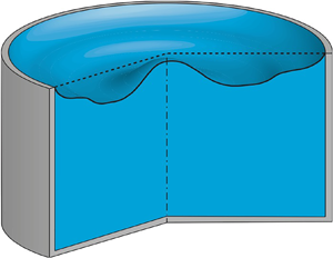
Figure 1. Sketch of a straight sidewalls sharp-edged cylindrical container of radius  $R$ and filled to a depth $h$ with a liquid of density $\rho$ and dynamic viscosity $\mu$. The air–liquid surface tension is denoted by $\gamma$. (a) The free surface, $\eta$, is represented in a generic static configuration characterized by a static contact angle $\theta _s$. (b) Generic dynamic configuration under the external vertical periodic forcing of amplitude $F_d$ and angular frequency $\varOmega _d$. The contact line is pinned and the dynamic angle, oscillating around its static value, $\theta _s$, is denoted by $\theta$. Here $(rz)$–plane is the reference working plane.
3. Numerical methods and tools
Different numerical approaches are adopted in the present paper. The numerical scheme used in the eigenvalue calculation, § 4, and in the WNL analysis, § 5, is a staggered Chebyshev collocation method implemented in MATLAB. The three velocity components are discretized using a Gauss–Lobatto–Chebyshev (GLC) grid, whereas the pressure is staggered on a Gauss–Chebyshev (GC) grid. Accordingly, the momentum equation is collocated at the GLC nodes and the pressure is interpolated from the GC to the GLC grid, while the continuity equation is collocated at the GC nodes and the velocity components are interpolated from the GLC to the GC grid. This results in the classical  $P_N$- $P_{N-2}$ formulation, which automatically suppresses spurious pressure modes in the discretized problem (Viola, Arratia & Gallaire Reference Viola, Arratia and Gallaire2016; Viola & Gallaire Reference Viola and Gallaire2018). A two-dimensional mapping is then used to map the computational space onto the physical space, that has, in general, a curved boundary due to the presence of concave or convex static meniscus. Lastly, the partial derivatives in the computational space are mapped onto the derivatives in the physical space, which depend on the mapping function. For other details see Heinrichs (Reference Heinrichs2004), Canuto et al. (Reference Canuto, Hussaini, Quarteroni and Zang2007), Sommariva (Reference Sommariva2013) and Viola, Brun & Gallaire (Reference Viola, Brun and Gallaire2018).
Mesh convergence was tested for different refinements, starting from a grid size of  $N_r=N_z=20$ up to $N_r=N_z=90$ with a progressive increment of $10$ GLC nodes in both directions. Here $N_r$ and $N_z$ denote the number of radial and axial nodes, respectively. A mesh size of $N_r=N_z=40$ was seen to be sufficient to ensure a convergence of the natural frequencies and damping coefficients (see § A), up to the third digit. However, a mesh $N_r=N_z=80$ was required to ensure the same convergence for the normal form coefficients in the WNL model (see § 5).
The WNL model presented in § 5 involves a third-order asymptotic expansion of the full hydrodynamic system introduced in § 2, that turns out to be very tedious to derive analytically. Therefore, the linearization and expansion procedures have been fully automated using the software Wolfram Mathematica, a powerful tool for symbolic calculus, which has then been integrated within the main MATLAB code. The Mathematica codes are provided in the supplementary material available at https://doi.org/10.1017/jfm.2022.600 as a support to the reader.
In § 6, the results obtained from the WNL analysis are compared and validated for a specific case, i.e. axisymmetric dynamics, with axisymmetric and fully nonlinear DNS, which have been performed using the finite-element software COMSOL Multiphysics v5.6. Further details about the specific DNS setting will be given in § 6.
4. Natural oscillations with pinned contact line and static meniscus
Assuming at first the case with zero external forcing, in this section we provide the framework for the numerical study of the damping coefficients and natural frequencies of viscous capillary–gravity waves with fixed contact line and in the presence of a static meniscus. The flow field  $\boldsymbol {q}(r,\phi,z,t)=\{\boldsymbol {u}(r,\phi,z,t),p(r,\phi,z,t)\}^{\rm T}$ and the interface $\eta (r,\phi,t)$ are decomposed in a static axisymmetric base flow, $\boldsymbol {q}_0(z)=\{\boldsymbol {0},p_0(z)\}^{\rm T}$ and $\eta _0(r)$, and a small perturbation, $\boldsymbol {q}_1(r,\phi,z,t)=\{\boldsymbol {u}_1(r,\phi,z,t),p_1(r,\phi,z,t)\}^{\rm T}$ and $\eta _1(r,\phi,z,t)$, of infinitesimal amplitude $\epsilon$, i.e. $\boldsymbol {q}=\boldsymbol {q}_0+\epsilon \boldsymbol {q}_1$ and $\eta =\eta _0+\epsilon \eta _1$.
4.1. Static meniscus
At rest, the velocity field  $\boldsymbol {u}_0$ is null everywhere and the pressure is hydrostatic, i.e. $p_0=-z$. Therefore, the static configuration is obtained by solving the nonlinear equation associated with the shape of the axisymmetric static meniscus, $\eta _0(r)$,
 \begin{equation} \eta_0-\frac{\kappa\left(\eta_0\right)}{Bo}=0, \end{equation}
with  $\kappa (\eta _0)=(\eta _{0,rr}+\eta _{0,r}(1+\eta _{0,r}^2)/r)(1+\eta _{0,r}^2)^{-3/2}$. At the centreline, $r=0$, the regularity condition $\eta _{0,r}=0$ holds due to axisymmetry. The shape of the meniscus is obtained by imposing the geometric relation at the contact line, $r=1$,
 \begin{equation} \left.\frac{\partial\eta_0}{\partial r}\right|_{r=1}=\cot{\theta_s}, \end{equation}
where  $\theta _s$ is a prescribed static contact angle (see also figure 1a). When $\theta _s$ is set to ${\rm \pi} /2$, then the static interface appears flat.
4.2. Linear eigenvalue problem
Governing equations (2.1) and their boundary conditions (2.2) are then linearized around the static base-flow. It follows that at order  $\epsilon$ the velocity and pressure fields satisfy the Stokes equations
 \begin{equation} \boldsymbol{\nabla}\boldsymbol{\cdot}\boldsymbol{u}_1=0,\quad \frac{\partial \boldsymbol{u}_1}{\partial t}+\boldsymbol{\nabla} p_1-\frac{1}{Re}\Delta\boldsymbol{u}_1=\boldsymbol{0}, \end{equation}
with the linearized kinematic and dynamic free surface boundary conditions (at  $z=\eta _0$)
 \begin{gather} \frac{\partial\eta_1}{\partial t}+{\left.u_{r,1}\right|_{\eta_0}\frac{\partial\eta_0}{\partial r}-\left.u_{z,1}\right|_{\eta_0}}=0, \end{gather}
 \begin{gather} -\left.p_1\right|_{\eta_0}\boldsymbol{n}\left(\eta_0\right)+\eta_1\boldsymbol{n}\left(\eta_0\right)+\frac{1}{Re}\left.\left(\boldsymbol{\nabla}\boldsymbol{u}_1+\boldsymbol{\nabla}^{\rm T}\boldsymbol{u}_1\right)\right|_{\eta_0}\boldsymbol{\cdot}\boldsymbol{n}\left(\eta_0\right)=\frac{1}{Bo}\left.\frac{\partial\kappa\left(\eta\right)}{\partial\eta}\right|_{\eta_0}\eta_1\boldsymbol{n}\left(\eta_0\right), \end{gather}
where  $\boldsymbol {n}(\eta _0)=\{-\eta _{0,r},0,1\}^{\rm T}(1+\eta _{0,r}^2)^{-1/2}$ and
 \begin{align}
\left.\frac{\partial\kappa\left(\eta\right)}{\partial\eta}\right|_{\eta_0}\eta_1
&= \frac{\left(1+\eta_{0,r}^2\right)-3r\eta_{0,r}\eta_{0,rr}}{\left(1+\eta_{0,r}^2\right)^{5/2}}\frac{1}{r}\frac{\partial\eta_1}{\partial
r}+\frac{1}{\left(1+\eta_{0,r}^2\right)^{3/2}}\frac{\partial^2\eta_1}{\partial r^2}\nonumber\\
&\quad +\frac{1}{\left(1+\eta_{0,r}^2\right)^{1/2}}\frac{1}{r^2}\frac{\partial^2\eta_1}{\partial\phi^2}
\end{align}
\begin{align}
\left.\frac{\partial\kappa\left(\eta\right)}{\partial\eta}\right|_{\eta_0}\eta_1
&= \frac{\left(1+\eta_{0,r}^2\right)-3r\eta_{0,r}\eta_{0,rr}}{\left(1+\eta_{0,r}^2\right)^{5/2}}\frac{1}{r}\frac{\partial\eta_1}{\partial
r}+\frac{1}{\left(1+\eta_{0,r}^2\right)^{3/2}}\frac{\partial^2\eta_1}{\partial r^2}\nonumber\\
&\quad +\frac{1}{\left(1+\eta_{0,r}^2\right)^{1/2}}\frac{1}{r^2}\frac{\partial^2\eta_1}{\partial\phi^2}
\end{align}
is the first-order variation of the curvature associated with the small perturbation  $\epsilon \eta _1$. The azimuthal coordinate is denoted by $\phi$. The no-slip boundary condition is imposed at the solid walls, $\boldsymbol {u}_1=\boldsymbol {0}$, while the pinned contact line condition is enforced at the contact line, $z=\eta _0$ and $r=1$,
 \begin{equation} \left.\frac{\partial\eta_1}{\partial t}\right|_{r=1}=0. \end{equation}
Hence, the linear system can be written in compact form as
 \begin{equation} \left({{\boldsymbol{\mathsf{B}}}}\partial_t-{{\boldsymbol{\mathsf{A}}}}\right)\boldsymbol{q}_1=\boldsymbol{0},\quad \text{with}\ {{\boldsymbol{\mathsf{B}}}}=\left( \begin{matrix} I & 0\\ 0 & 0 \end{matrix} \right),\quad {{\boldsymbol{\mathsf{A}}}}=\left( \begin{matrix} Re^{{-}1}\Delta & -\boldsymbol{\nabla}\\ \boldsymbol{\nabla}^{\rm T} & 0 \end{matrix} \right). \end{equation}
We note that the kinematic and the dynamic boundary conditions (4.4) and (4.5) do not explicitly appear in (4.8), but they are imposed as conditions at the interface (Viola & Gallaire Reference Viola and Gallaire2018). More precisely, in the numerical scheme, the kinematic condition governing the state variable  $\eta$ is implemented as an additional equation dynamically coupled with $\boldsymbol {u}_1$ and $p_1$ in (4.8) (this is better clarified in Appendix B of Bongarzone, Viola & Gallaire (Reference Bongarzone, Viola and Gallaire2021b)), whereas the three stress components of the dynamic condition are enforced as standard boundary conditions in the corresponding components of the momentum equation. The solution can be then expanded in terms of normal modes in time and in the azimuthal direction as
 \begin{align} \boldsymbol{q}_1\left(r,\phi,z,t\right)&=\hat{\boldsymbol{q}}_1\left(r,z\right){\rm e}^{\lambda t}{\rm e}^{\text{i}m\phi}+{\rm c.c.}\nonumber\\ &\quad=\left\{\hat{u}_{1r}\left(r,z\right),\hat{u}_{1\phi}\left(r,z\right),\hat{u}_{1z}\left(r,z\right),\hat{p}_1\left(r,z\right)\right\}^{\rm T} {\rm e}^{\lambda t}{\rm e}^{\text{i}m\phi}+{\rm c.c.}, \end{align}
 \begin{align} &\qquad \qquad\eta_1\left(r,\phi,t\right)=\hat{\eta}_1\left(r\right){\rm e}^{\lambda t}{\rm e}^{\text{i}m\phi}+{\rm c.c.} \end{align}
Substituting the normal form (4.9)–(4.10) in system (4.8), we obtain a generalized linear eigenvalue problem,
 \begin{equation} \left(\lambda{{\boldsymbol{\mathsf{B}}}}-{{\boldsymbol{\mathsf{A}}}}_m\right)\hat{\boldsymbol{q}}_1=\boldsymbol{0}, \end{equation}
where the linear operator  ${{\boldsymbol{\mathsf{A}}}}_m$ depends on the azimuthal wavenumber $m$ and $\hat {\boldsymbol {q}}_1$ is the global mode associated with the eigenvalue $\lambda =-\sigma +\text {i}\omega$, with $\sigma$ and $\omega$ the damping coefficient and the natural frequency, respectively, of the $(m,n)$ global mode. Here the indices $(m,n)$ represent the number of nodal circles and nodal diameters, respectively. Owing to the normal mode expansion (4.9), we notice that the operator ${{\boldsymbol{\mathsf{A}}}}_m$ is complex, since $\phi$ derivatives produce $\text {i}m$ terms. A complete expansion of the complex operator can be found in Meliga, Chomaz & Sipp (Reference Meliga, Chomaz and Sipp2009) and Viola & Gallaire (Reference Viola and Gallaire2018).
In order to regularize the problem at the axis, depending on the selected azimuthal wavenumber  $m$, different regularity conditions must be imposed at $r=0$ (Liu & Liu Reference Liu and Liu2012; Viola & Gallaire Reference Viola and Gallaire2018),
 \begin{gather} |m|=0\text{:}\quad \hat{u}_{1r}=\hat{u}_{1\phi}=\frac{\partial\hat{u}_{1z}}{\partial r}=\frac{\partial \hat{p}_1}{\partial r}=0, \end{gather}
 \begin{gather} |m|=1\text{:}\quad \frac{\partial\hat{u}_{1r}}{\partial r}=\frac{\partial\hat{u}_{1\phi}}{\partial r}=\hat{u}_{1z}=\hat{p}_1=0, \end{gather}
 \begin{gather} |m|>0\text{:}\quad \hat{u}_{1r}=\hat{u}_{1\phi}=\hat{u}_{1z}=\hat{p}_1=0. \end{gather}
Lastly, due to the symmetries of the problem, system (4.11) with its boundary conditions is invariant under the
 \begin{equation} \left(\hat{u}_{1r},\hat{u}_{1\phi},\hat{u}_{1z},\hat{p}_1,\hat{\eta}_1,+m,-\sigma+\text{i}\omega\right)\rightarrow\left(\hat{u}_{1r},-\hat{u}_{1\phi},\hat{u}_{1z},\hat{p}_1,\hat{\eta}_1,-m,-\sigma+\text{i}\omega\right), \end{equation}
transformation, so in this section, § 4, we consider only the case with  $m\geqslant 0$. Furthermore, the following relations hold:
 \begin{gather} \left(\hat{\boldsymbol{q}}_1,\hat{\eta}_1,+m,-\sigma+\text{i}\omega\right)\rightarrow\left(\hat{\boldsymbol{q}}_1^*,\hat{\eta}_1^*,-m,-\sigma-\text{i}\omega\right), \end{gather}
 \begin{gather} \left(\hat{\boldsymbol{q}}_1,\hat{\eta}_1,-m,-\sigma+\text{i}\omega\right)\rightarrow\left(\hat{\boldsymbol{q}}_1^*,\hat{\eta}_1^*,+m,-\sigma-\text{i}\omega\right), \end{gather}
(where the star designates the complex conjugate), i.e. the eigenvalues are complex conjugates and all spectra ( $\pm m$) in the $(\sigma,\omega )$-plane are symmetric with respect to the real axis ( $\omega =0$), but the complex conjugates of the corresponding eigenvectors, except for the axisymmetric dynamics ( $m=0$), are not eigenmodes of the same spectrum. The damping coefficients and natural frequencies of viscous capillary–gravity waves with fixed contact line in both the meniscus-free and with-meniscus configuration are thus computed by solving numerically the generalized eigenvalue problem (4.11), as described in § 3.
With regard to the literature survey outlined in table 1, in Appendix A we propose a thorough validation of our numerical tools via comparison with several pre-existing experiments and theoretical/semianalytical predictions focusing on both brimful and nearly brimful circular cylinders.
Table 1. Literature survey on the natural frequencies and damping coefficients of small-amplitude capillary–gravity waves in labscale upright cylindrical containers with pinned contact line and in both meniscus-free and with-meniscus configurations. The present work lies within the conditions highlighted by the shaded frames. The case examined by K13 and S21 will be discussed afterwards in § 5 within the context of subharmonic Faraday waves.

5. Weakly nonlinear model for subharmonic Faraday thresholds with contact angle effects
In this section, the numerical tools presented and validated in § 4 are employed to formalize a WNL model accounting for contact angle effects, i.e. static meniscus and harmonic meniscus capillary waves, on the subharmonic Faraday instability with pinned contact line.
5.1. Presentation
Here, the full system (2.1)–(2.3) is solved through a WNL analysis based on the multiple scale method that is valid in the regime of small perturbations of the static configuration and small external control parameters, namely the driving amplitude and detuning from the parametric resonance. Let us thus introduce the following asymptotic expansion for the flow quantities:
 \begin{gather} \boldsymbol{q}=\left\{\boldsymbol{u},p\right\}^{\rm T}=\boldsymbol{q}_0+\epsilon\boldsymbol{q}_1+\epsilon^2\boldsymbol{q}_2+\epsilon^3\boldsymbol{q}_3+O\left(\epsilon^4\right), \end{gather}
 \begin{gather} \eta=\eta_0+\epsilon\eta_1+\epsilon^2\eta_2+\epsilon^3\eta_3+O\left(\epsilon^4\right). \end{gather}
 In the spirit of the multiple scale technique, we introduce the slow time scale  $T=\epsilon ^2 t$, with $t$ being the fast time scale at which the free surface oscillates. For subharmonic resonances the system is expected to respond with a frequency equal to half the driving frequency. In order to determine the boundaries of the instability tongues, we assume the external forcing angular frequency to be $\varOmega _d=2\omega +\varLambda$, where $\omega$ is the natural frequency associated with the generic $(m,n)$ capillary–gravity wave considered and $\varLambda$ is the detuning parameter. As, by construction, the WNL analysis is valid close to the instability threshold only, we assume a departure from criticality to be of order $\epsilon ^2$. In terms of control parameters, this assumption translates to the following scalings for the external forcing amplitude, $F_d/g$, and detuning $\varLambda$:
 \begin{equation} F_d/g=F=\epsilon^2\hat{F},\quad \varLambda=\epsilon^2\hat{\varLambda}. \end{equation}
It should be noted that the presence of viscosity leads to a damped  $\epsilon$-order solution $\boldsymbol {q}_1$ (as discussed in § 4), whereas standard multiple scale methods apply to marginally stable systems (Nayfeh Reference Nayfeh2008). Nevertheless, as the Reynolds number is typically high enough, the damping coefficient results in a slow damping process over fast wave oscillations (see § 4). In such a regime, a multiple scale analysis can still be applied by postulating that the damping coefficient of the $(m,n)$ wave is of order $\epsilon ^2$, i.e. $\sigma =\epsilon ^2\hat {\sigma }$, therefore the $(m,n)$ eigenvalue reads $\lambda =-\epsilon ^2\hat {\sigma }+\text {i}\omega$. A simple way to account for this second-order departure from neutrality consists in replacing the leading-order operator ${{\boldsymbol{\mathsf{A}}}}_m={{\boldsymbol{\mathsf{A}}}}_m(Re)$ defined in (4.11), for which $\hat {\boldsymbol {q}}_1$ is not neutral, but rather stable, by the shifted operator (Meliga et al. Reference Meliga, Chomaz and Sipp2009), $\tilde {{{\boldsymbol{\mathsf{A}}}}}_m={{\boldsymbol{\mathsf{A}}}}_m+\epsilon ^2{{\boldsymbol{\mathsf{S}}}}_m$, where ${{\boldsymbol{\mathsf{S}}}}_m$ is the shift operator defined as ${{\boldsymbol{\mathsf{S}}}}_m\hat {\boldsymbol {q}}_1=-\hat {\sigma }\hat {\boldsymbol {q}}_1$. The shifted operator $\tilde {{{\boldsymbol{\mathsf{A}}}}}_m$ is characterized by the same spectra of ${{\boldsymbol{\mathsf{A}}}}_m$, except that the $(m,n)$ eigenmode $\hat {\boldsymbol {q}}_1$ associated with $\hat {\sigma }$ is now marginally stable, and hence the WNL formalism can be applied. For a thorough discussion about the formalism of the shift operator see Meliga et al. (Reference Meliga, Chomaz and Sipp2009) and Meliga, Gallaire & Chomaz (Reference Meliga, Gallaire and Chomaz2012). Although a different approach to account for a damped first-order solution was followed by Viola & Gallaire (Reference Viola and Gallaire2018), leading to a different (but equivalent) asymptotic expansion, we use in this paper the shift operator approach.
Finally, substituting the asymptotic expansions and scalings above in the governing equations (2.1)–(2.3) with their boundary conditions, a series of problems at the different orders in  $\epsilon$ are obtained.
As anticipated in § 3, when contact angle effects are included in the analysis, i.e. the initial static interface is not flat, the third-order asymptotic expansion of the full viscous hydrodynamic system introduced in § 2 turns out to be very complex to derive analytically. Particularly tedious is the dynamic boundary condition, as it involves free surface boundary terms, which, within the linearization process, must be flattened at the static interface,  $\eta _0$, as well as the full nonlinear curvature. In order to overcome these practical difficulties, the linearization and expansion procedures have been fully automated using symbolic calculus within the software Wolfram Mathematica, which has been then integrated within the main code implemented in MATLAB. The corresponding Mathematica codes are provided as supplementary material.
5.2. Order  $\epsilon ^0$: static meniscus

At order  $\epsilon ^0$ the system reduces to the nonlinear equation associated with the shape of the axisymmetric static meniscus. The velocity field is null, $\boldsymbol {u}_0=\boldsymbol {0}$ and the pressure is hydrostatic, $p_0=-z$. As described in § 4.1, the static interface, $\eta _0(r)$, is obtained by prescribing a static contact angle, $\theta _s$, which enters through the geometrical relation (4.2) imposed at the contact line.
5.3. Order $\epsilon$: capillary–gravity waves

At leading order in  $\epsilon$ the system is represented by the unsteady Stokes equations (4.3), together with the kinematic and dynamic boundary conditions (4.4)–(4.5), linearized around the static base flow $\boldsymbol {q}_0=\{\boldsymbol {u}_0,p_0\}^{\rm T}=\{\boldsymbol {0},-z\}^{\rm T}$ and $\eta _0$, and subjected to the no-slip boundary condition at the solid walls, regularity conditions at the axis (4.12a)–(4.12c) and to the pinned contact line condition (4.7),
 \begin{equation} \left({{\boldsymbol{\mathsf{B}}}}\partial_t-\tilde{{{\boldsymbol{\mathsf{A}}}}}_m\right)\boldsymbol{q}_1=\boldsymbol{0}. \end{equation}
Within the framework of the Faraday instability, we are interested in a standing waveform of the solution, which can be seen as a result of the balance of two counter-rotating waves. Hence, we look for a first-order solution of the form
 $$\begin{gather} \boldsymbol{q}_1=A_1^+\left(T\right)\hat{\boldsymbol{q}}_1^{A^+} \exp\left({\text{i}\left(\omega t+m\phi\right)}\right)+A_1^-\left(T\right)\hat{\boldsymbol{q}}_1^{A^-} \exp\left({\text{i}\left(\omega t-m\phi\right)}\right)+{\rm c.c.}, \end{gather}$$
 $$\begin{gather}{\eta_1=A_1^+\left(T\right)\hat{\eta}_1^{A^+} \exp\left({\text{i}\left(\omega t+m\phi\right)}\right)+A_1^-\left(T\right)\hat{\eta}_1^{A^-} \exp\left({\text{i}\left(\omega t-m\phi\right)}\right)+{\rm c.c.},} \end{gather}$$
( $\eta _1$ takes the same form) that destabilizes the static configuration. A single azimuthal wavenumber $m$ is considered at a time. In (5.5), $A^+_1$ and $A^-_1$, unknown at this stage of the expansion, are the complex amplitudes of the oscillating mode $\hat {\boldsymbol {q}}_1^{A^+}$ and $\hat {\boldsymbol {q}}_1^{A^-}$, respectively, and they are functions of the slow time scale $T$. The eigensolution of (5.4) has been widely discussed in § 4 for $m\geqslant 0$. We note in addition that the eigenmode for the $-m$ perturbation is similar to that of the $+m$ perturbation; more precisely, it oscillates with the same frequency $\omega$, but it has the opposite pitch and it rotates in the opposite direction.
5.4. Order $\epsilon ^2$: MW, second harmonics and mean-flow corrections

At order  $\epsilon ^2$ we obtain the linearized Stokes equations and boundary conditions applied to $\boldsymbol {q}_2=\{\boldsymbol {u}_2,p_2\}^{\rm T}$ and $\eta _2$,
 \begin{equation} \left({{\boldsymbol{\mathsf{B}}}}\partial_t-\tilde{{{\boldsymbol{\mathsf{A}}}}}_m\right)\boldsymbol{q}_2=\boldsymbol{\mathcal{F}}_2, \end{equation}
and forced by a term  $\boldsymbol {\mathcal {F}}_2$ depending only on zero-, first-order solutions and on the external forcing
 $$\begin{gather} \boldsymbol{\mathcal{F}}_2=|A^+_1|^2\hat{\boldsymbol{\mathcal{F}}}_2^{A^+A^{+^*}}+|A^-_1|^2\hat{\boldsymbol{\mathcal{F}}}_2^{A^-A^{-^*}}+\left(\hat{F}\hat{\boldsymbol{\mathcal{F}}}_2^{\hat{F}} \exp\left({\text{i}\left(2\omega t+\hat{\varLambda}T\right)}\right)+{\rm c.c.}\right)\nonumber\\ +\left(A^{+^2}_1\hat{\boldsymbol{\mathcal{F}}}_2^{A^+A^+} \exp\left({\text{i}\left(2\omega t+2m\phi\right)}\right)+A^{-^2}_1\hat{\boldsymbol{\mathcal{F}}}_2^{A^-A^-} \exp\left({\text{i}\left(2\omega t-2m\phi\right)}\right)+{\rm c.c.}\right)\nonumber\\ +\left(A^+_1A^-_1\hat{\boldsymbol{\mathcal{F}}}_2^{A^+A^-} {\rm e}^{\text{i}2\omega t}+A^+_1A^{-^*}_1\hat{\boldsymbol{\mathcal{F}}}_2^{A^+A^{-^*}} {\rm e}^{\text{i}2m\phi}+{\rm c.c.}\right). \end{gather}$$
All terms contributing to the forcing vector  $\boldsymbol {\mathcal {F}}_2$ were extracted using symbolic calculus in Wolfram Mathematica (see supplementary material). The first-order solution is made of four different contributions of amplitude $A^+_1$, $A^{+^*}_1$, $A^-_1$ and $A^{-^*}_1$, and therefore it generates 10 different second-order forcing terms, $\hat {\boldsymbol {\mathcal {F}}}_2^{ij} \exp ({\text {i}(\omega ^{ij} t+m^{ij}\phi )})$, which exhibit a certain frequency and spatial periodicity, gathered in table 2. The two additional terms, $\hat {\boldsymbol {\mathcal {F}}}_2^{\hat {F}}$, appearing in the forcing expression (5.8), come from the spatially uniform axisymmetric external forcing typical of Faraday waves, whose amplitude was assumed to be of order $\epsilon ^2$.
Table 2. Second-order nonlinear forcing terms gathered by their amplitude dependency, and corresponding azimuthal and temporal periodicity  $(m^{ij},\omega ^{ij})$. Seven terms have been omitted as they are the complex conjugates.

All these forcing terms are non-resonant, as their oscillation frequencies and their spatial symmetries, through the azimuthal wavenumber, differ from those of the leading-order solution (see table 2). Hence no solvability conditions are required at the present order (Meliga et al. Reference Meliga, Chomaz and Sipp2009). We can thus look for a second-order solution as the superposition of the second-order response to the external forcing,  $\hat {\boldsymbol {q}}_2^{\hat {F}}$, and 10 responses $\hat {\boldsymbol {q}}_2^{ij}$ to each single forcing term,
 $$\begin{gather} \boldsymbol{q}_2=|A^+_1|^2\hat{\boldsymbol{q}}_2^{A^+A^{+^*}}+|A^-_1|^2\hat{\boldsymbol{q}}_2^{A^-A^{-^*}}+\left(\hat{F}\hat{\boldsymbol{q}}_2^{\hat{F}} \exp\left({\text{i}\left(2\omega t+\hat{\varLambda}T\right)}\right)+{\rm c.c.}\right)\nonumber\\ +\left(A^{+^2}_1\hat{\boldsymbol{q}}_2^{A^{+^2}} \exp\left({\text{i}\left(2\omega t+2m\phi\right)}\right)+A^{-^2}_1\hat{\boldsymbol{q}}_2^{A^{-^2}} \exp\left({\text{i}\left(2\omega t-2m\phi\right)}\right)+{\rm c.c.}\right)\nonumber\\ +\left(A^+_1A^-_1\hat{\boldsymbol{q}}_2^{A^+A^-} {\rm e}^{\text{i}2\omega t}+A^+_1A^{-^*}_1\hat{\boldsymbol{q}}_2^{A^+A^{-^*}} {\rm e}^{\text{i}2m\phi}+{\rm c.c.}\right), \end{gather}$$
(the same form is assumed for  $\eta _2$) each of which is computed as a solution of a linear forced problem
 \begin{equation} \left(\text{i}\omega^{ij}{{\boldsymbol{\mathsf{B}}}}-\tilde{{{\boldsymbol{\mathsf{A}}}}}_{m^{ij}}\right)\hat{\boldsymbol{q}}_2^{ij}=\hat{\boldsymbol{\mathcal{F}}}_2^{ij}, \end{equation}
with  $m^{ij}$ and $\omega ^{ij}$ for $(i,j)$ from table 2 and which can be inverted (non-singular operator) so long as any of the combinations $(m^{ij},\omega ^{ij})$ is not an eigenvalue (none of them has $m^{ij}=\pm m$). As an example, the $\epsilon$-order eigensurface and some of the various second-order surfaces are shown in figure 2 for three different waves, i.e. $(m,n)=(1,2)$, $(3,2)$ and $(0,2)$. Owing to the symmetries of the system (given in (4.13)), some of the second-order responses corresponding to the generic $(m,n)$ wave have the same solution with opposite azimuthal velocity, therefore in figure 2 we show only the solutions with different surface shapes. Furthermore, as can be deduced from figure 2(m–r), in the axisymmetric case $(0,n)$ all the responses are axisymmetric with zero azimuthal velocity, thus some of the second-order responses share exactly the same solution. In this case, indeed, the second-order solution could be formulated a priori as the sum of three terms only, whose amplitudes are proportional to $\hat {F}$, $A^2_1$ (second harmonic) and $|A_1|^2$ (mean flow correction), respectively.

Figure 2. (a–f) Upper subpanel: real part of the free surface elevation, Re $(\hat {\eta })$ associated with (a) mode $(1,2)$ and with (b–f) some of the corresponding second-order responses for different values of the static contact angle, $\theta _s$. The $\epsilon$-order solution is normalized such that the phase of the interface at the contact line in $\phi =0$ is zero and the corresponding slope is one, i.e. $\hat {\boldsymbol {q}}_1\rightarrow \hat {\boldsymbol {q}}_1 \exp ({-\text {i}\,\text {arctan}[\hat {\eta }_1(r=1,0)]})/(\partial \hat {\eta }_1(r,0)/\partial r|_{r=1})$. Lower subpanel: free surface visualization in terms of absolute value of the real part of the interface slope at $\theta _s=45^{\circ }$. The colourmaps were individually saturated for visualization purposes only. (g–l) Same as (a–f), but for mode $(3,2)$. (m–r) Same as (a–f), but for the axisymmetric mode $(0,2)$. Parameter setting: $R=0.035$ m; $h=0.022$ m; $\rho =997$ kg m $^{-3}$; $\mu =0.001$ kg m $^{-1}$ s $^{-1}$; $\gamma =0.072$ N m $^{-1}$; for which $Bo=166.2$ and $Re=20\,437$, and a static contact angle $\theta _s=45^{\circ }$. The light red boxes highlights the second-order response to the external forcing, i.e. second-order harmonic MW.
Of particular interest is the second-order response to the external forcing, whose interface shape is highlighted by the red boxes in figure 2. With the present scaling, the forcing enters at second order in the  $z$-component of the momentum equation (see (2.1)). If the initial static interface is assumed to be flat ( $\theta _s=90^{\circ }$), then the response $(\hat {\boldsymbol {q}}_2^{\hat {F}},\hat {\eta }_2^{\hat {F}})$, translates into a harmonic hydrostatic pressure modulation only, with a free surface remaining flat, i.e. $\hat {\boldsymbol {u}}_2^{\hat {F}}=\boldsymbol {0}$ and $\hat {\eta }_2^{\hat {F}}=0$, a case classically analysed in the literature. On the other hand, as shown in figure 2(c,i,o), if a static contact angle $\theta _s\ne 90^{\circ }$ is considered, then the $\epsilon ^0$-order static meniscus induces at order $\epsilon ^2$ axisymmetric meniscus capillary waves travelling from the sidewall to the interior and reflected back, which oscillates harmonically with the external forcing and with an amplitude proportional to the external forcing amplitude. In the present WNL analysis, these MW, which appear as concentric ripples (see figure 2c,i,o), as typically observed in experiments (Batson et al. Reference Batson, Zoueshtiagh and Narayanan2013; Shao et al. Reference Shao, Gabbard, Bostwick and Saylor2021a,Reference Shao, Wilson, Saylor and Bostwickb), will couple at third order with the first-order solution and will contribute to modify both the linear stability boundaries associated with the subharmonic Faraday tongues as well as the bifurcation diagram, i.e. wave amplitude saturation to finite amplitude. Furthermore, figure 2 clearly shows that a static contact angle $\theta _s\ne 90$, depending on its value (here only values of $\theta _s<90^{\circ }$ have been considered), modifies not only the damping coefficients and frequencies of the leading-order wave (see also Appendix A), but also its spatial shape and, as consequence, all the associated second-order responses, whose modifications may have a significant influence on the corresponding saturation to a finite amplitude.
5.5. Order $\epsilon ^3$: amplitude equation for standing waves

Lastly, at the  $\epsilon ^3$-order we derive an amplitude equation for standing waves with a pinned contact line accounting for WNL modifications of the subharmonic Faraday threshold due to contact angle effects. The problem at order $\epsilon ^3$ is similar to the one obtained at order $\epsilon ^2$, as it appears as a linear system,
 \begin{equation} \left({{\boldsymbol{\mathsf{B}}}}\partial_t-\tilde{{{\boldsymbol{\mathsf{A}}}}}_m\right)\boldsymbol{q}_3=\boldsymbol{\mathcal{F}}_3, \end{equation}
forced by combinations of the previous-order solutions encompassed in  $\boldsymbol {\mathcal {F}}_3$, that contains several nonlinear terms of various space and time periodicities and which we denote as $\hat {\boldsymbol {\mathcal {F}}}_3^{ij} \exp ({\text {i}(\omega t + m\phi )})$. Since many of these terms are resonant, as standard in multiple scale analysis, in order to avoid secular terms and solve the expansion procedure at the third order, a compatibility condition must be enforced through the Fredholm alternative (Friedrichs Reference Friedrichs2012). Such a compatibility condition imposes the amplitudes $A^+_1$ and $A^-_1$ to obey the following relation:
 \begin{equation} \frac{{\rm d}A^{{\pm}}}{{\rm d}t}={-}\sigma A^{{\pm}} + \zeta FA^{{\mp}^*} {\rm e}^{\text{i}\varLambda t / 2} + \chi_1 |A^{{\pm}}|^2A^{{\pm}} + \chi_2 |A^{{\mp}}|^2A^{{\pm}}, \end{equation}
where the physical time  $t=T/\epsilon ^2$ has been reintroduced and where $\sigma =\epsilon ^2\hat {\sigma }$, $F=F_d/g=\epsilon ^2\hat {F}$ and $\varLambda =\epsilon ^2\hat {\varLambda }$. By considering the expansion $\boldsymbol {q}=\boldsymbol {q}_0+\epsilon A_1\hat {\boldsymbol {q}}_1\dots$, the small parameter $\epsilon$ is eliminated by defining the amplitude $A=\epsilon A_1$, so that everything is recast in terms of actual physical quantities (Bongarzone et al. Reference Bongarzone, Bertsch, Renaud and Gallaire2021a; Bongarzone, Guido & Gallaire Reference Bongarzone, Guido and Gallaire2022). The various coefficients are computed as scalar products between the adjoint global modes and the resonant forcing terms $\hat {\boldsymbol {\mathcal {F}}}_3^{ij}$, whose analytically complex expressions have been extracted from the third-order forcing using the symbolic calculus tools of Wolfram Mathematica. For instance, the complex coefficient $\zeta$ is evaluated as
 \begin{equation} \zeta=\frac{\int_{{V}}\hat{\boldsymbol{u}}_1^{{{\dagger}}^* A^{+}}\boldsymbol{\cdot}\hat{\boldsymbol{\mathcal{F}}}_{3,{NS}}^{\hat{F}A^{-^*}}\,r\,\text{d}r\text{d}z+\int_{\eta_0}\hat{\boldsymbol{u}}_1^{{{\dagger}}^* A^{+}}\boldsymbol{\cdot}\hat{\boldsymbol{\mathcal{F}}}_{3,{D}}^{\hat{F}A^{-^*}}\,r\,\text{d}r +\int_{\eta_0}\xi^{{{\dagger}}^* A^+}\hat{\mathcal{F}}_{3,{K}}^{\hat{F}A^{-^*}}\,r\,\text{d}r}{\int_{{V}}\hat{\boldsymbol{u}}_1^{{{\dagger}}^* A^{+}}\boldsymbol{\cdot}\hat{\boldsymbol{u}}_1^{A^{+}}\,r\,\text{d}r\,\text{d}z+\int_{\eta_0}\xi^{{{\dagger}}^* A^+}\hat{\eta}_1^{A^+}\,r\,\text{d}r}, \end{equation}
where  ${V}$ denotes the fluid bulk domain, the dagger symbol refers to the adjoint eigenmode,
 \begin{equation} \xi = \left[-\frac{\eta_{0,r}}{Re}\left(\frac{\partial \hat{u}_{1z}}{\partial r}+\frac{\partial \hat{u}_{1r}}{\partial z}\right)+\left(-\hat{p}_1+\frac{2}{Re}\frac{\partial \hat{u}_{1z}}{\partial z}\right)\right] \end{equation}
(see also Viola & Gallaire Reference Viola and Gallaire2018) and the subscripts  $_{NS}$, $_{D}$ and $_{K}$ designate the forcing components of $\hat {\boldsymbol {\mathcal {F}}}_3^{\hat {F}A^{-^*}}$ appearing in the $\epsilon ^3$-order Navier–Stokes equations, dynamic boundary condition and kinematic boundary condition, respectively. Analogous expressions hold for $\chi _1$ and $\chi _2$ by replacing $\hat {\boldsymbol {\mathcal {F}}}_3^{\hat {F}A^{-^*}}$ with $\hat {\boldsymbol {\mathcal {F}}}_3^{A^+A^{+^*}A^+}$ and $\hat {\boldsymbol {\mathcal {F}}}_3^{A^-A^{-^*}A^+}$, respectively. We notice that the adjoint eigenvector appearing in (5.13) does not need to be independently calculated. Indeed, Viola & Gallaire (Reference Viola and Gallaire2018) demonstrated that the linear operator ${{\boldsymbol{\mathsf{B}}}}$ and ${{\boldsymbol{\mathsf{A}}}}_m$ (the same applies to the shifted operator $\tilde {{{\boldsymbol{\mathsf{A}}}}}_m$) are self-adjoint, i.e. ${{\boldsymbol{\mathsf{B}}}}^{{\dagger} }={{\boldsymbol{\mathsf{B}}}}$ and ${{\boldsymbol{\mathsf{A}}}}_m^{{\dagger} }={{\boldsymbol{\mathsf{A}}}}_m$, with the adjoint eigenvalue being the complex conjugate of the direct one, $\lambda ^{{\dagger} }=\lambda ^*$. Then, from (4.13), (4.14) and (4.15), it follows that for the couple $(m,-\sigma +\text {i}\omega )$ associated with a direct mode, we have the relation
 \begin{equation} \left(\hat{u}_{1r}^*,-\hat{u}_{1\phi}^*,\hat{u}_{1z}^*,\hat{p}_1^*,\hat{\eta}_1^*\right)\rightarrow\left(\hat{u}_{1r}^{{{\dagger}}},\hat{u}_{1\phi}^{{{\dagger}}},\hat{u}_{1z}^{{{\dagger}}},\hat{p}_1^{{{\dagger}}},\hat{\eta}_1^{{{\dagger}}}\right), \end{equation}
which directly provides the desired adjoint mode without any further calculation. We also underline that due to the symmetry of the solution, the same value of  $\zeta$ is obtained if one makes use of the scalar product between the adjoint mode for $A^-_1$ and the forcing term $\hat {\boldsymbol {\mathcal {F}}}_3^{\hat {F}A^{+^*}}$ (same for $\chi _1$ and $\chi _2$).
As anticipated before, the standing wave solution corresponds to the superposition of two balanced counter-rotating waves of same amplitude  $A^+=A^-=A$. It follows that system (5.12) reduces to the single amplitude equation
 \begin{equation} \frac{{\rm d}B}{{\rm d}t}={-}\left(\sigma+\text{i}\varLambda/2\right) B + \zeta FB^* + \chi |B|^2B , \end{equation}
where the change of variable  $A=B^{\text {i}\varLambda /2}$ has been introduced and where the complex coefficient $\chi$ is taken as the sum of $\chi _1$ and $\chi _2$. The form of (5.16) is totally equivalent to the normal form (1.1) postulated by Douady (Reference Douady1990) using symmetry arguments only. Its structure indeed does not depend on the boundary conditions or on the mode shape, nevertheless its coefficients do. In the present work these complex coefficients, $\zeta$ and $\chi$, as well as the frequency and damping of the wave, $\omega$ and $\sigma$, are formally computed by taking into account the full hydrodynamic system, whose solution is exact at numerical convergence. The damping coefficient must be small enough, but its value is numerically computed, rather than estimated heuristically. Most importantly, $\zeta$ and $\chi$, through the WNL formulation presented above, encompass in a formal manner, although within the assumptions of validity of a single-mode WNL theory, the effect of the static contact angle and of the coupling with harmonic MW on the subharmonic Faraday threshold of standing viscous capillary–gravity waves with pinned contact line.
5.6. Linear stability of the amplitude equation: subharmonic Faraday tongues
Here we perform the stability analysis of the amplitude equation (5.16), which prescribes the marginal stability boundaries, typically known as Faraday tongues. By turning to polar coordinates
 \begin{equation} B=|B|{\rm e}^{\text{i}\varPhi},\quad -\left(\sigma+\text{i}\varLambda/2\right)=c_1 {\rm e}^{\text{i}\varphi_1},\quad \zeta=c_2 {\rm e}^{\text{i}\varphi_2},\quad \chi=c_3 {\rm e}^{\text{i}\varphi_3}, \end{equation}
splitting the modulus and phase parts of (5.16) and introducing the change of variable  $\varTheta =\varPhi -\varphi _2/2$, we obtain the following system:
 \begin{gather} \frac{{\rm d}|B|}{{\rm d}t}=c_1\cos{\left(\varphi_1\right)}|B|+c_2\cos{\left(2\varTheta\right)}F|B|+c_3\cos{\left(\varphi_3\right)}|B|^3, \end{gather}
 \begin{gather} \frac{{\rm d}\varTheta}{{\rm d}t}=c_1\sin{\left(\varphi_1\right)}-c_2\sin{\left(2\varTheta\right)}F+c_3\sin{\left(\varphi_3\right)}|B|^2. \end{gather}
Equation (5.18) admits two possible equilibria  $(d/dt=0)$, having $|B|=0$ and $|B|\ne 0$, respectively. We first focus on the stability of the trivial stationary solution, $|B|=0$. By eliminating $\varTheta$ from (5.18)–(5.19), the linear threshold or marginal stability boundaries (subharmonic Faraday tongues) are readily obtained (Douady Reference Douady1990; Rajchenbach & Clamond Reference Rajchenbach and Clamond2015),
 \begin{equation} F_{th}^L=\left(F_d/g\right)_{th}^L=c_1/c_2\quad \longrightarrow\quad F_{th}^L={\pm}|\zeta|^{{-}1}\sqrt{\sigma^2+\left(\varOmega_d/2-\omega\right)^2}, \end{equation}
where the relation  $\varLambda =\varOmega _d-2\omega$ has been reintroduced and which predicts the lowest threshold, $F_{th,min}^L=\sigma /|\zeta |$, at $\varOmega _d=2\omega$. The forcing amplitude at which the instability appears is therefore proportional to its dissipation, $\sim \sigma$ (note that this is true only for subharmonic resonances, e.g. the threshold for harmonic tongues is expected to scale as $\sim \sigma ^{1/2}$, see Rajchenbach & Clamond (Reference Rajchenbach and Clamond2015)). Moreover, $F_{th}^L$ depends on the coefficient $\zeta$, which is produced by the interaction of the first-order response, proportional to the amplitude $A^{\pm }$, with the second-order response to the external forcing, proportional to $\hat {F}$. Therefore, contact angle modifications of the leading-order solution and harmonic MW (see figure 2) enter directly in the calculation of $\zeta$, whose value contributes to the definition of the marginal stability boundaries. Presence of a static meniscus, as widely discussed in § 4, also modifies the natural frequency $\omega$ and the damping $\sigma$. Lastly, it is important to note that within the subharmonic tongue (linearly unstable) the signal is periodic with a frequency equal to half the driving frequency, $\varOmega _d/2$, whereas out of the tongue (linearly stable) it is periodic with frequency $\varOmega _d$, due to the presence of harmonic meniscus waves.
5.6.1. Brimful condition: validation with the inviscid analysis by K13 for $\theta _s=90^{\circ }$

The most comprehensive investigation of Faraday thresholds with pinned contact line that the authors are aware of is that of K13 (see table 1), who considered the case of a perfect brimful condition (meniscus-free) in the inviscid limit. Unlike the classic case of an ideal moving contact line, K13 showed that the pinned contact line problem can be recast into an infinite system of coupled Mathieu equations taking the following form:
 \begin{equation} \frac{{\rm d}^2\boldsymbol{y}}{{\rm d}\tau^2}+\left({{\boldsymbol{\mathsf{P}}}}-2{{\boldsymbol{\mathsf{Q}}}}\cos{2\tau}\right)\boldsymbol{y}=\boldsymbol{0}, \end{equation}
where matrices  ${{\boldsymbol{\mathsf{P}}}}$ and ${{\boldsymbol{\mathsf{Q}}}}$, obtained via projection onto the test function space, are in general not diagonal (for a free contact line ${{\boldsymbol{\mathsf{P}}}}$ and ${{\boldsymbol{\mathsf{Q}}}}$ are diagonal, so that (5.21) reduces to (2.14) of Benjamin & Ursell (Reference Benjamin and Ursell1954), i.e. uncoupled Mathieu equations). Three different methods (Nayfeh & Mook Reference Nayfeh and Mook1995) can be used to solve (5.21) , namely, (i) the mapping at a period (given by the Floquet theory), (ii) Hill's infinite determinant method (used by Kumar & Tuckerman (Reference Kumar and Tuckerman1994)) and (iii) the multiple scale method. The first two techniques were used in K13 and, particularly, the first one was employed in order to describe the so-called combination resonance tongues (indicated by the black arrows in figure 3), which are not studied in the present work which is focused on subharmonic tongues only (see K13 for a thorough discussion). The disadvantage of the multiple scale method is that generally it is not suitable for the exploration of a large part of the parameter space, however, as anticipated in the introduction, the application of the first two techniques is challenging when the initial free surface is not assumed to be flat. Here we use the inviscid results provided by K13 to validate the present WNL model for prediction of subharmonic instability onset in the limit of high Reynolds numbers (e.g. $Re$ is assumed to be $\sim 10^6$ in the present viscous analysis).

Figure 3. Inviscid stability plots associated with modes  $(1,1)$ and $(1,2)$ for two different Bond numbers, i.e. $Bo=1000$ and $100$, and for a depth $h/R=H=1$. The grey shaded regions have not been reproduced in this work, but rather they have been simply taken from figure 10 of K13. subharmonic tongues are denoted by the subscript $_{sh}$. For computational reasons, the instability regions (grey shaded) were obtained in K13 by truncating the number of basis function $N_{K13}$ to 2, although convergence of the natural frequencies was achieved by taking $N_{K13}=30$, as stated by K13 in his table 1 (with a systematic underestimation of approximately 5 %). The vertical black dash–dot lines correspond to the converged results reported in table 1 of K13. The blue solid lines correspond to the present numerical prediction computed through (5.20) for $Re=10^6$, while the coloured dash–dot lines denote the present Faraday tongues shifted by 5 %. Black and coloured lines have been added on top of the original figure from K13.
A quantitative comparison of the prediction of subharmonic Faraday thresholds with results by K13 is shown in figure 3 for  $\theta _s=90^{\circ }$, $h/R=H=1$, for two different Bond numbers and for two non-axisymmetric modes, i.e. $(1,1)$ and $(1,2)$. For computational reasons, the instability regions (grey shaded) computed by K13 were obtained by truncating the number of basis function $N_{K13}$ to 2, although convergence of the natural frequencies was achieved by taking $N_{K13}=30$, as stated by K13 in his table 1, causing a systematic underestimation of approximately 5 %. The vertical black dash–dot lines, corresponding to the converged natural frequencies reported in table 1 for $N_{K13}=30$, agrees perfectly with the present prediction, which prescribes the correct slope of the right-hand and left-hand marginal stability boundaries (blue solid lines). If the present prediction is shifted by $-5\,\%$ (orange dash–dot lines), the results match. Hence we can conclude that the present model is congruent with the analysis by K13 and it prescribes correctly the subharmonic Faraday tongues for a pinned contact line case in the limit of validity of the WNL model, i.e. small external forcing amplitude and small detuning.
5.6.2. Brimful condition: comparison with recent experiments by S21 for $\theta _s=90^{\circ }$

From the knowledge of the authors, no systematic calculations of the linear subharmonic Faraday tongues for pinned contact line and including viscous dissipation are reported in the literature. With regard to small circular cylinder experiments, this configuration was recently studied by Shao et al. (Reference Shao, Wilson, Saylor and Bostwick2021b) (S21). By properly filling the container they could reproduce an initially flat static-free surface, which remains stable and flat below the Faraday threshold and thereby they could derive experimentally the boundaries of the unstable regions. Their experimental measurements (extracted from figure 4 of S21) are illustrated in figure 4(a), as coloured filled circles, together with our numerical prediction from (5.20) (coloured solid lines). Shao et al. (Reference Shao, Wilson, Saylor and Bostwick2021b) also employed a Rayleigh–Ritz approach (Bostwick & Steen Reference Bostwick and Steen2009) to estimate numerically the natural frequency in the inviscid limit and this result, which showed a good agreement with their experiments, is reported for completeness in figure 4(a) as vertical black dash–dot lines.

Figure 4. (a) Coloured solid lines: boundaries of the subharmonic Faraday tongues predicted by (5.20) in the forcing acceleration amplitude-forcing frequency dimensional space,  $(f_d,F_d)$. Here the static contact angle was set to $\theta _s=90^{\circ }$. The coloured filled circles corresponds to the original experimental values extracted from figure 4 of S21 for different waves $(m,n)$. The black dash–dot lines correspond to their inviscid numerical calculation. Parameters: $R=0.034925$ m; $h=0.022$ m; $\rho =1000$ kg m $^{-3}$; $\mu =0.001$ kg m $^{-1}$ s $^{-1}$; and $\gamma =0.072$ N m $^{-1}$; for which $Bo=165.5$ and $Re=20\,371$. Coloured bands: marginal stability boundaries computed for a container radius $R=(0.034925-0.000254)$ m (right boundary) and $R=(0.034925+0.000254)$ m (left boundary). (b) Modification of the linearly unstable regions due to contact angle effects, where the results for three values of $\theta _s$, including $90^{\circ }$ (black dotted lines) as in (a), are compared for a nominal radius $R=0.035$ m.
The present numerical analysis for  $\theta _s=90^{\circ }$ predicts the occurrence of the same subharmonic single-mode instabilities in the selected frequency window. In agreement with experimental observations, the viscous WNL analysis prescribes a minimum onset acceleration that is nearly constant for all $(m,n)$-modes in the range $f_d\in [10,20]$ Hz with a discrete spectrum of subharmonic resonances. Moreover, the WNL model predicts correctly the coefficient $\zeta$, which prescribes the slope of the transition curves for all tongues.
All the experimental frequencies are slightly larger than the ones predicted here and this shift is roughly of the order of +1 % for all measurements. It is difficult to attribute a positive 1 % shift to a specific cause, especially because the pinned contact line configuration is known to produce the largest frequencies among the possible contact line boundary conditions, e.g. a free contact line. Presence of free surface contamination (surface film) is expected to slightly increase the rigidity of the free surface, leading to higher resonance frequencies, but also to larger damping coefficients, which reduce the frequencies (Miles Reference Miles1967; Henderson & Miles Reference Henderson and Miles1990, Reference Henderson and Miles1994). However, any evidence of surface contamination is reported in S21. In the present case, such a slight systematic mismatch is more likely to be caused by small incongruities between numerics and experiments. For instance, in this case the Bond number is relatively low,  $Bo=165.5$, so that small variations in the value of the surface tension or, alternatively, geometrical tolerances on the container radius could contribute to shift the tongues slightly.
In S21 the authors report the nominal container radius  $R=0.035$. We have written to the authors, who have kindly provided us with the technical drawing of their cylindrical container. The actual nominal (inner) radius is $R=0.034925\,$m. Unfortunately, the tolerance on the inner radius is not specified. Nevertheless, given the tolerances specified by the manufacturer on the outer radius, i.e. $\pm 0.000254\,$m, it is natural to assume at least the same value for the inner one. In figure 4(a) the subharmonic tongues computed for the nominal radius are shown as coloured solid lines, whereas the coloured bands are associated with the geometrical tolerance on the container radius. One can see that a value of $R=0.034925-0.000254=0.034671\,$m (right-hand boundaries) is sufficient to produce a +1 % frequency shift so to achieve a fairly good agreement with the experimental measurements.
For completeness, the values of the damping coefficients, natural frequencies and of the normal form coefficient  $\zeta$ for two different static contact angles used in figure 4 are given in table 3.
Table 3. Non-dimensional natural frequencies, damping coefficients ( $\lambda$ is the eigenvalue $\lambda =-\sigma +\text {i}\omega$) and complex normal form coefficient $\zeta =\zeta _{\text {R}}+\text {i}\zeta _{\text {I}}$ for both $\theta _s=90^{\circ }$ and $\theta _s=45^{\circ }$, associated with the modes shown in figure 4 and computed for $R=0.034925$ m, $h=0.022$ m, $\rho =1000$ kg m $^{-3}$, $\mu =0.001$ kg m $^{-1}$ s $^{-1}$ and $\gamma =0.072$ N m $^{-1}$, for which $Bo=165.5$ and $Re=20\,371$. The number of points in the radial and axial directions for the GLC grid used is this calculation is $N_r=N_z=80$, for which convergence up to the third digit is achieved.

5.6.3. Nearly brimful condition: static contact angle effects and MW modifications
When the value of the prescribed static contact angle is  $\theta _s\ne 90^{\circ }$, then the initial static free surface is not flat, but rather concave ( $\theta _s<90^{\circ }$) or convex ( $\theta _s>90^{\circ }$), and its effects on Faraday waves can be studied by exploiting the present WNL analysis.
In § 4 we discussed how the static meniscus modifies the natural frequencies and damping coefficients in a non-trivial way depending on the wavenumber of the mode, on the Bond and Reynolds number and on the fluid depth (Kidambi Reference Kidambi2009) (K09). Moreover, under vertical oscillations, the meniscus emits axisymmetric travelling waves (see figure 2c,i,o), which, with the WNL scaling adopted in this work, are coupled at third order with the subharmonic parametric waves and hence contribute to alter the instability regions.
With regard to the same configuration of figure 4(a) (Shao et al. Reference Shao, Wilson, Saylor and Bostwick2021b), in figure 4(b) we examine the influence of these capillary effects on the linear Faraday thresholds. For this configuration the natural frequencies are found to have a maximum for  $\theta _s\approx 90^{\circ }$ (Picard & Davoust (Reference Picard and Davoust2007) (PD07), see also Appendix A). This suggests that the small shift (+1 %) in the experimental measurements reported in figure 4(a) is not due to an uncontrolled nearly brimful condition. When the static contact angle $\theta _s$ is decreased, the meniscus introduces a negative shift in all resonances. This translates in a negative shift of all Faraday tongues in the $(f_d,F_d)$-plane, which also show a slightly higher onset acceleration due to an increase of the dissipation occurring in the meniscus region (despite the fact that the natural frequencies are lower). For $\theta _s>90^{\circ }$, e.g. $100^{\circ }$, the onset is slightly lowered (slight decrease of the dissipation occurring in the meniscus region, in agreement with experimental observation by Henderson et al. (Reference Henderson, Hammack, Kumar and Shah1992)). As a result of the mode shape modification by contact angle effects (see figure 2a,g,m) and of the third-order coupling with harmonic MW, the slope of the transition curves is also altered, but only slightly. In other words, harmonic MW do not affect significantly the linear instability onsets of these subharmonic resonances. This observation is in agreement with Batson et al. (Reference Batson, Zoueshtiagh and Narayanan2013), who noticed that a significant meniscus modification is more likely to occur for harmonic Faraday waves and particularly for axisymmetric $(0,n)$ modes. This is somewhat intuitive as MW, being axisymmetric and having zero threshold, are essentially indistinguishable from harmonic axisymmetric parametric waves when the driving angular frequency is $\varOmega _d=\omega _{0n}$.
Notwithstanding that the coupling between meniscus and subharmonic-parametric waves is only weak, the shift in frequency may lead to a reorganization of the discrete spectrum. This is observable in figure 4(b) for modes  $(0,2)$ and $(5,1)$. Decreasing $\theta _s$, the region associated with mode $(5,1)$ progressively lies within that of mode $(0,2)$ and possibly disappears. Having a higher onset acceleration, it is less likely to be detected. This reorganization is expected to be more pronounced for higher frequency modes, where, for a fixed Bond number, the characteristic mode wavelength becomes comparable and eventually smaller than the characteristic meniscus length, i.e. the (static) capillary length $l_c\sim 1/\sqrt {Bo}$, thus enhancing contact angle effects.
Lastly, it should be noted that although parametric waves are linearly stable for all  $\theta _s$ outside the Faraday tongues, the free surface (which is maintained flat when $\theta _s=90^{\circ }$) appears as the superposition of the static meniscus and harmonic meniscus waves, whose amplitude (for a fixed frequency) is proportional to the forcing amplitude, giving rise to an imperfect bifurcation diagram that shows a tailing effect and that will be examined in the following.
5.7. Weakly nonlinear threshold and bifurcation diagram
In this paragraph, we focus on the stability of the non-trivial equilibrium,  $|B|\ne 0$, of system (5.18)–(5.19). Again, for stationary solutions, we find by eliminating $\varTheta$ that
 \begin{equation} c_3|B|^2={-}c_1\cos{\left(\varphi_1-\varphi_3\right)}\pm\sqrt{c_2^2F^2-c_1^2\sin^2{\left(\varphi_1-\varphi_3\right)}}, \end{equation}
with physical real solutions for  $F\ge \frac {c_1}{c_2}|\sin {(\varphi _1-\varphi _3)}|$. This well known result prescribes either a supercritical or a subcritical transition when the marginal stability boundaries are crossed, i.e. by changing forcing frequency and amplitude. The location of the hysteresis depends on the sign of the nonlinear coefficient $\chi$ (Kovacic, Rand & Sah Reference Kovacic, Rand and Sah2018), which assumes the meaning of a nonlinear detuning, while the boundary of the hysteresis region in the parameter space is defined by the nonlinear threshold
 \begin{equation} F_{th}^{NL}=c_1/c_2|\sin{\left(\varphi_1-\varphi_2\right)}|. \end{equation}
 In figure 5 the nonlinear wave amplitude saturation, for a fixed external acceleration amplitude,  $F_d$, and for a varying excitation frequency, $\varOmega _d$, is shown for two different modes, $(0,2)$ and $(3,2)$, and for different static contact angle values. The linear acceleration threshold (Faraday tongue) is plotted versus a normalized driving frequency in order to better compare the difference between the two cases with $\theta _s=90^{\circ }$ (flat static surface, brimful condition) and $45^{\circ }$ (static meniscus and MW, nearly brimful condition). As previously discussed, contact angle modifications on the linear thresholds are only weak. When a concave ( $\theta _s<90^{\circ }$) static meniscus is considered, the damping is generally higher, the shape of the mode is, however, modified, leading to a slightly different value of the complex linear coefficient $\zeta$ (see table 3), which also encompasses the second-order coupling between parametric and MW. As a consequence, the minimum onset acceleration, given by the ratio $\sigma /|\zeta |$, is often comparable.

Figure 5. Linear acceleration threshold (Faraday tongue) (left-hand  $y$-axis; thin solid lines) and saturated wave amplitude, $|B|$, (right-hand $y$-axis; thick solid lines) for a fixed acceleration amplitude $F_d=0.5$ m s $^{-2}$, while the driving frequency is varied. Stable branches for $|B|$ are shown as solid lines, while unstable branches as dashed lines. Two different modes corresponding, namely (a) $(m,n)=(3,2)$ and (b) $(0,2)$, are shown. Different static contact angle are considered. The frequency is normalized with twice the natural frequency of the corresponding excited mode, so that the lowest linear threshold occurs for $\varOmega _d/2\omega =1$ for all $\theta _s$. At convergence (GLC grid $N_r=N_z=80$), the complex nonlinear amplitude equation coefficient, $\chi =\chi _R+\text {i}\,\chi _I$, for mode $(0,2)$ (inset in panel (b)), assumed the values, $\chi ^{90^{\circ }}=-0.0909-\text {i}\,1.9094$ and $\chi ^{45^{\circ }}=-0.0184-\text {i}\,0.5617$. Geometrical and physical parameters are set as in figure 2.
Supercritical and subcritical bifurcations of Faraday waves have been widely discussed in the literature (see, for instance, Douady (Reference Douady1990) and Rajchenbach & Clamond (Reference Rajchenbach and Clamond2015), among other references), hence we limit here to recall that if  $\cos {(\varphi _1-\varphi _3)}>0$, or alternatively $\varLambda =\varOmega _d-2\omega >-2\sigma \chi _R/\chi _I$, then the bifurcation is supercritical, while if $\cos {(\varphi _1-\varphi _3)}<0$, or $\varLambda =\varOmega _d-2\omega <-2\sigma \chi _R/\chi _I$, the transition is subcritical, the sign of $\chi _I$ determines whether hysteresis occurs on the left-hand side or on the right-hand side. The inferior boundary of the hysteresis region in the $(\varOmega _d,F_d)$-plane is defined by (5.23). In other words, the ratio $\chi _R/\chi _I$, through the relation $\varphi _3=\tan ^{-1}{(\chi _I/\chi _R)}$, determines the importance of the subcritical region in the parameter space (Hsu Reference Hsu1977; Gu & Sethna Reference Gu and Sethna1987; Meron Reference Meron1987; Nayfeh & Mook Reference Nayfeh and Mook1995; Douady Reference Douady1990).
We underline that the amplitude equation coefficients setting the nonlinear threshold and the bifurcation diagram are not calibrated from experimental data, but their values are here computed numerically from first principles through our WNL analysis.
5.7.1. Wave amplitude increase and subcriticality suppression
We now discuss contact angle modifications on the nonlinear wave amplitude saturation in comparison with the results for the classic case with  $\theta _s=90^{\circ }$ (flat static interface). A first striking result is shown in figure 5(a) for the second axisymmetric mode $(0,2)$, which displays the bifurcation diagram (in the right-hand $y$-axis) computed by sweeping the external forcing frequency at a fixed forcing amplitude, i.e. $F_d=0.5$ m s $^{-2}$ (left-hand $y$-axis). Figure 5(a) shows that, despite the fact that contact angle effects do not alter substantially the subharmonic Faraday tongue (the unstable region is slightly wider), the presence of the MW, from which the parametric wave bifurcates, can strongly increase the wave amplitude response (up to three times in this case). The magnitude of such an increase is found to be maximum for axisymmetric waves. Again, this can be intuitively explained by considering that axisymmetric parametric and MW share the same spatial symmetries, despite their different nature, i.e. subharmonic versus harmonic responses. Therefore, axisymmetric parametric waves, which emerge on the top of MW, appear to be nonlinearly more destabilized by the latter when compared with other modes.
The second interesting result is shown in figure 5(b). In some cases, as for example for mode  $(3,2)$, we observe an inversion of the bifurcation diagram, caused by the change of sign of the nonlinear coefficient, $\chi$, as the static contact angle is varied from $90^{\circ }$ to $45^{\circ }$ (same extrema of figure 5a). This is mathematically not paradoxical as one more independent parameter, i.e. the contact angle $\theta _s$, is added to the overall parameter space. The increase of the wave amplitude response with a decrease of $\theta _s$ is accompanied by a progressive reduction of the region of hysteresis, until a threshold value, $\theta _s^{th}$ ( $=56^{\circ }$ for the case of figure 5b), is reached. Eventually, the direction of the bifurcation reverses and the size of the hysteresis region starts to increase again. At the threshold value, $\theta _s^{th}$, corresponding to figure 5(b), the nonlinear coefficient $\chi$ takes the value $\chi =-0.0729+\text {i}\,0.0083$, yielding a large ratio $\chi _R/\chi _I$ in absolute value, for which the phase $\varphi _3$ is nearly $-{\rm \pi}$, thus meaning that the subcriticality is totally suppressed and the bifurcation is always supercritical for each combination of external control parameter in $(\varOmega _d,F_d)$-plane (Douady Reference Douady1990). From the knowledge of the authors, such a contact-angle-related behaviour has not been reported in the literature yet, thus suggesting a pursuable direction that future labscale and controlled experiments could take.
5.7.2. The imperfect bifurcation diagram: tailing effect
As shown in figure 5, the linear threshold given by (5.20) prescribes a stable solution outside the subharmonic Faraday tongues (see figure 4) with a stationary mode amplitude  $|B|=0$. Nevertheless, we remind the reader that the total solution, e.g. in terms of free surface elevation, is given by the sum of the solutions at the various orders in $\epsilon$, i.e. $\eta =\eta _0+\eta _1(B)+\eta _2(F_d,B^2,|B|^2)$. In particular, MW, whose amplitude is proportional to the external acceleration amplitude, $F_d$, are contained in the second-order response $\eta _2$. If one considers an axisymmetric dynamics, e.g. $(0,2)$, the amplitude of the centreline elevation is a suitable quantity to monitor the free surface stability and thus to depict a comprehensive bifurcation diagram. This is done in figure 6, where such a bifurcation diagram for $(0,2)$ is reported for different excitation angular frequencies in a range which gathers both supercritical and subcritical bifurcations. Figure 6 clearly shows that, when a nearly brimful condition is considered, e.g. $\theta _s<90^{\circ }$, the subharmonic parametric waves, stable outside the Faraday tongues, do not bifurcate from the rest state (as for $\theta _s=90^{\circ }$), but rather from the MW solution ( $\propto F_d$), oscillating harmonically with the driving frequency. This produces a so-called imperfect bifurcation diagram, which displays a tailing effect (highlighted by the black thin solid line) (Virnig et al. Reference Virnig, Berman and Sethna1988). The bifurcation diagram of figure 6 is also reminiscent of that presented by Batson et al. (Reference Batson, Zoueshtiagh and Narayanan2013), although they focus on harmonic parametric waves.

Figure 6. Bifurcation diagram associated with  $(m,n)=(0,2)$ (see also figure 5a) and for a static contact angle $\theta _s=45^{\circ }$. Here the dimensional centreline amplitude (axisymmetric dynamic) is reconstructed by summing the various-order solutions, i.e. $\eta =\eta _0+\eta _1+\eta _2$ and it is plotted versus the external forcing acceleration for a fixed excitation angular frequency, while different colours correspond to different forcing frequencies. The tailing effect (imperfect bifurcation diagram) produced by presence of harmonic MW and indicated by the black thin solid line (the amplitude of MW grows linearly with $F_d$, independently of the parameter combination $(\varOmega _d,F_d)$), is well visible in the right-hand inset. Coloured solid lines are used for stable branches, while coloured dashed lines for the unstable ones. The hysteretic loop is indicated by the green arrows. The centreline amplitude is simply computed as $\max _{t}\eta (r=0,t)/2-\min _{t}\eta (r=0,t)/2$.
6. Validation with axisymmetric DNS
In this section, with the purpose of partially validating the WNL analysis, we perform nonlinear DNS associated with the system of (2.1)–(2.3) and, specifically, with the axisymmetric dynamics  $(m,n)=(0,2)$, already discussed in § 5. Indeed, differently from non-axisymmetric modes $(m,n)$ that would require computationally demanding full three-dimensional DNS, axisymmetric $(0,n)$ modes can be solved through axisymmetric DNS, thus reducing the computational burden. To this end, the built-in package for laminar flow with moving interface and automatic remeshing implemented in the finite-element software COMSOL Multiphysics v5.6. were employed. In the underlying problem, we adopted a hybrid quadrilateral–triangular mesh. Specifically, triangular elements were used in the interior, where small deformations occur, while quadrilateral elements were adopted in the neighbourhood of the free surface (larger mesh deformation), sidewalls and bottom, where, in addition, boundary layer refinements were used to properly account for the viscous dissipation taking place in the oscillating Stokes boundary layers. Globally, the grid is made of approximatively $60\,000$ mesh elements. Here, $P_1$– $P_1$ elements (default), stabilized with a streamline diffusion scheme (SUPG, streamline upwind Petrov–Galerkin), were used, leading to roughly $230\, 000$ degrees of freedom, for which convergence was tested. Time integration is handled with a mixed-order backward differentiation formula (BDF1/BDF2) with adaptive time step and the system at each time step is solved via robust direct method MUMPS (multifrontal massively parallel sparse direct solver) coupled with an inner iterative Newton solver.
By simulating an axisymmetric dynamics only, all the other non-axisymmetric instabilities are artificially filtered out, i.e. the Faraday tongues for  $(0,n)$ are isolated, enabling a direct comparison of DNS with the single standing-wave expansion adopted in § 5. Although such a simplification is not realistic, as often multiple tongues may share nearly the same region of instability and the associated parametric waves may therefore interact nonlinearly, it is extremely convenient for validation purposes and it enables us to easily highlight the various effects, i.e. contact angle and MW modifications of the Faraday threshold, tackled in in § 5.
6.1. Procedure
To start, the shape of the static meniscus, computed in MATLAB by solving (4.1) with its boundary conditions (prescribing a static contact angle value, e.g.  $\theta _s=45^{\circ }$) was loaded in COMSOL Multiphysics and the static domain was meshed. First, simulations were initialized for time $t=0$ with a BDF1 scheme giving a zero velocity field and hydrostatic pressure $p=-z$ as initial conditions. A body forcing, corresponding to the non-dimensional time-dependent gravity acceleration, $-1+(F_d/g)\cos {\varOmega _d t}$, was assigned. The starting point of the grey arrows in figure 7(b) indicates the combination of external control parameter $(\varOmega _d,F_d)$ (coloured markers), chosen to initiate the simulations, as described above. Once the stationary state for these initial DNS was established, a continuation procedure (directions of the arrows), by slightly adjusting the external amplitude acceleration and angular frequency, was adopted in order to speed up the computations for all the other combinations of parameters here considered (see figure 7).

Figure 7. (a) Faraday tongue (black solid line) for the axisymmetric mode  $(0,2)$ and for a static contact angle $\theta _s=45^{\circ }$. Forcing frequency and amplitude in the $(\varOmega _d,F_d)$-space, corresponding to the DNS points in (b), are indicated by coloured filled markers. Note that the frequency in the $x$-axis is normalized using the natural frequency $\omega =3.16$ computed for $\theta _s=45^{\circ }$. The grey arrows denote the direction followed in the continuation procedure for DNS. For completeness, the Faraday tongue for $\theta _s=90^{\circ }$ is reported as grey dashed line. (b) Associated bifurcation diagram: WNL prediction (lines) versus DNS (markers). The unstable branch is displayed as coloured dashed lines. The black solid line indicating the slop of the meniscus wave response is also given to guide the eyes. The centreline amplitude is computed as $\max _{t}\eta (r=0,t)/2-\min _{t}\eta (r=0,t)/2$.
6.2. Amplitude saturation and free surface reconstruction: WNL versus DNS
The WNL prediction (5.22) for the finite amplitude saturation is compared with DNS in figure 7. The selected combinations of control parameters, i.e.  $(\varOmega _d,F_d)$, for DNS calculations are indicated by coloured markers in figure 7(a), where the grey arrows display the direction followed in the continuation procedure. Once the stationary state is established, i.e. the wave amplitude saturates, and the underlying dynamics being axisymmetric, the centreline free surface elevation is used as a reference measure of the free surface destabilization and of its saturation to finite amplitude. The DNS results are therefore compared with the WNL prediction, where the centreline dynamics is reconstructed by evaluating $\eta =\eta _0+\eta _1+\eta _2$ in $r=0$ for any time. The resulting amplitude comparison is shown in figure 7(b). At small forcing amplitude below the Faraday threshold (see also figure 7b), only harmonic travelling MW, whose amplitude is proportional to $F_d$, are observed in the DNS, consistently with the WNL model (straight line in figure 7b). In this small amplitude regime, the WNL model and DNS are in fairly good agreement in terms of free surface dynamics (see figure 8a,b). The frequency spectrum in figure 8(b) clearly highlights the harmonic nature of these zero-threhsold MW, directly forced by the container sidewalls as soon as the vertical excitation starts.

Figure 8. Plot of WNL (black) versus DNS (red) below Faraday threshold (outside the Faraday tongue) for  $\varOmega _d/\omega ^{45^{\circ }}=0.9804$ and $F_d=0.85$ m s $^{-2}$ (see figure 7). (a) Free surface shape computed when the centreline elevation is maximum. For completeness, the shape of the static meniscus for $\theta _s=45^{\circ }$ is reported as a black dotted line. (b) Corresponding frequency spectrum: power spectral density (PSD) versus the dimensional oscillation frequency of the system response.
By increasing the external acceleration amplitude  $F_d$, the stability boundary (Faraday tongue in figure 7a) is eventually crossed and the parametric wave emerges on the top of edge waves, i.e. it bifurcates from the new stable and harmonically oscillating configuration.
Employing a continuation technique by progressively increasing/decreasing the forcing amplitude at different driving frequencies, several DNS were performed in both the supercritical and subcritical regime (filled coloured circles and triangles in figure 7, respectively). The agreement between DNS and WNL prediction in terms of amplitude saturation is found to be fairly good. Moreover, as figure 7(a) shows, DNS are consistent with the frequency shift caused by the presence of the static meniscus for  $\theta _s=45^{\circ }$. As an example, the fully nonlinear free surface dynamics obtained from DNS for $\varOmega _d/\omega ^{45^{\circ }}=1.0054$ and $F_d=0.675$ m s $^{-2}$ is compared with the WNL reconstruction in figure 9(a–c) for three different time instants, while the corresponding centreline elevation and frequency spectrum are provided in figures 9(g) and 9(h), respectively.

Figure 9. Plot of WNL (black) versus DNS (red) above Faraday threshold (within the Faraday tongue) for  $\varOmega _d/\omega ^{45^{\circ }}=1.0054$ and $F_d=0.675$ m s $^{-2}$ (see figure 7). (a–c) Comparison in term of free surface reconstruction for three different time instants: (a) when the centreline elevation is maximum; (b) when it is zero and equal to the static meniscus position; and (c) when it is minimum. For completeness, the shape of the static meniscus for $\theta _s=45^{\circ }$ is reported as a black dotted line. (d–f) Full three-dimensional visualization extracted from the DNS. (g) Centreline elevation versus time associated with (a–c). Here $t_0$ is an arbitrary time instant. The constant value of the static meniscus elevation at $r=0$ is shown as a black dotted line. (h) Frequency spectrum computed from the time series shown in (g): PSD versus the dimensional oscillation frequency of the system response.
The WNL model is in agreement with the DNS, which consistently predicts the excitation of a dominant subharmonic parametric wave  $(0,2)$, coupled with smaller amplitude harmonic meniscus waves as well as with higher-order harmonics (only second harmonics are included in the asymptotic expansion up to the third order in $\epsilon$).
As a final comment to this section, while not the purpose of the present analysis, a few DNS were performed at higher external acceleration amplitudes, in the parameter region far from the hypotheses of validity of the WNL theory. For the case of figure 7(b), preliminary observations revealed that DNS tends to diverge when the centreline elevation approaches a value of approximatively 5 mm, suggesting a potential transition to a highly nonlinear wave-breaking condition and eventually to a finite-time singularity with intense jet formation (Basak, Farsoiya & Dasgupta Reference Basak, Farsoiya and Dasgupta2021). See also Das & Hopfinger (Reference Das and Hopfinger2008) for a detailed investigation of the occurrence of such a phenomenon in Faraday experiments.
7. Conclusion
In this paper, we considered subharmonic parametric resonances of standing viscous capillary–gravity waves in straight-wall circular cylindrical containers with brimful (flat static interface) or nearly brimful (curved meniscus) conditions. We formalized a numerically based WNL expansion (in the spirit of the multiple time scale method) that provides an amplitude equation for the prediction of subharmonic Faraday thresholds, which corresponds to the classic one widely discussed by Douady (Reference Douady1990) and other authors using symmetry arguments solely. However, in this work the amplitude equation (5.16) has been derived from first principles and the values of the complex normal form coefficients have not a heuristic (or fitting-based) nature, but rather they are obtained in closed form and evaluated numerically.
While a simplified version of the underlying fluid problem, i.e. ideal inviscid fluid and perfect brimful conditions ( $\theta _s=90^{\circ }$, meniscus-free), was investigated by Kidambi (Reference Kidambi2013), the present work accounts for (i) viscous dissipation and (ii) static contact angle effects, including harmonic travelling MW, i.e. nearly brimful conditions, realistic features which are typically encountered in real Faraday experiments.
The numerical inviscid analysis by Kidambi (Reference Kidambi2013) and the recent experimental study by Shao et al. (Reference Shao, Wilson, Saylor and Bostwick2021b) were used to validate the WNL model in the simpler case of an initially flat static surface, i.e. meniscus-free configuration with a static contact angle  $\theta _s=90^{\circ }$ (see figure 4a). The agreement with experiments by Shao et al. (Reference Shao, Wilson, Saylor and Bostwick2021b) was found to be fairly good in the whole frequency window examined. Starting from the reference brimful condition, we progressively introduced in the analysis contact angle effects, simulating the underfilling (or overfilling) of the container. Presence of a static meniscus was shown to determine a negative (at least in the cases examined) frequency shift of all the subharmonic Faraday tongues and to slightly increase (or decrease) the minimum onset forcing amplitude, as a consequence of a slightly higher (lower) dissipation in the meniscus region, as expected from previous studies. In addition, contact angle modifications, altering the position of the resonances, can induce a reorganization of the frequency spectrum, with some instabilities overlapping with other unstable regions, hence making them less likely to be detected, (see figure 4b).
The salient point of the present work is the introduction of harmonic meniscus or edge waves emitted by the oscillating static meniscus under the vertical external excitation, widely discussed in the literature, but mostly from an experimental perspective only. In the adopted asymptotic scaling, these directly forced waves appear at  $\epsilon ^2$ and they are coupled at order $\epsilon ^3$ with the parametric waves, thus influencing not only the wave amplitude saturation, but also the marginal stability boundaries (through a modification of the slope of transition curves) as well as the solution outside the instability regions. If, indeed, for $\theta _s=90^{\circ }$ no meniscus is present and the subharmonic parametric waves bifurcate from the flat surface state, when $\theta _s\ne 90^{\circ }$, the instability emerges on the top of a still stable, but stationary oscillating free surface, i.e. edge or MW. This translates in the so-called imperfect bifurcation diagram shown in figure 6, which displays a tailing effect owing to MW, whose amplitude is proportional to the external acceleration amplitude. In this regard, we note the analogy with previous experimental observations (Batson et al. Reference Batson, Zoueshtiagh and Narayanan2013), although for a different fluid system and contact line condition. One of the major influences of contact angle effects on the wave amplitude response was found to occur for axisymmetric subharmonic waves. Intuitively, this was explained by considering that harmonic MW, being directly forced by the spatially uniform forcing, are axisymmetric by construction, therefore axisymmetric parametric waves, although of different nature, are more likely to be destabilized by edge waves, as they share the same spatial symmetries. This effect is expected to be dominant for harmonic axisymmetric parametric waves, as proven experimentally by Batson et al. (Reference Batson, Zoueshtiagh and Narayanan2013).
Furthermore, the existence of a harmonic meniscus wave state, from which the parametric waves bifurcate (rather than the flat interface rest state), has been observed in some cases (see figure 5b) to induce a change of sign of the direction in the bifurcation diagram as the contact angle is varied. Specifically, in some cases the present analysis predicts the existence of a static contact angle for which the bifurcation is always supercritical no matter what the combination of external forcing amplitude and frequency are, thus leading to a suppression of the subcriticality of the system. This does not seem to have been reported in the literature and it could be checked in future experiments.
Lastly in § 6, with the purpose of validation only, the single-mode WNL model, in the specific case of an axisymmetric dynamics, was compared with fully nonlinear axisymmetric DNS, which revealed a good agreement, proving (at least partially) the correctness of the WNL prediction when contact angle effects were introduced.
To conclude, we add that the numerical tools developed in this work could enable us to explore different geometries, to revisit previous experiments with different contact line boundary conditions, e.g. the more involved sliding contact line condition (requiring though the regularization of the well known contact line stress-singularity, most likely via phenomenological slip length models (Ting & Perlin Reference Ting and Perlin1995; Miles Reference Miles1990)), to introduce in the latter dynamical contact angle effects (Viola et al. Reference Viola, Brun and Gallaire2018; Viola & Gallaire Reference Viola and Gallaire2018) and to explore different fluid systems of interest, e.g. multilayer configurations as those investigated by Batson et al. (Reference Batson, Zoueshtiagh and Narayanan2013). Moreover, with the aim at quantifying contact angle effects on the Faraday thresholds, the ad hoc asymptotic scaling for subharmonic parametric resonances defined in the present WNL analysis could be modified so as to tackle other types of resonances, such as harmonic and superharmonic parametric waves, combination resonances (see (Kidambi Reference Kidambi2013)), internal resonances (Miles Reference Miles1984; Nayfeh Reference Nayfeh1987; Miles & Henderson Reference Miles and Henderson1990; Faltinsen, Lukovsky & Timokha Reference Faltinsen, Lukovsky and Timokha2016) as well as secondary-drift instabilities triggered by pure viscous modes, which may break the symmetry of non-axisymmetric standing waves (Fauve, Douady & Thual Reference Fauve, Douady and Thual1991; Martel & Knobloch Reference Martel and Knobloch1997; Martel, Knobloch & Vega Reference Martel, Knobloch and Vega2000; Vega, Knobloch & Martel Reference Vega, Knobloch and Martel2001; Knobloch, Martel & Vega Reference Knobloch, Martel and Vega2002; Périnet et al. Reference Périnet, Gutiérrez, Urra, Mujica and Gordillo2017). Some of these directions are being pursued and will be reported elsewhere.
Supplementary material
Wolfram Mathematica codes developed in this work for the automatized linearization process and specifically for extraction of the WNL second-order forcing terms and third-order resonating terms, discussed in § 5, are available to the readers as a supplementary material. Supplementary material is available at https://doi.org/10.1017/jfm.2022.600.
Acknowledgements
We acknowledge Professor J.B. Bostwick for having kindly provided us with the technical drawing of their cylindrical container. The authors wish to thank S. Gomé for his experimental observations that have motivated this work as well as Dr L. Siconolfi for his support.
Funding
We acknowledge the Swiss National Science Foundation under grant 200021_178971.
Declaration of interests
The authors report no conflict of interest.
Appendix A. Damping and frequency of capillary–gravity waves in brimful and nearly brimful circular cylinders
With regard to the literature survey outlined in table 1, in this appendix we study the damping and natural frequencies of viscous capillary–gravity waves with fixed contact line and we compare our numerical results with existing experiments and with previous theoretical and numerical predictions.
A.1. Flat static free surface: $\theta _s=90^{\circ }$

Let us start by considering the case of a flat static interface, in other words the static contact angle is set to  $\theta _s=90^{\circ }$, for which $\eta _0(r)=0$, i.e. perfect brimful condition.
A.1.1. Experiments and theories by HM94, MH98 and M98
We consider here the experimental measurements by HM94 for the first six modes in a brimful, sharp-edged cylinder in absence of free surface contamination. The corresponding geometrical and fluid properties are reported in the caption of table 4, while the eigensurfaces associated with the first six modes, computed by solving numerically the eigenvalue problem (4.11), are shown in figure 10.

Figure 10. Shape of the eigensurfaces associated with the six global modes considered in table 4 and denoted by the indices  $(m,n)$. The magnitude of the eigensurface slope is plotted. The eigenmodes are normalized such that the phase of the interface at the contact line in $\phi =0$ is zero and the corresponding slope is one, i.e. $\hat {\boldsymbol {q}}_1\rightarrow \hat {\boldsymbol {q}}_1 \exp \left ({-\text {i}\,\text {arctan}[\hat {\eta }_1(r=1,0)]}\right )/(\partial \hat {\eta }_1(r,0)/\partial r|_{r=1})$.
Table 4. Experimental frequency and damping by HM94, their theoretical prediction and the theoretical prediction by M98 are compared with the present numerical results. Geometrical and fluid properties:  $R=0.02766$ m; $h=0.038$ m; $\rho =1000$ kg m $^{-3}$; $\mu =0.001$ kg m $^{-1}$ s $^{-1}$; $\gamma =0.0724$ N m $^{-1}$; for which $Re=14\,401$ and $Bo=103.6$, and a static angle $\theta _s=90^{\circ }$. The dimensionless damping coefficient $\sigma$ is rescaled according to HM94, i.e. $\Delta =4\sqrt {Re/2\omega }\sigma$, where $\sigma$ and $\omega$ for the present numerical results (last three columns) are those computed by solving (4.11). The dimensional frequency is readily obtained as $f=(\omega /2{\rm \pi} )\sqrt {g/R}$. The number of points in the radial and axial directions for the GLC grid used is this calculation is $N_r=N_z=40$, for which convergence is achieved.

In table 4, the experimental damping coefficients and angular frequencies measured by HM94 are compared with their own viscous theoretical predictions, with the prediction of M98 for the very same case and with our numerical results. If the frequency prediction of HM94 is in good agreement with their own experiments, a significant mismatch is found in terms of damping coefficient. However, this discrepancy is strongly reduced in the prediction of M98, which is in agreement with our numerical results. By analogy with M98, the theory proposed in HM94 was supplemented in MH98 by a calculation of the interior damping (based on Lamb's dissipation integral for an irrotational flow (Lamb Reference Lamb1932)), which yields results (here omitted for the sake of brevity) of comparable accuracy with M98 and with the present predictions. We note that the predicted frequencies in both M98 and the present study are always within 0.3 % of the experimental values.
A.1.2. Experiments and theories by H2000, M98, N02 and K09
Table 5 provides a comparison of the present results with the experimental measurements of H2000, the asymptotic calculations of M98, the theoretical predictions of N02 and the calculations of K09.
Table 5. Dimensionless damping and frequency of the first axisymmetric mode  $(0,1)$ for different $Re$. Non-dimensional parameters: $R=1$; $h/R=1.379$; $Bo=365$; and $\theta _s=90^{\circ }$. Here the dimensionless natural frequency and damping correspond to $f=\omega$ and $\Delta =\sigma$ in our notation. The number of points in the radial and axial directions for the GLC grid used is this calculation is $N_r=N_z=40$, for which convergence is achieved. Comparisons outlined in this table (except for last column) are provided in table 2 of K09.

All the theoretical methods accurately predict the natural frequencies, even at low  $Re$, as the viscous correction is very small. However, in terms of damping, it is seen that the asymptotic model of M98 is increasingly inaccurate for decreasing $Re$. For the present case, our numerical calculations place in-between N02 and K09, with frequency predictions within 0.7 % of the experimental values.
A.2. Presence of static meniscus: $\theta _s \ne 90^{\circ }$

We now analyse the case of an initially non-flat static interface, i.e.  $\theta _s\ne 90^{\circ }$, for which $\eta _0(r)\ne 0$ (nearly brimful condition), and its effect on the natural frequencies and damping coefficients of viscous capillary–gravity waves with a pinned contact line.
A.2.1. Experiments by C93 and calculations by N05 and K09
Cocciaro et al. (Reference Cocciaro, Faetti and Festa1993) (C93) measured the frequency and damping rate of the first non-axisymmetric mode  $(m,n)=(1,1)$ in a cylindrical container where the static free surface had an effective static contact angle $\theta _s=62^{\circ }$. They identified two different regimes, namely, a higher and a smaller amplitude regime. In the latter, the contact line was observed to remain pinned. Nicolás (Reference Nicolás2005) (N05) and K09 have computed the damping and frequency for this case and a comparison with our numerical analysis is reported in table 6. We note that the prediction of N05 is close to the experimental values, however, such a prediction is based on an asymptotic representation of the static meniscus, while in the present calculation, as well as the one proposed by K09, it is computed numerically. Moreover, the damping prediction by N05 relies on HM94 and M98 theories, since its starting point is an inviscid analysis. Our result seems to be slightly closer to the experimental values than the one of K09, although both are in fairly good agreement.
Table 6. Dimensional frequency and damping of the first non-axisymmetric mode  $(1,1)$. Parameter setting: $R=0.05025$ m; $h=0.13$ m; $\rho =1000$ kg m $^{-3}$; $\mu =0.00099$ kg m $^{-1}$ s $^{-1}$; $\gamma =0.0724$ N m $^{-1}$; and $\theta _s=62^{\circ }$, for which $Re=35\,628.103$ and $Bo=346.363$. Here $f=(\omega /2{\rm \pi} )\sqrt {g/R}$ and $\Delta =\sigma \sqrt {g/R}$. The number of points in the radial and axial directions for the GLC grid used is this calculation is $N_r=N_z=40$, for which convergence is achieved.

A.2.2. Experiments by PD07 and theory by N05
Picard & Davoust (Reference Picard and Davoust2007) (PD07) presented a liquid surface biosensor for DNA detection based on resonant meniscus capillary waves. In their experimental setting the contact line is pinned at the brim, so that the static contact angle can be modified by controlling the bulk volume. As their set-up was developed to make use exclusively of axisymmetric stationary MW, by exciting the container below the Faraday threshold they could measure the amplitude spectra for a series of effective contact angles in a frequency window centred around one particular natural frequency (that of mode  $(m,n)=(0,10)$), highlighting two main phenomena attributable to contact angle effects, namely a decrease of the resonance frequency and a strong increase of the wave amplitude with the curvature of the meniscus, the latter being typical of a MW response. The experimental values were found to be in qualitative agreement with the inviscid prediction of N05, according to which the frequency has a maximum for $\theta _s=90^{\circ }$ (the maximum experimental frequency is found for $\theta _s\in [90,100]$). The frequency shift as a function of the static contact angle measured by PD07 is shown in figure 11 together with our numerical prediction for this specific case. Even in this case, our frequency prediction lies within 0.3 % the experimental values.

Figure 11. Comparison of the experimentally measured natural frequency for mode  $(0,10)$ (filled white circles, extracted from figure 5 of PD07) versus static contact angle with the inviscid estimation of N05 (black solid line) and our numerical results (black crosses). The black dashed line indicates the flat case with $\theta _s=90^{\circ }$. Parameter setting: pure water; clean surface; $h=0.045$ m; and $R=0.025$ m; for which $h/R=1.8$, $Bo=86.3$ and $Re=10\,855$. The number of points in the radial and axial directions for the GLC grid used is this calculation is $N_r=N_z=40$, for which convergence is achieved.
A.2.3. Numerical study by K09
As mentioned in the introduction, an important combined theoretical and numerical work accounting for contact angle effects on the damping and frequency of viscous capillary–gravity waves is that of K09. In figure 12 our predictions are compared with Kidambi's results for the first non-axisymmetric mode  $(1,1)$ and for two different combinations of non-dimensional physical parameters. Our solution is found to be in good agreement with that of K09 for a wide range of static contact angles. In particular, the predicted frequencies are within 0.4 % of each other. Different peculiar behaviours are observed as the contact angle and the other physical parameters are varied. Kidambi (Reference Kidambi2009) (K09) found that at shallow depths the presence of a static meniscus leads to an increase of the natural frequency irrespective of the static contact angle, while at large depths the frequency shows a maximum in the neighbourhood of $\theta _s=90^{\circ }$, in agreement with N05, with the experimental observations pointed out by PD07, and with the present study.

Figure 12. (a) Damping and (b) frequency of the first asymmetric mode  $(1,1)$ as a function of the static contact angle. Here: white filled squares and circles, numerical results of K09; black crosses, present numerical results. The Bond number is fixed to $Bo=365$. The number of points in the radial and axial directions for the GLC grid used is this calculation is $N_r=N_z=40$, for which convergence is achieved. (c) Eigenvelocity field for $h/R=H=0.231$, $Re=13\,077.02$ and $\theta _s=45^{\circ }$ at $t=$ and $\phi =0$.
A.3. Comments
Although the frequency predictions are in excellent agreement with experimental measurements (usually well within 1 %), we observe that the estimation of the damping coefficient is more sensitive to the various methods of calculation proposed in the literature. This is due to the fact that most of the existing theories are based on semianalytical asymptotic expressions and boundary layer approximations with a leading-order solution formulated in the inviscid framework (HM94, M98, MH98, N02, N05), as originally introduced by Benjamin & Scott (Reference Benjamin and Scott1979) and Graham-Eagle (Reference Graham-Eagle1983). However, despite the sources of dissipation being several and hard to accurately quantify, especially with asymptotic approaches, the pinned contact line problem allows one to drastically reduce uncertainties related to contact line dynamics, thus leading in general to better agreement with experiments. Small uncertainties can still be present in experiments, where free surface contamination is not fully controlled.
A wide majority of studies, both experimental and numerical (or semianalytic), have been focused on the classic case of a flat static free surface, with the exceptions of those by N05 and K09. Particularly K09, in the spirit of N02, projected the governing equations onto an appropriate basis and formulated a nonlinear eigenvalue problem (solved numerically with an iterative method) for the damping and frequency of viscous capillary–gravity waves with fixed contact line, which formally includes both static meniscus effects and viscous dissipation.
We underline that, unlike the previous analyses by K09, in the present work, through a fully numerical discretization technique, the problem of viscous capillary–gravity waves with pinned contact line is formulated as a classic generalized linear eigenvalue problem, which can be solved numerically with standard techniques. Hence, the numerical method used in this work allows one to directly solve capillary–gravity waves in brimful and nearly brimful conditions accounting for contact angle effects and viscous dissipation without any simplification or assumption, i.e. the numerical solution at convergence is supposed to be accurate.
Appendix B. Values of the nonlinear normal form coefficient $\chi$

For completeness, the value of the nonlinear normal form coefficient  $\chi$ associated with all modes in figure 4 is reported in table 7 for different static contact angle, $\theta _s$, i.e. $90^{\circ }$, $75^{\circ }$, $60^{\circ }$ and $45^{\circ }$. By looking at the imaginary part, $\chi _I$, one can see that an inversion of the bifurcation direction occurs for modes $(4,1)$, $(3,2)$ and $(6,1)$ for a static contact angle between $\theta _s=60^{\circ }$ and $45^{\circ }$.
Table 7. Nonlinear coefficient,  $\chi =\chi _R+\text {i}\chi _I$, associated with the modes shown in figure 4 and computed for different values of the static contact angle, i.e. $\theta _s=90^{\circ }$, $75^{\circ }$, $60^{\circ }$ and $45^{\circ }$. These coefficients were computed using a grid with $N_r=N_z=80$ GLC nodes, for which convergence up to the third digit was achieved.


 Open access