


1. Introduction
Unsteady aerodynamic theory is concerned with the fluid-dynamic forces imparted on submerged, accelerating objects. Aerofoils and hydrofoils – or simply ‘foils’, to be general – are of special interest for their ability to generate high lift-to-drag ratios when the surrounding flow remains attached.
When considering oscillating foils in a steady free-stream flow of velocity ${\boldsymbol{U}}_\infty$
, the default starting point remains the seminal work of Theodorsen (Reference Theodorsen1935), which treated foils embedded in an unbounded incompressible fluid domain undergoing harmonic oscillation in pitch and heave, where ‘heave’ refers to motion perpendicular to the free-stream direction.
${\boldsymbol{U}}_\infty$
, the default starting point remains the seminal work of Theodorsen (Reference Theodorsen1935), which treated foils embedded in an unbounded incompressible fluid domain undergoing harmonic oscillation in pitch and heave, where ‘heave’ refers to motion perpendicular to the free-stream direction.
The enduring appeal of Theodorsen’s work is certainly the simplicity of the final result, which relates the instantaneous lift to the foil geometry and foil motion through an algebraic equation. In addition to the restriction to harmonic motions, Theodorsen invoked the following assumptions to facilitate his complex potential analysis:
-
(i) the flow over the foil remains attached at all times;
-
(ii) the flow is inviscid outside of the boundary layers and wake, which are assumed to be infinitely thin;
-
(iii) the foil is infinitely thin;
-
(iv) the wake remains planar, with all shed vorticity lying directly behind the foil;
-
(v) the wake convects downstream at a speed of ${\boldsymbol{U}}_\infty$
;
${\boldsymbol{U}}_\infty$
; -
(vi) the flow leaves smoothly (i.e. tangentially) from the trailing edge.

Assumptions (iv) and (v) imply that the amplitudes of pitch and heave motions are small, as large displacements of the trailing edge would generate a wide wake with significant self-induced velocity.
The present work derives a mathematical expression for force that retains assumption (i) but relaxes assumptions (ii)–(vi). Assumption (ii) is relaxed in that viscosity is assumed to be small but non-zero, with boundary-layer thickness that approaches but does not equal zero. Assumptions (iii)–(vi) are avoided entirely.
This will be achieved by starting from the equations of vortical flow theory, which express force in terms of continuous vorticity and velocity fields without explicit dependence on pressure (Noca Reference Noca1997; Wu et al. Reference Wu, Ma and Zhou2015).
The primary result of this paper is a mathematical framework that highlights the finite degrees of freedom that must be determined to arrive at a closed-form expression for force – a recipe, if you will, that indicates the ingredients necessary to construct a fully predictive model.
2. Background on classical unsteady aerofoil theory
2.1. The enduring legacy of Theodorsen (1935)
For a rigid thin foil, Theodorsen gives the lift (positive upwards) as
 \begin{equation} L = \frac {\unicode{x03C0} }{4}\rho c^2 \left (U_\infty \dot {\alpha } - \ddot {h} - x_p \ddot {\alpha } \right ) + \unicode{x03C0} \rho c U_\infty C(k) \left ( U_\infty \alpha - \dot {h} - (x_p - c/4) \dot {\alpha } \right ), \end{equation}
where $\rho$
is fluid density,
$\rho$
is fluid density, $c$
is chord length,
$c$
is chord length, $U_\infty$
is the free-stream velocity,
$U_\infty$
is the free-stream velocity, $\alpha$
is the pitch angle (positive nose-up),
$\alpha$
is the pitch angle (positive nose-up), $x_p$
is the pivot-point location relative to the midchord (aft-positive),
$x_p$
is the pivot-point location relative to the midchord (aft-positive), $h$
is the vertical position of the pivot point (positive upwards),
$h$
is the vertical position of the pivot point (positive upwards), $k = \unicode{x03C0} f c/U_\infty$
is the reduced frequency (where
$k = \unicode{x03C0} f c/U_\infty$
is the reduced frequency (where $f$
is the frequency of oscillation in units of
$f$
is the frequency of oscillation in units of $\rm{s}^{-1}$
), and overdots represent time differentiation (e.g.
$\rm{s}^{-1}$
), and overdots represent time differentiation (e.g. $\dot {\alpha }$
and
$\dot {\alpha }$
and $\ddot {\alpha }$
are the pitch rate and pitch acceleration). This model is so ubiquitous that it is often referred to simply as ‘Theodorsen’ – a habit I will continue herein.
$\ddot {\alpha }$
are the pitch rate and pitch acceleration). This model is so ubiquitous that it is often referred to simply as ‘Theodorsen’ – a habit I will continue herein.
The two groupings of terms in (2.1) are those due to the irrotational and rotational components of the flow field, respectively. The irrotational grouping depends only on geometric and kinematic parameters. Under the special case of linear acceleration, these terms yield a force proportional to instantaneous acceleration, analogous to an inertial force; for this reason, the irrotational component of force is often called the ‘added-mass force’.
The second grouping of terms is related to wake evolution. The wake induces a time-varying velocity on the foil such that the history of motion must also be accounted for; by assuming continuous harmonic motion, this effect is captured by the so-called Theodorsen function, $C(k)$
. This function takes on complex values, allowing prediction of a phase lag between peak pitch angle and peak lift and a changing lift amplitude (relative to the quasi-static case) with changing frequency.
$C(k)$
. This function takes on complex values, allowing prediction of a phase lag between peak pitch angle and peak lift and a changing lift amplitude (relative to the quasi-static case) with changing frequency.
Despite almost 90 years having passed since Theodorsen’s publication, Cordes et al. (Reference Cordes, Kampers, Meißner, Tropea, Peinke and Hölling2017) note that empirical validation of his model is scant in the literature. They cite Silverstein & Joyner (Reference Silverstein and Joyner1939); Reid & Vincenti (Reference Reid and Vincenti1940); Halfman (Reference Halfman1952); and Rainey (Reference Rainey1957), reporting poor agreement between theory and experiment in those works. Cordes et al. (Reference Cordes, Kampers, Meißner, Tropea, Peinke and Hölling2017) conducted their own experiments on a pitching (but not heaving) foil using improved modern measurement equipment, and affirmed that Theodorsen appears to be a good approximation at low pitch amplitudes (below $8^\circ$
in their case), but with phase lag errors at approximately
$8^\circ$
in their case), but with phase lag errors at approximately $10\,\%$
at moderate reduced frequency (
$10\,\%$
at moderate reduced frequency ( $k = 0.3$
).
$k = 0.3$
).
Mackowski & Williamson (Reference Mackowski and Williamson2015) performed a similar experimental investigation for pitching foils and compared mean thrust, oscillating thrust amplitude and thrust phase (relative to the pitch angle) to the theory of Garrick (Reference Garrick1936), which relies on Theodorsen’s derivation. Mean thrust was overpredicted and thrust phase lag was underpredicted by Garrick (Reference Garrick1936), but oscillating thrust amplitude was reasonably well predicted.
Ōtomo et al. (Reference Ōtomo, Henne, Mulleners, Ramesh and Viola2021) sought to diagnose conditions which cause Theodorsen to err, finding major errors when the convection speed of the wake differs significantly from the free-stream value (see assumption (v)); this was shown by demonstrating better agreement between prediction and experiment when a correction was added to Theodorsen to account for the growth and convection of the leading-/trailing-edge vortex pair (as observed using particle-image velocimetry).
It has also been known since Theodorsen’s time that the Kutta condition (assumption (vi)) is too restrictive for unsteady cases, as the flow may be expected to momentarily ‘round the corner’ at the trailing edge under acceleration (Reid & Vincenti Reference Reid and Vincenti1940). Taha & Rezaei (Reference Taha and Rezaei2019) were able to relax this condition by considering finite viscosity, thereby improving upon Theodorsen’s predictions of phase lag for small-amplitude motions of high frequency. The framework to be derived herein will not assume the Kutta condition, and so may be used in conjunction with newly proposed models to supplant it.
Another recent work attempted to apply Theodorsen even when its inherent assumptions were clearly violated. In absence of a better alternative, Baik et al. (Reference Baik, Bernal, Granlund and Ol2012) applied Theodorsen to pitching and plunging flat plates at large pitch angles with clear leading-edge separation. Large instantaneous errors were an unsurprising result, and the authors had mixed success in obtaining improved predictions using ad hoc modifications to (2.1).
In summary, modern experimental methods can offer more thorough validation of aerodynamic models than were available in the time of Theodorsen, and more recent efforts have aimed to quantify, diagnose and correct errors in Theodorsen’s predictions. However, no updated analytical (or semi-analytical) model has attained consensus in the community as the new default starting point in modelling accelerating foils.
2.2. Lift expression of von Kármán & Sears (Reference von Kármán and Sears1938)
The work of von Kármán & Sears (Reference von Kármán and Sears1938) must now be introduced as a precursor to the more general mathematical framework that serves as the basis of the present work.
A few years after Theodorsen’s publication, von Kármán & Sears (Reference von Kármán and Sears1938) expressed a need to derive the main results of unsteady aerofoil theory in a manner that was simpler and more physically interpretable, with an explicitly stated sympathy for engineers. They invoke the ‘vortex-momentum’ concept without citation (suggesting widespread familiarity at the time), whereby the growing spatial separation between a pair of vortices (of equal and opposite circulation) gives rise to a changing momentum and an associated force on the object effecting this separation.
Von Kármán & Sears (Reference von Kármán and Sears1938) applied the vortex-momentum concept to unsteady motions during which a foil generates a trailing vortex sheet, where each infinitesimal element in that vortex sheet induces a distribution of vorticity on the foil as the wake convects downstream. Invoking assumptions (i)–(iv) in the list presented in § 1, their general lift equation (in modified notation) is
 \begin{equation} L(t) = -\rho \frac {\rm d}{{\rm d}t} \left ( \int _{-c/2}^{c/2} x \gamma (x,t)\, {\rm d}x + \int _{c/2}^{\infty } x \gamma (x,t)\, {\rm d}x \right ), \end{equation}
where the positive $x$
-direction is aligned with the free-stream flow in the downstream direction,
$x$
-direction is aligned with the free-stream flow in the downstream direction, $x=0$
at the midchord, and
$x=0$
at the midchord, and $\gamma (x,t)$
is the vortex sheet strength over the foil and in the wake.
$\gamma (x,t)$
is the vortex sheet strength over the foil and in the wake.
Von Kármán & Sears (Reference von Kármán and Sears1938) proceed to express the distribution of vorticity on the foil as two components: one produced, ‘according to thin aerofoil theory, by the motion of the aerofoil … if the wake had no effect’, denoted as $\gamma _0(x,t)$
; and the other produced by the velocity induced by the vorticity in the wake. Equation (2.2) then becomes
$\gamma _0(x,t)$
; and the other produced by the velocity induced by the vorticity in the wake. Equation (2.2) then becomes
 \begin{align} L(t) & = - \rho \frac {\rm d}{{\rm d}t} \left ( \int _{-c/2}^{c/2} x \gamma _0(x,t) {\rm d}x + \int _{c/2}^{\infty } \gamma (x,t) \left(\sqrt {x^2-(c/2)^2} -x \right){\rm d}x \right. \nonumber\\[3pt]& \quad \left. + \, \int _{c/2}^{\infty } x \gamma (x,t)\, {\rm d}x\right ), \end{align}
where the second integral represents the effect of the induced velocity of the wake. This expression is derived by mapping the fluid domain around the thin foil to that around a disk, and then placing vortices within the circle to maintain the impermeable boundary condition.
The last two integrals in (2.3) can be combined to yield
 \begin{equation} L(t) = -\rho \frac {\rm d}{{\rm d}t} \left ( \int _{-c/2}^{c/2} x \gamma _0(x,t)\, {\rm d}x + \int _{c/2}^{\infty } \gamma (x,t) \sqrt {x^2-(c/2)^2} {\rm d}x \right ), \end{equation}
where the last term now jointly accounts for the effect of the convecting wake and its image-vorticity distribution. The integrals in the preceding three equations can be found in equations (12)–(14) of von Kármán & Sears (Reference von Kármán and Sears1938), differing in notation by the substitution of $c/2 = 1$
.
$c/2 = 1$
.
From this foundation, von Kármán & Sears (Reference von Kármán and Sears1938) go on to derive closed-form expressions for foil force under translatory and rotational foil oscillations; for these tasks, they invoke assumptions (v) and (vi) to allow calculation of $\gamma (x,t)$
at all times, thereby yielding models that have the same limitations as Theodorsen. They also derive equations for foil force in the presence of a vertical gust.
$\gamma (x,t)$
at all times, thereby yielding models that have the same limitations as Theodorsen. They also derive equations for foil force in the presence of a vertical gust.
3. Derivation
Let us proceed to derive a more general version of (2.3). The goal is to arrive at an equation relating force on a foil to a finite number of free parameters – prominent among them, motion parameters and circulation – from which the classical results can be seen as special cases, but from which we can also propose new relations that more faithfully capture the flow physics under high acceleration and large displacements.
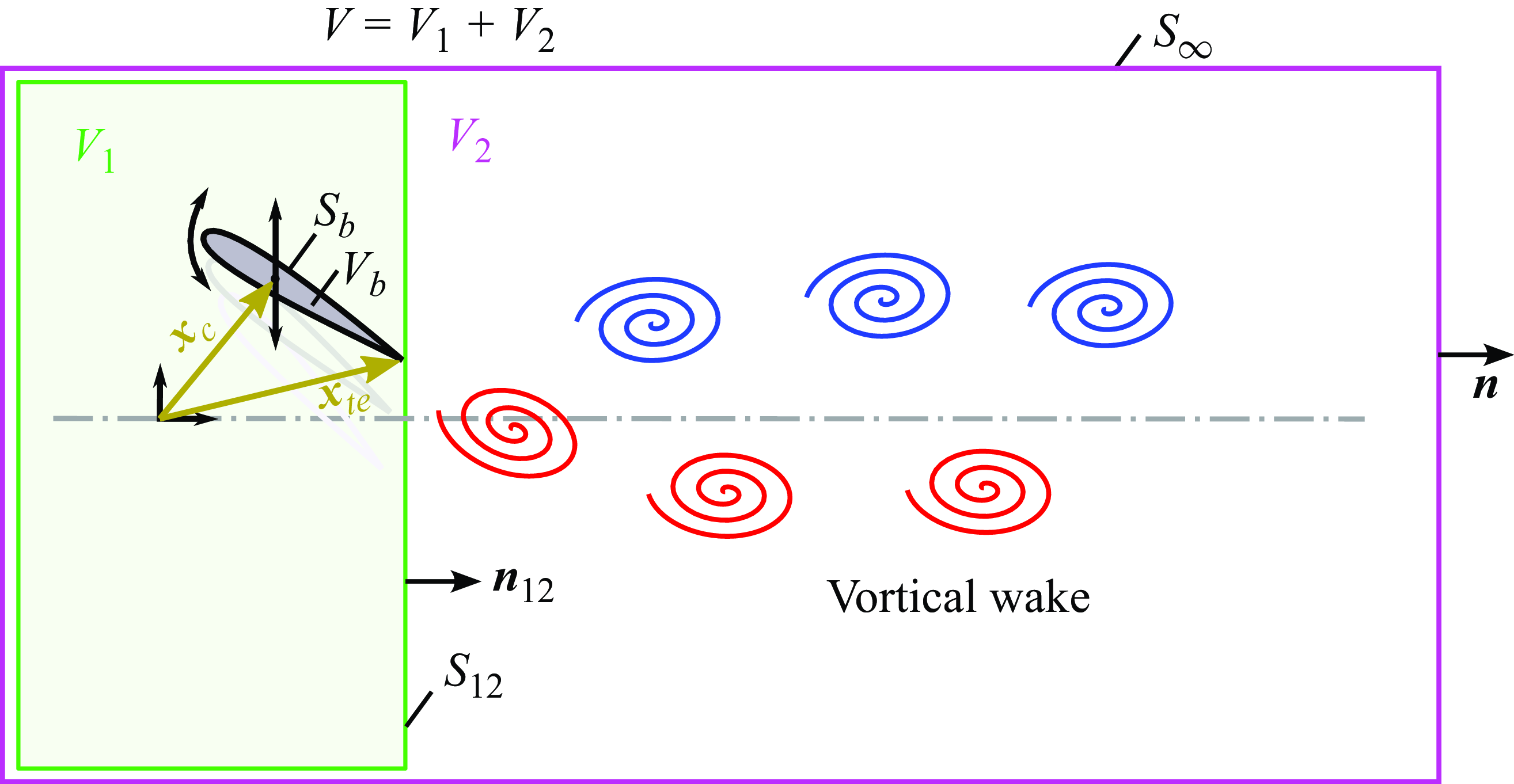
Figure 1. Schematic showing the two-dimensional control volumes ( $V,V_1,V_2$
), the bounding contours (
$V,V_1,V_2$
), the bounding contours ( $S_b,S_{12},S_\infty$
), the normal vectors (
$S_b,S_{12},S_\infty$
), the normal vectors ( $n, n_{12}$
), and the position vectors (
$n, n_{12}$
), and the position vectors ( $x_{c}, x_{te}$
) used in the present derivation. The cartoon vortices indicate that the wake is contained in
$x_{c}, x_{te}$
) used in the present derivation. The cartoon vortices indicate that the wake is contained in $V_2$
, although no specific wake structure is assumed in the derivation.
$V_2$
, although no specific wake structure is assumed in the derivation.
For the present analysis, the two-dimensional control volumes shown in figure 1 will be used. Here, $V$
is the fluid domain, externally bounded by a static contour
$V$
is the fluid domain, externally bounded by a static contour $S_\infty$
, far from the body, and internally bounded by the solid body surface,
$S_\infty$
, far from the body, and internally bounded by the solid body surface, $S_b$
. It will be assumed that the onset of fluid motion was a finite time ago, such that no vorticity will have yet approached nor crossed
$S_b$
. It will be assumed that the onset of fluid motion was a finite time ago, such that no vorticity will have yet approached nor crossed $S_\infty$
, such that the total circulation around
$S_\infty$
, such that the total circulation around $S_\infty$
is zero at all times. The undisturbed free-stream flow far from the body is
$S_\infty$
is zero at all times. The undisturbed free-stream flow far from the body is ${\boldsymbol{U}}_\infty$
.
${\boldsymbol{U}}_\infty$
.
To relate the force on the foil, $\boldsymbol{F}$
, to the incompressible flow field in
$\boldsymbol{F}$
, to the incompressible flow field in $V$
under these conditions (and the additional condition that non-conservative body forces are absent), one could apply conservation of momentum in a conventional manner to obtain
$V$
under these conditions (and the additional condition that non-conservative body forces are absent), one could apply conservation of momentum in a conventional manner to obtain
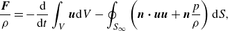 \begin{equation} \frac {{\boldsymbol{F}}}{\rho } = -\frac {\rm d}{{\rm d}t} \int _V {\boldsymbol{u}} {\rm d}V - \oint _{S_\infty } \left ( \boldsymbol{n} \boldsymbol{\cdot} {\boldsymbol{u}} {\boldsymbol{u}} + \boldsymbol{n} \frac {p}{\rho } \right ) {\rm d}S, \end{equation}
where $\boldsymbol{n}$
is the outward facing normal vector on
$\boldsymbol{n}$
is the outward facing normal vector on $S_\infty$
,
$S_\infty$
, ${\boldsymbol{u}} = {\boldsymbol{u}}({\boldsymbol{x}},t)$
represents the velocity field, and
${\boldsymbol{u}} = {\boldsymbol{u}}({\boldsymbol{x}},t)$
represents the velocity field, and $p = p({\boldsymbol{x}},t)$
the static pressure field, where
$p = p({\boldsymbol{x}},t)$
the static pressure field, where $\boldsymbol{x}$
is the vector position in the chosen coordinate system. In (3.1) and elsewhere, the arguments of the field parameters are omitted to allow compact expressions. No viscous-stress term appears in (3.1) due to the absence of vorticity (or vorticity gradients) on
$\boldsymbol{x}$
is the vector position in the chosen coordinate system. In (3.1) and elsewhere, the arguments of the field parameters are omitted to allow compact expressions. No viscous-stress term appears in (3.1) due to the absence of vorticity (or vorticity gradients) on $S_\infty$
.
$S_\infty$
.
Rather than express force in terms of velocity and pressure, it will be more fruitful to express it in terms of velocity and vorticity. Noca (Reference Noca1997) and Wu et al. (Reference Wu, Ma and Zhou2015) show how (3.1) can be manipulated to yield
 \begin{equation} \frac {{\boldsymbol{F}}}{\rho } = -\frac {\rm d}{{\rm d}t} \int _V {\boldsymbol{x}} \times \boldsymbol{\omega }\, {\rm d}V - \frac {\rm d}{{\rm d}t} \oint _{S_b} {\boldsymbol{x}} \times (\boldsymbol{n} \times {\boldsymbol{u}})\, {\rm d}S, \end{equation}
where $\boldsymbol{\omega } = \boldsymbol{\omega }({\boldsymbol{x}},t)$
is the vorticity vector (normal to the plane of the page), the unit normal
$\boldsymbol{\omega } = \boldsymbol{\omega }({\boldsymbol{x}},t)$
is the vorticity vector (normal to the plane of the page), the unit normal $\boldsymbol{n}$
is oriented into the fluid on
$\boldsymbol{n}$
is oriented into the fluid on $S_b$
, and the choice of origin for
$S_b$
, and the choice of origin for $\boldsymbol{x}$
has no effect on force due to the zero circulation around
$\boldsymbol{x}$
has no effect on force due to the zero circulation around $S_\infty$
. Equation (3.2) is an exact alternative expression of linear momentum conservation, placing no further restrictions than those inherent to (3.1). The first integral on the right-hand side of (3.2) is commonly referred to as vortical impulse, or simply impulse, and the body of work based on this and related equations is sometimes referred to as vortical impulse theory. I prefer the more general term ‘vortical flow theory’ to capture cases in which this equation is manipulated to remove the explicit appearance of vortical impulse (as will be done herein), but in which the primitive variables remain velocity and vorticity.
$S_\infty$
. Equation (3.2) is an exact alternative expression of linear momentum conservation, placing no further restrictions than those inherent to (3.1). The first integral on the right-hand side of (3.2) is commonly referred to as vortical impulse, or simply impulse, and the body of work based on this and related equations is sometimes referred to as vortical impulse theory. I prefer the more general term ‘vortical flow theory’ to capture cases in which this equation is manipulated to remove the explicit appearance of vortical impulse (as will be done herein), but in which the primitive variables remain velocity and vorticity.
Note how (3.2) is a generalisation of (2.2). If the body is of zero volume and the no-slip condition is applied on $S_b$
, then the integral over
$S_b$
, then the integral over $S_b$
can be shown to vanish (Wu Reference Wu1981; Limacher et al. Reference Limacher, Morton and Wood2018); if one then further assumes the pitch angle to be approximately zero and the wake to be aligned with the free-stream direction, (2.2) is recovered.
$S_b$
can be shown to vanish (Wu Reference Wu1981; Limacher et al. Reference Limacher, Morton and Wood2018); if one then further assumes the pitch angle to be approximately zero and the wake to be aligned with the free-stream direction, (2.2) is recovered.
We now divide the control volume, $V$
, into two: one encompassing the foil,
$V$
, into two: one encompassing the foil, $V_1$
, with a downstream surface just behind the trailing edge and moving with it; and
$V_1$
, with a downstream surface just behind the trailing edge and moving with it; and $V_2$
encompassing the wake. Now, rather than explicitly imposing the no-slip condition as just described, Limacher et al. (Reference Limacher, Morton and Wood2018) manipulated the body-surface integral in (3.2) by applying a Helmholtz decomposition to the velocity field, yielding a force expression which is valid for rigid two-dimensional bodies, with no further restriction on motion:
$V_2$
encompassing the wake. Now, rather than explicitly imposing the no-slip condition as just described, Limacher et al. (Reference Limacher, Morton and Wood2018) manipulated the body-surface integral in (3.2) by applying a Helmholtz decomposition to the velocity field, yielding a force expression which is valid for rigid two-dimensional bodies, with no further restriction on motion:
 \begin{equation} \frac {{\boldsymbol{F}}}{\rho } = -\frac {\rm d}{{\rm d}t} \left [ \int _V {\boldsymbol{x}} \times \boldsymbol{\omega }\, {\rm d}V + \int _{V_b} {\boldsymbol{x}} \times \boldsymbol{\omega }\, {\rm d}V - \oint _{S_b} \boldsymbol{n} \phi ^\prime {\rm d}S - {\boldsymbol{u}}_c v_b \right ], \end{equation}
where $V_b$
is the region occupied by the solid body,
$V_b$
is the region occupied by the solid body, $v_b$
is the volume of that space (zero for a thin foil), and
$v_b$
is the volume of that space (zero for a thin foil), and ${\boldsymbol{u}}_c$
is the velocity of the body centroid. Here,
${\boldsymbol{u}}_c$
is the velocity of the body centroid. Here, $\phi ^\prime$
is the acyclic (i.e. circulation-free) scalar potential associated with the irrotational component of the velocity field, defined such that
$\phi ^\prime$
is the acyclic (i.e. circulation-free) scalar potential associated with the irrotational component of the velocity field, defined such that $\nabla \phi ^\prime$
gives a velocity in the body-fixed frame of reference. That is,
$\nabla \phi ^\prime$
gives a velocity in the body-fixed frame of reference. That is, $\phi ^\prime$
is the solution to the Laplace equation on
$\phi ^\prime$
is the solution to the Laplace equation on $V$
, subject to the boundary conditions
$V$
, subject to the boundary conditions $\boldsymbol{n} \boldsymbol{\cdot} \nabla \phi ^\prime = 0$
on
$\boldsymbol{n} \boldsymbol{\cdot} \nabla \phi ^\prime = 0$
on $S_b$
and
$S_b$
and $\nabla \phi ^\prime = {\boldsymbol{U}}_\infty - {\boldsymbol{u}}_c$
on
$\nabla \phi ^\prime = {\boldsymbol{U}}_\infty - {\boldsymbol{u}}_c$
on $S_\infty$
. When the sum of these last two terms is differentiated with respect to time, it gives rise to the classical added-mass force,
$S_\infty$
. When the sum of these last two terms is differentiated with respect to time, it gives rise to the classical added-mass force, ${\boldsymbol{F}}_{\def\negativespace{}am}$
(Limacher et al. Reference Limacher, Morton and Wood2018; Limacher Reference Limacher2021):
${\boldsymbol{F}}_{\def\negativespace{}am}$
(Limacher et al. Reference Limacher, Morton and Wood2018; Limacher Reference Limacher2021):
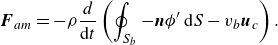 \begin{equation} {\boldsymbol{F}}_{\def\negativespace{}am} = -\rho \frac {d}{{\rm d}t} \left (\oint _{S_b} -\boldsymbol{n} \phi ^\prime\, {\rm d}S - v_b {\boldsymbol{u}}_c\right ). \end{equation}
The added-mass force, thusly defined, is calculable directly from the instantaneous motion and geometry of the body, with no dependence on the transient vorticity field. Unfortunately, the term ‘added-mass’ is defined in multiple ways in the literature, and confusion arises due to equivocation on its definition. The present definition is the same as that used by Sedov (Reference Sedov1965); Brennen (Reference Brennen1982), Floryan et al. (Reference Floryan, Van Buren, Rowley and Smits2017), Limacher et al. (Reference Limacher, Morton and Wood2018) and Limacher (Reference Limacher2021), but different from empirical definitions of added mass (e.g. Williamson & Govardhan Reference Williamson and Govardhan2004).
The integral in (3.3) over $V_b$
is referred to as the image-vorticity impulse. This is a familiar concept from potential-flow modelling, but it is valid for continuous distributions of vorticity as well (Saffman Reference Saffman1992). The effect of the solid body on the surrounding fluid is captured by treating the body as if occupied by fluid with a special vorticity distribution within it; to be valid, this vorticity distribution must exactly cancel any velocity induced by the wake that would violate the impermeable boundary condition. In general, there are infinitely many such candidate distributions, but we are assured by Saffman (Reference Saffman1992) that each of these has the same impulse, and therefore the same effect on force. The image-vorticity distribution may even be confined to lie on the body surface as a vortex sheet, degenerating to a single line of vorticity in the case of a thin uncambered foil.
$V_b$
is referred to as the image-vorticity impulse. This is a familiar concept from potential-flow modelling, but it is valid for continuous distributions of vorticity as well (Saffman Reference Saffman1992). The effect of the solid body on the surrounding fluid is captured by treating the body as if occupied by fluid with a special vorticity distribution within it; to be valid, this vorticity distribution must exactly cancel any velocity induced by the wake that would violate the impermeable boundary condition. In general, there are infinitely many such candidate distributions, but we are assured by Saffman (Reference Saffman1992) that each of these has the same impulse, and therefore the same effect on force. The image-vorticity distribution may even be confined to lie on the body surface as a vortex sheet, degenerating to a single line of vorticity in the case of a thin uncambered foil.
Let us now split the contributions of the impulse and image-vorticity impulse into those arising from vorticity in the mutually exclusive subdomains $V_1 \subset V$
and
$V_1 \subset V$
and $V_2 \subset V$
, where
$V_2 \subset V$
, where $V = V_1 \cup V_2$
. The domain
$V = V_1 \cup V_2$
. The domain $V_1$
deforms such that the boundary
$V_1$
deforms such that the boundary $S_{12}$
separating
$S_{12}$
separating $V_1$
and
$V_1$
and $V_2$
always lies directly behind the trailing edge. This definition neatly divides the vorticity field into that which exists in attached boundary layers on the body (in
$V_2$
always lies directly behind the trailing edge. This definition neatly divides the vorticity field into that which exists in attached boundary layers on the body (in $V_1$
) and that which lies in the wake (
$V_1$
) and that which lies in the wake ( $V_2$
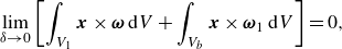
). Under the assumption that the attached boundary-layer thickness,
$V_2$
). Under the assumption that the attached boundary-layer thickness, $\delta$
, tends to zero, we note that
$\delta$
, tends to zero, we note that
 \begin{equation} \lim _{\delta \rightarrow 0} \left [ \int _{V_1} {\boldsymbol{x}} \times \boldsymbol{\omega }\, {\rm d}V + \int _{V_b} {\boldsymbol{x}}\times \boldsymbol{\omega }_1\, {\rm d}V \right ] = 0, \end{equation}
where $\boldsymbol{\omega }_1$
is the image vorticity associated with the physical vorticity in
$\boldsymbol{\omega }_1$
is the image vorticity associated with the physical vorticity in $V_1$
. For those familiar with the image-vortex concept for the potential flow around a circle, recall that as a point vortex approaches the boundary of the circle, its image approaches the same point from inside the circle (e.g. Milne-Thomson Reference Milne-Thomson1960), such that their associated impulses tend to cancel. Equation (3.5) is a generalisation of this idea to two-dimensional shapes of arbitrary geometry (see § 7.1 of Limacher (Reference Limacher2019)).
$V_1$
. For those familiar with the image-vortex concept for the potential flow around a circle, recall that as a point vortex approaches the boundary of the circle, its image approaches the same point from inside the circle (e.g. Milne-Thomson Reference Milne-Thomson1960), such that their associated impulses tend to cancel. Equation (3.5) is a generalisation of this idea to two-dimensional shapes of arbitrary geometry (see § 7.1 of Limacher (Reference Limacher2019)).
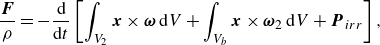
As a result of the cancellation in (3.5), the force can be expressed as
 \begin{equation} \frac {{\boldsymbol{F}}}{\rho } = -\frac {\rm d}{{\rm d}t} \left [ \int _{V_2} {\boldsymbol{x}} \times \boldsymbol{\omega }\, {\rm d}V + \int _{V_b} {\boldsymbol{x}} \times \boldsymbol{\omega }_2\, {\rm d}V + \boldsymbol{P}_{\def\negativespace{}irr} \right ], \end{equation}
where $\boldsymbol{\omega }_2$
is the image vorticity associated with the physical vorticity in
$\boldsymbol{\omega }_2$
is the image vorticity associated with the physical vorticity in $V_2$
, and
$V_2$
, and $\boldsymbol{P}_{\def\negativespace{}irr}$
is the sum of the terms in brackets in (3.4). The
$\boldsymbol{P}_{\def\negativespace{}irr}$
is the sum of the terms in brackets in (3.4). The $V_2$
integral can be manipulated through the Reynolds transport theorem:
$V_2$
integral can be manipulated through the Reynolds transport theorem:
 \begin{equation} \frac {\rm d}{{\rm d}t} \int _{V_2} {\boldsymbol{x}} \times \boldsymbol{\omega } {\rm d}V = \frac {\rm d}{{\rm d}t} \int _{V_m} {\boldsymbol{x}} \times \boldsymbol{\omega }\, {\rm d}V + \oint _{S_{12}} \boldsymbol{n} \boldsymbol{\cdot} ({\boldsymbol{u}}-{\boldsymbol{u}}_s) ({\boldsymbol{x}}\times \boldsymbol{\omega })\, {\rm d}S, \end{equation}
where $\boldsymbol{n}$
is the unit normal on
$\boldsymbol{n}$
is the unit normal on $S_{12}$
, pointing into
$S_{12}$
, pointing into $V_2$
;
$V_2$
; ${\boldsymbol{u}}_s$
is the local velocity of the deforming contour
${\boldsymbol{u}}_s$
is the local velocity of the deforming contour $S_{12}$
; and
$S_{12}$
; and $V_m = V_m(t)$
is a material volume coincident with
$V_m = V_m(t)$
is a material volume coincident with $V_2 = V_2(t)$
at a given moment,
$V_2 = V_2(t)$
at a given moment, $t$
. Under this condition, we may treat the position variable
$t$
. Under this condition, we may treat the position variable $\boldsymbol{x}$
as a Lagrangian position variable, such that
$\boldsymbol{x}$
as a Lagrangian position variable, such that ${\boldsymbol{u}} = {\rm d}{\boldsymbol{x}}/{\rm d}t$
, and we can move the time-derivative operator inside the integral to yield the following expression, found also in the appendix of Kang et al. (Reference Kang, Liu, Su and Wu2017):
${\boldsymbol{u}} = {\rm d}{\boldsymbol{x}}/{\rm d}t$
, and we can move the time-derivative operator inside the integral to yield the following expression, found also in the appendix of Kang et al. (Reference Kang, Liu, Su and Wu2017):
 \begin{align} \frac {\rm d}{{\rm d}t}\int _{V_m} {\boldsymbol{x}} \times \boldsymbol{\omega } {\rm d}V &= \int _{V_m} {\boldsymbol{u}}\times \boldsymbol{\omega }\, {\rm d}V + \int _{V_m} {\boldsymbol{x}} \times \frac {\rm {D}\boldsymbol{\omega }}{{\rm {D}}t} {\rm d}V = \int _{V_2} {\boldsymbol{u}}\times \boldsymbol{\omega }\, {\rm d}V + \int _{V_2} {\boldsymbol{x}} \times \frac {\rm {D}\boldsymbol{\omega }}{{\rm{D}}t}\, {\rm d}V. \end{align}
where ${\rm {D}}/{\rm {D}}t$
denotes a material-derivative. In the limit of small viscosity, we can neglect this last term that denotes the effect of viscous diffusion in the wake.
${\rm {D}}/{\rm {D}}t$
denotes a material-derivative. In the limit of small viscosity, we can neglect this last term that denotes the effect of viscous diffusion in the wake.
The impulse-flux term – i.e. the last term in (3.7) – can be written as
 \begin{equation} \oint _{S_{12}} \boldsymbol{n} \cdot ({\boldsymbol{u}}- {\boldsymbol{u}}_s) ({\boldsymbol{x}}\times \boldsymbol{\omega })\, {\rm d}S \approx {\boldsymbol{x}}_{te} \times \oint _{S_{12}} \boldsymbol{n} \boldsymbol{\cdot} ({\boldsymbol{u}}-{\boldsymbol{u}}_s) \boldsymbol{\omega }\, {\rm d}S = {\boldsymbol{x}}_{te} \times \frac {{\rm d}\boldsymbol{\Gamma }_2}{{\rm d}t}, \end{equation}
where $\boldsymbol{\Gamma }_2$
is the total vector circulation of the wake in
$\boldsymbol{\Gamma }_2$
is the total vector circulation of the wake in $V_2$
, pointing out of the page when the circulation is anticlockwise, and
$V_2$
, pointing out of the page when the circulation is anticlockwise, and ${\boldsymbol{x}}_{te}$
is the location of the trailing edge. The first and second expressions in (3.9) are approximately equated because, under the attached-flow and thin-boundary-layer assumptions,
${\boldsymbol{x}}_{te}$
is the location of the trailing edge. The first and second expressions in (3.9) are approximately equated because, under the attached-flow and thin-boundary-layer assumptions, ${\boldsymbol{x}}_{te}$
is the only location at which vorticity crosses
${\boldsymbol{x}}_{te}$
is the only location at which vorticity crosses $S_{12}$
(or to be precise, the boundary layers leaving the trailing edge are spread over a thin region around
$S_{12}$
(or to be precise, the boundary layers leaving the trailing edge are spread over a thin region around ${\boldsymbol{x}}_{te}$
). Furthermore, with no solid body present in
${\boldsymbol{x}}_{te}$
). Furthermore, with no solid body present in $V_2$
and with diffusive flux assumed negligible on
$V_2$
and with diffusive flux assumed negligible on $S_{12}$
, the vorticity deposited into the wake by the trailing edge is the only means by which
$S_{12}$
, the vorticity deposited into the wake by the trailing edge is the only means by which $\boldsymbol{\Gamma }_2$
varies, such that the vorticity-flux integral in the second expression is equal to
$\boldsymbol{\Gamma }_2$
varies, such that the vorticity-flux integral in the second expression is equal to ${\rm d}\boldsymbol{\Gamma }_2/{\rm d}t$
in the third expression.
${\rm d}\boldsymbol{\Gamma }_2/{\rm d}t$
in the third expression.
Substituting (3.7)–(3.9) into (3.6), we obtain
 \begin{equation} \frac {{\boldsymbol{F}}}{\rho } = - \int _{V_2} {\boldsymbol{u}}\times \boldsymbol{\omega }\, {\rm d}V - \frac {\rm d}{{\rm d}t} \int _{V_b} {\boldsymbol{x}}\times \boldsymbol{\omega }_2\, {\rm d}V - {\boldsymbol{x}}_{te} \times \frac {{\rm d}\boldsymbol{\Gamma }_2}{{\rm d}t} - \frac { {\rm d}\boldsymbol{P}_{\def\negativespace{}irr}}{{\rm d}t}. \end{equation}
It may still appear that we need complete knowledge of the transient vortical wake to calculate force, but, in fact, we need only know certain wake-averaged quantities. Let us define the vorticity-weighted wake convection velocity, $\overline {{\boldsymbol{u}}}_w$
, as
$\overline {{\boldsymbol{u}}}_w$
, as
 \begin{equation} \overline {{\boldsymbol{u}}}_w := \frac {1}{\Gamma _2} \int _{V_2}{\boldsymbol{u}}\omega\, {\rm d}V, \end{equation}
where $\Gamma _2$
and
$\Gamma _2$
and $\omega$
are the circulation and vorticity magnitudes (positive anticlockwise), respectively, such that
$\omega$
are the circulation and vorticity magnitudes (positive anticlockwise), respectively, such that
 \begin{equation} \overline {{\boldsymbol{u}}}_w \times \boldsymbol{\Gamma }_2 = \int _{V_2} {\boldsymbol{u}}\times \boldsymbol{\omega }\, {\rm d}V. \end{equation}
Of course, (3.11) is not defined at moments when $\Gamma _2 = 0$
, but this is not expected to impede attempts at modelling, because
$\Gamma _2 = 0$
, but this is not expected to impede attempts at modelling, because $\overline {{\boldsymbol{u}}}_w$
is expected to remain bounded and well-behaved in the sense that
$\overline {{\boldsymbol{u}}}_w$
is expected to remain bounded and well-behaved in the sense that
 \begin{equation} \lim _{t\rightarrow t_0^-} \overline {{\boldsymbol{u}}}_w = \lim _{t\rightarrow t_0^ + } \overline {{\boldsymbol{u}}}_w, \end{equation}
where $t_0$
is the moment at which the circulation is zero, and
$t_0$
is the moment at which the circulation is zero, and $t \rightarrow t_0^-$
and
$t \rightarrow t_0^-$
and $t \rightarrow 0^+$
indicate time approaching
$t \rightarrow 0^+$
indicate time approaching $t_0$
from the left and right, respectively. This must be true because, for a realistic flow with non-zero viscosity, we expect velocity and vorticity everywhere in
$t_0$
from the left and right, respectively. This must be true because, for a realistic flow with non-zero viscosity, we expect velocity and vorticity everywhere in $V_2$
to be continuous in both space and time; although the boundary layers have been assumed thin, they are not defined as singular vortex sheets. Accordingly, gradients of velocity or vorticity may be arbitrarily large in
$V_2$
to be continuous in both space and time; although the boundary layers have been assumed thin, they are not defined as singular vortex sheets. Accordingly, gradients of velocity or vorticity may be arbitrarily large in $V$
but still finite, and if the foil motion is smooth in time, the resulting flow field should be likewise smooth. The integral on the right-hand side of (3.12) will thus be a continuous function of time, as will
$V$
but still finite, and if the foil motion is smooth in time, the resulting flow field should be likewise smooth. The integral on the right-hand side of (3.12) will thus be a continuous function of time, as will $\boldsymbol{\Gamma }_2$
on the left-hand side; from these assertions it follows that
$\boldsymbol{\Gamma }_2$
on the left-hand side; from these assertions it follows that $\overline {{\boldsymbol{u}}}_w$
cannot be discontinuous at any moment in time, regardless of the instantaneous value of
$\overline {{\boldsymbol{u}}}_w$
cannot be discontinuous at any moment in time, regardless of the instantaneous value of $\Gamma _2$
.
$\Gamma _2$
.
We may now similarly define the centroid of the image-vorticity distribution, relative to the body centroid ( ${\boldsymbol{x}}_c$
), as
${\boldsymbol{x}}_c$
), as
 \begin{equation} \overline {{\boldsymbol{x}}}_i^\prime := -\frac {1}{\Gamma _2} \int _{V_b} {\boldsymbol{x}} \omega _2\, {\rm d}V - {\boldsymbol{x}}_c, \end{equation}
such that
 \begin{equation} ({\boldsymbol{x}}_c + \overline {{\boldsymbol{x}}}_i^\prime ) \times \boldsymbol{\Gamma }_2 = -\int _{V_b} {\boldsymbol{x}}\times \boldsymbol{\omega }_2\, {\rm d}V, \end{equation}
where the negative sign on the right-hand side is necessary because the image-vorticity distribution is of opposite sign to the physical vorticity distribution in $V_2$
. The same caveats apply when
$V_2$
. The same caveats apply when $\Gamma _2 = 0$
as were just noted for the definition of
$\Gamma _2 = 0$
as were just noted for the definition of $\overline {{\boldsymbol{u}}}_w$
.
$\overline {{\boldsymbol{u}}}_w$
.
One last relation is required: the total vorticity theorem of Wu (Reference Wu1981) is expressed as
 \begin{equation} \boldsymbol{\Gamma } + \boldsymbol{\Gamma }_2 = 0, \end{equation}
where $\boldsymbol{\Gamma }$
is the circulation around
$\boldsymbol{\Gamma }$
is the circulation around $S_{12}$
. In the case of a foil of finite volume, this must include not only the circulation associated with vorticity in the boundary layers, but also the circulation associated with the rotation of the foil itself. That is, for a rigid foil,
$S_{12}$
. In the case of a foil of finite volume, this must include not only the circulation associated with vorticity in the boundary layers, but also the circulation associated with the rotation of the foil itself. That is, for a rigid foil,
 \begin{equation} \boldsymbol{\Gamma } = \int _{V_1} \boldsymbol{\omega } {\rm d}V + 2 \boldsymbol{\Omega } v_b, \end{equation}
where $\boldsymbol{\Omega }$
is the rotation rate of the rigid body.
$\boldsymbol{\Omega }$
is the rotation rate of the rigid body.
Substituting (3.4), (3.12), (3.15) and (3.16) into (3.10) and rearranging, we obtain the primary result of this paper:
 \begin{equation} \frac {{\boldsymbol{F}}}{\rho } = (\overline {{\boldsymbol{u}}}_w - {\boldsymbol{u}}_c)\times \boldsymbol{\Gamma } + ({\boldsymbol{x}}_{te}-{\boldsymbol{x}}_c)\times \frac {{\rm d}\boldsymbol{\Gamma }}{{\rm d}t} - \frac {\rm d}{{\rm d}t}\big (\overline {{\boldsymbol{x}}}_i^\prime \times \boldsymbol{\Gamma }) + \frac {{\boldsymbol{F}}_{\def\negativespace{}am}}{\rho }. \end{equation}
When constructing a predictive model from (3.18), the image-vorticity term is likely the least intuitive because it is not an observable quantity; it is, however, directly calculable from the observable vorticity distribution in the wake. The reader is referred to section IV of Limacher et al. (Reference Limacher, Morton and Wood2018) for a generalisable approach to doing so.
An important ‘sanity check’ is to observe that (3.18) recovers the Kutta–Joukowsky lift theorem under the condition of steady motion. When circulation has reached steady state and the starting vortex system is convecting at a velocity of ${\boldsymbol{U}}_\infty$
far from the body, only the first term remains to yield
${\boldsymbol{U}}_\infty$
far from the body, only the first term remains to yield ${\boldsymbol{F}} = \rho {\boldsymbol{U}} \times \boldsymbol{\Gamma }$
, where
${\boldsymbol{F}} = \rho {\boldsymbol{U}} \times \boldsymbol{\Gamma }$
, where ${\boldsymbol{U}} := {\boldsymbol{U}}_\infty - {\boldsymbol{u}}_c$
.
${\boldsymbol{U}} := {\boldsymbol{U}}_\infty - {\boldsymbol{u}}_c$
.
4. Mean forces on an oscillating foil
To consider the generation of mean forces on continuously oscillating foils, let us adopt the following notation to denote cycle-averaged parameters:
 \begin{equation} \langle \cdot \rangle := \frac {1}{T} \int _t^{t + T} \cdot \text{ }{\rm d}t, \end{equation}
where $T$
is the period (in units of time) and the
$T$
is the period (in units of time) and the $\cdot$
can be replaced by any parameter of interest. Here,
$\cdot$
can be replaced by any parameter of interest. Here, $T$
may be set equal to the period of foil oscillation, or if needed, it may be set equal to a multi-cycle period to capture the effect of cycle-to-cycle variations in the flow.
$T$
may be set equal to the period of foil oscillation, or if needed, it may be set equal to a multi-cycle period to capture the effect of cycle-to-cycle variations in the flow.
Many of the force components in (3.18) will not contribute to cycle-averaged forces because they are expressible as derivatives of periodic quantities. Noting that
 \begin{equation} {\boldsymbol{u}}_c \times \boldsymbol{\Gamma } + {\boldsymbol{x}}_c \times \frac {{\rm d}\boldsymbol{\Gamma }}{{\rm d}t} = \frac {\rm d}{{\rm d}t} ({\boldsymbol{x}}_{c} \times \boldsymbol{\Gamma }), \end{equation}
we can rearrange (3.18) and group all these derivative terms together:
 \begin{equation} \frac { {\boldsymbol{F}} }{\rho } = \overline {{\boldsymbol{u}}}_w \times \boldsymbol{\Gamma } + {\boldsymbol{x}}_{te}\times \frac {{\rm d}\boldsymbol{\Gamma }}{{\rm d}t} - \frac {\rm d}{{\rm d}t} \left ({\boldsymbol{x}}_c \times \boldsymbol{\Gamma } + \overline {{\boldsymbol{x}}}_i^\prime \times \boldsymbol{\Gamma } + \boldsymbol{P}_{\def\negativespace{}irr} \right ). \end{equation}
The parameter ${\boldsymbol{x}}_c$
is periodic by the definition of oscillatory motion, and
${\boldsymbol{x}}_c$
is periodic by the definition of oscillatory motion, and $\boldsymbol{\Gamma }$
is expected to become periodic once the wake is well established;
$\boldsymbol{\Gamma }$
is expected to become periodic once the wake is well established; $\boldsymbol{P}_{\def\negativespace{}irr}$
is also periodic, as it depends only on instantaneous motion and geometry. Only
$\boldsymbol{P}_{\def\negativespace{}irr}$
is also periodic, as it depends only on instantaneous motion and geometry. Only $\overline {{\boldsymbol{x}}}_i^\prime$
requires further thought to be recognised as periodic.
$\overline {{\boldsymbol{x}}}_i^\prime$
requires further thought to be recognised as periodic.
Imagine a continuously developing wake that convects away from the foil, growing in downstream extent with every cycle. After one more cycle, the wake appears to be the same wake plus an additional vorticity distribution aggregated to the end of the wake. If the wake is sufficiently long, the velocity induced at the foil by this newly added wake section is negligible, and thus it cannot significantly affect the image-vorticity distribution nor the total bound circulation. Thus, after the wake is sufficiently long (but not infinitely long to ensure no vorticity reaches $S_\infty$
), the parameter
$S_\infty$
), the parameter $\overline {{\boldsymbol{x}}}_i^\prime$
is negligibly affected by the continued extension of the far wake from cycle to cycle, and thus it becomes periodic.
$\overline {{\boldsymbol{x}}}_i^\prime$
is negligibly affected by the continued extension of the far wake from cycle to cycle, and thus it becomes periodic.
When (4.3) is cycle-averaged, the far-right grouping of terms vanishes, and we are left with
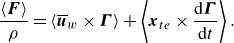 \begin{equation} \frac {\langle {\boldsymbol{F}} \rangle }{\rho } = \langle \overline {{\boldsymbol{u}}}_w \times \boldsymbol{\Gamma } \rangle + \left\langle {\boldsymbol{x}}_{te}\times \frac {{\rm d}\boldsymbol{\Gamma }}{{\rm d}t} \right \rangle . \end{equation}
Consider the case where the wake convects parallel to the free-stream direction and the trailing edge oscillates only in the transverse direction; the two terms on the right-hand side of (4.4) are then pure lift and drag (or thrust), respectively. If we add the further condition that $\overline {{\boldsymbol{u}}}_w = \overline {{\boldsymbol{U}}}_w$
, where
$\overline {{\boldsymbol{u}}}_w = \overline {{\boldsymbol{U}}}_w$
, where $\overline {{\boldsymbol{U}}}_w$
is constant, we obtain
$\overline {{\boldsymbol{U}}}_w$
is constant, we obtain
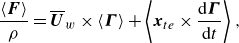 \begin{equation} \frac {\langle {\boldsymbol{F}} \rangle }{\rho } = \overline {{\boldsymbol{U}}}_w \times \langle \boldsymbol{\Gamma } \rangle + \left\langle {\boldsymbol{x}}_{te}\times \frac {{\rm d}\boldsymbol{\Gamma }}{{\rm d}t} \right \rangle , \end{equation}
and we see that the lift is given by a Kutta–Joukowsky-like term, dependent on the mean circulation.
As for the streamwise force, the importance of the trailing-edge position becomes clear; all else being equal, an increase in the amplitude of a transverse trailing-edge oscillation will increase the mean streamwise force generated. This is in agreement with the theoretical treatment of Chopra (Reference Chopra1976), who derived a positive correlation between trailing-edge amplitude and mean thrust coefficient.
Equation (4.5) also elicits speculative hypotheses for flexible-foil propulsors. Consider a foil driven transversely to the free stream from some mounting point ahead of the trailing edge; increasing flexibility can amplify the motion of the trailing edge relative to the driving amplitude, potentially allowing for greater thrust generation for a given driving motion. One might speculate that this allows flexible foils to achieve greater propulsive efficiency than rigid ones, as has been observed (e.g. Dewey et al. Reference Dewey, Boschitsch, Moored, Stone and Smits2013). The actual change in mean forces, and associated power input, depends on how the circulation history is affected by flexibility (i.e. how its phase relative to the trailing-edge motion is altered). Further investigation along these lines will require a rederivation of (3.3) and (3.18) that is valid for flexible foils.
Equation (4.4) can be written even more compactly as
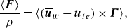 \begin{equation} \frac {\langle {\boldsymbol{F}} \rangle }{\rho } = \langle (\overline {{\boldsymbol{u}}}_w - {\boldsymbol{u}}_{te}) \times \boldsymbol{\Gamma } \rangle , \end{equation}
which is achieved by integration by parts, with ${\boldsymbol{u}}_{te}$
denoting the trailing-edge velocity. Inspection of this equation highlights the trailing-edge velocity as the velocity scale that governs thrust production on transversely oscillating propulsors, in agreement with empirical observations (Smits Reference Smits2019).
${\boldsymbol{u}}_{te}$
denoting the trailing-edge velocity. Inspection of this equation highlights the trailing-edge velocity as the velocity scale that governs thrust production on transversely oscillating propulsors, in agreement with empirical observations (Smits Reference Smits2019).
5. Conclusion
A new mathematical framework has been derived from vortical flow theory to serve as a basis to derive closed-form expressions for fluid-dynamic force on thick, rigid foils undergoing any type of motion in an incompressible fluid; the restriction of small-amplitude motion from classical unsteady aerofoil theory has been removed, but the limitation to attached flow has been retained. Viscosity is assumed to approach but not equal zero; likewise, boundary-layer thickness approaches but does not equal zero.
Starting from the derived ‘recipe’ in (3.18), one can concoct a closed-form aerodynamic model based on predictions for the following time-varying integral parameters: vorticity-weighted mean convection speed of the wake, $\overline {{\boldsymbol{u}}}_w$
; the bound circulation of the foil (including circulation associated with rotation of thick foils),
$\overline {{\boldsymbol{u}}}_w$
; the bound circulation of the foil (including circulation associated with rotation of thick foils), $\boldsymbol{\Gamma }$
; and the centroid location of the wake’s image-vorticity distribution,
$\boldsymbol{\Gamma }$
; and the centroid location of the wake’s image-vorticity distribution, $\overline {{\boldsymbol{x}}}_i^\prime$
. The geometry and motion of the foil must also be known. The circulation is left as a free parameter to be determined by any model one may choose, allowing one (in principle) to supersede the known limitations of the Kutta condition used to predict a unique circulation in potential-flow models.
$\overline {{\boldsymbol{x}}}_i^\prime$
. The geometry and motion of the foil must also be known. The circulation is left as a free parameter to be determined by any model one may choose, allowing one (in principle) to supersede the known limitations of the Kutta condition used to predict a unique circulation in potential-flow models.
An expression for the mean forces on oscillating foils was also derived (4.6), and it was shown that mean forces depend closely on trailing-edge velocities, in agreement with previous experimental observations. An alternative form of the same – equation (4.4) – highlights the importance of achieving large transverse trailing-edge displacements to generate large mean streamwise forces. The importance of the trailing edge in the derived equations is due to it being the only location from which vorticity is deposited into the wake, under the assumption of attached flow and thin boundary layers.
Funding
The author would like to thank the Natural Sciences and Engineering Research Council of Canada (NSERC) for funding this research.
Declaration of interests
The author reports no conflict of interest.


 Open access