





1. Introduction
A systematic resolution of the nonlinear dynamical transitions in the near and far wake of flapping bodies is still elusive. In the aperiodic and chaotic regimes, the aerodynamic loads acting on a flapping body can become unpredictable from one flapping cycle to another, posing significant challenges in designing suitable control algorithms for man-made flapping devices. Therefore, kinematic parameters that lead to aperiodic/chaotic flow dynamics are not desirable from the viewpoint of an efficient design of bio-inspired flapping devices like micro aerial vehicles. Identifying the transition onsets to determine a stable operating regime for such devices is important. Earlier studies in the literature are focused primarily on von Kármán to reverse von Kármán wake (drag-to-thrust) transition (Triantafyllou, Triantafyllou & Gopalkrishnan Reference Triantafyllou, Triantafyllou and Gopalkrishnan1991; Streitlien & Triantafyllou Reference Streitlien and Triantafyllou1998) and symmetric to deflected wake transition phenomena (Jones, Dohring & Platzer Reference Jones, Dohring and Platzer1998; Godoy-Diana et al. Reference Godoy-Diana, Marais, Aider and Wesfreid2009; Zheng & Wei Reference Zheng and Wei2012); note that both transitions happen in the periodic regime. However, a few recent studies have also highlighted interesting changes from periodicity to aperiodicity in the wake for different canonical flapping kinematics, e.g. pure plunging (Lewin & Haj-Hariri Reference Lewin and Haj-Hariri2003; Badrinath, Bose & Sarkar Reference Badrinath, Bose and Sarkar2017; Majumdar, Bose & Sarkar Reference Majumdar, Bose and Sarkar2020a), pure pitching (Zaman, Young & Lai Reference Zaman, Young and Lai2017) and combined pitching–plunging (Lentink et al. Reference Lentink, Van Heijst, Muijres and Van Leeuwen2010; Bose & Sarkar Reference Bose and Sarkar2018; Bose, Gupta & Sarkar Reference Bose, Gupta and Sarkar2021). Different local bifurcation routes to chaos, involving quasi-periodic and intermittent dynamical states, were reported in these studies.
Lentink et al. (Reference Lentink, Van Heijst, Muijres and Van Leeuwen2010), through two-dimensional (2-D) soap film experiments, presented chaotic wake patterns using phase-averaged vorticity contours. Bose & Sarkar (Reference Bose and Sarkar2018) and Bose et al. (Reference Bose, Gupta and Sarkar2021), through Navier–Stokes simulations, reported a quasi-periodic route, accompanied by sporadic intermittent windows of aperiodicity, towards a regime of robust chaos. The authors established that the time delay in the formation of the primary leading-edge vortex (LEV) was instrumental in ushering chaos in the wake. At high plunge velocities, the LEV sheds aperiodically, and subsequently, its irregular interactions with the trailing-edge vortex (TEV) gives way to chaos in the wake. The mechanism is sustained in the far wake through a variety of fundamental vortex interactions (such as vortex merging, collision, shredding, exchange of partners). Majumdar et al. (Reference Majumdar, Bose and Sarkar2020a) have also shown that the aperiodic transition is extremely sensitive to LEV behaviour, and any discrepancy in their formation, growth or transport may lead to a completely different dynamical state. Note that even though the effects of flapping amplitude and frequency were considered carefully in these earlier studies, some of the other important kinematic parameters, such as pitch amplitude, pitching axis location, phase offset and kinematic pattern, have received almost no attention in the existing literature. In the case of combined kinematics, it is likely that LEV separation, and in turn, the near-field interactions of vortices, will be altered significantly by varying these parameters. Furthermore, the ensuing change in the effective angle of attack (AoA) for combined pitch and plunge can also be crucial in dictating the flow field. Note that earlier studies that considered the variation of some of these parameters (Anderson et al. Reference Anderson, Streitlien, Barrett and Triantafyllou1998; Read, Hover & Triantafyllou Reference Read, Hover and Triantafyllou2003; Lee & Su Reference Lee and Su2015; Buren, Floryan & Smits Reference Buren, Floryan and Smits2019) focused primarily on their effect on aerodynamic force magnitudes and pressure distributions, and not on dynamical behaviour. No attempts have yet been made in the existing literature to consider the effects of all these relevant parametric combinations together and study the dynamical transitions to predict generalised bifurcation boundaries.
This leads to two interesting directions: first, can one identify suitable non-dimensional parameters that can capture the effects of different kinematic parameters together, and second, can one model generalised transition/bifurcation boundaries to demarcate the dynamical regimes to an acceptable level of accuracy, statistically? Traditionally, flow field transitions have been defined in terms of a diverse set of non-dimensional parameters. Godoy-Diana et al. (Reference Godoy-Diana, Marais, Aider and Wesfreid2009) demonstrated the wake transition for a pure pitching kinematics using an ‘ $A_D$ versus $St_D$’ plot, where $A_D$ is the thickness-based dimensionless amplitude, and $St_D$ is the thickness-based Strouhal number. Here, $A_D = A/D$, where $A$ and $D$ represent the peak-to-peak amplitude of the trailing edge and the maximum thickness of the foil, respectively; $St_D = f_eD/U_{\infty }$, where $f_e$ and $U_{\infty }$ denote the flapping frequency and free stream velocity, respectively. Deng et al. (Reference Deng, Sun, Teng, Pan and Shao2016) have used the same parameters and have presented periodic to chaotic transitions for increasing $St_D$ at a fixed $A_D$. Cleaver, Wang & Gursul (Reference Cleaver, Wang and Gursul2012) presented flow field bifurcations in terms of the chord-based Strouhal number $St_c$, where $St_c = f_e c/U_{\infty }$, with $c$ being the chord length. Triantafyllou et al. (Reference Triantafyllou, Triantafyllou and Gopalkrishnan1991) defined an amplitude-based Strouhal number as $St_A = f_e A/U_{\infty }$, to characterise the drag-to-thrust transition. It was proposed as the single key parameter that is a function of both flapping amplitude and frequency simultaneously. Lewin & Haj-Hariri (Reference Lewin and Haj-Hariri2003), Lentink et al. (Reference Lentink, Van Heijst, Muijres and Van Leeuwen2010) and Ashraf, Young & Lai (Reference Ashraf, Young and Lai2012), as well as the recent studies from our group (Bose & Sarkar Reference Bose and Sarkar2018; Majumdar et al. Reference Majumdar, Bose and Sarkar2020a), have considered the maximum non-dimensional plunge velocity ( $\kappa h$) as the main control parameter for wake transitions. Here, $\kappa h$ is proportional to $St_A$, where $\kappa = 2{\rm \pi} f_e c / U_{\infty }$ is called the reduced frequency and $h= h_0/c$ is the non-dimensional plunge amplitude.
Note that these existing non-dimensional parameters are not comprehensive enough to encompass the combined effects of different kinematic conditions. Previous studies that consider simple and unmixed kinematics, such as pure pitching or pure plunging, rely on a fixed set of dimensionless parameters that are effective enough to identify the changes in the flow field. However, they fall short in reflecting the combined effects of multiple parameters in a wholesome manner when more complex kinematics are used. These kinematic parameters include phase offsets between simple canonical kinematics and location of the pitching axis. Also, the parametric maps available in the literature for distinguishing qualitatively different wake regimes are strongly kinematic-specific and are mostly applicable to the periodic regime (low  $\kappa h$ or $St_A$). To address this issue, Lagopoulos, Weymouth & Ganapathisubramani (Reference Lagopoulos, Weymouth and Ganapathisubramani2019) have defined a path-length-based Strouhal number $St_\tau = f_e\tau /U_{\infty }$, where $\tau$ is the average trajectory length covered by the chord of the foil in one flapping period. It was reported that, irrespective of the flapping kinematics, drag-to-thrust transition takes place as $St_\tau$ crosses unity. However, the applicability of $St_\tau$ was confined to the periodic flow regime only ( $0.15 < St_D < 0.35$). No attempts have yet been made in the literature to demarcate the regimes of aperiodic transitions using a robust measure considering the combined effects of all the relevant kinematic parameters of importance. The present study is focused in that direction with the following specific objectives: (i) to establish the role of a wide variety of kinematic parameters, including plunge amplitude ( $h$), pitch amplitude ( $\theta _0$), reduced frequency ( $\kappa$), pitching axis location ( $x_0$), elliptic foil thickness, flapping kinematics, and phase offset ( $\phi$) on the dynamical transition of the wake from order to chaos; (ii) to identify new non-dimensional measures encompassing the effects of all important kinematic quantities, and present an order-to-chaos map, demarcating the periodic, quasi-periodic/intermittency and chaotic states; (iii) to propose mathematical models for the generalised transition boundaries for predicting the transition onsets. Overall, this study aims to provide novel metrics connected to wake transitions and insight into the underlying flow field mechanisms behind chaos.
The present study is limited to 2-D situations, and the authors are not in a position to comment on three-dimensional (3-D) behaviour through the present set of results. The 3-D wake interactions for a finite-span wing can be distinctly different as compared to the 2-D flow field in the presence of tip vortices (Calderon et al. Reference Calderon, Cleaver, Gursul and Wang2014). Apart from the tip vortices, an LEV can also be instrumental in giving rise to spanwise instability. Very recently, Zurman-Nasution, Ganapathisubramani & Weymouth (Reference Zurman-Nasution, Ganapathisubramani and Weymouth2020) studied comprehensively the effect of three-dimensionality on the propulsive performance of flapping wings, and reported that the balance between the strength and stability of leading/trailing-edge vortices and the flapping energy underlies the trigger for 2-D to 3-D transition. The authors also stated that 2-D simulation results remain comparable to those obtained from 3-D simulations within a certain range of the flapping amplitude/frequency. However, the parametric range at which significant qualitative differences between the 2-D and 3-D structures are expected is not entirely conclusive. Visbal (Reference Visbal2009) reported that 2-D leading-edge coherent vortices can break down into small-scale 3-D structures, preventing chaotic wakes in three dimensions. Note that this behaviour has been reported at Reynolds number ranges higher by at least an order of magnitude than the present case. A subsequent study by Ashraf et al. (Reference Ashraf, Young and Lai2012) took up this question more systematically and confirmed that such observations were confined to high-frequency low-amplitude regimes only. However, at relatively low-frequency and high-amplitude situations (as considered in the present study as well), the 2-D primary structures were found to be stable and were also qualitatively similar to the corresponding 3-D structures (with small variation in the secondary structures). Note that the scope of the present 2-D study has been kept limited to low-frequency and high-amplitude flapping motions.
The rest of the paper is organised as follows. A brief description of the flapping motion and the computational methodologies are provided in § 2. The transitional wake dynamics observed at variety of parametric combinations are presented in § 3. Section 4 explains the role of the primary LEV in dictating the dynamical characteristic of the flow field and the role of phase offset in altering LEV behaviour. Non-dimensional measures and a mathematical model of generalised transition boundaries to distinguish the different dynamical regimes are proposed in § 5. The salient findings are summarised and conclusions are drawn in § 6.
2. Computational details
2.1. Body geometry and flapping kinematics
A rigid elliptic foil is subjected to a simultaneous pitching–plunging motion under a uniform inflow condition. The location of the pitching axis along the chord is represented by  $x_0$, which indicates the distance of the pivot location from the leading edge of the foil. Unless mentioned specifically otherwise, a sinusoidal flapping kinematics is used in the present study as follows:
 $$\begin{gather} y_p(t)=h_0 \sin\ (2 {\rm \pi}f_e t), \end{gather}$$
 $$\begin{gather}\theta(t)= \theta_m + \theta_0 \sin\ (2 {\rm \pi}f_e t + \phi), \end{gather}$$
where  $y_p$ denotes the position of the pivot point in the vertical direction, and $\theta$ is the instantaneous pitching rotation, defined clockwise positive. Here, $h_0$ is the plunge amplitude; $\theta _0$ denotes the pitch amplitude, and $\theta _m$ signifies the mean pitch angle and is chosen to be zero ( $\theta _m = 0^{\circ }$) throughout this study; $t$ indicates time. The phase offset between the plunging and pitching motions is denoted by $\phi$. Schematic drawings displaying the flapping motion of the foil are presented in figure 1, considering $x_0 = 0.5$, i.e. the pitching axis being at the mid-chord location. The thickness to chord ratio of the elliptic-shaped foil will be denoted as $t_h/c$ ( $=$ minor axis/major axis). Throughout this study, time-instant values are presented by normalising them using the flapping period $T (={1}/{f_e})$.
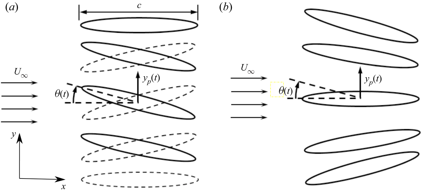
Figure 1. Position of the foil with pitch–plunge flapping kinematics for (a)  $\phi = {\rm \pi}/2$, where the leading edge leads the trailing edge and ‘slices through’ the incoming flow, and (b) $\phi = 2{\rm \pi}$, where the foil appears to be pitching about a point downstream of the trailing edge. The solid lines indicate the upstroke, and the dashed lines indicate the downstroke.
2.2. The immersed boundary method based flow solver
The unsteady flow field is simulated by solving numerically the 2-D incompressible Navier–Stokes equation. A discrete forcing type immersed boundary method (IBM) based in-house flow solver (Majumdar et al. Reference Majumdar, Bose and Sarkar2020a) is used in this study. In the present IBM technique, a ‘momentum forcing’ is applied at all the grid points inside the solid domain. This reconstructs the velocity field in the solid domain in such a way that the appropriate no-slip/no-penetration boundary condition is satisfied exactly on the solid surface (Kim, Kim & Choi Reference Kim, Kim and Choi2001). Moreover, a mass source/sink term is included in the continuity equation to ensure rigorous mass conservation across the immersed boundary. A finite volume based semi-implicit fractional step method (FSM) of  ${\rm \Delta} p$ form is adopted in the present work to advance discretised equations in time. In order to achieve a divergence-free velocity field, a pseudo pressure correction term is used to correct the intermediate velocities at every time step. The convection and diffusion terms are advanced in time using the Adams–Bashforth discretisation and the Crank–Nicolson method, respectively. The spatial derivatives are calculated using the second-order central difference scheme.
The flow Reynolds number is defined as  $Re = {U_{\infty }c}/{\nu }$, with $\nu$ being the kinematic viscosity of the fluid. A flow Reynolds number $Re = 300$ is kept constant for all the simulations of present study. The drag ( $D^{\prime }$) and lift ( $L^{\prime }$) forces on the flapping foil are defined positive along the directions of the positive $x$- and $y$-axes, respectively. The aerodynamic load coefficients are computed as $C_D = {D^{\prime }}/{0.5 \rho _f U_{\infty }^{2} c}$ and $C_L = {L^{\prime }}/{0.5 \rho _f U_{\infty }^{2} c}$, where $\rho _f$ denotes the fluid density.
The flow-governing equations are solved on a background Eulerian grid, with the primitive flow variables ( $u, v, p$) being arranged in a staggered manner. At every time step, the position of the elliptic foil is tracked using $1500$ Lagrangian markers. A rectangular computational domain consisting of a structured non-uniform Cartesian mesh is considered in this study. A uniform grid spacing of ${\rm \Delta} x \times {\rm \Delta} y$ is used in the region of body movement, and then the grid spacing is increased following a geometric progression towards the outer boundaries. The mesh is stretched with common ratio $1.10$ in the upstream direction, and common ratio $1.008$ in the downstream side. In both top and bottom directions, the mesh is stretched with common ratio $1.05$. The boundary conditions are as follows: uniform inflow ( $u = 1, v = 0$), zero-gradient outflow ( $\partial \boldsymbol {u} / \partial x = 0$), and the slip boundary condition ( $\partial u / \partial y = 0$, $v = 0$) at the top and bottom boundaries. Further details on the flow solver can be found in the earlier work by Majumdar et al. (Reference Majumdar, Bose and Sarkar2020a). It was also validated thoroughly in Majumdar et al. (Reference Majumdar, Bose and Sarkar2020a) by comparing the results of the present solver with those available in the literature, and also with the results obtained from a well-established ALE based OpenFOAM solver. The convergence test results relevant to the present study are presented next. Note that the time step size ( ${\rm \Delta} t$), grid spacing ( ${\rm \Delta} x$ and ${\rm \Delta} y$) and domain size reported in the next subsection are in their corresponding non-dimensional forms.
2.3. Convergence tests
For all the convergence test cases, simulations are performed for a simultaneously pitching–plunging elliptic foil with parametric set  $h = 0.375$, $\theta _0 = 15^{\circ }$, $\phi = {\rm \pi}/2$, $\kappa = 4.0$, $x_0 = 0.5$, $t_h/c = 0.12$ and $Re = 300$, which corresponds to a periodic flow field.
2.3.1. Time step convergence test
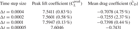
An appropriate time step size has been chosen through a time step independence test with four different time step sizes,  ${\rm \Delta} t = 0.00005$, $0.0001$, $0.0002$ and $0.0004$. The grid size in the uniform mesh region is taken as ${\rm \Delta} x = {\rm \Delta} y = 0.004$, with the mesh stretching ratios towards the outer boundaries being the same as mentioned in § 2.2. The size of the computational domain is considered to be $[-10.0, 30.0]\times [-12.5, 12.5]$ along the $x$- and $y$-axes, respectively. Time histories of $C_D$ and $C_L$ along with close-up views near the peaks, and instantaneous vorticity contours at a typical time instant ( $t/T = 20.25$), are presented in figure 2. Vorticity contour plots are shown considering vorticity range $-10$ to $+10$ throughout the paper. Also, quantitative values of the peak lift coefficient ( $C_L^{peak}$) and average drag coefficient ( $\bar {C}_D$) are presented in table 1 along with the percentage relative difference with respect to the lowest ${\rm \Delta} t$ case considered. Both $C_D$ and $C_L$ time histories, as well as the vorticity contours, for ${\rm \Delta} t = 0.00005$ and $0.0001$ are almost identical. Therefore, ${\rm \Delta} t = 0.0001$ is taken as the appropriate time step size for all the simulations hereafter.
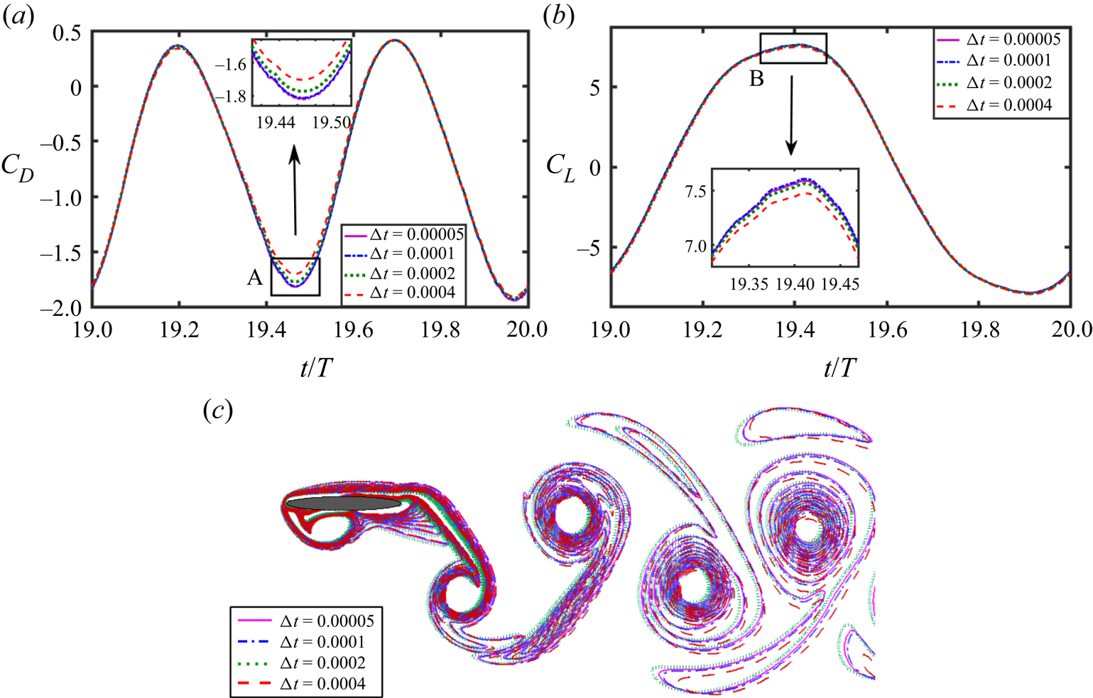
Figure 2. Time step independence test for the flow over a pitching–plunging foil: (a) drag and (b) lift coefficients, and (c) instantaneous vorticity contours at a typical time instant  $t/T = 20.25$.
Table 1. Results of time step convergence study; the values in parentheses denote percentage relative difference with respect to corresponding values of the lowest  ${\rm \Delta} t$ case.
2.3.2. Grid size convergence test
The optimal grid sizes  ${\rm \Delta} x$ and ${\rm \Delta} y$ are also selected based on the outcomes of a grid independence study. To that end, different grid sizes, ${\rm \Delta} x = {\rm \Delta} y = 0.002$, ${\rm \Delta} x = {\rm \Delta} y = 0.004$ and ${\rm \Delta} x = {\rm \Delta} y = 0.008$, have been tested. The ratio of the stretching of the mesh towards the outer boundaries is kept the same, as mentioned in § 2.2, for all of these three different grid sizes. The time step size is taken as ${\rm \Delta} t = 0.0001$, and the computational domain size is $[-10.0, 30.0]\times [-12.5, 12.5]$ along the $x$- and $y$-axes, respectively. The quantitative values of $C_L^{peak}$ and $\bar {C}_D$, and the percentage relative difference with respect to the lowest grid size case, are presented in table 2. The time traces of $C_D$ and $C_L$, as well as the vorticity contours, for grids ${\rm \Delta} x = {\rm \Delta} y = 0.002$ and ${\rm \Delta} x = {\rm \Delta} y = 0.004$ match very closely; see figure 3. Hence the mesh corresponding to grid size ${\rm \Delta} x = {\rm \Delta} y = 0.004$ is chosen for further simulations.
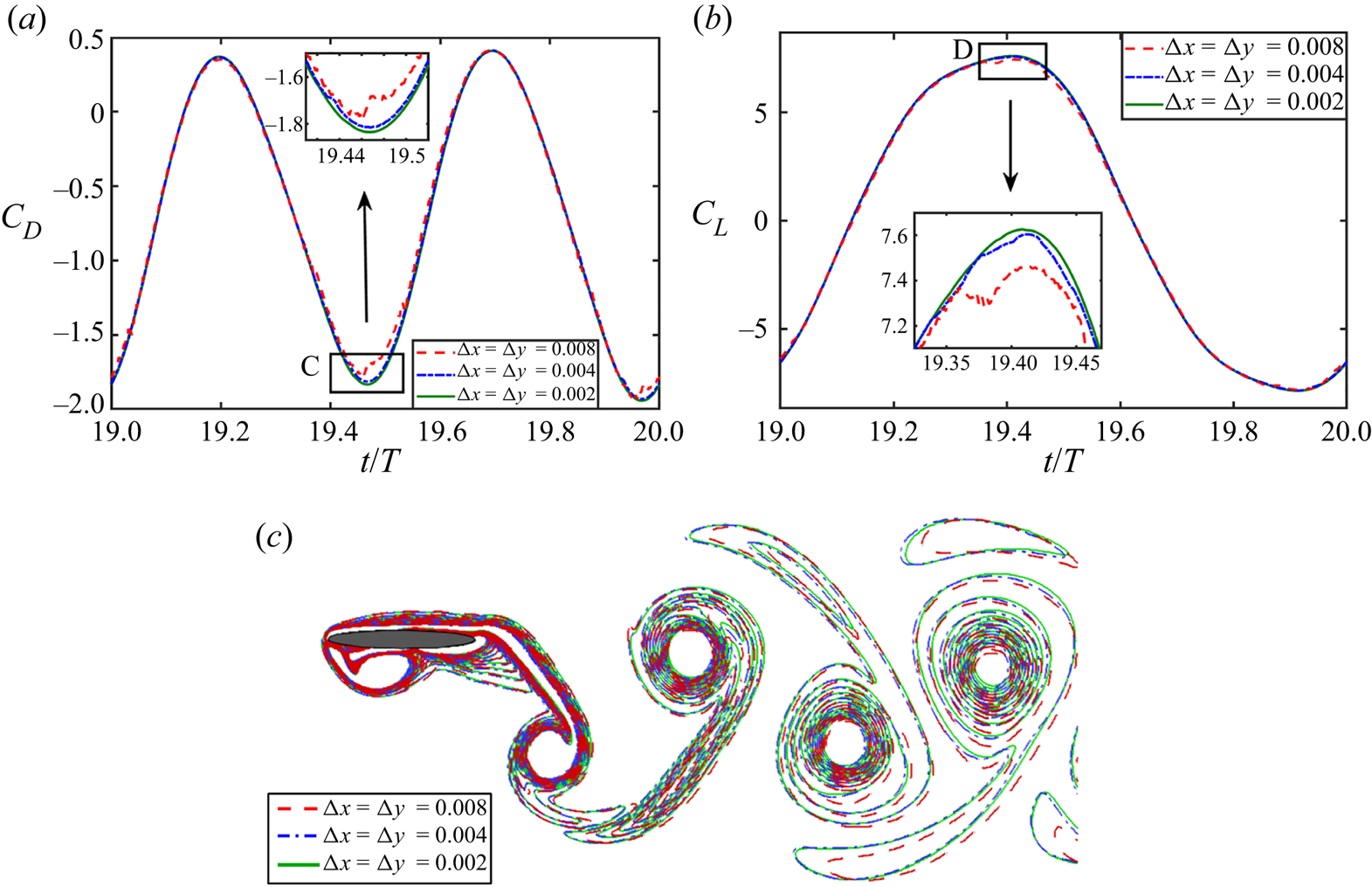
Figure 3. Grid independence test for the flow over a pitching–plunging foil: (a) drag and (b) lift coefficients, and (c) instantaneous vorticity contours at a typical time instant  $t/T = 20.25$.
Table 2. Results of grid-independent study; the values in parentheses denote percentage relative difference with respect to corresponding values of the minimum grid size case.

2.3.3. Domain size convergence test
The size of the computational domain is finalised after performing a domain independence test to ensure that the aerodynamic load coefficients do not change much with further increase in the domain size. Three different rectangular domains are chosen, with sizes as follows: ‘D1’,  $[-5.0, 15.0]\times [-6.25, 6.25]$; ‘D2’, $[-10.0, 30.0]\times [-12.5, 12.5]$; and ‘D3’, $[-20.0, 60.0]\times [-25.0, 25.0]$; with the pitching axis of the foil being placed at the origin at the start of simulations. Time step and minimum grid sizes are taken as ${\rm \Delta} t = 0.0001$ and ${\rm \Delta} x = {\rm \Delta} y = 0.004$, respectively, based on the outcomes of time and mesh convergence tests. Note here that the size of the dense zone and mesh-stretching common ratios are kept the same for all three domains. The $C_L$ and $C_D$ time histories and vorticity contour plot presented in figure 4 show that the results of the medium-sized domain D2 and largest domain D3 are almost identical and do not suffer from boundary effects. The same is evident from the percentage relative difference with respect to the largest domain size case as presented in table 3. Hence D2 is chosen to be the optimum size of the computational domain for all the following simulations.
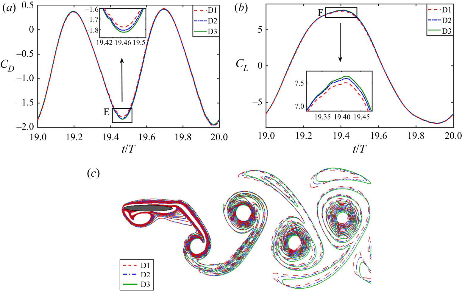
Figure 4. Domain size independence test for the flow over a pitching–plunging foil: (a) drag and (b) lift coefficients, and (c) instantaneous vorticity contours at a typical time instant  $t/T = 20.25$.
Table 3. Results of domain-size-independent study; the values in parentheses denote percentage relative difference with respect to corresponding values of the largest domain size case.

3. Dynamical transitions in the flow field
A wide range of parametric variations has been considered in the present study to investigate their individual and combined effects on the flow field dynamics. This section starts with a description of the parametric space considered here. We also introduce the qualitative/quantitative tools used to distinguish the different nonlinear dynamical states of the flow field, and also demonstrate them for three representative cases of periodic, quasi-periodic and chaotic wakes, the three primary dynamical states encountered in the present study. Subsequently, the flow field behaviour under the entire range of parametric variations is discussed.
3.1. The parametric space
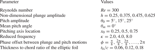
It is known from our earlier studies that periodic-to-chaotic transition happens around  $\kappa h \ge 1.5$ (Badrinath et al. Reference Badrinath, Bose and Sarkar2017; Bose & Sarkar Reference Bose and Sarkar2018; Majumdar et al. Reference Majumdar, Bose and Sarkar2020a; Bose et al. Reference Bose, Gupta and Sarkar2021). However, only the plunge amplitude was varied in those cases, focusing solely on the effects of this single parameter on the system dynamics. In contrast, the present study considers a much wider range of parametric variations for all the relevant key parameters, i.e. plunge amplitude ( $h = 0.25, 0.375, 0.475,0.625$), pitch amplitude ( $\theta _0 = 5^{\circ },15^{\circ },25^{\circ }$), pitching axis location ( $x_0 = 0.25,0.5, 0.75$), flapping frequency ( $\kappa = 2.0,4.0,8.0$) and phase offset (in the range $0 \le \phi \le 2{\rm \pi}$, in steps of ${\rm \pi} /8$). Any of these kinematic parameters can potentially alter the near-field vortex interactions and affect the dynamical transition mechanisms in the flow field. Qualitatively different kinematics (sinusoidal and trapezoidal) are also included here, as well as different foil thickness to chord ratios ( $t_h/c = 0.06, 0.12,0.18$). Throughout the study, the flow Reynolds number is kept constant at $Re = 300$. The overall parametric space is presented in table 4. Results for varying $h$ and $\phi$, with $\theta _0 = 15^{\circ }$, $\kappa = 4.0$, $x_0 = 0.5$ and $t_h/c = 0.12$ being kept fixed, are presented first. The other parameters, i.e. $\theta _0$, $x_0$, $\kappa$ and $t_h/c$, as well as the kinematic pattern, are varied next, one by one, keeping the rest of the parameters unchanged. For these cases, results are presented for plunge amplitude $h = 0.475$ at four typically chosen phase offsets, $\phi = {\rm \pi}/2$, ${\rm \pi}$, $3{\rm \pi} /2$ and $2{\rm \pi}$. The above-mentioned different parametric combinations gave a total of 100 different simulation cases.
Table 4. The parameter space considered in the present study.
3.2. Measures used for dynamical characterisation of the flow field
The wake patterns are classified based on the dynamical characteristics of the unsteady flow field. When the evolution of the vortex structures repeats exactly in consecutive flapping cycles, the corresponding wake is classified as a periodic wake. On the other hand, in the quasi-periodic state, the flow field vortices do not overlap exactly after each cycle; instead, the positions of the vortex cores stay in the close neighbourhood of their previous cycle counterparts. The wake is classified as chaotic when the vortex structures never repeat and the long-term behaviour of the unsteady wake becomes completely unpredictable. These are the three main types of dynamics encountered in the present study. The dynamical states of the flow field at different parametric values are first identified qualitatively through the phase-averaged vorticity plots (Lentink et al. Reference Lentink, Van Heijst, Muijres and Van Leeuwen2010), and subsequently confirmed quantitatively with the help of vorticity correlation values (Bose & Sarkar Reference Bose and Sarkar2018) as well as the phase portraits and the Morlet wavelet transforms (Grossmann, Kronland-Martinet & Morlet Reference Grossmann, Kronland-Martinet and Morlet1990), which are presented in the supplementary material available at https://doi.org/10.1017/jfm.2022.385. Please note that the vorticity correlation coefficient values presented in this study are calculated as an average of the correlation coefficients obtained at the end of  $16$ consecutive flapping cycles (for $t/T = 15.0$ to $t/T = 30.0$). The phase-averaged vorticity plots are also obtained for the same number of flapping cycles. Since the flow field in the periodic regime repeats exactly, the average of the flow field data at the same time instant in several consecutive cycles gives a crisp image of the vorticity contour. But it gives a completely blurry image during chaos when there is no correlation between the flow fields in different cycles. However, the phase-averaged image is neither crisp nor entirely blurry in the quasi-periodic regime. The average vorticity correlation value ( $\rho$), if close to unity, represents periodicity, while it hovers near zero in the chaotic state denoting a near absence of correlation between the flow fields from different cycles. In the quasi-periodic regime, it stays between 0 and 1.
The dynamical characteristics are established further by using a series of other nonlinear time series tools from the dynamical systems theory, such as stroboscopic Poincaré sections (Hilborn et al. Reference Hilborn2000), reconstructed phase portraits (Kennel, Brown & Abarbanel Reference Kennel, Brown and Abarbanel1992) and recurrence plots (Marwan et al. Reference Marwan, Romano, Thiel and Kurths2007). The main advantage of these nonlinear time series tools is that they can establish the nature of the dynamics conclusively even with short time history data. This is particularly useful in our case as simulation of long time histories for many flapping cycles using a high-fidelity Navier–Stokes solver is associated with a prohibitive computational cost. The results obtained using these tools, along with the  $C_L{-}C_D$ phase portraits and Morlet wavelet transforms for three typically chosen parametric cases representative of the periodic, quasi-periodic and chaotic dynamics, are shown in figures 5–7, respectively. Note that these cases are selected randomly as representative cases, and the corresponding parametric values are mentioned in their respective figure captions. A closed loop orbit in the phase portrait diagram indicates a periodic dynamics. Here, the phase space trajectory repeats exactly in different cycles. Hence the stroboscopic Poincaré section converges to a single point (Hilborn et al. Reference Hilborn2000). This is accompanied with an organised narrow frequency band on the wavelet transform plot, and equidistant solid lines parallel to the main diagonal on the recurrence plot. In contrast to periodic dynamics, the trajectory neither repeats exactly nor deviates significantly during the quasi-periodic state, but returns in the neighbourhood of its previous positions, eventually filling the phase space in the form of a toroidal shape, and the Poincaré section depicts a closed loop curve (Hilborn et al. Reference Hilborn2000). The presence of modulating frequency bands along with incommensurate frequencies in the wavelet spectra and unequally spaced lines on the recurrence plot confirms quasi-periodicity. An irregular phase portrait with the Poincaré points being scattered, a broadband frequency spectrum, short and broken diagonal lines along with isolated scattered points on the recurrence plot – all these confirm the existence of chaos in figure 7.
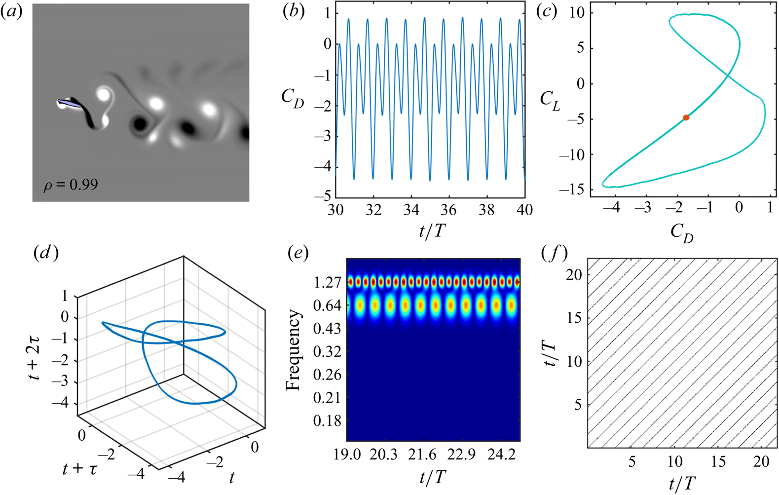
Figure 5. ‘Periodic dynamics’: (a) phase-averaged vorticity contour and average vorticity correlation; (b) time history of drag coefficient; (c)  $C_L{-}C_D$ phase portrait, where the corresponding stroboscopic Poincaré section (red dots) converges to a single point; (d) reconstructed phase portrait of $C_D$, depicting a close loop orbit; (e) organised narrow frequency band in Morlet wavelet transform; and ( f) recurrence plot obtained from the reconstructed $C_D$ data, displaying equidistant solid lines parallel to the main diagonal. All these measures indicate the signature of the periodic flow field. The parametric values are $h = 0.475$, $\theta _0 = 15^{\circ }$, $\phi = 4{\rm \pi} /8$, $\kappa = 4.0$, $x_0 = 0.5$ and $t_h/c = 0.12$.
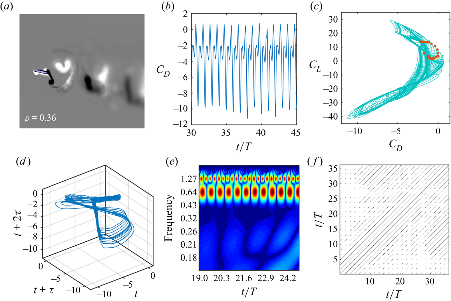
Figure 6. ‘Quasi-periodic dynamics’: (a) phase-averaged vorticity contour and average vorticity correlation; (b) time history of drag coefficient; (c)  $C_L{-}C_D$ phase portrait, where the corresponding stroboscopic Poincaré section (red dots) depicts a close loop; (d) reconstructed phase portrait of $C_D$, depicting a ‘toroidal’ phase portrait; (e) modulating incommensurate frequency band in Morlet wavelet transform; and ( f) recurrence plot obtained from the reconstructed $C_D$ data, displaying unequally spaced lines. All these measures indicate the signature of quasi-periodicity. The parametric values are $h = 0.625$, $\theta _0 = 15^{\circ }$, $\phi = 6{\rm \pi} /8$, $\kappa = 4.0$, $x_0 = 0.5$ and $t_h/c = 0.12$.
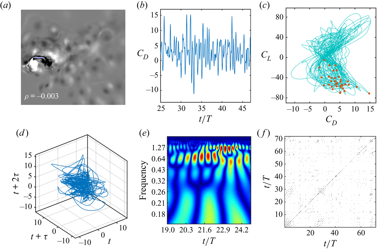
Figure 7. ‘Chaotic dynamics’: (a) phase-averaged vorticity contour and average vorticity correlation; (b) time history of drag coefficient; (c)  $C_L{-}C_D$ phase portrait, where the corresponding stroboscopic Poincaré section (red dots) is scattered; (d) reconstructed phase portrait of $C_D$, depicting a chaotic attractor; (e) broad banded frequency spectra in Morlet wavelet transform; and ( f) recurrence plot obtained from the reconstructed $C_D$ data, displaying short and broken diagonal lines along with isolated scattered points. All these measures indicate the signature of chaos. The parametric values are $h = 0.625$, $\theta _0 = 15^{\circ }$, $\phi = 2{\rm \pi}$, $\kappa = 4.0$, $x_0 = 0.5$ and $t_h/c = 0.12$.
The above discussions demonstrate the way the flow field is classified dynamically in this study. The dynamical transition behaviour in the flow field under different parametric conditions is presented in the next subsection. Only the phase-averaged vorticity contours and the associated average vorticity correlation values are presented here, for the sake of brevity. The  $C_L{-}C_D$ phase portraits and the Morlet wavelet transforms are included in the supplementary material, and they are referred to in the paper in relevant discussions. Results of the other measures for all the 100 different parametric cases are not included here, for the sake of brevity.
3.3. Flow field behaviour under parametric variations
3.3.1. Plunge amplitude ( $h$) and phase offset ($\phi$)


The dynamical transition observed by varying the plunge amplitude and phase offset is shown symbolically in figure 8. Here, each of the data points is marked according to the dynamical signature of the flow field observed in the simulations at those respective parameters. The periodic-to-chaotic transition in the flow field takes place through a quasi-periodic route. For  $\phi = {\rm \pi}$, the flow field is periodic for $h \le 0.375$; it exhibits a quasi-periodic behaviour at $h = 0.475$, and chaos at $\kappa h = 0.625$ (figure 8). Note that with the variation in $\phi$, the onset of the transition along $h$ changes significantly, though the qualitative route remains unchanged. For $2{\rm \pi} /8 \le \phi \le 6{\rm \pi} /8$, the flow field remains periodic even for higher $h$ (
$h$ ( $h = 0.475$) (figure 8), whereas it becomes chaotic even at lower $h$ values ( $h = 0.375$) for $3{\rm \pi} /2 \le \phi \le 2{\rm \pi}$ (figure 8). Thus aperiodic onset gets advanced or delayed depending on the phase offset. This can be attributed to the LEV separation behaviour, which is strongly dependent on $\phi$, as will be discussed in § 4. The flow field results supporting the dynamical transition and the variety in the trailing-wake behaviour are shown in figures 9 and 10. Phase-averaged wake images and average vorticity correlation values are presented for different $\phi$ cases in steps of $2{\rm \pi} /8$.
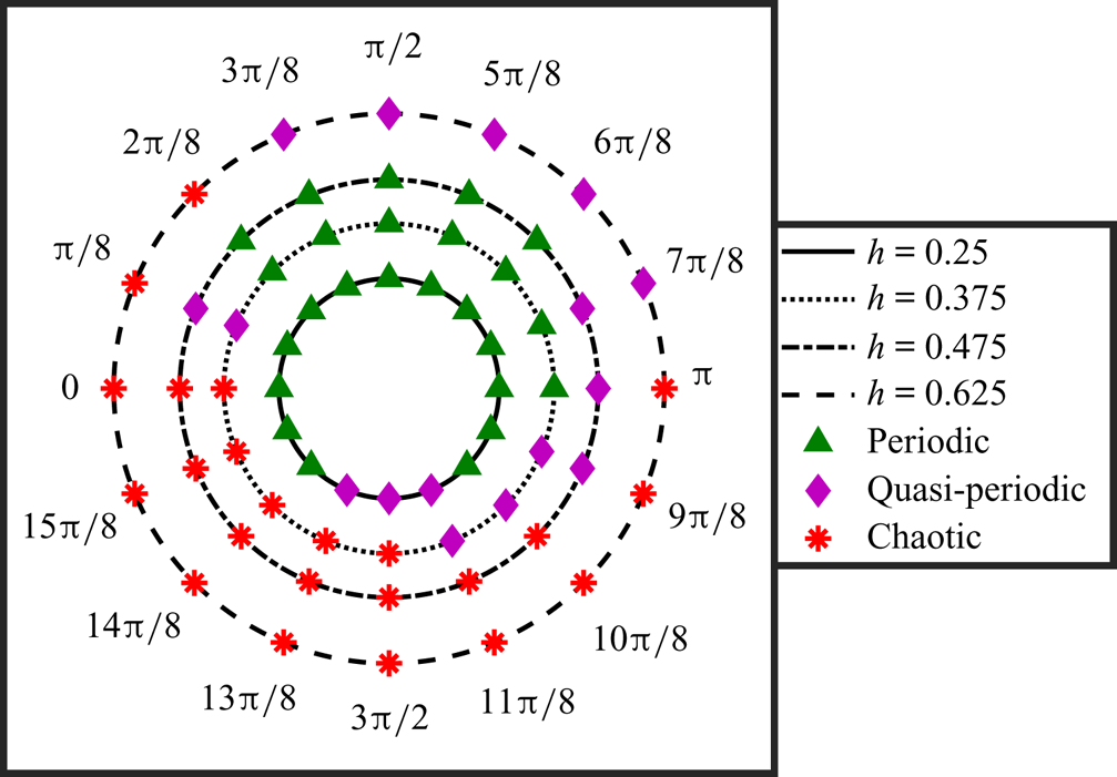
Figure 8. Summarising the dynamical states observed at different  $h$ and $\phi$ values, keeping other parameters fixed.

Figure 9. Phase-averaged vorticity contours at different  $\phi$: (a–h) $h = 0.25$, and (i–p) $h = 0.375$. $\boldsymbol {h = 0.25}$: Figure 8 reveals that for $h = 0.25$, a periodic pattern is shown by the wake for almost all $\phi$ values, except for $11{\rm \pi} /8$ to $13{\rm \pi} /8$, where it turns quasi-periodic. For $h = 0.25$, clockwise (CW) and counter-clockwise (CCW) vortices are seen to shed alternatively in each flapping cycle from the trailing edge. A drag-producing von Kármán wake is observed at $\phi = 2{\rm \pi} /8$ (figure 9a), and a reverse von Kármán wake is seen for $3{\rm \pi} /8 \le \phi \le 10{\rm \pi} /8$. The flow remains completely attached to the body without any LEV formation (figures 9b–e). For $2{\rm \pi} /8 \le \phi \le 10{\rm \pi} /8$, the flow field is periodic and repeats exactly, as revealed by the crisp phase-averaged images. The vorticity correlation remains very close to unity, signifying a strong correlation between the flow fields of different cycles. However, for the $\phi = 12{\rm \pi} /8$ case, the phase-averaged contour is neither crisp nor entirely blurry (figure 9f). The correlation value comes down to $0.74$, indicating a quasi-periodic flow signature. The flow field returns to periodicity at $14{\rm \pi} /8 \le \phi \le 2{\rm \pi}$ (figures 9g,h). The $C_L{-}C_D$ phase portraits and the wavelet spectra of all the above cases are presented, respectively, in figures 1(a–h) and 3(a–h) of the supplementary material. $\boldsymbol {h = 0.375}$: For $\phi = 2{\rm \pi} /8$, the von Kármán wake of $h = 0.25$ turns into reverse von Kármán at $h = 0.375$ (figure 9i). The wake undergoes deflection during $4{\rm \pi} /8 \le \phi \le 10{\rm \pi} /8$, and the deflection angle increases with the increase in $\phi$; see figures 9(j–m). The flow remains periodic in the range $2{\rm \pi} /8 \le \phi \le 8{\rm \pi} /8$, but shows quasi-periodic signatures at $\phi = 10{\rm \pi} /8$ with $\rho = 0.85$. The flow field exhibits chaos for $12{\rm \pi} /8 \le \phi \le 2{\rm \pi}$, where the flow is irregular and the long-term behaviour is unpredictable. Chaos is confirmed by the correlation values being close to zero, and also the entirely blurry patterns seen in figures 9(n–p). The phase portrait and wavelet plots corresponding to the cases of figures 9(i–p) are presented in figures 1(i–p) and 3(i–p) of the supplementary material, respectively, and support the dynamical characteristics observed in the flow field plots. $\boldsymbol {h = 0.475}$: At this $h$, the trailing wake exhibits several interesting flow patterns for varying $\phi$. A deflected reverse von Kármán wake is seen at $\phi = 2{\rm \pi} /8$ (figure 10a), with CW and CCW vortices shed in alternate fashion at every cycle. An S + P pattern (Williamson & Roshko Reference Williamson and Roshko1988) is seen at $\phi = 4{\rm \pi} /8$ (figure 10b) with a single CCW vortex (S) and a pair of CW and CCW vortices (P) shed in every cycle. For the latter, the CCW part of P gets shredded (Gustafson & Leben Reference Gustafson and Leben1988) gradually under the influence of its stronger CW partner, and the far wake transforms to a downward deflected reverse von Kármán wake. The deflection direction gets reversed as $\phi$ crosses ${\rm \pi} /2$, giving an upward deflected wake at $\phi = 6{\rm \pi} /8$ (figure 10c). This is because the initial direction of the pitch rotation gets reversed as $\phi$ crosses ${\rm \pi} /2$, influencing the direction of deflection (Zheng & Wei Reference Zheng and Wei2012; Majumdar, Bose & Sarkar Reference Majumdar, Bose and Sarkar2020b). Although the wake patterns vary with $\phi$, they remain periodic within $2{\rm \pi} /8 \le \phi \le 6{\rm \pi} /8$, and turn quasi-periodic at $\phi = 8{\rm \pi} /8$ (figure 10d). Finally, the flow field becomes chaotic for $10{\rm \pi} /8 \le \phi \le 2{\rm \pi}$ as denoted by the entirely blurry phase-averaged patterns and almost zero vorticity correlation; see figures 10(e–h). Figures 2(a–h) and 4(a–h) of the supplementary material present the phase portrait and wavelet plots corresponding to the cases of figures 10(a–h), respectively.
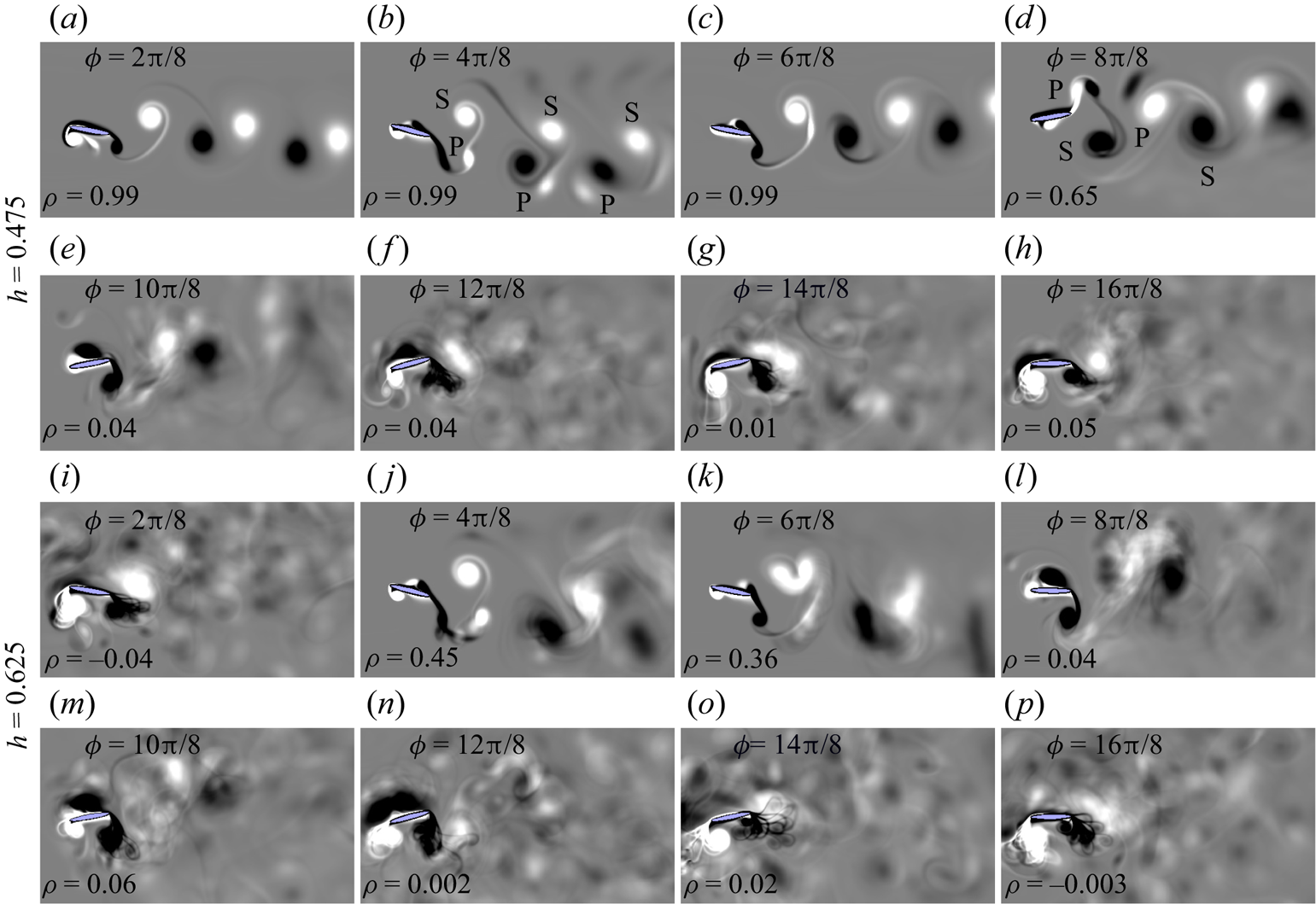
Figure 10. Phase-averaged vorticity contours at different  $\phi$; (a–h) $h = 0.475$, and (i–p) $h = 0.625$. $\boldsymbol {h = 0.625}$: At this high plunge amplitude, the organised pattern of the wake is almost entirely lost, and chaos is seen for a wide range of $\phi$ ( $0 \le \phi \le 2{\rm \pi} /8$ and ${\rm \pi} \le \phi \le 2{\rm \pi}$); see figures 10(i,l–p). Outside this regime ( $3{\rm \pi} /8 \le \phi \le 7{\rm \pi} /8$), quasi-periodic flow signatures are observed (figures 10j,k). These claims are confirmed further by the $C_L{-}C_D$ phase portraits and wavelet spectra presented in figures 2(i–p) and 4(i–p) of the supplementary material.
3.3.2. Pitch amplitude, $\theta _0$

The pitch amplitude is varied as  $\theta _0 = 5^{\circ }$, $15^{\circ }$ and $25^{\circ }$. Other kinematic parameters are kept fixed at $h = 0.475$, $\kappa = 4.0$, $x_0 = 0.5$ and $t_h/c = 0.12$. Figure 11 presents the dynamical states corresponding to these parametric cases, and the identified dynamical signatures are further confirmed by $C_L{-}C_D$ phase plots and wavelet spectra presented in figures 5 and 6 of the supplementary material. For $\theta _0 = 15^{\circ }$ and $25^{\circ }$, the transition route remains the same, i.e. periodic at $\phi = {\rm \pi}/2$, quasi-periodic at $\phi = {\rm \pi}$, and chaos at $\phi = 3{\rm \pi} /2$ and $2{\rm \pi}$. At $\theta _0 = 5^{\circ }$, the effect of the pitch motion is comparatively lesser, with the flow field getting dictated primarily by the dominant plunge motion. For this $\theta _0$, the periodic flow field is absent at the chosen $\phi$ values; quasi-periodic flow is seen for $\phi = {\rm \pi}/2$, ${\rm \pi}$ and $2{\rm \pi}$; and robust chaos is exhibited at $\phi = 3{\rm \pi} /2$.
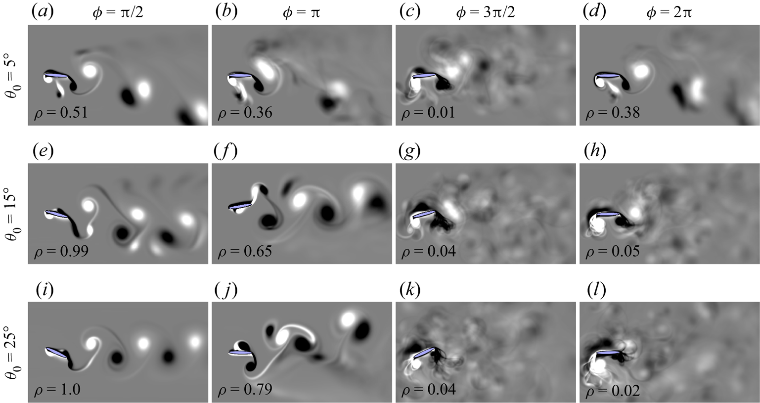
Figure 11. Phase-averaged vorticity contours for different pitch amplitudes and phase offsets at  $h = 0.475$, $\kappa = 4.0$, $x_0 = 0.5$ and $t_h/c = 0.12$.
3.3.3. Location of the pitching axis, $x_0$

To investigate the effect of different pitching axis locations, three different pivot points have been chosen,  $x_0 = 0.25$, $0.5$ and $0.75$, i.e. at the quarter-chord, mid-chord and three-quarter-chord, respectively. All other parameters are kept fixed at $h = 0.475$, $\theta _0 = 15^{\circ }$, $\kappa = 4.0$ and $t_h/c = 0.12$. The resulting flow field dynamics are demonstrated in figure 12. The corresponding $C_L{-}C_D$ phase portraits and wavelet transforms of $C_D$ time histories are presented in figures 7 and 8 of the supplementary material, respectively. It is evident from these results that the dynamical states are not drastically different for different pitching axis locations. The influence of pivot location on the dynamical characteristics is insignificant at $\phi = {\rm \pi}/2$ and $3{\rm \pi} /2$. The flow field displays periodicity at $\phi = {\rm \pi}/2$, and chaos at $\phi = 3{\rm \pi} /2$. However at $\phi = {\rm \pi}$, there is gradual change in the dynamical signature, showing quasi-periodicity for $x_0 = 0.25$ and $x_0 = 0.5$, but purely periodic behaviour at $x_0 = 0.75$. This indicates that the flow field gets regularised gradually as the pivot location is moved towards the trailing edge at $\phi = {\rm \pi}$. This can be noticed from the gradual increase in the average vorticity correlation values at $\phi = {\rm \pi}$ ( $\rho = 0.40$, $0.65$ and $0.98$ at $x_0 = 0.25$, $0.5$ and $0.75$, respectively); see figure 12. On the other hand, at $\phi = 2{\rm \pi}$, despite all three $x_0$ cases being chaotic, an increase in the degree of irregularity can be noticed from the decrease in the magnitude of average vorticity correlation values as $x_0$ increases ( $\lvert \rho \lvert = 0.15$, $0.05$ and $0.02$ at $x_0 = 0.25$, $0.5$ and $0.75$, respectively); see figure 12. In conclusion, as the pivot point is moved from the leading edge towards the trailing edge, the flow field gets regularised at $\phi = {\rm \pi}$, but becomes more and more irregular at $\phi = 2{\rm \pi}$. The physical reason behind this trend is presented in Appendix C, as this can be appreciated better after the discussion on the role of flapping motion on LEV growth, and in turn, on the dynamical states, as given in §§ 4 and 5.1.
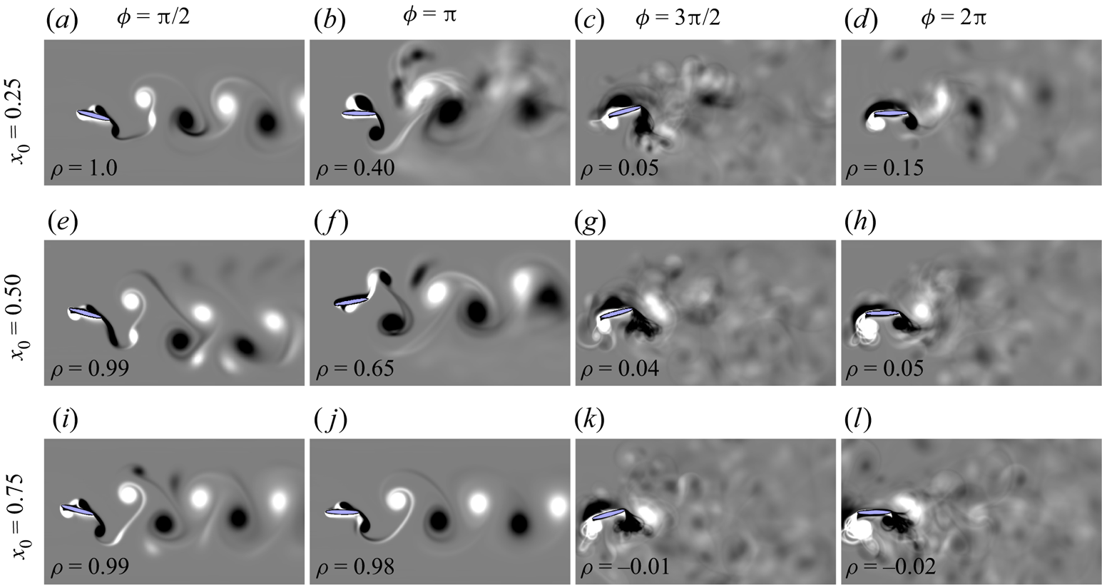
Figure 12. Phase-averaged vorticity contours for different pitching axis locations and phase offsets at  $h = 0.475$, $\theta _0 = 15^{\circ }$, $\kappa = 4.0$ and $t_h/c = 0.12$.
3.3.4. Flapping frequency, $\kappa$

In this case, we have chosen two new flapping frequencies,  $\kappa = 2.0$ and $8.0$, i.e. half of and double the earlier chosen frequency. Other kinematic parameters are kept fixed at $h = 0.475$, $\theta _0 = 15^{\circ }$, $x_0 = 0.5$ and $t_h/c = 0.12$. The phase-averaged vorticity contour plots are presented in figure 13. Figures 9 and 10 of the supplementary material present the corresponding $C_L{-}C_D$ phase plots and the wavelet spectra, respectively. For $\kappa = 2.0$, the resultant dynamical flapping velocity is so low that the flow exhibits a periodic dynamic independent of the phase offset value between pitch and plunge motions. On the other hand, at $\kappa = 8.0$, the flapping velocity being significantly high, the flow field exhibits chaos at all $\phi$ values. Thus the flapping frequency can be a control parameter to trigger a periodic to chaotic transition in the wake.
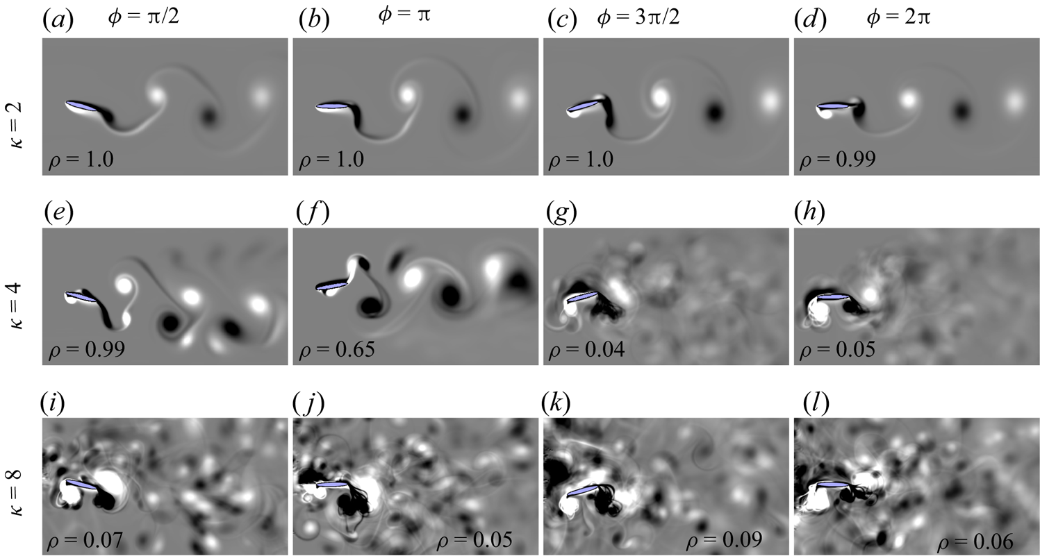
Figure 13. Phase-averaged vorticity contours for different flapping frequencies and phase offsets at  $h = 0.475$, $\theta _0 = 15^{\circ }$, $x_0 = 0.5$ and $t_h/c = 0.12$.
3.3.5. Thickness to chord ratio of the foil, $t_h/c$

The simulations are run for different foil thicknesses with three different thickness to chord ratios,  $t_h/c = 0.06$, $0.12$ and $0.18$, respectively, keeping the kinematic parameters constant at $h = 0.475$, $\theta _0 = 15^{\circ }$, $\kappa = 2.0$ and $x_0 = 0.5$. The phase-averaged vorticity contours shown in figure 14 display clearly that the dynamical states for the three chosen foil thicknesses remain almost the same – periodic at $\phi = {\rm \pi}/2$, quasi-periodic at ${\rm \pi}$ and chaotic at $3{\rm \pi} /2$, respectively. However, a minor difference is observed at $\phi = 2{\rm \pi}$, where $t_h/c = 0.06$ and $t_h/c = 0.12$ result in chaos, while the thicker foil with $t_h/c = 0.18$ exhibits quasi-periodicity. Though the flow dynamics is quasi-periodic at $t_h/c = 0.18$, the average correlation of the vorticity field remains on the lower side ( $\rho = 0.23$). This signifies that the system at this parametric situation is very close to chaos, and any small change in the parameters may push it to robust chaos. It can be concluded here that the foil shape does not play a crucial role behind transition under the chosen parametric conditions. The dynamical characteristics remain more or less similar irrespective of the change in the thickness or shape, provided that the foil is not significantly thick ( $t_h/c = 0.18$ or greater based on the observations of the present study).

Figure 14. Phase-averaged vorticity contours for different foil thicknesses and phase offsets at  $h = 0.475$, $\theta _0 = 15^{\circ }$, $\kappa = 4.0$ and $x_0 = 0.5$.
3.3.6. Flapping profile
The discussion so far has been based entirely on pure sinusoidal kinematics, and will be referred to as ‘Flapping I’ hereafter. In this section, another variety of flapping motion pattern is tested, namely a sinusoidal plunge along with a trapezoidal pitch motion, and this will be referred to as ‘Flapping II’ in this study. The kinematics is given by
 $$\begin{gather} y_p(t)=h_0 \sin(2 {\rm \pi}f_e t), \end{gather}$$
 $$\begin{gather}\theta(t)= \theta_m + \frac{\theta_0}{\tanh \beta} \tanh ( \beta \sin(2 {\rm \pi}f_e t + \phi)), \end{gather}$$
where  $\beta$ is a scaling parameter to match the amplitudes, taken as $\beta = 2.5$ in this study.
The kinematic parameters are taken as  $h = 0.475$, $\theta _0 = 15^{\circ }$, $\kappa = 4.0$, $x_0 = 0.5$ and $t_h/c = 0.12$. Once again, four different $\phi$ values are chosen, $\phi = {\rm \pi}/2$, ${\rm \pi}$, $3{\rm \pi} /2$ and $2{\rm \pi}$. Figure 15 shows the flapping patterns for $\phi = {\rm \pi}/2$ and $2{\rm \pi}$. The dynamical states of the flow fields are presented in figure 16; the $C_L{-}C_D$ plots and wavelet transforms are given in figures 13 and 14 of the supplementary material. It is seen that the transition route remains the same for both Flapping I and Flapping II, exhibiting periodicity at $\phi = {\rm \pi}/2$, quasi-periodicity at $\phi = {\rm \pi}$, and chaos at $\phi = 3{\rm \pi} /2$ and $2{\rm \pi}$. This indicates that small changes in the flapping pattern do not affect the dynamical transition behaviour much.
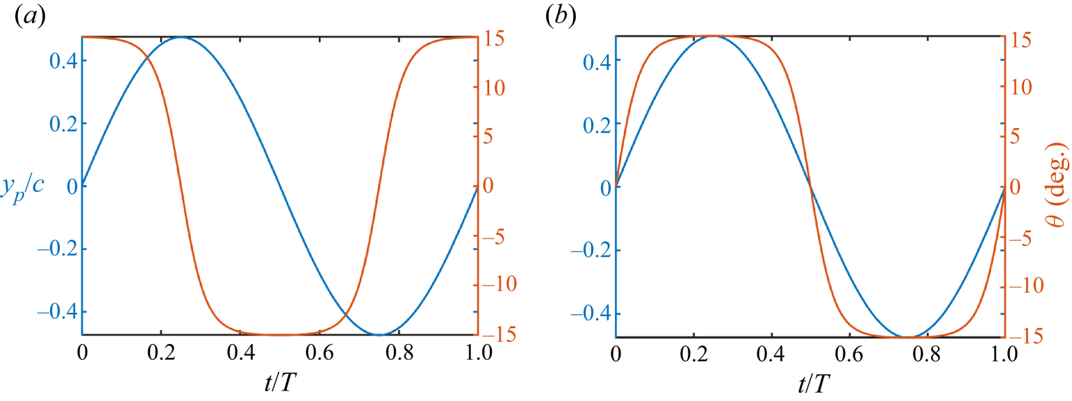
Figure 15. Flapping pattern considering sinusoidal plunge along with trapezoidal pitch motion: (a)  $\phi = {\rm \pi}/2$, and (b) $\phi = 2{\rm \pi}$.
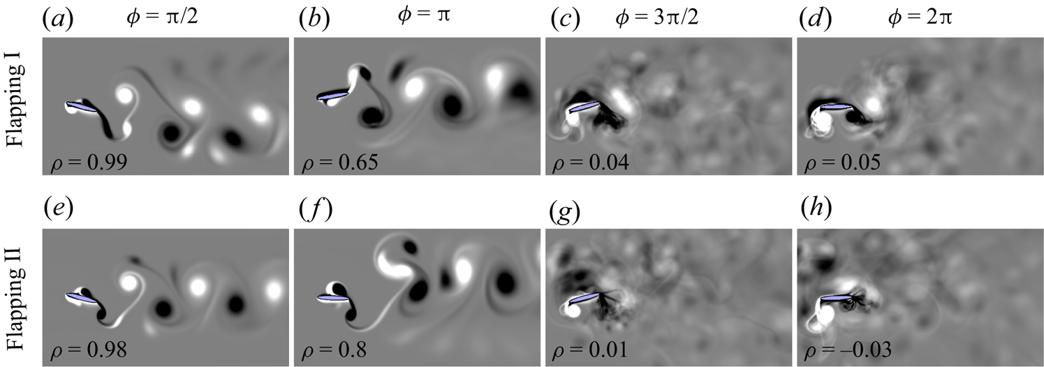
Figure 16. Phase-averaged vorticity contours for different flapping patterns and phase offsets at  $h = 0.475$, $\theta _0 = 15^{\circ }$, $\kappa = 4.0$, $x_0 = 0.5$ and $t_h/c = 0.12$. Flapping I: sinusoidal plunge and sinusoidal pitch. Flapping II: sinusoidal plunge and trapezoidal pitch.
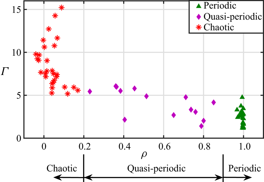
Figure 17. Average circulation of the primary LEV shows strong correlation with the periodicity of the flow field.
With the knowledge of the dynamics from these 100 different simulation cases, the role of the key vortex structures, especially the LEV, in triggering aperiodicity in the wake is investigated next. A correlation between the strength of the LEV and the dynamical state of the wake is also sought.
4. Role of the primary LEV on flow field periodicity
The primary LEV is one of the key near-field structures to dictate the dynamical state of the flow field. As mentioned in the Introduction, LEV growth and separation become aperiodic in the high  $\kappa h$ regime, and the subsequent LEV–TEV interactions lead to spontaneous formation and destruction of series of secondary vortices, thus triggering aperiodicity in the wake (Bose & Sarkar Reference Bose and Sarkar2018; Majumdar et al. Reference Majumdar, Bose and Sarkar2020a; Bose et al. Reference Bose, Gupta and Sarkar2021). The strong interconnection between LEV growth and the chaotic transition of the flow field is demonstrated quantitatively in the present study in terms of the strength of the LEV. Figure 17 shows the variation in the average LEV strength ( $\varGamma$) at different parametric cases, along with the associated $\rho$ values, presented in § 3.3. In order to estimate the LEV strengths, circulation values are calculated as an integral of the vorticity field over a rectangular region that covers the LEV area around the location of maximum vorticity (Zurman-Nasution et al. Reference Zurman-Nasution, Ganapathisubramani and Weymouth2020). The position and size of the rectangular box are changed depending on the location and size of the primary LEV at different time instants and different parameters. Some examples of such rectangular regions surrounding the LEV can be seen in figure 18 for a few typical flow field snapshots. The integration is performed at a time instant when the foil completes an upstroke and reaches its topmost position. The primary counter-clockwise LEV is assumed to be fully grown at this instant. The LEV circulation is obtained for 16 consecutive flapping cycles ( $t/T = 15\unicode{x2013}30$), and the average LEV strength, $\varGamma$, is computed. From the $\varGamma$ versus $\rho$ plot in figure 17, a direct correlation between the strength of the primary LEV and the chaotic transition in the flow field can be observed. For the periodic cases, in general, $\varGamma$ is seen to remain bounded (approximately $\varGamma < 5$). In the majority of these cases, the LEV, being weak in strength, does not get shed and remains attached to the body. As a result, no LEV–TEV interactions take place in the near field. For the quasi-periodic cases, $\varGamma$ is seen to cover almost the same range as that of the periodic cases (approximately $1.5 < \varGamma < 6$). So periodic and quasi-periodic dynamics cannot be distinguished clearly based on the $\varGamma$ values alone. On the other hand, for most of the chaotic cases, $\varGamma$ goes beyond a certain threshold, approximately at $\varGamma > 6$; see figure 17. This indicates that beyond a certain strength, the growth of the LEV turns chaotic, triggering the entire flow field to be chaotic eventually. Notably large variations in the circulation values at different cycles are seen during chaos, and a high average is observed. A strong LEV is shed from the body during different flapping cycles aperiodically, and subsequently interacts with the TEV to propagate chaos in the wake.

Figure 18. Comparison of the instantaneous vorticity contours at  $t/T = 20.25$ (at the end of an upstroke) for $h = 0.25, 0.375, 0.475,0.625$ at four typically chosen phase offset values ( $\phi = {\rm \pi}/2, {\rm \pi}, 3{\rm \pi} /2,2{\rm \pi}$). The circulation of the primary LEV is mentioned in each panel. The black rectangular boxes show the region considered to calculate the circulation values. SV: secondary vortex.
The fundamental mechanisms that dictate the onset of chaotic transition are related to the LEV and other near-field vortices, as will be shown next. They are examined in this section based on a few typically chosen representative cases. A comparison of the near-field vortices at four  $h$ values ( $0.25, 0.375, 0.475,0.625$) is presented in figure 18 for four typical $\phi$ cases ( ${\rm \pi} /2, {\rm \pi}, 3{\rm \pi} /2,2{\rm \pi}$). These representative cases are taken from § 3.3.1. Note that the circulation values shown in the panels of figure 18 correspond to each specific snapshot, and are not the averaged quantities. For a better appreciation of the foil motion, the orientations of the foil at different time instants during a flapping cycle are shown schematically in figure 19, corresponding to the cases presented in figure 18. These pictorial representations will be useful in the follow-up discussion. The effective AoA $\alpha _{eff}$ is also computed for each of these cases using the equation
 \begin{equation} \alpha_{eff}(t) = \theta(t) - \tan^{{-}1} \left[\frac{1}{U_{\infty}} \left\{ \dot{y}_p(t) - \left(\frac{c}{2} - x_0 \right) \dot{\theta}(t) \cos(\theta(t)) \right\} \right]. \end{equation}
The derivation of this equation is given in Appendix A. The numerical value of  $\alpha _{eff}$ depends on both the plunge and pitch parameters, as well as on the phase offset between them. Figure 20 presents $\alpha _{eff}$ over a flapping cycle for a typical case with $h = 0.475$ at four different $\phi$ values. The trend remains the same for the other $h$ values. The $\alpha _{eff}$ values reported in the following discussion are specific to the $h = 0.475$ case.
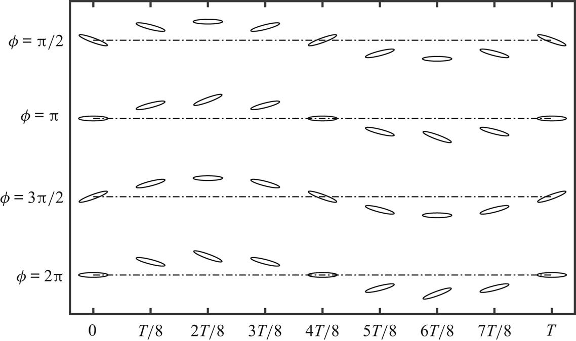
Figure 19. Schematic diagram showing the pitching–plunging foil motion at  $\phi = \frac {{\rm \pi} }{2}, {\rm \pi}, \frac {3{\rm \pi} }{2}$ and $2{\rm \pi}$.
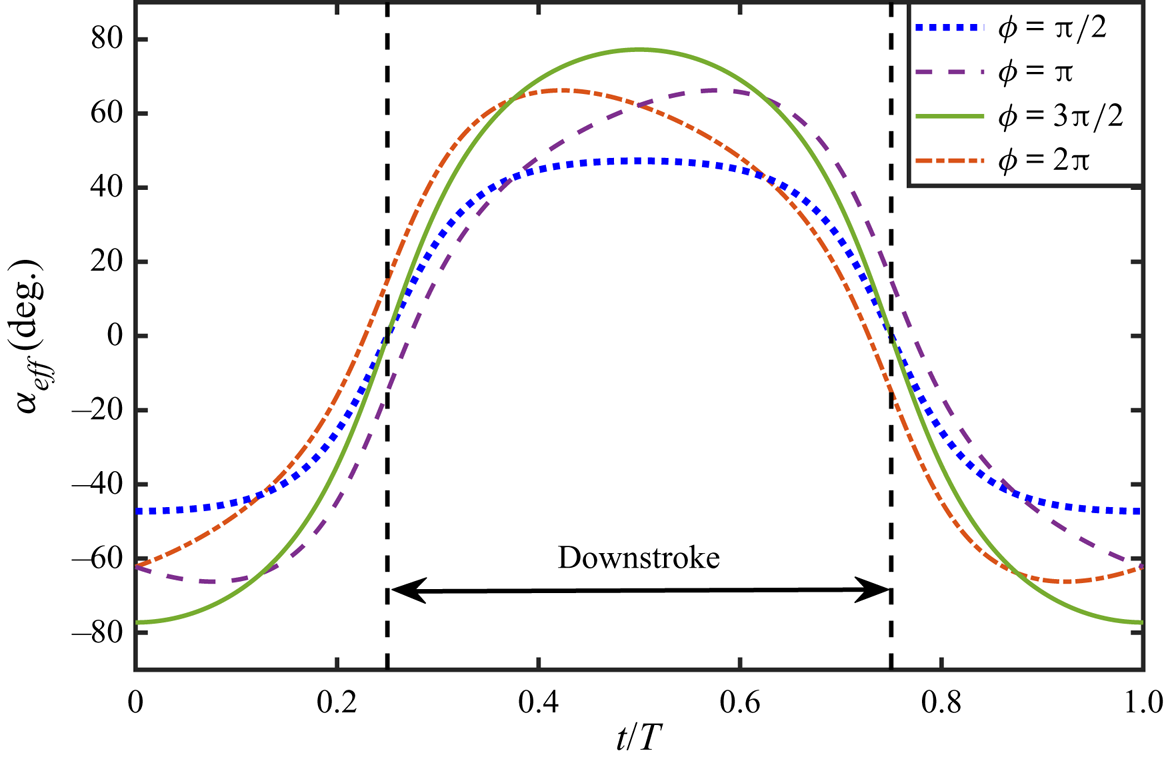
Figure 20. Effective AoA for a typical case  $h = 0.475$ at four different $\phi$ values. The trend remains the same at the other $h$ values.
The phase offset between the plunge and pitch motions is a crucial parameter in ultimately dictating the relative orientation of the flapping foil with respect to the incoming flow. At  $\phi = {\rm \pi}/2$, the leading edge of the foil leads the trailing edge, and the foil ‘slices through’ the free stream (see figure 19), thus minimising the maximum value that the effective AoA can reach ( $\alpha _{eff}^{max} = 47.24^{\circ }$ for $h = 0.475$, see figure 20). As a result, the flow remains completely attached to the body at $h = 0.25$ (figure 18a). Even though an LEV forms with an increase in $h$, the circulation of the LEV remains low ( $\varGamma = 1.82$ at $h = 0.375$, and $\varGamma = 3.73$ at $h = 0.475$), and it stays attached to the body. No strong LEV separation is seen. The LEV does not undergo any direct interaction with the TEV; see figures 18(b,c). Thus for $\phi = {\rm \pi}/2$, the flow field exhibits periodic vortex shedding even at $h = 0.475$. The periodic formation and growth of the primary LEV becomes quasi-periodic only at a significantly high $h=0.625$, when the circulation of the primary LEV also increases to $\varGamma = 6.47$.
As  $\phi$ goes to ${\rm \pi}$, the flow still remains attached at $h = 0.25$, and periodic vortex shedding is seen at the trailing edge (figure 18e). With an increase in $h$, an LEV forms as seen in figures 18( f–h). At this $\phi$, although the maximum effective AoA is high ( $\alpha _{eff}^{max} = 66.24^{\circ }$ for $h = 0.475$, as in figure 20), the leading edge traverses the smallest distance. Hence the LEV does not get separated from the body. However, it gradually gets convected along the foil surface to affect the TEV shedding. As the LEV growth becomes aperiodic around $h \ge 0.475$, it triggers the entire near-field interactions to be aperiodic.
At  $\phi = 3{\rm \pi} /2$, the kinematics being exactly the mirror image of those for $\phi = {\rm \pi}/2$, the leading edge lags the trailing edge (figure 19), and $\alpha _{eff}^{max}$ takes the highest value among all the other $\phi$ cases ( $\alpha _{eff}^{max} = 77.24^{\circ }$ for $h = 0.475$, see figure 20). As a result, strong separation happens near the leading edge (figures 18i–l) and it becomes aperiodic even near $h = 0.25$. The aperiodically shed LEV (with $\varGamma = 5.75$ at $h = 0.375$, $\varGamma = 4.49$ at $h = 0.475$, and $\varGamma = 14.98$ at $h = 0.625$), interacts with the TEV to trigger chaos. Consequently, spontaneous formation and annihilation of vortices through some of the fundamental interaction mechanisms sustains chaos in the far wake. Such interaction mechanisms were discussed in detail by Bose & Sarkar (Reference Bose and Sarkar2018) and Majumdar et al. (Reference Majumdar, Bose and Sarkar2020a).
At  $\phi = 2{\rm \pi}$, plunge and pitch are in the same phase, and the leading edge traverses the largest distance, giving a high maximum effective AoA ( $\alpha _{eff}^{max} = 66.24^{\circ }$ for $h = 0.475$, see figure 20). A strong LEV gets separated even at low $h$, but with high LEV strength. This can be seen from figures 18(n–p) ( $\varGamma = 2.71$ at $h = 0.25$, $\varGamma = 4.69$ at $h = 0.375$, $\varGamma = 7.43$ at $h = 0.475$, and $\varGamma = 9.17$ at $h = 0.625$). Once again, subsequent interactions with the TEV usher in and sustain chaos.
The above discussion underlines the importance of the foil orientation in affecting the growth and evolution of the primary LEV and in dictating its subsequent interactions with the other vortices. Parameters such as the phase offset can influence this strongly. One can state from the above results that the  $\phi = {\rm \pi}/2$ case should be preferred for a delayed onset of chaos as it ensures no strong separation and an organised flow for a longer range of $h$. Similarly, $3{\rm \pi} /2 \le \phi \le 2{\rm \pi}$ should be avoided as the aperiodic onset gets advanced due to the formation and shedding of strong aperiodic leading-edge vortices, even at low $h$.
$h$.
At this juncture, it is important to identify new non-dimensional parameters that can capture robustly the combined effects of the key kinematics on the LEV separation behaviour discussed above. These novel non-dimensional parameters are to be utilised to demarcate the different dynamical states of the wake without any loss of generality. With this focus, the next section identifies two new non-dimensional parameters and proposes a mathematical fit in terms of them to isolate the order-to-chaos transition region and classify the dynamical states.
5. Dynamical transition boundaries and an order-to-chaos map
As already mentioned, none of the conventionally used existing non-dimensional parameters ( $\kappa h$, $St_A$, $St_D$, $St_c$, $St_{\tau }$) can account for the combined effect of many different kinematic quantities. The limitations of the earlier approaches using existing non-dimensional parameters in demarcating different dynamical regimes are presented in Appendix B. We remind readers that the current study considers a wide variety of parametric combinations, some of which are being discussed for the first time. This brings out the need for developing new non-dimensional quantities that can capture effectively the effects of varying all the relevant kinematic parameters on the flow field. This is presented in the following. Generalised order-to-chaos transition boundaries are also identified in the present study in terms of the proposed non-dimensional quantities.
5.1. Introducing new non-dimensional quantities to capture the dynamics
As already demonstrated, the dynamical signature of the flow field is dictated primarily by the LEV separation. This, in turn, is dependent on the flapping kinematics as well as the inflow, i.e. the speed and relative orientation with which the leading edge interacts with the incoming flow. The effective AoA should be a powerful measure in this regard to define the degree of the flow separation. A novel and efficient mathematical model is proposed here to represent the entire parametric space in terms of the maximum effective AoA in one cycle ( $\alpha _{eff}^{max}$) and a leading-edge amplitude-based Strouhal number ( $St_{A,LE}$). The latter is defined as
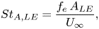 \begin{equation} St_{A,LE} = \frac{f_e\,A_{LE}}{U_{\infty}}, \end{equation}
with  $A_{LE}$ denoting the peak-to-peak amplitude of the leading edge. It can be estimated as
 \begin{equation} A_{LE} =2 \times \max\{ y_p(t) + x_0 \sin(\theta(t)) \}. \end{equation}
These two key non-dimensional parameters,  $\alpha _{eff}^{max}$ and $St_{A,LE}$, are able to include both of the critical aspects discussed above – the speed and the angle with which the foil interacts with the inflow. The mathematical definitions of these two quantities include the effects of all the key kinematic and flow parameters that affect the wake dynamics. Thus changes in any of these parameters reflect directly on the $\alpha _{eff}^{max}$– $St_{A,LE}$ pair, which is not true for the conventionally used non-dimensional numbers defined for specific kinematic situations.
As a first step, the  $(St_{A,LE}, \alpha _{eff}^{max})$ pair values corresponding to all the parametric cases presented in § 3, exhibiting periodic or chaotic dynamics, are computed and plotted in the $\alpha _{eff}^{max}$ versus $St_{A,LE}$ plane. It is observed that the data points belonging to the periodic and chaotic states are clustered individually in two distinct regions; see figure 21. A best fit curve $\alpha _{eff}^{max} = 61.1\,St_{A,LE}^{-0.22}$ is obtained from the boundary data of the chaotic cases using a power-law equation. This is considered as the lower boundary of the chaotic regime since all the data points belonging to the region above this curve are representative of robust chaos. Similarly, another best fit curve, $\alpha _{eff}^{max} = 45.8\,St_{A,LE}^{-0.2}$, is obtained from the boundary data of the periodic points, and all the data points below this curve belong to the periodic regime. Thus the latter curve can be considered as the upper boundary of the periodic regime. The philosophy behind the development of these two boundaries is based on the motivation of identifying the loss of periodicity and the onset of chaos. Interestingly, all the parametric data exhibiting quasi-periodicity (transition state) in § 3 fall in the region bounded by the two above-mentioned boundary curves. Even though these boundaries are developed from the information of periodic and chaotic data points alone, the quasi-periodic points turn out to be well segregated and bounded by them. Therefore, the $\alpha _{eff}^{max}$ versus $St_{A,LE}$ plot in figure 21 captures efficiently the three distinct dynamical regimes, where the periodic and chaotic regimes are separated by the transitional quasi-periodic regime. It is also worth mentioning that the choice of power-law curves here is a methodological choice. Several other standard fittings were tried out as well, but the power-law fitting gave the highest accuracy. However, the exponent values in the power-law curves, i.e. $-0.2$ for the upper bound of the periodic cases, and $-0.22$ for the lower bound of the chaotic cases, are not by choice but are outcomes of the best-fitting process.
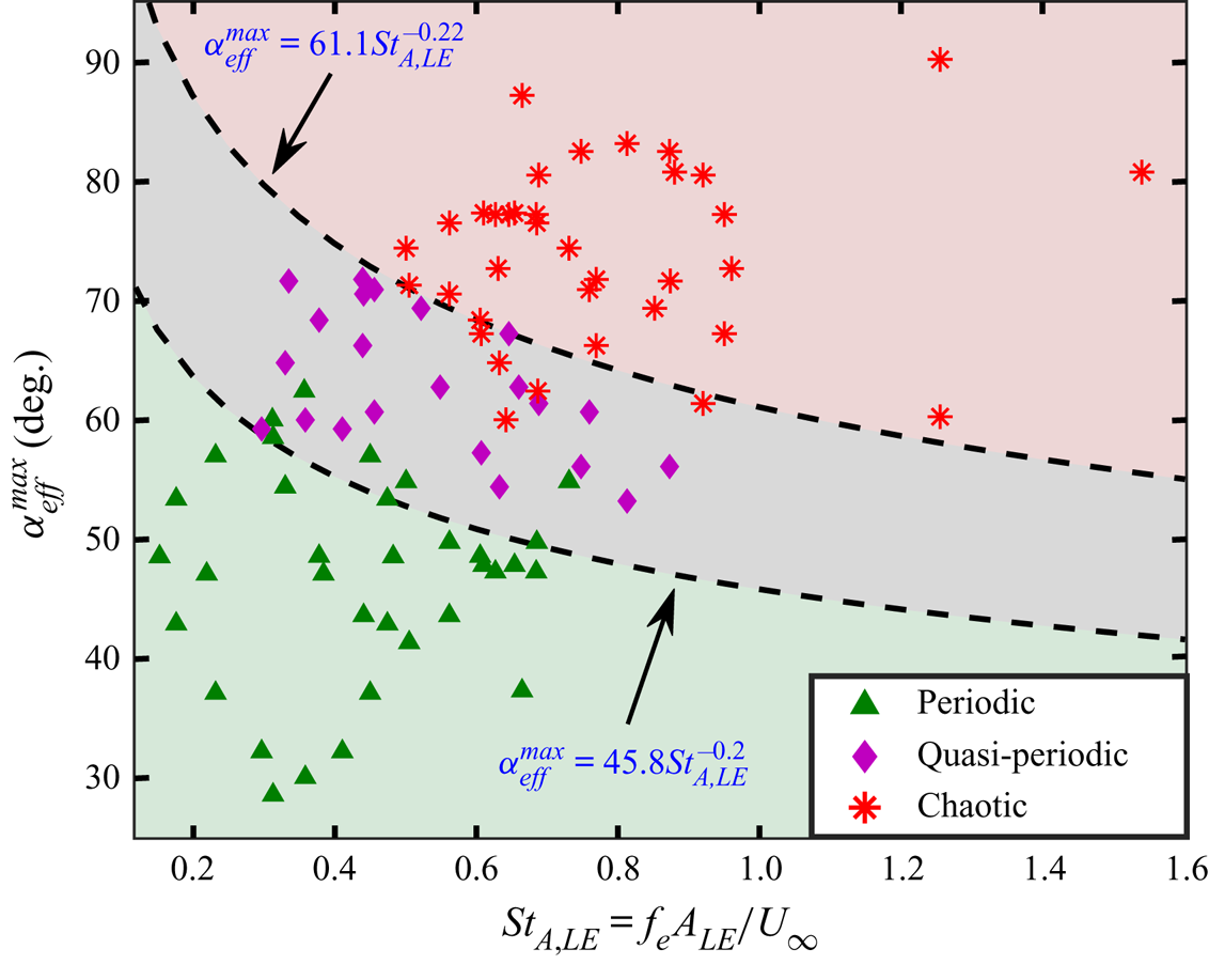
Figure 21. An order-to-chaos map ( $\alpha _{eff}^{max}$ versus $St_{A,LE}$) exhibiting the three distinct regions corresponding to qualitatively different dynamical states.
Dynamical transition from periodicity to robust chaos happens via local or global bifurcation routes through one or more intermediate dynamical states. The transition regime corresponds to those dynamical states for different kinematic conditions. The success of the present classification approach lies in pinpointing the periodic and robust chaotic regions with reasonable accuracy. Fundamentally, a portion of the periodic regime may still remain ‘entangled’ with a portion of the transition regime, and similarly a portion of the chaotic regime with that of the transition regime. However, it is definitely possible to identify distinct regions of periodicity and chaos, and an in-between ‘entangled’ regime of transition dynamics. The transition regime is identified as a collection of all possible transitional states. The exact dynamics for the entire transition regime may not be known a priori from this classification, and one would need a case-by-case investigation to comment on that. Note that the current model to define the order-to-chaos boundaries is a first step based on the present simulations, and the main focus was to identify a reduced-order parametric space by combining the effects of the most relevant kinematic quantities and developing generalised transition boundaries in that reduced space.
In summary, a total of 100 different parametric cases were simulated in this study. Among the  $36$ periodic points, $30$ were classified correctly, and among the $40$ chaotic cases, $35$ were classified correctly by the proposed transition boundaries in figure 21. This gives an accuracy of more than $85\,\%$, which is quite encouraging, especially in the light of the severe limitations of the existing non-dimensional quantities. Here are the main contributions made: (i) effective non-dimensional parameters were identified to track the qualitative changes in the flow field; (ii) a transition regime was identified where all transition states could be accommodated between order and chaos. Above this regime, robust chaos can be expected, and below, regular periodic dynamics.
5.2. Verification with the existing literature
In this subsection, the robustness of the proposed transition model is tested with existing data from the literature. This is demonstrated in figure 22 by calculating the  $\alpha _{eff}^{max}$ and $St_{A,LE}$ values for a series of data collected from the published results of different research groups reporting dynamical transition in flapping systems. The cases are as follows.
(i) Lewin & Haj-Hariri (Reference Lewin and Haj-Hariri2003): pure plunging elliptic-shaped foil with
$12\,\%$ thickness at $\kappa h = 0.8$, $1.0$, $1.2$ and $1.5$, with fixed $\kappa = 5.714$, $Re = 500$; plotted as $\blacksquare$.(ii) Deng et al. (Reference Deng, Sun, Teng, Pan and Shao2016): pure plunging NACA0015 aerofoil at
$A_D = 2.0$ and $Sr = 0.1$ to $0.55$ in steps of $0.05$, $Re = 1700$; plotted as $\blacktriangleright$.(iii) Badrinath et al. (Reference Badrinath, Bose and Sarkar2017): pure plunging NACA0012 aerofoil at
$h = 0.4$, $0.913$ and $1.2$, with fixed $\kappa = 2.0$, $Re = 1000$; plotted as $\blacktriangleleft$.(iv) Majumdar et al. (Reference Majumdar, Bose and Sarkar2020a,Reference Majumdar, Bose and Sarkarb): pure plunging elliptic-shaped foil with
$12\,\%$ thickness at $h = 0.25$, $0.375$, $0.4125$ and $0.475$, with fixed $\kappa = 4.0$, $Re = 300$; plotted as $\boldsymbol {+}$.(v) Zaman et al. (Reference Zaman, Young and Lai2017): pure pitching NACA0012 aerofoil at
$\theta _0 = 20^{\circ }$, $30^{\circ }$, $38^{\circ }$, $45^{\circ }$, $50^{\circ }$ and $58^{\circ }$, with fixed $\kappa = 8.0$, with the pitching axis being at the quarter-chord location, $Re = 500$; plotted as $\blacktriangledown$.(vi) Lentink et al. (Reference Lentink, Van Heijst, Muijres and Van Leeuwen2010): simultaneous pitching–heaving elliptic foil with
$5\,\%$ thickness at the dimensionless heave amplitude $A^{*} (= A/c) = 1.0$ and $2.0$ (where $A$ is the heave amplitude), $\alpha _0 = 15^{\circ }$, dimensionless heave length $\lambda ^{*} (= U_\infty /fc) = 3$ to $13$ in steps of $2$, $\phi = {\rm \pi}/2$, with the pitching axis being at the mid-chord location, $Re = 1000$; plotted as $\boldsymbol {\times }$.(vii) Bose & Sarkar (Reference Bose and Sarkar2018): simultaneous pitching–plunging NACA0012 aerofoil at
$h = 0.5$, $0.85$ and $1.25$, $\alpha = 15^{\circ }$, $\kappa = 2.0$, $\phi = {\rm \pi}/2$, with the pitching axis being at the quarter-chord location, $Re = 1000$; plotted as $\bullet$.


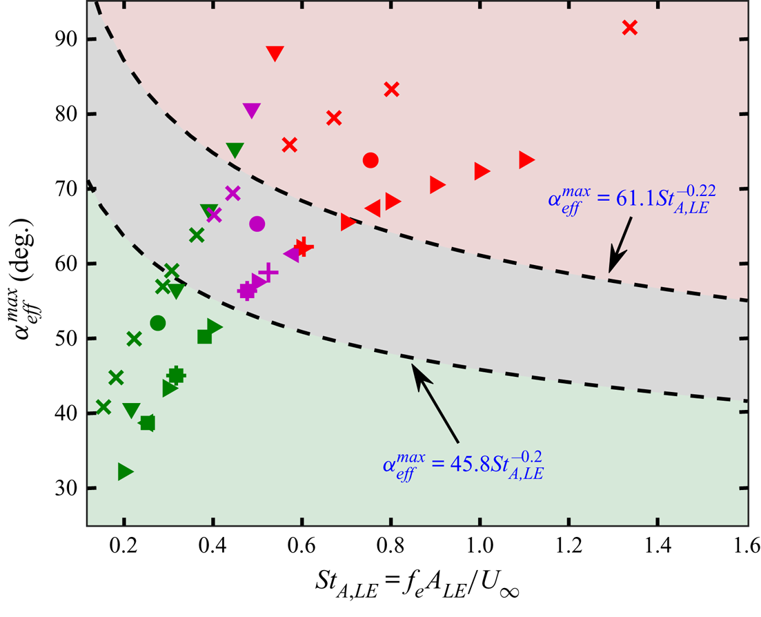
Figure 22. Validating the proposed transitional boundaries with the reporting of earlier works by different research groups. Markers are used as follows:  $\blacksquare$, Lewin & Haj-Hariri (Reference Lewin and Haj-Hariri2003); $\blacktriangleright$, Deng et al. (Reference Deng, Sun, Teng, Pan and Shao2016) (pure plunge); $\blacktriangleleft$, Badrinath et al. (Reference Badrinath, Bose and Sarkar2017); $\boldsymbol {+}$, Majumdar et al. (Reference Majumdar, Bose and Sarkar2020a,Reference Majumdar, Bose and Sarkarb); $\blacktriangledown$, Zaman et al. (Reference Zaman, Young and Lai2017); $\boldsymbol {\times }$, Lentink et al. (Reference Lentink, Van Heijst, Muijres and Van Leeuwen2010); and $\bullet$, Bose & Sarkar (Reference Bose and Sarkar2018). Colourcode: green if the dynamical state corresponding to the data point was reported to be periodic, red if it was reported to be chaos, and purple if the reported dynamical state exhibited transitionary signature in the respective literature.
The mathematical symbols used in the above description are as given in their respective articles. The markers in figure 22 are colour coded based on the dynamical states reported in the respective literature, i.e. green if the data point was reported as periodic, red if it was reported as chaotic, and purple if the data point was transitionary. As described in the previous paragraph, the cases taken from the literature involve various combinations of different kinematic parameters, flapping motions (pure plunge, pure pitch, simultaneous pitch–plunge), foil shapes and thicknesses, etc. Despite the variety of the parametric combinations, their dynamical states corroborate very well the proposed transitional boundaries, giving credibility to the present order-to-chaos map. A few exceptions have also been observed in the case of pure pitching at  $\theta _0 = 45^{\circ }$ and $50^{\circ }$ from Zaman et al. (Reference Zaman, Young and Lai2017). Among the 42 cases taken from the literature, 15 data points have been identified as periodic as per the present model, and all of them were also reported to be periodic in their respective studies. On the other hand, out of the 13 data points that fall above the shaded transition region as chaotic, only 11 were actually called chaotic in their respective studies. Thus out of 28 cases, 26 have been classified correctly, demonstrating an accuracy of around $93\,\%$. These results strengthen the efficacy of the proposed transition boundaries for demarcating the periodic and chaotic parametric sets in terms of $\alpha _{eff}^{max}$ and $St_{A,LE}$.
6. Conclusions
Effects of a wide variety of kinematic conditions on the dynamical transition in the wake of a flapping foil have been investigated by simulating a large number of parametric combinations (a total of 100 different cases) using an IBM-based in-house Navier–Stokes solver. It has been established already in the literature that the plunge amplitude and flapping frequency are two essential parameters that can dictate the dynamical nature of the flow field. This study reveals that other parameters, such as pitch amplitude ( $\theta _0$), pitching axis location ( $x_0$), foil thickness, type of kinematics, and phase offset ( $\phi$) between pitch and plunge motions, can also play very important roles in influencing the wake dynamics. The present study has also established that the chaotic transition in the flow field is strongly correlated with the strength of the primary LEV. Beyond a certain strength, the growth and separation of the LEV structure become chaotic, which eventually gets propagated to the trailing wake through LEV–TEV interactions in the subsequent cycles.
One of the main contributions of the present study is the introduction of two new non-dimensional quantities ( $St_{A,LE}$ and $\alpha _{eff}^{max}$) to capture the physical effect of the parametric variations considered in the study. The proposed dimensionless parameters can capture the important effects of the speed and the angle with which the foil interacts with the inflow. Changes in key parametric quantities reflect directly on the $\alpha _{eff}^{max}$– $St_{A,LE}$ pair, which is not true for the conventionally used non-dimensional numbers defined in the literature for specific kinematic situations. The other important contribution of the study is to propose generalised transition boundaries and an order-to-chaos map in terms of the newly proposed non-dimensional parameters. Published data from the existing literature have also been utilised to confirm the proposed boundaries. Despite the wide variety of parametric combinations, the dynamical states from both new and published data corroborate very well the proposed transitional boundaries, giving credibility to the order-to-chaos map.
Supplementary material
Supplementary materials are available at https://doi.org/10.1017/jfm.2022.385.
Declaration of interest
The authors report no conflict of interest.
Appendix A
The derivation of  $\alpha _{eff}$ is given here. For any point on the chord line located at a distance $s$ from the leading edge, its position along the $y$-direction can be written as
 \begin{equation} y_s = y_p - (s-x_0)\sin\theta.\end{equation}
Note that the pitch motion is clockwise positive, and plunge is positive along the positive  $y$-axis. The velocity at the $s$ location can be obtained from the time derivation of (A1) as
 \begin{equation} \dot{y}_s = \dot{y}_p - (s-x_0)\dot{\theta}\cos\theta. \end{equation}
Hence the average downwash velocity induced by the entire chord can be estimated as
 \begin{equation} W ={-}\frac{\displaystyle\int_{0}^{c}\dot{y}_s \, {{\rm d}}s}{\displaystyle\int_{0}^{c} \, {{\rm d}}s} ={-}\frac{1}{c} \int_{0}^{c} \{ \dot{y}_p - (s-x_0)\dot{\theta} \cos\theta \} \, {{\rm d}}s ={-}\left[\dot{y}_p - \left(\frac{c}{2} - x_0 \right) \dot{\theta} \cos\theta \right].\end{equation}
Finally, the effective AoA is given by
 \begin{equation} \alpha_{eff} = \theta - \tan^{{-}1} \left[\frac{W}{U_{\infty}}\right] = \theta - \tan^{{-}1} \left[\frac{1}{U_{\infty}} \left\{ \dot{y}_p - \left(\frac{c}{2} - x_0 \right) \dot{\theta} \cos\theta \right\} \right].\end{equation}
Appendix B
Figure 23(a) presents a plot in terms of non-dimensional parameters  $\kappa h$ versus $\kappa$ for all the parametric cases discussed in § 3.3.1. All those parametric cases collapse on just four data points ( $\kappa h = 1.0, 1.5, 1.9,2.5$). Evidently, the different dynamical states that belong to these parametric combinations ( $\phi$ variation) cannot be distinguished through these non-dimensional parameters. Similarly, non-dimensional parameters $A_D$ and $St_D$ (proposed by Godoy-Diana et al. Reference Godoy-Diana, Marais, Aider and Wesfreid2009) are also not suitable. The $A_D$ versus $St_D$ plot for the same cases is shown in figure 23(b). Here, the data points get mixed up and no pattern can be identified for the different dynamical states involved. As in these parametric cases $f_e$, $D$ and $U_{\infty }$ were not changed, a constant $St_D = 0.0764$ appears for all the cases, and the $A_D$ value hovers within the range $2.01 < A_D < 12.57$. Note that for a given $\kappa h$, a $\phi$ pair that is symmetric about the zero mean line (such as $\phi = {\rm \pi}/4 \ \& \ 7{\rm \pi} /4$ or $\phi = {\rm \pi}/2 \ \& \ 3{\rm \pi} /2$) result in the same $A_D$, even though the pair may exhibit very different dynamics. As was shown in figure 8, $\phi = {\rm \pi}/2$ and $\phi = 3{\rm \pi} /2$ at $\kappa h = 0.375$ manifest different dynamics (periodic and chaotic, respectively), though both have the same $A_D$ value of $6.62$. A $\tau _D$ versus $1/St_D$ plot has also been made here in figure 23(c), as proposed by Lagopoulos et al. (Reference Lagopoulos, Weymouth and Ganapathisubramani2019). No clear demarcation between the different dynamical states can be found here either. Thus in the light of the above discussion, the limitations of the earlier approaches in demarcating different dynamical regimes encountered presently are evident.
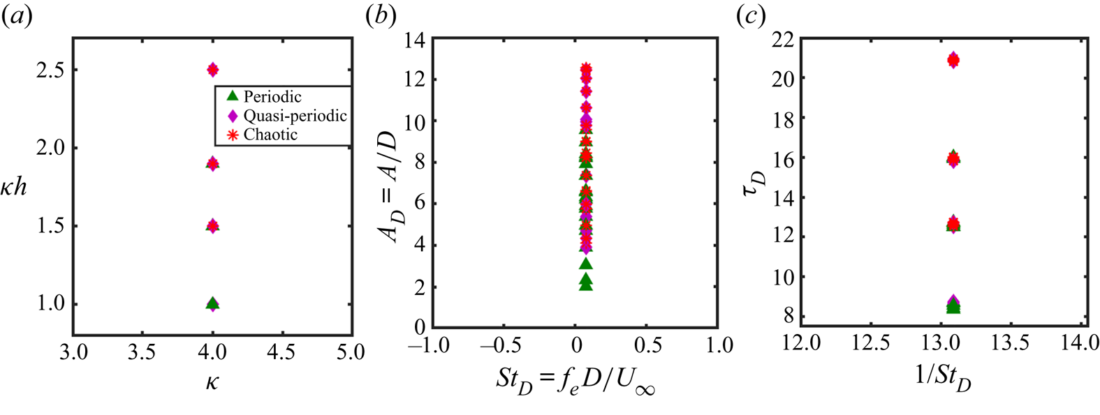
Figure 23. The parametric cases of § 3.3.1 presented in terms of the conventional non-dimensional numbers used by different research groups.
Appendix C
The effect of pivot location on the dynamical states of the flow field is small at  $\phi = {\rm \pi}/2$ and $3{\rm \pi} /2$, but it is quite tangible for $\phi = {\rm \pi}$ and $2{\rm \pi}$. In order to understand the different trends at different $\phi$, one needs to look into the respective $(St_{A,LE}, \alpha _{eff}^{max})$ pair values. This is because these quantities capture the two critical aspects – the leading-edge speed and the relative orientation with which the foil interacts with the incoming flow – that are the fundamental factors that affect the LEV formation and growth, and in turn, dictate the dynamical characteristics of the flow field. Figure 24 shows the $(St_{A,LE}, \alpha _{eff}^{max})$ pairs corresponding to the 12 parametric cases obtained by varying $\phi$ and $x_0$ (as presented in § 3.3.3). The cases corresponding to $x_0 = 0.25$, $0.5$ and $0.75$ are plotted using the markers $\boldsymbol {+}$, $\blacksquare$ and $\bullet$, respectively. The markers are colour coded as green, purple or red if they appear to be periodic, quasi-periodic or chaotic from the flow simulations, respectively.
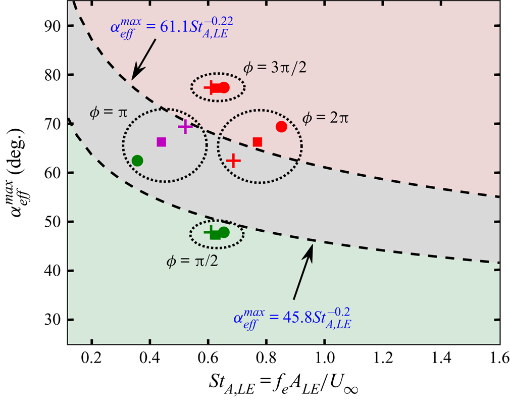
Figure 24. Variation in  $(St_{A,LE}, \alpha _{eff}^{max})$ pairs as the pivot location and phase offset are varied. Cases corresponding to $x_0 = 0.25$, $0.5$ and $0.75$ are plotted using the markers $\boldsymbol {+}$, $\blacksquare$ and $\bullet$, respectively. The markers are colour coded as green, purple or red if they appear to be periodic, quasi-periodic or chaotic from the flow simulations, respectively.
Note that in figure 24, the three data points at  $\phi = {\rm \pi}/2$ are seen to be sufficiently inside the periodic regime and are close to each other. This implies that these three cases correspond to sufficiently low leading-edge speed and effective AoA, and are thus associated with a stable periodic LEV behaviour. This results in periodic flow fields. At $\phi = 3{\rm \pi} /2$, the three data points corresponding to three different $x_0$ values are sufficiently inside the chaotic regime and are close to each other (figure 24). These cases correspond to substantially high leading-edge speed and effective AoA, and as a result are associated with chaotic LEV growth resulting ultimately in chaotic flow fields. Hence the dynamics at $\phi = {\rm \pi}/2$ and $\phi = 3{\rm \pi} /2$ look largely independent of the pivot location.
The cases of  $\phi = {\rm \pi}$ and $\phi = 2{\rm \pi}$ fall in the transition regime. At $\phi = {\rm \pi}$, as the pivot point is moved from the quarter-chord to the three-quarter-chord location, both $St_{A,LE}$ and $\alpha _{eff}^{max}$ gradually decrease, and the data points move towards the periodic regime; see figure 24. This is because the flapping motion at this $\phi$ is such that the leading edge traverses comparatively smaller distance with a lower leading-edge speed, and takes lower effective AoA values as the pivot point moves towards the trailing edge. As a result, gradually more stable primary LEV structures are formed with increasing $x_0$, and therefore the flow field turns from quasi-periodic to periodic. At $\phi = 2{\rm \pi}$, $St_{A,LE}$ and $\alpha _{eff}^{max}$ increase, and the data points move towards the chaotic regime with an increase in $x_0$ (figure 24). At this $\phi$, the leading edge traverses higher distances with increased leading-edge speed, and the foil takes comparatively higher effective AoA values as $x_0$ increases. This leads to irregular formation of the primary leading-edge vortices having higher strength and more agility, which eventually make the overall flow field more irregular, as observed in § 3.3.3. In conclusion, movement of the pivot location from the leading edge towards the trailing edge affects the leading-edge flapping speed and the foil's relative orientation with respect to the incoming flow conversely for $\phi = {\rm \pi}$ and $2{\rm \pi}$. Hence the flow field behaves contrastingly at these two $\phi$ values. It gets regularised at $\phi = {\rm \pi}$, but becomes more and more irregular at $\phi = 2{\rm \pi}$ with increasing $x_0$. This explains the underlying reason behind the opposite trends of the dynamical states at $\phi = {\rm \pi}$ and $2{\rm \pi}$ observed in § 3.3.3.


 Open access

