


1 Introduction
Low-head hydropower plants such as tidal power or run-of-river plants are a promising contribution to meeting the world’s rising electrical power demand, provided the technology becomes economically profitable (Rourke, Boyle & Reynolds Reference Rourke, Boyle and Reynolds2010). A reliable physical model for an energy-converting system capturing the relevant physical effects is necessary for investment decisions and optimal installation and operation. Adcock, Draper & Nishino (Reference Adcock, Draper and Nishino2015) pointed out that the maximal extractable power from tidal energy is of major interest and an adequate modelling is therefore a crucial step.
1.1 Turbine array and representative turbine
For power extraction, hydrokinetic turbines are used as machines arranged in a fence, row or array (figure 1). We investigate a turbine placed in an array that is either extended to infinity in the lateral direction or spans the entire channel width. In this case, the separating streamlines between the turbines are straight and hence lines of symmetry (figure 1). This allows us to focus on a single turbine with bypass within a generic control volume as marked in figure 1.

Figure 1. Top view of a turbine array. The flow is from left to right. Thin solid lines are streamlines and thick solid lines are turbine discs. It is assumed that the turbines are positioned sufficiently distant in the flow direction so that the upstream flow is uniform at the position labelled as [1]. Provided that the array spans the complete channel, the streamlines between two turbines are straight and it is sufficient to consider one representative turbine only. The sectional view A–A of a representative turbine is shown in figure 5.
The flow is considered as quasi-stationary. For run-of-river plants, this is obviously valid. For tidal power, the channel flow is quasi-stationary for a cycle time  $T\approx 4.5\times 10^{4}~\text{s}\gg l/\sqrt{gh_{0}}$. With the length of the tidal channel $l\sim 10{-}100~\text{km}$ and the undisturbed water depth in the channel $h_{0}\sim 10{-}100~\text{m}$ the mentioned condition is usually fulfilled. Only for very long, $l\sim 100~\text{km}$, and at the same time very shallow, $h_{0}\sim 10~\text{m}$, channels do transient effects become relevant.
With the assumptions of (i) straight separating streamlines and (ii) quasi-stationary flow, the presented model is in accordance with the asymptotic theories of Garrett & Cummins (Reference Garrett and Cummins2007), Whelan et al. (Reference Whelan, Thomson, Graham and Peiro2007), Whelan, Graham & Peiro (Reference Whelan, Graham and Peiro2009), Houlsby, Draper & Oldflield (Reference Houlsby, Draper and Oldflield2008) and Polagye (Reference Polagye2009) analysing a generic turbine in quasi-stationary flow. As will be shown, the cited existing theories for power extraction are only asymptotically valid for small blockage  $\unicode[STIX]{x1D70E}\rightarrow 0$ or small turbine power, i.e. low turbine head $H_{T}\rightarrow 0$. Note that $Fr_{0}\rightarrow 0$ implies $H_{T}\rightarrow 0$.
The aim of this paper is to generalise the asymptotic validity of the mentioned theories to the complete range of blockage ratio, turbine head and Froude number. Based on the presented and experimentally validated axiomatic theory, the upper limit for tidal power with lateral bypass is derived (cf. figures 18 and 19).
Secondary effects like centred and staggered arrangements and partially blocked tidal channels as discussed, for example, by Vennell (Reference Vennell2012), Draper & Nishino (Reference Draper and Nishino2014), Nishino & Willden (Reference Nishino and Willden2013), Gupta & Young (Reference Gupta and Young2017) and Bonar et al. (Reference Bonar, Chen, Schnabl, Venugopal, Borthwick and Adcock2019) are not in the scope of this paper.
1.2 Quasi-stationary models of power extraction from an open-channel flow
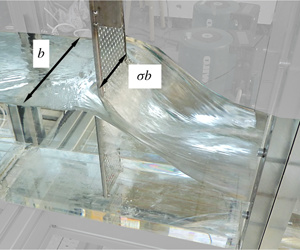
The turbines of the array may be axial-flow or cross-flow machines operating with ducts or diffusers (Roberts et al. Reference Roberts, Thomas, Sewell, Khan, Balmain and Gillman2016). The axis of rotation may be horizontal or vertical. The water depth in typical applications is about 1.5 to 3 times as deep as the turbine diameter of axial machines (Stallard et al. Reference Stallard, Collings, Feng and Whelan2013). For vertical-axis cross-flow machines like Darrieus rotors, the turbine may even penetrate the free water surface, causing a deformation of the free surface due to gravity similar to the observation of Leonardo da Vinci in the 16th century (da Vinci Reference da Vinci1510) (figure 2a).

Figure 2. (a) Sketch made by Leonardo da Vinci in the 16th century (da Vinci Reference da Vinci1510). A plate placed in the flow causes a drag force and thus a change in the water depth and convective momentum transport. (b) Water head drop caused by a momentum and energy sink due to a partial blockage at the open-channel test rig (see § 3). The turbine is represented by a perforated plate. There is no turbine volume flow,  $Q_{T}\equiv 0$, in (a), whereas $Q_{T}>0$ in our experiment (b).
All turbines have in common that they act as a momentum and energy sink to the flow. This sink is distributed over the turbines’ cross-section  $A_{T}$. In addition, energy is dissipated due to mixing in the wake of the turbine. For practical and ecological reasons $A_{T}$ is smaller than the channel cross-section $A_{1}=bh_{1}$, with the channel width $b$ and the upstream water depth $h_{1}$ (cf. figures 2b and 5). Garrett & Cummins (Reference Garrett and Cummins2007), Whelan et al. (Reference Whelan, Thomson, Graham and Peiro2007, Reference Whelan, Graham and Peiro2009), Houlsby et al. (Reference Houlsby, Draper and Oldflield2008) and Polagye (Reference Polagye2009) define the blockage as $\unicode[STIX]{x1D70E}:=A_{T}/A_{1}$.
Garrett & Cummins (Reference Garrett and Cummins2005) pointed out that the design and operation of a turbine array will slow down an undisturbed flow velocity  $u_{0}$ (denoted by index 0) to the approaching velocity $u_{1}<u_{0}$, resulting in an increase of the water depth $h_{1}>h_{0}$ in the upstream flow. This effect can only be neglected if the turbine array disturbs the flow only marginally. Thus, $u_{0}$ and $h_{0}$ are in general not independent scales for the problem.
Recognising this, Pelz (Reference Pelz2011) introduced the effective head  $H_{\mathit{eff}}:=z_{1}-z_{2}+h_{0}+u_{0}^{2}/2g$ with the ground level $z$, water depth $h$, velocity $u$ and gravitational body force $g$. The effective head $H_{\mathit{eff}}$ is independent of design, operation and downstream flow conditions. Hence, it is the natural scale for the energy conversion in any open-channel flow. For the considered problem, the upstream ground level $z_{1}$ equals the downstream ground level $z_{2}$. Thus, in this case, the effective head $H_{\mathit{eff}}$ reduces to the specific energy $H_{\mathit{eff}}=E_{0}=h_{0}+u_{0}^{2}/2g$.
Pelz (Reference Pelz2011) derived an upper limit for the power extraction from an open-channel flow without bypass, i.e. for the special case  $\unicode[STIX]{x1D70E}=1$. Using the first law of thermodynamics, the upper limit for the power extracted by the turbine from the flow, $P_{T}/\unicode[STIX]{x1D702}_{T}<P_{\mathit{avail}}/2:=\unicode[STIX]{x1D71A}bg^{3/2}(2/5H_{\mathit{eff}})^{5/2}$, can be derived. Hence, the coefficient of performance is limited in any case to $C_{P}:=P_{T}/P_{\mathit{avail}}\leqslant C_{P,max}=\unicode[STIX]{x1D702}_{T}/2$, where $\unicode[STIX]{x1D702}_{T}$ is the turbine efficiency and $\unicode[STIX]{x1D71A}$ is the fluid density (the subscript $max$ denotes the maximum possible value of $C_{P}$ for any design, operation and boundary condition). Here $C_{P,max}=\unicode[STIX]{x1D702}_{T}/2$ is a constant reference value independent of the boundary conditions, as shown in figure 3.

Figure 3. Upper limit of the coefficient of performance  $C_{P,max}/\unicode[STIX]{x1D702}_{T}=(P_{T,max}/\unicode[STIX]{x1D702}_{T})/P_{\mathit{avail}}$ versus Froude number of the undisturbed flow, $Fr_{0}=u_{0}/\sqrt{gh_{0}}$, for $\unicode[STIX]{x1D70E}=1$. For free-surface flow, the available power $\unicode[STIX]{x1D71A}u_{0}^{3}A_{T}/2$ defined by Betz (Reference Betz1920) leads to an undesired increase of $C_{P,max}$ with decreasing Froude number of the undisturbed flow. Hence, the ‘Betz limit’ $16/27$ should only be used for the asymptotic limit $\unicode[STIX]{x1D70E}\rightarrow 0$, $\overline{H}_{T}\rightarrow 0$, $Fr_{0}\rightarrow 0$. The available power $2\unicode[STIX]{x1D71A}g^{3/2}b\,(2/5H_{\mathit{eff}})^{5/2}$ defined by Pelz (Reference Pelz2011) yields a constant upper limit for $\unicode[STIX]{x1D70E}=1$: $(C_{P}/\unicode[STIX]{x1D702}_{T})_{max}=1/2$. For $\unicode[STIX]{x1D70E}\leqslant 1$ the upper limit is given in figure 18, depending on the downstream water depth $\overline{h}_{2}:=h_{2}/H_{\mathit{eff}}$.
Betz (Reference Betz1920) modelled the complementary limiting case  $\unicode[STIX]{x1D70E}\rightarrow 0$. Only for $\unicode[STIX]{x1D70E}\rightarrow 0$ is the approaching velocity $u_{0}$ unaffected by the turbine design and operation, and $u_{0}$ may serve as an independent scale for the energy extraction. Consequently, Betz defined $P_{avail,\unicode[STIX]{x1D70E}\rightarrow 0}:=\unicode[STIX]{x1D71A}u_{0}^{3}A_{T}/2$ as the available power. For the asymptotic limit $\unicode[STIX]{x1D70E}\rightarrow 0$, $Fr_{0}\rightarrow 0$ the upper limit is the well-known ‘Betz limit’ $C_{P,max,\unicode[STIX]{x1D70E}\rightarrow 0}:=P_{T}/P_{avail,\unicode[STIX]{x1D70E}\rightarrow 0}\leqslant 16\,\unicode[STIX]{x1D702}_{T}/27$ (figure 3).
In the context of tidal power, it becomes more and more obvious that this limit is exceeded using the reference  $\unicode[STIX]{x1D71A}u_{0}^{3}A_{T}/2$ for ideal and non-ideal turbine fences and arrays (Garrett & Cummins Reference Garrett and Cummins2007; Vennell Reference Vennell2013). A simple analysis (appendix A) shows that the ‘Betz limit’ becomes infinity for $Fr_{0}\rightarrow 0$, $\unicode[STIX]{x1D70E}=1$: $C_{P,Betz}\rightarrow 2\unicode[STIX]{x1D702}_{T}(2/5)^{5/2}Fr_{0}^{-3}$ (figure 3).
Garrett & Cummins (Reference Garrett and Cummins2007) generalised the Betz case for  $0<\unicode[STIX]{x1D70E}\leqslant 1$ but ignored any gravitational influence on the free surface. This conflicts with the first law of thermodynamics as figure 10 of this paper shows: the model of Garrett & Cummins (Reference Garrett and Cummins2007) predicts a power extraction above the physically possible value of $\unicode[STIX]{x1D702}_{T}/2$. An enhanced ‘streamtube’ model was proposed by Whelan et al. (Reference Whelan, Thomson, Graham and Peiro2007, Reference Whelan, Graham and Peiro2009), Houlsby et al. (Reference Houlsby, Draper and Oldflield2008) and Polagye (Reference Polagye2009) taking into account the deformation of the free surface due to gravity. However, this model still ignores the deformation of the turbine streamtube and the change in flux of kinetic energy and momentum across the turbine. Thus, for high blockage $\unicode[STIX]{x1D70E}$, high turbine head $H_{T}$ and high downstream Froude number $Fr_{2}$, the respective model yields unphysical behaviour. A critical assessment shows that the proposed models of Houlsby et al. (Reference Houlsby, Draper and Oldflield2008) and Polagye (Reference Polagye2009) are in fact identical to the one proposed by Whelan et al. (Reference Whelan, Thomson, Graham and Peiro2007, Reference Whelan, Graham and Peiro2009).

Figure 4. Different approaches to modelling the influence of the free surface on the turbine streamtube of a hydrokinetic turbine placed in an open-channel flow: (I) constant water head and neglected influence on turbine streamtube (Garrett & Cummins Reference Garrett and Cummins2007); (II) change in water head and neglected influence on turbine streamtube (Whelan et al. Reference Whelan, Thomson, Graham and Peiro2007, Reference Whelan, Graham and Peiro2009; Houlsby et al. Reference Houlsby, Draper and Oldflield2008; Polagye Reference Polagye2009); and (III) turbine streamtube deformation considered (this paper).
Figure 4 sketches the three different modelling approaches. Known theories I and II adapt the approach of Betz (Reference Betz1920) or Glauert (Reference Glauert1926) to hydrokinetic turbines in a free-surface flow.
In models I and II the inflow into the turbine, section  $[+]$, is considered to be immediately in front of the turbine of cross-section $A_{T}$. The outflow, section $[-]$, is considered to be immediately behind the turbine. Hence, the authors implicitly assumed the flow to be in a local equilibrium just upstream and downstream of the turbine. However, this implicit assumption is only valid for the asymptotic case of small blockage and turbine power, i.e. $\unicode[STIX]{x1D70E}\rightarrow 0$ and turbine head $\overline{H}_{T}\rightarrow 0$.
For relevant blockage, Froude number and turbine head, the asymptotic simplifications  $A_{+}\approx A_{-}\approx A_{T}$ and $u_{+}\approx u_{-}$ made in models I and II are not admissible. The flow field near the free surface differs from the one near the ground, and thus the gradients immediately behind the turbine are too large and the distribution of pressure and velocity is unknown. In this case, stream filament theory is not applicable (Spurk Reference Spurk1997). This is the reason why section $[-]$ has to be further downstream where the gradients are small. As a result $A_{+}\neq A_{-}\neq A_{T}$. Consequently, the flux terms in front, $A_{+}u_{+}^{n}$, and behind, $A_{-}u_{-}^{n}$, the turbine are only equal for $n=1$ (mass flux) but not for $n=2,3$: the change of momentum and kinetic energy flux across the disc is relevant for the turbine model itself but was ignored so far.
As this paper indicates, the asymptotic approximation  $A_{+}=A_{-}=A_{T}$ for $\unicode[STIX]{x1D70E}\rightarrow 0$, $Fr_{2}\rightarrow 0$, $H_{T}\rightarrow 0$, as done by Garrett & Cummins (Reference Garrett and Cummins2007), Whelan et al. (Reference Whelan, Thomson, Graham and Peiro2007, Reference Whelan, Graham and Peiro2009), Houlsby et al. (Reference Houlsby, Draper and Oldflield2008) and Polagye (Reference Polagye2009), leads to an overestimated energy extraction for non-asymptotic conditions conflicting with either the continuity or the energy equation (cf. figures 10–15). Experiments of Myers & Bahaj (Reference Myers and Bahaj2007), studies by means of computational fluid dynamics by Kolekar & Banerjee (Reference Kolekar and Banerjee2015) as well as the experiments shown in this paper (figure 2) reveal this limitation of existing theories.
To summarise, model I (Garrett & Cummins Reference Garrett and Cummins2007) ignores any interaction of the turbine array with the free surface. In model II (Whelan et al. Reference Whelan, Thomson, Graham and Peiro2007, Reference Whelan, Graham and Peiro2009; Houlsby et al. Reference Houlsby, Draper and Oldflield2008; Polagye Reference Polagye2009) the influence of the turbine on the free surface is considered, but the interaction of gravity with the turbine streamtube is ignored. Theories I and II are asymptotically justified for  $\unicode[STIX]{x1D70E}\rightarrow 0$, $H_{T}\rightarrow 0$. The general approach III takes the interaction of the turbine streamtube with the free surface into account and $A_{+}\!\neq \!A_{-}$ applies. The variables $A_{+}$, $A_{-}$, $u_{+}$ and $u_{-}$ become unknowns, requiring additional equations to close the problem.
For a truly axiomatic approach and in order to derive an upper limit for the power extraction, we consider a special case of III allowing only lateral bypass but no bypass ahead of and underneath the turbine (hereinafter referred to as model III) (cf. figures 2b and 5). This approach results in a closed system of equations including the additional unknowns  $h_{+}=A_{+}/\unicode[STIX]{x1D70E}b$, $h_{-}=A_{-}/\unicode[STIX]{x1D70E}b$, $u_{+}$ and $u_{-}$ (see § 2), without the need for further assumptions about the separation of the flow above and below the turbine. Thus, it is possible to derive a physically well-founded upper limit for any immersion depth of turbines of width $\unicode[STIX]{x1D70E}b$. It may be seen as a consistent generalisation of the limiting case $\unicode[STIX]{x1D70E}=1$, treated by Pelz (Reference Pelz2011). The generalised theory allows for a rigorous optimisation and hence the derivation of the desired upper limit shown in figure 18.
1.3 Independent variables and boundary conditions
As discussed, for  $\unicode[STIX]{x1D70E}\rightarrow 0$ the undisturbed velocity $u_{0}$ is the independent variable. However, for relevant power extraction from a tidal stream, this limiting case is unrealistic as Garrett & Cummins (Reference Garrett and Cummins2005) pointed out. They showed that for an optimal control of the power extraction from a tidal channel $Q_{1,opt}=Q_{0}/\sqrt{3}$ must hold. This may be reached by an optimally controlled operation considering the downstream flow condition $Fr_{2}$ or the downstream water depth $\overline{h}_{2}:=h_{2}/H_{\mathit{eff}}$ for a given design parameter $\unicode[STIX]{x1D70E}$ and $u_{1}\neq u_{0}$. For a tidal channel the downstream water surface does not change when entering the downstream basin due to Newton’s third law ‘actio est reactio’: the streamlines are parallel, and thus there is no pressure change normal to the streamlines and the water depth of two parallel streamtubes is equal. Hence, $\overline{h}_{2}$ is in fact a boundary condition to the flow (see the analogy to gas dynamics in appendix B). In conclusion we have a parameter for (i) design, (ii) operation and (iii) boundary condition. (i) The design of a generic turbine field is sufficiently described by the blockage ratio $\unicode[STIX]{x1D70E}$. (ii) The turbine operator controls the head drop across the turbine $H_{T}/\unicode[STIX]{x1D702}_{T}:=P_{T}/(\unicode[STIX]{x1D702}_{T}\unicode[STIX]{x1D71A}gQ_{T})$. (iii) The boundary condition is given either by $\overline{h}_{2}$ or by $Fr_{2}$.
In previous research often  $Fr_{1}$ and $h_{1}$ were chosen as boundary conditions. Since the flow variables depend on each other, it is possible to transform the boundary conditions. From $\overline{C}_{P}(\unicode[STIX]{x1D70E},\overline{H}_{T},\overline{Fr}_{2})$ and $Fr_{1}(\unicode[STIX]{x1D70E},\overline{H}_{T},Fr_{2})$ it is possible to derive $\overline{C}_{P}(\unicode[STIX]{x1D70E},\overline{H}_{T},Fr_{1})$. Nevertheless, the choice of $Fr_{1}$ or $h_{1}$ as boundary condition is not practical when looking for the optimal power coefficient $C_{P,opt}$, since both $Fr_{1}$ and $h_{1}$ depend on the design, i.e. blockage $\unicode[STIX]{x1D70E}$, and the operation, i.e. turbine head $\overline{H}_{T}$. (Note that for the asymptotic limit $\unicode[STIX]{x1D70E}\rightarrow 0$, $Fr_{0}\rightarrow 0$ the often used induction factor $a:=u_{\ast }/u_{1}$ and the turbine head $\overline{H}_{T}$ are equivalent determining the operation of the turbine. But in general, $\unicode[STIX]{x1D70E}>0$, the turbine head $\overline{H}_{T}$ is appropriate indicating the operating point, being common in the context of fluids engineering, turbomachinery and open-channel flow.)
The power extraction per unit width depends on
 $$\begin{eqnarray}\frac{P_{T}}{\unicode[STIX]{x1D702}_{T}b}=f(g,\unicode[STIX]{x1D71A},H_{\mathit{eff}},\unicode[STIX]{x1D70E},H_{T}/\unicode[STIX]{x1D702}_{T},h_{2}).\end{eqnarray}$$
A dimensional analysis yields
 $$\begin{eqnarray}\overline{C}_{P}:=\frac{C_{P}}{\unicode[STIX]{x1D702}_{T}}:=\frac{P_{T}/\unicode[STIX]{x1D702}_{T}}{P_{\mathit{avail}}}=\overline{C}_{P}(\unicode[STIX]{x1D70E},\overline{H}_{T},\overline{h}_{2})\leqslant 1/2,\end{eqnarray}$$
 with  $\overline{H}_{T}:=H_{T}/(H_{\mathit{eff}}\unicode[STIX]{x1D702}_{T})$ and the available power for the general case
 $$\begin{eqnarray}P_{\mathit{avail}}:=2\unicode[STIX]{x1D71A}bg^{3/2}\left({\textstyle \frac{2}{5}}H_{\mathit{eff}}\right)^{5/2}.\end{eqnarray}$$
 The factor  $(2/5)^{5/2}$ originates of course not from the dimensional analysis but from the energy balance. The factor $2$ originates from the assumed ‘ideal’ machine (Pelz Reference Pelz2011).
Similarly, the volumetric efficiency  $\unicode[STIX]{x1D702}_{V}:=Q_{T}/Q_{1}$ with turbine volume flow $Q_{T}$ and total volume flow $Q_{1}<Q_{0}$ is also a function of (i) design parameter $\unicode[STIX]{x1D70E}$, (ii) operation parameter $\overline{H}_{T}$ and (iii) downstream condition $\overline{h}_{2}$ or $Fr_{2}$:
 $$\begin{eqnarray}\unicode[STIX]{x1D702}_{V}:=\frac{Q_{T}}{Q_{1}}=\unicode[STIX]{x1D702}_{V}(\unicode[STIX]{x1D70E},\overline{H}_{T},\overline{h}_{2})\leqslant 1.\end{eqnarray}$$
 Since  $\unicode[STIX]{x1D702}_{V}<1$ for $\unicode[STIX]{x1D70E}<1$, the mixing of the turbine volume flow $Q_{T}=\unicode[STIX]{x1D702}_{V}Q_{1}$ and the bypass volume flow $(1-\unicode[STIX]{x1D702}_{V})Q_{1}$ causes the dissipated power $P_{D,mix}$ in the mixing zone between [ $\ast$] and [ $2$] (see figure 5). The dimensionless mixing loss $\unicode[STIX]{x1D700}$ is a function of the same independent variables:
 $$\begin{eqnarray}\unicode[STIX]{x1D700}:=\frac{P_{D,mix}}{\unicode[STIX]{x1D71A}\,g\,Q_{1}\,(H_{1}-H_{2})}=\unicode[STIX]{x1D700}(\unicode[STIX]{x1D70E},\overline{H}_{T},\overline{h}_{2})\leqslant 1.\end{eqnarray}$$
With these definitions, the downstream total head can be expressed as
 $$\begin{eqnarray}\frac{H_{2}}{H_{\mathit{eff}}}=1-\unicode[STIX]{x1D702}_{V}\frac{\overline{H}_{T}}{1-\unicode[STIX]{x1D700}}\end{eqnarray}$$
and the total efficiency as
 $$\begin{eqnarray}\unicode[STIX]{x1D702}:=\frac{P_{T}}{P_{T}+P_{D,mix}+P_{D,T}}=\unicode[STIX]{x1D702}_{T}(1-\unicode[STIX]{x1D700}).\end{eqnarray}$$
 On a system level it is necessary to determine all three measures:  $\overline{C}_{P}$ to benchmark the overall energetic quality of the system, $\unicode[STIX]{x1D702}_{V}$ to gain a valuable measure for the turbine design and $\unicode[STIX]{x1D700}$ to benchmark the dissipation loss influenceable by the system designer. To optimise the power extraction of a cascade or array of turbines, i.e. turbines aligned in a row in flow direction, $C_{P}$ and $\unicode[STIX]{x1D700}$ have to be known.
The aim of this study is threefold. Firstly, comparing  $\overline{C}_{P},\unicode[STIX]{x1D702}_{V},\unicode[STIX]{x1D700}=f(\unicode[STIX]{x1D70E},\overline{H}_{T},Fr_{2})$ or $f(\unicode[STIX]{x1D70E},\overline{H}_{T},\overline{h}_{2})$ of the presented model with the asymptotically valid theories of Garrett & Cummins (Reference Garrett and Cummins2007), Whelan et al. (Reference Whelan, Thomson, Graham and Peiro2007, Reference Whelan, Graham and Peiro2009), Houlsby et al. (Reference Houlsby, Draper and Oldflield2008) and Polagye (Reference Polagye2009). Here, it is revealed that these models are limited to the asymptotic limit $\unicode[STIX]{x1D70E}\rightarrow 0$ or $Fr_{2}\rightarrow 0$ or $\overline{H}_{T}\rightarrow 0$. Secondly, discussing the function $\overline{C}_{P}(\unicode[STIX]{x1D70E},\overline{H}_{T},\overline{h}_{2})$ including the parameter range resulting in a downstream surge wave. This can only be achieved by treating the free surface of the problem in a physically appropriate way. Thirdly, discussing the upper limit $C_{P,opt}(\unicode[STIX]{x1D70E},\overline{h}_{2})$ for the power extraction as a function of blockage and downstream flow condition:
 $$\begin{eqnarray}\overline{C}_{P,opt}(\unicode[STIX]{x1D70E},\overline{h}_{2})=\max _{\overline{H}_{T}}C_{P}(\unicode[STIX]{x1D70E},\overline{H}_{T},\overline{h}_{2})\end{eqnarray}$$
 (the subscript  $opt$ denotes optimal values for given design parameter $\unicode[STIX]{x1D70E}$ and boundary condition $\overline{h}_{2}$).
The paper is structured as follows. Model III is derived in § 2. The experimental apparatus is described in § 3.1, while we validate our model in § 3.2 with the help of an assessable integral measure, the drag force and water depth  $h_{\ast }$. We discuss the system behaviour and compare the mentioned models in § 4.1. The transient behaviour for sub- and supercritical flow is analysed in § 4.2. Finally, the optimisation problem (1.8) is treated and discussed in § 4.3. The conclusion of this work is given in § 5.
2 Generic model of a hydrokinetic turbine with lateral bypass
The turbine is modelled, for both the analysis and the experiment, as a planar momentum and energy sink of constant width  $\unicode[STIX]{x1D70E}b$ placed vertically in a stationary flow, ranging from the bottom of the channel to above the free surface (figure 5). The origin of the $z$ coordinate is placed at the channel bottom, for which zero slope is assumed, i.e. $z=0$. Therefore the total head $H$ is identical to the specific energy $E$.
$E$.

Figure 5. Momentum and energy sink with lateral bypass in an open channel as investigated in this paper. All solid lines are streamlines. Index 1 indicates disturbed approaching flow. Indexes  $+$ and $-$ are respectively in close proximity upstream and downstream of the turbine where the changes in flow direction are small. Index $\ast$ marks the position where the bypass and the turbine flow depths are again balanced due to ‘actio est reactio’ while index 2 is the position far downstream of the turbine.
The distribution of the flow quantities does not need to be known over each arbitrary cross-section of the streamtube; this is only necessary at the inlet and outlet of a streamtube representing one part of the model. In the presented model, we assume that the flow at the inlet and the outlet does not change significantly in the flow direction. For a free-surface flow, this assumes that the water depth  $h$ is only a slowly varying function of the coordinate in the flow direction $x$. In terms of dimensionless measures, the slope of the free surface shall be much smaller than one: $|h^{\prime }|=|\text{d}h/\text{d}x|\ll 1$. This is clearly not the case when modelling conditions directly downstream of a turbine, where a drag force $D$ in the free-surface flow is caused: immediately downstream of the turbine $h^{\prime }$ is negative and the absolute value may reach values of the order one (figure 2). Only at a distance downstream of the turbine is the asymptote $h^{\prime }\rightarrow 0$ reached, and thus the flow is sufficiently uniform and the pressure is given by a hydrostatic pressure distribution. This fact has to be considered in the momentum equation of the turbine streamtube, see (2.13) and (2.14), and was ignored in previous research. It results in $A_{+}>A_{-}$ and in a change in the momentum and energy flux through the turbine.
The energy extraction takes place between [ $+$] and [ $-$], i.e. the beneficial part $P_{T}:=\unicode[STIX]{x1D71A}gQ_{T}H_{T}$ and the dissipation within the turbine $P_{D,T}:=\unicode[STIX]{x1D71A}g\,Q_{T}h_{D,T}$ ( $h_{D,T}$ is the associated height loss) cause the turbine drag force $D$. This makes it accessible to a force measurement for the experimental model validation discussed in § 3.2. The bypass flow and the turbine flow show different flow depths due to streamline curvature. At one position downstream of the turbine, marked by an asterisk [ $\ast$] (figures 2, 5 and 6), the streamlines are straight and parallel. Hence, for dynamic reasons, Newton’s third law ‘actio est reactio’, the bypass and turbine flow show the same flow depth $h_{\ast }$, even though their velocities differ. The bypass and turbine flow mix from cross-section [ $\ast$] to [2], which is associated with considerable dissipation $P_{D,mix}:=\unicode[STIX]{x1D71A}g\,Q_{1}h_{D,mix}$. With this picture in mind, the generic control volume is considered to be composed of five control volumes (i)–(v) as sketched in figure 6. Each control volume is a streamtube:
(i) upstream turbine streamtube stretching from section [1] to section $[+]$,
(ii) turbine wake streamtube stretching from section
$[-]$ to section $[\ast ]$,(iii) turbine itself, with inlet section
$[+]$ and outlet section $[-]$,(iv) bypass streamtube stretching from section
$[1]$ to section $[\ast ]$, and(v) mixing (or wake) streamtube stretching from section
$[\ast ]$ to section [2].


Figure 6. Top view of the generic control volume being composed of control volumes (i)–(v).
Hence, there are five linear independent continuity equations – one for each streamtube – connecting 14 flow variables: three dimensionless lengths  $\unicode[STIX]{x1D702}_{V}$, $\unicode[STIX]{x1D6FD}_{\ast }$ and $\unicode[STIX]{x1D70E}$ measured in multiples of the channel width $b$, five dimensionless water depths $\overline{h}_{1}$, $\overline{h}_{+}$, $\overline{h}_{-}$, $\overline{h}_{\ast }$ and $\overline{h}_{2}$ related to the upstream energy height $H_{1}=H_{0}=E_{0}$ and six Froude numbers, i.e. dimensionless velocities, $Fr_{1}$, $Fr_{+}$, $Fr_{-}$, $Fr_{b}$, $Fr_{i}$ and $Fr_{2}$.
The flow through the turbine is described by three continuity equations starting with the continuity equation for the control volume (i) upstream of the turbine
 $$\begin{eqnarray}\unicode[STIX]{x1D702}_{V}Fr_{1}\overline{h}_{1}^{3/2}=\unicode[STIX]{x1D70E}Fr_{+}\overline{h}_{+}^{3/2},\end{eqnarray}$$
for control volume (iii) around the turbine
 $$\begin{eqnarray}Fr_{+}\overline{h}_{+}^{3/2}=Fr_{-}\overline{h}_{-}^{3/2}\end{eqnarray}$$
and for control volume (ii) downstream of the turbine
 $$\begin{eqnarray}\unicode[STIX]{x1D70E}Fr_{-}\overline{h}_{-}^{3/2}=\unicode[STIX]{x1D6FD}_{\ast }Fr_{i}\overline{h}_{\ast }^{3/2}.\end{eqnarray}$$
 This reveals that the volumetric efficiency  $\unicode[STIX]{x1D702}_{V}$ corresponds to the dimensionless width of the turbine streamtube at point [1]. The mass conservation for the bypass flow yields
 $$\begin{eqnarray}(1-\unicode[STIX]{x1D702}_{V})Fr_{1}\overline{h}_{1}^{3/2}=(1-\unicode[STIX]{x1D6FD}_{\ast })Fr_{b}\overline{h}_{\ast }^{3/2}\end{eqnarray}$$
and for the mixing zone
 $$\begin{eqnarray}[(1-\unicode[STIX]{x1D6FD}_{\ast })Fr_{b}+\unicode[STIX]{x1D6FD}_{\ast }Fr_{i}]\overline{h}_{\ast }^{3/2}=Fr_{2}\overline{h}_{2}^{3/2}.\end{eqnarray}$$
 Applying the energy equation to each streamtube yields five more equations considering the two energy sinks  $P_{T}/\unicode[STIX]{x1D702}_{T}$ and $P_{D,mix}$. For the power extraction, the energy equation for control volume (iii), expressed in terms of energy head, leads to
 $$\begin{eqnarray}\overline{h}_{+}\left(1+{\textstyle \frac{1}{2}}Fr_{+}^{2}\right)-\overline{h}_{-}\left(1+{\textstyle \frac{1}{2}}Fr_{-}^{2}\right)=\overline{H}_{T}.\end{eqnarray}$$
 Only in the asymptotic approximation for small blockage  $\unicode[STIX]{x1D70E}\rightarrow 0$ and low turbine head $\overline{H}_{T}\rightarrow 0$ (Garrett & Cummins Reference Garrett and Cummins2007; Whelan et al. Reference Whelan, Thomson, Graham and Peiro2007, Reference Whelan, Graham and Peiro2009; Houlsby et al. Reference Houlsby, Draper and Oldflield2008; Polagye Reference Polagye2009) does the difference in the flux of kinetic energy cancel out. For the relevant range of turbine power and blockage the flux terms must be taken into account.
For the mixing zone described by control volume (v), the energy equation yields
 $$\begin{eqnarray}\unicode[STIX]{x1D6FD}_{\ast }\frac{\overline{q}_{i}}{\overline{q}_{2}}\overline{h}_{\ast }\left(1+\frac{1}{2}Fr_{i}^{2}\right)+(1-\unicode[STIX]{x1D6FD}_{\ast })\frac{\overline{q}_{b}}{\overline{q}_{2}}\overline{h}_{\ast }\left(1+\frac{1}{2}Fr_{b}^{2}\right)-\overline{h}_{2}\left(1+\frac{1}{2}Fr_{2}^{2}\right)=\overline{h}_{D,mix},\end{eqnarray}$$
 with  $\overline{h}_{D,mix}:=h_{D,mix}/H_{\mathit{eff}}$. The values $\overline{q}_{i}=Fr_{i}\overline{h}_{\ast }^{3/2}$, $\overline{q}_{b}=Fr_{b}\overline{h}_{\ast }^{3/2}$ and $\overline{q}_{2}=Fr_{2}\overline{h}_{2}^{3/2}$ are the dimensionless specific volume flow rates at positions $[i]$, $[o]$ and [2], respectively. For the remaining control volumes, energy conservation yields
 $$\begin{eqnarray}\overline{h}_{1}\left(1+{\textstyle \frac{1}{2}}Fr_{1}^{2}\right)=\overline{h}_{+}\left(1+{\textstyle \frac{1}{2}}Fr_{+}^{2}\right)\end{eqnarray}$$
for the upstream part of the turbine flow (control volume (i)) and
 $$\begin{eqnarray}\overline{h}_{-}\left(1+{\textstyle \frac{1}{2}}Fr_{-}^{2}\right)=\overline{h}_{\ast }\left(1+{\textstyle \frac{1}{2}}Fr_{i}^{2}\right)\end{eqnarray}$$
for the downstream part of the turbine flow (control volume (ii)). For the bypass flow (iv), the energy equation is written
 $$\begin{eqnarray}\overline{h}_{1}\left(1+{\textstyle \frac{1}{2}}Fr_{1}^{2}\right)=\overline{h}_{\ast }\left(1+{\textstyle \frac{1}{2}}Fr_{b}^{2}\right).\end{eqnarray}$$
 The bypass flow is an accelerated flow for which the dissipation is usually small (Spurk Reference Spurk1997). Hence, dissipation is only considered for the decelerated flow starting from [ $\ast$].
A sixth energy equation is obtained by the definition of the upstream boundary condition
 $$\begin{eqnarray}\overline{H}_{1}=1=\overline{h}_{1}(1+Fr_{1}^{2}/2).\end{eqnarray}$$
The system of equations is completed by momentum equations formulated for the three rectangular streamtubes, since for curved, i.e. non-rectangular, streamtubes the pressure distribution along the axial coordinate is necessary but unknown. Firstly, the momentum balance for the mixing streamtube (v) reads
 $$\begin{eqnarray}\unicode[STIX]{x1D6FD}_{\ast }\overline{h}_{\ast }^{2}\left({\textstyle \frac{1}{2}}+Fr_{i}^{2}\right)+(1-\unicode[STIX]{x1D6FD}_{\ast })\overline{h}_{\ast }^{2}\left({\textstyle \frac{1}{2}}+Fr_{b}^{2}\right)=\overline{h}_{2}^{2}\left({\textstyle \frac{1}{2}}+Fr_{2}^{2}\right).\end{eqnarray}$$
 Secondly, the momentum equation for the turbine streamtube (iii) from [ $+$] to [ $-$] leads to
 $$\begin{eqnarray}\unicode[STIX]{x1D70E}\overline{h}_{+}^{2}\left({\textstyle \frac{1}{2}}+Fr_{+}^{2}\right)-\unicode[STIX]{x1D70E}\overline{h}_{-}^{2}\left({\textstyle \frac{1}{2}}+Fr_{-}^{2}\right)=\overline{D},\end{eqnarray}$$
 considering the dimensionless drag force  $\overline{D}:=D/\unicode[STIX]{x1D71A}gbH_{\mathit{eff}}^{2}$. As in the energy equation (2.6), the asymptotic approximation for small blockage and low turbine head (Garrett & Cummins Reference Garrett and Cummins2007; Whelan et al. Reference Whelan, Thomson, Graham and Peiro2007, Reference Whelan, Graham and Peiro2009; Houlsby et al. Reference Houlsby, Draper and Oldflield2008; Polagye Reference Polagye2009) does not show the difference in the flux terms. In general, the difference in momentum flux is relevant and therefore is taken into account in this paper. For the considered generic case, equations (2.6) and (2.13) are exact. This allows us to derive an axiomatically determined upper limit for tidal power with lateral bypass.
Thirdly and finally, we give the momentum equation for the generic control volume itself, i.e. the streamtube stretching from [1] to [2]:
 $$\begin{eqnarray}\overline{h}_{1}^{2}\left({\textstyle \frac{1}{2}}+Fr_{1}^{2}\right)-\overline{h}_{2}^{2}\left({\textstyle \frac{1}{2}}+Fr_{2}^{2}\right)=\overline{D}.\end{eqnarray}$$
 Thus, a system of 14 equations is obtained for the 14 variables  $\unicode[STIX]{x1D702}_{V}$, $\unicode[STIX]{x1D6FD}_{\ast }$, $h_{1}$, $Fr_{1}$, $h_{+}$, $Fr_{+}$, $h_{-}$, $Fr_{-}$, $h_{\ast }$, $Fr_{b}$, $Fr_{i}$, $h_{2}$, $\overline{h}_{D,mix}$ and $\overline{D}$. The system of equations is completed by three independent variables: the design parameter $\unicode[STIX]{x1D70E}$, the operational parameter $\overline{H}_{T}$ and the downstream boundary condition $Fr_{2}$. Alternatively to $Fr_{2}$, the downstream water depth $\overline{h}_{2}$ may be used as boundary condition. The upstream boundary condition $\overline{H}_{1}=1$ is always satisfied.
At the end of this section it is worth summarising the assumptions made and the resulting axiomatic character of the theory. Firstly, the flow is considered to be quasi-stationary and the separating streamlines between the turbines are straight. Secondly, the dissipation due to frictional forces is considered to take place within the turbine and mixing zone only and uniform velocity profiles are assumed at the inlet and outlet cross-sections. Thirdly, the turbine extends from the channel bottom to the surface.
The first two assumptions do not represent a strong limitation of the given theory and are explicitly or implicitly made by Garrett & Cummins (Reference Garrett and Cummins2007), Whelan et al. (Reference Whelan, Thomson, Graham and Peiro2007, Reference Whelan, Graham and Peiro2009), Houlsby et al. (Reference Houlsby, Draper and Oldflield2008) and Polagye (Reference Polagye2009) as well. The third assumption, the special topology, allows us to give an exact general valid theory and an exact upper limit for the power output. This is because the flux terms in the momentum and energy equation for the turbine are indeed relevant.
3 Experimental validation
So far there has been a lack of experimental validation of models I, II and III apart from the experiments done by Whelan et al. (Reference Whelan, Graham and Peiro2009). Thus, an open-channel test rig was designed. The set-up is presented in § 3.1. The experimental validation is given in § 3.2. The apparatus allows the observation of transient phenomena like surge waves, which are discussed in § 4.2 and shown in a movie (Metzler & Pelz Reference Metzler and Pelz2015), also available as a supplementary movie available at https://doi.org/10.1017/jfm.2020.99.
3.1 Experimental set-up

Figure 7. Open-channel test rig for measurements with defined values for the blockage ratio  $\unicode[STIX]{x1D70E}$, turbine head $\overline{H}_{T}$ and downstream Froude number $Fr_{2}$.
The Froude-scaled channel is designed with  $0.05\leqslant Fr_{0}\leqslant 1.4$ including the representative range for rivers and tidal currents. This experimental set-up serves to validate the derived model. The channel has a width of $b=0.20~\text{m}$, a height of 0.40 m and a length longer than 2.0 m. Figure 7 shows a photograph and a sketch of the test rig. From left to right the flow wells up and passes a flow straightener, which separates the plunge chamber from the inlet nozzle by means of two perforated plates. The inlet nozzle allows the flow $Q_{1}$ to stream smoothly into the entry of the measurement section. Most of the test rig is made of acrylic glass, which allows smooth surfaces and optical accessibility. The flow rate is measured by an in-line magnetic-inductive sensor. The photograph shows the three-dimensional traverse for the pitot tube used to measure the flow velocity profiles and the water levels, as an electrical circuit closes when the pitot tube comes in contact with the water.
In accordance with the introduced generic control volume, the turbine is modelled as an energy and momentum sink. A perforated plate extending from the bottom of the channel to above the free surface causes a drag force  $D$ (momentum sink) and the associated dissipation $P_{T}/\unicode[STIX]{x1D702}_{T}$ (energy sink) (figure 2b). By changing the plate width, four different blockage ratios $\unicode[STIX]{x1D70E}=\{0.25,0.5,0.75,1.0\}$ are realised. The turbine operation point $\overline{H}_{T}=\overline{H}_{T}(Q_{T})$ is varied using different plate perforations. The perforation is quantified by the plate’s porosity $\unicode[STIX]{x1D719}:=A_{void}/A_{T}$ with the perforated area $A_{void}$ of the plate and the total area $A_{T}$. The perforated plate is supported by a short beam, connected in the middle of the upper plate edge. This beam is designed as a strain gauge beam sensor to measure the drag force $D$. At the outlet [2], the flow is conditioned by an adjustable flow resistor, controlling the outlet Froude number $Fr_{2}$. All measurements discussed in this paper are taken at zero slope $\unicode[STIX]{x0394}z=0$ and stationary operation.
A pump is installed below the open channel to overcome the pressure losses within the closed loop, obtaining a Reynolds number of  $Re:=4u_{0}h_{0}/[(1+2\,h_{0}/b)\,\unicode[STIX]{x1D708}]>5\times 10^{4}$ with the kinematic viscosity of water $\unicode[STIX]{x1D708}=10^{-6}~\text{m}^{2}~\text{s}^{-1}$, undisturbed flow $u_{0}\geqslant 0.1~\text{m}~\text{s}^{-1}$ and water depth $h_{0}\leqslant 0.4~\text{m}$. Hence, the flow is well within the turbulent regime and the boundary layers are thin enough so that the velocity profiles can be approximated as block profiles at all inlet and outlet cross-sections of the five streamtubes. For the operation point $\unicode[STIX]{x1D70E}=0.5$, $Fr_{2}=0.5$ and $\unicode[STIX]{x1D719}=0.37$, example velocity profiles are shown in figure 8. The measurement grids consist of more than 250 points by one vertical cross-section and one measurement point is averaged over 3 s. The assumption of block velocity profiles is very well satisfied for the inlet and outlet sections [1] and [2]. At the estimated measurement section [ $\ast$] for the bypass flow [ $o$] and the inner flow [ $i$], the velocity distribution coefficients for energy and momentum flux (Chow Reference Chow1959), i.e. analysing the degree of homogeneity, are always lower than 1.5 and 1.2. Hence, for simplicity it is justified to set these coefficients to 1.0.

Figure 8. Isoclines of the measured axial velocity  $u=\text{const.}$ in $\text{m}~\text{s}^{-1}$ at cross-sections [1], $[\ast ]$ and [2] for the operation point $Fr_{2}=0.5$, $\unicode[STIX]{x1D70E}=0.5$ and $\unicode[STIX]{x1D719}=0.37$. The shown $\unicode[STIX]{x1D6FD}_{\ast }$ and $H_{2}$ are derived by solving the system of equations discussed in § 2.
3.2 Model validation
The energetic and kinematic measures  $C_{P}$, $\unicode[STIX]{x1D702}_{V}$ and $\unicode[STIX]{x1D700}$ are of major interest. However, for the chosen generic set-up, it is not possible to measure them explicitly and thus validate them. The determination of $C_{P}$, for example, requires either the measurement of $P_{T}$ and a known characteristic diagram of the turbine efficiency $\unicode[STIX]{x1D702}_{T}$ or the volume flow through the turbine $Q_{T}$ and the turbine head $H_{T}$. In the apparatus the energy is not extracted by the perforated plate but rather dissipated. Hence, $P_{T}$, $Q_{T}$ and $H_{T}$ are not directly accessible even thought present in the model set-up. However, the drag force $D$ and the water depth $h_{\ast }$ are in fact accessible integral variables and can be measured directly. As both quantities arise explicitly in two and six equations, respectively, they are implicitly linked to the other quantities (see § 2). To validate the system of equations, a semi-analytical simulation is performed.
The values of the measured variables, except the one used for validation, are set as boundary conditions in the semi-empirical simulation, i.e.  $Q_{1},h_{1},h_{\ast },h_{2},\unicode[STIX]{x1D70E}$ for the validation via drag force $D$ (figure 9a,c,e) and $Q_{1},h_{1},h_{2},D,\unicode[STIX]{x1D70E}$ for the validation via the water depth $h_{\ast }$ (figure 9b,d,f). The latter corresponds to the choice of independent variables for § 4 as discussed in § 1.3 due to $H_{1}=H_{1}(Q_{1},h_{1})$, $Fr_{2}=Fr_{2}(Q_{1},h_{2})$ and $H_{T}\propto D$. The remaining variables, including the left-out measured variable $D$ or $h_{\ast }$ respectively, are the unknowns of the system of equations and are estimated.
The system of equations is solved in MATLAB using the fmincon algorithm. The residual of the solution is below  $10^{-6}$, which guarantees that neither the measured variables nor the equations contradict each other and all equations are accurately solved. This chosen approach is known as a nonlinear observer model in control theory.
In order to take into account the influence of the uncertainty in the observed values on the predicted values, the semi-empirical simulation is integrated into a Monte Carlo simulation. In this process, the simulation is repeatedly solved (2000 iterations) with different values for the measured variables, normally distributed within their uncertainty range. From this follows a set of solutions, providing an uncertainty range for the estimation.
To validate the prediction quality of the different models, the observed drag force  $D$ is compared with the predicted drag force $D(Q_{1},h_{1},h_{\ast },h_{2},\unicode[STIX]{x1D70E})$ of each simulation (figure 9a,c,e). Similarly, figure 9(b,d,f) shows the observed depth $h_{\ast }$ over the predicted depths $h_{\ast }(Q_{1},h_{1},h_{2},D,\unicode[STIX]{x1D70E})$.

Figure 9. For each model: observed drag force  $D$ versus predicted drag force (a,c,e) and observed water depth $h_{\ast }$ versus predicted water depth (b,d,f) for various values of blockage ratios $\unicode[STIX]{x1D70E}=\{0.25,0.5,0.75\}$, downstream Froude numbers $Fr_{2}=\{0.2,0.3,0.4,0.5\}$ (marker size rising with Froude number) and plate porosity $\unicode[STIX]{x1D719}=\{0.26,0.37,0.48\}$. The solid line indicates the data trend, whereas the dotted bisecting line represents ideal results. The error bars represent the 95 % confidence interval.
It becomes evident that model I (Garrett & Cummins Reference Garrett and Cummins2007) overpredicts the drag force for high  $\unicode[STIX]{x1D70E}$ and $Fr_{2}$ (figure 9a). This can be explained as follows: the pressure downstream of the turbine is given as boundary condition. As the change in potential energy due to the water head drop is neglected by model I, an equivalent drag that produces the same downstream pressure by just decelerating the streamtube flow is predicted. This drag is obviously higher than with consideration of the water head drop. As approaches II (Whelan et al. Reference Whelan, Thomson, Graham and Peiro2007, Reference Whelan, Graham and Peiro2009; Houlsby et al. Reference Houlsby, Draper and Oldflield2008; Polagye Reference Polagye2009) and III (this paper) consider the water head drop above the turbine and thus a change in potential energy, the predicted forces are in good agreement with the measurement. Comparing measured and predicted water depth $h_{\ast }$ at position $[\ast ]$ downstream of the turbine, it can be seen that the predictions of Garrett & Cummins (Reference Garrett and Cummins2007) are obviously always higher than the measured depths due to the neglected water head drop, i.e. $h_{\ast ,I}=h_{1}$. Approaches II and III again show far better accordance. For high blockage and downstream Froude number, however, neglecting the influence on turbine streamtube (II) leads to a slight underprediction of $h_{\ast }$, i.e. an overprediction of the beneficial energy extraction over the mixing losses (see § 4.1).
It is worthwhile noting, even though not shown, that experiments performed with fully submerged perforated plates covering the whole width of the channel but allowing bypass flow above and underneath showed similar results.

Figure 10. Coefficient of performance versus turbine head  $\overline{H}_{T}$ for various values of blockage ratio $\unicode[STIX]{x1D70E}$ and downstream Froude number $Fr_{2}$. Solid lines represent the results of model III, presented in this paper. Dashed lines represent model II of Whelan et al. (Reference Whelan, Thomson, Graham and Peiro2007, Reference Whelan, Graham and Peiro2009), Houlsby et al. (Reference Houlsby, Draper and Oldflield2008) and Polagye (Reference Polagye2009) and dotted lines represent model I of Garrett & Cummins (Reference Garrett and Cummins2007). The optimum point of operation is marked by a small black circle, the conflict with the energy equation of model I by a triangle and the upper limit for $Fr_{2}=1$ by a large circle.
4 Results and discussion
In this section we first discuss the system behaviour for typical Froude numbers  $Fr_{2}\leqslant 0.5$ and compare the predictions of model III presented in this paper with models according to approaches I (Garrett & Cummins Reference Garrett and Cummins2007) and II (Whelan et al. Reference Whelan, Thomson, Graham and Peiro2007, Reference Whelan, Graham and Peiro2009; Houlsby et al. Reference Houlsby, Draper and Oldflield2008; Polagye Reference Polagye2009). Afterwards, the influence of the downstream Froude number is analysed up to supercritical flow of $Fr_{2}=2.0$ for a fixed turbine head $\overline{H}_{T}$ showing transient flow phenomena between sub- and supercritical downstream flow. Concluding, we discuss the optimal operational strategy $\overline{H}_{T,opt}$ for hydrokinetic turbines for given blockage $\unicode[STIX]{x1D70E}$ and downstream condition $\overline{h}_{2}$, yielding the optimal coefficient of performance $\overline{C}_{P,opt}$.
4.1 System behaviour and comparison with asymptotically valid models
To provide a benchmark for the planning and dimensioning of low-head hydropower plants, the energetic and kinematic measures that are relevant for system design are analysed. These measures are the coefficient of performance  $\overline{C}_{P}$, the normalised volumetric efficiency $\overline{\unicode[STIX]{x1D702}}_{V}:=\unicode[STIX]{x1D702}_{V}/\unicode[STIX]{x1D70E}$ and the mixing loss $\unicode[STIX]{x1D700}$. The three measures are calculated in terms of the independent parameter triple $(\unicode[STIX]{x1D70E},\overline{H}_{T},Fr_{2})$. In this section we focus on the plausibility and comparison of the different models. The complete picture of model III is given in figures 18–21, in which the optimal operational strategy and the upper limit are discussed (§ 4.3).
Each measure is plotted for four blockage ratios  $\unicode[STIX]{x1D70E}=\{0.25,0.5,0.75,1.0\}$ and two downstream Froude numbers $Fr_{2}=\{0.2,0.4\}$ versus the relative turbine head $\overline{H}_{T}$. Bold solid lines show the axiomatic result of model III presented in this paper. Thin solid lines represent model II of Whelan et al. (Reference Whelan, Thomson, Graham and Peiro2007, Reference Whelan, Graham and Peiro2009), Houlsby et al. (Reference Houlsby, Draper and Oldflield2008) and Polagye (Reference Polagye2009) and dashed lines represent model I of Garrett & Cummins (Reference Garrett and Cummins2007).

Figure 11. Normalised volumetric efficiency  $\overline{\unicode[STIX]{x1D702}}_{V}$ versus turbine head $\overline{H}_{T}$ for different values of blockage ratio $\unicode[STIX]{x1D70E}$ and downstream Froude number $Fr_{2}$. Solid lines represent the results of model III, presented in this paper. Dashed lines represent model II of Whelan et al. (Reference Whelan, Thomson, Graham and Peiro2007, Reference Whelan, Graham and Peiro2009), Houlsby et al. (Reference Houlsby, Draper and Oldflield2008) and Polagye (Reference Polagye2009) and dotted lines represent model I of Garrett & Cummins (Reference Garrett and Cummins2007). The conflict with the continuity equation of model II is marked by a triangle.
Figure 10 shows the influence of the turbine head  $\overline{H}_{T}$ on the coefficient of performance $\overline{C}_{P}$ for different downstream Froude numbers $Fr_{2}=0.2$ and 0.4. There is an increase of $\overline{C}_{P}$ as well as of the optimal turbine head $\overline{H}_{T,opt}$ (marked by a circle) with increasing blockage $\unicode[STIX]{x1D70E}$ and downstream Froude number $Fr_{2}$. It can be seen that the predictions of the different models are similar for low turbine head $\overline{H}_{T}$ or blockage $\unicode[STIX]{x1D70E}$. A comparison of models I, II and III gives: for low $\unicode[STIX]{x1D70E}=0.25$ all models are equivalent up to $\overline{H}_{T}\approx 0.15$, whereas for $\unicode[STIX]{x1D70E}>0.75$ the models start to differ significantly above $\overline{H}_{T}\approx 0.05$. The differences occur less early and are less critical for lower Froude numbers until for $Fr_{2}\rightarrow 0$ again, all results are identical. For independent variables $\unicode[STIX]{x1D70E}$, $\overline{H}_{T}$, $Fr_{2}$ beyond that region, model II of Whelan et al. (Reference Whelan, Thomson, Graham and Peiro2007, Reference Whelan, Graham and Peiro2009), Houlsby et al. (Reference Houlsby, Draper and Oldflield2008) and Polagye (Reference Polagye2009) and especially model I of Garrett & Cummins (Reference Garrett and Cummins2007) overestimate the energy extraction. This is due to the fact that these models assume an unaffected turbine streamtube that can expand freely without interacting with the surface. The water head drop, however, prevents that expansion, which becomes significant for higher $\unicode[STIX]{x1D70E}$, $\overline{H}_{T}$, $Fr_{2}$. The model of Garrett & Cummins (Reference Garrett and Cummins2007) even exceeds the upper limit of $\overline{C}_{P,max}=1/2$, e.g for $\unicode[STIX]{x1D70E}=0.75$, $Fr_{2}=0.4$ for $\overline{H}_{T}>0.5$ (for higher $\unicode[STIX]{x1D70E}$ and $Fr_{2}$ even earlier), which is obviously wrong since it conflicts with the first law of thermodynamics.

Figure 12. Mixing loss  $\unicode[STIX]{x1D700}$ versus turbine head $\overline{H}_{T}$ for various values of blockage ratio $\unicode[STIX]{x1D70E}$ and downstream Froude number $Fr_{2}$. Solid lines represent the results of model III, presented in this paper. Dashed lines represent model II of Whelan et al. (Reference Whelan, Thomson, Graham and Peiro2007, Reference Whelan, Graham and Peiro2009), Houlsby et al. (Reference Houlsby, Draper and Oldflield2008) and Polagye (Reference Polagye2009) and dotted lines represent model I of Garrett & Cummins (Reference Garrett and Cummins2007). The conflict with the energy equation of model II is marked by a triangle.
The second measure to be analysed, the normalised volumetric efficiency  $\overline{\unicode[STIX]{x1D702}}_{V}:=\unicode[STIX]{x1D702}_{V}/\unicode[STIX]{x1D70E}$, is plotted in figure 11. It becomes apparent which fraction of the volume flow enters the turbine, $Q_{T}=\unicode[STIX]{x1D702}_{V}Q_{1}$, or bypasses the turbine, $(1-\unicode[STIX]{x1D702}_{V})Q_{1}$. For the limit $\overline{H}_{T}\rightarrow 0$, the flow is undisturbed, which yields $\overline{\unicode[STIX]{x1D702}}_{V}=1$, since the turbine streamtube is not affected. For full blockage $\unicode[STIX]{x1D70E}=1$, there is no bypass flow and $\overline{\unicode[STIX]{x1D702}}_{V}\equiv 1$ is true for all flow conditions. For $\unicode[STIX]{x1D70E}<1$, increasing $\overline{H}_{T}$ and decreasing $Fr_{2}$, the volumetric efficiency decreases as the turbine has a higher resistance and thus more flow bypasses the turbine. For a too high turbine head the whole volume flow bypasses the turbine, leading to $\unicode[STIX]{x1D702}_{V}\rightarrow 0$. Therefore the coefficient of performance $\overline{C}_{P}$ vanishes (cf. figures 10 and 16). As for the coefficient of performance, the predictions of all models are similar for small independent variables $\unicode[STIX]{x1D70E}$, $\overline{H}_{T}$, $Fr_{2}$. For larger blockage, especially with higher Froude number and turbine head, model I according to Garrett & Cummins (Reference Garrett and Cummins2007) and especially model II according to Whelan et al. (Reference Whelan, Thomson, Graham and Peiro2007, Reference Whelan, Graham and Peiro2009), Houlsby et al. (Reference Houlsby, Draper and Oldflield2008) and Polagye (Reference Polagye2009) overestimate the volumetric efficiency. For the latter model and a blockage of $\unicode[STIX]{x1D70E}=0.75$, the volumetric efficiency increases with increasing turbine head. This is implausible and not representing the flow. Values $\overline{\unicode[STIX]{x1D702}}_{V}>1$, predicted by model II of Houlsby et al. (Reference Houlsby, Draper and Oldflield2008), are wrong.
The mixing loss  $\unicode[STIX]{x1D700}$ is shown in figure 12. Comparing the four plots, it is evident that the mixing loss decreases with increasing blockage $\unicode[STIX]{x1D70E}$. For the limit $\unicode[STIX]{x1D70E}\rightarrow 1$ the loss vanishes as there is no bypass and thus no mixing. High turbine head and low Froude number, however, lead to inefficient wake mixing. Especially when considering turbine cascades, the turbine head $\overline{H}_{T}$ should be adjusted to minimise mixing losses. The predictions of model II show implausible decreasing mixing loss for high blockage $\unicode[STIX]{x1D70E}=0.75$.
To further study the influence of the blockage ratio,  $\overline{C}_{P}$, $\overline{\unicode[STIX]{x1D702}}_{V}$ and $\unicode[STIX]{x1D700}$ are plotted against $\unicode[STIX]{x1D70E}$ for four fixed relative turbine heads $\overline{H}_{T}=\{0.1,0.2,0.3,0.4\}$ and two downstream Froude numbers $Fr_{2}=\{0.2,0.4\}$.

Figure 13. Coefficient of performance versus blockage ratio  $\unicode[STIX]{x1D70E}$ for various values of turbine head $\overline{H}_{T}$ and downstream Froude number $Fr_{2}$. Solid lines represent the results of model III, presented in this paper. Dashed lines represent model II of Whelan et al. (Reference Whelan, Thomson, Graham and Peiro2007, Reference Whelan, Graham and Peiro2009), Houlsby et al. (Reference Houlsby, Draper and Oldflield2008) and Polagye (Reference Polagye2009) and dotted lines represent model I of Garrett & Cummins (Reference Garrett and Cummins2007). The optimum point of operation at $Fr_{2}=1$ is marked by a circle and the conflict with the energy equation of model I by a triangle.
Figure 13 shows the influence of the blockage ratio  $\unicode[STIX]{x1D70E}$ on the coefficient of performance $\overline{C}_{P}$. Obviously the power extraction is increasing with increasing blockage and is higher for higher Froude number. For a fixed Froude number $Fr_{2}$, a minimal blockage $\unicode[STIX]{x1D70E}_{min}$ is needed to create a head drop $\overline{H}_{T}>0$ so that there is no power extraction for low $\unicode[STIX]{x1D70E}<\unicode[STIX]{x1D70E}_{min}$. As already discussed earlier, the different models are similar for low ( $\unicode[STIX]{x1D70E},Fr_{2},\overline{H}_{T}$). In accordance with figure 10 similar results for a wide range of blockages are only given for turbine heads $\overline{H}_{T}\leqslant 0.1$. For higher turbine heads, results are only similar for quite low blockages or Froude number. Otherwise the coefficient of performance is overpredicted by models I and II. Model I is even exceeding the upper limit $\overline{C}_{P,max}=1/2$ as stated earlier.

Figure 14. Normalised volumetric efficiency  $\overline{\unicode[STIX]{x1D702}}_{V}$ versus turbine head $\overline{H}_{T}$ for different values of blockage ratio $\unicode[STIX]{x1D70E}$ and downstream Froude number $Fr_{2}$. Solid lines represent the results of model III, presented in this paper. Dashed lines represent model II of Whelan et al. (Reference Whelan, Thomson, Graham and Peiro2007, Reference Whelan, Graham and Peiro2009), Houlsby et al. (Reference Houlsby, Draper and Oldflield2008) and Polagye (Reference Polagye2009) and dotted lines represent model I of Garrett & Cummins (Reference Garrett and Cummins2007). The optimum point of operation at $Fr_{2}=1$ is marked by a circle and the conflict with the continuity equation of model II by a triangle.
The normalised volumetric efficiency  $\overline{\unicode[STIX]{x1D702}}_{V}$ is plotted in figure 11 against the blockage ratio $\unicode[STIX]{x1D70E}$. The volumetric efficiency is increasing with increasing Froude number and obviously increasing with the blockage ratio. For full blockage, $\unicode[STIX]{x1D70E}=1$, $\overline{\unicode[STIX]{x1D702}}_{V}$ has to be equal to one no matter the flow state. This is indeed true for models I and III, whereas the result of model II (Whelan et al. Reference Whelan, Thomson, Graham and Peiro2007, Reference Whelan, Graham and Peiro2009; Houlsby et al. Reference Houlsby, Draper and Oldflield2008; Polagye Reference Polagye2009) predicts $\overline{\unicode[STIX]{x1D702}}_{V}>1$, which is obviously wrong. A further analysis shows that in this case the turbine streamtube at position [ $\ast$] is supposed to cover more than the available channel cross-section $bh_{\ast }$. This is due to the head drop, and thus a reduction of the floated channel area, without considering the back-effect on the turbine streamtube, i.e. a reduction of the streamtube area.

Figure 15. Mixing loss  $\unicode[STIX]{x1D700}$ versus blockage ratio $\unicode[STIX]{x1D70E}$ for various values of turbine head $\overline{H}_{T}$ and downstream Froude number $Fr_{2}$. Solid lines represent the results of model III, presented in this paper. Dashed lines represent model II of Whelan et al. (Reference Whelan, Thomson, Graham and Peiro2007, Reference Whelan, Graham and Peiro2009), Houlsby et al. (Reference Houlsby, Draper and Oldflield2008) and Polagye (Reference Polagye2009) and dotted lines represent model I of Garrett & Cummins (Reference Garrett and Cummins2007). The optimum point of operation at $Fr_{2}=1$ is marked by a circle and the conflict with the energy equation of model II by a triangle.
As the volumetric efficiency  $\overline{\unicode[STIX]{x1D702}}_{V}$ is increasing, the mixing inefficiency $\unicode[STIX]{x1D700}$ is decreasing. Both values are qualitatively similar and roughly related by the approximation $\overline{\unicode[STIX]{x1D702}}_{V,opt}\approx 1-\unicode[STIX]{x1D700}_{opt}$ (cf. figures 14 and 15). For high blockages, $\unicode[STIX]{x1D70E}\rightarrow 1$, and no bypass flow, $\unicode[STIX]{x1D700}\rightarrow 0$, again only models I (Garrett & Cummins Reference Garrett and Cummins2007) and III (this paper) yield plausible results for the mixing zone.
Concluding, this section can be summarised as follows:
(i) Beneficial and non-beneficial power extraction is dependent on the independent parameters
$\unicode[STIX]{x1D70E}$, $\overline{H}_{T}$, $Fr_{2}$ or $\unicode[STIX]{x1D70E}$, $\overline{H}_{T}$, $\overline{h}_{2}$. The coefficient of performance $\overline{C}_{P}$ is monotonically increasing with $\unicode[STIX]{x1D70E}$ and $Fr_{2}<1$. For $\overline{H}_{T}$ there is an upper limit for the power extraction in the range $0.0<\overline{H}_{T,opt}(\unicode[STIX]{x1D70E},Fr_{2})<0.5$ (cf. figures 18 and 19). This maximum has to be taken into account by the operator. The upper limit is consistent with the findings of Pelz (Reference Pelz2011) and is addressed in more detail in § 4.3. In order to reduce mixing losses after the turbine, it is recommended to operate at high $\unicode[STIX]{x1D70E}$, high $Fr_{2}$ and low $\overline{H}_{T}$.(ii) For low blockages
$\unicode[STIX]{x1D70E}<0.25$ or for low turbine heads $\overline{H}_{T}<0.1$, the results of all models are similar as they are for low Froude numbers $Fr_{2}\rightarrow 0$. Thus, the water head drop and the turbine streamtube deformation are negligible for $\unicode[STIX]{x1D70E},\overline{H}_{T},Fr_{2}\rightarrow 0$.(iii) For higher energy-extraction the predictions of the models differ. With increasing
$\unicode[STIX]{x1D70E}$, $\overline{H}_{T}$ and $Fr_{2}$ the differences become more significant. For a blockage at the latest from $\unicode[STIX]{x1D70E}=0.75$, neglecting the turbine streamtube deformation even leads to implausible results for known models I and II (in terms of either $\overline{C}_{P}$ or $\overline{\unicode[STIX]{x1D702}}_{V}$ and $\unicode[STIX]{x1D700}$, respectively).


In conclusion, only within the limits  $\unicode[STIX]{x1D70E}<0.25$, $\overline{H}_{T}<0.1$ or $Fr_{2}\rightarrow 0$ may the previous models I and II serve as an approximation.
4.2 Transient flow phenomena
In order to achieve a profound understanding of the entire system, a wider Froude range  $0\leqslant Fr_{2}\leqslant 2$ including supercritical flow states is considered in the following. Figure 16 shows $\overline{C}_{P}$ versus the downstream Froude number $Fr_{2}$ for, as an example, turbine head $\overline{H}_{T}=\overline{H}_{T,max}=2/5$ for different blockage ratios $\unicode[STIX]{x1D70E}$.

Figure 16. Coefficient of performance  $\overline{C}_{P}(\unicode[STIX]{x1D70E},\overline{H}_{T}=2/5,Fr_{2})$ versus the downstream Froude number $Fr_{2}$ for various values of blockage ratio $\unicode[STIX]{x1D70E}$.

Figure 17. Blockage ratio  $\unicode[STIX]{x1D70E}$ versus the downstream Froude number $Fr_{2}$ depending on the turbine head showing the thresholds of the downstream Froude number $Fr_{2,lb}$ and $Fr_{2,ub}$.
One can draw three conclusions from this figure. Firstly, the coefficient of performance increases with increasing blockage ratio  $\unicode[STIX]{x1D70E}$. The bold solid line, $\unicode[STIX]{x1D70E}=1$, reaches the maximum $\overline{C}_{P,max}=1/2$ for $Fr_{2}=1$. Thus, the results presented here are a consistent generalisation of the results presented by Pelz (Reference Pelz2011) for different blockage ratios. Secondly, for subcritical downstream flow $Fr_{2}<1$, the coefficient of performance increases with increasing downstream Froude number until a threshold $Fr_{2,lb}$ is reached. At this threshold, the downstream flow becomes transient and a rarefaction wave occurs in the experiment (the term rarefaction wave is adopted from gas dynamics; see appendix B). This rarefaction wave starts behind the turbine, and moves downstream while the downstream flow becomes supercritical $Fr_{2}>1$. The vice versa case, an upstream-moving hydraulic jump, i.e. a surge wave, is shown in a movie (Metzler & Pelz Reference Metzler and Pelz2015). For $Fr_{2}>Fr_{2,ub}$, the flow becomes quasi-stationary again. As the simulation is based on a quasi-stationary system of equations, no meaningful solutions exist for $Fr_{2,lb}<Fr_{2}<Fr_{2,ub}$, i.e. the residuals are more than five orders of magnitude higher than for $Fr_{2}<Fr_{2,lb}$ and $Fr_{2}>Fr_{2,ub}$. Both thresholds $Fr_{2,lb}$ and $Fr_{2,ub}$ depend on the blockage ratio and turbine head. The transition is given by the dashed line in figure 16. Hence, by the transition from $Fr_{2,lb}$ to $Fr_{2,ub}$, the flow is transient and there is no solution of the quasi-stationary model. Thirdly, for still increasing downstream Froude number and supercritical flow, the coefficient of performance decreases. Hence, the coefficient of performance reaches its maximum close to the thresholds.
These thresholds are shown in figure 17 as well. This figure analyses the blockage ratio versus the downstream Froude number depending on the turbine head isolines. The dependency of the thresholds on the turbine head becomes visible and the region  $Fr_{2,lb}<Fr_{2}<Fr_{2,ub}$ becomes smaller for decreasing turbine head. Thus, the lower and upper thresholds reduce to one transition line at $Fr_{2}=1$ for $\overline{H}_{T}\rightarrow 0$. The area below the hatched line is physically impossible as the volumetric efficiency $\unicode[STIX]{x1D702}_{V}$ has to be positive.

Figure 18. Isolines of maximum possible coefficient of performance  $\overline{C}_{P,opt}$ for a given blockage and downstream water depth $\overline{h}_{2}$. Critical water depth $\overline{h}_{2,crit}=2/3$.
4.3 Optimal operation of a tidal turbine
As stated in § 1.3 and appendix B, the parameter triple  $(\unicode[STIX]{x1D70E},\overline{H}_{T},Fr_{2})$ can be equivalently replaced by $(\unicode[STIX]{x1D70E},\overline{H}_{T},\overline{h}_{2})$ as considered in the following. Since the downstream water depth $\overline{h}_{2}$ is given by the tidal system and the blockage ratio $\unicode[STIX]{x1D70E}$ by the system designer, the turbine head $\overline{H}_{T}$ is the only adjustable parameter of this parameter triple. Thus, the operator has to adjust the turbine head in order to achieve optimal operation. Here, optimal operation means reaching the maximum possible coefficient of performance $\overline{C}_{P,opt}$ for given parameters.
An optimal coefficient of performance  $\overline{C}_{P,opt}(\unicode[STIX]{x1D70E},\overline{h}_{2})$ could be achieved examining $\unicode[STIX]{x2202}\overline{C}_{P}/\unicode[STIX]{x2202}\overline{H}_{T}=0$. However, the coefficient of performance is not continuously differentiable due to the transition from $Fr_{2,lb}$ to $Fr_{2,ub}$ (see § 4.2). Hence, the optimal coefficient of performance is evaluated numerically.
The optimal coefficient of performance depending on the downstream water depth  $\overline{h}_{2}$ and the blockage ratio $\unicode[STIX]{x1D70E}$ is depicted in figure 18. The optimum operation point with $\overline{C}_{P,opt}=\overline{C}_{P,max}=1/2$ is reached for full blockage $\unicode[STIX]{x1D70E}=1$ and a critical water depth $\overline{h}_{2}=2/5$, which is consistent with the findings of Pelz (Reference Pelz2011) (see circular marker in figures 16 and 18). At a fixed blockage ratio $\unicode[STIX]{x1D70E}<1$ and for subcritical downstream flow $Fr_{2}<1$, the optimal coefficient of performance increases with decreasing downstream depth $\overline{h}_{2}$. Crossing the transition line, the downstream flow becomes supercritical and the coefficient of performance decreases. For a supercritical downstream flow and still decreasing downstream depth, the optimal coefficient of performance increases at first, but decreases after reaching a maximum. For the area below the hatched line, the Froude number $Fr_{-}$ reaches infinity as the velocity of the turbine flow reaches the Torricelli velocity $u=\sqrt{2gH_{\mathit{eff }}}$.

Figure 19. Isolines of required  $\overline{H}_{T,opt}$ to obtain the optimal coefficient of performance $C_{P,opt}$ for a given blockage ratio $\unicode[STIX]{x1D70E}$ and downstream water depth $\overline{h}_{2}$.

Figure 20. Isolines of the normalised volumetric efficiency  $\overline{\unicode[STIX]{x1D702}}_{V,opt}$ for operation at optimal coefficient of performance $\overline{C}_{P,opt}$ for a given blockage ratio $\unicode[STIX]{x1D70E}$ and downstream water depth $\overline{h}_{2}$.

Figure 21. Isolines of mixing loss  $\unicode[STIX]{x1D700}$ for operation at optimal coefficient of performance $\overline{C}_{P,opt}$ for a given blockage ratio $\unicode[STIX]{x1D70E}$ and downstream water depth $\overline{h}_{2}$.
The turbine head at optimal operation  $\overline{H}_{T,opt}$ has to be set by the operator. Figure 19 shows the turbine head depending on the downstream water depth $\overline{h}_{2}$ and the blockage ratio $\unicode[STIX]{x1D70E}$ at optimal coefficient of performance. For $\unicode[STIX]{x1D70E}=1.0$, the turbine head $\overline{H}_{T,opt}=\overline{H}_{T,max}=2/5$ yields the optimal coefficient of performance. For decreasing downstream water depth at subcritical downstream flow and a fixed blockage ratio $\unicode[STIX]{x1D70E}<1$, the necessary optimal turbine head increases.
For supercritical downstream flow and still decreasing downstream depth, the turbine head continuously increases until the turbine flow reaches the Torricelli velocity (hatched line). The turbine head is only slightly dependent on the blockage ratio for both downstream flow states.
As already discussed in § 1.3, it is worth looking not only at the coefficient of performance  $\overline{C}_{P}$ but also at the volumetric efficiency $\overline{\unicode[STIX]{x1D702}}_{V}$ and the mixing loss $\unicode[STIX]{x1D700}$. These two values are plotted depending on blockage ratio and downstream water depth in figures 20 and 21, respectively, for the optimal operation point. Due to $\overline{\unicode[STIX]{x1D702}}_{V,opt}\approx 1-\unicode[STIX]{x1D700}_{opt}$ (see § 4.1), the mixing losses are low for high $\overline{\unicode[STIX]{x1D702}}_{V,opt}$. For $\unicode[STIX]{x1D70E}\rightarrow 1$ and thus $\unicode[STIX]{x1D702}_{V}\rightarrow 1$, due to the turbine streamtube confinement of the channel walls, the mixing loss $\unicode[STIX]{x1D700}$ vanishes as no mixing occurs. For subcritical downstream flow, the normalised volumetric efficiency and the mixing loss are less dependent on the downstream water depth and strongly depend on the blockage ratio. For supercritical downstream flow, the influence of the downstream water depth dominates and the influence of the blockage ratio vanishes.
5 Conclusion
Sophisticated models of hydrokinetic turbines are a crucial step towards further exploitation of tidal and run-of-river power plants. Therefore, we examined the power extraction of a hydrokinetic turbine with full blockage in the vertical direction and lateral bypass in quasi-stationary flow. Due to symmetry, the turbine may be part of an array completely spanning the channel width. The chosen set-up allowed us to treat the problem as strictly axiomatic and thus to generalise the results of Pelz (Reference Pelz2011) for blockages less than 1.
A model was developed to calculate the extracted power and thus to derive the coefficient of performance  $\overline{C}_{P}$ as a function of the independent variables blockage ratio $\unicode[STIX]{x1D70E}$ (design parameter), dimensionless turbine head $\overline{H}_{T}$ (operational parameter) and downstream flow condition $Fr_{2}$ or $\overline{h}_{2}$ (boundary condition).
The axiomatic model was validated using conducted experiments (see § 3.2). Therefore, a test rig was designed with a perforated plate serving as a generic turbine. The validity of the model was confirmed by comparing predicted and observed turbine drag  $D$ as well as predicted and observed water depth $h_{\ast }$ (figure 9). Compared to the models of Whelan et al. (Reference Whelan, Thomson, Graham and Peiro2007, Reference Whelan, Graham and Peiro2009) and especially of Garrett & Cummins (Reference Garrett and Cummins2005), the results are more consistent for high blockage and energy extraction. This applies even for a bypass above and below the turbine as recent investigations show.
An analysis of the analytic results shows a distinct dependence of the coefficient of performance on  $Fr_{2}$, with the optimum close to $Fr_{2}=1.0$. However, the possible operation range is limited due to the transient behaviour: a rarefaction wave or a surge wave occurs (figure 16). The water head drop and turbine streamtube deformation are negligible for low Froude number $Fr_{2}\rightarrow 0$, low blockage $\unicode[STIX]{x1D70E}<0.25$ or low turbine head $\overline{H}_{T}<0.1$ and the models of Garrett & Cummins (Reference Garrett and Cummins2005) and Whelan et al. (Reference Whelan, Thomson, Graham and Peiro2007, Reference Whelan, Graham and Peiro2009) and others serve as an approximation to the presented model. For higher values, there is a significant influence as the comparison of the known models I and II and the presented model III in § 4.1 shows. When neglecting the deformation of the turbine streamtube, i.e. models I and II, the power extraction is overestimated and for at latest $\unicode[STIX]{x1D70E}>0.75$, models I and II sometimes even yield physically impossible results, conflicting with conservation laws. This reveals that more detailed models such as the one presented are necessary for adequately describing hydrokinetic turbines. The results reveal further that there is an optimal operating point $\overline{H}_{T,opt}$ for the turbine yielding the upper limit $\overline{C}_{P,opt}(\unicode[STIX]{x1D70E},\overline{h}_{2})$. The operating parameter $\overline{H}_{T,opt}$ is of high importance for the operator to maximise the power extraction and depends on the blockage ratio and downstream flow conditions. The upper limit $\overline{C}_{P,opt}$ is relevant for investment and design decisions concerning of low-head hydropower plants.
Since the presented model is derived for a complete vertical blockage with lateral bypass, it provides an upper limit for any immersion depth of a turbine of width  $\unicode[STIX]{x1D70E}b$.
Declaration of interests
The authors report no conflict of interest.
Supplementary movie
Supplementary movie is available at https://doi.org/10.1017/jfm.2020.99.
Appendix A
It is meaningful that the coefficient of performance should be smaller than one. Otherwise the available energy or the shaft power is not suitably defined. Furthermore, there should be a constant limit of the coefficient of performance, which cannot be exceeded (Betz Reference Betz1920). Since this limit should be a benchmark for the overall system quality, it has to be independent of the boundary conditions.
Betz (Reference Betz1920) defines the available power
 $$\begin{eqnarray}P_{avail,Betz}:=\unicode[STIX]{x1D71A}u_{0}^{2}Q_{0}/2\end{eqnarray}$$
 for a wind turbine to be the initial kinetic energy flux through the reference cross-section  $A_{T}$, which equals the projected area of the turbine in the flow direction. It should be noted that this power can only be extracted by a hypothetical turbine without downstream flow. With this definition, the maximum coefficient of performance of a wind turbine with $Q_{0}=u_{0}A_{T}$ is expressed as $C_{P,Betz,max}=16/27\unicode[STIX]{x1D702}_{T}=0.59\unicode[STIX]{x1D702}_{T}$. This limit is well known as an upper limit for the power extraction by a wind turbine of efficiency $\unicode[STIX]{x1D702}_{T}$. Therefore, in the context of wind energy (A 1) serves as a constant and thus as a feasible scale for the shaft power of a wind turbine (Betz Reference Betz1920).
In the context of tidal power, it becomes more and more obvious that the ‘Betz limit’  $C_{P,Betz,max}=16/27\unicode[STIX]{x1D702}_{T}$ is exceeded using this scale for ideal and non-ideal turbine fences and arrays (Garrett & Cummins Reference Garrett and Cummins2007; Vennell Reference Vennell2013). The reason is the influence of the free surface on the available power. In the following, the maximum shaft power derived by Pelz (Reference Pelz2011) from the energy equation is used to discuss the coefficient of performance with differently defined available power:
 $$\begin{eqnarray}P_{T,max}=\unicode[STIX]{x1D702}_{T}\unicode[STIX]{x1D71A}bg^{3/2}\left({\textstyle \frac{2}{5}}H_{\mathit{eff}}\right)^{5/2}.\end{eqnarray}$$
 For an ideal turbine fence, i.e.  $\unicode[STIX]{x1D70E}=1$, in a free-surface flow with $Q_{0}=u_{0}bh_{0}$ and $A_{T}=h_{0}b$, the optimal coefficient of performance yields
 $$\begin{eqnarray}C_{P,Betz,max}:=\frac{P_{T,max}}{P_{avail,Betz}}=2\unicode[STIX]{x1D702}_{T}\left(\frac{2}{5}\right)^{5/2}\frac{(1+Fr_{0}^{2}/2+\unicode[STIX]{x0394}z/h_{0})^{5/2}}{Fr_{0}^{3}}\sim 2\unicode[STIX]{x1D702}_{T}\left(\frac{2}{5}\right)^{5/2}Fr_{0}^{-3}\end{eqnarray}$$
 and is shown for  $\unicode[STIX]{x0394}z=0$ depending on $Fr_{0}$ in figure 3. Thus, the ‘Betz limit’ is no longer a constant for a free-surface flow and exceeds one. It is self-evident that a varying scale is not reasonable. In fact, it is singular for $Fr_{0}\rightarrow 0$.
Betz (Reference Betz1920) defines the available power in terms of a hypothetical ideal wind turbine extracting all headflow energy as a reference. In accordance with Betz (Reference Betz1920), Pelz (Reference Pelz2011) proposed an equivalent hypothetical ideal machine for a free-surface flow which extracts all the energy in the headwater, and thus has no tailwater. In a thought experiment this can be realised by a vertical blade moving downstream, e.g. a moving dam. A straightforward calculation yields the maximum shaft power of that hypothetical machine as
 $$\begin{eqnarray}P_{\mathit{avail}}:=2\unicode[STIX]{x1D71A}bg^{3/2}\left({\textstyle \frac{2}{5}}H_{\mathit{eff}}\right)^{5/2}.\end{eqnarray}$$
 Using (A 4) as the available power, the maximum coefficient of performance for an ideal hydrokinetic turbine, i.e.  $\unicode[STIX]{x1D70E}=1$, in a free-surface flow with maximum power output $P_{T,max}$ is written as
 $$\begin{eqnarray}C_{P,max}:=\frac{P_{T,max}}{P_{\mathit{avail}}}=\frac{1}{2}\unicode[STIX]{x1D702}_{T}.\end{eqnarray}$$
 Here  $C_{P,max}$ is smaller 1 and independent of the inflow conditions (see figure 3), and thus is a feasible limit for power extraction. Hence, throughout this paper $P_{\mathit{avail}}$ is used as the reference power to calculate the coefficient of performance $C_{P}$.
Appendix B
We will point out the analogy of the treated problem to compressible flow (Chanson Reference Chanson2004). The free-surface flow from one basin of high water head through a turbine field into a second basin of lower head is analogous to the flow of a compressible gas from one high-pressure plenum chamber through a gas turbine into a second plenum chamber of lower pressure. Engineers working with gas turbines know that the flow velocity and gas density upstream of the described gas turbine do indeed depend on both turbine design and operation. Here too, only one measure, the total enthalpy (the effective head analogue  $H_{\mathit{eff}}$), is preserved in the upstream flow. In addition to this upstream boundary condition, the turbine’s power output also depends on the turbine head and on the downstream condition, i.e. the static pressure (the flow depth in the tailwater $h_{2}$) of the second plenum chamber. This is true for subsonic flow downstream of the turbine. In fact, the mass flux through the gas turbine depends on the ratio of downstream to upstream pressure, as measured in the two plenum chambers. For supersonic flow, a stationary shock wave (a rarefaction wave analogue) might occur downstream of the turbine, depending on the pressure at the free jet in relation to the pressure of the downstream chamber. This is again analogous to the flow through the turbine field, even though a rarefaction wave is unlikely to occur downstream of the turbine field for a realistic downstream boundary condition. Instead of the downstream static pressure, the downstream Mach number can serve as an equivalent boundary condition. The downstream Mach number is analogous to the downstream Froude number $Fr_{2}$.


 Open access