


1. Introduction
Shallow coherent structures are known to form in many types of geophysical flows for which the horizontal length scale  $L$ is much larger than the vertical scale $H$ (
$H$ ( $L\gg H$), such as in stratified atmospheric flows (e.g. Etling & Brown Reference Etling and Brown1993) and oceanic flows in the form of mesoscale eddies (e.g. Gill, Green & Simmons Reference Gill, Green and Simmons1974). In coastal areas, coherent structures are commonly generated in shallow island wakes (Wolanski, Imberger & Heron Reference Wolanski, Imberger and Heron1984), under energetic wave conditions in the surf zone (MacMahan et al. Reference MacMahan2010), or in the form of vortex dipoles during ebb tide in tidal inlets (Wells & van Heijst Reference Wells and van Heijst2003). Two-dimensional (2-D) turbulent coherent structures (TCSs) are ‘large-scale fluid masses with phase-correlated vorticity uniformly extending over the water depth’ (Hussain Reference Hussain1983; Jirka Reference Jirka2001) and represent order in an otherwise phase-random turbulent flow. In coastal and oceanic flows, they constitute an important advective mechanism for the transport of momentum, heat, sediment and nutrients.
In this work, we concern ourselves with reports of wave-induced TCS that have emerged for numerous tsunami events (Borrero, Lynett & Kalligeris Reference Borrero, Lynett and Kalligeris2015). During the 2011 Tohoku, Japan tsunami, the formation of large-scale eddies (termed as ‘whirlpools’ in the press) was reported in multiple ports and harbours along the east coast of Honshu, Japan. Of particular interest to this study, is aerial footage of Port Oarai showing the emergence of a large-scale eddy that occupied the entire port basin (Lynett et al. Reference Lynett, Borrero, Weiss, Son, Greer and Renteria2012). This monopolar TCS was generated by topographic forcing through the interaction of wave-induced currents with coastal breakwaters, in a similar mechanism to the generation of starting-jet vortices in barotropic inlets (Bryant et al. Reference Bryant, Whilden, Socolofsky and Chang2012). In uniform horizontal flows, the presence of a topographic feature (such as a breakwater, groin or headland) forces transverse velocity gradients that introduce vertical vorticity in the flow field (Jirka Reference Jirka2001). Shallow TCSs are characterised by their longevity, and kinetic energy decay is dominated by bottom friction since vertical flow confinement suppresses vortex stretching. The characteristic of turbulent components in shallow TCSs are often expressed as 2-D turbulence (Kraichnan Reference Kraichnan1967). In 2-D turbulence, turbulent kinetic energy is in an enstrophy transfer regime following the  $-3$ power law in the turbulent kinetic energy (known as TKE) spectrum (Lindborg & Alvelius Reference Lindborg and Alvelius2000; Uijttewaal & Booij Reference Uijttewaal and Booij2000; Uijttewaal & Jirka Reference Uijttewaal and Jirka2003) and energy can be transferred from smaller to larger scales (inverse energy cascade) (Jirka Reference Jirka2001).
Various techniques have been developed to generate and study different types of monopolar geophysical vortices in the laboratory. A comprehensive review of such techniques is given by van Heijst & Clercx (Reference van Heijst and Clercx2009). The vortex type relevant to this work is the isolated vortex, commonly generated in the laboratory using the stirring technique, which involves confining fluid inside a rotating cylinder and lifting the cylinder once a purely azimuthal flow is achieved. The surrounding ambient fluid interacts with the rotating fluid to create an annulus of opposite-signed vorticity to the vortex core. Typically background rotation is applied with this generation technique to simulate the effect of the Coriolis force, which also suppresses the flow variation along the water column (Orlandi & Carnevale Reference Orlandi and Carnevale1999). Another vortex generation method that produces an equivalent vortex-type is the tangential injection technique, in which fluid is injected along the inner wall of an open thin-walled submerged cylinder. This technique was applied by Flór & Van Heijst (Reference Flór and Van Heijst1996) to study monopolar vortices in a non-rotating stratified fluid.
In this large-scale experimental study, a monopolar vortex is generated by a long wave with characteristic period and wavelength realistically scaled to a leading-elevation tsunami wave. The wave-induced current is driven past a straight vertical breakwater forcing flow separation on the lee side and the emergence of a shallow TCS. After detachment from the trailing jet, the vortex flow is fully turbulent for the remainder of the experimental duration (with a Reynolds number of  $O(10^{4}\text {--}10^{5})$) and no background rotation is applied; while the Reynolds number of the vortex flow field remains large across the measurement domain, flow regions with lower Reynolds numbers may exist at times inside the wave basin. Experimental results are applicable to geophysical flows with length scales below the Rossby radius, such as tsunami-induced coherent structures in ports and harbours (Borrero et al. Reference Borrero, Lynett and Kalligeris2015) and tidal flushing in tidal inlets (e.g. Bryant et al. Reference Bryant, Whilden, Socolofsky and Chang2012). The experimental set-up and generation mechanism bear similarities to large-scale experiments conducted to study vortex dipole formation in symmetric inlet channels (e.g. Nicolau del Roure, Socolofsky & Chang Reference Nicolau del Roure, Socolofsky and Chang2009). In the experiments presented here, however, the currents are generated by a long wave as opposed to a pump-driven flow. Moreover, the channel is asymmetric, which leads to a monopolar vortex as opposed to dipoles being generated in symmetric inlets.
The experimental scaling, generation mechanism and fully turbulent nature of the vortex flow in this study offer new insights on shallow geophysical vortices. Past studies on monopolar geophysical vortices are generally limited to low Reynolds numbers ( ${\sim }O(10^{3}$)). For laminar shallow flows which exhibit a Poiseuille-like vertical velocity profile, unless the boundary layer is numerically resolved (e.g. Stansby & Lloyd Reference Stansby and Lloyd2001), lateral and vertical diffusion can be separated and the Navier–Stokes equations can be rewritten with the vertical diffusion represented by an external (Rayleigh) friction parameter (Dolzhanskii, Krymov & Manin Reference Dolzhanskii, Krymov and Manin1992). In contrast, fully turbulent shallow flows exhibit mixing in much larger scales, compared with the laminar boundary layer, that cannot be accounted for by molecular viscosity alone. To the authors’ knowledge, only the study of Seol & Jirka (Reference Seol and Jirka2010) presents experimental results for shallow monopolar vortices that extend to fully turbulent conditions, albeit on a smaller experimental scale.
The focus of this study is on the flow structure of the long wave-induced TCS, the kinetic energy decay time scale, and the scaling of the three-dimensional (3-D) (secondary) flow components. We present the experimental data collected primarily through particle tracking on the water surface, and their theoretical interpretation. The experimental set-up and data collection methods are outlined in § 2, the theoretical background of the analysis is given in § 3, and the azimuthal-averaged vortex flow field properties are described in § 4. Finally, the scaling of the secondary flow components and the flow transition to quasi-two-dimensional (Q-2-D) are examined in § 5.
2. Experiments
2.1. TCS generation
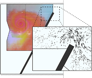
The experiments were conducted in the directional wave basin of Oregon State University, the size of which measures  $44\ \textrm {m}\times 26.5\ \textrm {m}$ in plan-view (figure 1). A physical configuration, in the image of a port entrance, was created by building a breakwater across the basin at a $27^{\circ }$ angle with respect to the wavemaker. A gap of width ${\sim }3.1$ m, formed between the breakwater tip and the basin sidewall, created a nozzle effect and accelerated the flow past it. The 26.5 m long, 0.6 m wide and 0.8 m high breakwater was built using 12 in. $\times$ 8 in. $\times$ 16 in. ( ${\sim } 0.3\ \textrm {m} \times 0.2\ \textrm {m} \times 0.4\ \textrm {m}$) cinder blocks and the sides were covered with white acrylic Plexiglass sheets to create an impermeable and smooth surface.

Figure 1. The experimental set-up in the tsunami wave basin. Grey polygons denote the fields of view of the overhead cameras and the black square denotes the horizontal position of the acoustic Doppler velocimeter (ADV) that was mounted mid-depth in the offshore basin. Figure inset shows the wavemaker displacement time-history, the free surface elevation (FSE) recorded near the wavemaker (position of the corresponding gauge is shown with the black star) and the average velocity across the harbour channel.
The wavemaker of the basin has a maximum stroke of 2 m and maximum velocity of  $2\ \textrm {m}\ \textrm {s}^{-1}$. The wavemaker motion and water level were optimised to generate a stable TCS off the tip of the breakwater. Numerical simulations using the model of Kim & Lynett (Reference Kim and Lynett2011) provided the initial parameters, which were later fine-tuned during preliminary experiments. The finalised uniform piston displacement produced a single asymmetric pulse with a 42 s period, resembling a leading-elevation N-wave (Tadepalli & Synolakis Reference Tadepalli and Synolakis1994) (inset of figure 1). The water level was set at $h = 55$ cm, resulting in a wavelength of ${\sim }98$ m (approximately twice the length of the basin). For a typical prototype harbour channel depth of 15 m and using Froude scaling, the wavelength, period and amplitude translate into a prototype 2.7 km, 3.7 min. and 1 m, respectively, which are all within near-shore geophysical tsunami scales. Thus, this experiment has the rare property of being realistically scaled with respect to both length and time.
The current induced by the small-amplitude, long-period wave was funnelled through the channel. The channel flow rate was strong enough to form separated regions, which when coupled with the near-boundary shear layers (along the breakwater) and transient flow, led to the formation of a TCS. The leading-elevation asymmetric wave initially generated a TCS on the inshore side of the breakwater tip (phase 1, figure 2). Once the wavemaker retreated, and the depression pulse reached the channel, the flow direction started shifting towards the wavemaker. The channel experienced higher current velocities during the return flow, being further reinforced by the reflection of the leading elevation wave off the basin's back wall. The stronger return flow generated the offshore TCS (phase 2, figure 2). No additional waves were generated through the wavemaker creating currents in the channel and advecting the TCS back towards the channel (as is the case for geophysical tsunamis). Thus, the offshore vortex was allowed to gain strength, detach from the trailing jet and eventually evolve as a free TCS in the offshore basin (phase 3, figure 2).

Figure 2. The three experimental phases: (1) the wavemaker forward stroke creates a clockwise-spinning TCS on the inshore basin side; (2) the leading wave gets reflected off the back wall of the basin and the wavemaker retracts to create a reverse current through the channel that generates the anticlockwise-spinning offshore TCS; (3) the offshore TCS detaches from the trailing jet and gets advected (multiple TCSs illustrate the position and size of the experimental TCS at different times).
The boundary layer for this oscillatory flow is not fully turbulent since the start of experimental phases 1 and 2. The Reynolds number that can be used to interpret the boundary layer for turbulent oscillatory boundary-layer flows is  $Re_l=U_ml/\nu$ (Jensen, Sumer & Fredsøe Reference Jensen, Sumer and Fredsøe1989), where $\nu$ is the kinematic viscosity, $U_m$ is the maximum freestream velocity and the length scale $l$ corresponds to the amplitude of the freestream motion (equal to $U_m/\omega$ if the freestream velocity varies sinusoidally, where $\omega$ is the angular frequency of the motion). For this experiment, the length scale $l$ is equal to the wavemaker displacement of 1 m (half the stroke) near the wavemaker but becomes much longer in the harbour channel due to flow confinement in the narrow channel. The average velocity in the harbour channel (inset of figure 1) shows that the wave is asymmetric, and therefore the amplitude of the freestream motion $l$ is computed for each of the two TCS-generation phases separately. Here $l$ is defined as one half of the integral of the channel-averaged velocity between the start and end of each phase and the maximum freestream velocity is defined as $U_m=l{\rm \pi} /T_{1/2}$, where $T_{1/2}$ is the half-period (time between the start and end of each phase). These are found to be $l_1 = 4.5$ m, $U_{m1} = 0.45\ \textrm {m}\ \textrm {s}^{-1}$ and $l_2 = 6.9$ m, $U_{m2} = 0.58\ \textrm {m}\ \textrm {s}^{-1}$ for phases 1 and 2, respectively, and (using $\nu =10^{-2}\ \textrm {cm}^{2}\ \textrm {s}^{-1}$) the corresponding Reynolds numbers are $Re_{l1} = 2.0\times 10^{6}$ and $Re_{l2} = 4.0\times 10^{6}$, respectively. The boundary layer during phase 1 becomes turbulent at $\omega t \approx 30^{\circ }$ (within 5.3 s after $t = 9$ s, or $t \sim 14.3$ s of the experiment) and the boundary layer during phase 2 becomes turbulent at $\omega t \approx 20^{\circ }$ (within 4.2 s after $t = 40.6$ s, or $t \sim 44.8$ s of the experiment) (inferred from figure 8 of Jensen et al. (Reference Jensen, Sumer and Fredsøe1989)).
The flow properties that led to the generation of the inshore and offshore coherent structures during the experimental time period  $t=0\text {--}76$ s, where $t$ represents time, are described in detail in Kalligeris (Reference Kalligeris2017). Vorticity maps during the offshore TCS generation (phase 2) are shown in figure 3. The generation phase of the offshore TCS initially starts as a dipole, and the inshore TCS carrying negative vorticity is advected along the top basin wall. The front of the inshore TCS is moving faster than the front of the offshore TCS and begins surrounding it through the front at $t\sim 55$ s. This process can be visualised through the images taken during experiments using dye shown in figure 4, with the negative vorticity carried by the red-coloured fluid. The two counter-rotating fluid volumes interact with each other creating a meandering pattern along the perimeter of the offshore TCS, and the inshore TCS eventually gets integrated into the offshore TCS's ring of support of negative-signed vorticity. The offshore TCS carrying positive vorticity reaches its maximum strength at $t\sim 55$ s, after which point the TCS circulation is intermittently re-enhanced by merging with secondary vortices shed from the trailing jet. The offshore TCS separates from the trailing jet at $t\sim 76$ s, as determined from visual inspection of figure 4.

Figure 3. Vorticity ( $\omega _z$) maps during the offshore TCS generation showing the inshore and offshore TCSs carrying negative and positive vorticity, respectively. Dashed contours designate negative vorticity, plotted every $-0.2\ \textrm {s}^{-1}$ starting from $-0.2\ \textrm {s}^{-1}$, and continuous contours designate positive vorticity, plotted every $0.2\ \textrm {s}^{-1}$ starting from $0.2\ \textrm {s}^{-1}$. The offshore TCS-centre (blue circles) was defined as the centre of mass of the vorticity contour $0.7 \times \omega _{z,max}$, with $\omega _{z,max}$ computed after setting vorticity values near the breakwater tip (within the black circles) to zero. After Kalligeris (Reference Kalligeris2017).

Figure 4. Images from a dye visualisation experiment captured from an oblique angle during the offshore TCS generation phase. Fluorescent green dye is released from the breakwater tip (inside the separation zone) and fluorescent red dye is released just inshore of the tip carrying negative-signed vorticity. Areas of high image intensity correspond to overhead light reflections on the water surface. After Kalligeris (Reference Kalligeris2017).
The results presented in this work are concerned with the evolution of the offshore monopolar vortex after its formation (phase 3, figure 2). The time period examined corresponds to  $t=70\text {--}3000$ s, allowing for some overlap with the TCS-generation analysis (Kalligeris Reference Kalligeris2017). The velocity field is represented in a TCS-centred coordinate system which accounts for the variation in the TCS-centre paths observed in the experimental trials.
2.2. Measurements of 2-D surface flow fields
Four overhead cameras mounted on the basin's ceiling were used to visually capture the water surface at  $29.97$ frames per second in high-definition resolution ( $1920 \times 1080$ pixels). The water surface was seeded with surface tracers in order to measure the free surface flow field through particle tracking velocimetry (PTV) analysis. The surface tracers used were spherical with 4 cm diameter and made of polyplastic, each weighing $2.7\times 10^{-2}\ \textrm {kg}$. The tracer's mass, excluding surface tension, translates to a tracer submergence depth of 7 mm and a submerged centre of mass at ${\sim }2$ mm from the free surface. While local turbulence intermittently affected the tracers’ submergence depth (mostly during phases 1, 2 and early phase 3), the tracers were clearly visible by the cameras at all times. The black-coloured tracers were regularly coated with a hydrophobic material that was partially successful in preventing tracers from conglomerating due to surface tension, and any tracers that conglomerated were excluded from the analysis. The floor and sidewalls of the basin were painted white to maximise the contrast with the tracers.
Maximising coverage of the basin study area necessitated minimising the overlap between the camera fields of view (grey polygons in figure 1). Since the camera fields of view were not overlapping, spatial information could only be extracted in the two horizontal dimensions. The camera set-up was such to achieve at least 6 pixels per particle diameter resolution at the water surface ( $1.5\ \textrm {pixels}\ \textrm {cm}^{-1}$ for the $\sigma = 4\ \textrm {cm}$ diameter tracers), which is an adequate resolution for the tracer-centre detection and PTV algorithm of Crocker & Grier (Reference Crocker and Grier1996) used here (implemented through the MATLAB toolbox of Kilfoil & Pelletier (Reference Kilfoil and Pelletier2015)). The tracer interframe displacement error created a jitter in the velocity time seriesof the tracers with magnitude up to ${\sim }0.025\ \textrm {m}\ \textrm {s}^{-1}$ in each direction. This fluctuation was removed by filtering the velocity time series of each tracer using a low-pass Butterworth filter with a 0.75 Hz cutoff frequency. The present study does not examine the turbulent properties of the flow and therefore filtering (turbulent) motions of frequency higher than 0.75 Hz has no impact on the mean flow properties presented.
The direct linear transformation equations (known as DLT equations) (Holland et al. Reference Holland, Holman, Lippmann, Stanley and Plant1997) were used to convert the image coordinates of the tracer-centres to world (Cartesian) coordinates, and finally the velocity vectors were extracted in physical units using the backward finite-difference scheme. The PTV experiments were repeated 22 times to confirm repeatability of the experiment and collectively obtain a satisfactory density of data. Details on the experimental set-up and the methods used for the velocity data extraction can be found in Kalligeris (Reference Kalligeris2017).
2.3. Coordinate transformation
Studying the TCS evolution requires the coordinate system to be referenced to the TCS-centre, i.e. in polar coordinates. The transformation of the position  $\boldsymbol {X}=(x,y)$ and the corresponding velocity components ( $u,v$) of the scattered velocity vectors extracted from PTV is given by
 \begin{align} r=\|\boldsymbol{X} - \boldsymbol{X}_c \|, \quad \theta=\arctan\left( \frac{y-y_c}{x-x_c}\right), \quad \begin{bmatrix} u_r \\ u_{\theta} \end{bmatrix}= \begin{bmatrix} \cos(\theta) & \sin(\theta) \\ -\sin(\theta) & \cos(\theta) \end{bmatrix} \begin{bmatrix} u \\ v \end{bmatrix}, \end{align}
where  $\boldsymbol {X}_c=(x_c,y_c)$ is the TCS-centre position, and $(r,\theta )$ and $(u_r,u_{\theta })$ are the coordinates and velocity components along the radial and azimuthal directions, respectively. This coordinate transformation allows for the velocity vectors from individual trials to be tied to a common spatial reference. Typically, the vortex centre is identified via $\lambda _2$, $\lambda _{ci}$ (swirl strength), or vorticity operator maps (e.g. Jeong & Hussain Reference Jeong and Hussain1995; Adrian, Christensen & Liu Reference Adrian, Christensen and Liu2000; Seol & Jirka Reference Seol and Jirka2010). The local extrema of these operators in principle define the centre of flow rotation, provided the velocity field is well resolved.
The remapping of the velocity field on a regular grid has proved to be a challenging task for this experiment. In the early stages of the TCS development, the flow around the TCS-centre was characterised by a distinct zone of flow convergence near the centre, followed by a flow-divergence zone at larger radii. As a result, tracers either conglomerated in the TCS-centre or diverged away from it, thus forming a ring of sparse tracer density which affected the data sampling distribution for spatial interpolation. Even when the flow was well-seeded at the time of TCS generation, the density of tracers was significantly reduced within  ${\sim }30$ s. Consequently, the TCS-centre was identified using both vorticity maps – useful as long as the density and spatial distribution of tracers produced an accurate representation of the metric – and by tracking the centre of mass of the conglomerated tracers at the TCS-centre. The procedure for identifying the TCS-centre is detailed in appendix A. Figure 5 shows the resulting TCS-centre paths of all the individual trials, which provided the basis for the coordinate transformation of the PTV-extracted velocity vectors. The TCS-centre in each trial followed a slightly different path due to the chaotic nature of fully turbulent flows.

Figure 5. The TCS-centre paths recorded in each of the experimental trials (grey lines). Arrival times are stated at selected TCS-centre locations (solid squares) for one of the experimental trials. The maximum circle fitting the polygon defined by the solid boundaries is shown with the dashed line. Its centre lies in the location shown with the solid black circle.
2.4. TCS-centre velocity
The TCS-centre velocity provides the means to represent the velocity field in a frame moving with the TCS-centre (e.g. Flór & Eames Reference Flór and Eames2002) and was computed from the filtered TCS paths of the individual experimental trials (figure 6a,b). The individual velocity time series appears noisy due to the inaccuracies involved in determining the TCS-centre through the vorticity maps of sparse velocity vectors. To increase the confidence level of the estimation, the mean TCS-centre velocity time-history was used instead of the individual realisations. The standard error of the both the  $u$- and $v$-velocity expected values, computed as $SEM=\sigma /\sqrt {n}$, where $\sigma$ is the standard deviation of the sample and $n$ is the number of realisations, becomes less than $1\ \textrm {cm}\ \textrm {s}^{-1}$ after 54 s. The resulting mean TCS-centre velocity at each time step was subtracted from the corresponding instantaneous velocity field of each trial.

Figure 6. The TCS-centre velocity in the  $x$- (a) and $y$-directions (b) for all experimental trials (light grey lines) and the mean (thick black).
2.5. TCS-centred ensemble
An ensemble flow field was created from the instantaneous surface velocity vectors of the individual experimental trials (figure 7) for every video frame (at  ${\sim }30$ Hz) to study the flow field around the TCS-centre using an adequate velocity vector resolution. The spatial domain extent of the ensemble is limited in radius to the closest vertical boundary of the basin. This distance, $d_{min}$, represents the maximum possible radius the TCS may attain. At any given time step ( $i$),
$i$),  $d^{i}_{min}$ is defined as the global minimum of the minimum distances ( $d^{i}_j$) between the TCS-centres $({\boldsymbol X}_{cj}^i)$ of the individual trials ( $j=1\ldots N_{trials}$) and the closest vertical boundary ( $\partial \boldsymbol {B}$) as
 \begin{equation} d^{i}_{min}=\underset{j=1\ldots N_{trials}}{{\min}} \left\{ d^{i}_j \right\}= \underset{j=1\ldots N_{trials}}{{\min}} \left\{ \| {\boldsymbol X}_{cj}^i -\partial \boldsymbol{B} \|_{min} \right\}, \end{equation}
where the boundary  $\partial \boldsymbol {B}$ corresponds to the offshore basin perimeter, defined by the sidewalls, breakwater and retracted wavemaker.

Figure 7. Assembly of the TCS-centred ensemble using the surface velocity vectors of all the available individual experimental trials referenced to the TCS-centre (black circles) – example shown for the time instant of  $t=90$ s using velocity vectors from 19 experimental trials.
2.5.1. Azimuthal-averaged profiles
It is useful to examine the properties of the TCS flow field through azimuthal-averaged profiles, although the experimental data show that it is not strictly axisymmetric; the current through the harbour channel induced flow asymmetry in the early stages of TCS development ( $t<150$ s). For the ( $u_r,u_{\theta }$) velocity components, annuli were employed as interrogation windows, averaging along the azimuthal direction all velocity vectors located inside each annulus. Annuli spaced at ${\rm \Delta} r=0.25$ m with 50 % overlapping were found to satisfy the Nyquist criterion ( ${\rm \Delta} r \geqslant 2 \delta _r$) dictated by the average spacing of the vectors $\delta _r$ in the radial direction.
The computation of vertical vorticity  $\omega _z$, hereafter symbolised as $\omega$, typically requires evaluation of the velocity field on a regular grid and the application of a finite difference scheme. The TCS-centred ensemble domain, with spatial extent $x,y \in [-d^{i}_{min},d^{i}_{min}]$, was discretised into nodes of regular spacing ${\rm \Delta} x={\rm \Delta} y=0.4$ m, on which the mean velocity field was evaluated by averaging all velocity vectors within an interrogation window of radius $W_R=0.4$ m – the number of contributing trials and mean tracer spacing in the evaluation domain ( $\delta ^{i}=\sqrt {A^{i}/N_{tracers}^{i}}$, where $A^{i}$ and $N_{tracers}^{i}$ are the area of the evaluation domain and number of tracers within that area for time step (i)) are plotted in figure 8(a) with the mean tracer spacing ranging from $14$ cm at $t=100$ s, when the number of contributing trials was high, to $40$ cm at $t=3000$ s. Velocity vectors in nodes with sparse tracer distribution ( $N<4$), were obtained using the natural-neighbour interpolation scheme (e.g. Lloyd, Stansby & Ball Reference Lloyd, Stansby and Ball1995). Vorticity was evaluated on the regular grid nodes using the four-point, second-order accurate, least-square differential operator (Raffel et al. Reference Raffel, Willert, Wereley and Kompenhans2007). Converting the regular grid nodes to polar coordinates does not result in constant radial spacing. Therefore, for the purpose of obtaining azimuthal-averaged vorticity profiles, the vorticity maps were subsequently interpolated on concentric nodes using constant radial spacing $\textrm {d}r=W_R=0.4$ m and a radius-dependent step $\textrm {d}\theta$ in the azimuthal direction
 \begin{equation} \textrm{d}\theta(r)=2\arcsin \left( \frac{\textrm{d}r}{2r} \right), \end{equation}
in what here is called the concentric grid. Finally, the vorticity profiles were obtained by azimuthal-averaging the vorticity values at the nodes corresponding to each radius. The benefit of interpolating the vorticity values from the regular grid to the concentric grid nodes using a radius-dependent step  $\textrm {d}\theta$ is that the spacing between the regular and concentric grid nodes is comparable, and thus any additional distortion of the vorticity field due to spatial interpolation is minimised.

Figure 8. (a) Mean tracer spacing in the domain extending to  $x,y \in [-d^{i}_{min},d^{i}_{min}]$ and the number of experimental trials contributing to the ensemble (grey bars). (b) Vorticity decay near the TCS-centre as measured from the two tracer configurations (shown in the inset) that were only used in dedicated experimental trials to measure vorticity (§ 2.6). The dashed and continuous lines correspond to the low-pass filtered vorticity measured using the cross-tracer in two different experimental trials, and the dash-dot line to the square tracer. The dark and light grey lines are the raw vorticity curves of the cross-tracer and the square tracer, respectively.
2.6. Direct measurements of vertical vorticity
Surface-tracer configurations were used to track the local flow rotation and infer vorticity near the TCS-centre in dedicated experimental trials (with no other tracers in the flow field). The two configurations that were tested are shown in the inset of figure 8(b). Both were made out of four surface tracers constituting the vertices of a square. In the first configuration, the sides are interconnected (square tracer), whereas in the second the diagonals are interconnected to form a cross (cross-tracer). The cross-tracer was used in two experimental trials, whereas the square tracer was introduced in the flow only for one experimental trial. The tracer configurations merged to the TCS-centre, with the four vertices spinning approximately around it.
The vertices of the tracer configurations were tracked using the 2-D PTV method described in § 2.2. The centre of mass of each configuration defined the centre of a local polar coordinate system  $(r,\theta )$. The angular velocity of each vertex $i$, at time step $j$ was computed using the backward finite difference scheme
 \begin{equation} \varOmega_i^{j}=\frac{\theta_i^{j}-\theta_i^{\,j-1}}{t^{j}-t^{\,j-1}}=\left( \frac{\textrm{d}\theta}{\textrm{d}t}\right)_i^{j}. \end{equation}
The instantaneous vorticity shown in figure 6(c) was computed as
 \begin{equation} \omega^{j}=2 \langle \varOmega_{i=1:4}^{j}\rangle, \end{equation}
since  $u_{\theta }=r \varOmega$, and the vertical vorticity for solid-body rotation and axisymmetric flow is given by $\omega (r) = {1}/{r}(u_{\theta }+r({\partial u_{\theta }}/{\partial r}))={1}/{r}(r \varOmega +r({\partial (r \varOmega )}/{\partial r}))=2 \varOmega$.
The fluctuation in the vorticity time series shown in figure 8(b) is a result of the off-centre rotation and the translating motion of the tracers (see appendix A). The low-pass filtered vorticity time series for the two cross-tracer trials match well (figure 8b), justifying the repeatability of the experiment using tracer configurations. The vorticity offset in the decay curves for the two different configurations is due to the difference in the radial distance to the vertices.
2.7. Mid-depth ADV measurements
A Nortek Vectrino ADV was mounted near mid-depth ( $z=0.271$ m) in the offshore basin (figure 1), sampling four velocity components at 50 Hz frequency: horizontal velocities $u$,
$u$,  $v$, and $w_1$ and $w_2$, where $w_1$ and $w_2$ are independent and redundant measurements of the vertical velocity. Four experimental trials included the ADV, after which it was removed since its mounting was found to be affecting the path of the offshore TCS. The horizontal velocity components from the experimental trial resulting in the highest correlation are shown in figure 9(a,b).

Figure 9. (a,b) Comparison between horizontal velocities extracted from the ADV (located at  $x=4.52$ m, $y = 0.01$ m, $z=0.271$ m) and the corresponding velocities extracted from PTV analysis – values sampled at 3 Hz. (c–e) Statistics for the differences between the two data-sets corresponding to the time interval $0 \leqslant t \leqslant 150\,{\rm s}$.
The PTV velocity vectors were sampled from all the 22 experimental trials described in § 2.2 to create an ensemble flow field in Cartesian coordinates; however, the ensemble used in this section was not referenced to the TCS-centre. The PTV-extracted velocity components from the nearest tracer to the ADV are plotted against the ADV-extracted velocities in figure 9(a,b), with both time series sampled at 3 Hz. The time series compare well for  $t \leqslant 150$ s, while the velocity deviation for $t>150$ s can be attributed to the TCS path which starts to affect the free surface elevation at the location of ADV1 – different experimental realisations can lead to different TCS-centre paths.
For a turbulent boundary layer, the relation between free surface and mid-depth velocity can be estimated using the logarithmic velocity profile relating the streamwise velocity  $u$ at elevation $z$ above the bed with the bed shear velocity $u_*$
$u_*$
 \begin{equation} \frac{u}{u_*}=\frac{1}{\kappa}\log\left(\frac{z}{z_0}\right), \end{equation}
where  $\kappa =0.4$ is the Karman constant and $z_0$ is the bed roughness length. For open channel flows, the logarithmic profile typically holds true for $z/h<0.2$ and also approximates the profile well for $0.2<z/h<0.7$ (Cardoso, Graf & Gust Reference Cardoso, Graf and Gust1989). In open channels with uniform flow, the logarithmic profile may extend until $z=\beta h$ and the velocity remains constant for $z>\beta h$, with $\beta \sim 0.7$ being a typical value (Le Coz et al. Reference Le Coz, Hauet, Pierrefeu, Dramais and Camenen2010).
Assuming the logarithmic profile extends to the free surface, provides the highest expected deviation between the free surface-extracted velocity and any other velocity value along the water column. Using a bed roughness length for a hydraulically smooth flow  $z_0 \approx 0.135\nu /u_*$ and $u_*\approx U\sqrt {c_f/2}$, where $c_f$ is the the bed friction coefficient and $U$ is the depth averaged velocity, $c_f=0.01$ (§ 4.3) and $U$ ranging between $0.01\text {--}0.5\ \textrm {m}\ \textrm {s}^{-1}$, (2.6) yields a maximum expected $u_{ptv}/u_{adv}$ ratio ranging between 1.06–1.10. Using the same assumptions, the corresponding maximum expected $u_{ptv}/U$ ratio for a turbulent boundary layer ranges between 1.09–1.14.
Statistics of the comparison between the ADV- and PTV-extracted horizontal velocities are presented in figure 9(c–e). The metrics presented were computed for the time interval  $0 \leqslant t \leqslant 150$ s using a 3 Hz sampling frequency, i.e. 450 total counts. The $u_{ptv}$ and $v_{ptv}$ values are generally smaller and larger than $u_{adv}$ and $v_{adv}$, respectively (figure 9c,d). Half and 91 % of the values of $u_{ptv}-u_{adv}$ are within ${\pm }0.0065$ and ${\pm }0.02\ \textrm {m}\ \textrm {s}^{-1}$, whereas half and 96 % of the $v_{ptv}-v_{adv}$ lie within ${\pm } 0.005$ and ${\pm } 0.02\ \textrm {m}\ \textrm {s}^{-1}$, respectively. Half the values of the velocity magnitude difference ( $\sqrt {u_{ptv}^{2}+v_{ptv}^{2}}-\sqrt {u_{adv}^{2}+v_{avd}^{2}}$) are within ${\pm }0.006\ \textrm {m}\ \textrm {s}^{-1}$ and 91 % are within ${\pm }0.02\ \textrm {m}\ \textrm {s}^{-1}$ (figure 9e). While 62 % of the PTV velocity magnitude sample values extracted at the free surface are larger than the velocity magnitude measured by the ADV mid-depth, it is not possible to precisely quantify the ratio between the two since the two data-sets do not correspond to the same experimental trial.
2.8. FSE measurements -- basin response
Free surface elevation data were collected throughout the basin for 30 min at 50 Hz sampling frequency using resistance wave gauges mounted on the basin's instrumentation bridge (more details on FSE data collection are provided in appendix B). The collected FSE time series are used in this section to examine the sloshing wave motions that took place inside the basin during the experiments. As the experimental TCS were evolving in the offshore basin, the sloshing motions produced a pulsating radial velocity that could be traced in the PTV-extracted velocities (see § 5.2). This analysis is useful in confirming that the pulsating radial velocity signal is a result of basin resonance.
Wave energy spectra  $S_i(\,f)$ for each surface elevation time series in the offshore basin were computed through fast Fourier transformation analysis. Common energy peaks were identified from the space-averaged wave spectrum given by
 \begin{equation} \bar{S}(\,f)=\frac{1}{N}\sum_{i=1}^{N}S_i(\,f), \end{equation}
where  $N$ is the number of wave gauges in the offshore wave basin. The space-averaged spectrum provides a means to readily examine the frequencies that contain the most energy in the basin. The frequency of each significant energy peak in the space-averaged spectrum represents a resonant basin frequency ( $\,f_r$), i.e. a sloshing motion. The spatial distribution of spectral energy in each of the resonant frequencies corresponds to the resonant modes, visualised here by interpolating the point values of spectral energy in the offshore wave gauge locations using a biharmonic spline interpolation scheme (Sandwell Reference Sandwell1987).
The space-averaged spectrum and the first six resonant modes are shown in figure 10. What appears to be the fundamental resonant mode (Rabinovich Reference Rabinovich2010) of the whole basin is traced at  $1/\,f_r=78.8$ s, whereas the fundamental mode of the offshore basin alone is traced at $1/\,f_r=23.1$ s. The higher resonant modes involve more antinodes at different locations. Note that the mode plots capture the presence of the TCS, most notably near the top basin wall where the TCS experienced high local depressions at the free surface (see § 4.4).

Figure 10. (a) Space-averaged wave energy spectrum and identified resonant frequencies (grey circles). (b–g) The sloshing modes of the offshore wave basin corresponding to the resonant frequencies. The colourmaps are normalised using the maximum spectral energy  $S(\,f_r)_{max}=\max [S_i(\,f_r)]_{i=1}^{N}$ corresponding to each resonant frequency $f_r$, stated as $M$ in each subplot ( $M=S_{max}$, given in units of $\textrm {m}^{2}\ \textrm {s}$).
3. Theoretical analysis for shallow TCS
3.1. Governing equations
Turbulent shallow water flows with large horizontal to vertical scale ratios ( $L/H\gg 1$) imply the hydrostatic approximation. Thus, Q-2-D vortex structures are often modelled using the depth-averaged shallow-water equations (Seol & Jirka Reference Seol and Jirka2010). For a 2-D turbulent flow with surface elevation $\eta (r,\theta ,t)$ over an undisturbed water-depth $h(r,\theta )$ and no background rotation, of a fluid with density $\rho$, the depth-averaged incompressible continuity equation and equations of motion are given in cylindrical coordinates by
 \begin{gather} \frac{\partial \eta}{\partial t}+\frac{1}{r}\frac{\partial(r \,\textrm{d} \bar{u}_r)}{\partial r}+\frac{1}{r} \frac{\partial(\textrm{d}\bar{u}_{\theta})}{\partial \theta}=0, \end{gather}
 \begin{align} &\frac{\partial \bar{u}_r}{\partial t}+\bar{u}_r\frac{\partial\bar{u}_r}{\partial r}+\frac{\bar{u}_{\theta}}{r} \frac{\partial \bar{u}_r}{\partial \theta} - \frac{\bar{u}_{\theta}^{2}}{r}=-\frac{1}{\rho}\frac{\partial p}{\partial r}+\nu_{eff}\left[\frac{1}{{d}} \frac{\partial {d}}{\partial r}\frac{\partial \bar{u}_r}{\partial r}+\frac{\partial}{\partial r} \left(\frac{1}{r} \frac{\partial (r\bar{u}_r)}{\partial r} \right)\right.\nonumber\\ &\left.\quad+\frac{1}{r^{2}}\left( \frac{1}{{ d}}\frac{\partial}{\partial \theta}\left({ d} \frac{\partial \bar{u}_r}{\partial \theta}\right)-\frac{1}{{ d}}\frac{\partial ({ d} \bar{u}_{\theta})}{\partial \theta}-\frac{\partial \bar{u}_{\theta}}{\partial \theta} \right) \right]- \frac{\tau_{zr}(-h)}{\rho d}, \end{align}
 \begin{align} &\frac{\partial \bar{u}_{\theta}}{\partial t}+\bar{u}_r\frac{\partial\bar{u}_{\theta}}{\partial r}+\frac{\bar{u}_{\theta}}{r} \frac{\partial\bar{u}_{\theta}}{\partial \theta}+\frac{\bar{u}_{\theta} \bar{u}_r}{r}=-\frac{1}{r\rho}\frac{\partial p}{\partial \theta}+ \nu_{eff}\left[\frac{1}{{ d}}\frac{\partial { d}}{\partial r}\frac{\partial \bar{u}_{\theta}}{\partial r}+ \frac{\partial}{\partial r} \left(\frac{1}{r} \frac{\partial (r\bar{u}_{\theta})}{\partial r} \right)\right.\nonumber\\ &\quad \left.+\frac{1}{r^{2}}\left( \frac{1}{{ d}}\frac{\partial}{\partial \theta}\left({ d} \frac{\partial \bar{u}_{\theta}}{\partial \theta}\right)+\frac{1}{{ d}}\frac{\partial ({ d} \bar{u}_r)}{\partial \theta}+\frac{\partial \bar{u}_r}{\partial \theta} \right) \right]-\frac{\tau_{z \theta}(-h)}{\rho d}, \end{align}
where  $d$ is the total water depth ( $d=h+\eta$), and $\bar {u}_r,\bar {u}_{\theta }$ are the depth-averaged horizontal velocities. Here $\nu _{eff}$ is the effective viscosity, given as the sum of turbulent and molecular kinematic contributions: $\nu _{eff}=\nu _{turb}+\nu$, thus adding more dissipation/diffusion to the flow description due to turbulence. For an axisymmetric flow ( $\partial /\partial \theta =0$) over a flat surface ( $\partial h/\partial r,\partial h/\partial \theta =0$), the governing equations are reduced to
 \begin{gather} \frac{\partial \eta}{\partial t}+\frac{1}{r}\frac{\partial(r \,\textrm{d} \bar{u}_r)}{\partial r}=0, \end{gather}
 \begin{gather}\frac{\partial \bar{u}_r}{\partial t}+\bar{u}_r\frac{\partial\bar{u}_r}{\partial r} - \frac{\bar{u}_{\theta}^{2}}{r}=-\frac{1}{\rho}\frac{\partial p}{\partial r}+\nu_{eff}\left[\frac{1}{d}\frac{\partial \eta}{\partial r}\frac{\partial \bar{u}_r}{\partial r}+\frac{\partial}{\partial r} \left(\frac{1}{r} \frac{\partial (r\bar{u}_r)}{\partial r} \right) \right]-\frac{\tau_{br}}{\rho d}, \end{gather}
 \begin{gather}\frac{\partial \bar{u}_{\theta}}{\partial t}+\bar{u}_r\frac{\partial\bar{u}_{\theta}}{\partial r}+\frac{\bar{u}_{\theta} \bar{u}_r}{r}=\nu_{eff}\left[\frac{1}{d}\frac{\partial \eta}{\partial r}\frac{\partial \bar{u}_{\theta}}{\partial r}+\frac{\partial}{\partial r} \left(\frac{1}{r} \frac{\partial (r\bar{u}_{\theta})}{\partial r} \right) \right]-\frac{\tau_{b\theta}}{\rho d}. \end{gather}
Henceforth all velocities stated correspond to depth-averaged quantities and the bar will be omitted to simplify the notation.
The added viscosity due to turbulence can be modelled using the Elder (Reference Elder1959) formula expressed in terms of the bed friction coefficient
 \begin{equation} \nu_{eff} \approx \nu_{turb} \approx u_* h \approx \sqrt{\frac{c_f}{2}} U h, \end{equation}
where  $U$ is a reference horizontal velocity (Seol & Jirka Reference Seol and Jirka2010); typical values for the bed friction coefficient $c_f$ are $c_f\approx 0.005,0.01$ for the field and laboratory, respectively (Socolofsky & Jirka Reference Socolofsky and Jirka2004). The $\nu _{eff}$ terms of the momentum equations represent lateral turbulent diffusion. Vertical diffusion due to the no-slip boundaries is represented by the bottom shear stress terms $\tau _{bx},\tau _{by}$, which are computed using the quadratic friction law
 \begin{equation} \tau_{br}=\rho \frac{c_f}{2}u_r\sqrt{u_r^{2}+u_{\theta}^{2}},\quad \tau_{b\theta}=\rho \frac{c_f}{2}u_{\theta}\sqrt{u_r^{2}+u_{\theta}^{2}}. \end{equation}
3.2. Monopolar vortex theory
This section summarises the governing equations for a purely azimuthal vortex flow with no background rotation. As long as the secondary flow components (radial and vertical velocities) are strong, it is expected that the assumptions of axisymmetry and purely azimuthal flow will be violated. The deviation from the theory will provide a basis to quantify the effect of the secondary flow on the main (2-D) vortex structure.
Assuming a purely azimuthal flow ( $u_r,\tau _{br}=0$) with no background rotation, the radial component of the depth-averaged cylindrical Navier–Stokes equations (3.5) is reduced to the cyclostrophic balance equation
 \begin{equation} \frac{u_{\theta}^{2}}{r}=\frac{1}{\rho}\frac{\partial p}{\partial r}. \end{equation}
Further assuming that  $h\gg \eta$ (thus $d\approx h$), and substituting for $\nu _{eff}$ and $\tau _{b\theta }$ using (3.7) and (3.8a,b), the momentum equation in the azimuthal direction (3.6) becomes
 \begin{equation} \frac{\partial u_{\theta}}{\partial t}=\sqrt{\frac{c_f}{2}} u_{\theta} h \left[\frac{1}{h}\frac{\partial \eta}{\partial r}\frac{\partial u_{\theta}}{\partial r}+\frac{1}{r}\frac{1}{\partial r} \left(r \frac{\partial u_{\theta}}{\partial r} \right)-\frac{u_{\theta}}{r^{2}} \right]-\frac{c_f u_{\theta}^{2}}{2h}, \end{equation}
which corresponds to the radial diffusion equation for fully turbulent flows. The radial diffusion equation for laminar flows is a linear partial differential equation, and the azimuthal velocity profile has been derived analytically using separation of variables and assuming a Poiseuille velocity profile (Satijn et al. Reference Satijn, Cense, Verzicco, Clercx and van Heijst2001). While (3.10) is a nonlinear partial differential equation for which an analytical solution is not known, the temporal dependence can be inferred by assuming that bottom friction dominates over turbulent diffusion (Seol & Jirka Reference Seol and Jirka2010), for which (3.10) reduces to
 \begin{equation} \frac{\partial u_{\theta}}{\partial t}=-\frac{c_f u_{\theta}^{2}}{2h}. \end{equation}
Separation of variables (assuming  $u_{\theta }(r,t)=\xi (r)\psi (t)$) leads to a temporal azimuthal-velocity dependence for $\xi =1$ of the form
 \begin{equation} \psi(t)=\frac{1}{\dfrac{1}{\psi_0}+\dfrac{c_f}{2h}t}. \end{equation}
 The choice of initial conditions for the velocity profile depends on the vortex generation mechanism. Typical profiles for geophysical vortices include the Lamb–Oseen and  $a$-profile (van Heijst & Clercx Reference van Heijst and Clercx2009). The $a$-profile (or isolated) vortex, which is of interest for this particular application, has a fitting dimensionless azimuthal profile of the form (Flór & Van Heijst Reference Flór and Van Heijst1996)
 \begin{equation} \hat{u}_{\theta}(\hat{r})=\hat{r}\exp \left(\frac{1-\hat{r}^{a}}{a} \right), \end{equation}
where  $\hat {u}_{\theta }$ is non-dimensionalised using the maximum azimuthal velocity ( $\hat {u}_{\theta }=u_{\theta }/u_{\theta ,max}$) and the radial distance by the radial distance $R_{v_{max}}$ corresponding to $u_{\theta ,max}$, as $\hat {r}=r/R_{v_{max}}$. The parameter $a$ controls the shape of the profile – the steepness increases with increasing $a$. Stability analysis on this family of isolated vortices has shown that the profile becomes unstable for $a>2$ (Carton, Flierl & Polvani Reference Carton, Flierl and Polvani1989). The corresponding vorticity profile for axisymmetric flow is given by
 \begin{equation} \omega(\hat{r})=\omega_{max} \left(1-\frac{1}{2} \hat{r}^{a} \right) \exp \left(-\frac{\hat{r}^{a}}{a} \right), \end{equation}
where  $\omega _{max}$ can be expressed as $\omega _{max}=2u_{\theta ,max} \exp (1/a)/R_{v_{max}}$, and $\omega$ becomes zero at radius $r=R_{v_{max}}2^{1/a}$.
It has been shown that any vortex with some level of axisymmetry and zero initial circulation will eventually evolve into an isolated-type vortex profile (Kloosterziel Reference Kloosterziel1990), and that it is impossible to generate a monopolar vortex of single-signed vorticity (Satijn et al. Reference Satijn, Cense, Verzicco, Clercx and van Heijst2001). The  $a$-profile geophysical vortices have zero circulation ( $\varGamma$), which can be shown by evaluating $\varGamma =\int _0^{\infty } r \omega (r)\,\textrm {d}r$ for any $a$ value.
4. Azimuthal-averaged flow properties
4.1. Mean flow profiles
In this section, the azimuthal-averaged properties of the experimental TCS are presented and analysed, which filter out non-axisymmetric features in the 2-D flow fields. Selected azimuthal-averaged  $u_{\theta }$, $u_r$ and $\omega$ profiles are shown in figure 11 at $300$ s time intervals – the profile radii being limited by the distance to the closest vertical boundary. The azimuthal-averaged profiles are obtained using the procedure outlined in § 2.5.1. The $u_{\theta }$ profiles are normalised by their maxima in the ordinate and the abscissa of all figure 11 subplots is normalised by the radius $R_{v_{max}}$ corresponding to $u_{\theta ,max}$. The ordinate of the vorticity plots is normalised using the vorticity measured at $r=4.9$ cm with the cross-tracer (see figure 8b). It should be noted that for a logarithmic velocity profile along the water column, the PTV-extracted free surface velocity can be up to 14 % larger compared with the depth-averaged values if the logarithmic profile extends to the free surface (§ 2.7). Any such deviation does not affect the use of analytical expressions derived based on depth-averaged velocities to describe the TCS flow field. However, it is expected to impact the best-fitting coefficients based on the free surface velocities presented in this section.

Figure 11. (a–c) Azimuthal velocity ( $u_{\theta }$) profiles normalised with $u_{\theta ,max}$: grey dots correspond to scattered data, error bars to the azimuthal-averaged values and standard deviation, and the dash-dot line to the best-fitting $a$-profile; root mean square error (RMSE) values correspond to the dimensionless RMSE between the normalised best-fitting $a$-profile and scattered data for the radial range shown ( $r/R_{v_{max}} \leqslant 4$). (d–f) Radial velocity ( $u_r$) profiles: grey dots correspond to scattered data, error bars and solid line to the azimuthal-averaged values and standard deviation. (g–i) Azimuthal-averaged vertical vorticity profiles, normalised using the cross-tracer-measured vorticity: the solid line is the azimuthal-averaged vorticity (plotted for $r \geqslant 40$ cm), grey circle and square (and corresponding error bars) denote the cross-tracer and square-tracer-measured vorticity, respectively, the grey dots correspond to the scattered vorticity data evaluated on the regular evaluation grid described in § 2.5.1, and the dash-dot line is the theoretical vorticity profile given by (3.14). The abscissa of all subplots is normalised by $R_{max}$, the radius corresponding to $u_{\theta ,max}$, derived from the best-fitting $a$-profile.
The scattered azimuthal velocity data (grey dots) are fitted to the  $a$-profile defined in (3.13) and the resulting best-fit is shown with the dashed-dot lines at selected times in figure 11(a–c). It can be observed that at early times the azimuthal velocity profiles diverge from $a$-profile. The idealised profile cannot capture the high profile steepness around $u_{\theta ,max}$ and does not account for the change in slope at radii beyond $R_{v_{max}}$. The $u_{\theta }$ profiles start to converge towards the isolated vortex profile at later times, which is evident both qualitatively from the fit, but also quantitatively from the lower RMSE of the fit at $t=500$ s – RMSE increases again at $t=800$ s due to the higher spread of the data points as velocity magnitude decreases. The steepness parameter of the fitted profiles ranges between $a=0.31\text {--}0.43$ throughout the duration of the experiment, which is well below the critical value ( $a<2$).
The maxima of the  $u_r$ velocity profiles are one to two orders of magnitude smaller compared with the $u_{\theta }$ maxima, and exhibit a steady decay with time. Even though the standard deviation of the samples in each evaluation radius is of the same order for both velocity components, the standard deviation as a percentage of the mean (coefficient of variation) is much greater for the radial component. Despite the large uncertainty in the $u_r$ azimuthal-averaging, the profiles serve to visualise the flow divergence patterns. In the early stages of TCS development, the radial velocity profiles indicate a strong convergence zone ( $\partial (r u_r)/\partial r<0$) for $r/R_{v_{max}}<1$. Convergence is followed by a zone of flow divergence in the outer vortex region ( $\partial (r u_r)/\partial r>0$), in agreement with the observations outlined in § 2.3. However, the interpretation of the flow pattern along the radial axis should be cautious since radial velocities extracted from the surface tracers can be affected by the cyclostrophic balance assumption (see appendix C).
The vorticity profiles, at the time steps shown in figure 11 and to the extent of radii considered, do not exhibit negative values but approach the zero contour close to the domain boundary  $d_{min}$. The scattered vorticity data evaluated on the regular grid do not deviate significantly from the azimuthal-averaged data since the ensemble velocity field on the regular grid was averaged within the radius of the interrogation windows (§ 2.5.1). Therefore, the scattered vorticity data points are not representative of the true vorticity fluctuations along the vortex radius. The azimuthal-averaged vorticity profiles match well with the best-fitting $a$-profiles for $r/R_{v_{max}} \geqslant 0.5$, but fail to capture the steep vorticity profile slope closer to the TCS-centre due to the low resolution of the vorticity maps described in § 2.5.1. The experimental vorticity profile was thus cut off at $r=0.4$ m. Instead, vorticity measured through the tracer configuration near the TCS-centre are plotted for $r<0.4$ m, and the measurements compare well with the theoretical $a$-profile.
4.2. TCS radial growth
During the formation stage, the experimental TCS undergoes internal oscillations due to 3-D turbulence. At the same time, the TSC flow structure is merging with vortices shed from the trailing jet (figure 3), periodically gaining circulation. After detaching from the trailing jet, the TCS radius grows due to lateral turbulent diffusion, which can be approximated by
 \begin{equation} R \propto \sqrt{2Et}, \end{equation}
where  $E$ is the diffusivity (Seol & Jirka Reference Seol and Jirka2010). For turbulent conditions, $E$ can be approximated by (Seol & Jirka Reference Seol and Jirka2010)
 \begin{equation} E \approx \nu_{turb} \approx \sqrt{\frac{c_f}{2}} U h, \end{equation}
where  $\nu _{turb}$ is the added viscosity due to turbulence given by (3.7).
The experimental vortex radius can be defined both in terms of the radial distance to the maximum azimuthal velocity, but also in terms of the radial distance to a certain vorticity threshold. The former corresponds to the vortex core radius and the latter to the vortex structure boundary, or bulk radius. The two experimental radii are evaluated through the azimuthal-averaged velocity and vorticity profiles. The vortex core growth  $R_{v_{max}}(t)$ is obtained by fitting the measured $u_{\theta }$ data points to the $a$-profile, whereas the vorticity-defined radius corresponds to the radius $R_{vortex}(t)$ at which $\omega (r,t)=0.02 \omega _{max}(t)$.
The evaluated vortex radii using the above methods are plotted in figure 12(a). The TCS-core growth shows that the vortex core radius remains almost constant until  $t\approx 390$ s, and then follows the $\sqrt {t}$ growth rate; TCS-core growth can be well described by fitting two log–linear segments, as shown in figure 12(a): $R_{v_{max}}=0.95$ m for $70<t<330$ s, and a log–linear segment using a growth rate (slope) $\propto \sqrt {t}$ for $t>330$ s. The vortex bulk radius on the other hand grows as $\sqrt {t}$ since the start of the measurements at $t=100$ s. More specifically, the growth rate follows $\sqrt {t}$ in the time period $t\sim 100\text {--}230$ s. After $t\approx 230$ s, vortex growth is dictated by the distance of the TCS-centre to the vertical boundaries. This shows that the experimental TCS is constantly readjusting its position to allow it to preserve its momentum and continue growing in size by ongoing turbulent diffusion. As the TCS grows, it eventually positions itself at the point in the offshore basin that fits the maximum circle of radius $R_{max}=8.5$ m (figure 5). The TCS-centres in the trials extending to $t\rightarrow 3000$ s reached their final resting position in the offshore basin.

Figure 12. (a) The TCS radial growth with time. Grey squares denote the TCS-core radius, the thin black line is a fit to describe the TCS-core radius growth using two log–linear segments, black circles denote the TCS-bulk radius, and the thick black curve corresponds to the mean-minimum distance to the closest vertical boundary; dashed lines correspond to the viscous diffusion growth rate  ${\sim }\sqrt {t}$. (b) Local depth-based Reynolds number decay of the experimental TCS.
Defining a local depth-based Reynolds number using the maximum azimuthal velocity
 \begin{equation} Re_h(t)=\frac{u_{\theta,max}(t) h}{\nu}, \end{equation}
allows us to characterise the state of the flow (Seol & Jirka Reference Seol and Jirka2010). Figure 12(b) shows the turbulence decay with time (using  $\nu =10^{-2}\ \textrm {cm}^{2}\ \textrm {s}^{-1}$) and confirms that the flow remains well above the Reynolds number corresponding to laminar conditions ( $Re_h\approx 500$). In the outer regions of the vortex flow ( $R_{v_{max}}<r<d_{min}$), $Re_h=u_{\theta }h/\nu$ is $O(10^{4}\text {--}10^{5})$ for $70<t<3000$ s, with the smallest value being $Re_h=16\,813$ for $r=7.75$ m and $t=3000$ s. For The vortex core ( $r<R_{v_{max}}$), an alternative Reynolds number definition can be used $Re_h(t)=\omega _{max}(t) R_{vortex}(t)h/\nu$ (Seol & Jirka Reference Seol and Jirka2010). While the vorticity maps obtained through the PTV data described in § 2.5.1 did not yield the resolution required to evaluate $\omega _{max}$ at the vortex centre, and the direct vorticity measurements near the vortex centre described in § 2.6 did not extend beyond $t>1300$ s, it can be shown through the theoretical definition of $\omega _{max}$ for the $a$-profile $\omega _{max}=2u_{\theta ,max} \exp (1/a)/R_{v_{max}}$ that $\omega _{max}R_{vortex}\gg u_{\theta ,max}$. The vortex flow after detachment from the trailing jet can thus be characterised as fully turbulent for $70<t \leqslant 3000$.
It should be noted that while the measured vortex flow remains turbulent, that is not necessarily true for the flow across the entire wave basin during the course of the experiments. Since all experimental trials involved the same geometrical setting, boundary conditions and water depth, Reynolds number dependence was not examined. However, in the experiments of Seol & Jirka (Reference Seol and Jirka2010), shallow monopolar vortices with initial  $Re_h \geqslant 1.4\times 10^{4}$ and same (strong) shallowness (ratio between initial vortex diameter to water depth) were found to exhibit Reynolds-number-invariant behaviour with large-scale flow features eventually becoming self-similar.
4.3. Vortex decay model
Dimensional analysis of the depth-integrated vorticity equation for large horizontal-to-vertical flow feature scales is able to show that bottom friction dominates over vorticity diffusion for the TCS spin-down and energy decay (Seol & Jirka Reference Seol and Jirka2010). Following the work of Seol & Jirka (Reference Seol and Jirka2010), this section provides a simple force-balance model to match the experimental TCS kinetic energy decay due to bottom friction for turbulent flow.
A force-balance equation can be derived from the local moment of momentum method by equating the rate of angular momentum for a vortex patch of thickness  $\textrm {d}r$ at distance $r$ from the vortex centre to bottom friction $\tau _b$ (Seol & Jirka Reference Seol and Jirka2010)
 \begin{equation} \frac{\textrm{d}}{\textrm{d}r}(r(2{\rm \pi} r h \,\textrm{d}r)u_{\theta})=-r\left(2{\rm \pi} r \,\textrm{d}r \frac{\tau_b}{\rho}\right). \end{equation}
Assuming that the vortex core radius is a constant leads to a force-balance equation for the maximum azimuthal velocity
 \begin{equation} \frac{\textrm{d}}{\textrm{d}t}(h u_{\theta,max})=-\frac{\tau_b}{\rho}, \end{equation}
where  $u_{\theta ,max}$ is the maximum azimuthal velocity at $r=R_{v_{max}}$ (Seol & Jirka Reference Seol and Jirka2010). Substituting for the bottom shear stress for turbulent and purely azimuthal flow (3.8a,b) and integrating leads to
 \begin{equation} u_{\theta,max}(t)=\frac{1}{\dfrac{1}{u_{\theta,max,0}}+\dfrac{c_f}{2h}t}, \end{equation}
where  $u_{\theta ,max,0}=u_{\theta ,max}(t=0)$. Note that the time-dependence of the $u_{\theta ,max}$ decay expression is of the same form as (3.12) that was derived from the momentum equation for a constant radius ( $\xi =1$). Fitting (4.6) to the experimental azimuthal decay data results in a best-fitting $c_f=0.01$ with a RMSE of $9 \times 10^{-4}\ \textrm {m}\ \textrm {s}^{-1}$ (figure 13a). The first-order model captures the physical process of TCS energy decay due to bottom friction very well, showing that the assumption of a slow TCS-core growth is realistic and bottom friction dominates the kinetic energy decay over viscous diffusion.

Figure 13. Decay of TCS mean flow properties compared with the first-order model (dashed lines). (a) Maximum azimuthal (grey circles) and minimum radial (grey dots) velocity decay; maximum azimuthal and minimum radial velocity data points plotted every 50 and 3.3 s, respectively. (b) Azimuthal-averaged vorticity decay evaluated at  $r=R_{v_{max}}$ (grey circles) and prediction $u_{\theta ,max}/R_{v_{max}}$ (dashed line), where $u_{\theta ,max}$ is calculated from (4.6) and $R_{v_{max}}(t)$ is sampled from the TCS-core growth fit using the two log–linear segments shown in figure 12(a); vorticity data points plotted every 50 s.
The  $u_r$ profile minima exhibit an exponential decay as shown in figure 13(a). While this behaviour is compatible with the exponential decay of small-amplitude sloshing waves due to bottom friction (e.g. Dean & Dalrymple (Reference Dean and Dalrymple1991), § 5.6.1), the decay does not show signs of periodicity and thus there is insufficient evidence to support this theory. Instead, $u_r$ minima extracted from the surface tracers are likely capturing the cyclostrophic imbalance between the gravitational and centrifugal forces (appendix C).
The vorticity decay at any radius can be computed by combining (3.14) and (4.6). Of particular interest is the decay of maximum vorticity  $\omega _{max}$; however, since the experiments didn't yield high-quality maximum vorticity data (at $r=0$), vorticity decay is evaluated through the azimuthal-averaged vorticity profiles (§ 2.5.1) at $r=R_{v_{max}}$. This is a convenient radius to evaluate vorticity on, since from (3.14), $\omega (r=R_{v_{max}})=u_{\theta ,max}/R_{v_{max}}$, and thus there is no dependence on parameter $a$. Here $R_{v_{max}}(t)$ is sampled from the TCS-core growth fit using the two log–linear segments shown in figure 12(a), for evaluating vorticity, but also for plotting the prediction $u_{\theta ,max}/R_{v_{max}}$. The measurement–prediction comparison shown in figure 13(b) reveals that the first-order model using a $\sqrt {t}$ TCS-core growth rate describes vorticity decay well.
4.4. Evolution of the free surface
This section provides a first-order approximation for the evolution of the free surface elevation around the TCS-centre. Keeping the linear terms with respect to the secondary flow component  $u_r$ and assuming axisymmetry, the depth-averaged momentum equation in the $r$-direction (3.5) becomes
 \begin{equation} \frac{\partial u_r}{\partial t}-\frac{u^{2}_{\theta}}{r}=-\frac{1}{\rho}\frac{\partial p}{\partial r}. \end{equation}
From figure 13(a),  $\partial u_r/\partial t \propto \exp (-t)$, $u^{2}_{\theta }\propto t^{-2}$ and thus $\partial u_r/\partial t\ll u^{2}_{\theta }/r$, which leads to the cyclostrophic balance equation (3.9). Further assuming hydrostatic pressure ( $p=\rho g (h+\eta$)),
 \begin{equation} \frac{\partial \eta}{\partial r}=\frac{1}{g} \frac{u_{\theta}^{2}}{r}. \end{equation}
Using the  $a$-profile (3.13), the FSE profile around the TCS-centre can be approximated by
 \begin{equation} \eta(r,t)=\eta_{min}(t)+\frac{u_{\theta,max}^{2}(t)}{g} \int_0^{r} \frac{\zeta}{R_{v_{max}}^{2}(t)} \exp\left(2\frac{1-(\zeta/R_{v_{max}}(t))^{a}}{a}\right) \textrm{d} \zeta, \end{equation}
for which the first-order prediction of  $u_{\theta ,max}$ given in (4.6) can be used. The analytical solution of the integral in (4.9), denoted as $F(r)$, is given in appendix D for three different $a$ values, with the predicted surface elevation profile shown in figure 14(a); the integral can be evaluated numerically for any $a$ value. Utilising the boundary condition $\eta (r \rightarrow \infty )=0$, the FSE at the TCS-centre is given by
 \begin{equation} \eta_{min}(t)=-\frac{u_{\theta,max}^{2}(t)}{g}F(r \rightarrow \infty). \end{equation}
Here  $F(r \rightarrow \infty )$ is a constant for a given $a$ parameter, and thus $\eta _{min}$ is independent of $R_{v_{max}}$; $F(r \rightarrow \infty )$ is plotted for a range of $a$ values ( $a\in [1/5,2]$) in appendix D.

Figure 14. Evolution of the TCS free surface. (a) Normalised FSE profiles for different  $a$-profiles. (b) Evolution of the free surface at the TCS-centre (minimum) as recorded by the closest wave gauge (grey points) and as predicted by (4.9) for different $a$-profiles. Note that $\eta _{min}$ is independent of $R_{v_{max}}$.
An attempt is made here to validate the analytical prediction using the wave gauge recordings described in § 2.8. Figure 14(b) shows the minimum surface elevation recorded at each wave gauge located nearest to the TCS-centre, plotted at the time each reading was registered. Since the TCS-centre was not tracked during the surface elevation recordings, the position of each wave gauge with respect to the TCS-centre is not known. These readings only provide a lower limit (in terms of the absolute number) for the TCS-centre depression amplitude. Nevertheless, this result shows that the first-order approximation of the TCS surface elevation profile using  $a=1/3$ provides an adequate representation, consistent with § 4.1 where the best-fitting $a$ was found to range between ${\sim }0.31\text {--}0.43$.
5. Transition to Q-2-D flow
5.1. Theoretical background
In purely 2-D flows, the motion is confined on a plane. However, this idealised flow regime is rarely found in nature primarily due to the presence of solid boundaries. The no-slip boundary conditions and the resulting boundary layer, as well as the kinematic free surface boundary condition, give rise to transverse velocities that inevitably break down the two-dimensionality of the flow. The effect of bottom friction in experiments can be minimised by the use of a two-layer stratification (e.g. Paret & Tabeling Reference Paret and Tabeling1997) to inhibit vertical motions reaching the upper fluid layer (e.g. Akkermans et al. (Reference Akkermans, Cieslik, Kamp, Trieling, Clercx and van Heijst2008), presenting shallow flow experiments using electromagnetic forcing). Under sufficient vertical confinement and small free surface excursions, apart from the bottom layer in the water column, the flow still behaves in a 2-D fashion, and the term Q-2-D is used to describe it.
The vertical confinement required to characterise a flow as Q-2-D has been the subject of numerous studies, albeit for Reynolds numbers up to  ${\sim }10^{3}$. Duran-Matute et al. (Reference Duran-Matute, Kamp, Trieling and van Heijst2010) derived the scaling of the secondary flow components ( $u_r,w$) in shallow axisymmetric swirl flows analytically and showed that the scaling depends on the flow dynamics. Dolzhanskii et al. (Reference Dolzhanskii, Krymov and Manin1992) proposed that the two-dimensionality of the flow depends on two dimensionless parameters: the traditional Reynolds number and a Reynolds number in terms of an external (Rayleigh) friction. Dolzhanskii et al. (Reference Dolzhanskii, Krymov and Manin1992) argue that any flow that can be modelled by parameterising the bottom shear stress as an external force (i.e. a flow dominated by bottom friction effects) can be characterised as Q-2-D. Satijn et al. (Reference Satijn, Cense, Verzicco, Clercx and van Heijst2001) used this formulation to study the 2-D structure of monopolar vortices in shallow fluid layers analytically and numerically, albeit using much smaller Reynolds numbers ( $Re\sim 10^{3}$). They varied the two Reynolds numbers to examine both the inertial effects and the role of shallowness in the two-dimensionality of the flow and defined a condition to quantitatively characterise the flow as Q-2-D related to the ratio of the kinetic energy of the secondary flow to the kinetic energy of the primary flow. The kinetic energy (in each direction $i=(r,\theta ,z)$, in polar coordinates) contained in a circular vortex of radius $R$ and local depth $h$ is defined as
 \begin{equation} E_{k,i}=2{\rm \pi} \int_0^{h} \int_0^{R} \frac{1}{2} \rho(z)u_i^{2}(r,z)r\,\textrm{d}r\,\textrm{d}z. \end{equation}
Satijn et al. (Reference Satijn, Cense, Verzicco, Clercx and van Heijst2001) defined the base flow as an axisymmetric vortex with an isolated Gaussian azimuthal velocity profile. They found that the flow behaves as Q-2-D if the kinetic energy in the secondary velocity components is insignificant compared with the primary flow, which they examined quantitatively through the ratios  $E_{k,r}(t)/E_{k,\theta }(t)$ and $E_{k,z}(t)/E_{k,\theta }(t)$.
5.2. Experimental observations and secondary flow quantification
The vertical confinement of the flow in the experimental TCS is examined quantitatively using the methodology proposed by Satijn et al. (Reference Satijn, Cense, Verzicco, Clercx and van Heijst2001). Since experimental velocity data over the water column are not available, the first condition is applied only on the water surface, so that the kinetic energy is computed per unit depth as
 \begin{equation} E_{k,i}={\rm \pi}\rho \int_0^{R} u_i^{2}(r)r \,\textrm{d}r. \end{equation}
The integral is evaluated using the azimuthal-averaged profiles described in § 4.1 and the radius of integration  $R$ is sampled from the TCS-core growth fit ( $R=4 \times R_{v_{max}} \lt d_{min}$) using the two log–linear segments shown in figure 12(a). The resulting kinetic energy decay is plotted in figure 15. The azimuthal velocity kinetic energy $E_{\theta }$ exhibits a (logarithmic) smooth decay, consistent with the decay of the maximum azimuthal velocity due to bottom friction (§ 4.3). The radial velocity kinetic energy $E_r$, which is exhibiting both low- and high-frequency oscillations, is more rapidly decaying and reaches a minimum at $t\approx 380$ s.

Figure 15. Quantification of secondary flow magnitude. (a) Raw (black) and smoothed (dashed grey) kinetic energy decay of the radial velocity. (b) Spectral energy plot of the radial velocity (residual) fluctuations. (c) Kinetic energy decay of the azimuthal velocity. (d) Kinetic energy ratio ( $E_r/E_{\theta }$) decay. Here $E_r$ and $E_{\theta }$ data evaluated and plotted at 3 Hz frequency.
The  $E_r$ decay curve experiences strong fluctuations that require further investigation. Large scatter was expected since the radial velocity profiles are subject to large uncertainty. However, the residual signal is not random, but rather appears to be periodic. The period of the fluctuations is inferred by filtering the decay curve using a low-pass Butterworth filter with a $1/50$ Hz cutoff frequency (inset of figure 15a) – the 1/50 Hz cutoff frequency filters out the sloshing effects from all resonant frequencies identified in § 2.8, except the fundamental (setting the cutoff frequency to 1/80 Hz does not make a significant difference to the results). Fast Fourier transformation analysis of the residual reveals the dominant periods of the fluctuations. From the spectral energy curve shown in figure 15(b), three distinct peaks can be identified. The period of the first and second peaks in the spectral energy plot, $T=8.0$ s and $T=16.6$ s, match two identified resonant periods shown in figure 10, and the period of the third peak is closely matched with the resonant period of $T=23.1$ s. The fluctuations in the kinetic energy of the radial velocity component are thus related to basin resonance. The decay of the residual is the result of bottom friction acting on the small-amplitude sloshing waves (Dean & Dalrymple Reference Dean and Dalrymple1991), but is also affected by the position of the TCS-centre relative to the spectral amplitude distribution of the resonant modes (figure 10). It should be noted that it is the spatially inhomogeneous velocity fluctuations due to sloshing that affect the azimuthal-averaged profiles, as any external spatially uniform velocity field (e.g. the velocity field created by the movement of the TCS-centre in space) would be filtered-out in azimuthal-averaging.
Figure 15(d) shows the decay of the kinetic energy ratio  $E_r/E_{\theta }$ using the filtered $E_r$ decay curve. The ratio remains at all times below the $E_r/E_{\theta }=0.01$ transition threshold suggested by Satijn et al. (Reference Satijn, Cense, Verzicco, Clercx and van Heijst2001); however, the profiles are not integrated over the depth of the water column and the suggested threshold is not directly applicable. While the $E_r/E_{\theta }$ curve using the filtered $E_r$ decay curve still experiences low-frequency residual fluctuations, the decay of the radial velocity kinetic energy beginning at $t\approx 317$ s and reaching a minimum at $t\approx 380$ s is reflected on the $E_r/E_{\theta }$ plot. This rapid decay of the radial velocity kinetic energy associated with the 3-D motions may represent a transition point of the flow towards Q-2-D. This flow transition point matches the visual observations on the compactness of the TCS-core shown in figure 16; the tracer conglomerate accumulated at the TCS-centre starts expanding between $t\approx 320\text {--}485$ s. Despite this visual verification, a definite conclusion on whether the rapid decay of the radial kinetic energy represents a true transition point in the TCS flow field cannot be reached due to the complex effects of basin resonance and cyclostrophic imbalance acting on the measured radial velocities.

Figure 16. The edge of the tracer conglomerate at the TCS-centre (white polygons) detected through image processing. The rectified images, extracted from a single experimental trial at the times shown in the titles, are centred around the TCS-centre (white circles). At the early stages of TCS development, flow convergence keeps the tracer conglomerate compact and in one piece. As time progresses, the flow becomes weekly divergent and the tracer conglomerate expands and breaks up into smaller fractions.
5.3. 3-D recirculation in TCS flow field
Three-dimensional flow recirculation along the water column (on the  $r$–
$r$– $z$ plane) from the secondary flow components $(u_r,w)$ cannot be visualised through the velocity information collected at the free surface. However, clues on the mean flow processes can be inferred through the vertical fluid velocity ( $w$) at the free surface which can be extracted through the kinematic free surface boundary condition given by (Dean & Dalrymple Reference Dean and Dalrymple1991)
 \begin{equation} w(x,y,t)\vert_{z=\eta}=\frac{\partial \eta}{\partial t}+u(x,y,\eta)\frac{\partial \eta}{\partial x}+v(x,y,\eta)\frac{\partial \eta}{\partial y}. \end{equation}
In polar coordinates and for an axisymmetric flow, it becomes
 \begin{equation} w(r,t)\vert_{z=\eta}=\frac{\partial \eta}{\partial t}+u_r(r,\eta)\frac{\partial \eta}{\partial r}. \end{equation}
Substituting for  $\partial \eta /\partial r$ from (4.8) leads to
 \begin{equation} w(r,t)\vert_{z=\eta}=\frac{\partial \eta}{\partial t}+\frac{u_r u_{\theta}^{2}}{g r}. \end{equation}
Using the  $\eta$ profile derived in (4.9), the vertical velocity profile at the water surface can be approximated by
 \begin{equation} w(r,t)\vert_{z=\eta}=\frac{c_f}{gh} u_{\theta,max}^{3}[F(r \rightarrow \infty)-F(r)]- \frac{u_{\theta}^{2}}{g R_{v_{max}}} \frac{\textrm{d} R_{v_{max}}}{\textrm{d} t} +\frac{u_r u_{\theta}^{2}}{g r}, \end{equation}
where  $F(r)$ is the integral evaluated in (D2). Dividing both sides by ${u_{\theta ,max}^{3}}/{gR_{v_{max}}}$ we get
 \begin{equation} w\vert_{z=\eta} \frac{gR_{v_{max}}}{u_{\theta,max}^{3}}=c_f \frac{R_{v_{max}}}{h} [F(r \rightarrow \infty)-F(r)]-\frac{FR}{u_{\theta,max}}\frac{\textrm{d} R_{v_{max}}}{\textrm{d} t} +\frac{FR}{\left(\dfrac{r}{R_{v_{max}}}\right)}\frac{u_r}{u_{\theta,max}}, \end{equation}
where  $FR=({r}/{R_{v_{max}}})^{2}\exp (2({(1-(r/R_{v_{max}})^{a})}/{a}))$. The first right-hand side term is strictly positive, and is responsible for weak upwelling (upward vertical velocity) predicted at the TCS-centre, since it is the only term remaining at $r=0$. The second term is small so long as the TCS core growth is slow (figure 12a). The third term, and more specifically the radial velocity profile $u_r(r,t)$, defines the upwelling/downwelling radial profile at the early stages of TCS development. With reference to the measured $u_r$ profiles shown in figure 11(d–f), it can be inferred that the secondary velocity components ( $u_r,w$) create a recirculation pattern along the water column, in which weak upwelling is predicted at the TCS-centre, followed by a zone of downwelling.
The flow convergence zone surrounding the TCS-centre inferred from the PTV-extracted radial velocity profiles (§ 4.1) must be interrupted near the TCS-centre to allow for upwelling to occur. The relatively coarse resolution of the azimuthal-averaged radial velocity profiles does not reveal the divergent zone very near the TCS-centre that should theoretically exist. The shortcomings of the radial velocity measurements due to the flow possibly deviating from cyclostrophic balance, outlined in appendix C, can play a role as well.
6. Conclusions
This study presents the findings of a series of large-scale laboratory experiments on wave-induced TCSs in shallow water. A small-amplitude leading elevation asymmetric wave, with both time and length realistically scaled ( ${\sim }1/27$) to a tsunami wave, was generated inside a closed rectangular basin with constant depth. The current induced by the wave was driven through a harbour channel formed by a breakwater and a basin wall, and the flow separation on the lee side of the breakwater generated a shallow vortex. The monopolar vortex gained circulation through the vorticity generated by the current and by merging with secondary vortices shed from the breakwater tip, got detached from the trailing jet and evolved into a shallow TCS. The surface flow velocities around the TCS-centre were captured through PTV, and the experiment was repeated 22 times to test repeatability and to increase the density of surface velocity vectors in the flow field. The results are applicable to fully turbulent small-scale geophysical flows with length scales below the Rossby radius (cyclostrophic).
The azimuthal velocity profiles measured on the free surface, characterising the primary flow component, were found to fit the  $a$-profile well, with best-fitting $a$ found to lie between 0.31–0.43. The corresponding vertical vorticity $a$-profile also describes the vorticity measurements well. For the secondary flow component, the radial velocity measurements revealed a flow convergence zone near the TCS-centre which caused the surface tracers to accumulate at the TCS-centre during the course of the experiments, followed by a zone of flow divergence farther away from the TCS-centre. However, the surface tracers, besides tracking the fluid velocity, also captured the cyclostrophic imbalance between the centrifugal and gravitational forces, the effect of which could not be resolved without additional information on the elevation of the surface tracers. The exponential decay of the measured radial velocities allowed us to obtain a first-order model of the TCS FSE profile using the cyclostrophic balance equation and $a$-profile. The decay of the minima of the analytical profile was found to be compatible with stationary measurements.
The spatial growth of the experimental vortex was tracked through both the TCS-core radius, corresponding to maximum azimuthal velocity, and bulk radius, corresponding to a fraction of maximum vorticity. It was found that the TCS-core radius initially remained constant and then followed a growth rate  $\propto \sqrt {t}$ compatible with (turbulent) viscous diffusion. On the other hand, the bulk radius was growing with a rate $\propto \sqrt {t}$ since the TCS detached from the trailing jet, but was confined by the vertical boundaries. The TCS constantly repositioned itself in the basin to find space to grow by lateral turbulent diffusion, and although the TCS-centre path of each trial was different, all paths finally converged towards the point in the basin that fitted the largest radius.
For shallow flows where  $L\gg h$, scale analysis suggests that the kinetic decay of a TCS is primarily controlled by bottom friction. The first-order model of Seol & Jirka (Reference Seol and Jirka2010) based on the angular momentum balance between bottom friction and rotational momentum leads to a decay rate of $t^{-1}$ for the primary (azimuthal) flow component, which was found to compare well with the experimental data. The first-order model, which assumes a slow TCS-core growth, provides further proof that in this experiment bottom friction is the controlling factor of kinetic decay over turbulent diffusion.
The degree of vertical confinement of the shallow flow was examined through the kinetic energy ratio between secondary (radial) and primary (azimuthal) flow components on the free surface. The kinetic energy of the radial velocity was found to be pulsating in frequencies compatible with the basin resonance frequencies identified through stationary FSE measurements. Upon filtering out the basin resonance effects, the kinetic energy ratio was found to reach a low point around the time when the TCS-core radius growth started following the turbulent diffusion rate. This time period can be cautiously interpreted as a transition time for the vortex flow regime towards a Q-2-D state. From the kinematic free surface boundary condition, it can be inferred that a flow recirculation pattern exists along the  $r$–
$r$– $z$ plane, with weak upwelling in the TCS-centre followed by a zone of downwelling. More research is needed to determine time scaling of this experiment by varying the initial Reynolds numbers and degree of shallowness.
Acknowledgements
This project was funded by the National Science Foundation grant CMMI-1135026. The first author was also funded by the USC Viterbi School of Engineering Ph.D. Fellowship and the Myronis Endowed Fellowship. The authors would like to acknowledge the significant contribution of Dr A. Ayca during the course of the experiments. The contribution of the O.H. Hinsdale laboratory staff in the successful outcome of the experiments is also acknowledged. The authors thank the two anonymous reviewers for their comments that benefitted the paper.
Declaration of interests
The authors report no conflict of interest.
Appendix A. TCS-centre identification
The TCS-centre was identified using two different methods: (i) from vorticity maps, for as long as the density and spatial distribution of tracers allowed us to create an accurate representation of the operator; and (ii) by tracking the centre of mass of the conglomerated tracers at the TCS-centre. The procedure of identifying the TCS-centre is illustrated in figure 17 and described in the following sections.

Figure 17. Illustration of the methodology for the extraction of the TCS-centre for one of the experimental trials. In the early stages of TCS development, the density of tracers around the TCS-centre is sufficient to interpolate the velocity field, and the centre is extracted through vorticity maps. In the next stages of TCS development, the TCS-centre is defined as the centre of mass of the tracer conglomerate edge. The extracted vortex path is subsequently filtered to remove the oscillations around the true TCS-centre. All images are plotted to scale except the TCS core images showing the edge detection, which are scaled by a factor of two.
A.1. Vorticity-extracted TCS-centre
To create vorticity maps for each trial, the velocity fields  $(u,v)$ were interpolated on a grid with 20 cm cell size, using the natural-neighbour interpolation scheme (e.g. Lloyd et al. Reference Lloyd, Stansby and Ball1995). From the interpolated velocity fields $(u,v)$, vorticity was computed, where the spatial derivatives were evaluated using the central-difference scheme. Following Seol & Jirka (Reference Seol and Jirka2010), the vortex centre was defined as the centre of mass of the vorticity contour with value $0.7 \times \omega _{max}$.
A.2. Tracer conglomerate-extracted TCS-centre
Once surface flow convergence/divergence significantly reduced the number of tracers in the TCS structure, the tracers accumulated at the core were used to determine the TCS-centre. The edges of the tracer conglomerate were detected via image processing (detecting discontinuities in the brightness of the image), and its centre of mass defined the TCS-centre. In later stages of the TCS development, the associated flow field becomes universally weakly divergent, with the tracer conglomerate breaking-up into smaller fractions. At this point, instead of tracing the centre of mass of a single, coherent tracer conglomerate, the centre of mass of all separated fractions (within a radius from the previous time step) was traced.
The path shown in figure 17 is evidently oscillating, in both the vorticity- and tracer conglomerate-extracted parts. In the case of the vorticity-extracted path, the high-frequency oscillations can partly be explained by the fact that the density and distribution of tracers in the TCS structure were not sufficient to obtain accurate vorticity map representations. On the other hand, the lower-frequency oscillations of the tracer conglomerate-extracted path follow a pattern, which is the result of the tracer conglomerate centre spinning around the true TCS-centre, and at the same time being translated with the speed of the TCS-centre.
The low-frequency motion pattern can be recreated for a perfectly azimuthal 2-D flow field, such as in the case of a shielded-Gaussian vortex flow (3.13, using  $a=2$). Tracers are positioned at two different radii ( $r_1,r_2$) around the centre of a shielded-Gaussian vortex with azimuthal velocity $u_{\theta }=\frac {1}{2}\omega _0 r\exp (-(r/R)^{2}))$ (where $\omega _0$ is the vorticity at the vortex centre and $R$ is the vortex core radius), with the vortex centre being translated at a constant speed $u$. The resulting motion shown in figure 18 follows a similar pattern to that of the conglomerate-extracted TCS-centre path shown in figure 17. The period of oscillation around the true path is a function of $\omega _0$, whereas the amplitude of oscillation depends on the off-centre radius. To obtain the true TCS-centre paths, the raw paths were low-pass filtered using variable cutoff frequencies, appropriately decreasing as the maximum vorticity and TCS-centre velocity decayed. The resulting TCS-centre paths of all the individual trials are shown in figure 5.

Figure 18. Paths of off-centre tracers in an idealised shielded-Gaussian vortex flow with  $\omega _0=10\ \textrm {s}^{-1}$, $R=1$ m, and vortex-centre translation velocity $u=0.25\ \textrm {m}\ \textrm {s}^{-1}$.
Appendix B. FSE measurements with wave gauges
Free surface elevation data were collected throughout the basin for 30 min at 50 Hz sampling using resistance wave gauges mounted on the basin's instrumentation bridge. The positions of the 16 wave gauges were fixed on the side of the instrumentation bridge (along the basin's  $y$-axis) and the bridge was moved along the basin's $x$-axis in-between 25 experimental trials to cover the whole basin area (figure 19). An additional two experimental trials with different wave gauge mounting positions on the instrumentation bridge provided higher data density near the breakwater tip on the offshore side (inset of figure 19). Experimental trials were not repeated in each bridge position resulting in a single FSE time series for each wave gauge location.

Figure 19. Positions of wave gauges recording FSE; plusses  $(+)$ designate the positions of the wave gauges on the offshore side of the basin used for the analysis in § 2.8, and crosses ( $\times$) designate the positions of the wave gauges on the inshore side of the basin. The inset shows the wave gauge positions for the last two FSE trials (black circles).
Appendix C. Radial velocity measurements through 2-D PTV
Surface tracers undergoing circular motion around the TCS-centre are subjected to external forces additional to the drag force  $F_d$ (figure 20). An outwards centrifugal force $F_c$ analogous to the angular velocity $\varOmega =u_{\theta }^{2}/r$ is acting on the tracers along the radial direction. Moreover, the free surface $\eta (r,\theta ,t)$ around the TCS-centre experiences a depression, generating an inwards gravitational force $F_g$ proportional to $\sin (\phi )$, where $\phi$ is the free surface slope along the radial direction, i.e. $\phi =\arctan (\partial \eta / \partial r)$, and for small gradients, $\sin (\phi )\approx \partial \eta / \partial r$. As a result of all external forces, the surface tracers’ acceleration along the radial direction can be expressed by
 \begin{equation} \frac{\partial u_{r,tr}(r,\theta,t)}{\partial t} = \frac{[u_{\theta,tr}(r,\theta,t)]^{2}}{r} - g \frac{\partial \eta(r,\theta,t)}{\partial r} + \frac{1}{2} C_d \rho_w \frac{A_s}{m_{tr}} \mid\!u_{r*}\!\mid u_{r*}, \end{equation}
where  $g$ is the gravitational acceleration, $C_d$ is the drag coefficient, $\rho _w$ is the water density, $A_s$ is the (projected) submerged surface area of the tracer, $m_{tr}$ is the tracer mass and $u_{r*}$ is the tracer's radial velocity relative to the fluid's, i.e. $u_{r*}=u_{r,fluid}-u_{r,tr}$; the closer the tracers’ density is to the fluid's, the smaller the response time for the tracer to track the fluid speed. Equation (C1) shows that surface tracers, besides the fluid speed, also track the difference between the (local) centrifugal and gravitational accelerations. Resolving the gravitational acceleration requires FSE information that cannot be extracted from 2-D PTV measurements. While the TCS flow field is expected to converge towards cyclostrophic balance ( $F_c \sim F_g$, see § 4.4), differences in centrifugal and gravitational accelerations may lead to deviations between the fluid and tracer radial velocities.

Figure 20. Forces acting on a surface tracer in the radial direction:  $F_c$ is the centrifugal force, $F_g$ is the horizontal component of the gravitational force and $F_d$ is the drag force.

Figure 21. Integral found in (4.9) evaluated at  $r \rightarrow \infty$ for different values of $a$.
$a$.
Appendix D. Integral solutions
This section provides the analytical solution of the integral found in (4.9)
 \begin{equation} F(r)=\int_0^{r} \frac{\zeta}{R^{2}} \exp\left(2\frac{1-(\zeta/R)^{a}}{a}\right) \textrm{d}\zeta \end{equation}
for three different  $a$ values.
For  $a=\frac {1}{3}$
 \begin{equation} F(r)=\frac{\exp(6)\left(5R+\exp\left(-6\left(\dfrac{r}{R}\right)^{1/3}\right)(-\,f_1-\,f_2)\right)}{648R}, \end{equation}
where
 \begin{equation} \,f_1=18 r \left(10+15\left(\frac{r}{R}\right)^{1/3}+18\left(\frac{r}{R}\right)^{2/3}\right), \quad \,f_2=5R\left(1+6\left(\frac{r}{R}\right)^{1/3}+18\left(\frac{r}{R}\right)^{2/3}\right). \end{equation}
Also,
 \begin{equation} F(r \rightarrow \infty)=\frac{5\exp(6)}{648} \approx 3.11. \end{equation}
 For  $a=\frac {2}{5}$
 \begin{equation} F(r)=\frac{\exp(5)\left(24R+\exp\left(-5\left(\dfrac{r}{R}\right)^{2/5}\right)(-\,f_1-\,f_2)\right)}{1250R}, \end{equation}
where
 \begin{equation} \,f_1=125 r \left(4 \left(\frac{r}{R} \right)^{1/5}+5\left(\frac{r}{R}\right)^{3/5}\right), \quad f_2=12R\left(2+10\left(\frac{r}{R}\right)^{2/5}+25\left(\frac{r}{R}\right)^{4/5}\right). \end{equation}
Also,
 \begin{equation} F(r \rightarrow \infty)=\frac{12\exp(5)}{625} \approx 2.85. \end{equation}
 For  $a=\frac {1}{2}$
 \begin{equation} F=\frac{\exp(4)\left[\left(3R\!+\exp\left(-4\left(\dfrac{r}{R}\right)^{1/2}\right)\right)\left(-8r\left(3\!+4\left(\dfrac{r}{R}\right)^{1/2}\right)\!-\!3R\left(1\!+4\left(\dfrac{r}{R}\right)^{1/2}\right)\right)\!\right]}{64R} \end{equation}
and
 \begin{equation} F(r \rightarrow \infty)=\frac{3\exp(4)}{64} \approx 2.56. \end{equation}


 Open access