

1 Introduction
Many studies have shown that the phonetic realization of words may depend on the morphological structure of the word. For example, Kemps et al. (Reference Kemps, Ernestus, Schreuder and Harald Baayen2005a, Reference Kemps, Wurm, Ernestus, Schreuder and Harald Baayenb) and Blazej & Cohen-Goldberg (Reference Blazej and Cohen-Goldberg2015) showed that free and bound variants of a stem differ acoustically and that listeners make use of such phonetic cues in speech perception. Paradigmatic probability has been demonstrated to influence the duration of linking elements in Dutch compounds (Kuperman et al. Reference Kuperman, Pluymaekers, Ernestus and Baayen2007) and the dispersion of vowels in Russian verbal suffixes (Cohen Reference Cohen2015). Syntagmatic probability influences the duration of the regular plural suffix in English (Rose Reference Rose2017), and the duration of third person singular -s in English is subject to both syntagmatic and paradigmatic probabilities (Cohen Reference Cohen2014a). Some studies have found that the phonetic properties of segments vary according to the strength of the morphological boundary they are adjacent to (e.g. Smith, Baker & Hawkins Reference Smith, Baker and Hawkins2012, Lee-Kim, Davidson & Hwang Reference Lee-Kim, Davidson and Hwang2013), and others provided evidence that the duration of affixes is dependent on the segmentability of the affix (e.g. Hay Reference Hay and Munat2007, Plag et al. Reference Plag, Homann and Kunter2017).
Several studies have investigated phonologically homophonous affixes with quite unexpected results. Ben Hedia & Plag (Reference Ben Hedia and Plag2017) found that the nasal consonant of the locative prefix im- (as in import, implant) is shorter than the one in words with negative in- (impossible, impotent). Plag et al. (Reference Plag, Homann and Kunter2017) investigated multi-functional word-final [s] and [z] in conversational North American English, using a rather small sample from the Buckeye corpus with manual phonetic annotation (Pitt et al. Reference Pitt, Dilley, Johnson, Kiesling, Raymond, Hume and Fosler-Lussier2007). Their data showed robust differences in the acoustic durations of seven kinds of final [s] and [z] (non-morphemic, plural, third person singular, genitive, genitive plural, cliticized has, and cliticized is). Basically, the same patterns of durational differences hold for New Zealand English, as shown in a study based on a very large sample with automatic phonetic annotation from the QuakeBox corpus (Zimmermann Reference Zimmermann, Carignan and Tyler2016a). Seyfarth et al. (Reference Seyfarth, Garellek, Gillingham, Ackerman and Malouf2018) also found differences in stem and suffix durations in English S-inflected words (e.g. frees, laps) compared to their simplex phonologically homophonous counterparts (e.g. freeze, lapse). All of these recent findings challenge traditional models of phonology–morphology interaction and of speech production which postulate that phonetic processing does not have access to morphological information (e.g. Chomsky & Halle Reference Chomsky and Halle1968, Kiparsky Reference Kiparsky, van der Hulst and Smith1982, Levelt & Wheeldon Reference Levelt and Wheeldon1994, Levelt, Roelofs & Meyer Reference Levelt, Roelofs and Meyer1999).
In this paper, we concentrate on word-final [s] and [z] (from now on S) in English and address the question of how the differences between the different types of word-final S observed by Plag and colleagues and by Zimmermann can be explained (Zimmermann Reference Zimmermann, Carignan and Tyler2016a, Plag et al. Reference Plag, Homann and Kunter2017). Plag et al. (Reference Plag, Homann and Kunter2017) discuss a number of possible explanations for their findings, none of which were found to be satisfactory.
It is well known from many studies that various (conditional) probabilities predict aspects of the speech signal (e.g. Bybee Reference Bybee2001, Jurafsky et al. Reference Jurafsky, Bell, Gregory, Raymond, Bybee and Hopper2001a, Reference Jurafsky, Bell, Gregory and Raymondb, Bell et al. Reference Bell, Jurafsky, Fosler-Lussier, Girand, Gregory and Gildea2003, Pluymaekers, Ernestus & Baayen Reference Pluymaekers, Ernestus and Baayen2005b, Reference Pluymaekers, Ernestus and Baayena, Bell et al. Reference Bell, Brenier, Gregory, Girand and Jurafsky2009, Torreira & Ernestus Reference Torreira and Ernestus2009). In the case of final S, however, the usual measures of experience (lexical frequency, transitional phoneme probability, neighborhood density, bigram frequency, etc.) do not appear to account for the differences in S duration. As reported by Plag et al. (Reference Plag, Homann and Kunter2017), inclusion of these measures in regression models does not render superfluous the factor distinguishing between the different functions realized with S.
In this paper, we follow up on a study by Tucker et al. (Reference Tucker, Sims and Baayen2019) which made use of naïve discriminative learning to predict the acoustic duration of the stem vowels of English regular and irregular verbs. Naïve discriminative learning uses wide learning networks to study the consequences of error-driven learning for language and language processing. These networks make it possible to study in detail the ‘discriminative capability’ of linguistic cues, i.e. how well morphological functions such as those realized with the English S exponent are discriminated by sublexical and collocational features.
The study of Tucker et al. (Reference Tucker, Sims and Baayen2019) calls attention to two opposing forces shaping the duration of verbs’ stem vowels. When sublexical and collocational features support strongly and directly a verb’s tense, this verb’s vowel has a longer duration for the majority of data points. Conversely, when features support different semantic functions, vowel duration is reduced. In what follows, we investigate whether the findings of Tucker et al. generalize and also contribute to clarifying the variation in the duration of S as a function of the morphological function it realizes.
To do so, we proceed as follows. We begin with a more detailed introduction to the duration of S. We then proceed with a corpus study of S in the full Buckeye, extending and replicating the results of the original Plag et al. (Reference Plag, Homann and Kunter2017) study. This is followed by an introduction to naïve discriminative learning (NDL) and specific NDL measures such as activation or activation diversity that we use to predict the duration of S. Application of these measures to the Buckeye data shows that indeed these measures provide improved prediction accuracy. We conclude with a discussion of the theoretical implications of this result, which is non-trivial as it is obtained with a computational model that eschews form units such as morphemes or exponents and instead estimates discriminative capability directly from low-level form features.
2 Final S in English
Homophony has attracted considerable attention in recent years as a testbed for theories of the mental lexicon. Research on lexemes has shown that homophonous lexemes show striking phonetic differences (e.g. Gahl Reference Gahl2008, Drager Reference Drager2011). Gahl (Reference Gahl2008) investigated the acoustic realization of 223 supposedly homophonous word pairs such as time and thyme and found that, quite consistently, the more frequent members of the pairs, e.g. time, are significantly shorter than the corresponding less frequent ones, e.g. thyme (see Lohmann (Reference Lohmann2018b) for a replication and Lohmann (Reference Lohmann2018a) for a replication with homophonous noun–verb pairs). This can be taken as evidence that two homophonous lexemes cannot be represented exclusively by one identical phonological form with information on their combined frequency but that the individual frequencies must be stored with the respective lemmas and have an effect on their articulation. Similarly, Drager (Reference Drager2011) found that the different functions of like go together with different acoustic properties. Whether like is used as an adverbial, as a verb, as a discourse particle, or as a quotative lexeme has an effect on several phonetic parameters, i.e. the ratio of the duration of /l/ to vowel duration, on the pitch level, and on the degree of monophthongization of the vowel /aɪ/. These fine differences indicate that homophony of two or more lemmas at the phonetic level may not exist (see Podlubny, Geeraert & Tucker Reference Podlubny, Geeraert and Tucker2015 for a replication in Canadian English).
Similar findings seem to hold for stems or affixes. Thus, Smith et al. (Reference Smith, Baker and Hawkins2012) found acoustic differences (in durational and amplitude measurements) between morphemic and non-morphemic initial mis- and dis- (as in, e.g. distasteful vs. distinctive). Kemps et al. (Reference Kemps, Wurm, Ernestus, Schreuder and Harald Baayen2005b) provided evidence that free and bound variants of a base (e.g. help without a suffix as against help in helper) differ acoustically, even if no morpho-phonological alternations apply, and that Dutch and English listeners make use of such phonetic cues in speech perception (see also Kemps et al. Reference Kemps, Ernestus, Schreuder and Harald Baayen2005a).
The homophony of morphemic sounds and their non-morphemic counterparts in English have also been investigated for some time. In particular, there are some previous studies available that have investigated the phenomenon that is the topic of the present paper: word-final S in English.Footnote [2]
One early study of S is that of Walsh & Parker (Reference Walsh and Parker1983). Walsh & Parker (Reference Walsh and Parker1983) tested plural /s/ against non-morphemic /s/ in a reading experiment and found that the plural S had longer mean durations than non-morphemic S. The authors did not use a statistical test, nor did they use a multivariate statistical analysis with pertinent lexical and phonetic covariates. A reanalysis of the dataset using mixed-effect regression and additional covariates carried out by the second author of the present study showed that the data do not bear out the effects that the authors claimed they did (Plag Reference Plag2014).
In a more recent study, Song et al. (Reference Song, Demuth, Evans and Shattuck-Hufnagel2013) found a significant difference between plural, which is 7 ms longer, and non-morphemic /z/ in utterance-final position but not in non-final position. Song et al.’s study is based on conversational speech, but their dataset is very restricted (only monosyllables and nine different word types). Furthermore, the set of covariates taken into account was small and potential variability in voicing was not included in the analysis. Furthermore, Song et al.’s data is child-directed speech, which has been shown to differ from inter-adult speech in various ways (see, e.g. Foulkes, Docherty & Watt Reference Foulkes, Docherty and Watt2005 for an overview and discussion).
Addressing some of the problems of earlier work, Plag and colleagues investigated final S in a sample of 644 English words (segmented manually) with conversational speech data from the Buckeye speech corpus (Plag et al. Reference Plag, Homann and Kunter2017). They measured the absolute duration of S in non-morphemic /s/ and /z/ and of six different English /s/ and /z/ morphemes (plural, genitive, genitive plural, and third person singular, as well as cliticized forms of has and is), as well as their relative duration (i.e. the ratio of S duration and whole word duration). As the present study is primarily geared toward explaining the findings of that study, we will look at them in more detail.
The authors used regression models that predicted the absolute or relative duration of S based on the type of morpheme and a number of covariates that are known to influence segmental durations, such as local speech rate, stem duration, base frequency, number of previous mentions, bigram frequency, neighborhood density, the number of consonants in the rhyme before the final S, the voicing of S, the following phonetic context, and the position of the word in the utterance.
In general, there are fewer significant contrasts between the different morphological categories for voiced than for unvoiced realizations of S, which is partly due to the lack of statistical power (the voiced subset is quite small) and partly due to the fact that the voiced instances are usually shorter, which makes it more difficult to find significant differences. Still, there are four significant contrasts for voiced realizations: third person singular [z] is shorter than plural, genitive, and genitive-plural [z] and plural [z] is significantly longer than the voiced is clitic.
For unvoiced S, there are 10 significant contrasts (out of 21 possible pair-wise contrasts). In this subset, non-morphemic S is longer than all types of morphemic S. The two suffixes (plural and third person singular) are shorter than non-morphemic S but longer than the two clitics of has and is. The clitics are significantly shorter than the third person singular S and the plural S.
With relative durations, there are even more significant contrasts (8 for /z/ and 12 for /s/), patterning similarly to the absolute duration differences, i.e. contrasts between plural and the rest for voiced realizations and among non-morphemic, suffixal, and clitic S for unvoiced realizations.
In another study of conversational speech, Zimmermann (Reference Zimmermann, Carignan and Tyler2016a) found phonetic effects in New Zealand English that are very similar to those of Plag et al. (Reference Plag, Homann and Kunter2017). The same durational contrasts were found, plus a few more. Zimmermann’s results were based on a very large sample of over 6900 automatically segmented words from the QuakeBox corpus (Walsh et al. Reference Walsh, Hay, Jen, Derek, Grant, King, Millar, Papp and Watson2013).
In a recent experimental study, Seyfarth et al. (Reference Seyfarth, Garellek, Gillingham, Ackerman and Malouf2018) investigated homophone pairs and found suffixal [s] and [z] to be longer than non-morphemic [s] and [z] in otherwise homophonous monosyllabic word pairs. This contradicts the findings from the conversational speech data, and it is unclear how this difference arises. Plag and colleagues used natural speech data and Seyfarth and colleagues made up dialogues in an experiment. Plag and colleagues sampled words across the board and Seyfarth and colleagues investigated differences between actual homophones. While using homophones may control for the influence of contextual phonetic parameters, it may also introduce unclear variation since the processing of homophones may differ from that of non-homophones. Furthermore, Seyfarth and colleagues did not properly distinguish between different kinds of morphemic S, with unclear consequences for the results. Sixteen out of the 26 words with morphemic S involved plurals and 10 involved 3rd person singular S. Twenty out of the 26 stimuli pairs had final [z] and not [s]. This means that the majority of the morphemic stimuli were voiced plurals. Interestingly, both Plag et al. (Reference Plag, Homann and Kunter2017) and Zimmermann (Reference Zimmermann, Wahle, Köllner, Baayen, Jäger and Baayen-Oudshoorn2016b) find that voiced plural S is indeed significantly longer than non-morphemic voiced S, which is actually in line with Seyfarth et al.’s results for this constellation of voicing and morphemic status.
In summary, both Plag et al. (Reference Plag, Homann and Kunter2017) and Zimmermann (Reference Zimmermann, Wahle, Köllner, Baayen, Jäger and Baayen-Oudshoorn2016b) have found rather complex patterns of durational differences between different types of S in conversational speech. The findings are robust across corpora and across varieties. In their theoretical discussion, the authors show that no extant theory can account for these facts. Strictly feed-forward models of speech production (such as Levelt et al. Reference Levelt, Roelofs and Meyer1999) or theoretical models of morphology–phonology interaction (e.g. Kiparsky Reference Kiparsky, van der Hulst and Smith1982, Bermúdez-Otero Reference Bermúdez-Otero, Hannahs and Bosch2018) rely on the distinction of lexical versus post-lexical phonology and phonetics, and they exclude the possibility that the morphemic status of a sound influences its phonetic realization since this information is not available at the articulation stage.
Prosodic phonology (e.g. Nespor & Vogel Reference Nespor and Vogel2007) is a theory in which prosodic constituency can lead to phonetic effects (see, e.g. Keating Reference Keating, Harrington and Tabain2006, Bergmann Reference Bergmann2015). While it can account for some of the differences between homophonous morphemes with different morphological functions (e.g. durational differences between the free and bound variants of a stem (Kemps et al. Reference Kemps, Wurm, Ernestus, Schreuder and Harald Baayen2005b), it cannot explain all of them. Importantly, this approach is unable to explain the patterning of the contrasts we find for final S in English.Footnote [3]
It is presently unclear how the observed differences in the duration of word-final S can be accounted for. In this paper, we investigate whether these differences can be understood as a consequence of error-driven learning of words’ segmental and collocational properties. In order to do so, we first extend the original study of Plag et al. (Reference Plag, Homann and Kunter2017), which was based on a small and manually segmented sample from the Buckeye corpus, to the full Buckeye corpus (Pitt et al. Reference Pitt, Dilley, Johnson, Kiesling, Raymond, Hume and Fosler-Lussier2007). After replicating the differences in S duration, we introduce a naïve discriminative learning and train a wide learning network on the Buckeye corpus. Three measures derived from the resulting network are found to be predictive for S duration and improve on a statistical model that includes a factor for the different functions that can be realized with S. We conclude with a discussion of the implications of our modeling results for theoretical morphology and models of lexical processing.
3 Replication of Plag et al.4
Plag et al. (Reference Plag, Homann and Kunter2017) based their investigation on a sample from the Buckeye corpus (Pitt et al. Reference Pitt, Dilley, Johnson, Kiesling, Raymond, Hume and Fosler-Lussier2007). The Buckeye corpus is a corpus of conversational speech containing the recordings from 40 speakers in Columbus, Ohio, speaking freely with an interviewer (stratified on age and gender: 20 female, 20 male, 20 old, and 20 young). The style of speech is unmonitored casual speech. The corpus provides orthographic transcriptions as well as wide and narrow time-aligned phonetic transcriptions at the word and segment level. We redid the analysis of Plag et al. (Reference Plag, Homann and Kunter2017) on the full Buckeye corpus, using the segmentations that this corpus makes available.
We extracted all words which end in [s] or [z], resulting in a total of 28928 S segments. Table 1 shows the number of tokens depending on morphological function and voicing investigated in the replication. Extraction was based on the narrow phonetic transcription. Information about the grammatical status of a given S instance was coded automatically on the basis of the part-of-speech information of the target word and the following word as provided in the corpus.
Table 1 Number of S tokens in each morphological function split by voicing for the replication study (s = non-morphemic final S, 3rdSg = 3rd person singular, GEN = genitive, PL-GEN = plural genitive).

For this substantially larger dataset, a Box–Cox analysis indicated that a logarithmic transformation of S duration would make the data more normal-distribution-like. The predictor of interest is the morphological function that the S exponent realizes (ExponentFor), with non-morphemic, 3rdsg, gen, has/is, pl-gen, plural, and non-morphemic as reference levels. Unlike Plag et al. (Reference Plag, Homann and Kunter2017), we collapsed the has and is clitics into one class, as it is not possible to differentiate between the two by means of automatic pre-processing.
Following Plag et al. (Reference Plag, Homann and Kunter2017), we included several predictors as controls. A factor Voicing (with levels voiced and unvoiced) was implemented indicating whenever a periodic pitch pulse was present in more than 75% of the duration of the segment. A factor MannerFollowing coded for the manner of articulation of the segment following S (levels absent, approximant, fricative, nasal, plosive, and vowel). Random intercepts for speaker and word were also included. A factor Cluster with levels 1, 2, and 3 was included to control for the number of consonants in the coda, where 1 equals a vowel-S sequence. Two covariates were included, the local speech rate and the duration of the base word. Speaking rate was calculated by dividing the number of syllables in a phrase by the duration of that phrase. As in the Plag et al. (Reference Plag, Homann and Kunter2017) study, base word duration was strongly correlated with word frequency (Spearman’s rank correlation  $r-0.69$), and to avoid collinearity in the tested data, frequency was not included as a predictor (see Tomaschek, Hendrix & Baayen Reference Tomaschek, Hendrix and Baayen2018b for effects of collinearity in regression analyses). We used linear mixed-effect regression as implemented in the lme4 package (version: 1.1–12 Bates et al. Reference Bates, Mächler, Bolker and Walker2015) using treatment coding for all factors.
Table 2 presents the estimates of the coefficients of the model and the corresponding standard errors and  $t$-values. In order to establish which morphological functions differed in mean durations, we tested all pair-wise contrasts between the different types of S using the difflsmeans function from the lmerTest package (Kuznetsova, Brockhoff & Bojesen Christensen Reference Kuznetsova, Brockhoff and Bojesen Christensen2014).
Table 2 Coefficients and associated statistics for the mixed-effect model fit to the log-transformed duration of S, using the full Buckeye corpus (app = approximant, fri = fricative, nas = nasal, plo = plosive, vow = vowel).
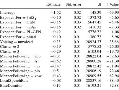
Compared to monomorphemic words ending with S, S duration was shorter when S realized plural, 3rdSg, GEN, and has/is. Plag et al. (Reference Plag, Homann and Kunter2017) observed a difference as well for genitive plurals, but for the full Buckeye, this contrast was not supported. Furthermore, as in the study of Plag et al. (Reference Plag, Homann and Kunter2017), the S was articulated with shorter duration when realizing has or is compared to when it realizes plurals or the third person singular. Plag et al. (Reference Plag, Homann and Kunter2017) observed an interaction of ExponentFor by Voicing, but this interaction did not replicate for the enlarged dataset. The differences between the present analysis and that of Plag et al. (Reference Plag, Homann and Kunter2017) have two possible sources. First, Plag et al. (Reference Plag, Homann and Kunter2017) manually inspected all data points and curated the automatic annotations and segmentations where necessary. By contrast, we followed the annotations and segmentations provided by the Buckeye corpus, which are also generally manually corrected on the basis of forced alignments. It is unclear at what level of carefulness the original manual corrections of the Buckeye corpus were performed. In addition, whereas misalignment tends to be very consistent and systematic in forced aligners, human annotators can be biased by their own expectations and create different kinds of variations in the annotation (Ernestus & Baayen Reference Ernestus and Harald Baayen2011). Therefore, there is no way to know which annotation can be strongly relied on, especially for phones with gradual transitions such as sonorants. Second, by considering the full corpus, the present analysis is possibly somewhat more robust against spurious small-sample effects. For instance, in the dataset of Plag et al. (Reference Plag, Homann and Kunter2017), there were only 81 voiced S tokens, as opposed to 563 voiceless S tokens. Table 3 summarizes a comparison of the significant contrasts for unvoiced S in the small sample of Plag et al. (Reference Plag, Homann and Kunter2017) with those found in the full corpus used here. Apart from one contrast, all contrasts are significant in both datasets.
Table 3 Significant contrasts for unvoiced S in the small sample of Plag et al. (Reference Plag, Homann and Kunter2017) and the present replication study (see Table 2). ‘Yes’ indicates an effect found in both studies and ‘no’ indicates an effect found only in the small sample, for  $\unicode[STIX]{x1D6FC}=0.05$ (under Tukey’s HSD) (s = non-morphemic final S, 3rdSg = 3rd person singular, GEN = genitive, PL-GEN = plural genitive).

Two things are important to note. First, the main finding of Plag et al. (Reference Plag, Homann and Kunter2017) is the difference in duration between unvoiced non-morphemic S (longest), clitic S, and suffix S (shortest). This difference is also found in the larger dataset with automatic annotation. Second, while in the Plag et al. (Reference Plag, Homann and Kunter2017) data set there was a significant interaction between voicing and morpheme type, this interaction is no longer present in the larger dataset.
To summarize, we have replicated the main findings of Plag et al. (Reference Plag, Homann and Kunter2017) for a much larger dataset derived from the same speech corpus. However, we still lack an explanation for the durational patterns observed. In the following sections, we will provide such an explanation, arguing that durational variation in word-final S is chiefly influenced by how strongly the final S is associated with its morphological function as a result of learning. This association strength will be derived from a naïve discriminative learning network, as explained in the next section.
4 Naïve discriminative learning
4.1 General overview
Naïve discriminative learning (NDL) is a computational modeling framework that is grounded in simple but powerful principles of discrimination learning (Ramscar & Yarlett Reference Ramscar and Yarlett2007, Ramscar et al. Reference Ramscar, Yarlett, Dye, Denny and Thorpe2010, Baayen et al. Reference Baayen, Milin, Filipović Durdević, Hendrix and Marelli2011, Rescorla Reference Rescorla1988). The general cognitive mechanisms assumed in this theory have been shown to be able to model a number of important effects observed in animal learning and human learning, e.g. the blocking effect (Kamin Reference Kamin, Campbell and Church1969) and the feature-label ordering effect (Ramscar et al. Reference Ramscar, Yarlett, Dye, Denny and Thorpe2010). NDL has recently been extended to language learning and language usage, and several studies have shown that it can successfully model different morphological phenomena and their effects onto human behavior, e.g. reaction times in experiments investigating morphological processing (e.g. Baayen et al. Reference Baayen, Milin, Filipović Durdević, Hendrix and Marelli2011, Blevins, Ackerman & Malouf Reference Blevins, Ackerman, Malouf, Harley and Siddiqi2016; see Plag Reference Plag2018: Section 2.7.7 for an introduction).
Discriminative learning theory rests on the central assumption that learning results from exposure to informative relations among events in the environment. Humans (and other organisms) use these relations, or ‘associations’, to build cognitive representations of their environments. Crucially, these associations (and the resulting representations) are constantly updated on the basis of new experiences. Formally speaking, the associations are built between features (henceforth cues) and classes or categories (henceforth outcomes) that co-occur in events in which the learner is predicting the outcomes from the cues. The association between cues and outcomes is computed mathematically using the so-called Rescorla–Wagner equations (Rescorla & Wagner Reference Rescorla, Wagner, Black and Prokasy1972, Wagner & Rescorla Reference Wagner, Rescorla, Boakes and Halliday1972, Rescorla Reference Rescorla1988; see Appendix A for a technical description). The equations work in such a way that the association strength or ‘weight’ of an association between a cue and an outcome increases every time that this cue and outcome co-occur. Importantly, this association weight decreases whenever the cue occurs without the outcome being present in a learning event. During learning, weights are continuously recalibrated. At any stage of learning, the association weight between a cue and an outcome can be conceptualized as the support which that specific cue can provide for that specific outcome given the other cues and outcomes which had been encountered during the learning history.
Let us look at an example of how our understanding of the world is constantly modulated by the matches and mismatches between our past experiences and what we actually observe. Our example is a phenomenon known as ‘anti-priming’ found by Marsolek (Reference Marsolek2008). He presented speakers with sequences of two pictures and asked these speakers to say the name of the second picture. The critical manipulation was implemented in the first picture, which could be either similar, to some extent, to the target picture (e.g. grand piano, followed by table), or unrelated (e.g. orange, followed by table). In contrast to typical priming findings, Marsolek observed that speakers responded more quickly for unrelated pairs compared to related pairs. This ‘anti-priming’ – caused by prior presentation of a related picture – follows straightforwardly from the learning rule of Rescorla & Wagner (Reference Rescorla, Wagner, Black and Prokasy1972). The weights of visual features (i.e. the cues) that are shared by grand piano and table, such as having legs and a large flat surface, are strengthened for grand piano but weakened for table when the picture of the grand piano is presented. Slower response times in this case of anti-priming are a direct consequence of critical features losing strength to table compared to cases in which a visually unrelated prime, such as an orange, had been presented.
Taking a morphological example, the association of the phonological string /aɪz/ with a causative meaning (‘make’) in English would be strengthened each time a listener encounters the word modernize and weakened each time the listener hears the words size or eyes. The association strengths resulting from such experiences influence language processing in both production and comprehension.
Technically, the mathematical engine of NDL, i.e. the Rescorla–Wagner equations, is an optimized computational implementation of an error-driven discrimination learning. This engine can be viewed as implementing ‘incremental regression’ (for a nearly identical algorithm from physics, see Widrow & Hoff (Reference Widrow and Hoff1960) and for a Bayesian optimized algorithm, Kalman (Reference Kalman1960)). NDL was first applied to large corpus data and used to study chronometric measures of lexical processing by Baayen et al. (Reference Baayen, Milin, Filipović Durdević, Hendrix and Marelli2011). An extension of the learning algorithm is reported in Sering, Milin & Baayen (Reference Sering, Milin and Baayen2018b). Implementations are available both for R (Shaoul et al. Reference Shaoul, Schilling, Bitschnau, Arppe, Hendrix and Baayen2014) and Python (Sering et al. Reference Sering, Weitz, Kuenstle and Schneider2018a).
Once a network has been trained, it provides different measures that represent different aspects of the association strength between cues and outcomes. These measures may subsequently be used as predictors of human responses (e.g. response times in lexical decision experiments). In the present study, we will use three NDL measures to predict the acoustic duration of S in regression analyses.
Other approaches to learning are available, for instance, the Bayesian model presented in Kleinschmidt & Jaeger (Reference Kleinschmidt and Jaeger2015). Where NDL comes into its own, compared to models based on probability theory, is when there are thousands or tens of thousands of different features (cues) that have to be learned to discriminate equally large numbers of classes (outcomes). Cues compete for outcomes in often unforeseeable ways reminiscent of chaotic systems, which is why it is a truly daunting challenge to capture the dynamics of such systems with probabilities defined over hand-crafted hierarchies of units (i.e. with probabilistic statistics). Errors at lower levels of the hierarchy tend to propagate to higher levels and render the performance of such models less than optimal. This is why in computational linguistics, there is a strong movement in the direction of end-to-end models which bypass the engineering by hand of intermediate representations using neural networks. NDL adopts this end-to-end approach. In contrast to approaches in machine learning, however, NDL does not use any hidden layers. Rather, it makes use of the simplest possible network architecture, with just one input layer and one output layer.
NDL thus offers a simple method for assessing the consequences of discrimination learning that has hardly any free parameters (namely, only a learning rate, typically set to 0.001, and the maximum amount of learning  $\unicode[STIX]{x1D706}$, set to 1.0). Consequently, once the representations for the input and output layers of the network have been defined and the learning rate and $\unicode[STIX]{x1D706}$ have been set, its performance is determined completely by the corpus on which it is trained.
NDL also differs from standard applications of neural networks in machine learning in that it uses very large numbers of input and output features. We therefore refer to the NDL networks as ‘wide learning’ networks. The weights of these networks are updated incrementally by applying the learning rule of Rescorla and Wagner to the so-called learning events. Learning events are defined as moments in learning time at which a set of cues and a set of outcomes are evaluated jointly. Association weights between cues and outcomes are strengthened for those outcomes that were correctly predicted and weakened for all other outcomes. For technical details, see Milin et al. (Reference Milin, Feldman, Ramscar, Hendrix and Baayen2017b) and Sering et al. (Reference Sering, Milin and Baayen2018b), and for a simple introductory implementation, see Plag (Reference Plag2018: Section 7.4.4).
This approach to simulate language learning has proved useful for, e.g. modeling child language acquisition (Ramscar et al. Reference Ramscar, Yarlett, Dye, Denny and Thorpe2010, Reference Ramscar, Dye, Popick and O’Donnell-McCarthy2011, Ramscar, Dye & Klein Reference Ramscar, Dye and Klein2013a, Ramscar et al. Reference Ramscar, Dye and McCauley2013b), for disentangling linguistic maturation from cognitive decline over the lifespan (Ramscar et al. Reference Ramscar, Hendrix, Shaoul, Milin and Baayen2014, Reference Ramscar, Sun, Hendrix and Baayen2017), for predicting reaction times in the visual lexical decision task (Baayen et al. Reference Baayen, Milin, Filipović Durdević, Hendrix and Marelli2011, Milin et al. Reference Milin, Feldman, Ramscar, Hendrix and Baayen2017b) and self-paced reading (Milin, Divjak & Baayen Reference Milin, Divjak and Baayen2017a), as well as for auditory comprehension (Baayen et al. Reference Baayen, Shaoul, Willits and Ramscar2016b, Arnold et al. Reference Arnold, Tomaschek, Lopez, Sering and Baayen2017). The computational model developed by Arnold et al. (Reference Arnold, Tomaschek, Lopez, Sering and Baayen2017) is based on a wide learning network that has features derived automatically from the speech signal as input. This model outperformed off-the-shelf deep learning models on single-word recognition and shows hardly any degradation in performance when presented with speech in noise (see also Shafaei Bajestan & Baayen Reference Shafaei Bajestan and Baayen2018).
By adopting an end-to-end approach with wide learning, naïve discriminative learning approaches morphology, the study of words’ forms and meanings, from a very different perspective than the standard post-Bloomfieldian hierarchical calculus based on phonemes, morphemes, and words. The relation between form and meaning is addressed directly, without intervening layers of representations. In what follows, we will make use of wide learning networks primarily as a convenient tool from machine learning. In Section 6, we will briefly return to the question of the implications of successful end-to-end learning for morphological theory.
4.2 From NDL to phonetic durations
The present study follows up on Tucker et al. (Reference Tucker, Sims and Baayen2019), who used NDL measures to predict the durations of stem vowels of regular and irregular verbs in English in the Buckeye corpus. Their NDL wide learning network had diphones as cues, and as outcomes both content lexemes (or more specifically, pointers to the meanings of content words) and morphological functions (such as plural or the clitic has). In what follows, we refer to these pointers to meanings/functions as lexomes (see Milin et al. Reference Milin, Feldman, Ramscar, Hendrix and Baayen2017b for a detailed discussion). Tucker et al. observed that the prediction accuracy of statistical model fits to vowel duration improved substantially when classical predictors such as frequency of occurrence and neighborhood density were replaced by predictors grounded in naïve discriminative learning.
Following their lead, we implemented a network that has morphological function lexomes as outcomes, but restricted them to those that are implicated with English word-final S: clitic, genitive plural, genitive singular, plural noun, singular noun, third person verb, verb, verb participle, past-tense verb, and other (such as adverbs). The number of morphological functions is larger than that examined in the original Plag et al. (Reference Plag, Homann and Kunter2017) study, as we also include S that is word-final in past-tense or past-participle forms as a result of reduction (e.g. in pass for passed). Voicing of S was based on the phonetic transcription provided by the Buckeye corpus.
The findings by Tucker et al. (Reference Tucker, Sims and Baayen2019) indicate that speakers have to balance opposing forces during articulation, one that seeks to lengthen parts of the signal in the presence of strong bottom-up support and one that seeks to shorten them in case of high uncertainty. To parameterize these forces, we derived three different measures from the NDL wide learning network which are used as predictors of S duration: the S lexomes’ activations, their priors, and their activation diversities. Table 4 provides an example of a simple NDL network where the diphone cues for the word form ‘dogs’ are associated with, among others, the lexome of the morphological function plural. We will discuss each measure in turn.
Table 4 The table illustrates a cue-to-outcome network with a set of cues  ${\mathcal{C}}$ with $k$ cues $c$ and a set of lexome outcomes ${\mathcal{O}}$ with $n$ outcomes $o$. We illustrate the calculation of NDL measures for the lexome of the morphological function plural as an outcome, located in the second column, and its associated cue set ${\mathcal{C}}_{\unicode[STIX]{x1D6FA}}=\mathtt{ld~dO~Og~gz~zb}$, located in rows 3–7. Each $i\mathit{th}$ cue $c$ is associated with each $j\mathit{th}$ outcome $o$ by a weight $w_{i,j}$, representing their connection strength, where $i=1,2,\ldots ,k$ and $j=1,2,\ldots ,n$. Summed weights for ${\mathcal{C}}_{\unicode[STIX]{x1D6FA}}$ afferent to $o_{j}$ give the $j\mathit{th}$ activation $a$. The cues in $c_{1}$, $c_{2}$ represent any kind of cues that might occur in the first and second row.

A lexome’s activation represents the bottom-up support for that lexome, given the cues in the input. The activation for a given lexome is obtained simply by the summation of the weights on the connections from those cues that are instantiated in the input to that outcome (equivalent to the weights marked in red in Table 4). Hence, activation represents a measure of the cumulative evidence in the input.
A lexome’s prior is a measure of an outcome’s baseline activation, calculated by the sum of all absolute weights pertinent to the lexome outcome (equivalent to the weights in the column marked in light gray in Table 4).Footnote [5] The prior can be understood as a measure of network entrenchment. It is an NDL measure that is independent of a particular input to the network; rather it captures a priori availability which results from learning and typically corresponds to frequency of occurrence.
Finally, a lexome’s activation diversity is a measure of the extent to which the input makes contact with the lexicon. Activation diversity is the sum of the absolute activations pertinent from a cue set to all lexome outcomes (equivalent to the activations located in the bottom row highlighted in dark gray in Table 4). One can think of this measure as quantifying the extent to which the cues in the input perturb the state of the lexicon. If the cues were to support only the targeted outcome, leaving all other outcomes completely unaffected, then the perturbation of the lexicon would be relatively small. However, in reality, learning is seldom this crisp and clear-cut, and the states of outcomes other than the targeted ones are almost always affected as well. In summary, the more the lexicon as a whole is perturbed, the greater the uncertainty about the targeted lexomes will be.
Tucker et al. (Reference Tucker, Sims and Baayen2019) observed that vowel duration decreased with activation diversity. When uncertainty about the targeted outcome increases, acoustic durations decrease (for further examples of shortening under uncertainty, see also Kuperman et al. (Reference Kuperman, Pluymaekers, Ernestus and Baayen2007) and Cohen (Reference Cohen2014a)). Arnold et al. (Reference Arnold, Tomaschek, Lopez, Sering and Baayen2017) performed an auditory experiment in which subjects had to indicate whether they could identify the words presented to them. These words were randomly selected from the GECO corpus (Schweitzer & Lewandowski Reference Schweitzer and Lewandowski2013). Arnold et al. observed that words with low activation diversity (i.e. with short vectors that hardly penetrate lexical space) were quickly rejected, whereas words with large activation diversity (i.e. with long vectors that reach deep into lexical space) were more likely to be identified, but at the cost of longer response times.
Tucker et al. (Reference Tucker, Sims and Baayen2019) also observed that prediction accuracy decreases when instead of using the diphones in the transcription of what speakers actually said, the diphones in the dictionary forms are used. We therefore worked with diphones derived from the actual speech. However, we considered a broader range of features as cues.
Several studies that made use of discriminative learning actually worked with two networks, one network predicting lexomes from form cues, resulting in form-to-lexome networks, and the other predicting lexome outcomes from lexome cues, creating lexome-to-lexome networks (Baayen et al. Reference Baayen, Shaoul, Willits and Ramscar2016b, Milin et al. Reference Milin, Divjak and Baayen2017a, Reference Milin, Feldman, Ramscar, Hendrix and Baayenb, Baayen, Milin & Ramscar Reference Baayen, Milin and Ramscar2016a). Lexome-to-lexome networks stand in the tradition of distributional semantics (Landauer & Dumais Reference Landauer and Dumais1997, Lund & Burgess Reference Lund and Burgess1996a, Shaoul & Westbury Reference Shaoul and Westbury2010a, Mikolov et al. Reference Mikolov, Sutskever, Chen, Corrado, Dean, Burges, Bottou, Welling, Ghahramani and Weinberger2013). The row vectors of the weight matrix of lexome-to-lexome networks of NDL specify, for each lexome, the association strengths of that lexome with the full set of lexomes. These association strengths can be interpreted as gauging collocational strengths. In the present study, we do not work with a separate lexome-to-lexome network. Rather, we used a joint network that contains both lexomes and their diphones as cues and morphological functions as outcomes.Footnote [6]
4.3 Cue-to-outcome structure
Let us now turn to the actual modeling procedures that we employed and the evaluation of these models that led us to focus on inflectional lexomes as outcomes.
As a general strategy, we wanted to explore various constellations of cues and outcomes. We also considered the possibility that S duration might be co-determined by the lexomes in a word’s immediate context. Therefore, just as in models for distributional semantics, such as those presented by Lund & Burgess (Reference Lund and Burgess1996b), Shaoul & Westbury (Reference Shaoul and Westbury2010b), and Mikolov et al. (Reference Mikolov, Sutskever, Chen, Corrado, Dean, Burges, Bottou, Welling, Ghahramani and Weinberger2013), we placed an n-word window around a given target word and restricted cues and outcomes to features within this window. By varying the window size between zero and maximally two to the left or the right of the target word, and the specific features selected for cues and outcomes, we obtained a total of 38 NDL networks.
We created diphone cues on the basis of an entire phrase. This procedure created transition cues between words. A sequence such as ‘dogs bark’ gives the diphone cues dO Og gz zb bA Ar rk with zb as the transition cue.
Table 5 illustrates several different choices for cues and outcomes, given the phrase the small dogs bark at the cat, where dogs is the pivotal word carrying S. Examples 1, 2, and 5 illustrate models in which lexomes are outcomes and examples 3 and 4 have diphones as outcomes. Example 1 has only diphones as cues, and this model is a standard form-to-lexome network following the approach originally taken by Baayen et al. (Reference Baayen, Milin, Filipović Durdević, Hendrix and Marelli2011) and Tucker et al. (Reference Tucker, Sims and Baayen2019). Example 2 has lexomes as cues and outcomes; this is a standard lexome-to-lexome network (see Baayen et al. Reference Baayen, Milin and Ramscar2016a, Milin et al. Reference Milin, Feldman, Ramscar, Hendrix and Baayen2017b for applications of such networks for modeling reaction times). Model 3 seeks to predict diphones from lexomes. Model 4 complements the lexome cues with diphone cues. Model 5 also combines lexomes and diphones as cues, but these are used to predict lexomic outcomes. Importantly, these lexomes include the inflectional lexomes that are realized with S in English. The pertinent lexome in the present example is the one for plural number (plural). Note that model 5 allows us to test the hypothesis that the support for plural is obtained not only from a word’s diphones but also from its collocates.
Table 5 Possible cue–outcome configurations for the phrase the small dogs bark at the cat using a five-word window centered on dogs.

Models were trained by moving a given word window across the whole of the Buckeye corpus.Footnote [7] The window was moved across the corpus such that each word token was in the center of the window once. Consequently, a given S word will have occurred in each of the positions in the window. Each window provided a learning event at which prediction accuracy was evaluated and connection weights were recalibrated.
A wide variety of selections of cues and outcomes was investigated with the aim of obtaining insight into which combinations of cues and outcomes, under a discriminative learning regime, best predict S duration. Models with lexomes as outcomes, specifically those for the morphological functions of the S (clitic, genitive plural, genitive singular, plural noun, singular noun, third person verb, verb, verb participle, past-tense verb, and other) address the possibility that it is the learnability of the inflectional lexomes that drives the acoustic duration of S. Models that take diphones as outcomes address the hypothesis that it is the learnability of diphones (i.e. of context-sensitive phones) that is at issue.
In classical models of speech production, e.g. the weaver model of Levelt et al. (Reference Levelt, Roelofs and Meyer1999) and the model of Dell (Reference Dell1986), the flow of processing goes from conceptualization to articulation. Against this background, models in which lexomes are predicted instead of being predictors are unexpected. Nevertheless, there are three reasons why it makes sense to include such models in our survey.
First, for a survey, it is important to consider a wide range of possible combinations, including ones that are at first sight counter-intuitive. This is essential for allowing data to inform theory.
The second reason is technical in nature: NDL makes the simplifying assumption that each outcome can be modeled independently from all other outcomes. It is this assumption that motivates why NDL is referred to as naïve discriminative learning. For discriminative learning to take place, multiple cues are required for a given outcome so that over learning time it can become clear, due to cue competition, which cues are informative and which are uninformative. Informative cues obtain larger association strengths and uninformative cues obtain association strengths close to zero. If the learnability of inflectional lexomes is what drives S duration, then the NDL network must include inflectional lexomes as outcomes. If we were to take these inflectional lexomes as cues and use them to predict a diphone such as gz as outcome, the network would only learn the relative frequencies with which the inflectional lexomes are paired with gz in the corpus (cf. Ramscar et al. Reference Ramscar, Yarlett, Dye, Denny and Thorpe2010).
Third, any production system must have some form of feedback control so that the sensory consequences of speaking can be evaluated properly. Without such feedback, which comprises sensory feedback from the articulators as well as proprioceptive feedback from hearing one’s own speech, learning cannot take place (see Hickok Reference Hickok2014 for a detailed discussion). For the error-driven learning to be at all possible, distinct articulatory and acoustic targets must be set up before articulation, against which the feedback from the articulatory and auditory systems can be compared. In what follows, the diphone outcomes are a crude approximation of the speaker’s acoustic targets, and the connections from the diphones to the lexomes are part of the speech control loop. For a computational model providing a more detailed proposal for resonance between the production and comprehension systems, see Baayen et al. (Reference Baayen, Chuang, Shafaei-Bajestan and Blevins2019).
4.4 NDL measures as predictors
Having trained the 38 networks, we then analyzed their performance using random forests (as implemented in the party package for R), focusing on the variable importance of the NDL measures derived from these networks. The optimal network that emerged from this analysis is the one with a five-word window and the structure of example 5 in Table 5. Critical lexomes, i.e. morphological functions, were predicted from all lexomes and their diphones within a five-word window centered on the target word. Given the literature on conditional probabilities for upcoming (or preceding) information, such as the probability of the current word, given the next word (Jurafsky et al. Reference Jurafsky, Bell, Girand and Gussenhoven2000, Pluymaekers et al. Reference Pluymaekers, Ernestus and Baayen2005b, Tremblay et al. Reference Tremblay, Derwing, Libben and Westbury2011, Bell et al. Reference Bell, Brenier, Gregory, Girand and Jurafsky2009), we included in our survey of cue and outcome structures windows of size three, with the target word in either first or second position. The corresponding networks lacked precision compared to the above network trained on learning events of five words.Footnote [8] The latter network is also sensitive to co-occurrence of the target word with the preceding and upcoming word, but it is sensitive as well to co-occurrence with words further back and further ahead in time.
In the light of the literature on boundary strength and its consequences for lexical processing (Seidenberg Reference Seidenberg and Coltheart1987, Weingarten, Weingarten & Will Reference Weingarten, Nottbusch, Will, Pechmann and Habel2004, Hay Reference Hay2002, Reference Hay2003, Hay & Baayen Reference Hay, Baayen, Booij and Van Marle2002, Baayen et al. Reference Baayen, Shaoul, Willits and Ramscar2016b, Reference Baayen, Chuang, Shafaei-Bajestan and Blevins2019), we considered separately the activation and activation diversity calculated for the diphone straddling the boundary between stem and S, and the activation and activation diversity calculated from all other remaining cues (lexomes and diphones). This resulted in a total of five NDL measures as predictors of S duration:
1. PriorMorph: the prior for weights from a cue set to a word’s inflectional lexome.
2. ActFromBoundaryDiphone: the activation of an inflectional lexome by the boundary diphone.
3. ActFromRemainingCues: the activation of an inflectional lexome by all other (lexome and diphone) cues.
4. ActDivFromBoundaryDiphone: the activation diversity calculated over the vector of activations over all inflectional lexomes of S, given the boundary diphone as cue.
5. ActDivFromRemainingCues: the activation diversity, again calculated over the vector of activations of all inflectional lexomes, but now using the remaining cues in the learning event.
There are nine values that PriorMorph can assume, one value for each of the nine inflectional lexomes that we distinguished (clitic, genitive plural, genitive singular, plural noun, singular noun, third person verb, verb, verb participle, past-tense verb, and other). The boundary diphone will usually differ from word to word depending on the stem-final consonant and the specific realization of the S. For any specific boundary diphone, there are again nine possible values of ActFromBoundaryDiphone and ActDivFromBoundaryDiphone, one for each inflectional lexome. For a given target word, e.g. dogs, we consider the activation and activation diversity, given [gz] as cue, for the corresponding inflectional outcome, here noun plural. The values of ActFromRemainingCues and ActDivFromRemainingCues depend on the words that happen to be in the moving window, and hence their values vary from token to token. In this way, each target word was associated with five measures for its inflectional lexome.
Although the prior, activation, and activation diversity measures have been found to be useful across many studies, there is considerable uncertainty about how they might predict the duration of English S.
With respect to PriorMorph, the general strong correlation of NDL priors with word frequency would suggest, given the many studies reporting durational shortening for increasing frequency (see, e.g. Zipf Reference Zipf1929, Jurafsky et al. Reference Jurafsky, Bell, Gregory, Raymond, Bybee and Hopper2001a, Bell et al. Reference Bell, Jurafsky, Fosler-Lussier, Girand, Gregory and Gildea2003, Gahl Reference Gahl2008), that a greater PriorMorph correlates with shorter S. However, recent findings emerging from production studies using electromagnetic articulography suggest that a higher prior (or frequency of occurrence) might predict increased rather than decreased S duration: Tomaschek et al. (Reference Tomaschek, Tucker, Baayen and Fasiolo2018c) observed that, other things being equal, greater frequency enables speakers to execute articulatory gestures with more finesse, in parallel to the general finding that motor skills improve with practice. It is also possible that PriorMorph will not be predictive at all, as Tucker et al. (Reference Tucker, Sims and Baayen2019) did not observe an effect of the prior for stem vowel duration.
For the activation measures (ActFromBoundaryDiphone and ActFromRemainingCues), our expectation is that a greater activation will afford durational lengthening. Arnold et al. (Reference Arnold, Tomaschek, Lopez, Sering and Baayen2017) observed, using an auditory word identification task, that a greater activation corresponded to higher recognition scores. Since a higher signal to noise ratio is expected to give rise to improved recognition rates, the prediction follows for English S that when the activation is higher, there must be more signal compared to noise, and this higher signal to noise ratio is, for a fricative such as S, likely to be realized by lengthening. This is indeed what Tucker et al. (Reference Tucker, Sims and Baayen2019) observed for vowel duration in regular verbs: as activation increased, the duration of the stem vowel increased likewise.
Turning to the activation diversity measure, here Tucker et al. (Reference Tucker, Sims and Baayen2019) observed a strong effect, with larger activation diversity predicting shorter duration. This result fits well with the finding of Arnold et al. (Reference Arnold, Tomaschek, Lopez, Sering and Baayen2017) that in auditory word identification, words with a low activation diversity elicited fast negative responses, whereas words with higher activation diversity had higher recognition scores that came with longer decision times. In fact, the activation diversity measure can be understood as a measure of lexicality: a low lexicality is an index of noise, whereas a high lexicality indicates that the speech signal is making contact with possibly many different words. The other side of the same coin is that discriminating the target lexome in a densely populated subspace of the lexicon takes more time. For speech production, Tucker et al. (Reference Tucker, Sims and Baayen2019) argued that when lexicality is high, the system is in a state of greater uncertainty as many lexomes are co-activated with the targeted outcome. Importantly, if some part of the signal, e.g. English S, contributes to greater uncertainty, it is disadvantageous for both the listener and the speaker to extend its duration. All that extending its duration accomplishes is that uncertainty is maintained for a longer period of time. It makes more sense to reduce the duration of those parts of the signal that do not contribute to discriminating the targeted outcome from its competitors. These considerations led us to expect a negative correlation between activation diversity and S duration.
5 Results
We analyzed the log-transformed duration of S with a generalized additive mixed model (GAMM, Wood Reference Wood2006, Reference Wood2011) with random intercepts for the speaker and the word. In addition to the five measures derived from the NDL network, we controlled for the manner of the preceding and following segment by means of two factors, one for the preceding segment and one for the following segment (each with levels approximant, fricative, nasal, plosive, vowel, and absent). We included the average speaking rate of the speaker (IndividualSpeakingRate) and the local speaking rate (LocalSpeakingRate) as control covariates.
In a number of cases, the S-bearing word would be located in a phrase final position and the last diphone cue would be s# or z#. These cues resulted in strong outliers in the NDL measures, which is why these words were excluded from analysis. A total of 27091 tokens was investigated with NDL measures; Table 6 shows the number of tokens depending on function and voicing.
Table 6 Number of S tokens in each morphological function split by voicing investigated with NDL measures.

The model we report here is the result of exploratory data analysis in which the initial model included all control predictors and the random effect factors but no NDL measures. We then added in NDL measures step by step, testing for non-linearities and interactions. Model criticism of the resulting generalized additive mixed model (GAMM) revealed that the residuals deviated from normality. This was corrected for by refitting the model with a GAMM that assumes that the scaled residuals follow a  $t$-distribution (Wood, Pya & Säfken Reference Wood, Pya and Säfken2016). The scaled $t$-distribution adds two further parameters to the model, a scaling parameter $\unicode[STIX]{x1D70E}$ (estimated at 6.18) and a parameter for the degrees of freedom $\unicode[STIX]{x1D708}$ of the $t$-distribution (estimated at 0.29). Thus, for the present data, the residual error is characterized by $\unicode[STIX]{x1D716}/6.18\sim t_{(0.29)}$. Table 7 and Figures 1–3 are based on this model.
Table 7 Summary of parametric and smooth terms in the generalized additive mixed model fit to the log-transformed acoustic duration of S as pronounced in the Buckeye corpus. The reference level for the preceding and following manner of articulation is ‘absent’.

As the present model is the result of exploratory data analysis, the  $p$-values in Table 7, which all provide strong support for model terms with NDL measures as predictors, cannot be interpreted as the long-run probability of false positives. One might apply a stringent Bonferroni correction, and we note here that the large $t$-values for NDL model terms easily survive a correction for 1000 or even 10000 tests. However, we prefer to interpret the $p$-values simply as a measure of surprise and an informal point measure of the relative degree of uncertainty about the parameter estimates.
Figure 1 presents the partial effect of PriorMorph. Larger priors go together with longer durations. This effect levels off slightly for larger priors. Apparently, inflectional lexomes with a stronger baseline activation tend to be articulated with longer durations. The 95% confidence interval (or more precisely, as GAMMs are empirical Bayes, the 95% credible interval) is narrow, especially for predictor values between 5 and 25, where most of the data points are concentrated.

Figure 1 Partial effect of PriorMorph in the GAMM fit to S duration, with 95% confidence (credible) interval.
Recall that PriorMorph has nine different values, one for each inflectional function of S. It is noteworthy that when we replace PriorMorph by a factor with the nine morphological functions as its levels, the model fit decreases (by 10 ML-score units), while at the same time the number of parameters increases by 7. The NDL prior for the inflectional functions, just by itself, already provides more precision for predicting the duration of English S. Further precision is gained by also considering the activation and activation diversity measures.
Figure 2 presents the partial effect of the interaction of ActFromBoundaryDiphone and ActDivFromBoundaryDiphone, which we modeled with a tensor product smooth. The left panel presents the contour lines with 1SE confidence intervals; the right panel shows the corresponding contour plot in color to facilitate interpretation, with darker shades of blue indicating shorter S and warmer yellow colors denoting longer S. The narrow confidence bands in the left panel indicate that there are real gradients in this regression surface, except for the upper left corner of the plotting region. For all activation values, we find that as the activation diversity increases, S duration decreases. Conversely, for most values of activation diversity, increasing the activation leads to larger S duration. Shortest S durations are found for larger (but not the largest) values of activation and for activation diversities exceeding 0.2. The two boundary measures interact insofar as S duration is strongly reduced for high DivLastDiphone in spite of high ActLastDiphone, as can be seen by the lake-like blue dip in the upper right quadrant of the plot. While smaller activation – and consequently reduced support – for the morphological function of S should result in shorter S, it seems as though greater certainty about the morphological function counterbalances the trend, resulting in longer S (bottom left quadrant of the plot).

Figure 2 Partial effect in the GAMM fit to log-transformed S duration of the activation and activation diversity of the boundary diphone. In the right plot, deeper shades of blue indicate shorter acoustic durations and warmer shades of yellow denote longer durations. The left plot presents contour lines with 1SE confidence bands.
Figure 3 visualizes the three-way interaction of ActFromRemainingCues by ActDivFromRemainingCues by local speaking rate.Footnote [9] The successive panels of Figure 3 present the odd deciles of local speaking rate (0.1, 0.3, 0.5, 0.7, and 0.9). The regression surface slowly morphs from one with long durations for high ActDivFromRemainingCues (left panel) to a surface with long durations only in the lower right corner. The general pattern for ActDivFromRemainingCues is that S duration decreases as ActDivFromRemainingCues increases. For the lowest two deciles of local speech rate, this effect is absent for high values of ActFromRemainingCues. For ActFromRemainingCues, we find that for lower values of ActDivFromRemainingCues, durations increase with activation. For higher activation diversities, this effect is U-shaped. The interaction pattern between the two NDL measures mirrors the one found in Figure 2.

Figure 3 Tensor product smooth for the three-way interaction of ActFromRemainingCues by ActDivFromRemainingCues by local speaking rate. The regression surface for the two activation measures is shown for deciles 0.1, 0.3, 0.5, 0.7, and 0.9 of local speaking rate. Deeper shades of blue indicate shorter acoustic durations and warmer shades of yellow denote longer durations.
6 Discussion
6.1 Summary of the present results
Plag et al. (Reference Plag, Homann and Kunter2017) reported that there are significant differences in the duration of English S as a function of the inflectional function realized by this exponent (see also Zimmermann Reference Zimmermann, Carignan and Tyler2016a, Seyfarth et al. Reference Seyfarth, Garellek, Gillingham, Ackerman and Malouf2018). Plag et al. (Reference Plag, Homann and Kunter2017) observed that these differences in acoustic duration challenge the dominant current theories of morphology. These theories, which have their roots in post-Bloomfieldian American structuralism, hold that the relation between form and meaning in complex words is best understood in terms of a calculus in which rules operate on bound and free morphemes as well as on phonological units such as syllables and feet. However, the units of this theory, the configurations of these units, or the rules operating on these units or ensembles thereof cannot explain the observed differences in the duration of English S in an insightful way.
The present study explored whether the different durations of S can be understood as following from the extent to which words’ phonological and collocational properties can discriminate between the inflectional functions expressed by the S. We quantified the discriminability of these inflectional functions with three measures derived from a wide learning discrimination network that was trained on the entire Buckeye corpus. The input features (cues) for this network were words’ lexomes in a five-word window centered on the S-bearing word and the diphones in the phonological forms of these lexomes. The classes to be predicted from these cues (the outcomes) were the inflectional functions (inflectional lexomes) of the S.
Three measures derived from the network were predictive for the duration of S. A greater activation of a word’s inflectional lexome (i.e. greater bottom-up support) predicted longer durations. A higher lexomic prior (i.e. a higher baseline activation or, equivalently, a higher degree of entrenchment in the network) also predicted longer durations. Apparently, both the support for a word’s morphological function that is provided by that word’s form and its collocational patterning as well as the a priori baseline support for the word that accumulates over the course of learning give rise to a prolonged acoustic signal. In other words, stronger support, both long-term and short-term, for a morphological function leads to an enhanced signal.
This finding dovetails well with lengthening of interfixes in Dutch, enhancement of English suffixes when they are paradigmatically more probable, and enhancement of vowels in Russian in proportion to paradigmatic support (Kuperman et al. Reference Kuperman, Pluymaekers, Ernestus and Baayen2007, Cohen Reference Cohen2014a, Reference Cohenb, Reference Cohen2015). Signal enhancement as a function of activation also replicates the findings of Tucker et al. (Reference Tucker, Sims and Baayen2019) for the stem vowel of regular verbs in the Buckeye corpus.
The study by Tucker et al. (Reference Tucker, Sims and Baayen2019) reported an opposing force on the duration of verbs’ stem vowels: the activation diversity. Activation diversity is a measure of lexicality. It assumes high values when the cues in the input are linked to many different outcomes. In such a case, the outcome is located in a dense lexico-semantic subspace and it is more difficult to discriminate the targeted outcome from its competitors. For auditory comprehension, we thus find that processing is slowed when activation diversity is high (Arnold et al. Reference Arnold, Tomaschek, Lopez, Sering and Baayen2017). The flip side of the same coin is that in speech production, the prolonging part of the acoustic signal, such as S, is dysfunctional when this signal increases the discrimination problem. A signal that is not discriminable cannot be made more discriminable by prolonging it. The prolongation will result only in lengthening a state of uncertainty instead of contributing to resolving it. Importantly, a large activation diversity is dysfunctional not only for the listener but also for the speaker. The auditory image that the speaker projects and aims to realize through articulation (Hickok Reference Hickok2014) feeds back through the control loop to the semantic system. As a consequence, aspects of the speech signal that are problematic for the listener will also be problematic for the speaker.
Considered together, the three NDL measures indicate that the speaker has to balance two opposing forces. One force seeks to lengthen parts of the signal in the presence of strong bottom-up support and long-term expectations. The other force seeks to shorten parts of the signal that increase uncertainty. The NDL measures enable us to probe these forces. More importantly, our model illustrates that these two forces interact in an unexpected way. In case one force creates extreme uncertainty about the morphological function of S, the other force is able to reduce this uncertainty and S durations turn out to be long.
The framework of naïve discriminative learning accepts that the language system is, to some degree, ‘chaotic’. Just as in weather systems, a butterfly flapping its wings in the Amazon is claimed to be able to start a chain of events that cause a rainstorm in London (Lorenz Reference Lorenz1972), the cues that co-occur across learning events with cues that go together with a target word can co-determine the discriminability of that target word; see Mulder et al. (Reference Mulder, Dijkstra, Schreuder and Baayen2014) for an interpretation of the secondary family size effect along these lines.
Thus, the approach presented in the current study – training of an NDL network that learns to discriminate linguistic outcomes on the basis of sublexical and collocational properties and deriving NDL measures from this network to predict the acoustic properties of a linguistic item – can be adopted to investigate similar phenomena in other languages. For example, we are currently investigating how the different inflectional and derivational functions of final /s/ and final schwa in Dutch affect their acoustic durations. The approach allows one to investigate the lexical structure of not only morphological functions but maybe even semantic contrasts. Given the present results as well as those by Tucker et al. (Reference Tucker, Sims and Baayen2019), this approach is very promising.
6.2 Consequences for morphological theory
The question remains as to whether this ‘chaotic’ explanation of non-random variation in S duration improves on an explanation that simply posits that different morphological functions have different consequences for S duration. Rephrased statistically, does the prediction accuracy increase when we replace a model with a factor for morphological function (with nine levels) with a model in which this factor is replaced with NDL measures? When we replace the factor inflection type by just the NDL prior, a numeric variable with nine distinct values, model fit indeed improves, while at the same time model complexity decreases. Instead of needing eight parameters for inflectional function, only a single parameter (the slope of the regression line) suffices. When the linearity assumption for the prior is relaxed, the required effective degrees of freedom is still well below 8.
What are the consequences of our findings for morphological theory and theories of speech production? First, consider morphological theory. Here, we are confronted with a range of different approaches that rest on very different assumptions about the structure of words. Two major approaches are relevant in the context of the S problem. On the one hand, we have post-Bloomfieldian item-and-arrangement theories (IAA; Hockett Reference Hockett1954) and generative offshoots thereof building on Chomsky & Halle (Reference Chomsky and Halle1968). On the other hand, we have realizational theories such as word and paradigm morphology (WP) (Blevins Reference Blevins2006). Both WP and IAA address how inflectional functions such as number and tense are expressed in speech. IAA posits that this expression is mediated by morphemes, i.e. the minimal units of a language that combine form and meaning. WP, on the other hand, rejects the usefulness of the morpheme as a theoretical construct (see also Matthews Reference Matthews1974, Beard Reference Beard1977, Aronoff Reference Aronoff1994, Blevins Reference Blevins2003). Instead of constructing a calculus for building words out of morphemes, WP focuses on the paradigmatic relations between words and holds that morphological systematicities are driven by certain paradigm-internal mechanisms, e.g. proportional analogy. Naïve discriminative learning provides a computational modeling framework that is deeply influenced by WP morphology, and the measures derived from the model can be understood as gauging aspects of proportional analogies. The specific implementation proposed in this study of English S extends proportional analogy by including ‘collocational analogy’ along with phonological analogy. For a detailed discussion of proportional analogy and discriminative learning, see Baayen et al. (Reference Baayen, Chuang, Shafaei-Bajestan and Blevins2019).
It is less clear whether the present findings are compatible with IAA. Explanations within IAA can attribute an effect to representations for units, to configurations of such units, as well as to the combinatorial rules that give rise to these configurations. Plag et al. (Reference Plag, Homann and Kunter2017) showed that the observed differences in the durations of English S cannot be explained in this way. However, IAA can assign conditional probabilities to units and configurations of units and link the likelihood of an effect to such probabilities (see, among others, Jurafsky et al. Reference Jurafsky, Bell, Girand and Gussenhoven2000, Aylett & Turk Reference Aylett and Turk2004, Gahl Reference Gahl2008, Bell et al. Reference Bell, Brenier, Gregory, Girand and Jurafsky2009, Tremblay & Tucker Reference Tremblay and Tucker2011, Cohen Priva Reference Cohen Priva2015, Kleinschmidt & Jaeger Reference Kleinschmidt and Jaeger2015). We cannot rule out that probabilities for inflectional functions that are properly conditioned on collocational and phonological distributional patterns will also predict the duration of English S. In the light of previous studies (Milin et al. Reference Milin, Feldman, Ramscar, Hendrix and Baayen2017b, Tucker et al. Reference Tucker, Sims and Baayen2019), however, we anticipate that such measures will underperform compared to discriminative measures. We note here that if measures such as, for instance, the probability of a genitive plural conditioned on the two preceding and following words are indeed found to be effective predictors of S duration, this would imply that the fine-tuning of the duration of S takes place after morphemes have been assembled into phrases. In other words, any fine-tuning of this kind must, within the generative framework, take place post-lexically.
6.3 Implications for speech production
Having outlined the implications of our findings for theoretical morphology, we next consider their implications for models of speech production. The literature on speech production is dominated by two models, those of Dell (Reference Dell1986) and Levelt et al. (Reference Levelt, Roelofs and Meyer1999). Both models take the framework of IAA as given and propose mechanisms for assembling from morphemes and phonemes the form representations posited to drive articulation.
Dell’s interactive activation model is set up in such a way that the activation of morphemes can be influenced by other words in the phrase. The paradigmatic effect of activation diversity, which we calculated for all inflectional functions that can be realized as S, however, cannot be captured by this model, as in most phrases only one, perhaps two, of these inflectional functions are relevant. It is also unclear how effects of the NDL prior might be accounted for, as the model does not implement baseline activation levels. Furthermore, the activation measure in our learning model integrates evidence from all words in the five-word window to the S, whereas in Dell’s model, inflectional morphemes receive activation only from an inflectional concept node.
The weaver model by Levelt et al. implements a strictly modular architecture, with a lemma layer separating morphemes from concepts. In this model, the selection of the stem is handled by hard-wired links between lemmas’ word forms one layer down in the model’s hierarchy. The selection of a specific inflectional morpheme is driven by diacritical features associated with a word’s lemma. Whether an inflectional suffix is selected depends on whether its corresponding diacritical feature is flagged as active. Since weaver explains frequency effects at the word form level, it might be possible to interpret the inflectional priors from the NDL network as the resting activation levels of the inflectional morphemes in weaver’s form stratum. However, since the weaver model is not a learning model, each of the nine values of the NDL prior unavoidably becomes free parameters of the model. Furthermore, the way the priors are estimated in our NDL model, namely, by evaluating entrenchment across all diphones and even the words in the immediate context, is completely at odds with weaver’s modular design. Since weaver’s design precludes the possibility of neighborhood similarity effects – a prediction that has been shown to be incorrect (Vitevitch Reference Vitevitch2002, Vitevitch & Stamer Reference Vitevitch and Stamer2006, Vitevitch Reference Vitevitch2008, Scarborough Reference Scarborough, Nowak, Yoquelet and Mortensen2004) – it is unlikely that this model can be adapted to integrate discriminative information across the full lexicon.
After all, we are predicting the amounts of support for inflectional diacritics, and one could imagine that our effects could be captured by some decision process selecting the proper diacritic that then drives standard weaver production. In fact, the positive correlations of prior and activation with S duration run counter to the predictions of information theoretic accounts and probabilistic theories building on IAA models, according to which words and segments are realized shorter when they are less informative (Aylett & Turk Reference Aylett and Turk2004, Jaeger Reference Jaeger2010, Cohen Priva Reference Cohen Priva2015). However, our results dovetail well with the Paradigmatic Signal Enhancement Hypothesis (Kuperman et al. Reference Kuperman, Pluymaekers, Ernestus and Baayen2007), which holds that the more probable an exponent is in a given paradigm, the longer it will be articulated (see also Ernestus & Baayen (Reference Ernestus and Baayen2006) and Cohen (Reference Cohen2014a)). Kuperman et al. observed that the duration of an interfix in Dutch compounds was proportional to its probability within the left constituent family of the compound. For English S, it is the set of inflectional lexomes that S realizes that constitutes the paradigm within which both support and uncertainty are evaluated.
6.4 NDL as a computational tool of speech production
This survey leaves us with the question of how to understand NDL as a computational model and especially its status as a computational model of speech production. After all, the network that we have found to predict S duration best represents the comprehension part of an internal production–comprehension–production feedback loop. To answer this question, we first note that NDL is a computational tool, very similar to multiple regression (Evert & Arppe Reference Evert, Arppe, Wahle, Koellner, Baayen, Jaeger and Baayen-Oudshoorn2016, Sering et al. Reference Sering, Milin and Baayen2018b), which helps us trace the consequences of low-level, implicit statistical learning. It affords prediction precision that is not available to hand-crafted architectures such as that found in the models of Dell and Levelt and colleagues. Second, because NDL is a computational tool, it does not provide a full model of either comprehension or production. Nevertheless, applied to English S, this tool informs us that, surprisingly, it is the comprehension part of the feedback loop that appears to be crucial for understanding the variance in S duration. Furthermore, if the way in which the model is set up, with lexomic and phonological cues jointly predicting inflectional lexomes, is on the right track, this challenges separation of processes into lexical and post-lexical. The reason is that during learning, phonological and lexomic cues are in competition in a fundamentally non-modular way.
A more complete, and unavoidably more modular, model for the mental lexicon that integrates comprehension and production was recently proposed by Baayen, Baayen & Blevins (Reference Baayen, Chuang and Blevins2018) and Baayen et al. (Reference Baayen, Chuang, Shafaei-Bajestan and Blevins2019). Their model, linear discriminative learning (LDL), comprises several interacting networks, with modality-specific numeric vectors for words’ forms and with semantic vectors that replace the lexomic pointers that stand in for words’ meanings in naïve discriminative learning. For inflected words, these semantic vectors are obtained by summing the semantic vectors of the lexomes realized in that word. Thus, the semantic vector for dogs,  $\overrightarrow{\text{dogs}}$, is $\overrightarrow{\text{dog}}+\overrightarrow{\text{dogs}}$. The production part of the LDL model first maps a word’s semantic vector onto a numeric vector representing that word’s form, using a straightforward linear transformation (i.e. a two-layer linear network). The length of words’ form vectors is equal to the number of different n-phones known to the model, and the values in these vectors specify the degree to which the different n-phones are supported by the words’ semantic vectors. Once a form vector has been obtained, the model calculates the set of ordered sequences of overlapping n-phones (e.g. #do+dog+ogz+gz#) that are best supported by the form vector. For each of the resulting candidates for production, the model then calculates how well these candidates succeed in realizing the intended meaning when presented to the model’s comprehension network. The pertinent calculations again make use of a linear transformation but, now, one that maps form vectors onto semantic vectors. The candidate with the semantic vector closest to that of the original semantic vector targeted for production is selected for articulation. Thus, in this model, there is an explicit feedback loop from form to meaning. Measures based on this model that are expected to be predictive for S duration are the amount of support from the semantics for the pertinent n-phones, the angles and distances between the semantic vectors of inflectional lexomes, and the angles or distances between these inflectional vectors and the semantic vectors generated by the feedback loop. We leave the exploration of such measures for further research, given that NDL provides simple yet effective measures gauging the support of form for meaning.Footnote [10]
6.5 Conclusion
We conclude with placing the present findings in a broader perspective. Speakers tend to smooth articulatory gestures across junctures, resulting in a variety of forms of assimilation. Simplification of articulatory gestures can give rise to substantial reduction of spoken words compared to dictionary norms (Ernestus Reference Ernestus2000, Johnson Reference Johnson2004, Ernestus, Baayen & Schreuder Reference Ernestus, Baayen and Schreuder2002, Arnold et al. Reference Arnold, Tomaschek, Lopez, Sering and Baayen2017). How exactly words are realized in speech depends on the interplay of many factors, including audience design (Lindblom Reference Lindblom, Hardcastle and Marchal1990), minimization of effort (Zipf Reference Zipf1949), information density management (Aylett & Turk Reference Aylett and Turk2004, Jaeger Reference Jaeger2010, Bell et al. Reference Bell, Brenier, Gregory, Girand and Jurafsky2009), articulatory proficiency (Tomaschek et al. Reference Tomaschek, Tucker, Baayen and Fasiolo2018c, Reference Tomaschek, Arnold, Bröker and Baayena, Reference Tomaschek, Arnold, van Rij, Tucker and Sering2019), speech rhythm (Ernestus & Smith Reference Ernestus, Smith, Cangemi, Clayards, Niebuhr, Schuppler and Zellers2018), and paradigmatic enhancement (Kuperman et al. Reference Kuperman, Pluymaekers, Ernestus and Baayen2007, Cohen Reference Cohen2014a). To this list, the present study adds ‘discrimination management’ for inflectional functions (see also Tucker et al. Reference Tucker, Sims and Baayen2019). When an exponent such as S provides strong support for the targeted inflectional lexome (gauged by NDL activations and priors), it is articulated with longer duration. When S fails as a discriminative cue and instead creates uncertainty about the intended inflectional function, its duration is decreased. Energy is not invested in a signal that creates confusion instead of clarity.
The current study shows that the discriminative capability of single segments as well as parts of the speech signal affect its acoustic characteristics. Discriminative capability is similar to what Wedel, Kaplan & Jackson (Reference Wedel, Kaplan and Jackson2013b) call ‘functional load’, i.e. the number of words a single segment discriminates. Using counts of minimal pairs, Wedel and colleagues have shown that a high functional load inhibits the loss of phonological contrasts (see also Wedel, Jackson & Kaplan Reference Wedel, Jackson and Kaplan2013a). Hall et al. (Reference Hall, Hume, Jaeger and Wedel2018) further argue that phonetic segments get enhanced when there is a risk to misidentify one word as another one (e.g. the [p] in pill is longer than that in pipe because it has to be contrasted more strongly from bill, whereas there is no *bipe). This argumentation is consistent with our findings. A greater activation for a morphological function indicates that the cues in the context of the S-bearing word contrast the morphological function very well from other morphological functions. A lower activation diversity indicates that the morphological function can be well contrasted on the basis of the contextual cues in the signal. In both cases, we observe an enhancement of the signal, namely lengthening.
The measures derived from naïve discriminative learning offer the researcher new tools that probe language structure at a much more fine-grained level than is possible with minimal pairs. Thanks to these tools, we can now begin to further improve our understanding of how discriminative capability modulates segment duration.
APPENDIX A. NDL: Rescorla–Wagner equations
Technically, the Rescorla–Wagner equations are closely related to the perceptron (Rosenblatt Reference Rosenblatt1962) and adaptive learning in electrical engineering (Widrow & Hoff Reference Widrow and Hoff1960). The Rescorla–Wagner equations estimate the association strength, henceforth weights  ${\mathcal{W}}$, between input units ${\mathcal{C}}$, with ${\mathcal{C}}\in c_{k}$, $k=1,2,\ldots ,K$, henceforth cues, and a set of output units ${\mathcal{O}}$, with ${\mathcal{O}}\in o_{n}$, $n=1,2,\ldots ,N$, henceforth outcomes.
During learning, each outcome  ${\mathcal{O}}_{j}$ is defined by a set of cues, henceforth cue set ${\mathcal{C}}{\mathcal{S}}_{\unicode[STIX]{x1D6FA}}$. Usually, $q$ equals $j$. Since $j$ also represents the position of ${\mathcal{O}}$ in the weight matrix, we use $q$ as a pointer to the associated ${\mathcal{O}}_{j}$.
The size of the weight matrix increases incrementally during learning whenever new subsets of cues and outcomes are encountered. After training, the Rescorla–Wagner network will be defined by a  $K\times N$ weight matrix, where $K$ represents the total number of unique cues encountered during learning and $N$ represents the total number of encountered unique outcomes during learning.
At a given learning event  $L_{t}$, $t=1,2,\ldots ,T$, weights are adapted on the connections from the inputs present during the learning event $t$, henceforth the cues ${\mathcal{C}}_{t}({\mathcal{C}}_{t}\subseteq C)$, to all of the outcomes ${\mathcal{O}}_{1,\ldots ,t}$ that have been encountered at least once during any of the learning events $1,2,\ldots ,t-1$. The outcomes present at learning event $L_{t}$ are denoted by ${\mathcal{O}}_{t}({\mathcal{O}}_{t}\subseteq {\mathcal{O}})$. The weight between cue $c_{i}$ and outcome $o_{j}$ at the end of the learning event $t$ is given by
 $$\begin{eqnarray}w_{ij}^{(t)}=w_{ij}^{(t-1)}+\unicode[STIX]{x1D6E5}w_{ij}^{(t-1)},\end{eqnarray}$$ $\unicode[STIX]{x1D6E5}w_{ij}^{t-1}$ is calculated by the Rescorla–Wagner equations:
 $$\begin{eqnarray}\unicode[STIX]{x1D6E5}w_{ij}^{(t-1)}=\left\{\begin{array}{@{}ll@{}}\text{(a)}~0 & \text{if}~c_{i}\notin c_{t},\\ \displaystyle \text{(b)}~\unicode[STIX]{x1D6FC}_{i}\unicode[STIX]{x1D6FD}_{j}\left(\unicode[STIX]{x1D706}-\mathop{\sum }_{m}\text{I}_{[c_{m}\in {\mathcal{C}}_{t}]}w_{mj}^{(t-1)}\right) & \text{if}~c_{i}\in {\mathcal{C}}_{t}\wedge o_{j}\in {\mathcal{O}}_{j},\\ \displaystyle \text{(c)}~\unicode[STIX]{x1D6FC}_{i}\unicode[STIX]{x1D6FD}_{j}\left(0-\mathop{\sum }_{m}\text{I}_{[c_{m}\in {\mathcal{C}}_{t}]}w_{mj}^{(t-1)}\right) & \begin{array}{@{}l@{}}~\\ \text{if}~c_{i}\in {\mathcal{C}}_{t}\wedge o_{j}\notin {\mathcal{O}}_{j}\\ \quad \wedge \,o_{j}\in {\mathcal{O}}_{1,\ldots ,t-1},\end{array}\\ \text{(d)}~0 & \text{otherwise}.\end{array}\right.\end{eqnarray}$$
 The Rescorla–Wagner equations define four conditions which define adaptation strength  $\unicode[STIX]{x1D6E5}w_{ij}^{(t-1)}$ on the efferent weights in learning event $t$. The maximum learnability, $\unicode[STIX]{x1D706}$, was set to 1.0 in all our calculations, while cue and outcome salience, $\unicode[STIX]{x1D6FC}_{i}$ and $\unicode[STIX]{x1D6FD}_{j}$, were set to 0.1. The four conditions in Equation (A2) define the following states:
1. if the $i$th cue is not an element of the active cues $C_{t}$ during the event $L_{t}$, $\unicode[STIX]{x1D6E5}w_{ij}^{(t-1)}$ is equal to zero and none of its efferent weights are adapted.
2. If the
$i$th cue is an element of the active cues in a learning event $C_{t}$, the connection to $o_{j}$ is strengthened if $o_{j}$ is also present in the event $t$ by subtracting the sum of the weights across all cues in $C_{t}$ from $\unicode[STIX]{x1D706}$. As a result, $\unicode[STIX]{x1D6E5}w_{ij}^{t-1}$ is inversely proportional to the number of present cues. $I$ is the indicator operator, which evaluates to 1 if its argument in square brackets is true, and to zero otherwise. $m$ indexes the cues in $C_{t}$.3. If
$o_{j}$ is not present but has been encountered during some previous learning event, the strength of the connection between $c_{i}$ weight and $o_{j}$ is reduced by subtracting the sum of the weights across all cues in $C_{t}$ from 0. As a result, $\unicode[STIX]{x1D6E5}w_{ij}^{t-1}$ is proportional to the number of present cues.4. If none of the above three conditions is true,
$\unicode[STIX]{x1D6E5}w_{ij}^{(t-1)}$ is equal to zero. This is especially the case when an outcome is encountered which was not present in any of the previous learning events.


 Open access